Download Mobile Augmented Reality

Mobile Augmented Reality
BJÖRN
EKENGREN
Master of Science Thesis
Stockholm, Sweden 2009
Mobile Augmented Reality
BJÖRN
EKENGREN
Master’s Thesis in Computer Science (30 ECTS credits)
at the School of Electrical Engineering
Royal Institute of Technology year 2009
Supervisors at CSC were Kai-Mikael Jää-Aro and Yngve Sundblad
Examiner was Yngve Sundblad
TRITA-CSC-E 2009:107
ISRN-KTH/CSC/E--09/107--SE
ISSN-1653-5715
Royal Institute of Technology
School of Computer Science and Communication
KTH CSC
SE-100 44 Stockholm, Sweden
URL: www.csc.kth.se
Abstract
Augmented reality is a technology which allows 2D and 3D computer graphics to be
accurately aligned or registered with scenes of the real-world in real-time. The potential
uses of this technology are numerous, from architecture and medicine to manufacturing
and entertainment.
This thesis presents an overview of the (complex) research area of Augmented Reality and
describes the basic parts of an Augmented Reality system. It points out the most significant
problems and various methods of trying to solve them. This thesis also presents the design
and implementation of an augmentation system that makes use of a three degrees of freedom
orientation tracker.
Mobil Förstärkt Verklighet
Sammanfattning
Augmented reality är en teknologi som gör det möjligt för två- och tredimensionell
datorgrafik att på ett precist sätt överlappa scener från den verkliga världen i realtid. De
potentiella användningsområdena för denna teknologi är flera, från arkitektur och medicin till
tillverkningsindustri och underhållning.
Det här arbetet ger en överblick av det mycket komplexa forskningsområdet Augmented
Reality och beskriver de grundläggande delarna av ett Augmented Reality-system. Arbetet tar
upp de mest signifikanta problemen och olika metoder för att försöka lösa dem. Det här
arbetet presenterar också en design och implementation av ett Augmented Reality-system som
använder sig av en orienteringssensor i tre dimensioner.
1.
INTRODUCTION............................................................................................................ 1
1.1.
WHY AM I DOING THIS AND FOR WHO? ........................................................................ 1
1.1.1. Background .............................................................................................................. 1
1.1.2. Why AR?................................................................................................................... 1
1.1.3. Mission ..................................................................................................................... 1
1.1.4. Method for solving the task ...................................................................................... 1
1.2.
WHAT IS AUGMENTED REALITY? ................................................................................ 1
2.
MOTIVATION................................................................................................................. 3
3.
HISTORY ......................................................................................................................... 5
4.
APPLICATIONS.............................................................................................................. 6
4.1.
4.2.
4.3.
4.4.
4.5.
5.
MEDICAL ..................................................................................................................... 6
CONSTRUCTION AND REPAIR ....................................................................................... 6
ENTERTAINMENT ......................................................................................................... 7
MILITARY .................................................................................................................... 7
INFORMATION ............................................................................................................. 8
AUGMENTED ENVIRONMENT.................................................................................. 9
5.1.
TRACKING AND DISPLAY TECHNOLOGY ....................................................................... 9
5.1.1. Video see-through .................................................................................................... 9
5.1.2. Optical see-through................................................................................................ 10
5.1.3. Other solutions ....................................................................................................... 10
5.1.4. Other senses ........................................................................................................... 11
6.
MATHEMATICS OF AUGMENTED REALITY...................................................... 12
6.1.
COORDINATE SYSTEMS ............................................................................................. 12
6.2.
CAMERA MODELS ..................................................................................................... 13
6.2.1. The Perspective Camera ........................................................................................ 13
6.2.2. The Weak-Perspective Camera .............................................................................. 13
6.3.
CAMERA PARAMETERS.............................................................................................. 14
6.3.1. Intrinsic Camera Parameters................................................................................. 15
6.3.2. Extrinsic Camera Parameters................................................................................ 15
6.4.
CAMERA CALIBRATION ............................................................................................. 16
7.
REGISTRATION........................................................................................................... 18
7.1.
TIME OF FLIGHT ......................................................................................................... 18
7.1.1. Ultrasonic............................................................................................................... 18
7.1.2. Electromagnetic ..................................................................................................... 19
7.1.3. Optical gyroscopes................................................................................................. 19
7.2.
INERTIAL SENSING ..................................................................................................... 19
7.2.1. Mechanical gyroscope............................................................................................ 19
7.2.2. Accelerometer......................................................................................................... 19
7.3.
MECHANICAL LINKAGES ........................................................................................... 20
7.4.
PHASE DIFFERENCE ................................................................................................... 20
7.5.
DIRECT FIELD SENSING .............................................................................................. 20
7.5.1. Magnetic field sensing............................................................................................ 20
7.5.2. Gravitational Field Sensing ................................................................................... 21
7.6.
SPACIAL SCAN ........................................................................................................... 21
7.6.1. Beam scanning ....................................................................................................... 21
7.7.
VISION BASED ........................................................................................................... 21
7.7.1. Fiducial based ........................................................................................................ 22
7.7.2. Homographies ........................................................................................................ 31
7.7.3. Optical Flow........................................................................................................... 33
7.7.4. The optical flow constraint..................................................................................... 35
7.7.5. Solutions using fiducial tracking............................................................................ 35
7.7.6. Natural features...................................................................................................... 36
CONCLUSION ......................................................................................................................... 38
8.
HYBRID TRACKING SYSTEMS ............................................................................... 39
8.1.
GENERAL SOLUTIONS ................................................................................................ 39
8.2.
ERRORS IN TRACKING ................................................................................................ 40
8.2.1. Static....................................................................................................................... 40
8.2.2. Dynamic ................................................................................................................. 42
8.3.
CALIBRATED VS. UNCALIBRATED ............................................................................. 44
9.
SOFTWARE ................................................................................................................... 45
9.1.
ARTOOLKIT .............................................................................................................. 45
9.1.1. What is the ARToolkit?........................................................................................... 45
9.1.2. How does ARToolkit work?.................................................................................... 45
9.1.3. Main modules ......................................................................................................... 46
9.1.4. Calibration ............................................................................................................. 52
9.1.5. ARToolkit based applications................................................................................. 53
9.1.6. Issues in AR toolkit................................................................................................. 54
9.1.7. Conclusions ............................................................................................................ 57
9.2.
DWARF ................................................................................................................... 58
9.3.
STUDIERSTUBE .......................................................................................................... 58
10.
DEMO IMPLEMENTATION .................................................................................. 60
10.1. JARTOOLKIT............................................................................................................. 61
10.2. TESTING .................................................................................................................... 62
10.3. CONCLUSION ............................................................................................................. 64
10.4. FUTURE IMPROVEMENTS ........................................................................................... 64
References..…………………………………………………………………………………. 65
Appendix A..………………………………………………………………………………... 70
1. Introduction
1.1. Why am I doing this and for who?
1.1.1. Background
This thesis was made at Erisson Research Medialab in Kista outside Stockholm. The goal of
Ericsson for this work was to investigate new user interfaces and new areas of use for portable
devices. Ericsson is, like all other mobile phone manufacturers, turning into a supplier of
portable computers. The competition in this new market will be very intense when
manufacturers of computers, digital assistants, mobile phones etc. meet. Mobile phones get
more functionality, for example the ability to surf the web, while computers get phone
functionality. Besides trying getting into new areas, new areas of use arise as well. One of the
potential technologies is a new type of user interface called Augmented Reality (AR).
1.1.2. Why AR?
Augmented Reality is a potential future user interface. Portable computers face a few
problems:
• How can you have a large screen without making it hard to carry?
• How can the user interface be easy to use efficiently and still be portable?
Some years ago the ideal phone would have been small enough to fit in your pocket, with
buttons just big enough that you could press them one at a time and the rest of the phone
should have been covered with a colorful screen. This phone is possible to make today. To be
able to improve further one idea is to move the screen from the phone to a pair of goggles.
The physical form factor would still be small, while the usable screen size could be as big as
we want it to be. With this kind of screen the Augmented Reality user interface would be
possible and many new services and ways of using computers would be possible.
1.1.3. Mission
The mission of the thesis was specified as the following points:
• Get an understanding of Mobile Augmented Reality (MAR)
• Examine existing solutions for MAR
• Investigate technical problems related to MAR
• Investigate algorithms for mapping 3D synthetic worlds on 3D real worlds
• Investigate algorithms for video object insertion in a MAR scene
• Implement a prototype for MAR
1.1.4. Method for solving the task
The method for solving the task was to read available literature to get an understanding of
Augmented Reality in general and an idea of what Mobile Augmented Reality is.
Reading reports from projects will give an idea of existing solutions and the technical
problems related to MAR/AR and also what algorithms are used for 3D mapping and video
insertion. By using publicly available software libraries a prototype of MAR would be
implemented.
1.2. What is Augmented reality?
What is Augmented Reality? If you have heard of Virtual Reality (VR) you might know that
it is about surrounding a user completely with a virtual environment. VR is used in flight
simulators and computer games for example. In short, with a VR system the user is taken
away from the real world to a computer generated one.
1/70
Augmented Reality (AR) aims to leave the user in the real world and only to augment his
experience with virtual elements. Note that although augmented reality generally is about
visual augmentations, other means of augmentation are thinkable, such as sound, tangible
devices and so on.
Azuma [8] defines AR as systems that have the following three characteristics:
1. Combine physical and virtual reality
2. Interactive in real time
3. Registered in 3–D
Let us note here that although this definition is very broad, most researchers have
concentrated on visual augmentation during the last years. Milgram [44] defines the RealityVirtuality continuum as shown in figure 1. The real world and a totally virtual environment
are at the two ends of this continuum with the middle region called Mixed Reality.
Augmented reality lies near the real-world end of the spectrum with the predominant
perception being the real world augmented by computer-generated data. Augmented
Virtuality is a term created by Milgram to identify systems that are mostly synthetic with
some real world imagery added, such as texture mapping video onto virtual objects.
Figure 1 Milgrams Reality – Virtuality continuum
Figure 2 Real Environment
Figure 3 AR
Figure 4 AV
Figure 5 Virtual Environment
Courtesy Ericsson Medialab
Courtesy Ericsson Medialab
Courtesy Ericsson Medialab
Courtesy Ericsson Medialab
One can choose to look at AR as a mediator of information, or a filter, where the computer
helps you do things in an intuitive way.
2/70
2. Motivation
Who and what is AR for? Historically, the first computers took a lot of human effort to
prepare to do simple tasks. Later the personal computer appeared, it was small and cheap
enough for every person to have one. The user interface was better and less knowledge was
needed to operate the computers. The WIMP 1 user interface became standard and was fairly
easy to learn for any person, no computer education was needed. The laptop appeared and you
could carry your computer with you, although it was a bit bulky. The PDA 2 appeared as a
slimmed version of the laptop, containing calendar and phone numbers. The PDA was small
enough to be carried all the time. All this evolution has been pretty linear, but with the palm
sized computer it does not make much sense to make smaller devices since the device will be
too small to use. The next step was by many believed to be “wearable computing”, i.e.
computers integrated in your clothes and so small that you do not notice them.
Technologically it is no problem producing such computers, but the WIMP interface did not
fit at all to this kind of computer and researchers have been looking for new efficient ways of
using them. Enter augmented reality. Augmented Reality (AR) constitutes a new user
interface paradigm. Using light headsets and hand-held or worn computing equipment, users
can roam their daily working environment while being continuously in contact with the
dynamically changing virtual world of information provided by today’s multi-media
networks. In many ways, AR is the logical extension to wearable computing concepts,
integrating information in a more visual and three-dimensional way into the real environment
than current text-based wearable computing applications. Adapted to the user’s current
location, task, general experience and personal preferences the information is visualized threedimensionally and mixed with views of the real world.
Consider visiting a foreign city for the very first time and not having any idea of where you
are, or where you need to go. Instead of consulting your dictionary on how to ask for
directions in the local language, you instead put on your pair of sunglasses and immediately
your surroundings are no longer so foreign. With the built-in augmented reality system, your
sunglasses have converted all of the real-world signs and banners into English. As you move
or turn your head, the translated signs all maintain their correct position and orientation, and
additional directional arrows and textual cues guide you towards your desired destination.
When someone speaks to you in a foreign language the computer can translate in real time to
your native language.
Or consider a medical student training to become a heart surgeon. Instead of simply learning
from textbooks and training videos, the student can apply his or her knowledge in an
augmented reality surgery simulation. The entire operation can thus be simulated from start to
finish in a realistic emergency room setting using computer-generated images of a patient, as
well as force-feedback medical tools and devices to provide a true-to-life experience. While
these seem like scenarios from a science fiction movie, they aren’t necessarily that far-fetched
(actually some of them exist and are being used frequently). The key to creating an effective
augmented reality experience is mimicking the real world as closely as possible. In other
words, from a user interface perspective, the user should not have to learn to use the
augmented reality system but instead should be able to make use of it immediately using his
or her past experiences from the real world. Clearly, the visual aspect of augmented reality is
a critical component in depicting this seamless environment, and the registration process thus
1
2
Windows Icons Menus Pointer
Portable Digital Assistant
3/70
plays a central role. The registration process is based on tracking the environment, hence
accurate trackers is the most important part of successful Augmented Reality.
4/70
3. History
It all began in the late 1960s when Ivan Sutherland constructed the first computer based head
mounted display. At the same time Bell Helicopter experimented with analogue systems that
would augment the vision of helicopter pilots to be able to land in the dark using infrared
cameras. During the 1970s and 1980s virtual reality research developed with the aid of
military funding. In the early 1990s Boeing coined the term “Augmented Reality” describing
their research on mounting cables in airplanes [33]. During the mid 1990s the motion
stabilized display and fiducial tracking (see 7.7.1) technique appeared as well as some
applications. During the late 1990s MARS 3 [17] was developed at Columbia University
which took AR out of the lab to the outdoor environment. More advanced applications
appeared and research widened into areas of studies such as interaction and collaboration.
This far in the early 2000s AR research is getting a lot of attention and custom hardware and
commercial products begin to appear [1].
3
Mobile Augmented Reality System
5/70
4. Applications
One can divide AR applications into classes to show the motivation of AR and what the
current efforts are. I have chosen a few classes which I find interesting.
4.1. Medical
Surgeons use image data of patients for analysing and planning operations. The image data
come from various medical sensors like magnetic resonance imaging, computed tomography
or ultrasound imaging. These sensors can be used by an augmented reality system to give
surgeons a real time x-ray vision, which in turn could make operations safer and less time
consuming.
Figure 4 Ultrasound AR
Courtesy UNC Chapel Hill
There are several projects exploring this area. At UNC Chapel Hill [24] a research group is
working on a system that lets a physician see directly into a patient by using ultrasound
echography imaging. At MIT a project [28] on image guided surgery has resulted in a surgical
navigation system used regularly at Brigham and Women’s hospital which has shortened the
average length of surgery from eight hours to five.
4.2. Construction and repair
A promising field of augmented reality is that of designing, assembling and repairing complex
structures like machines or buildings. A group at Columbia [74] has designed a system that
guides workers in the assembly of a space frame structure.
A commercial consortium of seven companies is running a project called Starmate [65],
which aims to develop a product for maintenance of complex mechanical elements assisting a
user in assembly/disassembly and maintenance.
Figure 5 X-ray view of engine
Figure 6 Disassembly guidance
Courtesy of Starmate
Courtesy of Starmate
6/70
Other projects let the user add virtual buildings and structures to the environment as he walks
around [51] by controlling a 3D modeller registered with the environment.
4.3. Entertainment
Entertainment is often found to be the strongest force to push a technology forward and this is
likely to happen in the AR field as well. AR has been used in motion pictures for a long time
by adding special effects or by placing actors in virtual sets. This however is not done in real
time since the quality needed takes massive computation.
The Archeoguide project [76] provides an augmented tour of ancient Greece. By using AR
technology users can, compared to a virtual tour, see the actual site along with reconstructions
of both buildings and people. This is a kind of edutainment that goes one step further than
rides at theme parks.
Figure 5 Archeoguide
Figure 6 ARQuake
Courtesy of Intracom S.A., Greece
Courtesy University of South Australia
Games using augmented reality have appeared in a number of forms, from simple ones like
tic-tac-toe [38] and chess [53] via golf [26] and airhockey [47] to the complete augmented
environments of ARQuake [69] and Game city [13].
4.4. Military
For many years military aircraft have used Head-Up Displays to augment the pilot’s view of
the real world. Currently this technology is getting mobile providing the soldier with
information of targets, avoiding dangerous areas and providing overview of the battlefield.
The technology can be used to distinguish between friend and foe and for strategical planners
to move units to avoid casualties [10][29][83].
7/70
4.5. Information
The development of augmented reality could have the same impact on everyday life as the
personal computer or the Internet had. In the beginning nobody knows what it should be used
for, but later it becomes a necessity for everyday life. The physical location of the user could
Figure 7 Future office environment
Courtesy of Ericsson Medialab
prove to be an important parameter when searching for and processing information. Also
when moving away from the old windows-based interface of computers new applications and
ways to do things will evolve. The picture below shows an example of what a future office
environment may look like. Here the user has data available in the old traditional way with
files and folders but with the strengths of their digital cousins added, like drag and drop and
instant recalculation.
8/70
5. Augmented Environment
5.1. Tracking and display technology
In order to combine the real world with virtual objects in real-time we must configure tracking
systems and display hardware. The two most popular display configurations currently in use
for augmented reality are Video See-through and Optical See-through.
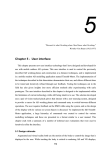
5.1.1. Video see-through
The simplest approach is the video see-through, as depicted in Figure 8. To get a sense of
immersion in virtual reality systems, head-mounted displays (HMD) that fully encompass the
user’s view are commonly employed. In this configuration, the user does not see the real
world directly, but instead only sees what the computer system displays on the tiny monitors
inside the HMD. The video camera continuously captures individual frames of the real world
and feeds each one into the augmentation system. Virtual objects are then merged into the
frame, and this final merged image is what users ultimately see in the HMD. By processing
each frame individually, the augmentation system can use vision-based approaches to extract
pose (position and orientation) information about the user for registration purposes (by
tracking features or patterns, for example). Since each frame from the camera must be
processed by the augmentation system, there is a potential delay from the time the image is
captured to when the user actually sees the final augmented image. Finally, the quality of the
imagery is limited by the resolution of the camera. The use of a stereo camera pair (two
cameras) allows the HMD to provide a different image to each eye, thereby increasing the
realism and immersion that the augmented world can provide. A large offset between the
cameras and the user’s eyes can further reduce the sense of immersion, since everything in the
captured scenes will be shifted higher or lower than where they should actually be (with
respect to the user’s actual eye level). The displays available at the time of writing has quite
narrow fields of view which will make them tiresome to use for longer periods of time.
Head-mounted
Display (HMD)
Video camera
Video of real world
Real
world
Users
view
Head
position
display
Graphics
system
Virtual
objects
Video
merging
Figure 8 Video see-through
9/70
Augmented video
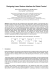
5.1.2. Optical see-through
The other popular HMD configuration for augmented reality is the optical see-through display
system, as depicted in Figure 11. In this setup, the user is able to view the real world through
a semi-transparent display, while virtual objects are merged into the scene optically in front of
the user’s eyes based on the user’s current position. Thus when users move their heads, the
virtual objects maintain their positions in the world as if they were actually part of the real
environment. Unlike the video see-through displays, these HMDs do not exhibit limited
resolutions and delays when depicting the real world. However, the quality of the virtual
objects will still be limited by the processing speed and graphical capabilities of the
augmentation system. Therefore, creating convincing augmentations becomes somewhat
difficult since the real world will appear naturally while the virtual objects will appear
pixelated. Another disadvantage with optical see-through displays is their lack of single frame
captures of the real world, since no camera is present in the default hardware setup. Thus
position sensors within the HMD are the only facility through which pose information can be
extracted for registration purposes. Some researchers have proposed hybrid solutions [54][84]
that combine position sensors with video cameras in order to improve the pose estimation.
Head position
Graphics
system
Head-mounted
Display (HMD)
Virtual objects
display
Users
view
Real
world
Optical
merging
Figure 9 Optical see through
5.1.3. Other solutions
Projection based displays. In this approach, the desired virtual information is projected
directly on the physical objects to be augmented. In the simplest case, the intention is for the
augmentations to be coplanar with the surface onto which they project and to project them
from a single room-mounted projector, with no need for special eyewear. Another approach
10/70
for projective AR relies on headworn projectors, whose images are projected along the
viewer’s line of sight at objects in the world. The target objects are coated with a
retroreflective material that reflects light back along the angle of incidence. Multiple users can
see different images on the same target projected by their own head-worn systems, since the
projected images can’t be seen except along the line of projection. By using relatively low
powered output projectors, nonretroreflective real objects can obscure virtual objects.
Projectors worn on the head can be heavy.
Monitor based. This is a technique known as monitor based or fishtank based AR and it is
the most avaliable solution for AR, where an ordinary personal computer and a web cam is all
you need. It works in the same way as video see through AR, with the only difference that the
users are not wearing the display and therefore do not get any immersive feeling. A subgroup
of these are the handheld devices where the user actually can get some kind of immersion.
The handheld device can act as a kind of magic magnifying glass showing virtual content
when moving the device over objects.
5.1.4. Other senses
Hearing. The sense of hearing helps us learn from each other through communication. Sound
can be used in augmented reality to enhance the experience of augmented reality and to
reduce or even remove sounds.
Touch. The sense of touch helps us learn about our world by feeling it and learning the size,
texture and shape of things. By introducing haptic feedback many applications for augmented
reality could be enhanced. Introducing touch is a difficult problem since the user has to have
some kind of physical object to provide the sensation. For example if a user would like to pick
up a virtual can standing on a real table the user could be wearing some kind of computercontrolled glove. Other augmentations like letting a user climb a virtual tree seem more or
less impossible to achieve.
Smell. The sense of smell helps us enjoy life and helps us learn about unsafe conditions. It
would be very difficult to augment smells as it would require some kind of device that can
artificially produce smells and blend them with the already present ones.
Taste. Taste helps us, among other things, to select and enjoy food. There are four tastes
(sweet, sour, salt and bitter). Similar to smell this would be extremely difficult to realize.
Fortunately smelling and tasting are the least dominant senses for humans and therefore
would make the smallest difference to augmented reality.
11/70
6. Mathematics of Augmented Reality
Before we can discuss the various solutions that have been proposed to solve the registration
problem (see chapter 7, [8]), we need to review some key mathematical ideas.
6.1. Coordinate Systems
The mathematical nature of the registration problem that has to be solved is depicted in
Figure 10. The three transformations that all augmented reality applications need to consider
are Object-to-world, World-to-camera, and Camera-to-image plane.
Camera
coordinates
( X c , Yc , Z c )
Camera screen
coordinates
( xs , ys )
World coordinates
( X w , Yw , Z w )
Figure 10 Augmented Reality Coordinate Systems
Object-to-world ( M O )
Assuming that we have a virtual object centered on its own local coordinate system, M O will
specify the transformation from this local system into a position and orientation within the
world coordinate system that defines the real scene.
World-to-camera ( M C )
The M C transformation specifies the position and orientation (pose) of the video camera that
is being used to view the real scene, allowing points in the real world to be specified in terms
of the camera’s origin.
Camera-to-image plane ( M P )
The M P transformation defines a projection from 3D to 2D such that camera coordinates can
be converted into image coordinates for final display onto a monitor or HMD. In order for an
augmented reality application to correctly render a virtual 3D object on top of a real scene, the
above three geometric transformations have to be accurate. An error in any one of the
relationships will cause the registration to be inaccurate, reducing the realism of the final
augmented scene.
Since the virtual 3D objects will be rendered using standard 3D graphics hardware, it follows
that they must be represented using traditional computer graphics data structures. The surface
12/70
of our virtual object can thus be represented as a triangular mesh, which consists of a set of
3D vertices and a set of non-overlapping triangles connecting these vertices. Using
homogeneous coordinates, the obvious approach to augmenting these virtual objects requires
that we determine the 2D projection [u, v, h] of a 3D point in Euclidean space [x, y, z, w]
using the following equation:
T
T
[u v h] = M P(3×4) M C ( 4×4) M O( 4×4) [ x y z w]
The following sections will discuss ideas from projective vision that allow us to explicitly
determine the M P , M C , and M O transformations.
6.2. Camera Models
Assuming we have a [x, y, z] vertex in camera coordinates, projective geometry allows us to
define the transformation M P that can convert this 3D point into 2D image space.
6.2.1. The Perspective Camera
Y
X
Focal length
Image
plane
Principal
point
Focal
point
Z
p
P
Figure 11 The pinhole camera
Figure 11 shows the perspective or pinhole camera model, which is considered the most
common geometric model for video cameras. The optical axis is defined as the line through
the center of focus (a 3D point), which is perpendicular to the image plane. The distance
between the image plane and the center of focus is referred to as the focal length (f). The
principal point is the intersection of the optical axis and the image plane. Assuming we have
any other point P = [X, Y, Z] in 3D, and if we consider the image plane to define our 2D
image, then the 2D projection of P is the intersection between the image plane and the line
through the center of focus and P, denoted by p = [x, y]. In other words, we have
X
x= f
Z
Y
y= f
Z
6.2.2. The Weak-Perspective Camera
Since the perspective projection is a non-linear mapping, it tends to make vision problems
difficult to solve. A commonly used approximation to the perspective camera model that
simplifies certain computations is the weak-perspective camera. If, for any two points in a
scene, the relative distance along the optical axis, δ Z , is significantly smaller than the average
13/70
depth, Z Avg , of the scene, then the approximation holds. Typically, δ Z < Z Avg 20 .
Conceptually, we can think of the projection as a two-step projection. The first is a projection
of the object points onto a plane that goes through Z Avg . The second is a uniform scaling of
the Z Avg plane onto the image plane. Mathematically, we have
x= f
X
Z Avg
(1)
Y
y= f
Z Avg
Typically, ZAvg can be the centroid of some small object in a scene.
ZAvg
Figure 12 Weak perspective camera
6.3. Camera Parameters
There are two subsets of camera parameters that can be used to determine the relationship
between coordinate systems. Known as the intrinsic and extrinsic parameters in the computer
vision field, they are defined as follows:
14/70
6.3.1. Intrinsic Camera Parameters
The intrinsic parameters are those related to the internal geometry of a physical camera. In
other words, they represent the optical, geometric, and digital characteristics of a camera. The
parameters are:
1. The focal length
2. The location of the image center in pixel space
3. The pixel size in the horizontal and vertical directions
4. The coefficient to account for radial distortion from the optics
The second and third parameters allow us to link image coordinates (xim, yim), in pixels, with
the respective coordinates (x, y) in the camera coordinate system. This is done quite simply:
x = − ( xim − ox ) sx
(2)
y = − ( yim − oy ) s y
where ( ox , oy ) define the pixel coordinates of the principal point, and ( sx , s y ) define the size
of the pixels (in millimeters), in the horizontal and vertical directions respectively. Using
Figure 11 as our reference, the sign change is required if we assume that the image has its x
coordinates increasing to the right, and the y coordinates increasing going down, with the
origin of the image in the top-left corner. The final parameter allows us to account for radial
distortions that are evident when using camera optics with large fields of view. Typically, the
distortions are most pronounced at the periphery of the image, and thus can be corrected using
a simple radial displacement of the form
x = xd 1 + k1r 2 + k2 r 4
(3)
y = yd 1 + k1r 2 + k2 r 4
(
(
where
)
)
( xd , yd )
is the distorted point in camera space, and r 2 = xd2 + yd2 , k1 and k2 are
additional intrinsic camera parameters, where k2 « k1. Usually k2 is set to 0. In many cases,
radial distortion can be ignored unless very high accuracy is required in all parts of the image.
6.3.2. Extrinsic Camera Parameters
The extrinsic parameters are concerned with external properties of a camera, such as position
and orientation information. They uniquely identify the transformation between the unknown
camera coordinate system and the known world coordinate system. The parameters, as
depicted in Figure 13, are:
1. The 3×3 rotation matrix R that brings the corresponding axes of the two coordinate
systems onto one another
2. The 3D translation vector T describing the relative positions of the origins of the two
coordinate systems
In other words, if we have a point Pw in world coordinates, then the same point in camera
coordinates, Pc, would be:
Pc = RPw + T
where
⎡ r00
R = ⎢⎢ r01
⎢⎣ r02
r10
r11
r12
(4)
r20 ⎤
r21 ⎥⎥
r22 ⎥⎦
(5)
15/70
defines the rotational information.
Therefore, if we ignore radial distortions, we can plug Eq.(2) and Eq.(4) into our perspective
projection equation, resulting in:
R1T ( Pw − T )
− ( xm − ox ) sx = f T
R3 ( Pw − T )
(6)
R2T ( Pw − T )
− ( ym − o y ) s y = f T
R3 ( Pw − T )
where Ri , i = 1, 2, 3, denotes the 3D vector formed by the i-th row of the matrix R.
Separating the intrinsic and extrinsic components, and placing the equations into matrix
form, we get:
⎡ f u 0 ox ⎤
(7)
M int = ⎢⎢ 0 f v o y ⎥⎥
⎢⎣ 0 0 1 ⎥⎦
where fu = -f / sx and
image space, and
⎡ r00 r10 r20
M ext = ⎢⎢ r01 r11 r21
⎢⎣ r02 r12 r22
fv = -f / sy, which defines the transformation between camera space and
t1 ⎤
t2 ⎥⎥
t3 ⎥⎦
(8)
where t1 = − R1T T , t2 = − R2T T and t3 = − R3T T , which defines the transformation between
world coordinates and camera coordinates.
Therefore, our projection equation can now be expressed in homogeneous matrix form:
⎡ xw ⎤
⎡ x1 ⎤
⎢ ⎥
⎢ x ⎥ = M M ⎢ yw ⎥
(9)
ext
int
⎢ 2⎥
⎢ zw ⎥
⎢⎣ x3 ⎥⎦
⎢ ⎥
⎣1⎦
where x1/x3 = xim and x2/x3 = yim.
Going back to our camera models, and setting some reasonable constraints on our parameters
(ox = 0, oy = 0), we can express the perspective projection matrix as simply:
M = M int M ext
Similarly, the weak-perspective camera matrix is:
⎡ f u r00 fu r01 f u r02
⎤
f u t0
⎢
⎥
M wp = M int M ext = ⎢ f v r10 fu r11 fu r12
f u t1
⎥
T
⎢⎣ 0
′
0
0
R3 ( P − T ) ⎥⎦
where P′ is the centroid of two points, P1 and P2 in 3D space.
6.4. Camera Calibration
Now that we have defined our camera models and camera parameters, we have a method to
associate the various coordinate systems from Figure 10. However, this assumes that we know
16/70
the actual values of our intrinsic and extrinsic parameters. The process of determining the
intrinsic and extrinsic camera parameters is known as the camera calibration problem.
The basic idea is to solve for the camera parameters based on the projection equations of
known 3D coordinates and their associated 2D projections. Six or more such correspondences
are required in order to solve a linear system of equations that can recover the twelve
elements of a 3×4 projection matrix. There are two common methods for camera calibration.
The first method attempts to directly estimate the intrinsic and extrinsic parameters based on
finding features in a known calibration pattern. The second method first attempts to estimate
the projection matrix linking world and image coordinates, and then uses the entries of this
matrix to solve for the camera parameters.
The major difficulty with these calibration approaches is the need to perform them manually
in a separate calibration procedure. For the purposes of augmented reality, efficient and
accurate camera calibration remains an open problem.
17/70
7. Registration
Although different usage areas of AR have different problems, the main issue is generally the
registration problem. The objects of the virtual and the real world must be perfectly aligned at
all times or the illusion of coexistence will fail. The same problems exist in virtual reality as
well, but due to the total immersion they are not as serious as in augmented reality. The
virtual reality is helped by the fact that the visual sense is the strongest of our senses and can
override the others in case of conflict. For example if we are in a totally immersed virtual
environment and turn our head 20 degrees and the eyes register 19 degrees the visual sense
will override the sense of balance and accept that we have actually turned 19 degrees. If this
error would happen in AR it would be visually apparent that we have turned 20 degrees and
therefore unacceptable. Research shows [39] that the human eye has a resolving power of a
small fraction of a degree. So in order to obtain perfect registration one needs to build a
system that has higher resolution than the human sensory system. Although this kind of
system is not likely to appear in the near future most applications are usable at much lower
resolutions due to the fact that the human brain automatically compensates for small errors in
order to understand what it perceives. If the visual errors are kept at a sub pixel level we will
actually never be able to detect them at all.
Tracking
AR requires technology that can accurately measure the position and orientation of a user in
the environment, referred to as tracking. Although tracking can be applied to the whole body
current research concentrates on tracking head movements. This section will try to overview
the basic principles of tracking position and orientation instead of individual systems.
For tracking to work effectively in Augmented Reality it should be accurate and at interactive
speed. This overview uses the six principles used in [55]: time of flight (TOF), spacial scan,
inertial sensing, mechanical linkages, phase-difference sensing and direct field sensing.
7.1. Time of flight
7.1.1. Ultrasonic
The time of flight principle relies on measuring the time of propagation of acoustic signals
between points, assuming that the propagation speed is constant. The most common
frequency used is in the ultrasonic range, typically around 40 kHz, to prevent the user from
hearing it. By using three emitters and three receivers, the position and orientation of the
target can be calculated using triangulation
Reference
Target
Figure 13 Ultrasonic tracker
18/70
Problem with such a system is that the speed of sound varies with pressure, humidity,
turbulence and it is sensitive to noise and line of sight. There is also a limit in the range of the
system due to the loss of energy with the distance travelled. The update rate of the system is
limited by the speed of sound. For this to work the reference will need to introduce a small
delay between its three emissions so that the target can distinguish them. This fact reduces the
maximum update rate by a factor three. Due to the sequential emissions this technique also
has an error that is proportional to the speed of the target. A general solution to the sequential
problem is to send emissions simultaneously using different frequencies.
7.1.2. Electromagnetic
By using electromagnetic signals instead of ultrasonic the update rate of the system can be
increased dramatically but errors in time measures result in large position errors due to the
speed of light. Such a system is the global positioning system (GPS) that uses 24 satellites and
12 ground stations spread around the world. Each satellite has an atomic clock that is
recalibrated every 30 sec. The resolution accomplished with such a system is on the order of
10 meters. A more precise system, the differential GPS, uses emitting ground stations that
refine the resolution to the order of a meter [46]. Drawbacks of GPS systems are their poor
accuracy and resolution, and the failure of the technology if the direct lines of sight to the
satellites are occluded.
7.1.3. Optical gyroscopes
Gyroscopes measure angular velocity. Optical gyroscopes rely on interferometry, i.e. optical
interference. A laser beam is divided in two waves that travel within the interferometer in
opposite directions. For no rotation, both waves combine out of phase because of the
consecutive π phase shifts at mirror reflection. For a clockwise rotation of the device, the
wave front propagating counter-clockwise travels a shorter path than the wave front
propagating clockwise, producing interference at the output. The number of fringes is
proportional to the angular velocity. Note: Although the phenomenon comes from TOF the
measured variable is not time.
7.2. Inertial sensing
The principle is based on the attempt to preserve either a given axis of rotation (gyroscope) or
a position (accelerometer)
7.2.1. Mechanical gyroscope
A mechanical gyroscope, in its simplest form, is a system based on the principle of
conservation of the angular momentum that states that an object rotated at high angular speed,
in the absence of external moments, conserves its angular momentum. A gyroscope makes a
two degrees of freedom orientation tracker, thus at least two gyroscopes with perpendicular
axes are needed to make a full 3DOF orientation tracker. The problem with mechanical
gyroscopes is that the friction causes a small drift but periodic recalibrations (usually about
once a second) will increase accuracy.
7.2.2. Accelerometer
An accelerometer measures the linear or angular acceleration of an object to which it is
attached. It is a one degree of freedom device that generally consists of a small mass and a
spring supporting system. Single and double integration of the output gives the speed and
position. The unknown constants introduced in the integration cause an error. Accelerometers
are small and cheap. Accelerometers in general drift a lot and need to be recalibrated several
times a second. Due to this they are most often used in combination with other tracking
techniques for tracking swift movements.
19/70
7.3. Mechanical linkages
This type of tracking system uses mechanical linkages between the reference and the target.
Two types of linkages have been used. One is an assembly of mechanical parts that can each
rotate providing the user with multiple rotation capabilities. The orientations of the linkages
are computed from the various linkages angles measured with incremental encoders or
potentiometers. Other types of mechanical linkages are wires that are rolled on coils. A spring
system ensures that the wires are tensed in order to measure the distance accurately. The
degrees of freedom sensed by mechanical linkage trackers are dependent upon the
constitution of the tracker mechanical structure. While six degrees of freedom are most often
provided, typically only a limited range of motions is possible because of the kinematics of
the joints and the length of each link. Also, the weight and the deformation of the structure
increase with the distance of the target from the reference and impose a limit on the working
volume. Mechanical linkage trackers have found successful implementations among others in
force-feedback systems used to make the virtual experience more interactive.
7.4. Phase difference
Phase-difference systems measure the relative phase of an incoming signal from a target and a
comparison signal of the same frequency located on the reference. As in the TOF approach,
the system is equipped with three emitters on the target and three receivers on the reference.
Ivan Sutherland’s head tracking system, built at the dawn of time when it comes to virtual
reality, explored the use of an ultrasonic phase-difference head tracking system and reported
preliminary results [68]. In Sutherland’s system, each emitter sent a continuous sound wave at
a specific frequency. All the receivers detected the signal simultaneously. For each receiver,
the signal phase was compared to that of the reference signal. A displacement of the target
from one measurement to another produced a modification of the phases that indicated the
relative motion of the emitters with respect to the receivers. After three emitters had been
localized, the orientation and position of the target could be calculated. It is important to note
that the maximum motion possible between two measurements is limited by the wavelength
of the signal. Current systems use solely ultrasonic waves that typically limit the relative
range of motion between two measurements to 8 mm. Future systems may include phasedifference measurements of optical waves as a natural extension of the principle that may find
best application in hybrid systems. Because it is not possible to measure the phase of light
waves directly, interferometric techniques can be employed to this end. The relative range of
motion between two measurements will be limited to be less than the wavelength of light
unless the ambiguity is eliminated using hybrid technology.
7.5. Direct field sensing
7.5.1. Magnetic field sensing
By circulating an electric current in a coil a magnetic field is generated. By placing a
magnetic receiver in the vicinity a flux is introduced in the receiver. The flux is a function of
the distance and the orientation of the receiver relative to the coil. The emitted field could
either be an artificial one, making it possible to do six degrees of freedom measurements
relative to the reference or the natural magnetic field of the earth making it a one degree of
freedom tracker relative to the earth (compass). Magnetic trackers are inexpensive,
lightweight, compact and do not suffer from occlusion. They are limited in range by the
strength of the emitted electromagnetic field and are sensitive to metallic objects and
electromagnetic noise. Using multiple emitters can expand the range.
20/70
7.5.2. Gravitational Field Sensing
An inclinometer operates on the principle of a bubble clinometer. Common implementations
use electrolytic or capacitive sensing of fluids. A simple implementation may measure the
relative level of fluids in two branches of a tube to compute inclination. A common
implementation measures the capacitance of a component being changed based on the level of
fluid in the capacitor. Inclinometers are inexpensive, reference-free one degree of freedom
orientation trackers that are limited in update rate by the viscosity of the fluid used.
Figure 14 Bubble clinometer
7.6. Spacial scan
7.6.1. Beam scanning
This technique uses scanning optical beams on a reference. Sensors on the target detect the
time of sweep of the beams on their surface. This technique has very limited working volume
and is only used in a small number of applications, for example tracking a pilot’s head
orientation in airplane cockpits.
7.7. Vision based
Vision based pattern recognition
Vision based trackers rely on light propagated along a line of sight to determine the position
of a target in 3D space. Generally there are three types of sensors used for vision-based
tracking [12]:
• CCD sensors
• CMOS sensors
• LinLog sensors
Charge Coupled Device (CCD) sensors have an array of capacitors whose charges are
determined by the light intensity. CCDs are normally used in video cameras and are very
popular in video-see-through AR.
CMOS sensors are an integration of analog sensor circuitry and digital image processing onto
a single chip. CMOS offers much higher sensitivity than CCD and has an internal structure
similar to random access memory blocks making it easy to access parts of the captured image.
A CMOS sensor can track sub images at several kfps.
LinLog sensors have the ability to separate the mapping between incident illumination and
pixel response in a linear and a logarithmic part. This means that they can adjust the range of
linear operation without any further computations, which is useful in extreme illumination
conditions.
21/70
The input of a visual tracker is a sequence of 2D images taken from a 3D scene. As the
amount of information in each image is very large only parts of the image are used for
tracking. These parts are selected based on knowledge of the object to track and are
commonly known as feature based tracking. Since the acquired images are used not only for
tracking, but also for a presentation of the scene, the most popular image acquisition device is
a CCD based video camera mounted on a user’s head.
This is the general pipeline of a video see-through system that uses the acquired image for
both tracking and presentation:
Image capture
Pattern recognition
Coordinate calculation Image rendering Image display
Figure 15 Image pipeline of video see-through tracker
The key issue in real-time tracking is to robustly detect features in the input images within a
short period of time. In order to achieve this goal artificial features can be put in the scene that
have good properties for tracking. These are usually high contrast patterns known as fiducials.
7.7.1. Fiducial based
Determining the position and orientation of the camera is an important problem. Ideally we
would like to obtain this information without prior knowledge about the cameras
environment. In this regard stereovision is a natural choice, however stereo is computationally
expensive.
7.7.1.1. Determining the distance and orientation of a quadrangle
If prior knowledge of the environment is available then we can proceed differently. For
example it is known that the orientation of a planar surface can be recovered by computing
the perspective projection vanishing points of groups of parallel lines on the planar surface.
Let Pi , i = 0,...,3 , be the position vectors of the vertices of a planar quadrangle, denoted by
< P0 , P1 , P2 , P3 > , in a given coordinate system. Then there exists a pair of real numbers, α ,
β , such that P3 = P0 + α ( P1 − P0 ) + β ( P2 − P0 ) . Note that the values of α and β are
independent of the choice of the coordinate system, and that noncolinearity implies that
α + β ≠ 1 . Obviously neither α nor β is zero.
22/70
y
Image plane
x
P0
Focal center
v2
P2
w0
v0
w2
v1
z
w1
P1
v3 = w3
(0,0,f)
P3
Figure 16 Quadrangle
Let Vi , i = 0,...,3 be the position vectors of the perspective projections of Pi on the image
plane (see Figure 16). Then Vi determines the ray on which Pi must lie – i.e., there exist
ki > 0 such that Pi = kiVi . Two questions arise:
1. Is K = {ki | i = 0,...,3} a unique set?
2. How do we determine it?
K is indeed unique and can easily be determined from the Vi s and Pi s.
Theorem [32]:
Given a pyramid, there cannot exist two different planes cutting the pyramid in identical
quadrangles – i.e., if { P0 , P1 , P2 , P3 } and {Q0 , Q1 , Q2 , Q3 } are the vertices of any two
quadrangles with Pi , Qi on the i-th edge of the pyramid, and if the two quadrangles are
identical, then Pi = Qi for all i = 1,..,3 .
Proof:
Without loss of generality, assume that the peak of the pyramid is at the origin.
Since Pi , Qi are on the same edge, there exists ki > 0 such that Qi = ki Pi , i = 0,...,3 .
Since the Pi s are coplanar, we know that there exist α , β , neither of them equal to zero,
and α + β ≠ 1 , such that P3 = P0 + α ( P1 − P0 ) + β ( P2 − P0 ) . This relation also holds for
Q0 , Q1 ,Q2 ,Q3
i.e. there exists another pair of numbers
Q3 = Q0 + α ′ ( Q1 − Q0 ) + β ′ ( Q2 − Q0 ) .
23/70
α ′, β ′
such that
Assuming that these two quadrangles are identical, then α ′ = α and β ′ = β .
Substituting Qi = ki Pi gives
k
k
k
k3 P3 = k0 P0 + α ( k1 P1 − k0 P0 ) + β ( k2 P2 − k0 P0 ) ⇒ P3 = 0 (1 − α − β ) P0 + 1 α P1 + 2 β P2
k3
k3
k3
But P0 , P1 , P2 are linearly independent, and we already know that
P3 = (1 − α − β ) P0 + α P1 + β P2
Thus we conclude that
k0 k1 k2
= = = 1 , and then
k3 k3 k3
Q0 − Q1 i = P0 − P1 i ⇔ k0 P0 − P1 i = P0 − P1 i ⇒ ki = 1 for all i = 0,...,3
Assume that we have the image plane as shown in Figure 16, and that we know the focal
length. Also assume that we know the dimensions of the known quadrangle – that is, we know
the distance between each of the six pairs of the four vertices, and the values of α and β as
defined above.
Let Pi , i = 0,...,3 , be the position vectors of the vertices of the quadrangle in the camera
frame, and let Vi , i = 0,...,3 , be the position vectors of the corresponding image points. Then,
obviously there exist ki > 0, i = 0,...,3 , such that Pi = kiVi . Following the argument in the
above theorem, we have
k0
k
k
(10)
(1 − α − β )V0 + 1 αV1 + 2 β V2 = V3
k3
k3
k3
Since V0 , V1 , V2 ,V3 are linearly independent, ⎡⎣(1 − α − β ) V0 ,αV1 , β V2 ⎤⎦ , which is a 3×3 matrix,
k k
k
is invertible. So we can solve for 0 , 1 , and 2 . What remains is to determine k3 . Since
k3
k3 k3
k
< 0 (1 − α − β )V0 , αV1 , β V2 , V3 > , shown as < W0 , W1 ,W2 ,W3 > in Figure 16, is a quadrangle
k3
obtained by shrinking the original quadrangle < P0 , P1 , P2 , P3 > along the edges of the pyramid
until V3 is reached, it is similar to < P0 , P1 , P2 , P3 > . Therefore k3 can be determined by the
relationship
P0 − P3 2
k3 =
k0
(1 − α − β )V0 − V3
k3
2
Following the above procedure, we can recover the 3D positions of Pi , i = 0,...,3 in the
camera frame.
The technique directly solves for the absolute positions of the vertices of the given
quadrangle in the camera-centered frame (obviously the orientation of the quadrangle and the
distance to, say, its center can be easily computed from Pi ). Its implementation only requires
knowledge of the relation among four coplanar points and their corresponding image
coordinates. The computational effort only involves solving a system of three linear equations
in three unknowns and some simple arithmetic operations.
24/70
7.7.1.2. Determining the elements of exterior orientation of the camera
The elements of exterior orientation of a camera express its position and angular orientation
(or pose) in the fixed world frame. The pose is expressed in terms of three consecutive
rotations with angles (θ , φ ,ψ ) . These rotations define the angular relationships between the
three axes of the world coordinate system.
7.7.1.3. Decomposing the rotation component
The problem of determining the elements of exterior orientation can be solved with the
results from the previous section. Let Pi , i = 0,...,3 be the world coordinates of four coplanar
points. Then, by applying the method from above, we can determine their corresponding
coordinates in the camera coordinate system. We call them Qi , i = 0,...,3 . From this
correspondence we can determine the transformation from the world frame to the camera
frame. Decomposing this transformation matrix, Λ , into its translation, T, and rotation, R,
components, we will have recovered the six elements of exterior orientation.
R, as described above, is the result of three consecutive rotations, i.e. R = Rψ Rφ Rθ , where
⎡cosθ 0 − sin θ ⎤
Rθ = ⎢⎢ 0
1
0 ⎥⎥ is the rotation around the Y-axis,
⎢⎣ sin θ 0 cos θ ⎥⎦
0
0 ⎤
⎡1
⎢
Rφ = ⎢0 cos φ sin φ ⎥⎥ is the rotation around the X-axis,
⎢⎣0 − sin φ cos φ ⎥⎦
⎡ cosψ sin ψ 0 ⎤
Rψ = ⎢⎢ − sin ψ cosψ 0 ⎥⎥ is the rotation around the Z-axis.
⎢⎣ 0
1 ⎥⎦
0
It follows that:
⎡cosθ cosψ + sin θ sin φ sin ψ cos φ sin ψ − sin θ cosψ + cos θ cos φ sinψ ⎤
R = ⎢⎢cosθ sinψ + sin θ sin φ cosψ cos φ cosψ sin θ sin ψ + cos θ sin φ cosψ ⎥⎥
⎢⎣
⎥⎦
sin θ cos φ
sin φ
cos θ cos φ
also noted as:
⎡ r00 r10 r20 ⎤
R = ⎢⎢ r01 r11 r21 ⎥⎥
⎢⎣ r02 r12 r22 ⎥⎦
From r21 = − sin φ we get two possible solutions for φ which are
⎧φ+ = arcsin ( − r21 )
⎨
⎩ φ− = π − φ+
If cos φ ≠ 0 then we can solve for the corresponding ψ from
⎧ r01 = cos φ sin ψ
⎨
⎩r11 = cos φ cosψ
and solve for θ from
⎧r00 = cosθ cosψ + sin θ sin φ sin ψ
⎨
⎩ r10 = cos θ sin ψ + sin θ sin φ cosψ
25/70
Let ψ + , θ + be the solutions obtained by choosing φ = φ+ , and let ψ − , θ − be similarly defined.
Then it is easy to see that
⎧ψ − = π + ψ +
⎨
⎩ θ− = π + θ+
This implies that
r02 = sin θ + cosψ + + cosθ + sin φ+ sinψ +
= sin θ − cosψ − + cos θ − sin φ− sin ψ −
r12 = − sin θ + sinψ + + cos θ + sin φ+ cosψ +
= − sin θ − sin ψ − + cosθ − sin φ− cosψ −
r22 = cos θ + cos φ+
= cosθ − cos φ−
In other words, the two sequences of rotations Rψ + Rφ+ Rθ + and Rψ − Rφ− Rθ − are equivalent. Thus
either of the triples (θ + , φ+ ,ψ + ) and (θ − , φ− ,ψ − ) can be chosen as the pose of the camera. We
⎡ π π⎤
choose the one with positive subscripts. Note that φ+ ∈ ⎢ − , ⎥ .
⎣ 2 2⎦
If cos φ = 0 , we have two possibilities.
⎡cos ω1
π
1) φ = − : letting ω1 = θ −ψ , R can be expressed as R = ⎢⎢ sin ω1
2
⎣⎢ 0
− sin ω1 ⎤
0 cos ω1 ⎥⎥
0 ⎦⎥
−1
0
Then it is easy to solve for ω1 = θ − ψ , which gives us ψ = θ − ω1 .
⎡cos ω 2 0 − sin ω 2 ⎤
2) φ = − : letting ω 2 = θ + ψ ,R can be expressed as R = ⎢⎢ sin ω 2 0 cos ω 2 ⎥⎥
2
⎢⎣ 0
0 ⎥⎦
−1
Again we can solve for ω 2 = θ + ψ , which gives us ψ = ω 2 − θ . Thus if cos φ = 0 , we have an
infinite number of equivalent solutions of the form
π
φ=
π
2
,ψ = θ − ω1 ,θ ∈ [ 0, 2π ] , or
π
φ = − ,ψ = ω 2 − θ ,θ ∈ [ 0, 2π ] .
2
Since in each case all the solutions are equivalent, we can stipulate that θ = 0 , and designate
the pose as
θ = 0, φ =
π
2
,ψ = −ω1 , or
π
θ = 0, φ = − ,ψ = ω 2
2
It is worth noting that in the above derivation, we only need the first two columns of the
rotation matrix R.
26/70
7.7.1.4. Determining the position of the origin of the camera frame
Now, let V0 be the position of the origin of the camera coordinate system in the world frame,
and T4 be the first three elements of the fourth column of the transformation matrix Λ . Then
since
T4 = Rψ Rφ Rθ ( −V0 ) Æ V0 = − Rθ−1 Rφ−1 Rψ−1T4
we can recover the position of the origin of the camera coordinate system in the world frame.
The problem is to find the transformation matrix Λ .
7.7.1.5. Determining the transformation matrix
First assume that the vertices of the quadrangle are situated in such a manner that their
coordinates in the world frame (XYZ) have simple forms (see Figure 16 Quadrangle).
P0 = ( 0, 0, 0,1) , P1 = ( X 1 , 0, 0,1) , P2 = ( X 2 , Y 2 , 0,1) , P3 = ( X 3 , Y3 , 0,1)
T
T
T
T
Let Qi = ( xi , yi , zi ,1) , i = 0,...,3 be their corresponding coordinates in the camera frame
T
(xyz); then we have
Qi = ΛPi , or Q = ΛP
where
Q = ( Q0 , Q1 , Q2 , Q3 ) , and P = ( P0 , P1 , P2 , P3 )
(11)
are 4×4 matrices. The fourth column of Λ , which is the translation component, can be readily
seen to be ( x0 , y0 , z0 ,1) . Since the matrix P is of a simple form, we can solve for the first two
columns of Λ easily. These are what is needed for the derivation of the three rotation angles
θ , φ and ψ .
If the four vertices are not situated in the manner described, then we can still find a
reference frame X ′ Y ′ Z ′ such that the coordinates of the four vertices in this frame,
Pi′ , i = 0,...,3 , have the form given above. The transformation, Λ1 from the XYZ frame to the
X ′ Y ′ Z ′ frame can be easily obtained, and we already know how to compute the second
transformation, Λ 2 , from the X ′ Y ′ Z ′ to the xyz frame, so the transformation, Λ , from the
XYZ frame to the xyz frame is given by Λ = Λ 2 Λ1 . Then the procedure developed earlier can
be used to compute the six elements of exterior orientation of the camera.
27/70
P3 = ( x3 , y3 , 0,1)
P1 = ( x1 , 0, 0,1)
P2 = ( x2 , y2 , 0,1)
P0 = ( 0, 0, 0,1)
Figure 17 Quadrangle in xy-plane
7.7.1.6. Shape restoration
The method described above is an exact algorithm, and as such is sensitive to noise. Here is
described a method which attempts to restore the shape of the quadrangle. The transformation
matrices from the marker coordinates to the camera coordinates ( Tcm ) represented in
Eq. (12) are estimated using the method described above:
⎡ X c ⎤ ⎡ R00 R10 R20 Tx ⎤ ⎡ X m ⎤
⎢ Y ⎥ ⎢R
⎥⎢ ⎥
⎢ c ⎥ = ⎢ 01 R11 R21 Ty ⎥ ⎢Y m ⎥ Æ
⎢ Z c ⎥ ⎢ R02 R12 R22 Tz ⎥ ⎢ Z m ⎥
⎢ ⎥ ⎢
⎥⎢ ⎥
0
0
1 ⎦⎣ 1 ⎦
⎣1⎦ ⎣ 0
⎡
⎢0
⎣
⎡Xm ⎤
⎡Xm ⎤
⎢
⎥
⎢Y ⎥
R 3×3
T3×1 ⎤ ⎢ Ym ⎥
= Tcm ⎢ m ⎥
⎢ Zm ⎥
0 0 1 ⎥⎦ ⎢ Z m ⎥
⎢ ⎥
⎢ ⎥
⎣ 1 ⎦
⎣ 1 ⎦
(12)
28/70
Camera
coordinates
( X c , Yc , Zc )
Camera screen
coordinates
( xc , yc )
Marker coordinates
( X m , Ym , Z m )
Figure 18 The relationship between marker and camera coordinates
All variables in the transformation matrix are determined by substituting screen coordinates
and marker coordinates of the detected marker's four vertices for ( xc , yc ) and ( X m , Ym )
respectively. After that, the normalization process can be done by using this transformation
matrix.
⎡ hxc ⎤ ⎡ N 00 N10 N 20 ⎤ ⎡ X m ⎤
⎢ hy ⎥ = ⎢ N
⎥⎢ ⎥
(13)
⎢ c ⎥ ⎢ 01 N11 N 21 ⎥ ⎢ Ym ⎥
⎢⎣ h ⎥⎦ ⎢⎣ N 02 N12
1 ⎥⎦ ⎢⎣ 1 ⎥⎦
When two parallel sides of a square marker are projected on the image, the equations of those
line segments in the camera screen coordinates are the following:
(14)
a1 x + b1 y + c1 = 0,
a2 x + b2 y + c2 = 0
For each of the markers, the value of these parameters has been already obtained in the linefitting process. Given the perspective projection matrix P that is obtained by the camera
calibration in eq.(11), equations of the planes that include these two sides respectively can be
represented as eq.(13) in the camera coordinates frame by substituting xc and yc in eq.(13)
for x and y in eq.(14).
⎡ Xc ⎤
⎡ P00 P01 P02 0 ⎤
⎡ hxc ⎤
⎢ ⎥
⎢ 0 P P 0⎥
⎢ hy ⎥
11
12
⎥,
⎢ c ⎥ = P ⎢ Yc ⎥
(15)
P=⎢
⎢ Zc ⎥
⎢0
⎢ h ⎥
0
1 0⎥
⎢ ⎥
⎢
⎥
⎢ ⎥
0
0 1⎦
⎣1⎦
⎣0
⎣ 1 ⎦
29/70
a1 P00 X c + ( a1 P01 + b1 P11 ) Yc + ( a1 P02 + b1 P12 + c1 ) Z c = 0
a2 P00 X c + ( a2 P01 + b2 P11 ) Yc + ( a2 P02 + b2 P12 + c2 ) Z c = 0
(16)
Given that the normal vectors of these planes are n1 and n2 respectively, the direction vector
of two parallel sides of the square is given by the outer product n1 × n2 . Given that two unit
direction vectors that are obtained from two sets of two parallel sides of the square are u1 and
u2 , these vectors should be perpendicular. However, image-processing errors mean that the
vectors will not be exactly perpendicular. To compensate for this two perpendicular unit
direction vectors are defined by v1 and v2 in the plane that includes u1 and u2 as shown in
Figure 19.
v1
u1
u2
v2
Figure 19
Given that the unit direction vector that is perpendicular to both v1 and v2 is v3 , the rotation
component V3×3 in the transformation matrix Tcm from marker coordinates to camera
coordinates specified in eq.(12) is ⎡⎣V0tV1tV2t ⎤⎦ .
Since the rotation component V3×3 in the transformation matrix was given, by using eq.(12)
and eq.(15), the coordinates of the four vertices of the marker in the marker coordinate frame
and those coordinates in the camera screen coordinate frame, eight equations including the
translation component WxWyWz are generated and the values of these translation components
WxWyWz can be obtained from these equations.
The transformation matrix found from the method mentioned above may include error.
However this can be reduced through the following process:
The vertex coordinates of the markers in the marker coordinate frame can be transformed to
coordinates in the camera screen coordinate frame by using the transformation matrix
obtained. Then the transformation matrix is optimized as a sum of the difference between
these transformed coordinates and the coordinates measured from the image goes to a
minimum. Though there are six independent variables in the transformation matrix, only the
rotation components are optimized and then the translation components are reestimated by
using the method mentioned above. By iteration of this process a number of times the
transformation matrix is more accurately found. It would be possible to deal with all of six
30/70
independent variables in the optimization process. However, computational cost has to be
considered.
7.7.2. Homographies
For pattern-based augmented reality, a planar pattern defines a world coordinate system into
which virtual objects will be placed. It would be convenient if the planar pattern itself could
be used to determine a projection matrix that could be directly applied to the coordinates of a
virtual object for augmentation purposes. This would eliminate the need for a separate
complicated calibration procedure, thus simplifying the system for the end-user. One way to
do this is to use a projective transformation technique called homography. Homography
comes from the observation that under perspective projection, the transformation between a
world plane and its corresponding image plane is projective linear. A homography is a one-toone mapping between two images, which is defined by only eight parameters. This model
exactly describes the image motion between two frames of a video sequence when
1. Camera viewing is pure rotation
2. Camera is viewing a planar scene
Usually, feature displacement between two images depends on both the camera movement
and the camera’s distance from the feature. A simple parameterized mapping is therefore not
possible. However, in many circumstances, the homography represents a good approximation
of the true image flow, particularly when the image structure is near planar, or the camera
movement is small and the scene structure is mostly distant.
Figure 20 Homography
Consider a set of points in the first image of a sequence with homogeneous coordinates
( xi , yi , zi ) , which are known to map to a set of points in the second image ( xi′, yi′, zi′ ) . The
relationship between the two images is a homography if the following equation holds:
31/70
⎡ xi′ ⎤ ⎡ h00 h10 h20 ⎤ ⎡ xi ⎤
⎡ xi ⎤
⎢ y′ ⎥ = ⎢ h
⎥⎢ ⎥
⎢ ⎥
⎢ i ⎥ ⎢ 01 h11 h21 ⎥ ⎢ yi ⎥ = H ⎢ yi ⎥
⎢⎣ zi′ ⎥⎦ ⎢⎣ h02 h12 h22 ⎥⎦ ⎢⎣ zi ⎥⎦
⎢⎣ zi ⎥⎦
In other words, the homography, H, maps coordinate x to coordinate x′. Note that these are
homogenous coordinates and that each point on the screen is treated as a ray through the
camera center. We find the actual image position by dividing the first and second components
by the third. The homography is therefore a simple linear transformation of the rays passing
through the camera center. Roughly speaking, the homography can encompass rotations,
scaling, and shearing of the ray bundle. We can rewrite the equation as
h x + h01 y + h02
x′ = 00
h20 x + h21 y + h22
h10 x + h11 y + h12
h20 x + h21 y + h22
where hij defines the [i, j ] -th element of H. This can be further rewritten as two linear
y′ =
equations
x′ ( h20 x + h21 y + h22 ) = h00 x + h01 y + h02
y′ ( h20 x + h21 y + h22 ) = h10 x + h11 y + h12
In matrix form we have
⎛ x y 1 0 0 0 − x′x − x′y − x′ ⎞
⎜
⎟h = 0
⎝ 0 0 0 x y 1 − y′x − y′y − y′ ⎠
where h = [ h00
h01
h02
h10
h11
h12
h20
h21
h22 ] is a 9-element vector containing the
T
elements of H. Therefore with four such non-colinear point correspondences, we can solve for
all the elements of H as follows
⎛ x0 y0 1 0 0 0 − x0′ x0 − x0′ y0 − x0′ ⎞
⎜
′
′
′⎟
⎜ 0 0 0 x0 y0 1 − y0 x0 − y0 y0 − y0 ⎟
⎜ x1 y1 0 0 0 0 − x1′x1 − x1′ y1 − x1′ ⎟
⎟
⎜
⎜ 0 0 0 x1 y1 1 − y0′ x0 − y0′ y0 − y0′ ⎟ h = Ah = 0
⎜ x y2 0 0 0 0 − x2′ x2 − x2′ y2 − x2′ ⎟
⎜ 2
⎟
⎜ 0 0 0 x2 y2 1 − y0′ x0 − y0′ y0 − y0′ ⎟
⎜ x y 0 0 0 0 − x′ x − x′ y − x′ ⎟
3
3 3
3 3
3
⎜ 3
⎟
⎜ 0 0 0 x y 1 − y′ x − y′ y − y′ ⎟
3
3
0 0
0 0
0⎠
⎝
The solution h is thus the null-space of the 8×9 matrix A, which can be solved using known
methods such as singular value decomposition Unfortunately, H alone cannot be directly used
to augment virtual 3D objects into the image, since the Z component from pattern space is
assumed to always be zero. However, recent works [58][86] show that if we know the camera
calibration matrix and have prior knowledge of the relative position of some points in the
plane we can calculate the camera’s full 3D transformation relative to the planar surface in the
same way as for fiducial tracking.
32/70
7.7.3. Optical Flow
Consider a point P that is depicted by a moving pinhole camera. Between two consecutive
frames, the camera has rotated ( Ω x , Ω y , Ω z ) around, and translated (Tx , Ty , Tz ) along its three
coordinate axes. This is equivalent to keeping the camera still and moving the point, which is
X
P2
P1
Tx
Tz
Ωx
p2
Z
Ωz
d
p1
Ty
Ωy
Y
Figure 21 The point p moves from p1 to p2 in the camera coordinate system due to rotational and
translational motion of the camera.
shown in Figure 21, where the point moves from P1 = ( X 1 , Y1 , Z1 ) to P2 = ( X 2 , Y2 , Z 2 ) . The
images in are denoted I ( x, y, t1 ) and I ( x, y, t2 ) (or I1 and I 2 for short), and the coordinates of
the points in the image plane are represented by p1 = ( x1 , y1 ) and p1 = ( x2 , y2 ) . The
displacement vector (α , β ) (denoted d in Figure 21) of the point ( x1 , y1 ) can be defined as
α = x2 − x1
β = y2 − y1
(17)
The displacement vector (α , β ) thus tells where to find a corresponding point from image I1
in image I 2 . If the displacement is defined for each pixel position ( x, y ) in image I1 , the
result is a displacement field, (α ( x, y ) , β ( x, y ) ) , where both α and β depend on x and y. A
pixel ( x1 , y1 ) in image I1 can then be found in ( x1 + α ( x1 , y1 ) , y1 + β ( x1 , y1 ) ) in image I 2
33/70
Closely related to the displacement field is the velocity field ( u, v ) , which is defined as the
velocity of a pixel in the image plane. Thus
dx
u=
dt
(18)
dy
v=
dt
where ( dx, dy ) is the displacement vector generated by camera motion during dt . In the same
manner as the displacement field, u and v are both functions of x and y; u = u ( x, y ) ,
v = v ( x, y ) . If the time Δt = t2 − t1 between the two frames I1 and I 2 is known, the velocities
u and v can be approximated using
x −x
α
u≈ 2 1 =
Δt
Δt
(19)
y2 − y1 β
v≈
=
Δt
Δt
Choosing the time scale such that Δt = 1 yields ( u, v ) ≈ (α , β ) . This blurs the border between
the velocity field and the displacement field.
If the object is fixed and only the camera moves, (or equivalently, if the camera is fixed but
the object moves rigidly), the motion can be described by a rigid body transformation,
P2 = RP1 + T
(20)
where R is a 3 × 3 rotation matrix and T = (Tx , Ty , Tz ) is a translation vector. Furthermore, the
projection from a three dimensional point to the image can be calculated using
X
x= f
Z
(21)
Y
y= f
Z
where f is the distance from the image plane to the center of projection as shown in Figure 21.
By assuming that f = 1 , that the rotation between frames is small, and that Tz Z = 1 , it is
shown [4] that the displacement field can be calculated using
u ( x, y ) ≈ −Ω x xy + Ω y (1 + x 2 ) − Ω z y + (Tx − Tz x ) Z
(22)
v ( x, y ) ≈ −Ω (1 + y 2 ) + Ω y xy + Ω z x + (Ty − Tz y ) Z
x
where Ω x , Ω y and Ω z are differential Euler angles around the x-, y- and z-axes respectively,
as shown in Figure 21.
34/70
Equation (22) is also valid for the velocity field. Setting ΔU = ( Ω x , Ω y , Ω z , Tx , Ty , Tz ) ,
equation (22) can be written in matrix notation
⎡u ⎤ ⎡ c u ⎤
⎢ v ⎥ = ⎢ u ⎥ ΔU
⎣ ⎦ ⎣v ⎦
or
⎡u ⎤
⎢ v ⎥ = C ΔU
⎣ ⎦
where
2
xy
x
0 1Z
⎡c u ⎤ ⎡ − (1 + y )
C = ⎢ v⎥ = ⎢
⎣ c ⎦ ⎢⎣ − xy
(1 + x2 ) − y 1 Z 0
(23)
(24)
− y Z⎤
⎥
− x Z ⎥⎦
(25)
7.7.4. The optical flow constraint
To estimate the optical flow, a model is needed that explains how the optical flow relates to
the image intensity. A common approach is to assume that the projection of an object point
onto a pixel preserves its brightness from one frame to another. This is not generally true,
since many materials reflect different amounts of light at different angles, but it is a
reasonable approximation. The assumption can be formulated
I ( x + u , y + v, t + 1) = I ( x, y, t )
(26)
Taylor expanding the left side of equation (26) around (x,y,t) and removing higher order terms
results in
I ( x, y , t ) + I x u + I y v + I t = I ( x , y , t )
(27)
I xu + I y v + I t = 0
The above equation is called the optical flow constraint equation, and is valid for small
movements between frames. The notation can be further simplified to
⎡u ⎤
⎡⎣ I x I y ⎤⎦ ⎢ ⎥ = − I t
(28)
⎣v ⎦
⎡u ⎤
∇I ⎢ ⎥ = − I t
(29)
⎣v ⎦
7.7.5. Solutions using fiducial tracking
Tracking artificial patterns with well-known properties is the most common way to do video
based tracking. Once recognized the coordinates of the pattern relative to the camera can be
calculated. Knowing the 2D location of 4 coplanar points gives one unique solution of the
coordinate system of the marker. To identify a marker a symbol of some kind is often used.
The symbol is matched with the reference using mean square error or standard deviation. The
markers can vary in size to improve tracking range. Most vision based tracking systems use
single size fiducials. This provides a small detection range due to the low resolution of current
CCD cameras. Youngkwan Cho et al [85] have developed a fiducial system that can be
detected at various ranges seamlessly. The idea is to use multi color multi size concentric
rings, where parts of the rings can be detected as fiducials themselves. They have also
developed a fiducial detection method that is less sensitive to varying lighting conditions
35/70
using light-invariant relationships between homogenous regions instead of thresholds for
segmenting regions.
Figure 22 Multi colored ring fiducial
Courtesy of University of California
Traditionally fiducial regions are measured with a distance metric and a threshold. Defining a
threshold that works for various lightning conditions is difficult because color values change
depending on lighting conditions. Youngkwan et al developed a similarity measure that uses a
probability function.
Other papers [49] argue that the best fiducial is the square shape for easy camera position
calculation and black and white colors for high contrast.
Another approach used by the Townwear system [56] is to manually record natural landmarks
and track them as if they were fiducials. The landmarks selected are not of as high quality as
artificial ones, so in the Townwear system the user has to stand on a specific point and
registration is limited to orientation only.
7.7.6. Natural features
The holy grail of mobile augmented reality is to be able to track natural features in a robust
way without the need for fiducials. The usage of fiducials is quite a severe limitation to what
kind of applications that can be implemented. If the real time constraint is relaxed some of the
following techniques could be used today within certain applications and environments but
for AR to work anywhere in realtime more research and faster hardware is still needed. Then
again an introduction of other sensors of higher performance could also help solve the
problem.
7.7.6.1. Move matching
Move matching algorithms simultaneously estimate camera motion and 3D structure of the
imaged scene by tracking key points through the sequence. Methods for computing motion
fields often rely on spatial and temporal gradients of the image intensity. The estimation of a
pixel-density motion field is an ill-posed problem, so additional constraints are required. For
example, a quadratic smoothness constraint or a higher order spatial-temporal derivative
constraint make the problem solvable. Other approaches for motion estimation include
feature-based methods that detect and track recognizable features throughout the image
sequence. Correlation-based approaches compare small patches of an image with nearby
patches in neighboring frames. Frequency based methods resolve image velocities in a
spatiotemporal transformation domain. Today, those approaches don’t run in real time and are
best suited for special effects and postproduction. However, these algorithms can potentially
apply to AR if they can run in real time and operate casually (without using knowledge of
what occurs in the future). Real-time applications contain abrupt and unpredictable motion
that makes sequential approaches uncertain and fragile. There is also a problem with drift in
these kinds of systems that needs to be addressed.
36/70
Neumann et al [45] obtained a robust estimation by integrating optical flow and regiontracking methods into a closed loop architecture. They later extended the system [34] to use
artificial landmarks (fiducials) for system initialization and camera calibration and line
tracking for auto-calibration.
7.7.6.2. Model based
The model-based approach requires a 3D model of the environment and the system tries to
identify features in the image to match against the model. In each frame pose estimation
techniques are used to set up a correspondence between the 3D object coordinate system and
the image. The capability to treat each image individually makes this method appropriate for
real time AR. Due to the 3D model of the environment, there is no drift in the system.
Behringer et al. have developed a hybrid system [10] that uses natural visual features of
buildings for calibration by using CAD drawings. They use gradient scan for extraction of
edges and a corner detection algorithm developed by Kanade-Lucas-Tomasi (KLT) [61] to
detect features that can be matched with the internal 3D model of the environment. The
system needs to be calibrated by specifying an initial position and orientation. Predictions of
new features are based on the perspective projection of the internal CAD model. By using a
1.4 GHz PC the system showed real-time registration (30 fps). The system is based on a
camera motion estimation method called “visual servoing” which was first intended for
guiding robots.
Ribo et al [54] has a similar solution where they track corners using an algorithm that extends
an edge detection method by Steinwendner et al [66]. The system saves changes in the
environment for later runs making it a learning system. To overcome the fundamental
problem of lag in the video based tracking system they use a custom built inertial tracker
consisting of three accelerometers and three optical gyroscopes. The system showed near realtime performance.
7.7.6.3. Model-flow-Hybrid
Ferrari et al developed a tracker [18] that uses affinely invariant regions meaning that the
regions automatically deform their shape with changing viewpoint to keep them covering the
identical physical parts of the scene. The image is matched with a pre-processed model view
of the scene. This is a somewhat simpler problem than that of Ribo et al since they do not
extract actual 3D coordinates of the camera or the scene and their system was able to run in
real time on an ordinary workstation.
Simon et al [62] show an example of a tracking system that lies between model based and
move matching techniques. It does not rely on a known 3D model but uses 2D metric
information in the image which is used to extract planar features from the 2D image to track
the user’s change in orientation and position. This is a smart simplification of the general
camera-tracking problem where a planar surface is visible somewhere in the scene. This could
be considered a special case of the Neumann optical flow system. To improve accuracy they
track multiple planes in the scene simultaneously. The system has a drift of about 5% of the
traveled distance of the camera. The algorithm chosen makes the system run at approx 16 fps
on an ordinary PC.
A similar approach by Prince et al [52] is their Augmented reality camera tracking with
homographies. They use projective transformation or homography of two images of a planar
37/70
scene to determine camera positions. A homography is a one-to-one mapping between two
images that is defined by eight parameters. The model describes image motion when the
camera is viewing a planar scene or when the motion is rotational. A characteristic property of
homography is that it always maps a straight line to a straight line, although parallelism is not
necessarily preserved. The system extracts image points from the scene using a corner
detector. To filter out erroneous feature points between two images a statistical method
known as random sample consensus (ransac [19]) is used which basically iterates over the
different solutions until a good enough match is acquired. By knowing the camera calibration
matrix and knowing the relative position of a planar surface the camera’s full 3D
transformation relative to the planar surface can be calculated in the same way as for a
fiducial tracking system.
Conclusion
To summarize, all tracking systems have their strengths and weaknesses that make them
appropriate for different applications. Here is a summary table:
Type
Ultrasonic TOF
Advantage
small, light
Limitation
Sensitive to temperature, pressure,
humidity, occlusion and ultrasonic
noise. Low update rate.
Electromagnetic TOF (GPS)
Optical gyroscope
Videometric pattern
recognition
large range
small, light
good update rate, range and
available in video see through
AR
bad precision
drift, only orientation
sensitive to lighting conditions and
occlusion
Beam scanning
Mechanical gyroscope
Accelerometer
Mechanical linkage
Phase difference
Magnetic field sensing
Gravitational field sensing
small, light
small, light
good accuracy, update rate
and no lag, haptic feedback
Less sensitive to noise than
TOF systems, high data rate
inexpensive, lightweight,
compact
small light
small range
drift, only orientation
Drift
limited range
Drift. Sensitive to occlusion. Possible
ambiguity in measured values.
limited range, sensitive to metallic
objects
reaction time limited by fluid used
We observe here that all tracking systems have weaknesses. In the following section we shall
see how various implementations have worked around these weaknesses or eliminated them
by using several tracking systems (hybrid tracking) that exploit strengths and compensate
weaknesses of individual tracking technologies.
38/70
8. Hybrid tracking systems
For prepared indoor environments, several systems demonstrate excellent registration.
Typically such systems employ hybrid-tracking techniques (such as magnetic and video
sensors) to exploit strengths and compensate weaknesses of individual tracking technologies.
As a reference the human balance system can be seen as a hybrid tracking system consisting
of three different sensors – the eyes, the inner ears and the muscles and joints of the body. The
eyes have sensory receptors called rods and cones that pretty much work like the light
receptors in a video camera. Receptors in muscles and joints provide the brain with
information on stretch and pressure. The inner ear balance system is composed of three
perpendicular semicircular canals filled with a fluid. Sensors within these canals make them
the biological equivalent to accelerometers and inclinometers.
8.1. General solutions
Although many systems can handle the throughput of analyzing and rendering at 30 fps they
can seldom do it in real time, the time spent in the graphics pipe is too long and a delay is
introduced. To the user this appears as if the artificial objects are swimming behind. By using
the knowledge of where the camera was some time ago, the system can try to predict where it
is now.
Yokokohji et al [82] built a system to predict head movement by using a video camera and a
set of six accelerometers. The accelerometers have a much higher update rate than the video
Figure 23 Accelerometer setup
camera and could be tracked continuously while the graphics subsystem calculated the current
pose. By feeding the accelerometer data into an Extended Kalman filter an estimation of the
head movement during the last image calculation could be calculated. Yokokohji further
observed that the rendering of the artificial image will take some time and therefore
extrapolates the accelerometer data to estimate where the head will be when the rendering is
finished. This extrapolation results in a small drift that is compensated at each camera frame
taken.
39/70
Furthermore they make the observation that most CCD cameras use interlaced scanning.
This results in an image shift between odd and even lines in a moving camera as shown in
Figure 25. By matching odd and even lines separately better matching is acquired.
Figure 24 Landmark image in a static scene
Figure 25 Landmark image when the camera
moved quickly in the horisontal direction
Most tracking systems collect sensor measurements sequentially and assume (mathematically)
that they were collected simultaneously. If the user is moving the violation of the assumption
introduces estimate error. This method is called multiple constraint method and has several
drawbacks. First it has low update rate due to the need to collect multiple measurements per
estimate. Second, the system of non-linear equations did not account for the fact that the
sensor fixture continued to move throughout the collection of the sequence of measurements.
Instead the method effectively assumes that the measurements were taken simultaneously.
The violation of this simultaneity assumption could introduce significant error during even
moderate motion. Finally, the method provided no means to identify or handle unusually
noisy individual measurements. Thus, a single erroneous measurement could cause an
estimate to jump away from an otherwise smooth track.
In contrast, the Single Constraint at a Time (SCAAT) algorithm produces tracker reports as
each new measurement is made, rather than waiting to form a complete collection of
observations. SCAAT is an algorithm that uses the Kalman filter. The key is that the single
measurements provide some information about the user's state, and thus can be used to
incrementally improve a previous estimate. By intentionally using each individual
“insufficient” measurement immediately as it is obtained estimations can be generated more
frequently, with less latency and with improved accuracy. SCAAT has been successfully used
in the HiBall system at UNC Chapel Hill [1]. The HiBall is an optical 6DOF tracker
implemented in hardware with 6 optical sensors and a grid of LEDs in the ceiling.
Another system using SCAAT is Constellation [20]. Constellation uses ultrasonic position
tracking in combination with accelerometers for orientation tracking. The ultrasonic setup
reduces size and cost as opposed to similar systems that use visual tracking. Both of these
systems can cover large indoor environments needed by some AR applications.
8.2. Errors in tracking
Errors in tracking are divided into static and dynamic errors. Static errors are the ones that
cause registration errors when the user and the environment are still. Dynamic ones are those
that appear when the user or the environment is moving.
8.2.1. Static
The four main sources of static errors are:
• Optical distortion
• Errors in the tracking system
• Mechanical misalignments
• Incorrect viewing parameters (e.g., field of view, tracker-to-eye position and orientation,
interpupillary distance)
40/70
Optical distortion exists more or less in all cameras and lens systems and is a usually
systematic error. They can be mapped and compensated both optically and digitally. Digital
image warping techniques are the most common solution. Digital compensation methods used
to be computationally expensive but with current hardware this can be done in real-time using
off the shelf components.
Errors in the tracking are often the most serious type of static registration errors. These
distortions are not easy to measure and eliminate, because that requires another 3-D ruler that
is more accurate than the tracker being tested. These errors are often non-systematic and
difficult to fully characterize. Almost all commercially available tracking systems are not
accurate enough to satisfy the requirements of AR systems.
Mechanical misalignments are discrepancies between the model or specification of the
hardware and the actual physical properties of the real system. For example, the combiners,
optics, and monitors in an optical see-through HMD may not be at the expected distances or
orientations with respect to each other. If the frame is not sufficiently rigid, the various
component parts may change their relative positions as the user moves around, causing errors.
Mechanical misalignments can cause subtle changes in the position and orientation of the
projected virtual images that are difficult to compensate. While some alignment errors can be
calibrated, for many others it may be more effective to build it right initially.
Incorrect viewing parameters, the last major source of static registration errors, can be
thought of as a special case of alignment errors where calibration techniques can be applied.
Viewing parameters specify how to convert the reported head or camera locations into
viewing matrices used by the scene generator to draw the graphic images. For an HMD-based
system, these parameters include:
• Center of projection and viewport dimensions
• Offset, both in translation and orientation, between the location of the head tracker and the
eyes of the user
• Field of view
Incorrect viewing parameters cause systematic static errors. Take the example of a head
tracker located above the eyes of the user. If the vertical translation offsets between the
tracker and the eyes are too small, all the virtual objects will appear lower than they should.
In some systems, the viewing parameters are estimated by manual adjustments, in a nonsystematic fashion. Such approaches proceed as follows: place a real object in the
environment and attempt to register a virtual object with that real object. While wearing the
HMD or positioning the cameras, move to one viewpoint or a few selected viewpoints and
manually adjust the location of the virtual object and the other viewing parameters until the
registration looks right. This may achieve satisfactory results if the environment and the
viewpoint remain static. However, such approaches require a skilled user and generally do not
achieve robust results for many viewpoints. Achieving good registration from a single
viewpoint is much easier than registration from a wide variety of viewpoints using a single set
of parameters. Usually what happens is satisfactory registration at one viewpoint, but when
the user walks to a significantly different viewpoint, the registration is inaccurate because of
incorrect viewing parameters or tracker distortions. This means many different sets of
parameters must be used, which is a less than satisfactory solution.
Another approach is to directly measure the parameters, using various measuring tools and
sensors. For example, a commonly used optometrist's tool can measure the interpupillary
distance. Rulers might measure the offsets between the tracker and eye positions. Cameras
could be placed where the eyes of the user would normally be in an optical see-through HMD.
By recording what the camera sees, through the see-through HMD, of the real environment,
one might be able to determine several viewing parameters. So far, direct measurement
41/70
techniques have enjoyed limited success; due to the difficulty of measuring the involved
component’s exact properties [33].
View-based tasks are another approach to calibration. These ask the user to perform various
tasks that set up geometric constraints. By performing several tasks, enough information is
gathered to determine the viewing parameters. For example, by asking a user wearing an
optical see-through HMD to look straight through a narrow pipe mounted in the real
environment constrains the eye of the user to be located along a line through the center of the
pipe. Combining this with other tasks creates enough constraints to measure all the viewing
parameters. All view-based tasks rely upon the user accurately performing the specified task
and assume the tracker is accurate. If the tracking and sensing equipment isn’t accurate, then
multiple measurements must be taken and optimizers used to find the best-fit solution. For
video-based systems, an extensive body of literature exists in the robotics and
photogrammetry communities on camera calibration techniques [12]. Such techniques
compute camera viewing parameters by taking several pictures of an object of fixed and
sometimes unknown geometry. These pictures must be taken from different locations.
Matching points in the 2D images with corresponding 3D points on the object sets up
mathematical constraints. With enough pictures, these constraints determine the viewing
parameters and the 3D location of the calibration object. Alternately, they can serve to drive
an optimization routine that will search for the best set of viewing parameters that fits the
collected data.
8.2.2. Dynamic
Dynamic errors occur because of system delays, or lags. The end-to-end system delay is
defined as the time difference between the moment that the tracking system measures the
position and orientation of the viewpoint to the moment when the generated images
corresponding to that position and orientation appear in the displays.
Image capture
Pattern recognition
Coordinate calculation Image rendering Image display
Figure 26 Graphics pipeline of a typical video based AR system
These delays exist because each component in an Augmented Reality system requires some
time to do its job. The delays in the tracking subsystem, the communication delays, the time it
takes the scene generator to draw the appropriate images in the frame buffers, and the scan out
time from the frame buffer to the displays all contribute to end-to-end lag. End-to-end delays
of 100 ms are fairly typical on existing systems. Simpler systems can have less delay, but
other systems have more. Delays of 250 ms or more can exist on slow, heavily loaded, or
networked systems.
End-to-end system delays cause registration errors only when motion occurs. Assume that the
viewpoint and all objects remain still. Then the lag does not cause registration errors. No
matter how long the delay is, the images generated are appropriate, since nothing has moved
since the time the tracker measurement was taken. Compare this to the case with motion. For
example, assume a user wears a see-through HMD and moves her head. The tracker measures
the head at an initial time t. The images corresponding to time t will not appear until some
future time t2, because of the end-to-end system delays. During this delay, the head of the user
remains in motion, so when the images computed at time t finally appear, the user sees them
at a different location than the one they were computed for. Thus, the images are incorrect for
42/70
the time they are actually viewed. To the user, the virtual objects appear to swim around and
lag behind the real objects.
System delays seriously hurt the illusion that the real and virtual worlds coexist because they
cause large registration errors. With a typical end-to-end lag of 100 ms and a moderate head
rotation rate of 50 degrees per second, the angular dynamic error is 5 degrees. At a 68 cm arm
length, this results in registration errors of almost 60 mm. System delay is the largest single
source of registration error in existing AR systems, outweighing all others combined [33].
Methods used to reduce dynamic registration fall under four main categories:
• Reduce system lag
• Reduce apparent lag
• Match temporal streams (with video-based systems)
• Predict future locations
Reduce system lag: The most direct approach is simply to reduce, or ideally eliminate, the
system delays. If there are no delays, there are no dynamic errors. Unfortunately, modern
scene generators are usually built for throughput, not minimal latency.
Recall that registration errors must be kept to a small fraction of a degree. At the moderate
head rotation rate of 50 degrees per second, system lag must be 10 ms or less to keep angular
errors below 0.5 degrees. Just scanning out a frame buffer to a display at 60 Hz requires
16.67ms.
Reduce apparent lag: Image deflection is a clever technique for reducing the amount of
apparent system delay for systems that only use head orientation. It is a way to incorporate
more recent orientation measurements into the late stages of the rendering pipeline. Therefore,
it is a feed-forward technique. The scene generator renders an image much larger than needed
to fill the display. Then just before scanout, the system reads the most recent orientation
report. The orientation value is used to select the fraction of the frame buffer to send to the
display, since small orientation changes are equivalent to shifting the frame buffer output
horizontally and vertically. The size of the rendered image before cropping depends on the
system lag.
Match temporal streams: In video-based AR systems, the video camera and digitization
hardware impose inherent delays on the user's view of the real world. This is potentially a
blessing when reducing dynamic errors, because it allows the temporal streams of the real and
virtual images to be matched. Additional delay is added to the video from the real world to
match the scene generator delays in generating the virtual images. This additional delay to the
video stream will probably not remain constant, since the scene generator delay will vary with
the complexity of the rendered scene. Therefore, the system must dynamically synchronize
the two streams. Note that while this reduces conflicts between the real and virtual, now both
the real and virtual objects are delayed in time.
Predict future locations. The last method is to predict the future viewpoint and object
locations. If the future locations are known, the scene can be rendered with these future
locations, rather than the measured locations. Then when the scene finally appears, the
viewpoints and objects have moved to the predicted locations, and the graphic images are
correct at the time they are viewed. For short system delays (under ~80 ms), prediction has
been shown to reduce dynamic errors by up to an order of magnitude. Accurate predictions
require a system built for real-time measurements and computation. Using inertial sensors
makes predictions more accurate by a factor of 2 to 3. Predictors have been developed for a
few AR systems, but the majority were implemented and evaluated with VE systems. More
work needs to be done on ways of comparing the theoretical performance of various
predictors and in developing prediction models that better match actual head motion.
43/70
8.3. Calibrated vs. Uncalibrated
The majority of augmentation systems described in the previous sections relied on manual
calibration procedures to determine the intrinsic camera parameters, followed by various 3point or 4-point pose estimation techniques to determine the extrinsic parameters.
The problem with manual intrinsic calibration is the lack of support for zoom lenses, since the
focal length changes. To address this problem, G. Simon et al [63] propose a method to detect
camera motions and zoom variations in a video sequence (between two consecutive frames).
Assuming that zoom and camera motion do not occur in the same frame, their algorithm is
able to perform precise registrations in each separate case. If camera motion is detected, the
system assumes the focal length is constant and thus can use a 3-point or 4-point pose
estimation algorithm for the extrinsic parameters. On the other hand, if zoom is detected, the
system only needs to determine new intrinsic parameters based on the positional change of
tracked 2D/3D feature correspondences. Of course, this assumes that the initial intrinsic
parameters are known at startup time. Additionally, since focal length will be progressively
adjusted during zoom detections, there is the potential for accumulation error.
Recently, computer vision researchers have been experimenting with semi-automatic
calibration techniques that can be exploited by augmented reality systems. An algorithm that
can recover both intrinsic and extrinsic parameters by tracking known quadrangular targets is
described in [3]. A semi-automatic technique that can recover camera parameters from a
homography by tracking a known planar pattern is also described in [86]. Similarly, [64] uses
a homography to estimate the intrinsic and extrinsic parameters when tracking planar
structures in natural environments. Some researchers have also been experimenting with
completely uncalibrated registration for augmented reality. Affine object representations for a
real-time augmentation system are described in [73], and thus do not require an explicit
Euclidean calibration of the camera. Therefore, virtual objects can be registered by directly
applying a computed 3×4 orthographic projection matrix. As described earlier, the
disadvantage of this approach is the lack of realistic perspective distortion on the virtual
objects when objects are observed close-up. Additionally, the lack of a proper perspective
space limits the systems ability to accurately handle traditional computer graphics effects such
as lighting and texture mapping on the virtual objects. Building upon the work in [40],[59]
presents an algorithm for computing a perspective projection matrix without explicit
Euclidean camera calibration. The technique is based upon projective reconstruction, which
involves determining the fundamental matrix [81] between two images in a video sequence in
order to reconstruct the 3D position of tracked 2D feature points. The drawback with this
approach is the time-consuming fundamental matrix computation that occurs between every
pair of consecutive video frames.
For some applications, intrinsic and extrinsic camera calibration may not be required at all.
Consider annotating real-world objects with simple 2D text or graphics. In these cases,
accurate 2D tracking of planar patterns would be sufficient since a homography would
precisely define a mapping from the 2D pattern space to the video frame, with automatic
support for zoom lenses.
44/70
9. Software
Most software used for AR applications is tailored for the specific task and is never made
public. There are however a couple of ready to use publicly available software libraries and
tools and I have chosen to review a couple of them, mainly the ARToolkit, since it is the
library that was used in the demo implementation of this thesis. As AR increases in popularity
it is likely that more software will become available.
9.1. ARToolkit
9.1.1. What is the ARToolkit?
ARToolkit is a C language software library that lets programmers easily develop vision based
Augmented Reality applications.
One of the most difficult parts of developing an Augmented Reality application is precisely
calculating the user’s viewpoint in real time so that the virtual images are exactly aligned with
real world objects. ARToolkit uses computer vision techniques to calculate the real camera
position and orientation relative to marked cards, allowing the programmer to overlay virtual
objects onto these cards. The fast, precise tracking provided by ARToolkit enables rapid
development of AR applications.
ARToolkit currently runs on the SGI IRIX, PC Linux and PC Windows 95/98/NT/2000
platforms. There are separate versions of ARToolkit for each. The functionality of each
version of the toolkit is the same, but the performance may vary depending on the different
hardware configurations.
The current version of ARToolkit supports both video and optical see-through augmented
reality. Optical see-through augmented reality typically requires a see-through head mounted
display and has more complicated camera calibration and registration requirements.
The ARToolkit was developed by Hirokazu Kato, Mark Billinghurst and Ivan Poupyrev [37].
The ARToolkit is distributed under the General Public License and can be downloaded from
http://www.hitl.washington.edu/people/grof/SharedSpace/Download/. ARToolkit has been
used in many projects and several modifications have been published (see 9.1.5).
9.1.2. How does ARToolkit work?
ARToolkit uses computer vision techniques to calculate the real camera viewpoint relative to
a real world marker. There are several steps as shown in figure 30. First the live video image
(figure 29a) is turned into a binary (black or white) image based on a lighting threshold value
(figure 29b). This image is then searched for square regions. ARToolkit finds all the squares
in the binary image, many of which are not the tracking markers. For each square, the pattern
inside the square is captured and matched again some pre-trained pattern templates. If there is
a match, then ARToolkit has found one of the AR tracking markers. ARToolkit then uses the
known square size and pattern orientation to calculate the position of the real video camera
relative to the physical marker. A 3×4 matrix is filled in with the video camera real world
coordinates relative to the fiducial marker. This matrix is then used to set the position of the
virtual camera coordinates. Since the virtual and real camera coordinates are the same, the
computer graphics that are drawn precisely overlay the real marker (figure 29c). The OpenGL
API is used for setting the virtual camera coordinates and drawing the virtual images.
45/70
Fig 29a: Input Video
Fig 29b: Thresholded Video Fig 29c: Virtual Overlay
The diagram below shows the image processing used in ARToolkit in more detail.
Figure 30 ARToolkit pipeline
Courtesy of University of Washington
9.1.3. Main modules
This section provides a partial listing of the external functions provided by ARToolkit. The
ARToolkit library consists of four packages:
1. AR32.lib: the bulk of the ARToolkit functions, including routines for marker
tracking, calibration and parameter collection.
2. ARvideoWin32.lib: a collection of video routines for capturing the video input
frames. This is a wrapper around the Microsoft Vision SDK video capture routines.
3. ARgsub32.lib: a collection of graphic routines based on the OpenGL and GLUT
libraries.
4. Strings32.lib: a collection of string processing routines.
Fig 30 shows the hierarchical structure of libraries.
Courtesy of University of Washington
46/70
In writing an ARToolkit application the following steps must be taken:
1. Initialize the video path and read in the marker pattern files and camera parameters.
2. Grab a video input frame.
3. Detect the markers and recognized patterns in the video input frame.
4. Calculate the camera transformation relative to the detected patterns.
5. Draw the virtual objects on the detected patterns.
6. Close the video path down.
Note that step 1 is only done during startup and step 6 only during shutdown
1. Initialize the video path and read in the marker pattern files and camera parameters.
init()
The init routine is called from the main routine and is used to open the video path and read
in the initial ARToolkit application parameters. The key parameters for an ARToolkit
application are:
• The patterns that will be used for the pattern template matching and the virtual objects
these patterns correspond to
• The camera characteristics of the video camera being used, i.e. calibration parameters
(see section 9.1.4)
These are both read in from file names that can either be specified on the command line or by
using default hard-coded file names. In the init routine the default camera parameter file
name is Data/camera_para.dat, while the default object file name is Data/object_data.
The file containing the pattern names and virtual objects is read in with the function call:
/* load in the object data - trained markers and associated bitmap files */
if( (object=read_objectdata(odataname,&objectnum)) == NULL ) exit(0);
In the function read_objectdata, all of the trained patterns corresponding to the pattern
names are read into AR library. After these have been read in the video path is opened and the
video image size found:
/* open the video path */
if( arVideoOpen( vconf ) < 0 ) exit(0);
/* find the size of the window */
if( arVideoInqSize(&xsize, &ysize) < 0 ) exit(0);
printf("Image size (x,y) = (%d,%d)\n", xsize, ysize);
The variable vconf contains the initial video configuration and is defined at the top of
simpleTest.c. Then the camera parameters are read in:
/* set the initial camera parameters */
if( arParamLoad(cparaname, 1, &wparam) < 0 ) {
printf("Camera parameter load error !!\n");
exit(0);
}
Next, the parameters are transformed for the current image size, because camera parameters
change depending on the image size, even if the same camera is used.
arParamChangeSize( &wparam, xsize, ysize, &cparam );
47/70
The camera parameters are set to those read in, the camera parameters printed to the screen
and a graphics window opened:
if( xsize < 400 ) arResampleFlag = 0;
else arResampleFlag = 1;
fullWindow = 0;
arDistortedFittingFlag = 0;
arDebug = 0;
arInitCparam( &cparam );
printf("*** Camera Parameter ***\n");
arParamDisp( &cparam );
/* open the graphics window */
argInit( &cparam, 1.0, fullWindow, 2, 1, 0 );
If arDistortedFittingFlag = 1, the video shown in the video output window is warped to
correct for the distortions present in most camera lenses. Section 9.1.4 describes the
ARToolkit camera calibration utilities that can be used to collect camera lens parameters.
If arDebug = 1, thresholded images are generated in the image processing step and shown
onscreen to the user. This additional step slows down the image processing. Finally, the local
variable fullWindow is used for the setup of the graphics window. If fullWindow is 1, the
graphics are not drawn in a window, but full screen.
2. Grab a video input frame.
First a video frame is captured using the function arVideoGetImage:
/* grab a video frame */
if( (dataPtr = (ARUint8 *)arVideoGetImage()) == NULL ) {
arUtilSleep(2);
return;
}
The video image is then displayed on screen. This can either be an unwarped image, or an
image warped to correct for camera distortions. Warping the image produces a more normal
image, but can result in a significant reduction in video frame rate.
/* display the video image */
if( dispmode ) {
/* unwarped image */
arDistortedFittingFlag = 0;
argDispImage2( dataPtr );
}
else {
/* warped video image */
arDistortedFittingFlag = 1;
argDispImage( dataPtr, 0, 0 );
}
3. Detect the markers and recognized patterns in the video input frame.
Extracting the rectangular markers is basically done in three steps:
1. Thresholding, labeling, feature extraction (area, position)
2. Contour extraction
3. Four straight lines fitting
If there is little fitting error of the four straight lines a rectangle is detected. The method is
simple and therefore works fast.
The function arDetectMarker is used to search the video image for squares that have the
correct marker patterns:
48/70
/* detect the markers in the video frame */
if( arDetectMarker(dataPtr, thresh, &marker_info, &marker_num) < 0 ) {
cleanup();
exit(0);
}
The number of markers found is contained in the variable marker_num, while marker_info
is a pointer to a list of marker structures containing the coordinate information and
recognition confidence values and object id numbers for each of the markers.
Next, all the confidence values of the detected markers are compared to associate the correct
marker id number with the highest confidence value:
for( j = 0; j < marker_num; j++ ) {
if( object[i].id == marker_info[j].id ) {
if( k == -1 ) k = j;
else {
if( marker_info[k].cf < marker_info[j].cf ) k = j;
}
}
}
4. Calculate the camera transformation relative to the detected patterns.
Fig 31 Coordinate systems of ARToolkit
Courtesy of University of Washington
These are the coordinate systems in ARToolkit. Usually the origin of the marker coordinates
is at the center of the marker, but it can be changed to be anywhere on the marker surface. The
relationship between marker and camera is what we want to get. There are two screen
coordinate systems: the green one (left) is ideal screen coordinates, and red one (right) is
observed screen coordinates. If there are no distortions, these two coordinate systems are
identical, but usually the camera has distortions. The ARToolkit connects these two
coordinate systems by the image distortion function that is calculated during the camera
calibration (see section 9.1.4).
49/70
The marker and camera coordinates are related through a rotation and translation matrix TCM.
The camera and ideal screen coordinates are related through a perspective projection
matrix C.
The perspective projections matrix compensates for radial distortion and image center
displacement using the following equations:
These equations don’t take scale into account, which is needed for the distortion compensated
image to fit the screen.
This is done by adding the scale parameter s to the equations:
50/70
The large number of dist_factor[2] is to make the number more human readable since the
distortion factor f usually is a very small number.
The estimation of the parameters of TCM is basically an optimization process. By supposing a
certain parameter for the transformation from marker to camera, ideal screen coordinates of
the marker can be calculated. By image processing the actual observed screen coordinates of
the marker can be detected, which then can be transferred to ideal screen coordinates. If the
supposed transformation is correct these two should be identical. ARToolkit has a cost
function to measure the difference between the two:
ARToolkit tries to change the transformation matrix to minimize the cost. ARToolkit supports
two ways of setting up the initial condition for the optimization process:
1 Geometrical calculation based on coordinates of 4 vertices
• Independent in each image frame: Good feature.
• Unstable result (Jitter occurs.): Bad feature.
2 Use of information from previous image frame
• Needs previous frame information.
• Cannot use for the first frame.
• Stable results. (This does not necessarily mean accurate results)
The transformation between the marker cards and camera can then be found by using the
arGetTransMat function:
/* get the transformation between the marker and the real camera */
if( arGetTransMat(&marker_info[k],
object_center,
object[i].marker_width,
object[i].trans) < 0 ) {
object[i].visible = 0;
}
else {
object[i].visible = 1;
}
The real camera position and orientation relative to the marker object i are contained in the
3×4 matrix, object[i].trans.
5. Draw the virtual objects on the detected patterns.
Finally, the virtual objects can be drawn on the card using the draw function:
/* draw the virtual objects attached to the tracking patterns */
glClearDepth( 1.0 );
glClear(GL_DEPTH_BUFFER_BIT);
draw( object, objectnum );
51/70
The draw function and associated OpenGL graphics routines are contained in the file
draw_object.c. In the draw function the 3×4 matrix contained in object[k].trans is
converted to an array of 16 values, glpara, using the function call argConvGlpara. The
glpara array is then passed to the draw_object function. These sixteen values are the
position and orientation values of the real camera, so using them to set the position of the
virtual camera causes any graphical objects to be drawn to appear exactly aligned with the
corresponding physical marker. In the draw_object function the virtual camera position is
set using the OpenGL function glLoadMatrixd(gl_para). Different graphical objects are
then drawn depending on which marker card is in view, such as a cube for the pattern named
“cube” and a cone for the pattern named “cone”. The relationship between the patterns and
the virtual objects shown on the patterns is determined in the object_data file in the
bin/Data directory.
6. Close the video path down.
The cleanup function is called to stop the video processing and close down the video path to
free it up for other applications. This is accomplished by using the arVideoCapStop(),
arVideoClose() and argCleanup() routines.
9.1.4. Calibration
In a video-see through AR interface, if the camera parameters are known then the video image
can be warped to remove camera distortions. The important camera properties that must be
measured include the center point of the camera image, the lens distortion and the camera
focal length. The distortion parameters are measured once and stored in a file.
calib_dist uses the calib_dist.pdf image of a pattern of 6×4 dots spaced equally apart.
When viewed through the camera lens, lens distortion causes a pincushion effect that
produces uneven spacing between the dots in the camera image (see figure 31). The
calib_dist program measures the spacing between the dots and uses this to calculate the
lens distortion and image center point.
Figure 32
Figure 33
Figure 34
Courtesy of University of Washington
Courtesy of University of Washington
Courtesy of University of Washington
calib_cparam is used to find the camera focal length and other parameters. It uses the
pattern contained in calib_cparam.pdf, a grid pattern of 7 horizontal lines and 9 vertical
lines (see figure 33). The procedure is to place the camera perpendicular to the grid and
manually fit lines until the grid is complete. The process is repeated at several distances from
the grid to get a good measurement of camera focal length (see figure 33).
52/70
9.1.5. ARToolkit based applications
ARToolkit provides the basic tracking capabilities that can be used to develop a wide range of
AR applications. The Human Interface Technology Laboratory (HIT Lab) has been using
ARToolkit to explore how augmented reality can be used to enhance face-to-face and remote
conferencing. Figures 35 and 36 show two views of using AR for face-to-face collaboration.
In this case several users gather around a table and each user is wearing a head mounted
display with camera attached. On the table is a set of marker patterns with virtual objects
attached. When the users look at the patterns they see these three dimensional virtual objects
at the same time as their real environment and the other collaborations around the table. This
seamless blend of real and virtual objects makes it very to easy for them to collaborate with
their partners.
Figure 35
Figure 36
Courtesy of University of Washington
Courtesy of University of Washington
The ARToolkit has also been used to support remote augmented reality conferencing. In this
case a live virtual video image of a remote collaborator is shown on one of the marker cards.
This enables video conferencing to move from the desktop computer out into the real world.
Figure 37 shows the view of someone using the remote AR conferencing application.
Figure 37
53/70
ARToolkit has been used as an education tool in museums [27] and in schools [60] helping
visitors and students experiment with real objects and augmented information.
Figure 38 Museum application showing an augmented
view of PC internals on a separate screen.
Courtesy University of Paderborn
A project has used the ARToolkit with good results in car design [21] and assembly [22] to
give a more intuitive interface and to improve productivity.
Several projects have investigated the issue of user input using ARToolkit. Studierstube
[75] and AMIRE [6] implement standard interfaces with icons, menus and pointers, whereas
others explore gesture-based interaction [14].
The MagicBook project [11] is an early attempt to explore how we can use a physical object
to smoothly transport users between reality and virtuality. By using a normal book as the main
interface object, people can turn the pages of the book, look at the pictures, and read the text
without any additional technology. However, if a person looks at the pages through an
augmented reality display, they see 3D virtual models appearing out of the pages and when
they see a scene they particularly like, they can fly into the page and experience the story as
an immersive virtual environment. In the VR view, they’re free to move about the scene at
will, so using the MagicBook people can experience the full reality–virtuality continuum. One
or more people may immerse themselves in the virtual world while others view the content as
an augmented reality scene. In this case, those viewing the augmented reality scene will see a
miniature avatar of the immersive user in the virtual world, while in the immersive world,
people viewing the augmented reality scene appear as large, virtual heads looking down from
the sky.
ARCampus [30] is an augmented reality application, designed as a guide through a
university campus. It offers a 3D map of the campus area, shows routes to various buildings
and offices, by using large sets of fiducials and recognizes name tags of university staff to
offer additional information like email addresses, office hours and office location.
The Handheld AR [72] is a project that tries to make the ARToolkit run on a pocket PC
platform. Although today’s PDAs have powerful CPUs they lack both FPU and 3D
acceleration. The project uses SoftGL, a subset of OpenGL, to produce 3D. After compiler
optimizations the ARToolkit achieved 10 image analyses per second. By sending the images
to a PC over the network a speed of 25 analyses per second was achieved.
9.1.6. Issues in AR toolkit
There are some limitations to purely computer vision based AR systems. Naturally the virtual
objects will only appear when the tracking marks are in view. This may limit the size or
movement of the virtual objects. It also means that if users cover up part of the pattern with
their hands or other objects the virtual object will disappear.
54/70
Malbezin et al [42] also made some research on the range issues of ARToolkit. The larger the
physical pattern the further away the pattern can be detected and so the greater the volume the
user can be tracked in. Table 1 shows some typical maximum ranges for square markers of
different sizes. These results were gathered by making patterns of a range of different sizes
(length on a side), placing them perpendicular to the camera and moving the camera back
until the virtual objects on the squares disappeared.
Pattern Size (cm) Usable Range (cm)
7
40
9
64
11
86
19
127
Table 1: Tracking range for different sized patterns
This range is also affected somewhat by pattern complexity. The simpler the pattern is the
better. Patterns with large black and white regions (i.e. low frequency patterns) are the most
effective. Replacing the 11 cm square pattern used above with a pattern of the same size but
much more complex, reduced the tracking range from 86 to 38 cm.
Tracking is also affected by the marker orientation relative to the camera. As the markers
become more tilted and horizontal, less and less of the center patterns are visible and so the
recognition becomes more unreliable.
Finally, the tracking results are also affected by lighting conditions. Overhead lights may
create reflections and glare spots on a paper marker and make it more difficult to find the
marker square. To reduce the glare patterns can be made from more non-reflective material,
for example, by gluing black velvet fabric to a white base. The fuzzy velvet paper available in
craft shops also works very well.
The fiducials used in the ARToolkit have been thoroughly analyzed by Owen et al [49] in
order to improve ambiguity, range and number of combinations. It is for example common
that the ARToolkit cannot recognize the difference between the two fiducials shown in figures
39 and 40.
Figure 39
Figure 40
Owen proposes a fiducial design based on a square black border containing an image created
from a discrete cosine transform (DCT) basis function (Figure 41). Because there exists a fast
transform used to identify DCT based patterns, they allow for fast identification. This is
utilized in the MPEG video compression standard and allows for 256 unique fiducials.
55/70
Figure 41
Another problem with the ARToolkit is the need to calibrate the camera manually.
Abdullah et al [2] propose a self-calibration technique for the camera in a monitor-based AR
display for the ARToolkit as an alternative to the manual calibration technique where the user
has to select features of specific calibration patterns. They use a pinhole camera model that is
described by a matrix K containing scale factors, slant between the axes and principal point
coordinates.
Lens distortion mainly comprises two components: radial and decentering. Radial distortion is
caused by imperfect lens shape and decentering is usually caused by improper lens assembly.
In order to keep the algorithm simpler for the ARToolkit, only radial distortion is included.
The problem is solved using epipolar algebra by using Dornaika’s method [15] to calculate
the fundamental matrix F containing the radial correction parameters. When the camera
moves, images are corrected and the parameters of the fundamental matrix are minimized
through an error function. The proposed algorithm is not as robust as the existing algorithm in
the ARToolkit, but could be considered as a first step towards a more automatic calibration
process without the needs for a particular pattern. Note that calibration was still done offline.
The Tinmith project [74] discovered that the calibration process in the ARToolkit produces
errors that do not appear until the toolkit is used together with other tracking devices. The
Tinmith system uses world coordinates as a common base while ARToolkit only uses camera
coordinates. An interesting property is that the transformation matrix generated by pattern
recognition takes camera calibration into account and if the calibration data are bad this will
result in an erroneous camera pose. However the same transformation matrix is used for
drawing the virtual objects and effectively reversing the errors. No new calibration solution
was proposed other than manually editing the camera calibration parameters.
Another project [42] shows that tracking accuracy over large distances from 1 to 3 meters
produces an error in position which increases with the distance from the target and that this
error in X and in Y varies in opposing phase with the angle of the target. A correction filter is
proposed to reduce the errors with 75%.
56/70
Figure 42 Position error when circling
around a fiducial target
Figure 43 Position error on X and Y axis
The problem of range is addressed in a more classical way by other projects extending the use
of ARToolkit to work in larger areas. ARLib [70] uses a large number of fiducials to track the
shelves and books of a library where fiducials are attached. The shelf geometry and the
marker positions are stored to achieve one coordinate system for the whole library. Using
more than 60 markers proved to be a bottleneck in the ARToolkit.
Attempts to use the ARToolkit over a larger area is seen in the ARCampus project [30]
where fiducials are spread out on fixed points on the university at points of interest (entrances,
bus stations, elevators, etc.). In this application the fiducials do not share the same coordinate
system. Michael Kalkusch et al present a project [35] where a building is tracked with
ARToolkit in a single coordinate system. They use a set of 40 markers that are reused in
rooms and pathways and 25 markers that are unique and act as transition triggers between
marker zones. They experienced that the varying lighting conditions in the building were a
problem for setting the threshold of fiducial identification.
A similar project [71] divides the ARToolkit into several components to be able to
dynamically load and unload fiducials when moving around a building. The splitting of
ARToolkit into modules is taking it from a software library into a framework in the DWARF
project [9][16].
9.1.7. Conclusions
The ARToolkit is a very useful software library that can be used for many applications. Since
it is open source it can be modified and extended in various ways, for example by adding
sensors to do tracking other than video.
The usability range of the video tracking of ARToolkit is limited and there are currently two
types of solutions for this problem – either put up many fiducials and integrate their
coordinate system, or make applications that only need short operational ranges.
The camera calibration of the ARToolkit is a lengthy manual process. The accuracy from
the calibration process is quite low and may be insufficient for some applications. For many
modern cameras no calibration is necessary, making the calibration less of a problem.
The ARToolkit does not have any solutions for outdoor tracking other than putting up
fiducials in all areas that should be tracked, but it can be extended with other trackers like
GPS or magnetic trackers.
57/70
9.2. DWARF
Distributed Wearable Augmented Reality Framework (DWARF) is a project started in May
2000 by Klinker et al at Technical University Munich with the purpose of building a software
framework for Augmented Reality with clearly defined interfaces between so called services.
Most other AR systems are highly specialized monolithic programs that are difficult to change
when the requirements change. The ambition of DWARF is high and ideally the
implementation of an AR application should consist of the following steps:
1. Install the DWARF system
2. Describe the world (both real and virtual) using VRML
3. Write modules for interaction and tracking devices if they are not available
4. Write the application using the DWARF API and services
The DWARF framework is at the time of writing still in beta stage of development.
Figure 44 DWARF system design.
Courtesy of the DWARF project.
9.3. Studierstube
Studierstube is a system whose purpose is to allow for multiple collaborating users to study
scientific visualisations in a study room (Studierstube). The Studierstube system is realized as
a collection of C++ classes that extend the OpenInventor Toolkit. Openinventor is a toolkit
from SGI that is built on OpenGL with the purpose of simplifying 3D graphics programming.
Studierstube is not developed with the intention to be a general software library for AR and is
tailored towards collaborative visualisation.
58/70
Figure 45 Studierstube software structure.
Courtesy of Studierstube
59/70
10. Demo implementation
The final part of the thesis was to implement a demo of Augmented Reality. It was decided
that the demo should not use any image processing for registration, but instead rely on
orientation data provided by a sensor. The software used to implement the demo system
consisted of the Java version of ARToolkit (JARToolkit) and some small programs written in
Java and C++. We made the choice to use the ARToolkit since at the time of writing DWARF
was not very mature and the software was not officially released, and Studierstube seemed too
complex for our needs.
The hardware used for testing consisted of a desktop PC computer with a 1GHz CPU, 512MB
RAM running Windows 2000, a Vista Pro web camera from Philips and an MT9 orientation
tracker from Xsens. The choice of equipment was based on the best available in Ericsson
Media Lab at the time of implementation.
The camera was a so-called web camera that was connected to the computer with a USB bus.
Unfortunately the USB bus is limited to 12Mbit/s, which is not enough for real time video
data. To achieve real-time video the camera has to compress the data before sending it, and
consequently the computer has to spend CPU cycles decompressing it. This property limits
the frame rates and/or resolutions to be rather low.
The sensor was an MT9 from Xsens. The sensor contains 10 different sensors internally to be
able to measure three degrees of freedom: pitch, yaw and roll, or orientation for short. The
internal parts of the sensor consist of three gyroscopes, three accelerometers and one
temperature sensor. According to the technical documentation of the sensor, all the internal
sensors are measured in parallel, which should lead to accurate measurements. If the internal
parts had been measured in a serial manner the small delays between the internal
measurements could have been a source of error.
The sensor came with a native driver for Windows and Linux respectively. The Windows
driver consisted of a COM object that had to be installed (see Appendix A for a brief
explanation of COM technology). An overview of the COM object and the data flow is shown
in Figure 46.
Figure 46 COM object structure and data flow
60/70
Unfortunately there was no Java driver available for the MT9 tracker so we had to develop
that ourselves. We developed a small DLL in C++ that implemented calls for the basic
functionality of the COM object accessing the tracker and made it available to Java using
JNI 4 . The COM object proved to be unstable and the system crashed without explanation
when calling the object from JARToolkit over JNI. To solve the problem we had to
implement a small tracker server in java that acted as a bridge to the native DLL. We made
the small server initialise the COM object and deliver tracker data over the network using
Java object serialization. The solution proved to be working and we could now open a socket
connection from within JARToolkit to the small tracker server to obtain tracker orientation
data. The final structure is shown in Figure 47.
JA R T o o lk it
G et o rien tatio n d ata
In itialize
T rack er
serv er
G et d a ta
In itialize
D L L b rid g e
Shut dow n
G et d ata
Shut dow n
M o tio n T rack er
o b ject
A lg o rith m
C O M I/O
Figure 47 Data flow of tracker data to JARToolkit
10.1.
M T9
In ertial
sen so r
JARToolkit
The JARToolkit is available in two versions – one high level implementation using Java3D
and one low level implementation using OpenGL. We made the choice to use the OpenGL
version for its convenient structure and to make use of our knowledge of OpenGL. The video
stream pipeline of the ARToolkit works as follows:
1. Capture video image from camera
2. Search captured image for markers
3. Find marker 3D position and orientation
4. Identify markers
5. Position and orient virtual objects
6. Render 3D objects in video frame
Since we would use an orientation tracker instead of the built in video tracker of the
ARToolkit we could replace the steps 2 - 4 with one step:
1. Capture video image from camera
2. Acquire sensor orientation
3. Position and orient virtual objects
4. Render 3D objects in video frame
The tracker data was acquired just before every frame was displayed. The tracker supported
three different data formats: quaternion, rotation matrix and euler angles. Euler angles have a
limitation in the form of a singularity at π/2 that also make angles close to this singularity
4
Java Native Interface, a way for Java to use programs written in other languages
61/70
show large errors. Due to this fact euler angles was considered inappropriate for this
application. From the remaining formats we selected quaternion format due to its compact
format. The quaternion data Q = [ x y z w] was translated into a standard OpenGL
normalized rotation matrix:
⎡1 − 2 y 2 + z 2
2 ( xy − zw )
2 ( xz + yw ) 0 ⎤
⎢
⎥
⎢ 2 ( xy − zw ) 1 − 2 x 2 + z 2
2 ( yz − xw ) 0 ⎥
R=⎢
⎥
⎢ 2 ( xz − yw )
2 ( yz + xw ) 1 − 2 x 2 + y 2 0 ⎥
⎢
⎥
⎢⎣
0
0
0
1 ⎥⎦
The rotation matrix in combination with a hand made translation matrix
0 ⎤
⎡1 0 0
⎢0 1 0
0 ⎥⎥
T =⎢
⎢ 0 0 1 −200 ⎥
⎢
⎥
1 ⎦
⎣0 0 0
(where the value 200 was selected because it fits the screen well) was used to translate and
rotate a virtual cube away from the virtual camera and to draw it on screen together with the
captured image.
(
)
(
)
(
10.2.
)
Testing
The orientation sensor proved to be very sensitive to metal objects. We used a small metal
object that weighed about 1 kg and the sensor was affected from distances of more than 50
cm. This is not a surprising result since the sensor contains a compass.
To be able to do some testing we had to fix the sensor to the camera in some way to make
their movement equal. Knowing the sensor’s sensitivity to metals we decided not to mount the
sensor directly to the camera chassis but to use a plastic distance element between the two.
We did not have access to any workshop so we reengineered a tissue holder found in the
office supplies department (seeFigure 48). Even if the camera and the sensor are mounted
with a distance between them their rotation center is still the same.
Figure 48
We used a square pattern (Figure 48) as a background to the overlaid object to be able to see
the quality of the registration and to be able to detect any drift. Initial tests showed that the
graphical object was overlaid in a stable manner and did not drift. During fast rotations of the
camera the object displayed on screen correctly held its position with small lag, whereas the
background image from the camera lagged behind. This was explained by the inherent nature
62/70
of the system where the picture display of the screen is at least one frame behind the capture
of the picture. This is a property of all video see-through AR systems. We ran the image
capture and display at 10 frames per second, thus making at least 100 ms delay of the video.
The delay of the tracker controlled graphical object was significantly lower. We did test in all
three degrees of rotation (yaw, pitch and roll) with good results – the overlaid object stayed in
place.
There are other possible sources of error that could not be measured. These include
shakiness of the hand when moving the camera, calculation rounding and pixel error. We
assumed that if these errors exist they would be small enough to neglect.
Figure 49 Camera and tracker fixture
63/70
10.3.
Conclusion
The JARToolkit is a useful software library for developing and testing AR applications. The
development of the demo took approximately two weeks. Tracking using an orientation
sensor is very fast and computationally cheap compared to fiducial tracking. The precision of
the orientation sensor based tracking is worse than with fiducial tracking, but still good
enough for many applications, for example an indoor pathfinding application. For an
application showing which fuse to replace in a fusebox the precision would be too bad. We
only did three degrees of freedom (3DOF) augmentation, so we had to fix the camera spatially
and only move it orientationally around its focal point to achieve correct registration. The
exact position of the focal point is somewhere within the camera housing and was not known
and since we did not have the time or equipment to make a proper rig no exact measurements
could be made. The overall impression showed stable registration.
10.4.
Future improvements
To enhance the performance of the system a dedicated frame grabber card and/or a camera
supporting uncompressed video would probably make the largest difference. Cameras
supporting uncompressed video are uncommon but there is a standard (ITU-R 601) and there
are a few cameras supporting it, for example the Sony DFW-VL500. These cameras use the
IEEE 1394 serial interface working at 400Mbit/s and soon cameras supporting the next
standard that allows for 800Mbit/s will be available. These cameras will have much better
resolutions and framerates than USB-based web cameras.
An addition of another tracker for measuring another three degrees of freedom would make
the system much more capable. The most probable sensor to add would be a GPS. The GPS
has very low resolution (about 10 meters) but it could be used to select what information to be
displayed using the orientation tracker. For example if the user is standing in the middle of a
city square the GPS should be capable of locating the user and the orientation tracker could be
used to display information of the surrounding buildings using simple signs. If more exact
registration is needed one could let the user manually calibrate the position.
64/70
References
[1]
[2]
[3]
[4]
[5]
[6]
[7]
[8]
[9]
[10]
[11]
[12]
[13]
[14]
[15]
[16]
[17]
[18]
http://www.3rdtech.com/HiBall.htm
Abdullah J., Martinez K., “Camera self-calibration for the ARToolkit”, The First
IEEE International Workshop on Augmented Reality Toolkit, 29 Sept. 2002
Page(s): 5
Abidi M. A., Chandra T., “A New Efficient and Direct Solution for Pose Estimation
Using Quadrangular Targets: Algorithm and Evaluation”. IEEE Transactions on
Pattern Analysis and Machine Intelligence, vol 17, no. 5, 1995. Page(s): 534-538.
Adiv G., “Determining Three-Dimensional Motion and Structure from Optical Flow
Generated by Several Moving Objects”, IEEE Transactions on Pattern Analysis and
Machine Intelligence, vol 7, no. 4, July 1985 Page(s) 384-401
Akenine-Möller T., Haines E., “Real-Time Rendering, second edition”, ISBN 156881-182-9, AK Peters Ltd. 2002
“AMIRE”, http://webster.fh-hagenberg.at/amire/research.html, 20030826
Ascension, 3Dbird User Manual 20030826
Azuma R. T., “A Survey of Augmented Reality”, Presence: Teleoperators and
Virtual Environments vol 6, no 4 August 1997 Page(s) 355-385
Bauer M., Bruegge B., Klinker G., MacWilliams A., Reicher T., Riss S., Sandor C.,
Wagner M., “Design of a component-based augmented reality framework”, 2001.
Proceedings of IEEE and ACM International Symposium on Augmented Reality,
29-30 Oct. 2001 Page(s): 45-54
Behringer R., Jun P., Sundareswaran V., “Model-based visual tracking for outdoor
augmented reality applications”, Proceedings of International Symposium on Mixed
and Augmented Reality, 30 Sept.-1 Oct. 2002 Page(s): 277-322
Billinghurst M., Kato H., Poupyrev I., “The MagicBook - moving seamlessly
between reality and virtuality”, IEEE Computer Graphics and Applications, Volume:
21 Issue: 3 , May/Jun 2001 Page(s): 6-8
Brandner M., Ribo M., Pinz A., “State of the art of vision-based self-localisation”,
1st International Workshop on Robotic Sensing, ROSE' 03, June 5-6, 2003
Page(s): 18-23
Cheok A.D., Fong S.W., Xubo Y., Wang W., Lee M.H., Billinghurst M., Kato H.,
“Game-City: a ubiquitous large area multi-interface mixed reality game space for
wearable computers”, Proceedings of Sixth International Symposium on Wearable
Computers, 2002. (ISWC 2002), 7-10 Oct. 2002 Page(s): 156-157
Dias J.M.S., Santos P., Diniz N., Monteiro L., Silvestre R., Bastos R., “Tangible
interaction for conceptual architectural design”, The First IEEE International
Workshop on Augmented Reality Toolkit, 29 Sept. 2002 Page(s): 9
Dornaika F., Chung R., “An Algebraic Approach to Camera Self-Calibration”,
Computer Vision and Image Understanding, 2001, Page(s): 195-215
“DWARF:Webhome”,
http://wwwbruegge.in.tum.de/projects/lehrstuhl/twiki/bin/view/DWARF/WebHome.
html , 20030826
Feiner S., MacIntyre B., Höllerer T., Webster T., “A touring machine: Prototyping
3D mobile augmented reality systems for exploring the urban environment”,
Proceedings of ISWC '97 (First Int. Symp. on Wearable Computers), October 13-14,
1997, Cambridge, MA., Page(s): 208-217
Ferrari V., Tuytelaars T., Van Gool L., “Markerless augmented reality with a realtime affine region tracker“, Proceedings of IEEE and ACM International
Symposium on Augmented Reality, 2001, 29-30 Oct. 2001 Page(s): 87 –96
65/70
[19] Fischler M.A., Bolles R.C., “Random Sample Consensus: A Paradigm for Model
Fitting with Applications to Image Analysis and Automated Cartography,” Readings
in Computer Vision: Issues, Problems, Principles and Paradigms, California, 1987,
Page(s): 726-740.
[20] Foxlin E., Harrington M., Pfeifer G., “Constellation: A Wide-Range Wireless
Motion-Tracking System for Augmented Reality and Virtual Set Application”,
Proceedings of SIGGRAPH98, 1998, Page(s): 371-378
[21] Fruend J., Grafe M., Matysczok C., Vienenkoetter A., “AR-based training and
support of assembly workers in automobile industry”, The First IEEE International
Workshop on Augmented Reality Toolkit, 29 Sept. 2002, Page(s): 2
[22] Fruend J., Matysczok C., Radkowski R., “AR-based product design in automobile
industry”, The First IEEE International Workshop on Augmented Reality Toolkit, 29
Sept. 2002, Page(s): 2
[23] Gamma E., Helm R., Johnson R., Vlissides J., “Design Patterns”, October 1994,
ISBN 0-201-63361-2, Addison-Wesley Pub Co
[24] Garrett, William F., Fuchs H., Whitton M. C., State A., “Real-Time Incremental
Visualization of Dynamic Ultrasound Volumes Using Parallel BSP Trees”,
Proceedings of IEEE Visualization, San Francisco, CA, October 27 - November 1,
1996, Page(s) 235-240.
[25] Geiger C., Reimann C., Sticklein J., Paelke V., “JARToolkit – A Java Binding for
ARToolkit”, The First IEEE International Workshop on Augmented Reality Toolkit,
29 Sept. 2002 Page(s): 5
[26] Govil A., You S., Neumann U., “A Video-Based Augmented Reality Golf
Simulator”, Selected for technical demonstration in ACM Multimedia 2000, March
2000
[27] Grafe M, Wortmann R, Westphal, H., “AR-based interactive exploration of a
museum exhibit”, The First IEEE International Workshop on Augmented Reality
Toolkit, 29 Sept. 2002, Page(s): 5
[28] Grimson W.E.L., Lozano-Perez T., Wells III W.M., Ettinger G.J., White S.J.,
Kikinis R., “An Automatic Registration Method for Frameless Stereotaxy, Image
Guided Surgery, and Enhanced Reality Visualization”, Transactions on Medical
Imaging, 1996
[29] Hicks J.D., Flanagan R.A., Petrov P.V., Stoyen A.D., “Eyekon: augmented reality
for battlefield soldiers”, Proceedings. 27th Annual NASA Goddard/IEEE Software
Engineering Workshop 2002, 5-6 Dec. 2002, Page(s): 156-163
[30] Hinn R., Redmer B., Domik G., “AR-Campus”, The First IEEE International
Workshop on Augmented Reality Toolkit, 29 Sept. 2002, Page(s): 2
[31] Holloway R., “Registration Errors in Augmented Reality”, Ph.D. dissertation. UNC
Chapel Hill Department of Computer Science technical report TR95-016, August
1995
[32] Hung Yubin, Pen-Shu Yeh, David Harwood, “Passive ranging to known planar
sets”, In IEEE Int. Conf. on Robotics and Automation 1985, Page(s): 80-85
[33] Janin A.L., Mizell D.W., Caudell T.P., “Calibration of Head-Mounted Displays for
Augmented Reality”, Proceedings of IEEE VRAIS '93 Seattle WA, 18-22
September 1993, Page(s): 246-255
[34] Jiang B., Neumann U., “Extendible tracking by line auto-calibration”, Proceedings
of IEEE and ACM International Symposium on Augmented Reality 2001 , 29-30
Oct. 2001, Page(s): 97-103
66/70
[35] Kalkusch M., Lidy T., Knapp N., Reitmayr G., Kaufmann H., Schmalstieg D.,
“Structured visual markers for indoor pathfinding”, The First IEEE International
Workshop on Augmented Reality Toolkit, 29 Sept. 2002, Page(s): 8
[36] Kato H., “Inside ARToolkit”,
http://iihm.imag.fr/fberard/ens/ensimag/ensi3srvra/download/docTechnique/ART02Tutorial.pdf, 20030826
[37] Kato H., Billinghurst M., Poupyrev I., “ARToolKit”,
http://www.hitl.washington.edu/people/grof/SharedSpace/Download/ARToolKit2.3
3doc.pdf, 20030826
[38] Klinker G., http://wwwbruegge.in.tum.de/people/klinker/ar/CICC-games.html,
20030826
[39] König; “Die Abhängigkeit der Scharfe von der Beleuchtungsintensität”, S. B. Akad.
Wiss. Berlin 1897, Page(s) 559-575
[40] Kutulakos K., Vallino J., “Calibration-free Augmented Reality”, IEEE Transactions
on Visualization and Computer Graphics, vol 4 no 1, 1998 Page(s): 73-82
[41] Ledermann F., Reitmayr G., Schmalstieg D., “Dynamically shared optical tracking”,
The First IEEE International Workshop on Augmented Reality Toolkit, 29 Sept.
2002, Page(s): 8 pp.
[42] Malbezin P., Piekarski W., Thomas B.H., “Measuring ARToolKit accuracy in long
distance tracking experiments”, The First IEEE International Workshop on
Augmented Reality Toolkit, 29 Sept. 2002, Page(s): 2 pp.
[43] Microsoft, http://msdn.microsoft.com/library/default.asp?url=/library/enus/dncomg/html/msdn_comppr.asp, 20030826
[44] Milgram, P., Kishino, F., “A Taxonomy of Mixed Reality Visual Displays”, IEICE
Transactions on Information Systems, Vol E77-D (12), Dec. 1994.
[45] Neumann U., You S., “Natural feature tracking for augmented reality”, IEEE
Transactions on Multimedia, Volume: 1 Issue: 1 , March 1999, Page(s): 53 –64.
[46] Noe, P., Zabaneh K., “Relative GPS”, IEEE Position Location and Navigation
Symposium, 1994, Page(s) 586-590
[47] Ohshima T., Sato K., Yamamoto H., Tamura H., “AR2Hockey: A case study of
collaborative augmented reality”, Proceedings of VRAIS'98., 1998, Page(s) 268295.
[48] Yuichi O., Yasuyuki S., Hiroki I., Toshikazu O., Kaito T., “Share-Z: Client/Server
Depth Sensing for See-Through Head-Mounted Displays”, Presence: Teleoperators
& Virtual Environments Volume: 11 Number: 2, Page(s): 176 – 188
[49] Owen C.B., Fan X., Middlin P., “What is the best fiducial?”, The First IEEE
International Workshop on Augmented Reality Toolkit, 29 Sept. 2002, Page(s): 8
[50] Piekarski W., Thomas B.H., “Using ARToolKit for 3D hand position tracking in
mobile outdoor environments”, The First IEEE International Workshop on
Augmented Reality Toolkit, 29 Sept. 2002, Page(s): 2
[51] Piekarski W., Thomas B.H., “Tinmith-Metro: new outdoor techniques for creating
city models with an augmented reality wearable computer”, Proceedings of Fifth
International Symposium on Wearable Computers 2001, 8-9 Oct. 2001, Page(s): 3138.
[52] Prince S.J.D., Xu K., Cheok A.D., “Augmented reality camera tracking with
homographies”, IEEE Computer Graphics and Applications Volume: 22 Issue: 6,
Nov.-Dec. 2002, Page(s): 39-45
[53] Reitmayr G., Schmalstieg D., “Mobile collaborative augmented reality”,
Proceedings of IEEE and ACM International Symposium on Augmented Reality
2001, 29-30 Oct. 2001, Page(s): 114–123
67/70
[54] Ribo M., Lang P., Ganster H., Brandner M., Stock C., Pinz A., “Hybrid tracking for
outdoor augmented reality applications”, IEEE Computer Graphics and
Applications, Volume: 22 Issue: 6, Nov.-Dec. 2002, Page(s): 54-63.
[55] Rolland, J. P., Davis, L. D. and Baillot, Y. “A Survey of Tracking Technologies for
Virtual Environments”, in Barfield, W. and Caudell, T. eds., Fundamentals of
Wearable Computers and Augmented Reality, Lawrence Erlbaum, Mahwah, N. J.,
2001, 67-112.
[56] Satoh K., Hara K., Anabuki M., Yamamoto H., Tamura H., “TOWNWEAR: An
outdoor wearable MR system with high-precision registration”, Proceedings of
ISMR2001, 2001, Page(s): 210-211
[57] Schmidt J., Niemann H., Vogt S., “Dense disparity maps in real-time with an
application to augmented reality”, Proceedings of Sixth IEEE Workshop on
Applications of Computer Vision 2002, 3-4 Dec. 2002, Page(s): 225-230
[58] Shimizu I., Zhang Z., Akamatsu S., Deguchi K., “Head Pose Determination from
One Image Using a Generic Model”, Proceedings of IEEE Third International
Conference on Automatic Face and Gesture Recognition, April 1998, Page(s) 100105
[59] Seo Y., Hong K., “Weakly Calibrated Video-based Augmented Reality: Embedding
and Rendering through Virtual Camera”, Proceedings of the IEEE and ACM
International Symposium on Augmented Reality (ISAR), 2000, Page(s): 129-136.
[60] Shelton B.E., Hedley N.R., “Using augmented reality for teaching Earth-Sun
relationships to undergraduate geography students”, The First IEEE International
Workshop on Augmented Reality Toolkit, 29 Sept. 2002, Page(s): 8
[61] Shi J., Tomasi C., “Good Features to Track”, IEEE Conference on Computer Vision
and Pattern Recognition, 1994, Page(s): 593-600
[62] Simon G., Berger M., “Pose estimation for planar structures”, IEEE Computer
Graphics and Applications, Volume: 22 Issue: 6, Nov.-Dec. 2002, Page(s): 46-53
[63] Simon G., Berger M., “Registration with a Zoom Lens Camera for Augmented
Reality Applications”, Proceedings of the 2nd IEEE International Workshop on
Augmented Reality (IWAR), 1999, Page(s): 103-112
[64] Simon G., Fitzgibbon A., Zisserman A., “Markerless Tracking using Planar
Structures in the Scene”, Proceedings of the IEEE International Symposium on
Augmented Reality (ISAR), 2000, Page(s) 120-128
[65] Starmate Project, “http://vr.c-s.fr/starmate/”, 20030826
[66] Steinwendner J., Schneider W., Bartl R., “Subpixel Analysis of Remotely Sensed
Images”, Digital Image Analysis: Selected Techniques and Applications, chap. 12.2,
W.G.Kropatsch and H. Bischof, eds., Springer-Verlag, New York, 2001, Page(s)
346-350.
[67] Ström J., “Model-Based Head Tracking and Coding”, Linköping Studies in Science
and Technology Dissertation No. 733, February 2002
[68] Sutherland I, “A head-mounted three-dimensional display”, 1968 Fall Joint
Computer Conference, AFIPS Conference Proceedings, 1968, Page(s): 33, 757-764
[69] Thomas B., Close B., Donoghue J., Squires J., De Bondi P., Morris M., Piekarski
W., “ARQuake: an outdoor/indoor augmented reality first person application”, The
Fourth International Symposium on Wearable Computers 2000, 16-17 Oct. 2000,
Page(s): 139-146
[70] Umlauf E.J., Piringer H., Reitmayr G., Schmalstieg D., “ARLib: the augmented
library”, The First IEEE International Workshop on Augmented Reality Toolkit, 29
Sept. 2002, Page(s): 2
68/70
[71] Wagner M., “Building wide-area applications with the ARToolkit”, The First IEEE
International Workshop on Augmented Reality Toolkit, 29 Sept. 2002, Page(s): 7
[72] Wagner M, “Handheld AR”,
http://www.ims.tuwien.ac.at/research/handheld_ar/index.php, 20030826
[73] Vallino J., “Interactive Augmented Reality”, PhD Thesis, University of Rochester,
Rochester, NY. November 1998.
[74] Webster A., “Augmented Reality in Architectural Construction, Inspection, and
Renovation”,
http://www.columbia.edu/cu/gsapp/BT/RESEARCH/PAPERS/arasce.html, 20030826
[75] Veigl S., Kaltenbach A., Ledermann F., Reitmayr G., Schmalstieg D., “Two-handed
direct interaction with ARToolKit”, The First IEEE International Workshop on
Augmented Reality Toolkit, 29 Sept. 2002, Page(s): 2
[76] Vlahakis V., Ioannidis M., Karigiannis J., Tsotros M., Gounaris M., Stricker D.,
Gleue T., Daehne P., Almeida L., “Archeoguide: an augmented reality guide for
archaeological sites”, IEEE Computer Graphics and Applications Volume: 22 Issue:
5, Sept.-Oct. 2002, Page(s): 52-60.
[77] Xiang Z., Fronz S., Navab N., “Visual marker detection and decoding in AR
systems: a comparative study”, Proceedings of International Symposium on Mixed
and Augmented Reality 2002 (ISMAR 2002), 30 Sept. 1 Oct. 2002, Page(s): 97-106
[78] Xsens MTxB Technical Documentation
[79] Xsens MT9 SDK Decumentation
[80] Xsens MT9 Software Manual
[81] Xu G., Zhang Z., “Epipolar Geometry in Stereo, Motion and Object Recognition: A
Unified Approach”, Kluwer Academic Publishers, 1996.
[82] Yokokohji Y., Sugawara Y., Yoshikawa T., “Accurate image overlay on video seethrough HMDs using vision and accelerometers”, Proceedings of Virtual Reality
2000 IEEE, 18-22 March 2000, Page(s): 247 –254
[83] You S., “GRIDS”; http://www.cs.unc.edu/~vicci/grids.html,
http://graphics.usc.edu/cgit/pdf/summaries/SuyaResearch.pdf; Jan 2000
[84] You S., Neumann U., “Fusion of Vision and Gyro Tracking for Robust Augmented
Reality Registration”, IEEE Proceedings of Virtual Reality 2001, Page(s) 71-78
[85] Youngkwan C., Neumann U., “Multi-ring color fiducial systems for scalable fiducial
tracking augmented reality”, Proceedings of Virtual Reality Annual International
Symposium 1998, 14-18 March 1998, Page(s): 212
[86] Zhengyou Z., “A Flexible New Technique for Camera Calibration”. IEEE
Transactions on Pattern Analysis and Machine Intelligence. Vol. 22, No. 11,
November 2000 Page(s): 55-58
69/70
Appendix A – COM technology
COM (Component Object Model) refers to both a specification and an implementation
developed by Microsoft [43] that provides a framework for integrating components. This
framework supports interoperability and reusability of distributed software components by
allowing developers to build systems by assembling reusable components from different
vendors that communicate via COM.
COM defines an application programming interface (API) to allow for the creation of
components for use in integrating custom applications or to allow diverse components to
interact. However, in order to interact, components must adhere to a binary structure. As long
as components adhere to this binary structure, components written in different programming
languages can interoperate.
COM components consist of executable code distributed either as Win32 dynamic link
libraries (DLLs) or as executables (EXEs). These are all registered in the Windows registry.
The COM library uses this to get the location of a DLL or EXE.
Some of the advantages of the Component Object Model are:
• Wire Level Standard. The component users do not have to know anything about the
underlying network mechanisms, TCP/IP or Serial Communications, to use the
components.
• Binary Standard. The client and server components can be developed with different
tools and/or different programming languages, and they will all interact properly as
long as they adhere to the COM programming model and binary standard.
• Runtime Polymorphism. At runtime the client detects the right component it wants and
uses its services. This means you do not have to recompile your client every time you
make a change to your server. Once you release a component, if you want to make a
change then you release a new component. If the client wants the new services, only
then you have to modify your client.
70/70
TRITA-CSC-E 2009:107
ISRN-KTH/CSC/E--09/107--SE
ISSN-1653-5715
www.kth.se