Download CoPool - Fraunhofer-Institut für Techno

CoPool
User‘s Manual
Aivars Zemitis,
Oleg Iliev,
Konrad Steiner,
Tatiana Gornak
Version 2.5.0
2/23/2012
@ Fraunhofer ITWM
Fraunhofer-Institut für Technound Wirtschaftsmathematik ITWM
1
Authors and contributors
4
2
Overview
2
3
3.1
3.2
Installation
Installation resources
Installation procedure
2
3
3
4
Workflow and using GUI of CoPool
4
5
5.1
5.2
5.3
Tables used in CoPool
Table with one constant value
Table with several rows
Table as a collection of pairs
6
6.1
6.2
6.3
6.4
Managing material properties
14
Data base information in the file DataBase.xml
14
Remarks about input values
17
Assigning material properties for the simulation of heat and
mass transfer in the fluid
17
Assigning material properties to wall objects
18
7
7.1
7.1.1
7.1.2
7.1.3
7.2
7.3
Initial conditions
Initial values for air and liquid temperature
Initial level of the liquid
Air temperature
Initial liquid temperature
Initial values for the flow variables
Initial values for wall temperatures
19
20
22
23
23
24
24
8
8.1
8.1.1
8.1.2
8.1.3
8.2
8.2.1
8.2.2
Boundary conditions for the flow variables
Boundary conditions for velocity
Notation for faces
Conditions on the free boundary (Inlet part)
Conditions on walls (Solid part)
Boundary conditions for the pressure
Condition on the free boundary (Inlet part)
Condition on the walls (Solid part)
25
26
26
27
28
28
28
29
9
9.1
9.1.1
9.1.2
9.1.3
9.1.4
Sources and sinks
Parameters characterizing sinks and sources
Element: TemperatureAvail
Element: HasToBeMoved
Element: CountSinksOfThisType
Element: Temperature
30
31
31
31
32
32
11
12
12
13
1
Fraunhofer-Institut für Technound Wirtschaftsmathematik ITWM
9.2
9.3
Positioning of sinks and sources
Prescribing intensities for sinks and sources
33
34
10
10.1
10.2
Turbulent parameters
Turbulent viscosity
Turbulent heat conductivity for the liquid
34
35
36
11
11.1
11.2
Boundary conditions for the temperature of the liquid37
Boundary conditions for the temperature on the free
boundary
37
Boundary conditions for the temperature next to walls
38
12
12.1
12.2
12.3
AirParameters in Geometry.xml
Structure of AirParameters
Structure of AirParameters for a given sub-room
Time tables for the air temperature and the air velocities
13
13.1
13.2
13.3
Boundary conditions for the heat equation in walls 41
Setting the same boundary condition on the whole boundary41
Different boundary conditions on different boundary parts 42
Boundary conditions for the temperature on contact faces
with liquid in the case BcType = 4
43
Method for the calculation of the heat exchange coefficient43
Prerequisites for the calculation of α
47
Boundary conditions for the temperature on the contact
faces with air in the case of BcType = 4
50
13.3.1
13.3.2
13.4
14
14.1
14.2
14.2.1
14.2.2
15
15.1
15.1.1
15.1.2
15.2
15.2.1
Setting of simulation parameters
Element SteppingParam
Element LinSolvParams
Relative residuum LSTol
Iteration number in domain-decomposition method
DDIterations
38
39
40
40
51
51
52
52
53
15.2.2
Checking the output files of the pre-processor
53
File “Fluid.vtk”
54
Sub-rooms in fluid mesh
55
Walls in fluid mesh
57
Vtk-files created by the pre-processor for wall objects
59
Boundary voxels corresponding to the neighboring fluid subrooms
59
Overlapping parts of wall objects
61
16
16.1
Simulation results
Simulation results for the fluid part
63
64
2
Fraunhofer-Institut für Technound Wirtschaftsmathematik ITWM
16.1.1
16.1.2
16.2
Scalars related to the fluid flow
Velocity vector
Simulation results for wall parts
64
66
66
17
17.1
17.1.1
17.1.2
17.2
17.2.1
17.2.2
Monitoring points for data evaluation
Monitoring points for fluid
Element “SpecialPointsFluid” in Geometry.xml
Preparing FileCoordAndTime
Monitoring points for walls
Element “SpecialPointsWall” in Geometry.xml
Preparing the input file for monitoring points of a wall
compound
Check the correctness of the special points
67
67
68
68
70
70
73
18.3
Special simulation regimes
Simulating the fluid flow without taking into account the
walls
Simulating the heat conductivity in walls without flow
simulation
Excluding individual objects from the heat simulation
19
Compatibility of old examples with new versions
75
20
20.1
20.2.1
20.2.2
20.2.3
20.3
Advanced examples
76
Example with rotated and shifted pipes (directory
InclinedCylinders code version 2.5)
76
A pipe with thick wall
76
A pipe with thin wall
79
Results
82
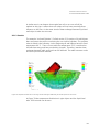
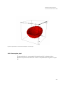
Example with inclined hemisphere and inclined rectangular
pipe (directory InclinedSphere code version 2.5)
83
Inclined hemisphere
83
Rectangular „pipe“
85
Results
88
Model reactor (directory ModelReactor, code version 2.5) 89
21
Bibliography
17.3
18
18.1
18.2
20.1.1
20.1.2
20.1.3
20.2
71
72
73
74
75
92
3
Fraunhofer-Institut für Technound Wirtschaftsmathematik ITWM
1
Authors and contributors
The project underlying this report was funded by the
Federal Ministry of Economics and Technology. Project
number: 1501369.
Sub-constractor: Becker Technologies GmbH
Project management: GRS
CoPool: Simulation software
Aivars Zemitis, Oleg Iliev, Konrad Steiner, Tatiana Gornak, Sambit Jena,
Birte Schmidtmann
CoPool: Pre-processor
Aivars Zemitis, Oleg Iliev, Konrad Steiner, Tatiana Gornak, Shrinidhi Udupi,
Vidit Maheshwari, Sandesh Hiremath
CoPool: Validation and testing
Karsten Fischer, Martin Freitag (Becker Technologies GmbH)
Walter Klein-Hessling, Martin Sonnenkalb (GRS mbH)
4
Fraunhofer-Institut für Technound Wirtschaftsmathematik ITWM
2
Overview
In this document, the usage of the software CoPool is described. The software
allows the simultaneous simulation of the fluid flow and the heat transport in
complex 3D containers. The user should be able to construct the necessary
geometries using the pre-processor software CoPrep. For the usage of this
software, see the pre-processor’s manual. In this document, we assume that
the user is familiar with the methods allowing the construction of the 3D
meshes. The used mathematical models are described apart.
In the CoPool user’s manual we explain how to install the software, how to
manage the initial and boundary conditions and how to run the code and
obtain the necessary results.
We would like to thank Karsten Fischer from Becker Technologies GmbH,
Eschborn for the proposed models for the calculation of the heat exchange
coefficient (section 13.3.1) and Martin Freitag from the same institution for
suggested improvements of the text.
New features of the CoPool version 2.5.0.
In this version, an important feature has been added to the software CoPool.
The user can shift and rotate the wall objects (see section 20.1 ).
Attention! This feature is under development and there is no guarantee that
the code is working in all cases. If this feature is used then it is necessary to
check carefully the colors of the wall boundaries (section 15.2).
3
Installation
The software is usually delivered as a package called CoPoolSetup.msi which
can be installed using the Windows Installer. To date, the installation is tested
only for Windows 7 Enterprise x64.
2
Fraunhofer-Institut für Technound Wirtschaftsmathematik ITWM
Before starting the installation of CoPool please uninstall any previous version
of CoPool, if existing . CoPool defines particular environmental variables,
therefore two different versions of the software at the same time are not
advised.
Attention! Install the code as a “normal” user and not as administrator.
During the installation the administrator’s password will be required but if the
code is installed from the administrator’s account, only the administrator can
run the program (even if the flag “Everyone” is set during the installation).
3.1
Installation resources
The software CoPool is using several open source tools which are important
either to prepare input data or for the visualization of data. Some of them are

Paraview-3.10.0 : http://www.paraview.org/

Visit 2.2.1 : https://wci.llnl.gov/codes/visit/download.html

Notepad : http://www.chip.de/downloads/Microsoft-XML-Notepad2007-v2.5_12993437.html
The first two tools can be used for the visualization of constructed geometric
objects and for viewing the simulation results. The third tool can be used to
edit xml-files. As described in the pre-processor’s manual, xml-files are the main
input for CoPool.
For using XML-Notepad-2007 directly from the GUI it is necessary to install this
tool to the standard place on your computer:
C:\Program Files (x86)\XML Notepad 2007
The other two programs, Paraview and Visit, can be placed everywhere because
they are not directly connected to CoPool.
3.2
Installation procedure
The installation procedure is the same as for usual Windows installation files. It
should be started from some “normal” user account and not from the
account of an administrator. Click the icon of the file and follow the
installation wizard. During the installation the administrator’s password will be
required.
3
Fraunhofer-Institut für Technound Wirtschaftsmathematik ITWM
After a successful installation, a CoPool shortcut should appear on the user’s
Desktop. Additionally one or several icons of directories should appear. Each
one of these directories corresponds to an example. These directories can be
copied to some other place and the user can test the program using these
examples.
In the case of a “normal” user there are no differences on which accessible
drive the project directory is created. If the user has administrator rights then in
some cases it can happen that the code has not the rights to write in the
corresponding directory. In this case the code breaks down. At first it is
necessary to test the code putting the project directory on the public space
(drive D:).
4
Workflow and using GUI of CoPool
Shortly summarized, the work with CoPool can be divided into the following
three steps:

Decision about project directory

Geometry creation and mesh generation

Simulations and viewing the results
The workflow from the user’s point of view is taken into account in the simple
graphical user interface of CoPool. Below, the workflow is explained more in
detail.
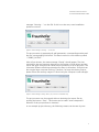
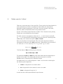
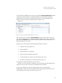
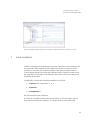
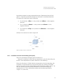
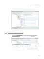
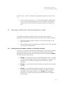
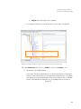
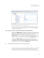
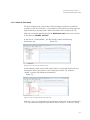
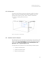
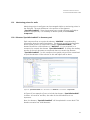
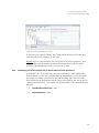
The code itself is managed from a simple GUI which appears after clicking on
the shortcut of CoPool.
4
Fraunhofer-Institut für Technound Wirtschaftsmathematik ITWM
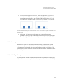
Figure 1: Graphical User Interface of CoPool
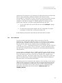
All simulations using CoPool should be organized as separate projects. Each
project should be stored in a separate directory.
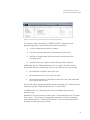
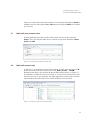
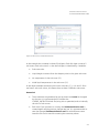
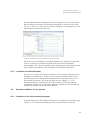
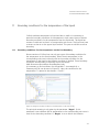
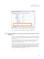
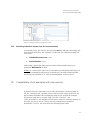
1. Open project directory using the button” Open”
By using the button “Open” the user fixes the actual simulation directory.
After clicking on “Open” a standard window appears which allows choosing
the directory with the necessary input data.
For the first tests, it is recommended to use the example projects that have
been created during the installation process on the user’s Desktop. Existing
examples are Cuboid, Sphere, Cylinder, Wall, Pool and CylindricalPool.
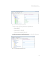
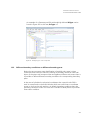
Assume we have copied the project directory “Cuboid” from the Desktop to
D:\Examples\Cuboid. Then we can select this directory for simulations.
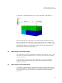
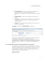
Figure 2: Window for choosing the project (working) directory, in this case D:\Examples\SpheresWalls
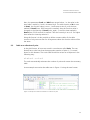
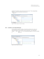
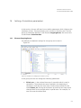
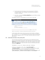
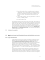
The selected project directory should be seen on the GUI.
5
Fraunhofer-Institut für Technound Wirtschaftsmathematik ITWM
Figure 3: The selected directory D:\Examples\Cuboid can be seen on the GUI
It is important to remark that the initial content of this directory consists of two
files:

DataBase.xml

Geometry.xml
In general, the project directory can contain any other files. During the preprocessor step and the simulation step additional files will be generated. If the
directory contains files with the same names as generated files then the old
ones will be overwritten without warning. The files generated by CoPool
will be discussed later.
The file “DataBase.xml” contains all material parameters which are needed for
the simulation. “Geometry.xml” contains all information which is required for
the geometry construction, the mesh generation and the solver. These two files
should be available in every project directory used with CoPool.
The geometry construction is described in the pre-processor’s manual. A
detailed description of the information needed for the solver will be discussed
later in this document.
The simulation code requires data which describe the mesh and the geometry
of different objects in an appropriate format. These data are taken from the file
“Geometry.xml” by using the pre-processor. The installed example “Cuboid” is
ready for use. If this directory is selected then we can start the pre-processor.
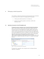
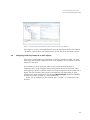
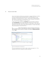
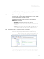
2. Starting pre-processor using the button “Preproc”
The geometry description should be stored in the file “Geometry.xml” as
described in the pre-processor’s manual. If this file is available in the chosen
directory, we can push the button “Preproc”. It is important to see the status
6
Fraunhofer-Institut für Technound Wirtschaftsmathematik ITWM
message “Running…” on the GUI. If this is not the case, some installation
problem occurred.
Figure 4: Status message "Running..." on the GUI
The pre-processor is generating all wall geometries, corresponding meshes and
also the corresponding fluid mesh. This data is stored in a sub-directory called
“COPREP_OUTPUT”.
After a few minutes, the status message “Ready” should appear. The time
required for the pre-processor depends on the number of wall objects and the
size of the grids. Fine grids can cause the pre-processor to run a long time. This
is because different searching operations are done in all meshes. Fine grids can
also require large computer memory. Therefore, for large simulation projects,
please follow the memory usage of CoPool using the computer’s task manager.
Figure 5: Status message "Ready" after a pre-processor or simulation step
The pre-processor can be stopped without obtaining the output files by
pushing the button “Stop”. This button can be used if some unexpected
behavior of the pre-processor is observed.
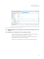
In our example project directory, the following content can be seen by now.
7
Fraunhofer-Institut für Technound Wirtschaftsmathematik ITWM
Figure 6: Content of the project directory after running the pre-processor
The content of the sub-directory “COPREP_OUTPUT” depends on the
generated geometry. The main file groups are the following:

txt-files containing step sizes for meshes

LeS-files containing geometric information for each mesh

vtk-files to visualize each mesh and test the correctness of the
boundary zones

xml-files which are used for domain-decomposition methods
Additionally the file “SubDomainFusion.xml” is created. This file contains
information about the existing sub-rooms. In this file the user can prescribe

the initial level of liquid in each sub-room

the temperature of the air in each sub-room

the initial temperature of the liquid in each sub-room if the initial level
of the liquid was not zero.
For all these values appropriate default values are already set. Further down we
will discuss the file “SubDomainFusion.xml” in more detail.
“DataBase.xml” and “Geometry.xml” are not modified during the preprocessor step.
Attention! The pre-processor creates a new “SubDomainFusion.xml” file each
time it is run. The old one is automatically overwritten. If the user changed
some default values in “SubDomainFusion.xml” then this information will be
lost after rerunning the pre-processor.
8
Fraunhofer-Institut für Technound Wirtschaftsmathematik ITWM
3. Starting simulations using the button “Simul”
If the pre-processor had no errors during the geometry generation then it is
possible to start simulations. Additional requirements are the existence of
“DataBase.xml” and that “SubDomainFusion.xml” contains correct data.
If this is fulfilled, the simulation can be started by pressing the button “Simul”.
On the GUI the status message “Running…” should appear.
Figure 7: GUI during the running process
The results of the simulation are stored in the sub-directory “results”. After a
successful simulation the structure of the project directory should be as follows.
Figure 8: Content of the project directory after a simulation.
During the simulation, a file named “logfile.txt” is created. It contains the main
information of the simulation process.
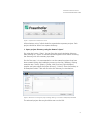
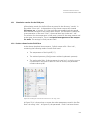
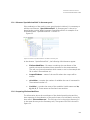
4. Starting the Xml-editor using the button “Edit”
The pre-processor and the simulation code are controlled solely through the
xml-files, though the user should carfully prepare these files. Xml-files can be
9
Fraunhofer-Institut für Technound Wirtschaftsmathematik ITWM
edited using any text editor. More convenient is to use an Xml-editor. We
propose to use XML-Notepad-2007.
If the xml-editor is installed in the standard place, it will be started
automatically by pushing the button “Edit” and the corresponding XML
Notepad GUI will appear separately. The CoPool-GUI has no influence on the
default directories which are used in XML-Notepad-2007. After initialization,
this tool proposes as default to open the file which was edited last.
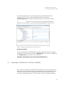
Figure 9: XML Notepad
This or another Xml-editor can also be started separately. The user edits the
necessary files and then starts again the pre-processor and the simulation
program.
5. Stopping the pre-processor or the simulation using the button “Stop”
The button “Stop” aborts the actual pre-processor or simulation run
immediately. The software can be stopped, for example, if the user notices that
some changes have to be made. After the concerning data has been edited we
can again run the pre-processor or simulation software.
The user does not need to delete files created by the pre-processor or the
simulation code. All result files are deleted automatically before starting
simulations. The pre-processor overwrites files if they already exist.
10
Fraunhofer-Institut für Technound Wirtschaftsmathematik ITWM
5
Tables used in CoPool
Tables are important parts of the input files. There can be time based tables for
some parameters (as sinks) or temperature based tables (for temperature
dependent material parameters). In all cases, the input format is the same,
therefore tables are explained without any special context.
By now CoPool allows several formats of tables. This is because some primary
formats are not excluded from the program.
The table consists on n argument values ti, i=1,...,n and n function values fi,
i=1,…,n. It is assumed that the argument values are sorted in increasing order.
Additionally, two numbers are given: Add and Scale.
Now, the true value of the parameter f for some given argument value t is
calculated by finding the value L(t) using linear interpolation from the table. If
t<t1 then L(t) = f1. If t>tn then L(t) = fn. If
and
then
()
(
)
The final value of f(t) is obtained by the formula:
f(t) = Scale*L(t) + Add
The parameters Scale and Add are some scalar values that should always be
defined for the table. The values n, fi and ti can be written in the files
DataBase.xml or Geometry.xml in different formats.
For tables there is not a special keyword “table” but the code is checking for
the following three keywords:

Value is a keyword for a constant value

N is a keyword for the number of rows in the table

Pairs is a keyword for pairs (ti ,fi)
In each case the code expects different input formats.
11
Fraunhofer-Institut für Technound Wirtschaftsmathematik ITWM
Only one of the three keywords is needed. If for example the keyword Value is
available and also the keyword N or Pairs then the keyword Value is not taken
into account.
5.1
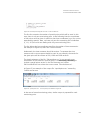
Table with one constant value
If some parameter has only constant values then we can use the keyword
Value. This is the simplest table and it consists of only three elements: Value,
Scale and Add.
Figure 10: An example of a table with constant value
5.2
Table with several rows
In this case, it is necessary to specify the number of rows using the keyword N
and then include new keywords for each row: Row1, Row2,…,RowN.
Between these tags in the xml-file the ti and fi should be written. In Figure 11,
an example of a table of this kind is shown. It is used for the description of the
intensity of a sink. In this example, the table arguments are time steps and the
function values are intensities of the sink at different time moments.
Figure 11: Example of a table with 4 rows (old format)
12
Fraunhofer-Institut für Technound Wirtschaftsmathematik ITWM
Here, the parameters Scale and Add have neutral values, i.e. the value in the
time table is scaled by 1 and is increased by 0. The table consists of N=4 rows.
In Row1, the function value is set to -1 and starts at time 0, until the time
marked in Row2 (here: 2000 seconds) is reached, then the function value is
changed to the intensity of Row2 (here: again -1) until the time marked in
Row3 (here: 2010 seconds) is reached. Then the intensity is set to 0. For higher
time values the intensity remains 0.
Using this format it is also possible to define constant tables. If the table
consists of only one row then for all argument values the function value will be
the same.
5.3
Table as a collection of pairs
In the third format, all rows are stored in one element called Pairs. The user
himself has to take care that the appropriate number of pairs (ti, fi) is noted
down for this element. The entire table should be written as a sequence in the
following way:
t1 f1 t2 f2 t3 f3 … tn-1 fn-1 tn fn
The code automatically estimates the number of pairs and creates the necessary
table.
As an example we rewrite the table seen in Figure 11 using the new format.
Figure 12: Example of a table with 4 values as a collection of pairs.
13
Fraunhofer-Institut für Technound Wirtschaftsmathematik ITWM
6
Managing material properties
For simulations of physical processes the material properties play a crucial role.
In CoPool, there are two aspects of managing material properties:
6.1

Collecting the material properties in the data base

Assigning the material properties to the fluid or walls via the
Geometry.xml file
Data base information in the file DataBase.xml
The simulation code is organized in such a way that all material parameters
needed for simulations are coming from a data base. Material properties for
fluids or walls should be collected under appropriate material names and
should be stored in the file DataBase.xml. Formally, different data base files
could be used but for each project only one data base file can be taken into
account. The file Geometry.xml has to contain the name of the data base file
(in this case DataBase.xml). Until now, simulations can be done with only one
liquid which has certain material parameters collected under an appropriate
name in the data base file. In Geometry.xml there is an element
XML::Document::DataBaseFile which should contain the complete path to the
data base file or simply the data base’s file name if it is directly in the project
directory.
Figure 13: Location of the Data base file in Geometry.xml
The data base is organized in such a way that users can always add new
materials or parameters.
14
Fraunhofer-Institut für Technound Wirtschaftsmathematik ITWM
The document DataBase.xml contains the element NumberOfMaterials which
contains the total number of included materials in the data base. Material
numbers start from 0 and for each material there is an corresponding xmlelement. The structure of a data base can be seen in the
Figure 14.
Figure 14: Structure of the material data base used in CoPool.
Each material has an element MaterialName which contains the string with
the name of the material, for example Water20.Additionally, there is a Boolean
type element IsFluid which should contain the value true if the material is a
liquid and false if it is a solid.
Recently, the code requires the following parameters for fluids:

Dynamic viscosity [kg/(m*s)]

Density [kg/m3]

Heat capacity Cp [J/(kg*K)]

Heat conductivity lambda W/(m*K)

Volume expansion used for the Boussinesq term (1/K)

Reference temperature for the Boussinesq term [°C]
An example of water parameters can be seen in
Figure 15. For the first four parameters, the previously described tables (see
section 5) can be used. The last two parameters are constants.
In the code, additional non-linear dependencies for air and liquid are
implemented. These are used to calculate the heat exchange coefficients. The
corresponding procedure is described in section 13.
15
Fraunhofer-Institut für Technound Wirtschaftsmathematik ITWM
Figure 15: Structure of water properties in the data base.
In the case of walls, only three parameters are required, so far:

Density [kg/m3]

Heat capacity Cp [J/(kg*K)]

Heat conductivity lambda [W/(m*K)]
These three parameters can be defined as temperature dependent tables using
any of the three formats for tables (see section 5).
Figure 16: Structure of material parameters for a solid.
16
Fraunhofer-Institut für Technound Wirtschaftsmathematik ITWM
The structure of the material parameters for a solid material can be seen in
Figure 16. Here, also the keyword ContactHeatTransfCoeff
can be seen. This parameter is not used for simulations anymore. The contact
heat transfer coefficient is calculated using information about the characteristic
length of the wall object, liquid velocities and the temperature. This topic is
described in section 13.2.
6.2
6.3
Remarks about input values

All input parameters are obtained from xml-files. It is not important in
which sequence the keywords for parameters are ordered in the
xml.file, only the hierarchy of data is essential.

In case that parameters are defined as tables and in the corresponding
xml-file no input data can be found then these parameters are
generated with 0 values.

In the code during the discretization process the parameter values will
be controlled. Zero values in some cases can stop the code. It is not
allowed to have a 0 density or 0 Cp. In these cases the code stops with
the message “Please check the values in the data base”.
Assigning material properties for the simulation of heat and mass transfer in the
fluid
In Geometry.xml there should be an element
XML::Document::ConfigFlow::General::MaterialName.
This element should contain a valid material name which is defined in data base
file (e.g. “DataBase.xml”). If this is not the case an error will occur. An example
how to use fluid properties for the material “Water20” can be seen in
Figure 17.
17
Fraunhofer-Institut für Technound Wirtschaftsmathematik ITWM
Figure 17: Assigning appropriate material properties to the fluid (in this case Water20)
If the input is correct, the dependencies from the data base file for the material
“Water20” will be taken for the simulation of the fluid flow and heat transfer.
6.4
Assigning material properties to wall objects
If the user is interested in the simulation of the heat transfer in walls, for each
wall object the material properties have to be assigned. This is done in a similar
way as for the fluid.
It is necessary to note down the value of the corresponding element in
Geometry.xml. For each project several wall objects can be constructed. Each
wall object in CoPool is called a compound. Each compound has an index and a
name. The file Geometry.xml contains xml-elements corresponding to each
compound. In each compound, the element MaterialType should be available
and should contain a name of a solid material. In
Figure 18, an example for the material type “Copper” of Compound1 can
be seen.
18
Fraunhofer-Institut für Technound Wirtschaftsmathematik ITWM
Figure 18: Assigning material properties to a wall object. Compound1 gets the properties of “Copper”
7
Initial conditions
CoPool is simulating time dependent processes. Therefore, initial conditions are
very important. Each variable which is taken into account requires an initial
condition. In our case, the situation becomes even more complex because
CoPool allows several sub-rooms with different levels of liquid. In other words,
the initial level of the liquid in the different sub-rooms is one of the important
conditions for the flow.
Additionally, we have the following variables for the fluid:

Velocity with components vx, vy, vz

Pressure p

Temperature T
All of them need initial conditions.
In CoPool it is possible to have several wall objects. In all wall objects we can
solve the heat conduction equation. This means that we also need initial
19
Fraunhofer-Institut für Technound Wirtschaftsmathematik ITWM
conditions for the temperature in walls. In the following sections we will
explain how to provide for CoPool all initial conditions needed.
7.1
Initial values for air and liquid temperature
The pre-processor does the room classification concerning the flooding (see
pre-processor’s manual). This information yield what parts of the container can
be flooded separately and which ones are connected. The information about
room classification is written in the file SubDomainFusion.xml. Each room has
an appropriate number (room color). Sub-rooms which connect two sub-rooms
are called link layer. So far, a link layer can only connect two sub-rooms. The
link layer is considered as a normal sub-room, i.e. the initial liquid level and
temperature should be prescribed for this sub-room, too. Each sub-room is
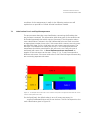
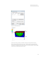
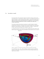
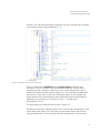
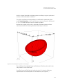
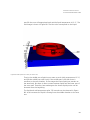
associated with some color. In Error! Reference source not found. an
xample of five sub-rooms can be seen. Colors 2, 3, 4, 5 and 6 correspond to
different sub-rooms. Sub-rooms with colors 5 and 6 are link layers because they
are connecting separate sub-rooms.
Figure 19 : An example with 5 sub-rooms. Colors 5 and 6 correspond to link layers because these sub-rooms
connect other separate sub-rooms.
For the liquid level, the default value is set to 0 (rooms are empty). In
, a typical SubDomainFusion.xml file can be seen. This file corresponds to the
room classification given in Figure 19.
20
Fraunhofer-Institut für Technound Wirtschaftsmathematik ITWM
Figure 20: Data stored in SubDomainFusion.xml
In this example the container includes 2 link layers. Each link layer connects 2
sub-rooms. Each sub-room (i.e. also the link layer) is described by 4 variables:

Sub-room color

Liquid height in meters from the deepest point in the given sub-room.

Air temperature in the sub-room (°C)

Initial liquid temperature in the sub-room (°C).
In the above example the existing sub-room colors are 5, 3, 4, 6 and 2. Since
we have 5 sub-room colors, this means that we have 5 different sub-rooms.
Attention!

Those numbers are generated by pre-processor and must be changed
by the user! It is recommended to visualize the
COPREP_OUTPUT/Fluid.vtk file (using visit or paraview) and to indentify
the color of sub-rooms.

Each time if pre-processor is running the SubDomainFusion.xml is
created again and the previous changes are lost. It is recommended to
save the changed SubDomainFusion.xml file with different name.
Later this file can be used for restoring the necessary values.
21
Fraunhofer-Institut für Technound Wirtschaftsmathematik ITWM
Remark about the initial liquid temperature
In the actual version of CoPool, the initial liquid temperature plays an important
role, even when the initial liquid level is zero. If we start to fill some sub-room
because we activated a source then automatically, the minimal water deepness,
which is 1cm in the actual version, is set in this sub-room. Therefore, at the
beginning of the filling, there is a 1 cm liquid layer in the sub-room having the
initial temperature given in SubDomainFusion.xml.
7.1.1 Initial level of the liquid
Pre-processor automatically assigns the different sub-room colors. Also, for all
initial values, some default values are written in the corresponding files. The
user should edit only these values.
For the liquid level the default value is 0 (rooms are empty).
The height of the liquid is measured from the deepest point in the sub-room to
the actual water level. For a link layer the deepest point is where it touches the
maximal water level of the lower sub-rooms it connects. There are a few more
details about link layers which should be taken into account.

For technical reasons, if we prescribe the deepness of a link layer, it
corresponds only to the part above the two sub-rooms this link layer
connects. The deepness is measured in the sub-room with appropriate
color.

If the link layer has non-zero deepness then the user should explicitly fill
the sub-rooms below. In this case, it is not necessary to know the exact
deepness of those sub-rooms. It is sufficient to give some deepness that
is larger than the real deepness of the sub-room.
22
Fraunhofer-Institut für Technound Wirtschaftsmathematik ITWM

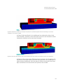
An important restriction: until now, each link layer can only connect
two sub-rooms. If Pre-processor generates link layers which connect
more than two sub-rooms, the resulting SubDomainFusion.xml file is
not usable for simulations with CoPool now (see Figure 21 on the left).
Figure 21: On the left the link layer (sub-room 4) connects 3 sub-rooms (1, 2 and 3). On the right two link
layers can be seen. The link layer 5 connects sub-room 1 and sub-room 4. The link layer 4 connects sub-room
3 and sub-room 4.

In this case, it is necessary to change the geometry. One has to
generate a small link layer in between the connected rooms (see Figure
21 on the right). This sub-room configuration is allowed in CoPool.
7.1.2 Air temperature
Each sub-room (also link layers) can have different air temperatures. The air
temperature only has a meaning if the room is not filled with liquid. The given
air temperature can be taken into account for the boundary conditions of the
liquid and also for the walls. Each liquid level “knows” which air temperature is
above the liquid.
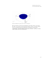
7.1.3 Initial liquid temperature
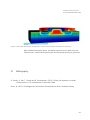
For each sub-room we can prescribe different initial temperatures of the liquid.
In Figure 22 we see an example where the temperature in sub-room 1 is 30 °C,
23
Fraunhofer-Institut für Technound Wirtschaftsmathematik ITWM
in sub-room 2 the temperature is 20 °C and in sub-room 3 we have 40 °C.
Figure 22: Example with non-zero initial height in the link layer and different temperatures in sub-rooms
Here, the liquid levels of sub-room 1 and 2 have been set to 6. Starting at the
deepest point, i.e. at -14, the liquid should be filled till -8 but we can see that if
the prescribed deepness of sub-rooms is larger than the real deepness, the
underlying sub-rooms are simply filled up.
7.2
Initial values for the flow variables
The initial values for the flow variables as the velocity components vx, vy, vz and
the pressure p are automatically set to 0. Until now, the user cannot change
these initial values.
In the model we work with the reduced pressure (i.e. without hydrostatic
pressure). The full pressure is the sum of the calculated pressure and the
hydrostatic pressure.
7.3
Initial values for wall temperatures
The walls must be described as separate wall objects (separate compounds) in
the Geometry.xml file. The temperature in wall objects can only be simulated if
for this compound a correct LeS-file and a correct step-size file have been
generated.
24
Fraunhofer-Institut für Technound Wirtschaftsmathematik ITWM
The initial temperature of a wall compound must be defined directly in
Geometry.xml. For each compound there should be an element
InitialTemperature where the initial temperature of the wall is specified.
In
Figure 23, it can be seen how the initial temperature is
defined for Compound1. In this case the initial temperature is set to 50 °C.
Figure 23: Setting the initial temperature for Compund1 to 50 °C
Important remark:
In order to simulate the wall temperature and to take into account the initial
temperature of the wall, the element “WallIsActive” has to be set to true. For
the Compound1 the full path of this element is:
FileInput::VoxelCompounds::Compound1::WallIsActive.
8
Boundary conditions for the flow variables
Since CoPool is solving the 3D Navier-Stokes equations, all flow variables (the
velocity components vx, vy, vz and the pressure p) need appropriate boundary
conditions. One part of these boundary conditions is set automatically and
cannot be changed by the user. The other part of these boundary conditions
25
Fraunhofer-Institut für Technound Wirtschaftsmathematik ITWM
can be changed by the user. We recommend to do it only for experienced
users.
The boundary conditions for the liquid flow are described in Geometry.xml
under XML::Document::BoundFlow.
Historically, the boundary of the fluid mesh was separated in three parts: Inlet,
Outlet and Solid. We can find these parts in the example file Geometry.xml.
Figure 24: Description of flow boundary conditions in Geometry.xml
So far, pre-processor does not provide a possibility for defining the Outlet part
of the boundary. Therefore, only the Inlet and the Solid boundary conditions
are used. The Outlet’s part is available in Geometry.xml but must be empty. The
Inlet boundary part corresponds to the free boundary and the Solid boundary
part to the contact zone between the liquid and the wall parts. Until now, for
the pressure and the velocity on all wall parts, the same conditions will be
applied – automatically or by user input.
8.1
Boundary conditions for velocity
8.1.1 Notation for faces
Each voxel has 6 faces. In the code each face has an appropriate name. These
names are used if special boundary conditions should be applied on voxel
26
Fraunhofer-Institut für Technound Wirtschaftsmathematik ITWM
boundaries oriented in some prescribed directions. Remember that the fluid
mesh is a Cartesian mesh and the faces are oriented in coordinate directions.
The names for voxel faces are the following:

For X-direction: vfEast – in the positive and vfWest – in the negative
direction

For Y- direction: vfNorth – in the positive and vfSouth – in the
negative direction

For Z-direction: vfTop in the positive and vfBottom – in the negative
direction.
All faces of a voxel can be seen in Figure 25.
Figure 25: Names of faces of a fluid voxel
8.1.2 Conditions on the free boundary (Inlet part)
We do not recommend changing these conditions. In
Figure 26, conditions for the velocity components on the free boundary can
be seen. The interpretation of these conditions is the following:
Due to the fact that in CoPool the Inlet corresponds to the free boundary, the
conditions on the Inlet part can only be used on the top surface of the fluid
voxel. In the code, the top surface (face) of the fluid voxel is called “vfTop”. On
the free surface we set the normal derivatives of the horizontal velocity
components to 0. This is achieved by setting the boundary type Element
“Btype” to 1 (zero flux).
27
Fraunhofer-Institut für Technound Wirtschaftsmathematik ITWM
For the vertical velocity components, the boundary type is set to 0. This means
that the velocity component will be directly assigned. In the xml-file the value
for “Vz” is set to 0. In the code, this value is changed in correspondence to the
mass balance in the actual sub-room.
Figure 26: Conditions for velocity components on the free boundary
Heretofore, the mass balance is calculated based on the activities of sinks and
sources. In the case of overflow artificial sinks and sources are defined
automatically. This is just one example which already shows that changes in the
Inlet conditions can lead to some problems in the simulation algorithm.
8.1.3 Conditions on walls (Solid part)
Up to now, two types of boundary conditions for the velocity components can
be applied on solid walls. If “Btype” is set to 0 then an explicit value for the
velocity component is expected. Inserting the Value 0 corresponds to the noslip boundary condition. The other possibility is to set “Btype” = 3. This
boundary condition corresponds to the slip-condition. The normal velocity
component will be set to 0, and a zero gradient condition for the two velocity
components parallel to the wall will be applied.
8.2
Boundary conditions for the pressure
8.2.1 Condition on the free boundary (Inlet part)
As mentioned above, this condition should not be changed. The boundary type
“Btype” is 0 on the free boundary (the pressure value should be directly
28
Fraunhofer-Institut für Technound Wirtschaftsmathematik ITWM
assigned). The value for the pressure must be set to 0. The corresponding
fragment of the xml-document can be seen in
Figure 27.
Figure 27: Pressure condition on the free boundary
8.2.2 Condition on the walls (Solid part)
On the walls the pressure condition should also be fixed. In this case, the
normal derivative of the pressure function should be 0. This means that
“Btype” = 1 and “Value” = 0. The corresponding fragment of xml-file is shown
in
Figure 28.
Figure 28: Pressure condition on the walls
29
Fraunhofer-Institut für Technound Wirtschaftsmathematik ITWM
9
Sources and sinks
Sources and sinks are the key input parameters to trigger fluid flows in CoPool..
The user can define several sinks and sources in the fluid domain. For the
description of sinks and sources in CoPool, only one type of element exists in
the xml-file. It is called Sink. If the intensity of a sink is positive, we will have a
sink, if the intensity is negative, we have a source.
In the xml-file, within the Element FlowParam, there should be an Element
called NumbOfSinks. The corresponding value will tell the code how many
sinks and sources will be used in the current run. If this value is 1 then only the
information about Sink1 will be used during simulations, no matter how many
sinks are described in the xml-document.
In
Figure 29 an example of a source can be seen. We can see
that it is a source and not a sink because the intensity is negative. For sources
the temperature must be defined. Therefore, the element TemperatureAvail
is set to true.
Figure 29: An example with a source description
The source temperature in this case is taken constant and equal 10 °C. The
intensity of this source is defined as a table using pairs.
30
Fraunhofer-Institut für Technound Wirtschaftsmathematik ITWM
9.1
Parameters characterizing sinks and sources
9.1.1 Element: TemperatureAvail
This parameter can be removed in the future. It indicates if the temperature for
this construct is available or not. Until now, it is necessary to set this parameter
to “true” if we want to define a source (negative intensity) and it should be set
to “false” if we want to define a sink (positive intensity). In this case, the
temperature will not be used even if some value for the temperature is
available in the xml-file.
9.1.2 Element: HasToBeMoved
As CoPool can start simulations with empty sub-rooms, it is necessary to be
able to move a source to the water level. Each sink (or source) has the
parameter “HasToBeMoved”. If the value is set to “true” then this sink (or
source) will always be mapped to the upper layer of the liquid. In other words,
the sink or source will always be moved together with the free boundary. It
means that also a shifting in x-y-plane will be done if shifting in z-direction
alone leads to some position outside the fluid domain.
If “HasToBeMoved” has the value “false” and the intensity is positive (real sink)
then this sink will work only if it is underneath the liquid level.
If “HasToBeMoved” has the value “false” and the intensity is negative (real
source) then two different scenarios at each time step can happen:

If the original position of this source is below the actual free boundary
then the source remains at the original position.

If the original position is higher as the actual free boundary then the
source will be projected to the free boundary.
There are no restrictions to this parameter in the case of several sub-rooms and
several liquid levels.
31
Fraunhofer-Institut für Technound Wirtschaftsmathematik ITWM
9.1.3
Element: CountSinksOfThisType
This parameter was used in earlier versions. Currently, the value of this
parameter must be set to 1.
9.1.4 Element: Temperature
This parameter has a meaning, if “TemperatureAvail” is set to “true”. In the
case of sources, the source temperature is used in the heat equation for the
fluid.
The source temperature can be constant or also time dependent.
In the case of a constant source temperature it is possible to assign the
temperature value to the sink with appropriate index directly. In the case of the
Sink1 we should assign the temperature value to the xml-element
“Document::ConfigFlow::General::FlowParam::Sink1::Temperature”.
An example of assigning the constant value 10 °C can be seen in Figure 30.
Figure 30: Assigning a constant temperature value (10 °C) to the Sink1
In more general case the temperature is time dependent. Therefore, also time
tables for the temperature of sources are allowed. An example is shown in
Figure 31.
Figure 31: Temperature of the source as a time table
32
Fraunhofer-Institut für Technound Wirtschaftsmathematik ITWM
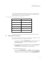
The temperature is defined as a time table using “Pairs”. In the pair the first
value corresponds to the time and the second value to the temperature. The
corresponding table is shown below (see Table 1).
Table 1: Time table for the source temperature corresponding to Figure 31
Time [s]
Temperature [°C]
0
10
50
20
100
30
150
40
200
100
300
10
In this case all 3 formats for a time table described in section 5 can be used.
9.2
Positioning of sinks and sources
The positioning of sinks in 3D structures is a difficult task. Therefore, in CoPool
there are some tools which allow simplifying this work.
1. For each sink, a parameter SubRoomColor should be prescribed. This
color must correspond to the sub-room classification written in
SubDomainFusion.xml.
2. Each sink should have a coordinate list which is stored in the parameter
Coordinates0. The parameter should contain 3 numbers. They are
corresponding to the coordinates in x, y and z direction.
Now, different situations can occur.

Assume that HasToBeMoved is set to false. In this case, the position
of the sink is fixed. If the coordinates of the parameter Coordinates0
correspond to a point in the sub-room with color SubRoomColor then
33
Fraunhofer-Institut für Technound Wirtschaftsmathematik ITWM
the sink is positioned in this place. If the coordinates of sink from
Coordinates0 do not correspond to some internal point of the subroom with the color SubRoomColor, the sink is shifted horizontally to
the closest point of the sub-room with color SubRoomColor. If it is not
possible then the sink will not work. In any case, the sink can only work
if the water level is above its position. The sink will remain at this point
independent of the free boundary level. For sources (the intensity is
negative) the shifting also in the vertical direction will happen if the
original position is above the actual liquid level (see 9.1.2). In this case
the shifting is not only inside the sub-room with color SubRoomColor.
The projection will be done also to sub-rooms below this one if needed.

9.3
Assume that HasToBeMoved is set to true. In this case, the source
moves from its original position to the closest point of the
corresponding free surface. It means that horizontal and vertical shifting
of the source will be done automatically.
Prescribing intensities for sinks and sources
Intensities of sinks and sources are prescribed using tables (cf. section 5).
Currently, all three formats can be used. In Figure 29 an example with the third
table format for source intensities can be seen.
10
Turbulent parameters
The recent CoPool version allows the user to change the viscosity of the liquid
in the file Geometry.xml without changing the value in the file DataBase.xml.
There is the possibility to define different values for horizontal and vertical
viscosity and/or for horizontal and vertical heat conductivity. Recently, these
parameters can only be constant values (constant tables). The defined values
will be added to the original values from the data base.
To use turbulent parameters, it is necessary to include in Geometry.xml for the
element FlowParam a new child Element TurbParameters (see
Figure 32).
34
Fraunhofer-Institut für Technound Wirtschaftsmathematik ITWM
Figure 32: TurbParameters as a new child element to FlowParam
In this version, the turbulent viscosity and the turbulent conductivity coefficients
are included. We will describe viscosity and heat conductivity separately.
10.1
Turbulent viscosity
Turbulent viscosity will be represented as a new child element TurbViscosity of
the element TurbParameters.
TurbViscosity contains again two child elements: Horizontal and Vertical.
Each of these elements should be represented as a table (see section 5).
In the example in Figure 33 we have set the horizontal turbulent viscosity to 0
[kg/(m*s)].The vertical turbulent viscosity is set to 10 [kg/(m*s)]. This means that
the actual viscosity in the horizontal direction will be equal to original value
found in the data base. The vertical viscosity used for simulations consists of the
viscosity found in the data base, increased by 10 [kg/(m*s)].
35
Fraunhofer-Institut für Technound Wirtschaftsmathematik ITWM
Figure 33: Example of using turbulent viscosity
10.2
Turbulent heat conductivity for the liquid
The element TurbParameters can contain a second child element called
TurbConductivity (see
Figure 34).
Figure 34: TurbConductivity as a child element of TurbParameters
TurbConductivity contains again two child elements: Horizontal and
Vertical. Similarly as in the case of turbulent viscosity, each of them has to be a
table defining the values of conductivity which will be added to the original
conductivity found in the data base.
36
Fraunhofer-Institut für Technound Wirtschaftsmathematik ITWM
11
Boundary conditions for the temperature of the liquid
CoPool simulates temperature in liquid and also in walls. It is necessary to
prescribe boundary conditions for temperature in both cases. Here we discuss
boundary conditions for the temperature from the liquid side. The liquid has
contact to walls and to the air in corresponding sub-rooms. The liquid can have
a contact to the air on the upper liquid surface. This part we call also as a free
boundary.
11.1
Boundary conditions for the temperature on the free boundary
Recent versions of CoPool can use only two types of boundary conditions for
the temperature on the free boundary. Either the air temperature in the
corresponding sub-room is directly used as a boundary condition for the
temperature in the liquid or the isolation condition is applied. Those boundary
conditions are described in Geometry.xml in the section
XML::Document::BoundFlow::BoundaryPart::Inlet.
It is necessary to find conditions for the variable T. An example of a
Geometry.xml file can be seen in Figure 35. Here, the condition for the
temperature T is placed in the element “Cond2”.
Figure 35: Setting the boundary conditions for the temperature on the free boundary
The principal meaning is only given by the parameter “Btype”. If this
parameter is set to 0 then the air temperature in the corresponding sub-room is
used for the boundary condition. If “Btype” is set to 1 then the isolation
37
Fraunhofer-Institut für Technound Wirtschaftsmathematik ITWM
condition for the temperature in the liquid will be applied on the free
boundary, i.e. no heat conduction between water and air.
If Btype = 4 then in this case heat exchange between liquid and air is
simulated. Here the same method is used for calculation of heat exchange
condition as in the case of wall and liquid (see section 13.3.1). Instead of wall
parameters here the liquid parameters and properties are used. The
characteristic length is calculated as square root of the corresponding free
surface area. Remember, CoPool is not simulating the heat conductivity in air.
Only prescribed air temperature and velocity values can be taken in to account.
The possibilities of defining time tables for air are described in section 12.
11.2
Boundary conditions for the temperature next to walls
Boundary conditions for the temperature of the liquid which is in contact with
walls are set fully automatically. The boundary face of a fluid region might be
in contact to several boundary faces of wall objects. These relationships are
calculated automatically. Recently, it is assumed that one face of a wall voxel
has a relationship to only one fluid region face. As a boundary condition for
the fluid face the heat flux condition is used. For the given fluid face on the
boundary, the sum of all wall heat fluxes related to this fluid face is evaluated.
This flux is then used as a boundary condition. In section 13, more details on
the boundary conditions of the wall side are given.
12
AirParameters in Geometry.xml
In CoPool, the user has several possibilities to define air conditions in subrooms. This can be done in two ways: The simplest case is to define a constant
air temperature in the sub-rooms. For this purpose, the file
SubDomainFusion.xml is suitable (see section 7.1.2 ).
By now, it is possible to give more detailed information about the air flow. This
can be done by adjusting the element AirParameters in Geometry.xml.
Remember that the pre-processor estimates how many sub-rooms are available
in the constructed geometry and automatically creates the file
SubDomainFusion.xml. For each sub-room, a default value for the air
temperature is prescribed. The user can edit these default values in
SubDomainFusion.xml, if needed.
38
Fraunhofer-Institut für Technound Wirtschaftsmathematik ITWM
If it is not sufficient to have only constant air temperatures for the sub-rooms, it
is necessary to include the new element AirParameters in the file
Geometry.xml.
In recent versions there are the following rules concerning the air parameters:
12.1

If there is no element AirParameters in Geometry.xml then the code
obtains information about the constant air temperature from the file
SubDomainFusion.xml.

If the element AirParameters is available in the Geometry.xml, the
information about air temperatures found in SubDomainFusion.xml is
not taken into account.

If the user decides to include the element AirParameters in
Geometry.xml then the information about air temperatures should be
given for each sub-room recognized in SubDomainFusion.xml.
Structure of AirParameters
The structure of this element will be explained on the basis of the following
example (see
Figure 36).
Figure 36: AirParameters for 3 sub-rooms
In this case, air parameters are prepared for 3 sub-rooms.
Attention! The number of sub-rooms should exactly correspond to the total
number of sub-rooms in SubDomainFusion.xml. This means that before the
39
Fraunhofer-Institut für Technound Wirtschaftsmathematik ITWM
element AirParameters is prepared, it is necessary to run the pre-processor
and to find out the number of sub-rooms by studying the file
SubDomainFusion.xml (see section 15.1.1).
12.2
Structure of AirParameters for a given sub-room
For each sub-room, we have to describe the air temperature and we can also
describe the velocity values in the given sub-room.
All parameters should have the same structure. The child elements of
SubRoom* are the following:
12.3

RoomColor: contains the color of the given sub-room,

Temperature: contains the time table for the air temperature in the
sub-room

Velocity: contains again 3 child elements: Vx, Vy and Vz. Each of
these elements contains time tables for the velocity components.
Time tables for the air temperature and the air velocities
For the input data, the different tables presented in section 5 are used.
In
Figure 37, the time table for the temperature and for the
velocity component “Vx” of the sub-room with room color 4 can be seen.
Figure 37: Time tables for the temperature and the velocity component “Vx” in the sub-room with color 4
In this example, the air temperature in the sub-room with color 4 is growing
linearly starting from 50 °C at t=0 seconds until it reaches 100 °C at 1000
40
Fraunhofer-Institut für Technound Wirtschaftsmathematik ITWM
seconds. Once t =1000 s is reached, the temperature remains constant (100
°C).

13
The air velocity component “Vx” is also linearly growing, starting from
5 m/s at t=0 seconds and achieving 10 m/s at t=500 s. After having
reached 10 m/s at 500 seconds, the velocity remains constant (at 10
m/s).
Boundary conditions for the heat equation in walls
It is necessary to define boundary conditions for each wall compound
separately. There are two different ways for defining the boundary conditions:
13.1

Define the same boundary condition for the whole boundary of the
given compound.

Define different boundary conditions on different parts of the boundary
for the given wall compound.
Setting the same boundary condition on the whole boundary
In CoPool, it is possible to describe three different types of boundary conditions
for the heat equation in walls. The type of boundary conditions should be
described for each wall compound individually using the xml-element BcType.
The three possible conditions are:

BcType = 0 means that the air or liquid temperature close to the wall
is used as the boundary condition for the temperature in this wall. This
feature can be convenient if only the heat conduction in walls is
simulated.

BcType = 1 means that the wall is isolated. No heat flux from outside is
available.

BcType = 4 is the default boundary condition. In this case the heat
exchange coefficient is estimated. This kind of boundary condition is
discussed in more detail in section13.2. If BcType is not explicitly
defined for a compound, this type of boundary condition is applied
automatically.
41
Fraunhofer-Institut für Technound Wirtschaftsmathematik ITWM
An example of a Geometry.xml file with explicitly defined BcType can be
found in Figure 38. In this case, BcType = 0.
Figure 38 : Setting BcType = 0 for Compound1
13.2
Different boundary conditions on different boundary parts
During the pre-processor step classification of possible sub-rooms is done.
These sub-room colors are used for coloring of boundary voxels for each wall
object. If the given wall compound has as neighbors different sub-rooms then it
is possible to define different boundary conditions for corresponding boundary
parts.
In the case of cylindrical or spherical coordinates also a special color 300 is
used. It corresponds to the artificial holes which are used close to coordinate
center or close to the pole position. As default boundary conditions here the
symmetry condition is used. The user can if needed in these places to prescribe
some other condition.
42
Fraunhofer-Institut für Technound Wirtschaftsmathematik ITWM
Figure 39: Setting different boundary conditions for a wall compound
13.3
Boundary conditions for the temperature on contact faces with liquid in the case
BcType = 4
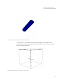
13.3.1 Method for the calculation of the heat exchange coefficient
If the wall boundary is below the liquid level then a simplified heat transfer
correlation, explained below, is implemented in CoPool.
Here we describe the main principles used for modeling the heat transfer
between the fluid and the heat conducting wall.
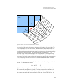
In Figure 40, the schematic view of a fluid mesh and a wall mesh is given.
43
Fraunhofer-Institut für Technound Wirtschaftsmathematik ITWM
fluid
wall
Figure 40: Schematic view on the fluid mesh and the wall mesh
The dotted red line with the red cross indicates the location of the variable Twall
of the temperature of the wall surface. Remember that the wall boundary can
be represented also in curvilinear coordinate systems. Therefore, the wall
boundary can be approximated more exact in comparison to the corresponding
boundary from the liquid side. The associated water temperature Tfluid is
calculated using a weighted average of the temperatures in the neighboring
fluid cells, which are indicated by black crosses. For the weights, the inverse
distances of the black crosses to the red cross can be used. In the recent version
of the software the closest fluid voxel is taken and the temperature from this
voxel is used as Tfluid.
The heat flow normal to the wall surface element is indicated by the dashed
red line. It is calculated as follows:
(
)
is the heat flow, is the area of the wall surface element in
and α is
the heat transfer coefficient in
. The heat flow from the wall has to be
the same as the heat flow to the neighboring fluid cells (energy conservation).
We assume that each wall face is related to only one appropriate fluid cell. It
44
Fraunhofer-Institut für Technound Wirtschaftsmathematik ITWM
means that the wall face has a heat exchange only with one fluid cell. But it
does not mean that one fluid cell has a heat exchange only with one wall cell.
One fluid cell can have interaction with several wall cells and even with several
wall objects. The sum of heat fluxes trough all related wall faces is used as a
flux boundary condition for this boundary fluid cell.
In order to calculate the heat transfer coefficient α, a number of other terms
must be calculated. First, the orientation of the normal vector of the wall
surface element must be determined. The normal vector points into the fluid. If
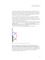
the angle between the vertical and the normal vector is less than 45° (i.e. if the
normal is in region a, in the blue part in
Figure 41), then the wall surface area element is approximately horizontal
(ceiling). If the angle is between 45° and 135° (the normal vector is in region b,
in the red part in
Figure 41), then the element is
approximately vertical (side-wall). If the angle is between 135° and 180° (the
normal vector is in region c, in the green part in
Figure 41), then the element is approximately horizontal (floor).
a
b
c
Figure 41: Schematic picture of possible orientations of normal vectors
Now, the characteristic geometric length must be determined for heat
transfer. This parameter is used in formulas (13.1) and (13.2). For vertical
cuboid or cylinder faces is the height of the surface. For horizontal cylinder or
sphere faces is the diameter. For horizontal cuboid faces is the smaller one
of the lengths of the two sides. This information must be generated by the user
and stored in Geometry.xml file for each wall mesh. More in details this
procedure is described in section 13.3.2.
45
Fraunhofer-Institut für Technound Wirtschaftsmathematik ITWM
Here, “Vertical” means the direction along the gravitational acceleration. The
characteristic length refers to the full dimension of the geometric object, not
to the dimension of the wall surface element obtained by discretization.
Next CoPool calculates some material properties like  (
, thermal
conductivity of water),  ([m²/s], kinematic viscosity of water) and ([m²/s],
thermal diffusivity of water). These property functions are evaluated at Tmean, the
average temperature between fluid and wall: Tmean = ½ (Tfluid + Twall).
We also need the thermal expansion coefficient [1/K] of water which is
obtained by differentiation of the temperature-dependent density ( ) at
constant pressure:
In CoPool, a table of material properties for water and air is implemented. In
this table the values for
at different temperatures can be found.
Virtually, the data are independent of the pressure. (The data for can also be
used to calculate buoyancy forces in the equation of motion using the
Boussinesq approximation). The following parameters are important for further
calculations:
is the thermal diffusivity,
is the Prandtl number.
The Grashof number, relevant for natural convective heat transfer, is calculated
as
|
|
(13.1)
46
Fraunhofer-Institut für Technound Wirtschaftsmathematik ITWM
where
is the gravitational acceleration.
The Nusselt number for natural convective heat transfer under fully developed
turbulent conditions is given by the correlation
(
)
⁄
For forced convective heat transfer, a characteristic water flow velocity along
the surface must be estimated. In most cases, the velocity component normal
to the wall surface element is close to zero. The absolute velocity in the center
√
of neighboring fluid cell
is a suitable estimate.
The Reynolds number is
(13.2)
The Nusselt number for forced convection heat transfer is given by the Colburn
correlation
⁄
The actual Nusselt number is the maximum of the values for natural and forced
convection:
{
}
The heat transfer coefficient is calculated as
The simple correlations for natural and forced convective heat transfer given
above were taken from (Elsner, 1973) .
13.3.2 Prerequisites for the calculation of α
During assembling the matrix for heat conductivity in walls, the code should go
through all wall voxels. As can be seen from equations for the calculation of ,
given in section 13.3.1, the global information of the object (characteristic
length L) is required. The user should give information needed to calculate L.
47
Fraunhofer-Institut für Technound Wirtschaftsmathematik ITWM
This information must be explicitly written in Geometry.xml for each wall
object.
Here, the question could arise why the user shall write this information
explicitly. The answer is the following: Each wall object can be constructed
using different basic prototypes and Boolean operations. By now, there is no
tool given in the pre-processor, which automatically extracts the necessary
information about the characteristic length L.

Information for spherical objects
For spherical objects, only the radius of the sphere is needed. It is
necessary to write this value in the element WallGrid of the
corresponding compound.
Figure 42: Setting the information about the characteristic length of a spherical object
In the example seen in
Figure 42, the radius
used as characteristic length for the sphere is set to 15 m.

Information for cylindrical objects
Because in the general case the cylinder can have different inclinations,
the user has to provide more information for cylindrical objects:

CenterLine_P gives the orientation vector of the cylinder

Radius gives the radius of the cylinder
48
Fraunhofer-Institut für Technound Wirtschaftsmathematik ITWM

Height gives the height of the cylinder
An example of data for a cylindrical object can be seen in Figure 43.
Figure 43: Information needed to calculate the characteristic length of cylindrical objects
Here the CenterLine_P = <0 0 -1>, Radius = 0.8 m and Height = 4 m.

Information for parallelepipeds
In this case, the three parameters Lx, Ly and Lz are required. The actual
version of the pre-processor cannot generate inclined boxes. This means
that the faces of the parallelepiped have to be parallel to the coordinate
planes. An example of parameters for a parallelepiped can be seen in
Figure 44.
49
Fraunhofer-Institut für Technound Wirtschaftsmathematik ITWM
Figure 44: Parameters to calculate the characteristic length for the case of a parallelepiped
For the parallelepiped in this case Lx = 4 m, Ly = 4 m and Lz = 2 m.
13.4
Boundary conditions for the temperature on the contact faces with air in the case
of BcType = 4
The estimation of the heat exchange coefficient is done in the same way as in
section 13.3.1 except that all material and flow characteristics have to be for air
instead of fluid.
CoPool does not simulate air. In the future all necessary information will be
obtained from COCOSYS. Until now, the user can define appropriate
conditions on air using input files.
In some of the next versions of CoPool, the boundary conditions on the contact
faces with air will be treated similarly as described in section 13.3.1. Recently,
in the case of contact with air, the value of air temperature is taken as a
boundary condition. The air temperature for each sub-room should be fixed in
the file SubDomainFusion.xml (see section 7.1.2).
50
Fraunhofer-Institut für Technound Wirtschaftsmathematik ITWM
14
Setting of simulation parameters
In this section, the user will learn how to define parameters which influence the
simulation process. These parameters can be found in Geometry.xml. The first
group of parameters belongs to the Element SteppingParam, the second one
to the Element LinSolvParams.
14.1
Element SteppingParam
An example of parameter settings for this group can be seen in
Figure 45.
Figure 45: Parameters for managing the simulation process
In this group the user can change the following parameters:

DTmin_sec – is the minimal time step (in seconds) which is used in
simulations. The minimal time step is applied in the beginning of
simulations, and then the time step is continuously increased to the
value DTmax_sec. During the simulation process the time step can be
changed back to the minimal value in special cases. For example, if a
new sub-room should be filled.
51
Fraunhofer-Institut für Technound Wirtschaftsmathematik ITWM

DTmax_sec – is the maximal time step (in seconds) which is used in
simulations.

DTouput_sec – is the time interval (in seconds) between the outputs of
result-files.

Tend_sec – is the time (in seconds) when the simulations stops.

MaximumStepCount – is the total number of time steps which are
allowed. If the actual time step count becomes larger than this value,
the simulation is stopped.
In the actual version, the user should not change the values for:
14.2

AdaptTimeStep, (currently only false is allowed)

CFLcoeff.
Element LinSolvParams
In this element, only two parameters are available.
14.2.1 Relative residuum LSTol
LSTol is the tolerance of the relative residuum at which the linear solver
delivers the numerical solution of the linear system. For all linear systems, the
same parameter is used (default value: 1.e-9). The corresponding data structure
in Geometry.xml can be seen in
Figure 46.
52
Fraunhofer-Institut für Technound Wirtschaftsmathematik ITWM
Figure 46: Setting parameters for the linear solver and DD-method
Formally it would be possible to set different tolerances for each equation. In
this case for all equations the same tolerance is used. Therefore, we suggest
not increasing this parameter.
14.2.2 Iteration number in domain-decomposition method DDIterations
The parameter DDIterations is important for the domain-decomposition (DD)
method. This method is used for solving the heat equations in walls. In CoPool
a version of overlapping DD-method is implemented. The parameter
DDIterations tells how much iteration during one time step should be done.
The default value is 1. This value is set automatically if this parameter is not
available in Geometry.xml. In Figure 46 the parameter DDIterations is set to 3.
The parameter DDIterations has a meaning only for wall objects with
overlapping regions. For wall objects which are fully separately, iterations are
not needed. For these objects additional iterations are not applied and this is
independently from the actual value of DDIterations.
15
Checking the output files of the pre-processor
CoPool can solve complex hydrodynamic and heat problems. But it can happen
only if the geometry construction, meshing, setting initial and boundary
conditions are done correctly. Pre-processor of CoPool is generating geometry,
53
Fraunhofer-Institut für Technound Wirtschaftsmathematik ITWM
creating the discretization of this geometry and doing partitioning of boundary
cells for setting boundary conditions. Because a lot of work is done
automatically, it is important to check if all steps by the pre-processor are done
correctly. The pre-processor is preparing files in vtk-format which can be
visualized. These files are written in COPREP_OUTPUT sub-directory of the
actual project directory. Vtk-files are generated following the rules:

For the fluid mesh only one vtk-file with the name Fluid.vtk is always
generated

For each wall compound a separate vtk-file is generated. The name
convention for these files: <Compound name>.vtk.
In the following sub-sections these files are discussed more in details.
15.1
File “Fluid.vtk”
The pre-processor generates different files on the base of the file
Geometry.xml. Those output files are stored in a sub-directory of the project
directory named COPREP_OUTPUT (see section 4). One type of the generated
files are vtk-files which can be visualized using a visualization tool as
“Paraview” or “Visit”. The generated vtk-files in the COPREP_OUTPUT directory
can be divided in two groups. The file “Fluid.vtk” contains information about
the fluid mesh. All other vtk-files correspond to wall compounds and describe
wall geometries.
It is important to understand that in COPREP_OUTPUT written vtk-files do not
give the exact size of objects. They contain additional layers of voxels. The real
size of the object can be seen if the filter for internal color is applied in the
visualization software. The internal voxels have to be covered with at least one
layer of boundary voxels. These boundary voxels will be used for creating of
boundary faces in the discretized geometries.
Boundary voxels must characterize the medium of the boundary. In the case of
walls boundary voxels must contain the color of corresponding fluid sub-room.
In the case of overlapping boundary parts the boundary voxels positioned in
some other wall objects must contain a special color for overlapping parts.
Information about wall colors can be found in WallColor.xml from
COPREP_OUTPUT.
54
Fraunhofer-Institut für Technound Wirtschaftsmathematik ITWM
If we read the file “Fluid.vtk” and visualize the data using “Pseudocolor”
Compound_100, then after clipping and applying a threshold for the variable
Compound_100, it is possible to get information about different groups of
voxels in “Fluid.vtk”. The file “Fluid.vtk” should correspond to the file Fluid.LeS
which is used to construct the simulation mesh in the simulation software.
On the base of the example SphereWalls which is delivered with the software
we will now show which information can be obtained from the fluid mesh.
15.1.1 Sub-rooms in fluid mesh
The pre-processor automatically classifies the sub-rooms in a 3D geometry. This
classification gives information about the possible filling scenarios. Separate
sub-rooms can be filled separately. Sub-rooms which connect other sub-rooms
are called link layers. Information about sub-room colors used in “Fluid.vtk” is
stored in the file “SubDomainFusion.xml”. It is important to check before
simulations that the room classification is done correctly.
In the example “SpheresWalls”, the content of SubDomainFusion.xml is shown
in
Figure 47.
Figure 47: Content of SubDomainFusion.xml for the example "SpheresWalls"
It can be seen that three sub-rooms with sub-room colors 2, 3 and 4 exist. The
sub-rooms with color 2 and 3 are separate; they are connected by the subroom having the color 4, which is a link layer.
Using the file “Fluid.vtk”, we should be able to visualize these three sub-rooms.
It is important that the threshold values are set between 2 and 4 (see
Figure 48).
55
Fraunhofer-Institut für Technound Wirtschaftsmathematik ITWM
Figure 48: Threshold settings in Visit
Figure 49: Fluid voxels in the example "SpheresWalls" obtained by Visit using threshold and clipping
Now, all internal fluid voxels can be seen: The blue voxels correspond to the
sub-room 2, the green ones to the sub-room 3 and the red part is the link layer
(sub-room 4) connecting both sub-rooms.
56
Fraunhofer-Institut für Technound Wirtschaftsmathematik ITWM
15.1.2 Walls in fluid mesh
The flow simulation can only be done if all boundary conditions are defined
correctly. In the file “Fluid.vtk”, it is possible to check which boundary parts are
really resolved on the fluid mesh. Wall voxels have colors starting with 110.
Wall colors used are described in the file WallColors.xml which can be found
in the directory COPREP_OUTPUT.
In the case of “SpheresWalls”, this file should contain the following
information (see
Figure 50).
Figure 50: Structure of the file "WallColor.xml"
In this example, there are five wall compounds. For each wall compound, the
information about used colors in the compound is stored. For example,
“Wall4” contains the following information (
Figure 51).
Figure 51: Color information about a wall compound
Until now, for us it is important to know that the wall color of this compound is
112. The voxels describing this wall should also be found in “Fluid.vtk”. Using
57
Fraunhofer-Institut für Technound Wirtschaftsmathematik ITWM
the option threshold in “ParaView” or “Visit”, we can extract the wall colors
from the fluid mesh. The corresponding wall part can be seen in
Figure 52.
Figure 52: Wall part in fluid mesh corresponding to the UpperHemisphere in example "SpheresWalls"
Similarly, all other wall parts can be extracted from the fluid mesh. It is
important to see that each wall part exists in the fluid, too. By now, real heat
exchange between the liquid and walls can only happen if the concerned wall
part is represented in the fluid mesh. The heat conductivity in unresolved wall
objects can be solved. But the heat flux from such wall objects to the fluid
cannot be taken into account recently.
It is important to remember that the fluid mesh (in this case “Fluid.vtk”) also
contains an outer wall which has the color 110. The extracted outer wall can be
seen in Figure 53.
58
Fraunhofer-Institut für Technound Wirtschaftsmathematik ITWM
Figure 53: Sliced outer boundary of the fluid mesh corresponding to color 110
15.2
Vtk-files created by the pre-processor for wall objects
For each wall compound, the pre-processor creates a wall mesh in the
corresponding coordinate system. For visualizing the wall meshes, the vtk-files
stored in the directory “COPREP_OUTPUT” can be employed. The user should
utilize these vtk-files for checking the correctness of colors of the internal voxels
and also of the boundary voxels. Beside this, some wall objects can have
overlapping parts. It is necessary to check that these parts are correctly
estimated.
15.2.1 Boundary voxels corresponding to the neighboring fluid sub-rooms
Boundary compounds set limits for the different sub-rooms. It is important that
each bounding wall “knows” at what part of the boundary what fluid subroom is its neighbor. This is achieved in the following way: the pre-processor
paints an additional layer of one voxel on the boundary of the wall object using
for this layer the color of the corresponding neighboring fluid sub-room. The
file WallColors.xml (see Figure 50 and Figure 51) contains, amongst others,
the elements WallColor and ColorList. The color list contains all colors that
appear on the boundary of the wall object. In the example shown in Figure 51,
ColorList contains the colors: 4, 3, 201 and 203. Values less than 100
correspond to sub-room colors. In this case, the wall object is in contact to the
sub-rooms with colors 4 and 3. Colors between 201 and 299 indicate
overlapping parts of the object with some other object.
For an overview, we give the ColoLists of all wall objects found in the example
“SpheresWalls”:
59
Fraunhofer-Institut für Technound Wirtschaftsmathematik ITWM

Wall1 (“RightCube”): 202, 3

Wall2 (“LeftCube”): 3, 201

Wall3 (“LowerHemisphere”): 4, 3, 2

Wall4 (“UpperHemisphere”): 4, 3, 201, 202

Wall5 (“Cylinder”): 3
The object numbers in this list may differ from the ones in Geometry.xml.
Therefore, the objects should be recognized by the object name, rather than by
their number.
From a list like the one above, we can get a rough impression about the
positioning of each wall object. Wall5 (“Cylinder”), for example, has on its
boundary only one fluid color and no overlap. This indicates that the faces of
this wall object are in contact with the fluid of the sub-room with color 3. Just
likeWall5, the boundary of Wall3 (“LowerHemisphere”) has only fluid colors
on its boundary. If we visualize the file “LowerHemisphere.vtk” and set the
threshold between 2 and 4 (from the list, we see that we are interested in the
colors 2, 3 and 4), then we can see the boundary voxel colors of this wall
object.
Figure 54: Boundary voxels corresponding to different fluid sub-rooms: blue: sub-room 3, green: sub-room 2
and red: sub-room 4
If we apply the clipping operator, we can see that the shown colors are given
only on the boundary layer.
60
Fraunhofer-Institut für Technound Wirtschaftsmathematik ITWM
Figure 55: Result of the clipping operator applied to the object from Figure 54
The colors seen in Figure 54 and Figure 55 show that there is no contact to
other wall objects or other fluids.
Important remark:
It is very important that the boundary of the wall objects contains colors that
are different from the internal color. If it is not the case, the simulation code
for the corresponding wall part breaks down. If such problems appear, it is
necessary to check the parameters of the wall geometry and also the
corresponding grid parameters. If this does not help, a transitional solution for
this case is to set “WallIsActive” to false for the corresponding compound in
“Geometry.xml” (remember that the compound index may differ from the wall
index in the above mentioned list).
15.2.2 Overlapping parts of wall objects
In the discussed example, the boundary of the wall objects Wall1
(“RightCube”), Wall2 (“LeftCube”) and Wall4 (“UpperHemisphere”) contain
not only fluid colors but also overlapping colors (colors between 201 and 299).
This means that these objects overlap with each other. Two objects are
overlapping if their boundaries contain the same overlapping color.
Some rules concerning overlapping colors which the pre-processor should
follow automatically:

Overlapping colors should only be used on the boundary layer of the
wall object. The boundary layer is identified by the additional voxel layer
which is above the internal voxels.
61
Fraunhofer-Institut für Technound Wirtschaftsmathematik ITWM

Overlapping colors are used for boundary voxels that are inside some
other wall object (i.e. that are overlapping).
From the color list, we can see that Wall1 overlaps with Wall4 (the common
overlapping color is 202) and that Wall2 overlaps with Wall4 (the common
overlapping color is 201).
Figure 56: Overlapping parts: color 202 (red) on Wall4 (UpperHemishpere) caused by the intersection with
Wall1 (RightCube). A cut of the hemisphere has been done; therefore, the internal color of the hemisphere
(green) can also be seen. The blue boundary layer indicates the contact with fluid color 3.
Figure 57: Overlapping parts: color 202 (red) on Wall1 (RightCube) caused by the intersection with Wall 4
(UpperHemisphere). A clipping tool has been used, so the internal color (green) of Wall1 can also be seen.
The blue boundary layer indicates the contact with fluid color 3.
The correctness of the boundary colors for all wall objects is an important
prerequisite for the simulation of heat conductivity in walls. Therefore,
boundary colors should always be verified.
62
Fraunhofer-Institut für Technound Wirtschaftsmathematik ITWM
16
Simulation results
The output files of the results are saved in vtk-format. They are stored in the
project directory in a sub-directory called “results”. In this directory we find two
types of vtk-files: results concerning the fluid flow and results concerning the
wall parts. Results concerning the fluid flow are called flow*.vtk. For the fluid
part we will always just get fluid*.vtk files, no matter how complex the
container geometry is.
The solution method for the heat conduction in walls is based on domain
decomposition methods. This means that we solve separate heat conductivity
problems in each wall part. Therefore, the solution is written in separate files
for each wall part having names like compound_name*.vtk.
A complete impression of the solution can be obtained when the results of the
fluid flow part and the wall parts are visualized at the same time as it is done in
Figure 58.
Figure 58: Temperature in the fluid and in the wall parts obtained by loading all vtk-solution-files.
The visualization tool “Visit” allows building correlations between different
solutions. It also allows creating a movie for the heat exchange between the
liquid and the wall(s).
63
Fraunhofer-Institut für Technound Wirtschaftsmathematik ITWM
16.1
Simulation results for the fluid part
All simulation results for the fluid flow are stored in the directory ”results” in
files called “flow*.vtk”. In dependence of the chosen output time interval
(DToutput_sec, cf. section 14.1) the result files are created each time actual
time exceeds a multiple of the output time interval. The file name is created as
a concatenation of the word “flow”, the actual time loop index and “.vtk”.
The solution for the temperature in wall parts is stored in the same manner and
at the same time moments. There is no special management of the output
for walls. The settings for fluid part are used.
16.1.1 Scalars related to the fluid flow
At the above described time moments, CoPool creates a file “flow*.vtk”,
containing the following scalars for each fluid voxel:

The temperature of the liquid T [°C]

The reduced pressure p [Pa] (pressure without hydrostatic pressure)

The scalar value Sinks. If this parameter is equal to 0, no sink or source
is positioned in this voxel. If there is a sink or source, this parameter
contains values ≥100.
Figure 59: Accessing the scalar values stored in flow*.vtk using “Visit”.
In Figure 59, it is shown how to access the scalar parameters stored in the files
flow*.vtk using “Visit”. In Figure 60, the parameter “Sinks” has been chosen.
64
Fraunhofer-Institut für Technound Wirtschaftsmathematik ITWM
Figure 60: Visualization of the scalar value "Sinks" for the fluid part
Here, the position of the sink is indicated by a red voxel. Since it is on top of
the fluid, it can be seen, even though the opacity is 100%. In case the source
or sink is positioned inside the fluid mesh, the attributes of the option
“Pseudocolor” should be changed. Varying the parameter “Opacity” can help
to get a better view of the sink position.
65
Fraunhofer-Institut für Technound Wirtschaftsmathematik ITWM
16.1.2 Velocity vector
The results of the fluid part contain one single vector variable: the velocity
[m/sec]. Vectors can be visualized using a special visualization tool. In the
overview given in Figure 59, chose “Vector” instead of “Pseudocolor”.
An example of a velocity field can be seen in
Figure 61.
Figure 61: Velocity field in a complex geometry
16.2
Simulation results for wall parts
Each wall part has its own result files for the temperature. The result file’s name
consists of the compound name and the time loop index at which the result is
written. In the example SpheresWalls the results for the wall parts are stored
in files named: Cylinder*.vtk, LeftCube*.vtk, LowerHemisphere*.vtk,
RightCube*.vtk and UpperHemisphere*.vtk.
The wall meshes can be created in one of the following coordinate systems:

Cartesian coordinate system

Cylindrical coordinate system

Spherical coordinate system
66
Fraunhofer-Institut für Technound Wirtschaftsmathematik ITWM
In Figure 62 an example of results showing the temperature distribution at
some time moment can be seen in Cartesian, cylindrical and spherical
coordinate systems.
Figure 62: Examples for temperature results in wall parts using Cartesian, cylindrical and spherical coordinate
systems.
17
Monitoring points for data evaluation
The visualization of the results gives an overview of the solution at different
time moments. Normally, the visualization tools contain additional possibilities
to analyze the solution. Here, we do not want to discuss these possibilities but
show an option to get additional information using CoPool.
Using the option “special points”, CoPool is able to create an additional text
file containing the exact data of some given points. This possibility can be used
by adding some elements in the file Geometry.xml plus creating a special text
file which should be prepared by the user.
17.1
Monitoring points for fluid
In the case of monitoring points in fluid regions, the necessary changes that
have be done in Geometry.xml are explained below, as well as the special text
file that has to be created.
67
Fraunhofer-Institut für Technound Wirtschaftsmathematik ITWM
17.1.1 Element “SpecialPointsFluid” in Geometry.xml
If the evaluation of the result in some special points is desired, it is necessary to
add the new Element “SpecialPointsFluid” in Geometry.xml. It has to be
placed at the position XML::Document::SpecialPointsFluid. An example of an
included Element “SpecialPointsFluid” is shown in
Figure 63.
Figure 63: Element "SpecialPointsFluid" included in Geometry.xml
In the element “SpecialPointsFluid”, the following child elements appear:

FileCoordAndTime – file name containing the coordinates of the
special points and the desired time moments for the measurements.
The user can choose themselves which name to use. In the example this
file is called “filecoordtime.txt”.

OutputFileName – name of the text file where the output will be
written

nVariables – contains the number of variables the user is interested in.
The maximal number is 5.

Variable* – contains the name of the variables. Usable names are Vx,
Vy, Vz, P, T. These names are fixed and case sensitive.
17.1.2 Preparing FileCoordAndTime
The information about the coordinates of the desired special points and the
time moments of the evaluation of the results have to be included in a text file,
here called “filecoordtime.txt”. This file has to be in the project directory (i.e.
in the same directory as the Geometry.xml). The syntax of this file is shown in
Figure 64..
68
Fraunhofer-Institut für Technound Wirtschaftsmathematik ITWM
Figure 64: An example showing the structure of "filecoordtime.txt"
The first line contains the number of special points which will be used. In this
case, there is only one monitoring point. In the following lines the coordinates
of the points must be given. In each line the three coordinates (x,y,z) for a point
separated by space(s). Here, we have only one line containing the coordinates
(1, 1.8, -0.5) since we are dealing with only one monitoring point.
The line below the last coordinates specifies the number of time moments.In
the example of Figure 64, there are 3 time moments.
Underneath, the time moments should be written. To separate the time
moments one or more spaces should be used. In our example, the results for
the given point will be written at 500, 1000 and 2000 seconds.
The simple existence of the file “filecoordtime.txt” is not enough to get
information of the solution in special points. It is absolutely necessary to
include a special points section in the file Geometry.xml, where
FileCoordAndTime has to have the correct name “filecoordtime.txt”.
In Figure 65, an example of the output file “specialpoints.txt” created by
CoPool can be seen.
Figure 65: “specialpoints.txt” for the special point defined in Figure 64.
In the case of several monitoring points, similar output is prepared for each
monitoring point.
69
Fraunhofer-Institut für Technound Wirtschaftsmathematik ITWM
17.2
Monitoring points for walls
Monitoring points in wall parts can be managed similar to monitoring points in
the fluid part. The main difference is the position of the element
“SpecialPointsWall”: Since the geometry can contain different wall objects
(different compounds), it is necessary to define special points for each
compound.
17.2.1 Element “SpecialPointsWall” in Geometry.xml
Each compound has to contain the element “WallGrid” comprehending
information about the wall discretization. The element containing information
about special points in a compound is named “SpecialPointsWall”. This
element should be a child element of “WallGrid”. It is not required for a
compound to contain the element “SpecialPointsWall”. If during the reading
process of the xml-document a compound does not contain the element
“SpecialPointsWall”, for this compound no special points will be created and
no special evaluation of the solution in this wall object will be done.
Figure 66: “SpecialPointsWall” as a child element of “WallGrid” of the element “Compound5”.
In Figure 66, an example of how to include the element “SpecialPointsWall”
is shown. As usual for xml-files, the order of the child elements is not
important.
Now, the element “SpecialPointsWall” will be explained in more detail. This
element contains four child elements:
70
Fraunhofer-Institut für Technound Wirtschaftsmathematik ITWM

FileCoordAndTime – file name containing the coordinates of the
monitoring points and the desired time moments for the
measurements. The syntax of this file is exactly the same as for the fluid
part.

OutputFileName – name of the text file where the output will be
written

nVariables – contains the number of variables the user is interested in.
For wall objects, this value has to be 1, because in walls only one
variable is available.

Variable1 – has to have the fixed value T (in walls, we solve only the
equation for temperature)
An example of an element “SpecialPointsWall” can be seen in
Figure 67.
Figure 67: Content of an element "SpecialPointsWall"
In this case, the information about coordinates of the monitoring points and
the desired time moments have to be written in the text file
“specpCylinder.txt”. This file has to be placed in the working directory, i.e. in
the same directory as “Geometry.xml”. The results for the special points will be
written in the text file “outCyl.txt”. This file will be created in the working
directory.
17.2.2 Preparing the input file for monitoring points of a wall compound
In the example shown in Figure 67, the name “specpCylinder.txt” is used for
the input file. In general, the name of the input file is not important, as long as
it has the same name as marked in “SpecialPointsWall”. The structure of
“specpCylinder.txt” is exactly the same as for “filecoordtime.txt” (see 17.1.2,
input file for special points of the fluid mesh).
Important remarks:
71
Fraunhofer-Institut für Technound Wirtschaftsmathematik ITWM

Even though each wall compound can be represented in different
coordinate systems, the coordinates of special points are always in
Cartesian coordinates.

Input files corresponding FileCoordAndTime must be different (unique
for each compound).
An example of the file “specpCylinder.txt” can be seen in Figure 68.
Figure 68: “specpCylinder.txt” containing coordinates and time moments of special points.
In this example, there are two monitoring points with Cartesian coordinates
(0, 0, -3) and (0.7, 0.7, -3). The evaluation of the results is done at ten different
time moments, namely for t=10, 15, 100, 200, 300, 400, 500, 600, 700 and
800 seconds.
17.3
Check the correctness of the special points
The user might be interested in knowing how close the defined monitoring
points are to the nearest voxel center. Such information can be found in the file
logfile.txt. During the initialization process, the code is looking for the closest
voxel to each special point. After the voxel is found, the following information
is written in logfile.txt:
<PointName> : <x> <y> <z> , distance to the voxel = <distance>
In this case, <PointName> will be either “SpecialPointsWall” or
“SpecialPointsFluid”. <x> <y> <z> are the three coordinates of the special
point which were read from the corresponding file mentioned in
“FileCoordAndTime”. <distance> is the distance [m] of the special point to the
closest voxel center. An extract of the file “logfile.txt” for the example
72
Fraunhofer-Institut für Technound Wirtschaftsmathematik ITWM
mentioned in section 17.2.2 can be found in
Figure 69.
Figure 69: An extract from the file “logfile.txt”
If the distance to the closest voxel is larger than the step size, it is necessary to
check the coordinates of the point. Also, it can happen that the coordinates
define a point outside the wall or fluid domain.
18
Special simulation regimes
By including appropriate parameters in “Geometry.xml”, it is possible to run
simulations that exclude some parts of the simulation code.
18.1
Simulating the fluid flow without taking into account the walls
In case the walls are thermally insulated, there is no reason to calculate the
heat conductivity in walls. To ignore the wall elements for this calculation, an
element called “TakeWallsIntoAccount”, which can be either true or false,
is included in “Geometry.xml”. It is placed in the section
XML::Document::ConfigFlow::General. In
Figure 70, an example is shown where the parameter
“TakeWallsIntoAccount” is set to false.
73
Fraunhofer-Institut für Technound Wirtschaftsmathematik ITWM
Figure 70: Switching off the influence of walls.
In this case, the code runs faster. Also, relationships between fluid cells and
wall cells will be not estimated in this case.
Remark: By now, this parameter has no influence on the pre-processor. That
means that the pre-processor will create all information concerning walls,
whether “TakeWallsIntoAccount” is set to true or false.
18.2
Simulating the heat conductivity in walls without flow simulation
It is possible, too, to simulate only the heat conduction in walls without any
flow simulation. In this case, the (different) air temperatures in the sub-rooms
are used as boundary conditions for the wall elements. Each sub-room can
have a different air temperature which can be prescribed by the user in the file
“SubDomainFusion.xml”. This regime can be simulated if the following settings
are used:

TakeWallsIntoAccount = true

DoSimulations = false
74
Fraunhofer-Institut für Technound Wirtschaftsmathematik ITWM
Figure 71: Settings to calculate only the heat in walls.
18.3
Excluding individual objects from the heat simulation
It is possible to run the code for the fluid part and the wall parts excluding only
some specific walls from the simulation. In this case, the following setting has
to be used:

TakeWallsIntoAccount = true

DoSimulations = true
Additionally, choose the wall compound that will be excluded and set its
parameter WallIsActive to false.
Remark: It is necessary to take care in case there are overlapping wall objects. If
one of the overlapping wall objects is switched off, all other connected walls
should also be switched off. In case of nonobservance, an error occurs.
19
Compatibility of old examples with new versions
In previous versions, there were not as many information concerning walls in
the file “Geometry.xml” as there are now. Running the newest version of the
pre-processor software with old examples (that do not include all necessary
information) may lead to a crash. Only if the files “Fluid.LeS” and
“Fluid_stepsizes.txt” are available, the simulation might be working correctly. In
this case, we can try to run CoPool, without running the pre-processor
beforehand. To do so, we have effect the following three steps:
75
Fraunhofer-Institut für Technound Wirtschaftsmathematik ITWM
1. Switch off the wall influence: In earlier versions, the element
“WallIsActive” was not yet included, so this element needs to
be added in Geometry.xml::XML::FileInput::Compound1. Set
this value to “false” and repeat this procedure for all wall
objects.
2. Copy the files “Fluid.LeS” and “Fluid_stepsized.txt” to the subdirectory “COPREP_OUTPUT”
3. Run the simulation code.
The simulation depends on the content of the xml input files. The xml-files can
be edited with an xml-editor. When the xml-files are prepared, the code can be
started. Once the code is running, there is no other possibility to influence the
run but to push the “Stop” button on the CoPool-GUI. Therefore, the user
should carefully edit the necessary input files before starting the simulation. By
now, there are three xml-files that the user should work with: DataBase.xml,
Geometry.xml and SubDomainFusion.xml. These documents are explained
in detail in the sections 6 till 18.
20
Advanced examples
20.1
Example with rotated and shifted pipes (directory InclinedCylinders code version
2.5)
20.1.1 A pipe with thick wall
In this example is shown how the rotation and shifting of wall objects can be
realized in the case of cylindrical wall objects. This example is stored in the
folder Examples\InclinedCylinders (Software version 2.5) Here two
different pipes are included. In one case the wall of the pipe is thick enough (1
[m]) and it can be resolved by the fluid mesh. The corresponding wall
parameters can be seen in Figure 72. The pipe is created using two cylinders.
The first one has the radius 2 [m] and the Layers = 1. The second has the radius
1 [m] and the Layers = -1. As result we obtain a pipe with the wall thickness 1
[m].
It is important to remember that the wall mesh is generated allways in the
original coordinate system. In this case the cylindrical coordinate system is
used. Because the axis of the cylinder (Centerline_P) is oriented in the negative
direction then also the support points in z-direction are chosen in the negative
76
Fraunhofer-Institut für Technound Wirtschaftsmathematik ITWM
domain (-9,2). Because the height of cylinders is 6 [m] it would be also possible
to choose the support points between (-7, 1).
Figure 72: Parameters of the pipe with a thick wall
There is a new child of WallGrid called Transformation inside the xmldocument. The six numbers have the following meaning. The first three
numbers give the orientation of the new z-axis. In the example the z-axis is
rotated in xz-plane and the rotation angle is 45 °.The next three numbers give
the position of the origin of the new coordinate system. In the example the
origin remains at the same position. More information about transformation
parameters can be found in (A. Zemitis, O. Iliev, T. Gornak and B.
Schmidtmann, 2012).
The pipe-object with wall grid can be seen in Figure 73.
Because the wall of the cylinder is thick then it can be fully resolved also on the
coarse fluid mesh (Figure 74). This figure can be obtained from the Fluid.vtk
using theshold value 115 for the upper and the lower bound. It can be seen
77
Fraunhofer-Institut für Technound Wirtschaftsmathematik ITWM
that the mapped pipe on the coarse fluid mesh has also empty internal part. It
means that the fluid can flow through this rough pipe.
Figure 73: Pipe-object represented on the wall grid
78
Fraunhofer-Institut für Technound Wirtschaftsmathematik ITWM
Figure 74: Resolved pipe on the fluid grid
20.1.2 A pipe with thin wall
The other pipe in this example is taken with a thin wall (see Figure 75). The
name of this object is SmallCylinder.
79
Fraunhofer-Institut für Technound Wirtschaftsmathematik ITWM
Figure 75: Parameters for the pipe with a thin wall
In this case the interior radius of the pipe is 0.4 [m] and the outer radius is 0.5
[m]. It means that relatively not only the wall is thin but also the radius of the
pipe is small.
The Transformation parameters are 0 1 1 0 0 0. It means that the rotation of
the z-axis is done in yz-plane by 45 °.
80
Fraunhofer-Institut für Technound Wirtschaftsmathematik ITWM
Figure 76: Pipe with a thin wal l represented on the wall grid
This pipe can no be resolved on the coarse fluid grid. If we search for the
representation of this wall in the fluid mesh (Fluid.vtk, color 116) then we find
only one cell (see Figure 77).
Figure 77: Respresentation of the thin pipe on the fluid grid
81
Fraunhofer-Institut für Technound Wirtschaftsmathematik ITWM
In similar cases it can happen that maybe few cells or no one cell will be
marked as this pipe. It means that such object will not have practically direct
influence to the flow. At the same time the heat exchange between liquid and
wall object is taken into account.
20.1.3 Results
The example “InclinedCylinders” (CoPool version 2.5) consists of 6 wall objects.
Here we present the results concerning the two inclined cylinders. The problem
what is solved is the following. At the beginning all wall objects have the fixed
temperature 60 °C. Then a source with the temperature 10°C is switched on.
All walls have very good heat conductivity (copper). Therefore, intensive heat
exchange between walls and liquid can be observed. The walls becomes cooler
and the liquid becomes warmer.
Figure 78: Temperature distribution in the large and the small pipe.Additionally the actual liquid level can be seen.
In Figure 78 the temperature distribution in pipe objects and the liquid level
after 1500 seconds can be seen.
82
Fraunhofer-Institut für Technound Wirtschaftsmathematik ITWM
20.2
Example with inclined hemisphere and inclined rectangular pipe (directory
InclinedSphere code version 2.5)
The example InclinedSphere is showing that the wall transformation is
working also in the case of spherical and rechtangular walls. In the example
there are two compounds available.
20.2.1 Inclined hemisphere
The compound with number 1 is an inclined hemishere. The corresponding
parameters can be seen in Figure 79.
Figure 79: Parameters for an inclined hemisphere
The hemisphere is build by two spheres with radius 13 [m] and 11 [m] . In
Boolean operation also a cuboid in involved. The grid for this hemisphere is
83
Fraunhofer-Institut für Technound Wirtschaftsmathematik ITWM
buildt in original spherical coordinate system according to support points and
number of cells described in WallGrid.
This grid is transformed corresponding to transfomation parameters given
under Transformations. In this case the new z-axis is oriented in direction (0,
0..3, 0.7). It means that the z-axis is rotated in yz-plane.
Because the original grid in built in spherical coordinate system and then
transformed then the resulting discretized wall object is smooth.
Figure 80: Inclined hemisphere represented on the wall grid
This wall object has relatively large wall thickness. Therefore, this wall is also
fully resolved on the fluid mesh.
If we filter from the Fluid.vtk cells with the color 111 then the following
representation of the hemisphere can be obtained (see Figure 81 ).
84
Fraunhofer-Institut für Technound Wirtschaftsmathematik ITWM
Figure 81: Representation of the inclined hemisphere on the fluid grid
20.2.2 Rectangular „pipe“
The second object is a rectangular inclined pipe which is obtained using
Boolean conjunction between two cuboids. The parameters are given in Figure
82.
85
Fraunhofer-Institut für Technound Wirtschaftsmathematik ITWM
Figure 82: Parameters for an inclined rectangular pipe
In this case the cuboids have originally different origins. The sizes of cuboids are
also different. Because the second cuboid has the value Layers = -1 then as
result a cuboid with empty midlle part is obtained. The wall mesh is created in
the original coordinate system. After that the mesh is transformed according to
transformation parameters (0 -0.3 0.7 0 0 0). It means that the new z-axis is
oriented in the direction (0, -0.3, 0.7). The origin of the coordinate system
remains in the same place because all three components of the shifting vector
are 0.
The visualization of this wall compound with the corresponding mesh can be
seen in Figure 83. Because the walls of this object are relatively large then this
wall object can be resolved also on the fluid grid. At the same time the
representation is not with high accuracy. If we filter color with the value 112
from the Fluid.vtk then the following vall object can be obtained (see Figure
84). How we can see then is the representation of the wall object in fluid grid
not accurate. But at least the wall object on the fluid grid had also in the
middle part an emty space. It means that the liquid can flow trough this wall
object.
86
Fraunhofer-Institut für Technound Wirtschaftsmathematik ITWM
Figure 83: Inclined rectangular "pipe" represented on the wall grid.
Figure 84: Representation of the rectangular pipe on the fluid grid
87
Fraunhofer-Institut für Technound Wirtschaftsmathematik ITWM
20.2.3 Results
In this example is simulated the case if at the beginning all walls are at 60 °C
and then the liquid source with 10 °C starts to work. The liquid fills the
container and there is a heat exchange between the liquid and the wall objects.
In this example the liquid level is not perpedicular to the actual z-axis of the
hemisphere. Therefore, it is interesting to observe how the cooling of the
hemisphere happens.
Figure 85: Temperature distribution in walls at appropriate liquid height (the liquid is not shown)
The plane of the liquid can not be exactly mapped to the spherical surface
which axis is not perpendicular to the fluid plane. Now we can observe stairs on
the spherical mesh. These structures correspond to the actual liquid level.
Similarly the rotated cuboid has “difficulties” with the representing of the flat
liquid level which is not alligned with axis of the cuboid.
88
Fraunhofer-Institut für Technound Wirtschaftsmathematik ITWM
20.3
Model reactor (directory ModelReactor, code version 2.5)
In this example a complex geometry is mapped on to CoPool grids. The number
of cells is large and also the simulation time is long (on PC ~6 hours). Here only
few informations about this project are presented.
Figure 86: All wall compounds represented in corresponding coordinate systems
In Figure 86 the complete wall geometry can be seen. The fluid grid and the
representation of the walls on fluid grid is shown in Figure 87.
Figure 87: Fluid mesh and the representation of the walls on fluid grid
The following problem is solved which should illustrate the termal stratification.
At the beginning all walls have the same temperature 60 °C. The liquid in outer
89
Fraunhofer-Institut für Technound Wirtschaftsmathematik ITWM
part fills the room till appropriate level and the liquid temperature is 10 °C. The
initial stage is shown in Figure 88. The blue color corresponds to the liquid.
Figure 88: Initial liquid level in outer part (blue color)
Then in the middle part a liquid source starts to work (with temperature 10 °C)
and fills the middle part with liquid. If the middle part is full then there is
overflow to the next chamber. At first stages the lower liquid part remains at
the same level. But there is direct contact between liquid and the lower part of
the outer wall. Therefore, heat exchange at the lowest liquid portion can be
observed from the beginning.
The liquid and wall temperature after 750 seconds can be observed in Figure
89. At this moment the liquid is flowing from the middle chamber to the next
one.
90
Fraunhofer-Institut für Technound Wirtschaftsmathematik ITWM
Figure 89: Temperature in walls and in the liquid. The liquid part is represented together with the actual fluid grid. For a better
visualization a clip operator is applied.
In Figure 90 the liquid level in the middle part has achieved the holes in the
outer boundary. Therefore, the artificial sink and source are switched on which
simulate the overflow to the outer liquid chamber.
Figure 90: The solution after 3200 seconds. The liquid achieves the level of holes and the overflow to outer part is switched on.
In Figure 91 the solution after 7200 seconds can be seen. At this moment the
liquid level in the outer chamber achieves the liquid level in the middle part. It
means that the middle part and outer part are direcly connected by the liquid
layer and artificial source and sink at this place are not needed.
91
Fraunhofer-Institut für Technound Wirtschaftsmathematik ITWM
Figure 91: Solution after 7200 seconds. The liquid level in outer part becomes equal to the liquid level in internal part.
More detailed information about simulated processes can be taken from the
Geometry.xml, SubDomainFusionOrig.xml and files generated by pre-processor.
21
Bibliography
A. Zemitis, O. Iliev, T. Gornak and B. Schmidtmann. (2012). CoPool, Pre-processor's manual,
CoPool version 2.5.0. Kaiserslautern: Fraunhofer ITWM.
Elsner, N. (1973). Grundlagen der Technischen Thermodynamik. Berlin: Akademie-Verlag.
92