Download Single Qubit Bootstrapping and Gate Calibration

Single Qubit Bootstrapping and Gate
Calibration
Julian Kelly
May 27, 2010
1
Contents
1 Introduction and Motivation
3
2 Qubit Frequency and First Order Tune-Up
2.1 Frequency Mapping . . . . . . . . . . . . . .
2.2 First Order π-Pulse . . . . . . . . . . . . . .
2.3 Ramsey Fringe . . . . . . . . . . . . . . . .
2.4 Tracking the Qubit Frequency Precisely . . .
.
.
.
.
3
3
4
5
6
.
.
.
.
.
.
.
.
8
8
9
9
12
13
13
15
16
.
.
.
.
.
.
.
.
.
.
.
.
.
.
.
.
.
.
.
.
.
.
.
.
3 Microwave Calibration: X & Y Quadrature
3.1 Phase Errors . . . . . . . . . . . . . . . . . . . . . . . .
3.2 Amplified Phase Errors (APE) . . . . . . . . . . . . . .
3.2.1 Phase Error Analysis . . . . . . . . . . . . . . .
3.2.2 Experimental Implementation . . . . . . . . . .
3.3 Phase Error Correction . . . . . . . . . . . . . . . . . .
3.3.1 Derivative Removal by Adiabatic Gate (DRAG)
3.3.2 Half Derivative (HD) Method . . . . . . . . . .
3.3.3 Caveats and Tunability . . . . . . . . . . . . . .
.
.
.
.
.
.
.
.
.
.
.
.
.
.
.
.
.
.
.
.
.
.
.
.
.
.
.
.
.
.
.
.
.
.
.
.
4 Quantum Process Tomography
17
4.1 Formalism . . . . . . . . . . . . . . . . . . . . . . . . . . . . . 17
4.2 Experimentally Constructing χ . . . . . . . . . . . . . . . . . 18
5 Flux Bias Calibration: Z control
19
6 Randomized Benchmarking
21
6.1 Pulse Sequence . . . . . . . . . . . . . . . . . . . . . . . . . . 21
6.2 Experimental Implementation & Analysis . . . . . . . . . . . . 22
7 Gate Timing
24
8 Conclusions & Moving Forward
25
2
1
Introduction and Motivation
High fidelity single qubit gates are integral to the operation of a quantum
computer. Although decoherence may be the single greatest challenge in
building such a computer, long coherence times are meaningless without a
high degree of single qubit control. Before any computation or experiment
can begin, it is critical to tune up individual qubits to find parameters such
as frequency and nonlinearity, and to calibrate high fidelity gate operations.
The purpose of this thesis is to provide a user’s manual on how to tune
up a single josephson phase qubit by fine tuning all relevant parameters and
optimizing gate control. Here, I will outline a series of simple experiments
that help to calibrate and check each qubit parameter, and conclude with
a practical and scalable way of benchmarking single qubit operations. The
good news is that all of these techniques should be ‘for free’, in the sense that
they are all just software calibrations that do not require any new hardware
or fabrication methods. Even better, many of these calibration experiments
can be automated for speed and ease of use. As we start out knowing very
little about the qubit, bootstrapping is an essential tool that puts a strict
order to the experiments that we perform.
In order to make sure that we have high fidelity operations, we design
metrological experiments that are sensitive to certain types of errors. We then
use these experiments to measure and understand the errors while setting a
benchmark for their correction.
This thesis also builds on current work in the field by extensively analyzing phase errors from qubit gates. The Amplified Phase Error (APE)
sequence is developed and implemented in order to amplify and measure
phase errors. In addition, the control theory Derivative Removal by Adiabatic Gate (DRAG) is modified for experiment as a tool for correcting phase
errors and improving gate fidelity.
2
2.1
Qubit Frequency and First Order Tune-Up
Frequency Mapping
One thing that this thesis will not cover in depth is measurement techniques.
For a phase qubit this involves SQUID calibration, readout and measurement
pulses. For bringing up and calibrating these procedures, see the Ph.D thesis
3
of M. Ansmann Benchmarking the Superconding Josephson Phase Qubit The Violation of Bell’s Inequality.1 .
The first and likely most important parameter sought after is the qubit
frequency. Before any fine tuning is done, it is important to perform a 2-D
spectroscopy to map out qubit frequency as a function of flux bias. This is
done in order to avoid any stray two level systems (TLS). A T1 spectroscopy
may also be performed to avoid any poor operating regions. Once an operating region has been pinned down, a 1-D spectroscopy can be done to find
the qubit frequency to within a few MHz.
A high power 1-D spectroscopy can be done in order to excite the 2photon |0i − |2i transition. This is related to f01 , f12 and the nonlinearity ∆
in a simple way. The nonlinearity is defined as ∆ = 2π(f12 − f01 ). Therefore,
this 2-photon |0i − |2i transition is located exactly halfway between the
frequencies f01 and f12 , as the total energy for this transition is hf02 =
h(f01 + f12 ) and is split among two photons. This gives us a first measure of
the nonlinearity.
2.2
First Order π-Pulse
Now that we have some idea of the qubit frequency, we can tune up a simple
π-pulse to use in an experiment that will measure the qubit frequency to high
precision. Note that this π-pulse will have some substantial amplitude and
phase errors, as it is just a first estimation. However, this can still be very
useful for metrology as the experiment that we will use it in is insensitive to
these kinds of errors.
This approximation to a π-pulse consists of a Gaussian envelope on the
X-quadrature in the qubit frame, with time integrated area of π radians. A
Gaussian is used as it minimizes the time it is active in the time domain, while
also minimizing the non-essential frequencies that it excites in the frequency
domain.
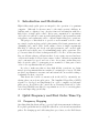
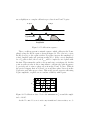
The amplitude can be tuned up by just sweeping the Gaussian amplitude
from zero for a fixed length in time as shown in figure 1, until a maximum
in the probability of the |1i state is achieved. This will serve our purposes
for now, as we just need large, but not necessarily perfect excitation of the
qubit.
1
http://www.physics.ucsb.edu/ martinisgroup/theses/Ansmann2009.pdf
4
456')%0)"789,/($&)
!"#$%&'%($')
*"+,$-./%0
1)%0$')"23
Figure 1: First Order π-Pulse tune up sequence.
2.3
Ramsey Fringe
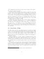
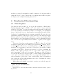
The Ramsey fringe experiment is a very sensitive way of checking how well
the qubit frequency is being tracked. The sequence, as shown in figure 2, is
an Xπ/2 -pulse followed by some delay and ending with a second π2 -pulse with
the microwave phase θ swept from 0 − 2π. Since we do not have finely tuned
π
-pulses yet, we may just use our first order π-pulse with the amplitude
2
halved.
!"123
45))6"7),%8
"9"123
!"#$%&'%($')
*"+,$-./%0
:)%0$')";<
Figure 2: Ramsey fringe pulse sequence
As a baseline, we set the delay such that the pulses are well separated,
and then sweep the phase of the second pulse to get a curve that should
resemble P1 = cos θ. Note that there are some phase errors in our π2 -pulse, as
the |1i state probability P1 is not always maximum at θ = 0 and minimum
at θ = π. However, we are not interested in these types of errors for this
experiment. We will correct them later, as described in section 3.3.2 on page
15.
We are most interested in observing how these maxima and minima (or
”fringes”) change with delay between pulses. If we are exactly on resonance
with the qubit frequency, these should be completely insensitive to the delay.
5
However, in reality we set our microwave signal to track the qubit frequency
to ensure the correct phase on applied microwaves. If there is some error
in frequency, we will see it manifest as the values of θ for the maxima and
minima in P1 change as a function of delay.2 So, by sweeping the delay and
θ we can map out just how accurately we are tracking the qubit frequency.
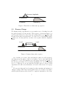
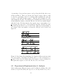
At this point it is likely that we see some drift in the maxima and minima
of P1 , as shown in figure 3. Using this experiment, it is easy to observe even
a few MHz frequency error, for even an error of this size will be substantial
when accrued through a typical qubit lifetime of T1 = 500 ns. An error of
a mere 5 MHz can give a 90◦ phase error in just 100 ns, turning an X-pulse
into a Y-pulse.
2.4
Tracking the Qubit Frequency Precisely
Now that we have a method for measuring small frequency errors, we must
correct them. Although we could use the Ramsey fringe as outlined in the
previous section as a way of correcting for these errors, there is a simple
and easily scriptable solution that does not require a 2-D sweep. Using the
following technique will allow us to lower frequency tracking errors to the
10−5 range.
The frequency calibration experiment is a slightly modified Ramsey fringe.
However, it is only a 1-D sweep so the calibration time is much faster. The
pulse sequence is a X π2 -pulse followed by a second X π2 -pulse with the delay
between them swept. However, the second pulse is tracking a frame processing at a slightly different frequency than the qubit.3 This is equivalent to the
axis of rotation for the second pulse to be rotating at a speed of the detuning
with respect to the actual qubit frame. We choose 50 MHz as it provides
well enough separated oscillations that allow us to determine the correction
needed but is fast enough to avoid large decoherence errors.
When we measure P1 , we find that it oscillates at a frequency of around
50 MHz. Any deviation from the 50 MHz tells us exactly how far we are from
the qubit frequency. We then adjust the microwave drive frequency until we
2
Note how the phase errors mentioned previously are unimportant because we are only
interested in the relative change in θ as a function of delay, not the absolute values of θ
for the maxima and minima.
3
It is important to note that the second pulse is on resonance with the qubit; only the
frame tracking that affects the phase of the pulse is detuned.
6
190
0.72
170
0.64
150
0.56
110
0.48
P1
Delay [ns]
130
90
0.40
70
0.32
50
30
10
-0.25
0.24
0.0
0.25
0.5
0.75
1.0
1.25
1.5
1.75
0.16
Phase/pi of second pulse
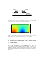
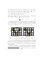
Figure 3: Ramsey Fringe - 10 MHz detuned. Note that the fringes are not
constant in the vertical (delay) axis. This tells us that the fringes are not
insensitive to delay, implying the microwave drive is not on resonance with
the qubit frequency.
200
0.72
160
0.64
0.48
80
P1
Delay [ns]
0.56
120
0.40
0.32
40
0.24
0.16
-0.25
0.25
0.75
1.25
1.75
Phase/pi of second pulse
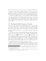
Figure 4: Ramsey Fringe - 2 MHz detuned. Again, we notice the fringes
shifting with delay. Notice how sensitive this experiment is for even a 2 MHz
detuning.
measure 50MHz oscillations as precisely as we can measure it.4
As a final check, shown in figure 6, we may perform a 2-D Ramsey fringe
to confirm that we are sufficiently on resonance. Once we are confident in
our measurement of f01 , we can use a similar technique to calibrate f12 by
adding in a π-pulse to go from the |0i to the |1i state, and then perform the
4
Note that this process is easily scriptable.
7
!"#$%
&'(()"*(+,-
"."/0123
!"95,:6,;56(
<"=+5>?@,4
1(,456("78
Figure 5: Frequency tuner pulse sequence
tune up procedure for the |1i − |2i transition as described previously. With
both f01 and f12 we can easily calculate the nonlinearity ∆.
190
0.72
170
0.64
150
0.56
110
0.48
P1
Delay [ns]
130
90
0.40
70
0.32
50
30
10
-0.25
0.24
0.0
0.25
0.5
0.75
1.0
1.25
1.5
1.75
0.16
Phase/pi of second pulse
Figure 6: Ramsey Fringe - On Resonance. We see that the fringes locations
are insensitive to the delay, showing us that we are on resonance.
3
3.1
Microwave Calibration: X & Y Quadrature
Phase Errors
As we can see from figure 7, we notice that our initial calibration does not
give a P1 with a maximum at θ = 0 and minimum at θ = π. This is due
to some phase error from our π2 -pulses. Due to the nature of our design, the
qubit is not a perfectly ideal two level system. The presence of the |2i state
enables unwanted virtual transitions during qubit gates which results in a
phase error.
8
1.0
0.8
P1
0.6
0.4
0.2
0.0
0.5
0.0
0.5
1.0
1.5
2.0
Phase/pi of second pulse
Figure 7: Ramsey Fringe - Phase Error
Given parameters for a fast gate, we find these phase errors to be around
5 - 10◦ . This is a significant error, but also problematic because it is just
large enough to cause substantial problems in long sequences, but small
enough that it can be difficult to measure directly.
◦
3.2
Amplified Phase Errors (APE)
We seek some method that will amplify this error in such a way that we can
better measure it. In order to do this, we must investigate the nature of
these errors and how they affect the gates.
3.2.1
Phase Error Analysis
We may model these errors in a simple way. Consider an ideal Xπ/2 -pulse
given by the transformation
1
1 −i
= e−iσx π/4 .
(1)
Xideal = √
−i
1
2
However, we find from experiment and simulations that a physical gate
is modified in the following way:
0 e−i
1
−ie−i
Xphysical = √
.
(2)
−i
e−2i
2 −ie
9
Xphysical = e
−i0
Z Xideal Z ,
Z =
1 0
,
0 e−i
(0 < 1),
(3)
where Z is the phase error generated from virtual transitions to the |2i state.
For the time being, we will ignore the global phase error 0 as we are only
concerned with single qubit gates.5
In the spirit of metrology, we look to construct a type of operation that
will amplify and measure this phase error without otherwise changing the
state of the qubit. Consider two types of simple gate identities, one which
consists of a net 2π rotation by stringing together 4 π2 -pulses, and one which
is a positive, then negative θ rotation. As is calculable from the error model
4
in equation 3, Xphysical
= −e−4i I; the 4 π2 pulses end up canceling out the
phase error that we are interested in. For this reason, we will explore the
general θ rotation identity more explicitly. Consider a general θ rotation
−i sin 2θ
cos 2θ
.
(4)
Xθ =
cos 2θ
−i sin 2θ
Now, consider an identity using this transformation by concatenating a
positive then negative6 θ rotation. For a first order expansion with 1 we
find
Iθ =
Z Xθ† Z2 Xθ Z
i(cos θ − 1)
sin θ
≈I+
(θ) + O(2 ).
− sin θ
−i(cos θ + 3)
(5)
This result is complex, as is a function of θ. From simulation, we
calculate (θ), shown in figure 8. We notice that increases monotonically
up to θ = π. However, given the form of Iθ , we find that Iπ = e−2i I; the
relative error that we are interested in cancels out no matter the value
of as noted above. We accumulate a global phase error, but we are not
interested in this at this time.
5
It is important to note that global phase errors will become very important for multiple
qubit experiments, however we seek a method of calibrating out these kinds of errors with
only a single qubit. Fortunately, the method we develop seems to correct for global phase
errors as well.
6
Theoretically it is perfectly equivalent to do a negative, then positive θ rotation.
However, as described in section 3.2.2 it is experimentally desirable to do the opposite.
10
0.45
0.40
Epsilon [radians/pi]
0.35
0.30
0.25
0.20
0.15
0.10
0.05
0.00
1.0
0.5
0.0
0.5
1.0
Theta [radians/pi]
Figure 8: Phase Error
To investigate the ideal value of θ, consider a state that is sensitive to
phase. We investigate Iθ acting on that state and consider only the relative
phase error ∆φ, defined by
1
1
1
1
7
8
|ψi = √
,
Iθ |ψi ≈ √
(6)
−i∆φ .
−i
−ie
2
2
∆φ is an experimentally significant value, as it is generated from and
is physically present in the qubit state. We can plot the relative phase error ∆φ(θ) from simulation which combines (θ) from figure 8 and Iθ from
equation 5, shown in figure 9.
Although the maximum is at θ ≈ 0.65, for experimental convenience
we restrict ourselves to a π2 -pulse. We sacrifice roughly 20% of phase error
generation, but ensure that we are using well defined and calibrated pulses.
For θ = π2 , we find
−i
Iπ/2 = I +
+ O(2 ).
(7)
− −3i
Using the Iπ/2 operation we can generate ∆φ = 2 phase error. We must
now develop an experiment that allows us to use this operation to generate
a phase error that we can measure.
7
8
It is important to note that |ψi must be located on the Y or -Y axis, as Iθ rotates about the X axis.
Again, we neglect global phase.
11
Relative phase error phi [radians/pi]
0.07
0.06
0.05
0.04
0.03
0.02
0.01
0.00
0.0
0.2
0.4
0.6
0.8
1.0
Theta [radians/pi]
Figure 9: ∆φ Phase Error
3.2.2
Experimental Implementation
As we saw in figure 7, a Ramsey fringe is sensitive to the phase error. Now
that we have an operation that will amplify this error, we can insert one or
multiple Iπ/2 operations in order to amplify the phase error. This is the
Amplified Phase Error (APE) sequence shown in figure 10.
&'()*+,+-&""'#$%
!"#$%
"."#$%
!"620(30+23)
/)0123)"45
7"892:;,01
Figure 10: Amplifying Phase Error (APE) sequence
As is seen through matrix algebra in equation 8, each Iπ/2 identity acting
on an equator state prepared by a Xπ/2 -pulse adds an extra ∆φ = 2 phase
error. Repeating this Iπ/2 operation will add more phase error and increase
the size of this effect.
1
|ψi = √
2
1
,
−i
1
Iπ/2 |ψi = √
2
e−2i
1 − 2i
1
≈ √
−2i
−i − 4
2 −ie
(8)
Experimentally, we find that we can insert 5 identities before phenomena
12
such as T1 , T2 and the nonlinearity of the phase error give us adverse effects.
This allows us to magnify the phase error by roughly an order of magnitude, where we measure almost 90◦ of phase error as in figure 11. From the
experiment, we find that is important to do a positive then negative θ rotation for the identity operation to have the Bloch vector “bouncing” against
the |1i state rather than |0i. It seems that doing so minimizes resetting of
the qubit due to T1 relaxation and destroying phase error that we are trying
to accumulate.
1.0
0 operations
1 operation
2 operations
0.8
3 operations
4 operations
5 operations
P1
0.6
0.4
0.2
0.0
0.5
0.0
0.5
1.0
1.5
2.0
Phase/pi of second pulse
Figure 11: APE - Uncorrected phase erorr accumulation.
3.3
3.3.1
Phase Error Correction
Derivative Removal by Adiabatic Gate (DRAG)
A technique known as Derivative Removal by Adiabatic Gate (DRAG)9 has
been developed by F. Motzoi et al. as a method of combating previously described gate errors. When performing a gate operation about the X quadrature, the Y and Z fluxbias remain idle. DRAG provides a way of using these
idle degrees of freedom in order to dynamically detune the microwaves and
qubit in a way that compensates for both the actual and virtual occupation
9
Phys. Rev. Lett. 103, 110501 (2009)
13
of the |2i state, preventing amplitude and phase errors. According to DRAG
theory, one sets:
(λ2 − 4)Ex2
Ėx
and
δ1 =
(9)
∆
4∆
where Ey is the Y quadrature of microwaves,
√ δ1 is the qubit detuning, ∆ =
2π(f12 − f01 ) is the nonlinearity and λ = 2 describes the relative strength
between the 0-1 and 1-2 transitions. However, this triple control can be
challenging as it requires using a separate Z fluxbias control in conjunction
with both X and Y with precise timing and amplitude. In addition, generally
these Z contributions are small and errors can arise from DAC discretization.
However, it turns out that there is a convenient way of sidestepping this
problem.
Ey = −
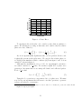
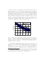
Figure 12: DRAG - Gate fidelity for combinations of Y and Z contributions.
A value of 1.0 corresponds to the original theoretical value.
As is seen in the simulated data from figure 12, if we add coefficients to
the δ1 and Ey contributions and modulate them, we find that they are both
contributing similar effects to gate fidelity10 . Rather than try to coordinate
10
Gate fidelity is calculated as F = tr(χsimulation χideal ), where χ is calculated from
quantum process tomography. See section 4.
14
two contributions at the same time, we can simply set δ1 to 0 and calibrate
the Ey coefficient for an optimal value, which we find to be 12 . Doing so
removes the Z-control and any associated calibration issues.
3.3.2
Half Derivative (HD) Method
Half Derivative (HD) method is based on the control theory of DRAG. It is
named after the coefficient of 21 on the Ey term, is given by:
Ėx
and
δ1 = 0
(10)
2∆
For a single qubit in ideal circumstances such that Ex /∆ is small, HD can
be directly applied and does not require any tuning.11 As is visible in figure
13, we can see that HD corrects for large amounts of the phase error, keeping
the maxima and minima of P1 close to θ = 0 and θ = 1 respectively.
Ey = −
1.0
1.0
0 operations
1 operation
2 operations
0.8
0.8
3 operations
4 operations
5 operations
P1
0.6
P1
0.6
0.4
0.4
0.2
0.2
0.0
0.5
0.0
0.5
1.0
1.5
2.0
Phase/pi of second pulse
0.0
0.5
0.0
0.5
1.0
1.5
2.0
Phase/pi of second pulse
Figure 13: APE - Single-quadrature Gaussian (left) and HD (right).
To get a more intuitive picture as to just how HD improves the qubit
gates, we can use state tomography to map out the gate trajectory along the
Bloch sphere. We increase the amplitude of a pulse from 0 to π, and perform
state tomography at each amplitude step. We then map the state back onto
the Bloch sphere.
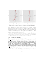
As can be seen in figure 14, a one quadrature Gaussian suffers amplitude
and phase errors as the trajectory drifts away from the pole of the Bloch
11
The amplitude may need to be re-calibrated for HD pulses as it can differ slightly,
around 1%, from a single-quadrature Gaussian.
15
Figure 14: Bloch Sphere Trajectory - Gaussian (left) and HD (right)
sphere. This effect is dramatic using tomography, but P1 masks just how
significant of an error this as at the pole of the Bloch sphere since P1 is first
order insensitive to phase errors. In the HD pulse, the trajectory is directly
down the meridian and appears to have greatly reduced phase error. HD is
the ideal computational pulse that we seek.
To alleviate any last concern that we may have about this HD technique
for improving microwave pulses, we may use quantum process tomography
to compute a χ matrix and overall gate fidelity, as in figure 18.
3.3.3
Caveats and Tunability
When deriving the math behind DRAG and HD, an assumption is made
that E∆x 1 in order to perform a taylor expansion. However, even in the
most ideal cases when operating a phase qubit, this is not necessarily the
case. When using shorter pulses such as a full width half maximum time of
5 ns, and with a relatively large ∆ = 2π(200 MHz), we find E∆x ≈ 12 , which
is hardly a small parameter. The basic mathematics still hold fairly well
even in these extreme circumstances, but with a smaller nonlinearity (such
∆
as 2π
= 100 MHz) the expansion breaks down. In this case, HD can still
dramatically improve qubit gates.
Rather than worry about the HD protocol in this limit, we can take the
16
basic idea and simply tune the correction for best performance. We insert a
coefficient α in front of the Y quadrature component and tune this parameter
to an optimal value. Under normal circumstances, α = 12 , but in less ideal
limits, we can use the APE sequence to tune α in a way that minimizes phase
error.
In summary, we can use the following protocol for HD in the limit of short
pulses or small nonlinearities:
Ėx
and
δ1 = 0
(11)
∆
Where α is tuned to remove phase error on the APE sequence. We find a
value typically within 20% of 21 . There are two types of dominant errors;
|2i state errors which are minimized by Gaussian pulses, and phase errors
that which can be removed by tuning α. Thus we can easily maximize gate
fidelity with these methods.
Ey = −α
4
4.1
Quantum Process Tomography
Formalism
Methods such as APE only probe specific aspects of our microwave control,
such as phase errors. In order to get a complete picture of our gates we can
use Quantum Process Tomography (QPT). This mathematical framework
can be used to completely describe the transformation independent of the
input state.
The methodology for describing a qubit gate is as follows. We wish to
describe the transformation in a complete and general way by inserting some
initial state ρ and the transformation returns some different state E(ρ).
X
E(ρ) =
Em ρEn† χmn
(12)
mn
Where {E} form a basis for the set of operations on ρ. The χmn scalars
weigh each individual process labeled by m, n. The χ-matrix itself therefore
completely describes the process in some basis of {E}. This kind of formalism
is essential as decoherence errors prevent the transformation from being truly
17
unitary. Consult Quantum Computation and Quantum Information 12 for
more detail.
4.2
Experimentally Constructing χ
State
Perparation
Quantum
Process
State
Tomography
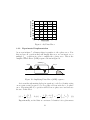
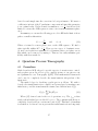
Figure 15: Quantum Process Tomography
The next step is experimentally determining what the χ-matrix for a
qubit gate and compare it to the ideal, an overview of the experimental
procedure is given in figure 15. This can be done by initializing the qubit
in various input states that span the space of possible states, transforming
the state with a qubit gate, and performing tomography such as in figure 16
to reconstruct the state afterwards. By using tomography on the initial set
of basis states and the states after the transformation, we can reconstruct
what the transformation does independent of input state by computing the χmatrix by the process shown in figure 17. For further detail on experimental
process tomography, see M. Neeley et al. Nature Physics 4, 523-526 (2008).
Initial state
ρi
Set of Basis
Rotations
Measure
Reconstruct
state ρi
Figure 16: State Tomography - The set of basis rotations rotate the state
such that each measurement will be equivalent to projecting the state on
orthogonal axes.
Once we have obtained a χ-matrix, we may compute the operation fidelity
defined as F = tr(χexperiment χideal ). We may also view the matrix to get
specific error information; the χ-matrix tells us all the desired and undesired
operations that occur in the transformation. Figure 18 shows experimental
data for both HD and single-quadrature Gaussian π-pulses.
12
Nielsen, M.A. & Chuang, I.L.. Quantum Computation and Quantum Information
(Cambridge Univ. Press, Cambridge, 2000).
18
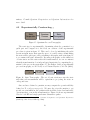
Prepare
states {ρi}
Result
states {ρf}
Quantum
Process
Reconstruct
{ρi} , {ρf}
State
Tomography
Use {ρi} , {ρf} to calculate χ
Figure 17: Calculating χ
I
σx
σy
σx
σz
σy
σz
I
I
σx
σy
σx
σz
σy
σz
I
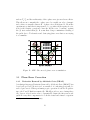
Figure 18: Quantum Process Tomography - Real part of the χ-matrix for
single-quadrature Gaussian (left) and HD (right) in the Pauli {I, σx , σy , σz }
basis. The only ideal matrix component is the σx , σx component. Notice
how HD corrects for the σz , σx error process. Imaginary components of the
χ-matrix not shown as error elements are small and not strongly effected by
HD.
5
Flux Bias Calibration: Z control
Up through this point, we have high fidelity control for any X or Y gate,
as well as any combination of the two. However, what has gone completely
untouched is Z control. Fortunately, once the microwaves are tuned up this
becomes relatively straightforward. The Z control works by changing the relative phase between the |0i and |1i state, but does not excite any transitions
between them. The challenge in tuning up Z gates is that to read out the
qubit we measure P1 . Since Z gates do no directly effect this value, we must
19
use a slightly more complex calibration procedure from X and Y gates.
+",-.
"9",-.
+">%)82)7%23
=">%)82)7%23
/0123)*3
"456$(7%83
!"#$%&'()*
:3)*%23";<
Figure 19: Z calibration sequence
These conditions present a natural sequence which calibrates the Z amplitude along the Bloch equator, shown in figure 19. The idea is to rotate
the Bloch vector to the equator with a Xπ/2 -pulse, increase the amplitude of
a fixed length Z pulse and perform another Xπ/2 . If the correct amplitude
for a Zπ pulse is used, the second Xπ/2 will be completely out of phase with
the first. This returns the qubit to the ground state, as in figure 20. At this
point we will note why it was so important to calibrate the qubit frequency
so precisely and to remove phase errors from the X and Y gates. Without
the precise bring-up that we followed, we would have phase errors from the
X gates in our Z tune up procedure. This would give us errors in calibrating
Z gate amplitude, as phase errors combine additively with Z gates.
0.8
P1
0.6
0.4
0.2
0.0
0.10
0.05
0.00
Z amplitude [a.u.]
0.05
0.10
Figure 20: Z calibration data - Notice the minimum in P1 around the amplitude of 0.035.
As the Z control does not excite any transitions between states, we do
20
not have to worry about virtual or actual occupation of a 3rd state such as
during the X and Y gates. This is why no technique such as HD is required
for Z gates, and a simple Gaussian pulse will do.
6
6.1
Randomized Benchmarking
Pulse Sequence
Now that the qubit is tuned up, we can use the technique of Randomized
Benchmarking developed by Knill et al.13 and carried on superconducting
qubits by J. M. Chow14 as a way of getting an averaged measure of qubit gate
error. The technique essentially is a method of averaging over all different
types of qubit gates to get a single number representing the qubit fidelity.
As this is a benchmarking that is averaging essentially all errors, it is not
particularly useful as a tune up procedure, but it is a nice final check after
all tune up has been performed to qantify how a device is performing. This
has advantages over tomography as it averages over all computational gates
and does not scale exponentially with the number of qubits, as tomography
does.
Q
The protocol involves a pulse sequence Rf i Ci Pi , where Pi are Pauli
rotations (π-pulses) and Ci are Clifford group generators ( π2 -pulses), and Rf
is a final π2 -pulse. The idea is to randomly generate a series of uncorrelated,
interleaved π and π2 -pulses of any axis or direction to test all the potential
operations of the qubit. However, we want to be able to determine the
fidelity of all of these operations, and we do not want to have to perform
state tomography15 at the end of a sequence. The purpose of the Rf pulse is
to rotate the Bloch vector onto the Z axis16 so that a simple P1 measurement
can be used to determine fidelity. Then, we can perform multiple tests of
various lengths to get an idea of how overall fidelity drops over numerous
gate operations, and use this information in order to determine the average
error associated with each gate.
Rather than randomizing every single operation, we take the approach
13
Phys. Rev. A 77, 012307 (2008)
Phys. Rev. Lett. 102, 090502 (2009)
15
See section 4.2.
16
If the Bloch vector is already aligned with the measurement axis, an identity operation
is performed.
14
21
of generating a long random sequence, and probing the fidelity after every
iteration within it. First, we generate the longest sequence that we wish
to check by generating a list of of variables that determine the axis and
rotation of each pulse in that sequence. This list will determine all of the
pulses minus the Rf pulse. The challenge is determining the fidelity at various
points within the sequence, when the Bloch vector is not necessarily aligned
with the Z axis. We then truncate the sequence up to some number of π,
π
iterations and tack on the corresponding theoretically calculated Rf pulse
2
that will bring the Bloch vector to the Z axis. This gives us the fidelity of
the sequence after some number of iterations. This process is described in
figure 21.
!"
#
$
%
&'()*(+,-(*./
0+-'1,+)2&
!"
#
$
%
&'()*(+,-(*./ 3/4)*(+,-(*./
0+-'1,+)2&
!"
#
$
%
&'()*(+,-(*./ 3/4)*(+,-(*./ 5,4)*(+,-(*./
0+-'1,+)2&
Figure 21: Randomized Benchmarking - Probing the fidelity as various points
in a long sequence. Measuring the fidelity after 1, 2, and 3 iterations of π,
π
-pulses. Notice how Rf changes after each sequence, as it is calculated by
2
each particular sequence to move the Bloch vector to the Z axis.
6.2
Experimental Implementation & Analysis
After testing many different sequences and checking the fidelity after each
iteration, we plot the fidelity and expect to see an exponential decay due to
22
decoherence and gate error accumulation. We know that at zero iterations,
the fidelity should be at 1.17 We also expect that after many iterations, the
fidelity should reside around 0.5. Given these assumptions, we may simply fit
the parameter b in the exponential F = 0.5e−bni + 0.5. This functional form
gives us the exponential behavior we seek as well as the boundary conditions
that we stipulate. The variable b then can be interpreted as the “error per
iteration”. As each iteration has 2 gates, b/2 gives us an average “error
per gate” that we wish to quantify. Figure 22 shows experimental data for
randomized benchmarking, as well as the exponential fit.
1.0
Benchmarking Data
Exponential Fit
Sequence Fidelity
0.9
0.8
0.7
0.6
0.5
0.40
5
15
10
20
Number of 2-gate iterations n
25
30
i
Figure 22: Randomized Benchmarking - Experimental data for 40 different
sequences. Variance in fidelity is consistent with statistics for 600 experiments per data point. Gates are 5 ns full width half maximum with 7 ns
between the center of each gate.
Notice that the exponential fit in figure 22 does not go exactly to 1 as
iterations goes to 0. This data set was least-squares fit to a two parameter
function: F = Ce−bniterations + 0.5. This is a way to double check that our
measurement correction is behaving as we expect. For this experiment, we
find that C = 0.490 and b = 0.0494. This value of C within 2% to the ideal
17
This assumes no measurement error. In this case, we have corrected for measurement
error to validate this assumption. For more on measurement error correction, see the
supplemental information of R.C. Bialczak et al. arXiv:0910.1118v1
23
value of 0.5 is consistent with accurate measurement error correction. The
value of b corresponds to an experimental “error per gate” of 2.47%, where
we consider each iteration in the protocol as 2 gates.
7
Gate Timing
Now that we have carefully tuned microwave gates and have a standard
for computing gate and sequence fidelity in an precise way, we can begin
to consider more complicated multi-gate experiments. Previously, we were
trying to extract useful information out of experiments. During tune up
procedures, it is important to keep qubit gates well separated as we want
to avoid overlap errors at the cost of suffering more greatly from predictable
errors such as T1 and T2 . As we move forward, we can begin to consider how
optimize for every last bit of fidelity out of our qubits.
Currently, the greatest source of error in any quantum algorithm comes
from decoherence. With this in mind, each experiment is some what of a
“race against time”, where we try to accomplish as much as we can before
decoherence destroys all information in the qubit. To combat this, we can
push our gate operations closer together and make individual gates shorter.
However, it is important to strike a balance between overlaping gates and
decoherence, as either can generate substantial errors. Given that a Gaussian
has infinite extent unless we truncate it, the question becomes just how close
together do we place them?
By varying the gate delay in randomized benchmarking, we notice that
there is a point where gates are spaced too closely together as the fidelity
of certain sequences plummets, quickly dragging down the average error per
gate, as seen in figure 23. Randomized benchmarking is not a tune up procedure per se, but it can be useful in finding correct gate spacing in general as
it provides a “global” approach to testing virtually every kind of sequences
for a set of parameters.
Process tomography provides us a metric for optimizing individual sequences, and again can provide a method for optimizing gate delay, in a
similar vein to randomized benchmarking.
Although these methods are not particularly elegant, they provide a precise way of combating a complicated problem.
24
1.0
Benchmarking Data
Exponential Fit
0.9
Sequence Fidelity
0.8
0.7
0.6
0.5
0.4
0.30
5
15
10
20
Number of 2-gate iterations n
25
30
i
Figure 23: Randomized Benchmarking - Overlap errors greatly reduce fidelity
of some sequences, as seen by the overall drop in fidelity and increase in
variance. In this data, gate delay is 6 ns as opposed to 7 ns previously. All
other parameters are identical to figure 22. An overall drop in “error per
gate” is seen as b = 0.0562.
8
Conclusions & Moving Forward
In the process of bringing up and calibrating a qubit, we find bootstrapping to be an essential aspect in the procedure. We are able to discover
and optimize fundamental aspects of a qubit via clever experimentation and
careful analysis. In addition, we have built on previous work by developing
the APE sequence to better measure phase errors, and implemented DRAG
in an experimentally convenient way in order to correct for them.
At this point we have a tuned up single qubit for all relevant computational gates. Through process tomography and randomized benchmarking we
also have a good idea how each gate is working. Although everything should
be working preceisely at this point, we have several tools for inevitable troubleshooting that will be required in performing an experiment.
25