Download Berkeley Water Center Data Cube

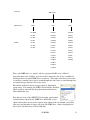
USA
USA
USA
USA
-
AK
ME
ME
MI
-
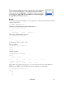
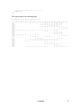
Atqasuk
Howland Forest (main tower)
Howland Forest (west tower)
Sylvania Wilderness Area
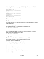
The actual air temperature data is in the array cube_query_out.data. If we wanted the
temperature for the Finland sites (columns 1-4) for the 30th of January (the 30th day of the
year--row 30), we could view them with:
>> cube_query_out.data(1:4,30)
ans =
-7.8342
-13.0844
NaN
-11.4312
This tells us (aside from our Finland sites being cold in January) that there is no data for
Siikaneva fen.
Plotting these data
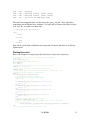
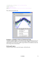
Here is an example of a script to plot the result data as a time-wise scatter plot.
% make sure we have access to our return data in the global
% data space
global cube_query_out;
% create the figure window with axes
fh = figure();
ah = axes();
% These will be the symbols we use for the various sites
symbols = '+ox*sd^Vph.';
% There's only 366 days, so set limits on the X axis
xlim([1 366]);
% iterate through the sites on the first dimension, choose colors and
% symbols, and plot each site's data series
hold on;
for i=1:cube_query_out.dim_sizes(1)
% choose the color for the country
% we will make an unknown country magenta
color = 'm';
if strfind(cube_query_out.axes{1}{i},'Finland') == 1
color = 'g';
end
if strfind(cube_query_out.axes{1}{i},'Russia') == 1
color = 'r';
end
if strfind(cube_query_out.axes{1}{i},'Sweden') == 1
color = 'k';
end
if strfind(cube_query_out.axes{1}{i},'USA') == 1
color = 'b';
end
% set up the color/symbol as the linespec
linespec = [symbols(i) color];
% plot the site temperatures, day numbers on the X axis, temperature
% data on the Y axis
plot(1:cube_query_out.dim_sizes(2),cube_query_out.data(i,:),linespec);
end
% Set up a legend using the Sites dimension axis
11/10/2008
21