Download Gravity corrections (T54)

INTREPID User Manual
Library | Help | Top
Gravity corrections (T54)
1
| Back |
Gravity corrections (T54)
Top
The INTREPID Gravity tool can apply gravity corrections and calculate gravity
anomalies for land gravity data, and also marine and airborne gravity data.
In this chapter:
•
Overview of the gravity corrections tool
•
Key concepts for Land Gravity Acquisition
•
Data reduction and network adjustment
•
Utility gravity transforms
•
Terrain correction
•
Gravity mode settings
•
Specifying input and output files
•
Process menu
•
Tools menu
•
Spatial query
•
Settings menu
•
View menu
•
Help
•
Using task specification files
•
Gravity processing reports
•
Frequently asked questions
For worked examples showing the use of the Gravity tool, refer to the Cookbook
Gravity field reduction and correction (C08)
Overview of the gravity corrections tool
Parent topic:
Gravity
corrections
(T54)
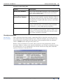
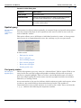
You can use the help menu to display help text on the topics shown in the menu
illustration below.
The INTREPID Gravity tool has four main functions:
Data reduction and network adjustment
Import land gravity field data in either AGSO or Scintrex format, and reduce the loop
data to final Observed Gravity, FreeAir and Bouguer anomalies. This is a complete
bundled processing sequence which involves several stages, including gravimeter
calibrations, data integrity and loop structure checks, Earth tide and gravimeter drift
corrections, network adjustment and global tie-in to gravity base stations. A principal
facts database is created from the reduced data.
Terrain correction
Using a Digital Elevation Model (DEM), calculate terrain corrections for either land,
marine or airborne data. The terrain correction can then be used to compute the
Complete Bouguer anomaly. Full tensor gravity terrain corrections are also
supported.
Moving Platform Gravity and Gradiometry Support
INTREPID has support for many instruments and systems for gathering gravity or
Library | Help | Top
© 2012 Intrepid Geophysics
| Back |
INTREPID User Manual
Library | Help | Top
Gravity corrections (T54)
2
| Back |
gradiometry from a craft that is moving. This covers the older L&R sea meters,
including a direct algorithmic link to the original LaCoste decorrelation of wave
action accelerations from the gravity. This came via a collaboration with Herb Valiant
of ZLS. Also supported is the inline & cross-line geometry matrix transforms for the
Lockhead-Martin Full tensor gravity gradiometry system. The FALCON instrument
is also fully supported, though some of the support is distributed through several
tools, especially the gfilt FFT tool, as some of the transforms have to be done using
Foyurier transforms using gridded data. The GTXX, Rio VKX and Sanders
instrumental systems have also been processed using this tool.
Utility gravity transforms
Open an existing gravity dataset and perform stand-alone gravity transforms, for
example, forward and reverse transformations of FreeAir and Bouguer anomalies, or
convert from one gravity Datum to another gravity Datum.
Key concepts for Land Gravity Acquisition
Parent topic:
Gravity
corrections
(T54)
You can use the help menu to display help text on the topics shown in the menu
illustration below.
Survey loop
For land gravity surveys, the basic data acquisition procedure is the loop. It is
required to remove the gravimeter’s drift during the data reduction process. The
INTREPID Gravity tool requires that loops must start and stop on the same station,
unless one is a control base station, in which case they are allowed to be different.
Survey network
A land gravity survey network is a series of interlocking closed loops of gravity
observations.
Gravimeter loop set (GMLS)
The GMLS is defined as one gravimeter-operator combination.The INTREPID
gravity tool allows for processing of large gravity datasets that could involve multiple
gravimeters and operators over many years.
Nodes
Nodes are gravity stations where more than one reading was observed.
Global nodes
Global nodes are gravity stations common to more than one gravimeter.
Gravity base stations
These are locations where the gravity value is well defined. One or more main gravity
base stations are used as a reference, or control, for local surveys. The Global
Adjustment processing stage ties all the GMLS survey stations back to these base
stations.
The nature of the Global adjustment depends upon the number of Control stations.
Where there is a single Control station, INTREPID holds that station fixed and
adjusts all other stations to it. However where there is more than one Control station,
INTREPID calculates a global adjustment by averaging the changes to each Control
station made as a result of the network processing. In this case no single Control
station remains fixed. It is presently not possible in INTREPID to influence the
relative weightings of the Control stations.
Library | Help | Top
© 2012 Intrepid Geophysics
| Back |
INTREPID User Manual
Library | Help | Top
Gravity corrections (T54)
3
| Back |
Data reduction and network adjustment
Parent topic:
Gravity
corrections
(T54)
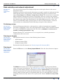
You can use the help menu to display help text on the topics shown in the menu
illustration below.
Field data reduction and network adjustment can only be applied to land gravity data
which has the survey loop structure clearly defined. The process consists of two
stages, Data Import and Reduce Loop data to Final. The intent here is to provide
high redundancy through good survey loop design, with one or more base stations,
master nodes for each loop, and repeat stations that may not be nodes. The design of
the software also makes the distinction for each Meter/Operator pair, as the care
taken by an individual with a gravity meter is also very characteristic. 3 levels of
error analysis are undertaken in the following 16 steps of data reduction.
Preliminary set-up
Parent topic:
Data reduction
and network
adjustment
For non-Scintrex gravimeters, each meter has a table of manufacturer supplied
gravimeter calibration values, also called instrument factors. These must be included
in a special INTREPID configuration file. The file is (INTREPID installation
folder)/config/gravimeter.cfg.
Scintrex meters use a scale factor of 1.0 as a special case, and the gravimeter
configuration file is not used.
Data import formats
Parent topic:
Data reduction
and network
adjustment
The field data must be in one of the following three formats.
•
AGSO format
•
Scintrex format (CG3)
•
Scintrex format (CG5)
For details of the file formats, see Gravity import file formats (R27).
Data import
Parent topic:
Data reduction
and network
adjustment
From the File menu, select Survey Import Wizard. Select the data format to import.
The Mode box requires you to choose appropriate settings for the gravity Datum,
units, and survey environment. See Gravity mode settings. The next section mostly
applies to land Surface gravity acquisition, so choose Land Surface. The field data
can also be presented in various pre-defined formats. One is the AGSO gravity field
format, which is future proof, by reqyuiring data to be in a flat ASCII file, and also
requiring all the necessary data to be in just one file. Choose AGSO Gravity Field
Data.
Library | Help | Top
© 2012 Intrepid Geophysics
| Back |
INTREPID User Manual
Library | Help | Top
Gravity corrections (T54)
4
| Back |
Process to loop data
Parent topic:
Data reduction
and network
adjustment
The following sequence of 8 processing steps are applied to the data:
1
Position Data Check
2
Control Data Check
3
Calibration Calculation
4
Loop Data Check
5
Locate Nodes (Loop Ties)
6
Locate Global Nodes
7
Repeat Nodes Check
8
Data Structure Integrity Check
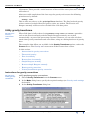
After the import process is finished INTREPID displays a report file to the screen. We
recommend you check the report carefully. In particular scroll to the bottom of the
report file and ensure that all 8 processing steps were applied to completion. Bad data
records, time reversals, excessive tares, duplicate loop numbers, can all cause the
processing sequence to stop prematurely. If this is the case you must go back to the
input data and resolve the problem before proceding further.
After successfully completing the data import, the gravity tool creates the following
point datasets:
Survey_ControlDB..DIR
This dataset contains the Control gravity station details.
Survey_LoopDB..DIR
This dataset contains the gravity survey data. The structure of this dataset reflects
the order of the aquisition loops.
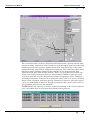
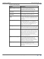
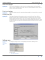
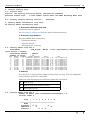
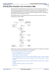
The gravity tool displays the field loop data that has just been imported.
INTREPID uses the following symbols to display the gravity dataset:
Gravity station (location of a gravity measurement)
Ties (nodes)—base station or station common to more than one loop
Repeated links between stations. Usually shown as white lines!
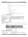
Click a station to view the data for that station. INTREPID displays the station data
in a message box.
Library | Help | Top
© 2012 Intrepid Geophysics
| Back |
INTREPID User Manual
Library | Help | Top
Gravity corrections (T54)
5
| Back |
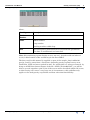
where:
Heading
Description
Station
Number
Station number
Index
GMLS number
Loop number
Reading number within loop
Dial
Raw field gravity measurement as read from the gravimeter.
The data is uncalibrated and unscaled.
Note: this numbering system begins at zero, not one! A station with an index of
(0,1,2) is third station of the second loop in the first GMLS.
The data used in this manual is supplied as part of the sample_data/cookbooks/
gravity_land. It comes from a Geoscience Australia gravity regional survey near
Goulbourn, NSW and was acquired in 1997. So, whilst this is a reference manual, by
doing an AGSO data format import of the file “AGSO_Week1&2.DAT”, you will be
able to see and reproduce quite a few of the screen states described within. Of course,
as this Gravity tool covers a very large set of circumstances, this guideline only
applies to the land gravity acquisition and data reduction functionality.
Library | Help | Top
© 2012 Intrepid Geophysics
| Back |
INTREPID User Manual
Library | Help | Top
Gravity corrections (T54)
6
| Back |
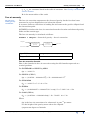
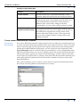
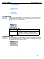
Click a station to
view the gravity
values
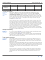
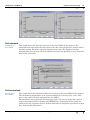
The convention above is that a single black dot represents a gravity station with
just one reading. Left mouse click a station to view the station data, including loop
number, loop set and sequence number in the loop. The dial value is the actual
number from the meter before calibration corrections. The white lines show nodes
that have many readings connecting key stations in the loop network. This
regional layout may seem foreign to some. There is a great diversity in how you
design successful gravity loop surveys, with Scintrex tending to push the “grid”
view more with the way the default meter wants to organise records. Temporal
and spatial coherence of the gravity readings are vital, if one is to create a reduced
dataset that accurately measures gravity anomalies in an area. All survey styles
can be accommodated in this tool, though sometimes it does seem to be a trial, if
your planning was not well documented!
INTREPID has the capacity to retrieve duplicate readings at the same station as
well - the station data in a message box.(Turned off at present)
Library | Help | Top
© 2012 Intrepid Geophysics
| Back |
INTREPID User Manual
Library | Help | Top
Gravity corrections (T54)
7
| Back |
Note: There is actually only one observed gravity record for each station in the
reduced dataset. The observed gravity for this station is the average of the displayed
values. See INTREPID gravity point datasets (R28) for details of the gravity point
dataset.
The station data records shown are from the imported loop data, where
Heading
Description
Station Number
Station number
Index
GMLS number
Loop number
Reading number within loop
Dial
Raw field gravity measurement as read from the
gravimeter. The data is now calibrated and scaled.
Gravity
Corrected observed gravity field. (For stations with
multiple reading contains the average only.)
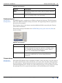
Stage 2 Data Reduction of Loop Data
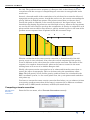
The next step is to apply another 8 steps, including loop levelling, to produce a
principal facts dataset from the field data. There is also a tie-in to one or more
absolute base stations, using a least squares drift algorithm, to estiamte the observed
value, Free Air and a Bouguer, together with an error estimate where more than one
occupation of a gravity station was undertaken. The overall accuracy of the survey is
also estimated. Follow the wizard prompts. You come to the point where the initial
Loop Database is requested below. Choose Finish..
Library | Help | Top
© 2012 Intrepid Geophysics
| Back |
INTREPID User Manual
Library | Help | Top
Gravity corrections (T54)
8
| Back |
Reduce loop data to final data
Parent topic:
Data reduction
and network
adjustment
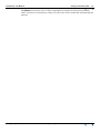
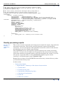
After the Data Import phase, you can reduce the loop data to final data. From the
Process menu, select Reduce Loop data to final. INTREPID asks you for another
Mode review and for output dataset names. The following sequence of processing
steps are then applied to the data:
•
Meter Correction (uses the gravimeter calibration file)
•
Earth Tide Correction
•
Meter Drift Correction
•
Node Levelling (network adjustment)
•
Global Adjustment of Loopsets
•
Apply Meter Scale Factor
•
Global Adjustment (tie-in to Control)
•
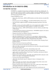
Report Final Values
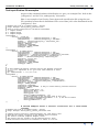
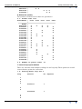
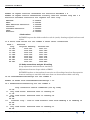
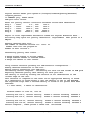
16: Final Values
Simple Bouguer Anomaly
Terrain type: land
Density: 2.670
Gravity datum: IGSN71_AGSO
Station
83910104
97050001
97053000
97051001
97051002
97051003
97051004
97051005
97051006
97051007
97051008
97051009
97051010
Latitude
Longitude
Observed StdDev
-35.29180 149.13793 979603.310 0.0000 44
-34.98653 149.02575 979573.630 0.3017 23
-34.92311 149.13862 979579.171 0.2667
7
-34.91766 149.17099 979579.775
1
-34.93752 149.20110 979582.801
1
-34.97068 149.22058 979581.946
1
-34.99010 149.26379 979584.837
1
-34.99623 149.22436 979582.031
1
-34.97846 149.18874 979567.771
1
-34.99529 149.16110 979564.220
1
-34.94436 149.15306 979572.780
1
-34.88974 149.13475 979560.296
1
-34.85413 149.13500 979566.550
1
No.
Height
565.000
613.030
551.991
556.609
559.904
576.656
579.199
586.229
638.322
654.965
589.025
645.721
604.947
Vert_Offset
Free Air
Bouguer
565.00
9.7995
-53.4221
613.03
20.9889
-47.6071
551.99
13.0920
-48.6739
556.61
15.5854
-46.6973
559.90
17.9376
-44.7138
576.66
19.4305
-45.0953
579.20
21.4519
-43.3585
586.23
20.2932
-45.3038
638.32
23.6218
-47.8043
654.97
23.7743
-49.5140
589.02
16.3217
-49.5882
645.72
25.9815
-46.2725
604.95
22.6806
-45.0110
After the Reduce Loop data process is finished INTREPID displays the appended
report file on the screen. Again we recommend that you check the report thoroughly.
Sections 11 and 12 contains precision statistics computed after drift, and after loop
Library | Help | Top
© 2012 Intrepid Geophysics
| Back |
INTREPID User Manual
Library | Help | Top
Gravity corrections (T54)
9
| Back |
adjustment. These provide a useful measure of how well the survey data was collected
and reduced.
After successful completion of the last step, the gravity tool creates the following
point dataset by default:
Survey..DIR
This is what we refer to as the principal facts database. The final reduced gravity
values consist of a single Observed gravity value per station. The Freeair and
Bouguer anomaly values are also calculated for each data point.
Utility gravity transforms
Parent topic:
Gravity
corrections
(T54)
When field data is fully reduced using Reduce Loop Data to Final, quantities
such as the Freeair anomaly and the Simple Bouguer anomaly are created
automatically, as part of the processing sequence. However you can also calculate
stand-alone gravity transforms and corrections, using an existing database of gravity
data.
The examples that follow are available in the Gravity Transforms options, under the
Process menu. The Gravity tool creates new fields to store these values.
In this section:
•
Instructions for gravity corrections
•
Theoretical gravity
•
Free air anomaly
•
Reverse free air anomaly
•
Simple Bouguer anomaly
•
Reverse simple Bouguer anomaly
•
Eötvös gravity correction
•
Velocity from Eötvös gravity correction
Instructions for gravity corrections
Parent topic:
Utility gravity
transforms
Library | Help | Top
>> To perform gravity corrections:
1
Choose Gravity Transforms from the Process menu.
2
In the Mode dialog boxes, specify the required settings (see Gravity mode settings
for details).
3
In the Gravity Transforms dialog box:
© 2012 Intrepid Geophysics
| Back |
INTREPID User Manual
Library | Help | Top
Gravity corrections (T54)
10
| Back |
Specify the gravity dataset for correction.
Select the correction that you require.
Choose Finish.
4
INTREPID asks you for the required input and output fields (see below for
details). INTREPID does not ask for a field name if there is a corresponding valid
alias.
5
INTREPID displays the current settings (if any) to use in the calculation.
If you wish to change the settings, choose No to cancel gravity correction and then
modify the gravity settings as required (see Settings menu for details).
•
To continue, choose Yes.
•
To cancel, choose No.
INTREPID creates the new field in the gravity dataset and appends a processing
report to the current processing report file. If you have not specified a report file name
during the current INTREPID session, it is named processing.rpt by default.
You can:
•
View the processing report using a text editor.
•
Use the Spreadsheet Editor to view the new data.
•
Use the Visualisation tool to view the data graphically.
See Steps 2 and 3 of the complete Bouguer worked example in Gravity field reduction
and correction (C08) for details.
Theoretical gravity
Parent topic:
Utility gravity
transforms
The theoretical gravity (also called normal gravity) is based on a mathematical model
of the earth's gravity field. It takes into account that the earth is an ellipsoid rather
than a sphere, and therefore the force of gravity changes with latitude. Each ellipsoid
model has a corresponding gravity datum.
INTREPID uses the latitude and datum to create a theoretical gravity field.
Calculate
theoretical
gravity
Latitude
Units
Theoretical
gravity
field
Datum
Input field
Latitude
Output field
Theoretical gravity (theograv)
The effect of latitude is removed by subtracting the theoretical value of
gravity from the observed values. This process of subtraction is also known as a
Library | Help | Top
© 2012 Intrepid Geophysics
| Back |
INTREPID User Manual
Library | Help | Top
Gravity corrections (T54)
11
| Back |
latitude correction. INTREPID automatically computes and subtracts the
theoretical gravity when it calculates the free air anomaly and simple Bouguer
anomaly.
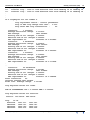
Sample processing report
Calculating theoretical gravity for all data base points
-------------------------------------------------------Latitude field
: D:/cookbook/gravity/datasets/Survey9705/Latitude
Calculated gravity field: D:/cookbook/gravity/datasets/Survey9705/theograv
Gravity datum
: IGSN71
Gravity units
: Milligals
To convert data reduced to a different ellipsoid:
You may want to merge two datasets that were reduced to different ellipsoids. If the
datasets do not contain an observed gravity field you can use this option to revert to
observed gravity for one of the datasets. You can then reduce the observed gravity to
the required ellipsoid as usual.
1
From the Settings menu, select the datum that was used for the original
reduction. Choose Theoretical Gravity to calculate the theoretical gravity that
was subtracted from the observed gravity using this ellipsoid.
2
Use the spreadsheet editor to reapply (add) the theoretical gravity to the corrected
gravity field to recreate the observed gravity field obsgrav. See Step 2 of the
complete Bouguer worked example in Gravity field reduction and correction (C08)
for an example of using the Spreadsheet tool.
3
Select your preferred datum from the Settings menu (for example WGS84).
Calculate the theoretical gravity using this preferred datum.
4
Use the spreadsheet editor to subtract the revised theoretical gravity from the
observed gravity.
Theoretical gravity formula
Older gravity datums approximate normal gravity using truncated polynomial
expansions. Recent gravity datums use Somiglianas closed form solution.
For POTSDAM and IGSN71_AGSO
Gn = a1 * ( 1 + a2 * sin2φ + a3 * sin2(2φ) )
For IGSN71 and ISOGAL80
Gn = a1 * ( 1 + a2 * sin2φ + a3 * sin4φ )
For WGS84 and GA07 (GRS80)
2
( 1 + a 2 ( sin φ ) )
G n = a 1 -----------------------------------------2
( 1 + a 3 ( sin φ ) )
Where
Gn is theoretical gravity in µms–2
φ represents degrees of latitude
Library | Help | Top
© 2012 Intrepid Geophysics
| Back |
INTREPID User Manual
Library | Help | Top
Gravity corrections (T54)
12
| Back |
a1, a2, a3 are constants listed in the table of constants. See Gravity constants for
various datums.
R0 is the mean radius of the earth
Free air anomaly
Parent topic:
Utility gravity
transforms
The free air correction compensates the observed gravity for the fact that it was
measured at a given height above (or below) the datum.
It assumes, however, that there is nothing but air between the geoid or ellipsoid and
the observation point.
INTREPID calculates the free air correction from the elevation and observed gravity
fields and the terrain type.
The free air anomaly is calculated as follows:
FreeAir = obsgrav - theoretical gravity - free air correction
o b sg ra v
S u b tra c t
t h e o r e t ic a l
g r a v it y
S u b tra c t
fr e e a ir
c o r r e c t io n
F r e e A ir
E le v a t io n
Input field
obsgrav, Latitude, Elevation
Output field
FreeAir
Free air correction formula
Here is the formula for free air correction using the full formula expressed as a
vertical gradient.
For POTSDAM and IGSN71_AGSO
δgh = – 3.086 * h
For IGSN71 (GRS67)
δgh = – (3.08768 – 0.00440 sin2φ ) * h + 0.000001442 * h2
For ISOGAL80
δgh = – 3.086 * h + 7.3 * 10–8 * h2
For WGS84
δgh = – (3.083293357 + 0.004397732 * cos2φ) * h + 7.2125 * 10–7 * h2
For GA07 (GRS80)
δgh = – (3.087691 – 0.004398 sin2φ ) * h + 7.2125 * 10–7 * h2
Where
δgh is the free air correction to be subtracted, in μms–2 per metre
h is the height of the gravity meter above the ellipsoid
φ represents degrees of latitude
Library | Help | Top
© 2012 Intrepid Geophysics
| Back |
INTREPID User Manual
Library | Help | Top
Gravity corrections (T54)
13
| Back |
Correction for the mass of the atmosphere
Mass of atmosphere is not included in theoretical gravity for datums older than
WGS84, thus there is no need to correct for it when calculating a free air anomaly.
This correction is automatically subtracted from the normal gravity
For POTSDAM, IGSN71_AGSO, IGSN71, ISOGAL80
δgatm = 0
For WGS84, stations above sea level:
δg atm = 8.7e
h 1.047
– 0.116 ⎛⎝ ------------⎞⎠
1000
For WGS84, stations below sea level:
δgatm = 8.7
For GA07 (GRS80)
δgatm = 8.74 – 0.000 99 * h + 0.000 000 035 6 * h2
Where
δgatm is the atmospheric correction in µms–2
h = height above ellipsoid (not sea level) in metres
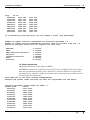
Sample processing report
Calculating Free Air Anomaly
---------------------------Observed gravity field
Latitude field
Station Elevation field
Meter
Elevation field
Output free air field
Gravity datum
Terrain type
Gravity units
:
:
:
:
:
:
:
:
D:/cookbook/gravity/datasets/Survey9705/obsgrav
Survey9705/Latitude
Survey9705/Elevation
NO METER ELEVATION DATA BEING USED
D:/cookbook/gravity/datasets/Survey9705/zzzz
IGSN71
land
Milligals
Reverse free air anomaly
Parent topic:
Utility gravity
transforms
Use this correction when your data contains a free air anomaly field but no observed
gravity field.
INTREPID adds the free air correction and the theoretical gravity to the free air
anomaly field to recreate the observed gravity field.
obsgrav = FreeAir + free air correction + theoretical gravity
Input field
FreeAir, Latitude, Elevation,
Output field
obsgrav
Sample processing report
Reversing Free Air anomaly to observed gravity.
----------------------------------------------
Library | Help | Top
© 2012 Intrepid Geophysics
| Back |
INTREPID User Manual
Library | Help | Top
Gravity corrections (T54)
14
| Back |
Free air gravity field
Latitude field
Station Elevation field
Meter
Elevation field
Output gravity field
Gravity datum
Terrain type
Gravity units
:
:
:
:
:
:
:
:
D:/cookbook/gravity/datasets/Survey9705/FreeAir
Survey9705/Latitude
Survey9705/Elevation
NO METER ELEVATION DATA BEING USED
D:/cookbook/gravity/datasets/Survey9705/obsgrav
IGSN71
land
Milligals
Simple Bouguer anomaly
Parent topic:
Utility gravity
transforms
The simple Bouguer correction replaces the "air" in the Free Air anomaly with matter
of a given density.
INTREPID uses the observed gravity field and the specified density and datum
settings to calculate the simple Bouguer correction.
The simple Bouguer anomaly is calculated as follows:
Bouguer = obsgrav – theoretical gravity – free air correction – simple Bouguer
correction
o b sg ra v
S u b tra c t
fr e e a ir
c o r r e c tio n
S u b tra c t
th e o r e tic a l
g r a v ity
L a titu d e
S u b tra c t
Bouguer
c o r r e c tio n
Bouguer
E le v a tio n
U n its
d a tu m
t e r r a in t y p e
d e n s ity
d a tu m
Input field
obsgrav, Latitude, Elevation
Output field
Bouguer
You can experiment with different density settings to create a series of simple
Bouguer anomaly fields; for example Bouguer267, Bouguer250, Bouguer200.
Simple Bouguer correction formula (spherical cap)
For GA07 (GRS80), the simple Bouguer correction is calculated using the following
closed form equation for the gravity effect of a spherical cap of radius 166.7 km with a
mean radius of 6,371.0087714 km, and height relative to the ellipsoid:
Bouguer Correction (BC) = 2πGρ((1+μ) * h – λR)
Where:
π is pi
G is the gravitational constant; = 6.67428 x 10–11 m3kg–1s–2
(Mohr and Taylor 2001)
ρ is density in tm–3, typically 2.67 tm–3
h is the ellipsoid height in metres of the station
R = (Ro + h) the radius of the earth at the station
Ro is the mean radius of the earth = 6,371.008 771 4 km
(GRS 80 value from Moritz)
μ & λ are dimensionless coefficients with following definitions:
Library | Help | Top
© 2012 Intrepid Geophysics
| Back |
INTREPID User Manual
Library | Help | Top
Gravity corrections (T54)
15
| Back |
μ = ((1/3) * η2 – η)
where
η = h/R
λ = (1/3){(d + fδ + δ2)[(f – δ)2 + k]1/2 + p + m*ln(n/(f – δ + [(f – δ)2 + k]1/2)}
where:
d = 3cos2α – 2
f = cos α
k = sin2α
p = –6cos2αsin(α/2) + 4sin3(α/2)
δ = Ro/R
m = –3sin2αcos α = –3kf
n = 2[sin(α/2) – sin2(α/2)]
α = S/Ro, with S = Bullard B Surface radius = 166.735 km.
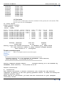
Sample processing report
Calculating Simple Bouguer Anomaly
---------------------------------Observed gravity field : D:/gravity/import_data/Survey9533_0710/Bouguer
Latitude field
: D:/gravity/import_data/Survey9533_0710/Latitude
Station Elevation field : D:/gravity/import_data/Survey9533_0710/Elevation
Meter Elevation field : NO METER ELEVATION DATA BEING USED
Bouguer anomaly field : D:/gravity/import_data/Survey9533_0710/Bouguer2
Gravity datum
: IGSN71
Terrain type
: land
Density
: 2.670
Gravity units
: Milligals
Reverse simple Bouguer anomaly
Parent topic:
Utility gravity
transforms
INTREPID calculates the observed gravity from the simple Bouguer gravity anomaly
field.
obsgrav = Bouguer + simple Bouguer correction + free air correction + theoretical
gravity
Input field
Bouguer, Latitude, Elevation
Output field
obsgrav
This is useful if you have data that is missing an observed gravity field and want to
process it using different settings or corrections.
Sample processing report
Calculating Simple Bouguer Anomaly
Reversing Simple Bouguer anomaly to observed gravity
---------------------------------------------------Bouguer anomaly field
Latitude field
Library | Help | Top
: D:/cookbook/gravity/datasets/Survey9705/Bouguer
: Survey9705/Latitude
© 2012 Intrepid Geophysics
| Back |
INTREPID User Manual
Library | Help | Top
Gravity corrections (T54)
16
| Back |
Station Elevation field
Meter
Elevation field
Output gravity field
Gravity datum
Terrain type
Density
Gravity units
:
:
:
:
:
:
:
Survey9705/Elevation
NO METER ELEVATION DATA BEING USED
D:/cookbook/gravity/datasets/Survey9705/obsgrav
IGSN71
land
2.670
Milligals
Eötvös gravity correction
Parent topic:
Utility gravity
transforms
The Eötvös correction is required for gravity measurements taken from a moving
platform. The meter's velocity over the surface adds vectorially to the velocity due to
the earth's rotation, varying the centrifugal acceleration and hence the apparent
gravitational attraction. Use this correction for marine and airborne survey data
before applying Latitude and FreeAir corrections.
L a t it u d e
lin e b e a r in g
c a lc u la t e
E ö tv ö s
c o r r e c t io n
E o tv o s
c r a f t v e lo c it y
U n it s
Input field
Latitude, line bearing and craft velocity
Output field
Eotvos
WARNING: The craft velocity is in units of knots!
Sample processing report
Calculating Eotvos gravity for all data base points
--------------------------------------------------Latitude field
:
Line bearing field
:
Craft velocity field
:
Calculated Eotvos field:
Gravity units
:
D:/cookbook/gravity/datasets/Survey9705/Latitude
D:/cookbook/gravity/datasets/Survey9705/bearing
D:/cookbook/gravity/datasets/Survey9705/velocity
D:/cookbook/gravity/datasets/Survey9705/Eotvos
Milligals
Applying the correction
The Eötvös correction is positive when the craft is moving to the east (because when it
moves with the earth, centrifugal acceleration is increased and the downward pull is
decreased) and negative when its motion is westward.
Use the spreadsheet editor to add the Eötvös correction to your observed gravity field
to create a new Eötvös corrected gravity field. See "Complete Bouguer anomaly—
worked example" in Gravity field reduction and correction (C08) for an example of
using the Spreadsheet tool.
Velocity from Eötvös gravity correction
Parent topic:
Utility gravity
transforms
Library | Help | Top
Given the Eötvös correction, line bearing and latitude, using this option INTREPID
computes the craft velocity that was required to produce just that Eötvös effect.
© 2012 Intrepid Geophysics
| Back |
INTREPID User Manual
Library | Help | Top
Gravity corrections (T54)
17
| Back |
Input field
Latitude, line bearing and Eötvös correction
Output field
craft velocity
WARNING:
•
The Eötvös correction is in units of milligals.
•
INTREPID computes the craft velocity in units of knots.
Sample processing report
Calculating velocity from Eotvos gravity for all data base points
----------------------------------------------------------------Latitude field
Line bearing field
Calculated velocity
Eotvos field
Gravity units
:
:
:
:
:
D:/cookbook/gravity/datasets/Survey9705/Latitude
D:/cookbook/gravity/datasets/Survey9705/bearing
D:/cookbook/gravity/datasets/Survey9705/velocity
D:/cookbook/gravity/datasets/Survey9705/Eotvos
Milligals
Gravity constants for various datums
Parent topic:
Utility gravity
transforms
Datum
The following table shows the constants used in theoretical gravity formulas
a1
a2
a3
R0
9780490.0
0.0052884
–0.0000059
6371229.3154
IGSN-71_AGSO
9780318.46
0.0053024
0.0000058
6371031.5014
IGSN-71
9780318.456
0.005278895
0.000023462
6371031.5014
9780332.7
0.005278994
0.000023461
6371008.7714
9780326.7714
0.00193185138639
–0.00669437999013
6371008.7714
1930 &
POTSDAM &
ISOGAL65
formula
coefficients
POTSDAM
1967 &
ISOGAL84
formula
coefficients
World Geodetic
System 1972 &
WGS80 formula
coefficients
ISOGAL80
World Geodetic
System 1984 &
WGS84 formula
coefficients
WGS84
Library | Help | Top
© 2012 Intrepid Geophysics
| Back |
INTREPID User Manual
Library | Help | Top
Datum
Gravity corrections (T54)
18
| Back |
a1
a2
a3
R0
9780326.7715
0.001931851353
–0.00669438002290
6371008.7714
GA07 formula
coefficients
GA07
Terrain correction
Parent topic:
Gravity
corrections
(T54)
The complete Bouguer anomaly reduction includes the simple Bouguer slab
correction, earth curvature correction and terrain correction. The INTREPID
complete Bouguer anomaly option calculates a terrain response for gravity data.
You must provide a digital terrain model (DTM) grid which is used to calculate the
terrain correction required for each gravity station. After the terrain correction has
been calculated, the correction can be applied to the Bouguer anomaly using the
INTREPID spreadsheet editor.
Terrain correction can be calculated for either land, marine or airborne data. Full
tensor gravity terrain corrections for new generation data acquisition systems are
also supported. Use this option also for Falcon, then use the spreadsheet functions to
re-organise the FTG tensor to create a Falcon tensor. Generally, it is best to assume a
1 g/cc density for the terrain correction phase, then use the spreadsheet editor, to
scale the terrain correction with a variety of density values, to minimize the
correlation of the observed gravity signal with the terrain response. This principle
applies even more so for gradiometry, as from experience, 80% of the measured signal
is usually due to the terrain response.
Gravity tool licensing
Parent topic:
Terrain
correction
If you are licensed for Gravity 1, you can calculate normal vertical gravity terrain
corrections for land, airborne and marine environments.
If you are licensed for Gravity 2, you can calculate normal vertical and horizontal
component gravity terrain corrections, as well as full tensor terrain corrections for
land, airborne and marine environments.
Scalar terrain corrections
Parent topic:
Terrain
correction
When simple Bouguer gravity anomalies are calculated for land gravity data, the
gravity station is assumed to be located on a horizontal plane. This assumption is
wrong if there is local varying topography. In this case a terrain correction must be
applied to the data.
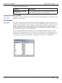
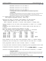
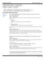
The terrain correction algorithm divides the region surrounding a gravity station into
concentric rings of increasing radii. Each ring, labelled A, B and C in the figure below,
is subdivided into cells. These cells are smallest in the innermost ring and increase in
size with each ring (similar to the well-known Hammer method for terrain
corrections).
A mean elevation is assigned to each cell and prisms are formed by projecting the
cells up or down to the station elevation plane which corresponds to the top of the
simple Bouguer slab. This is schematically shown in the figure below for a few
prisms.
Library | Help | Top
© 2012 Intrepid Geophysics
| Back |
INTREPID User Manual
Library | Help | Top
Gravity corrections (T54)
19
| Back |
A
B
C
Station elevation = thickness of
Bouguer slab
Gravity
Station
Reference Level
Prisms in the innermost ring (A) have a sloping top to better adapt to terrain
variations within a cell. The gravity effect of prisms in outer rings (B, C) is calculated
using a vertical rod approximation to speed up the computation. Each prism is
assigned a standard density and the terrain correction is calculated at each station as
the sum of effects due to all prisms contained within the radii. This provides
maximum precision in the region nearest to the station, while allowing more efficient
calculation further away.
To prevent edge effects, you should choose a DTM that is larger than your survey
area. For best results, your DTM should be large enough so that for each gravity
station the area used to calculate the terrain correction is completely contained
within the DTM.
In areas of high relief terrain corrections can be quite high. In Australia, gravity
terrain corrections can be as high as 25 mGal, and the terrain effect can extend for 50
km.
The terrain correction is added to the simple Bouguer anomaly to produce the
Complete Bouguer anomaly. In the case of land gravity the terrain correction is
positive everywhere. This is not necessarily true for airborne and marine terrain
corrections.
Please note that INTREPID calculates the scalar terrain correction using the
common convention that the vertical component of gravity is positive (the z-axis is
pointing down).
A full description of the terrain correction method used in the INTREPID software
can be found in the following reference: 'Application of terrain corrections in
Australia' by N. Direen, T. Luyendyk, Geoscience Australia (see Application of terrain
corrections in Australia (C13)).
Tensor terrain corrections
Parent topic:
Terrain
correction
The algorithm to calculate the terrain correction for full tensor gravity gradiometry
data is essentially the same as in the scalar case. However, there is one distinct
difference:
It is well known that for land-based gravity measurements the simple Bouguer
correction overestimates the gravity effect of the material between the gravity station
and the reference level (geoid or ellipsoid) in the presence of significant relief. The
terrain correction accounts for this by calculating the effect of missing or excess mass
due to variations in topography. On the other hand, the gravity effect of a infinite
Bouguer slab is independent of the location and height of a gravity station on or above
Library | Help | Top
© 2012 Intrepid Geophysics
| Back |
INTREPID User Manual
Library | Help | Top
Gravity corrections (T54)
20
| Back |
the slab. The gradient tensor response of a Bouguer slab is thus identical to zero
everywhere and the concept of a simple Bouguer correction is not applicable in the
tensor case.
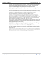
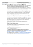
Instead, a forward model of the terrain has to be calculated to account for effects of
topography on the gravity tensor. As with the scalar case, the terrain surrounding the
gravity station is divided into prisms. The prisms extend from a reference level,
usually the geoid or ellipsoid, to the terrain elevation (cf. the figure below). In the
innermost ring sloping top prisms are used for high accuracy, whereas flat-top prisms
are used in the outer rings to speed up the computation. A density is assigned to each
prism and the tensor terrain correction at a gravity station is given as the sum of the
gradient tensor response from all prisms inside the concentric rings.
A
B
C
Gravity
Station
Reference Level
With the evaluation of the tensor terrain correction, a forward model of the full
gravity vector is also calculated. Note, that the vertical component of the gravity
vector is different to the value from the scalar terrain correction. The former is the
response of a complete forward model, whereas the latter accounts for the mass
missing from or in excess of an infinite Bouguer slab.
Finally, the tensor terrain correction has to be subtracted from the tensor data to
remove the effect of topography. This can be done using the spreadsheet editor.
Note: The full gravity vector and the gravity gradient tensor are calculated in the
ENU coordinate system, i.e. the x-axis points east, the y-axis points north and the zaxis points up.
You have to convert the tensor terrain correction first before you can subtract it from
your gravity gradient tensor data if the latter is expressed in a different coordinate
system such as NED (north-east-down) or END (east-north-down).
Computing a terrain correction
Parent topic:
Terrain
correction
Library | Help | Top
From the Process menu, select Terrain Correction anomaly.
© 2012 Intrepid Geophysics
| Back |
INTREPID User Manual
Library | Help | Top
Gravity corrections (T54)
21
| Back |
The Mode box requires you to choose appropriate settings for the gravity Datum,
units, and survey environment. After you select the correct modes the main dialog box
appears.
Library | Help | Top
© 2012 Intrepid Geophysics
| Back |
INTREPID User Manual
Library | Help | Top
Gravity corrections (T54)
22
| Back |
Parameters
Parameter
Description
Earth Curvature
Correction
Converts the geometry for the correction from an infinite
slab to a spherical cap with a radius of 167 km from the
station. Select this option if your survey covers a wide area.
This only applies to scalar terrain corrections.
Calculate Scalar
Terrain correction
This is the default setting. INTREPID calculates the
terrain correction for the vertical component of gravity.
Calculate Full
Tensor correction
Id you select this option, INTREPID calculates a full tensor
terrain correction together with all components of the
gravity vector.
Note that the gravity gradient tensor is in the ENU system.
Note that tensor terrain corrections compute a forward
model of the gravity tensor based on the DTM at each
observation point. This is different to scalar correction,
which computes the effect of the deviation from the infinite
slab or spherical cap approximation.
You must be licensed for Gravity 2 to use this option.
Number of
Calculation Rings
These are the rings of terrain influence surrounding the
observation point. Specify a range between 1 and 5.
Choosing fewer rings provides less coverage but faster
processing. Choosing 5 rings gives maximum coverage and
maximum accuracy but slower processing. The radius of
the area processed approximately doubles for each outer
ring if you use default settings. Remember that most of the
terrain influence occurs in the inner rings close to the
station.
Primary Cell Size
Controls the prism cell size which is used to model the
terrain surface. This parameter depends on the resolution
of the DTM grid. It also controls the radius of each ring (See
the Advanced options below). Specify the DTM grid cell
size to start with. Increasing the size increases the ring
radii. The result is less accurate but it runs faster.
Density (Land)
The density in g/cm3 assigned to prisms on land.
Density (Seawater)
The density in g/cm3 assigned to prisms in the sea
Advanced options
Library | Help | Top
Setting
Description
Terrain Bottom (RL)
Full tensor gradient terrain corrections for land/air/
sea are supported. The Holstein polyhedra
modelling method is used to calculate the tensor
response of the terrain. The method requires a
bottom RL to determine the height of the prisms.
© 2012 Intrepid Geophysics
| Back |
INTREPID User Manual
Library | Help | Top
Gravity corrections (T54)
23
| Back |
Setting
Description
Radius (in cells) of Ring
1:5
The radius of the rings of terrain influence (in
primary cell sites) can be individually modified.
Calculate scalar/tensor
terrain corrections
using...
The method of sloping prisms is the more accurate
but slower option. Note that this only affects the
prisms in the innermost ring. Outer rings always
use the rod approximation pscalar cape ?? or flat top
prisms (tensor case)
Press the first Browse button to select your gravity
dataset. Press the second Browse button to select
your DTM grid. Press the third Browse button to
optionally select a name for your output report file.
You hve the option of writing the calculated terrain
values to the report file.
Treatment of Elevation
Observation Data
For ground gravity data, if the elevations calculated
from the DTM differ significantly from those
measured with the gravity readings, the option
exists to replace all station elevations by those
interpolated from the DTM grid for calculating the
terrain correction. This is the default setting.
Note: Do not replace observation elevation if you
are processing airborne or marine data.
Include Observation Point
in DTM
The elevation at each gravity station location must
be estimated by interpolating from the DTM grid.
You have the option of including the gravity reading
elevations along with the DTM data for the
interpolation process. The default setting is not to
do this.
Local elevation
interpolation method
The interpolation of the elevation can be done using
the method of either inverse distance (default) or
minimum curvature.
Press Finish. You are now prompted for a flag field. This can be any field in the
dataset which contains valid data. If the field contains any Null values, INTREPID
skips the terrain calculation for those records.
INTREPID asks you for the ground elevation field relative to the geoid. You can also
specify an optional meter elevation relative to the geoid. Press Skip if you do not have
one. You can also specify an optional gravity units field. Press Skip if you do not have
one.
Now specify the output terrain correction field name. The default name is
compl_boug. Choose OK. INTREPID starts calculating the terrain correction.
After INTREPID has computed the terrain correction, you may use the INTREPID
spreadsheet editor to add it to the simple Bouguer anomaly to create the complete
Bouguer anomaly.
Library | Help | Top
© 2012 Intrepid Geophysics
| Back |
INTREPID User Manual
Library | Help | Top
Gravity corrections (T54)
24
| Back |
Note however, if you are dealing with tensor data, the tensor terrain correction has to
be subtracted from the full tensor data.
See "Complete Bouguer anomaly—worked example" in Gravity field reduction and
correction (C08) for more information on the technical capabilities.
Gravity mode settings
Parent topic:
Gravity
corrections
(T54)
You can use the help menu to display help text on the topics shown in the menu
illustration below.
You can change a number of INTREPID settings during a Gravity processing session.
Every time a dataset containing Gravity data is referenced, you must explicitly
confirm the following essential information. This ensures that the units, geoid,
ellipsoid and equations that you are expecting to use, are in fact the ones chosen.
While elements of gravity data reduction appear simple, it is a known fact, that many
practitioners generate anomaly numbers that are difficult to reproduce, as a simple
mistake has been made in choosing the right parameters.
Library | Help | Top
© 2012 Intrepid Geophysics
| Back |
INTREPID User Manual
Library | Help | Top
Gravity corrections (T54)
25
| Back |
Settings and formats
Setting or format
Description
AGSO format
You are prompted for data file names, output report
file name, and output database names.
Scintrex formats
You are prompted for data file names, output report
file name, and output database names.
Survey Number
Used to extract just that survey number from the data
file.
Survey Suffix
Only relevant for the formal AGSO import, you may
ignore it
Override meter
settings regarding
coordinate type
Usually the values coming out of the meter are
showing LatLong, though in other cases they may be a
local grid, or UTM coordinates.
Gravity Datum Type
This is one of Potsdam, IGSN71, IGSN71_AGSO,
IGSN71_NZ, ISOGAL80, WGS84, GA07.
INTREPID uses the standard International Formulae
and there are references to regional tie-ins. You can
easily define new Datums as required. Please contact
technical support with details of any other required
tie-ins.
Output Gravity Units
INTREPID uses either mGal, µms–2, or µGal. Specify
the units used in the data you intend to import or
process before you start the process. The default unit is
mGal. One milligal (mGal) = 10 µms–2
Gravity Acquisition
Environment
INTREPID uses different processing parameters for
land, marine and airborne gravity data. You can select
Land, Marine, Airborne, Lake or Ice.
The default environment is Land.
Specifying input and output files
Parent topic:
Gravity
corrections
(T54)
You can use the help menu to display help text on the topics shown in the menu
illustration below.
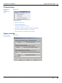
Introduction to input and output files.
In each case INTREPID displays an Open or Save As dialog box. Use the directory
Library | Help | Top
© 2012 Intrepid Geophysics
| Back |
INTREPID User Manual
Library | Help | Top
Gravity corrections (T54)
26
| Back |
and file selector to locate the file you require. (See "Specifying input and output files"
in Introduction to INTREPID (R02) for information about specifying files).
Menu options
Option
Description
Open Gravity
Database
Use this to specify the gravity dataset which you wish to
manipulate. You may perform utility gravity transforms
and terrain corrections on an existing gravity dataset.
It is also possible to open an XYZ or an existing principal
facts database and make use of some of the data
reduction and network adjustment tool functions. In this
case only some of the processing sequence can be applied
to the data. In this case you cannot then answer
questions about differing precision of one reading vs
another, because Gravity datum changes etc. so easily.
Survey Import Wizard
The Import Wizard is the starting point for reduction and
network adjustment of field data in AGSO or Scintrex
format.
Dump / Check CG5
Convert binary format CG5 data to readable ASCII.
Useful for viewing the data before importing.
Merge new survey
with master database
The Gravity Tool allows you to merge your current
dataset with a ‘master’ dataset of principal facts. Fields to
be merged must have the same names. Missing fields are
set to Null values.
This option calls a separate tool called "merge.exe" that
does location and precision checks on the new data
compared to the master data, and attempts to arbitrate,
or make a judgement about which records are better.
Exceptions are written to a log file for reprocessing/
editing. Do not use this option without some planning and
thought. Check the tutorial first.
Library | Help | Top
Edit Gravity Database
Aliases
This supports normal assigning and re-assigning of the
standard INTREPID alias names.
Load Options
Select a Grdop task specification file to preload the
interactive session with all the required file and
parameter settings. (See Using task specification files for
information about task specification files).
Save Options
Save the current Grid Operations file specifications and
parameter settings as a task specification file. (See
Section Using task specification files for more
information).
© 2012 Intrepid Geophysics
| Back |
INTREPID User Manual
Library | Help | Top
Gravity corrections (T54)
27
| Back |
Process menu
Parent topic:
Gravity
corrections
(T54)
Intro text
In this section:
•
Reduce loop data
•
Gravity transforms
•
Complete Bouger anomaly
•
Complete Bouger anomaly advanced options
•
Create tensor from inline or crossline
•
Create inline or crossline from tensor
Reduce loop data
Parent topic:
Process menu
Library | Help | Top
Intro text
© 2012 Intrepid Geophysics
| Back |
INTREPID User Manual
Library | Help | Top
Gravity corrections (T54)
28
| Back |
Controls in this dialog box
Control
Description
Gravity loop database
This is the intermediate database, with standardised
fields, that capture intermediately processed field
data, still in LOOP order
Control gravity
observations database
Your tie-in to a national datum, or an absolute station,
is kept in a much smaller, seperate database. This is
not strictly necessary, but your survey data cannot be
interpreted or merged with other surveys, until this is
done properly.
Output database
The final principal facts data reduction from your
newly acquired survey, get written using standard
feild names, to this output gravity database.
Output report
A very comprehensive report, that pulls all your data
apart, reporting on loop design, repeats, drifts, error
analysis, is automatically written by the tool to this
file. Please examine it carefully.
Gravity transforms
Parent topic:
Process menu
These calculator functions require supporting fields to function correctly, and you
also need to know the gravity datum, if you wish for example, to revese back to an
observed gravity value from a FreeAir. Some of the prompted fields are optional
extras. A SKIP button will present in this case.
Before a final calculation is executed, after you have been prompted for all the
necessary fields to conduct your required calulation, you will get a summary pop-up
describing what you are attempting to do. Please check and verify that what this
reports, is what you intended to do.
Library | Help | Top
© 2012 Intrepid Geophysics
| Back |
INTREPID User Manual
Library | Help | Top
Gravity corrections (T54)
29
| Back |
Controls in this dialog box
Control
Description
Select gravity operation
Choose one of the 8 options above
Output database
Any database can be used to manage/
manipulate gravity observations. The
importance of these calculator functions is
that data from any source and age can have
reverse forumulae applied, say reverse out
of Potsdam, then go forward to ISOGAL.
This also applies to the moving platform
Eotvos correction.
Complete Bouger anomaly
Parent topic:
Process menu
Library | Help | Top
Intro text
© 2012 Intrepid Geophysics
| Back |
INTREPID User Manual
Library | Help | Top
Gravity corrections (T54)
30
| Back |
Controls in this dialog box
Library | Help | Top
Control
Description
Earth curvature correction
For a scalar terrain correction, the
correction at 167km and further, is the
traditional Earth curvature correction.
Calculate scalar terrain
correction
This is the classic case, with rods and
sloping top triangle prism modelling
Calculate full tensor
correction
This terrain modelling uses the Holstein
facet modelling code for a FTG case.
Number of calculation
rings
Tis comes from the Hammer chart idea of 2
to 5 rings. The primary contribution comes
from the closest terrain and this falls in the
inner ring
Primary cell size
This cell size is independent of the
underlying DTM grid, as a resampling is
used. This drives the actual radius for each
ring, as the cell size is multiplied by the
number of cells in each ring.
Density
This is the assumed terrain or regolith
density value. If you use 1 g/cc, you can scale
the calculated field later in thye spreadsheet
Gravity database
The observed gravity database must include
a field for the observation points ( X,Y,Z). It
is not actually necessary to have the actual
observed field, as the aim here is to create a
field with the terrain correction fields,
without actually applying the corrections at
this point in the process.
Digital terrain model grid
This is a standard geophysical grid that has
the local DTM, with good extents, far
beyond the gravity observation stations.
SRTM can be OK, but generally something
with better resolution is required.
Output report
A very comprehensive report is created
every time this option is run. A full
explanation of all the options is recorded in
this report.
© 2012 Intrepid Geophysics
| Back |
INTREPID User Manual
Library | Help | Top
Gravity corrections (T54)
31
| Back |
Control
Description
Treatment of elevation
observation data
Interestingly, the accuracy of the survey
height of the gravity observation station,
often is out of sorts with the DTM grid, so
the option exists to locally adapt the DTM to
include the local survey heights. However,
this may not work, and you may have to
settle for the DTM view of the elevation at
the station to avoid “pimples”
Local elevation
interpolation method
If you want to use the local observation of
elevation, and mix this with the DTM, this
requires a local interpolation - two methods
are available, inverse distance squared and
a MINQ.
Complete Bouger anomaly advanced options
Parent topic:
Process menu
Library | Help | Top
Here is finally where the ring dimensions are finalised. The radius of the inner ring is
16 * cellsize. This inner ring is always carefully modelled with high resolution prisms,
and the option for sloping top prisms does make quite a difference.
© 2012 Intrepid Geophysics
| Back |
INTREPID User Manual
Library | Help | Top
Gravity corrections (T54)
32
| Back |
Controls in this dialog box
Control
Description
Terrain bottom
For the tensor case, a notional bottom RL is also
required. make this well below the terrain elevation.
Radius of rings
The ratio of 16,32,64,256,1024 is the traditional
scalar gravity ratios. As gradiometry falls off by one
oredr of magnitude greater than scalar gravity, a
different ratio series with a sharper roll off is
recommended. eg use a finer cellsize and 9,27,81,243.
Calculate scalar/tensor
terrain correction using
It is recommended you start with flat top prisms and
just 2 rings to make sure all is looking as it should, eg
the DTM grid is appropriate and the order of the
terrain correction seems in order. Then repeat the
process with a higher number of rings and use the
sloping top option.
Create tensor from inline or crossline
Parent topic:
Process menu
If you have FTG data from the contractor that is close to what was actually measured,
you may also have inline and crossline fields, often called I1,I2,I3, C1,C2,C3. You also
need a carousel angle, which captures the angular oreintation of the rotating GGI’s
within the Lockhead-Martin instrument. use the advanced alias assigment in the
ProjectManager tool to set these fields in your database, to the corresponding alias.
This must be done before you can successfully recreate the tensor field from its parts.
Choose this option, specify the output tensor field name, and the option to form the
tensor takes very liuttle time to compute. Note that FTG data from this instrument is
universally declared and formed in a left handed coordinate reference frame with
East/North/Down.
The tensor training coyurse contains a great trouve of practical information about
the details of all the gradient instruments in use today.
Library | Help | Top
© 2012 Intrepid Geophysics
| Back |
INTREPID User Manual
Library | Help | Top
Gravity corrections (T54)
33
| Back |
Controls in this dialog box
Controls
Description
Enter new field name
required name for the formed tensor field
Existing fields
Use the alias facility as described above to tie the
observed inline and crossline fields , whatever they
are named, to their function.
Create inline or crossline from tensor
Parent topic:
Process menu
This is the reveres process to the option above. Given a FTG field, decompose it back
to its inline and crossline parts, with the carousel angle held constant to an azimuth
of 0 degrees.
Controls in this dialog box
Control
Description
Input tensor
field
Choose any tensor field in your database,
and recompute equivalent inline and
crossline components.
Tools menu
Parent topic:
Gravity
corrections
(T54)
This collection of functions tend to be to the side of mainstream gravity processing.
In this section:
Library | Help | Top
•
Gravity meter calibration
•
Earth tides
•
Convert to WGS84
•
Convert Potsdam to IGSN71
© 2012 Intrepid Geophysics
| Back |
INTREPID User Manual
Library | Help | Top
•
Gravity corrections (T54)
34
| Back |
Sort database
Gravity meter calibration
Parent topic:
Tools menu
The AGSO field data format is designed to accomodate gravity readings collected
from calibration ranges. Using the known calibrated gravity stations, INTREPID can
calculate new instrument (scale) factors, and can optionally apply these to all the
gravity readings during the data reduction and network adjustment process.
Calibration and scale factor results are written to Section 3 of the processing report.
See Gravimeter calibration (R29) for details.
Contact INTREPID if you wish to have access to examples of land gravity meter
calibrations.
Controls in this dialog box
Controls
Description
AGSO gravity field data
An ASCII file that contains field observations
from a calibration exercise, so there are many
repeats, and possibly 2 or more meters, occuping
several well known and observed gravity
stations.
Output report
standard report file for capturing results
Earth tides
Parent topic:
Tools menu
Most gravity field data format is designed to accomodate earth tides. The value of
gravity at any point on the Earth varies during the course of the day because of the
tidal attraction of the sun and the moon. INTREPID automatically applies Earth tide
corrections during the data reduction and network adjustment process. INTREPID
uses the Longman formula.
Earth Tide corrections may also be calculated manually, and the results written to a
report file.
Select Earth Tides from the Tools menu.
Specify the location and time interval. Specify the name of the report file.
Library | Help | Top
© 2012 Intrepid Geophysics
| Back |
INTREPID User Manual
Library | Help | Top
Gravity corrections (T54)
35
| Back |
Controls in this dialog box
Controls
Description
Title
A title
Latitude
where on the earth
Longitude
where on the earth
Elevation
where on the earth
Month
what month are you interested in?
Year
what year are you interested in?
Interval
dump values for every interval in minutes
Time difference
offset in time from GMT
Convert to WGS84
Parent topic:
Tools menu
Library | Help | Top
Use this to convert an Observed gravity field from a non-WGS84 gravity datum to the
WGS84 gravity datum. Specify the new gravity field name in the Specify Output
Observed Gravity Field dialog box.
© 2012 Intrepid Geophysics
| Back |
INTREPID User Manual
Library | Help | Top
Gravity corrections (T54)
36
| Back |
Controls in this dialog box
Controls
Description
Specify input observed
gravity field
You are prompted for an observed gravity field in
your database, together with its datum
Convert Potsdam to IGSN71
Parent topic:
Tools menu
Use this to convert an Observed gravity field from the Potsdam gravity datum to the
IGSN71 gravity datum
Sort database
Parent topic:
Tools menu
Sort the database on any indexed field. Sorting the database on Station number is a
useful way of checking for repeat stations. The INTREPID database format is very
flexible. The primary focus is its ability to handle groups of fields, associated with a
profile. With the classic random point nature of a regional gravity database, the
default key fields, such as StationNumber, may conatin many duplicate readings, as
this field does not have to be a primary key.
In the standard field loop reduction process, the final principal facts process does
reduce the readings back to just one entry for each station. This function gives you
the ability to reorder the data rows, to force all the readings for each station to be in
order, when viewed in a spreadsheet, or dumped, via export, to an ASCII file.
Library | Help | Top
© 2012 Intrepid Geophysics
| Back |
INTREPID User Manual
Library | Help | Top
Gravity corrections (T54)
37
| Back |
Controls in this dialog box
Controls
Description
Sort groups
Function name
Indexed fields
Choose the field(s) that you want to sort the random
records in the database by. eg StationNumber
Sort keys
This is the chosen field(s) prior to the sort being
actually undertaken.
Spatial query
Parent topic:
Gravity
corrections
(T54)
Gravity data is collected often regionally, in temporal loops and spatial radom points.
You may suspect that data in one region has some sort of a drift or error, and you
wish to find the “outlier”.
This option allows you to drill down to individual stations by name, to lasso groups,
and to query in a temporal/spatial sense, the readings, so you can spot trends.
In this section:
•
Find gravity station
•
Trace a polygon
•
Load existing polygon
•
Save current polygon
•
Erase traced polygon
•
Pseudo profile view
Find gravity station
Parent topic:
Spatial query
Choose this option to get every entry in a “StationName” field to report. Click on an
entry in this list, and the background graphics window will show the requested
station in a purple highlight. This is a reverse search. Much the same can also be
done just simply typing the station name into the top right hand side text window,
followed by a carriage return.
A text convention is also used to indicate which stations are nodes and repeats, when
you have a processed field loop observation dataset loaded. The number of
connections above one to other stations, is recored by the “white” lines, and also the >, {}, (), ::, ## text code following the important stations.
Library | Help | Top
© 2012 Intrepid Geophysics
| Back |
INTREPID User Manual
Library | Help | Top
Gravity corrections (T54)
38
| Back |
Trace a polygon
Parent topic:
Spatial query
The aim here is to use the Spatial Query>Trace a polygon, to select a subset of the
gravity readings in a spatial sense, regardless of when the data was acquired, to
define a psuedo section for which a profile of gravity can be viewed.
Load existing polygon
Parent topic:
Spatial query
Library | Help | Top
Instead of doing on-screen digitizing of a polygon, you can choose an a existing
polygon dataset. This can come from anywhere, provided it meets the INTREPID
format requirements eg Arc shape file, something saved from the subset tool etc.
© 2012 Intrepid Geophysics
| Back |
INTREPID User Manual
Library | Help | Top
Gravity corrections (T54)
39
| Back |
Save current polygon
Parent topic:
Spatial query
You can save the polygon you have traced, to a polygon dataset, by choosing this
option. Provide a polygon dataset name. this is a standard polygon dataset, and can
also be saved in any GIS format.
Erase traced polygon
Parent topic:
Spatial query
This option simply erases the transient polygon graphic, and resets back to a neutral
state.
Pseudo profile view
Parent topic:
Spatial query
The longest dimension of the psuedo section is used to define an X axis. All the
gravity data points that lie within the polygon, are projected onto the section plot,
with the gravity reading as the Y axis. You can mouse click on any of the crosses
wiuthin this plot, to get a station report in the underlying RHS reporting pane. When
you have loop data, you can isolate individual field data records, to get to a seeming
outlier etc etc.
Settings menu
Parent topic:
Gravity
corrections
(T54)
To change a setting, choose a corresponding item from the Settings menu.
In this section:
•
Library | Help | Top
Tare detection limit
© 2012 Intrepid Geophysics
| Back |
INTREPID User Manual
Library | Help | Top
Gravity corrections (T54)
40
| Back |
•
Loop adjustment limit
•
Repeat rejection difference
•
Skip Earth tide correction
•
Strict view of nodes
•
Density
•
Gravity meter drift
•
Report detail
•
Database layout
•
Output datum
Tare detection limit
Parent topic:
Settings menu
A tare is an unacceptable difference between data acquired at successive stations. It
may be caused by a meter being knocked or dropped, and causes the subsequent
readings to be higher or lower than before.
The Tare Detection limit is the maximum acceptable tare. If a tare exceeds this value,
INTREPID insert a warning in the processing report file.
Controls in this dialog box
Controls
Description
Maximun tare
The default is 20 mGal, and this comes from experience
in the field. You would like to know if your meter
appears to have been bumped from one session to the
next.
Loop adjustment limit
Parent topic:
Settings menu
Library | Help | Top
The Loop Adjustment Limit is the limit of error for network adjustment corrections.
The loop adjustment stops when the maximum change for an iteration is less than the
specified limit. The default value is 0.01 mGal.
© 2012 Intrepid Geophysics
| Back |
INTREPID User Manual
Library | Help | Top
Gravity corrections (T54)
41
| Back |
Controls in this dialog box
Controls
Description
Maximum loop
adjustment
When doing a loop levelling adjustment, an iterative
improvement in the mis-fits will continue until the
maximum mis-fit is less than this limit. There is usually
no cause to change this value.
Repeat rejection difference
Parent topic:
Settings menu
This option sets the rejection tolerance value for repeat station values.
The default value is 0.20 mGal.
Controls in this dialog box
Controls
Description
Precision repeats
estimate
Enter a value to specify an acceptable difference between
readings at the same station.
Skip Earth tide correction
Parent topic:
Settings menu
Skip Earth Tide Correction
Turn off the Earth Tide correction. The default is to include it while doing the
standard land-based loop processing stream. This option also applies to marine
processing for L&R instruments etc. The workflow for this case, is tied up in batch
processing options for this tool, and is described in the marine gravity processing
cookbook.
Strict view of nodes
Parent topic:
Settings menu
Strict View of Nodes
A node (or tie) is defined as a station that appears in more than one loop. INTREPID
has two views of what constitutes a node:
1
Strict (rigorous) view
Station numbers that are repeated and arranged in time order are used as nodes.
The first and last stations in a loop are not used as nodes unless they are repeated.
Fixed stations are not used as nodes unless they are repeated.
2
Relaxed view
Station numbers that are repeated are used as nodes. All first and last stations in a
loop are used as nodes. All fixed stations are used as nodes.
The default setting is the Strict View of Nodes.
Library | Help | Top
© 2012 Intrepid Geophysics
| Back |
INTREPID User Manual
Library | Help | Top
Gravity corrections (T54)
42
| Back |
Density
Parent topic:
Settings menu
You can set the assumed density of material/terrain as appropriate. These values are
used for simple Bouguer and terrain corrections. Validate your choice in the pop-up
that is provided just before a calculation is done.
The default density for land is (2.67 g/cm3).
Controls in this dialog box
Controls
Description
Density
Enter a density value for the Bouguer slab correction. You
can specify land, sea, lake, marine sediment and ice
values.
Gravity meter drift
Parent topic:
Settings menu
INTREPID has a choice of two drift models:
•
The conventional short term linear drift uses a piecewise linear method to remove
the drift for each loop. The IgnoreRepeatsForShort option also allows you to
ignore repeat stations for the purpose of drift calculations.
•
Long term polynomial drift is calculated using a weighted least squares fit to the
nodes, with an outlier rejection criteria. A 2nd order drift rate curve is derived.
The area under this curve is found by integration and this is the model of the drift
adopted.
Long term polynomial drift is the default setting.
Library | Help | Top
© 2012 Intrepid Geophysics
| Back |
INTREPID User Manual
Library | Help | Top
Gravity corrections (T54)
43
| Back |
Options in this menu
Options
Description
Long-term
polynomial
Use a long term view of the metre drift, as modelled in a
piecewise polynomial drift curve, to help level the survey
Short-term linear
A short term linear drift curve is considered adequate for
most surveys. As you lean towards doing geodetic quality
work, switch to long-term drift modelling.
Ignore repeats
Variability at a station can distort gradients in the drift
curve, so trun off.
Report detail
Parent topic:
Settings menu
You can select brief or verbose processing reports.
The default setting is Brief.
See Gravity processing reports for details of the brief import and loop reduction
report.
The verbose processing report includes:
Section 1a—Check Print of positions.
The station number, latitude, longitude and height for each station.
Section 10—Earth tide corrections.
The Loop no, Station no, latitude, longitude, elevation, time, GMT, Earth tide and
adjusted gravity for each station.
Section 11.2—Final Drift Control Adjustments
Drift control data for each loop sequence.
Section 12.2—Loop Adjustments
Further detail about the loop adjustments.
Library | Help | Top
© 2012 Intrepid Geophysics
| Back |
INTREPID User Manual
Library | Help | Top
Gravity corrections (T54)
44
| Back |
Options in this menu
Options
Description
Brief
The default report type is brief, and is usually adequate
for all needs
Verbose
If a survey is giving you trouble and will not level very
weel, try turing on the extra reporting.
Database layout
Parent topic:
Settings menu
INTREPID writes a standard set of fields to the gravity datasets. The field names
follow the ASEG standard naming convention. All supporting fields are populated
directly by the program.
The Complete form of the layout contains additional fields created by the Terrain
Correction calculations.
The default setting is Standard. See INTREPID gravity point datasets (R28) for
details of fields.
Options in this menu
Options
Description
Standard
Geoscience Australia has defined a standard set of fields
for the principal facts gravity stations, available using
the GADDS web-based data delivery system. This is
powered by INTREPID JETSTREAM
Complete
Optional extra gravity fields can also be generated by the
processing within this tool, when doing field data
reduction.
Output datum
Parent topic:
Settings menu
Library | Help | Top
The spatial (XY) datum can be changed for output. It does not have to be the same as
the input spatial datum. Select the datum you require from the Select Datum dialog
box. For instance, all the land based survey loops maybe recorded using a GPS and
Latitude/Longitude pairs. At the very end of the processing, you may wish to present
the principal facts in a projected map format, with an Easting and a Northing.
© 2012 Intrepid Geophysics
| Back |
INTREPID User Manual
Library | Help | Top
Gravity corrections (T54)
45
| Back |
Options in this dialog box
Options
Description
Select datum
Select the Ellipsoid datum you wish to have the data
calculated in.
View menu
Parent topic:
Gravity
corrections
(T54)
Options for graphically displaying the drift of the gravimeter.
In this section:
•
Drift rate
•
Drift standard
•
Drift normalised
•
Screen dump to postscript
Drift rate
Parent topic:
View menu
This graph shows the drift rate for each tie in the first GMLS of the dataset( in this
case G132 & G651). This includes ALL ties (nodes); the ties at the beginning and end
of each loop (loop ties), and other ties within the GMLS. Use the Next and Previous
buttons to view other GMLS in the dataset.
The horizontal axis represents the time (days) since the survey began ( shown over
128 days). The vertical axis is the drift divided by the time difference (dial reading/
hr).
Library | Help | Top
© 2012 Intrepid Geophysics
| Back |
INTREPID User Manual
Library | Help | Top
Gravity corrections (T54)
46
| Back |
Drift standard
Parent topic:
View menu
This graph shows the drift for each loop in the first GMLS of the dataset. The
horizontal axis represents the time (days) since the survey began.The vertical axis is
the dial reading. Each line segment represents one loop. The length of the line
segment indicates the time taken to complete the loop. The gradient, if any, shows the
drift at the same node.
Drift normalised
Parent topic:
View menu
This graph shows the normalised drift for each loop in the first GMLS of the dataset.
The normalised graph shows each segment shifted up or down to fit a curve. This
gives some sense of a drift continuum for the GMLS.
The horizontal axis represents the time (days) since the survey began.The vertical
axis is the normalised dial reading. INTREPID fits a polynomial to the gradients
(drift) of the line segments (loops). It then shifts all line segments up or down so that
they start on this polynomial.
Library | Help | Top
© 2012 Intrepid Geophysics
| Back |
INTREPID User Manual
Library | Help | Top
Gravity corrections (T54)
47
| Back |
Screen dump to postscript
Parent topic:
View menu
Use the graphics engine within this tool, to create a postscript file with the loops,
stations layout.
Help
Parent topic:
Gravity
corrections
(T54)
Library | Help | Top
You can use the help menu to display help text on the topics shown in the menu
illustration below.
© 2012 Intrepid Geophysics
| Back |
INTREPID User Manual
Library | Help | Top
Gravity corrections (T54)
48
| Back |
Using task specification files
Parent topic:
Gravity
corrections
(T54)
You can use the help menu to display help text on the topics shown in the menu
illustration below.
You can store sets of file specifications and parameter settings for Gravity
Corrections in task specification (.job) files. At V5.0, we also support the use of
GOOGLE protobuf syntax to accomplish the same function. This move to the
GOOGLE technology is a longterm strategic one, designed to leverage off this
kindness and strength. As we then also publish the formal language syntax, you can
inspect the language for extra hints as to what new functions, or undocumented
functions are available within this and every other tool. Example of duplicated
processes in the old and new syntax, are distributed at v5.0, and we also routinely put
these same processes through the automatic batch testing proceedures. GOOGLE
parsers are pretty good at reporting syntax errors down to line number and column.
>> To create a task specification file with the Gravity Corrections tool
1
Specify all files and parameters.
2
If possible, execute the task (choose Apply) to ensure that it works.
3
Choose Save Options from the File menu. Specify a task specification file
(INTREPID adds the extension .job) INTREPID creates the file with the
settings current at the time of the Save Options operation.
For full instructions on creating and editing task specification files see INTREPID
task specification (.job) files (R06) files.
>> To use a task specification file in an interactive Gravity Corrections
session
Load the task specification (.job) file (File menu, Load Options), modify any settings
as required, then choose Apply.
>> To use a task specification file for a batch mode Gravity Corrections task
1
Type the command gravity.exe with the switch -batch followed by the name
(and path if necessary) of the task specification file.
For example, if you had a task specification file called surv_034.job in the current
directory you would use the commands
gravity.exe –batch surv_034.job
Library | Help | Top
© 2012 Intrepid Geophysics
| Back |
INTREPID User Manual
Library | Help | Top
Gravity corrections (T54)
49
| Back |
Task specification file examples
As part of the standard software distribution, we give you example files. Look in the
“jobs/gravity” and for V5.0, tasks/gravity” directories.
Here is an example of an Gravity Corrections task specification file using the new
V5.0 protobuf syntax that is distributed. The exact same job is also distributed in the
“jobs/gravity” area.
#
#
#
#
#
#
#
Example task file V5.0 protbuf syntax - gravity
Usage: fmanager -batch gravity_utilities.task
Shows 3 utility operations for the marine environment
1. compute Freeair
2. compute Eotvos
3. compute Bouguer
IntrepidTask {
Gravity { # free_air
GravityDatabase: “../datasets/Survey9705_1..DIR”;
ObservedGravity: “../datasets/Survey9705_1..DIR/GRAV”;
FreeAir: “../datasets/Survey9705_1..DIR/freeair_new”;
ReportFile: “freeair.rpt”;
RunType: FREE_AIR;
OutputUnits: MILLIGALS;
TerrainType: OCEAN_SURFACE;
DatumType: IGSN71;
}}
IntrepidTask {
Gravity { # compute Eotvos
GravityDatabase: “../datasets/Survey9705_1..DIR”;
ObservedGravity: “../datasets/Survey9705_1..DIR/GRAV”;
CraftVelocity: “../datasets/Survey9705_1..DIR/velocity_filtered”;
LineBearing: “../datasets/Survey9705_1..DIR/Azimuth”;
Eotvos: “../datasets/Survey9705_1..DIR/eotvos_new”;
ReportFile: “eotvos.rpt”;
RunType: CALC_EOTVOS;
OutputUnits: MILLIGALS;
TerrainType: OCEAN_SURFACE;
DatumType: IGSN71;
}}
#
#
# In this example the density contrast used for the Bouguer correction
# is 1.17 g/cc, equivalent to 2.2 g/cc total after addition of water
# density.
# Eg: land&saltwater = 1.17 (2.2-1.03)
#
IntrepidTask {
Gravity { # compute Bouguer
GravityDatabase: “../datasets/Survey9705_1..DIR”;
ObservedGravity: “../datasets/Survey9705_1..DIR/GRAV”;
SimpleBouguer: “../datasets/Survey9705_1..DIR/Bouguer_new”;
StationElevation: “../datasets/Survey9705_1..DIR/Elevation”;
ReportFile: “bouguer.rpt”;
RunType: SIMPLE_BOUGUER;
OutputUnits: MILLIGALS;
TerrainType: OCEAN_SURFACE; # flag to control density contrast selection
DatumType: IGSN71;
Properties {
Density_Fresh_Water: 1.0;
Density_Salt_Water: 1.027;
Density_Ice: 0.917;
Density_Land: 2.67;
Density_LandMinusFreshWater: 1.67;
# this following is the one being used in this case
Density_MarineSedimentMinusSaltWater: 1.17; # the one for marine
Density_Marine_Sediment: 2.2;
Density_LandMinusIce: 1.753;
}
}}
A second example shows a terrain correction for a land based
context.
#
#
#
#
#
#
#
#
#
Example task file V5.0 protbuf syntax - gravity
Usage: fmanager -batch gravity_terrain_correction.task
Compute terrain correction (complete Bouguer) for land gravity data.
Then add the terrain correction to the Bouguer field to create
the terrain corrected (Complete Bouguer) field.
The process does not actually use the Observed Gravity field.
Earth curvature correction is irrelevant if radius is < 167 km.
Library | Help | Top
© 2012 Intrepid Geophysics
| Back |
INTREPID User Manual
Library | Help | Top
#
#
#
#
#
#
#
#
#
Gravity corrections (T54)
50
| Back |
The gravity datum choice does not affect the terrain correction output.
The terrain correction will be +ve for the land case, and +/- ve for the
airborne and submarine cases.
The terrain density should match the Bouguer density being added to.
Use the spreadsheet editor to add the terrain correction to the
Bouguer field to create the terrain corrected (Complete Bouguer) field
IntrepidTask {
Gravity { # terrain correction
GravityDatabase: “../datasets/Survey9705_1..DIR”;
ObservedGravity: “../datasets/Survey9705_1..DIR/GRAV”; # used as a flag field only
DigitalTerrain: “../datasets/Goulburn_SRTM_stitch_100m.ers”; # DTM grid for this survey
TerrainCorrection: “../datasets/Survey9705_1..DIR/terrain_correction”; # output for the
correction
StationElevation: “../datasets/Survey9705_1..DIR/Elevation”;
ReportFile: “terrain.rpt”;
RunType: TERRAIN;
OutputUnits: MILLIGALS;
TerrainType: LAND_SURFACE;
DatumType: POTSDAM;
Terrain {
Cell_Size: 100.0
Max_Circles: 5
Earth_Curvature_Correction: true;
UseDTM_Elevations_At_Observation: true;
Add_Obs_Elevations_To_DTM: true;
LocalInverseDistanceInterpolator: true;
UseSlopingTopPrisms: true;
Number_CPUs: 2; # this tests multi-threading
}
Properties {
Density_Land: 2.67; # density to use in terrain calcs
}
}}
Gravity processing reports
Parent topic:
Gravity
corrections
(T54)
This section contains annotated processing report samples for import, loop reduction
and terrain correction. The Gravity tool also generates reports for individual
corrections. See the description of the individual corrections earlier in this manual
for individual correction sample report listings.
The INTREPID Gravity tool generally appends reports to the current processing
report file. In some cases it enables you to specify the file name for the processing
report and continues to append reports to this file throughout the session. If you do
not specify a report file name, it uses processing.rpt (except for terrain
correction—its default report name is terrain.rpt)
Report files are always in the INTREPID current directory (current directory when
you launched the Gravity tool).
In this section:
•
Library | Help | Top
Gravity data import
•
Report header - Summary of the dataset characteristics
•
1. Position data
•
2. Control gravity data
•
3. Gravimeter calibration loop data
•
4. Gravimeter loop datasets
•
5. Node list
•
6. Global ties (nodes)
© 2012 Intrepid Geophysics
| Back |
INTREPID User Manual
Library | Help | Top
•
•
Gravity corrections (T54)
51
| Back |
•
7. Internal loop repeat stations
•
8. Data structure check
Reduce loop data to final
•
Report header
•
9: Meter corrections
•
10: Earth tide
•
11: Gravity drift corrections, model statistics and estimate of precision
•
—Corrections
•
—Precision statistics
•
—Node values
•
12: Node connections analysis & levelling
•
13: Global adjustments
•
14: Applying meter scale factor to all loop data
•
15: Calculating adjustments to global nodes
•
16: Final values
Terrain correction report
Gravity data import
Parent topic:
Gravity
processing
reports
Report header - Summary of the dataset characteristics
****************************************************
Gravity Field Data Checking Report.....
Starting from AGSO field and checking loops, GPS etc.
Intrepid Gravity v3.4 cut 61 - 20/ 3/2000 22:14:16
------- ---- ---------- -----Survey 9705: Goulburn Regional Infill - New South Wales
1. Position data
Summary of the dataset characteristics
1.1: Position Set 1
Coordinate Reference Frame
- UNKNOWN
Ellipsoid
- ANS
Horizontal Datum
- AGD66
Vertical Datum
- AHD
Coordinate Projection
- GEODETIC
Position Accuracy
0.000001
Elevation Accuracy
0.020
Data Bounds
Number of Stations
- 1054
Longitude (Max, Min) - 150.000188 (97050366.000), 148.499622 (97050129.000)
Latitude (Max, Min) - -33.997255 (97052132.000), -34.998606 (97051037.000)
Elevation (Max, Min) 1266.371 (98010003.000), 282.508000 (97050083.000)
2. Control gravity data
List of loop network control stations
Library | Help | Top
© 2012 Intrepid Geophysics
| Back |
INTREPID User Manual
Library | Help | Top
Gravity corrections (T54)
52
| Back |
2: Control Gravity Data
2.1: Station List
Station Obs Gravity Precision Datum Theoretical Comments
83910104 979603.3100
0.1000 IGSN71 979757.8421 Old AGSO Building Main Door
2.2: Primary Control Gravity Station -
83910104
3: Gravity Meter Calibration Loop Data
No Gravity Meter Calibration Data
3. Gravimeter calibration loop data
Calibration data is optional
See Gravimeter calibration (R29) for details about this section.
4. Gravimeter loop datasets
For each GMLS, this section lists:
•
Gravimeter details
•
Operator details
• A summary for each loop
4.2: Gravity Meter Loop Set 2
Gravimeter
- LCR_G(LCR): Meter - G132, Adjustment to Manufacturers
Scale Factor 1.000000
Gravimeter Reader
- HReith
Number of Loops
- 11
Loop
1
2
3
4
5
6
7
8
9
10
11
Number
16.181
17.182
23.281
24.282
25.283
31.381
44.581
48.581
57.781
58.782
59.783
Readings
BaseIn
13
83910104
15
83910104
20
97051277
16
97051277
13
97051277
12
83910104
16
83910104
13
83910104
9
83910104
9
83910104
9
83910104
BaseOut
83910104
83910104
97051277
97051277
97051277
83910104
83910104
83910104
83910104
83910104
83910104
14/
15/
21/
22/
23/
29/
12/
16/
25/
26/
27/
Start
1/1998
1/1998
1/1998
1/1998
1/1998
1/1998
2/1998
2/1998
2/1998
2/1998
2/1998
7:15
7: 9
8:26
7:47
7:37
8:16
8: 9
8:16
7:57
6:57
7: 8
14/
15/
21/
22/
23/
29/
12/
16/
25/
26/
27/
End
1/1998
1/1998
1/1998
1/1998
1/1998
1/1998
2/1998
2/1998
2/1998
2/1998
2/1998
17:26
15:50
19: 7
20:11
16:22
18:11
18:22
16:41
18:23
17:48
19:56
5. Node list
A tie (node) is a station with readings in more than one loop. Ties are important
cross-reference points for corrections.
Nodes are also important cross-reference points for corrections.
X
node in loop
D
node in loop used for drift control
F
fixed node in loop
5.4: Gravity Meter Loop Set 4
Number of Nodes from CreateNodeListFromLoops = 6
Initial nodes 6
Loop | 1 2 3 4 5 6 7 8
__________|________________________
Node |
97050001 | D D
X
98012078 |
X
X
97051277 |
D D D
Library | Help | Top
© 2012 Intrepid Geophysics
| Back |
INTREPID User Manual
Library | Help | Top
Gravity corrections (T54)
53
| Back |
98010010 |
83910104 |
97053023 |
X
X
D
D
X
D
X
6. Global ties (nodes)
Ties (nodes) common to more than one gravimeter
6.1: Global node list
Gravimeter | G132 G132 G101 G101 G651
__________|______________________________
Nodes |
83910104 |
X
X
X
X
97050001 |
X
X
X
X
97053000 |
X
X
97053001 |
X
X
X
97051036 |
X
X
X
97051068 |
X
X
97051069 |
X
X
X
X
97051083 |
X
X
97051126 |
X
X
97051134 |
X
X
X
97052137 |
X
X
X
97051233 |
X
X
X
X
97051277 |
X
X
X
X
X
97052037 |
X
X
97052021 |
X
X
97052038 |
X
X
97052011 |
X
X
97053023 |
X
X
97053017 |
X
X
97051135 |
X
X
97052198 |
X
X
6.2: Number of global nodes
21
7. Internal loop repeat stations
These are stations with multiple readings in one loop only.These points are useful
cross-reference points for corrections.
7.2: Gravity Meter Loop Set 2
Loop
Station
No. Repeats
97052117
1
97053008
1
1
2
3
4
5
6
7
8
9
Library | Help | Top
© 2012 Intrepid Geophysics
| Back |
INTREPID User Manual
Library | Help | Top
Gravity corrections (T54)
54
| Back |
10
11
Total Number of Repeats 2
8. Data structure check
This section reports
•
Start and finish station
•
Ties (nodes) in the loop
• Possible tares in the data.
8.1: Data Structure Check for Gravity Meter Loop Set 1
Loop
FirstAndLast
TimeOrder Tares Position Nodes
1
ok
ok
** possible tare(s) in data
Station1
Station2
83910104
97050001
97050001
83910104
2
ok
ok
Difference
28.134
-28.197
ok
ok
ok
Reduce loop data to final
Parent topic:
Gravity
processing
reports
Report header
****************************************************
Intrepid Gravity v3.5 cut 62 (static)
Start processing - 20/ 4/2000 13: 0:24
****************************************************
Gravity Processing Report
------------------------Starting from Loop Data Base and doing All adjustments
INTREPID repeats and reports sections 1–8 as shown in Gravity data import
9: Meter corrections
INTREPID lists each GMLS that it corrects using the gravimeter calibration file.
MeterCorrections for set number 1
MeterCorrections for set number 2
MeterCorrections for set number 3
MeterCorrections for set number 4
MeterCorrections for set number 5
10: Earth tide
INTREPID lists each GMLS that it corrects using an internally stored Earth tide
model.
EarthTide correction for set number 1
EarthTide correction for set number 2
Library | Help | Top
© 2012 Intrepid Geophysics
| Back |
INTREPID User Manual
Library | Help | Top
Gravity corrections (T54)
55
| Back |
EarthTide correction for set number 3
EarthTide correction for set number 4
EarthTide correction for set number 5
11: Gravity drift corrections, model statistics and estimate of precision
—Corrections
INTREPID finds the difference between the readings at the start or finish station at
the beginning and end of the loop. It then interpolates a correction for each
observation in the loop to correct this discrepancy, assumed to be instrument drift.
11.1 Gravity Meter Drift Correction for set number 2
Least Squares Polynomial Fitting - multi-loop
Rejecting Too small an Interval (Time Segment) for Base Stations
Skipping time segment as too small (less than 0.480 of hour)
Base = 83910104, Obs.Drift = 0.121752, Time interval = 0.233333 (hrs)
Initial Goodness of fit for drift curve polynominal of order 2 is = 0.021089
(ChiSqr)
Probability that observed ChiSqr for a correct model be less than this is =
0.000000
Rejecting Outlier Intervals(Time Segments) for Base
Note, the gradient drift polynomial uses X = MidTime, Y = Obs.Drift
The Calc. Drift is the Least Squares Estimated drift
Base
83910104
83910104
83910104
83910104
83910104
83910104
83910104
83910104
83910104
StartTime
(hrs)
0.0000
10.1833
23.9000
32.6000
361.0167
370.9333
696.9167
706.3167
707.1167
interval Calc
MidTime
(hrs) (hrs from start)
10.1833
5.0917
13.7167
17.0417
8.7000
28.2500
328.4167
196.8083
9.9167
365.9750
325.9833
533.9250
9.4000
701.6167
0.5667
706.6000
85.9167
750.0750
Obs.Drift
(per hr)
-0.00209
0.00082
0.00101
0.00042
-0.00211
-0.00066
-0.00866
0.03182
-0.00013
Calc.Drift
(per hr)
0.00072
0.00071
0.00070
0.00057
0.00044
0.00031
0.00018
0.00017
0.00014
status
ignored
ignored
.
.
Final Goodness of fit for drift curve polynomial order 2 = 0.002152 (ChiSqr)
Probability that obs ChiSqr for a correct model be less than this = 0.000000
Final polynominal coeff for time =0.017289, time**2 = -0.000447
A long term drift correction found by integrating final polynominal drift curve
Integrated Correction Polynomial coeff for time = 0.000000,time**2
= 0.017289,time**3 = -0.000223
Correction Polynomial base value (est long term drift correction) = 0.003658
—Precision statistics
INTREPID estimates and reports the precision statistics for the data after the drift
correction process. It calculates this from the variations in readings for nodes and
other stations with more than one observation.
11.3 Estimating Loop Precision for set number 2 after drift
Library | Help | Top
© 2012 Intrepid Geophysics
| Back |
INTREPID User Manual
Library | Help | Top
Gravity corrections (T54)
56
| Back |
Number of repeat stations candidates for Precision Estimate = 2
Number of repeat station differences actually used for current loop set = 2
Precision estimate statistics for repeats for this loop
Maximum
Mean
Mean Absolute Deviation
Variance
Standard Deviation
Skew
Kurtosis
-0.009414
-0.009781
0.000368
0.000000
0.000520
0.353553
-2.750000
—Node values
INTREPID reports the drift results for each tie (node), showing original and corrected
values.
11.4 Print node values for set number 2 after drift corrections
Node =
Loop
16.181
16.181
17.182
17.182
31.381
31.381
44.581
44.581
83910104
Original Reading
3130.391
3130.262
3130.374
3130.199
3130.513
3130.448
3130.279
3130.147
Drifted Val
3307.377
3307.349
3307.350
3307.353
3307.304
3307.278
3306.963
3306.880
12: Node connections analysis & levelling
(Loop adjustment and misclosure statistics)
Adjustments between loops within a GMLS:
INTREPID makes an interpolated correction to all readings based on discrepancies
between readings at stations with more than one observation within each loop
12.0a CreateNodeListFromLoops for set number 2
Number of Nodes from CreateNodeListFromLoops = 10
12.1 NodeConnectionLevelling for set number 2
**
**
***
**
Loop
16.18
only node
17.18
only node
23.28
24.28
Internal
25.28
31.38
only node
44.58
Library | Help | Top
connection search commenced (not by time)
found
83910104.0000 is reading 12
found
83910104.0000 is reading 14
loop - tied to node 97051277.0000 from reading 0 to reading 15
found
83910104.0000 is reading 11
© 2012 Intrepid Geophysics
| Back |
INTREPID User Manual
Library | Help | Top
Gravity corrections (T54)
57
| Back |
***
Internal loop - tied to node 83910104.0000 from reading 13 to reading 14
***
Internal loop - tied to node 83910104.0000 from reading 14 to reading 15
.
.
.
12.2 LoopAdjust for set number 2
Loop adjustment search - control parameters
Stop if Max Loop Change less than : 0.010
Stop after Max Loop Itererations :
20
Iteration
1 forward
Average misclosure change
New average
Running Sum of all changes
Absolute Sum of all changes
Max improvement at
Iteration
2 backwards
Average misclosure change
New average
Running Sum of all changes
Absolute Sum of all changes
Max improvement at
Iteration
3 forward
Average misclosure change
New average
Running Sum of all changes
Absolute Sum of all changes
Max improvement at
0.117216
3251.291855
0.000000
0.000000
97053023 of 0.413483
0.133276
3251.367516
0.000000
0.000000
97052021 of 0.223050
0.072963
3251.361520
0.000000
0.000000
97053023 of 0.177428
.
..
Iteration
20 backwards
Average misclosure change
0.017381
New average
3251.472899
Running Sum of all changes 0.000000
Absolute Sum of all changes 0.000000
Max improvement at
97051277 of 0.028694
Total Iterations
20
Original average 3251.267805
Final Iter. Average change
0.017381
Loop Adjusted values for nodes
SUM OF DIFFERENCES OLD = 0.000000 NEW = 0.000000
Loop Adjusted values for Stations
Station
Old Value
Loop
16.18
83910104
3307.377
98012062
3299.757
98012065
3263.726
98012066
3256.575
Library | Help | Top
New Value
3307.367
3299.747
3263.716
3256.565
© 2012 Intrepid Geophysics
| Back |
INTREPID User Manual
Library | Help | Top
.
.
.
Loop
59.78
83910104
3307.046
97051069
3251.141
98011120
3267.075
97051126
3243.990
98012151
3245.606
98012150
3249.269
98012152
3252.691
98010207
3179.853
83910104
3307.022
Gravity corrections (T54)
58
| Back |
3307.367
3251.442
3267.379
3244.298
3245.926
3249.590
3253.013
3180.183
3307.367
12.4 Estimating Loop Precision for set number 2 after loop adjustment
Number of repeat stations candidates for Precision Estimate = 2
Number of repeat station differences actually used for current loop set = 2
Precision estimate statistics for repeats for this loop
Maximum
Mean
Mean Absolute Deviation
Variance
Standard Deviation
Skew
Kurtosis
-0.001131
-0.017294
0.016163
0.000522
0.022858
0.353553
-2.750000
13: Global adjustments
Adjustments between loops within a GMLS:
INTREPID compares the global tie values for all pairs of GMLS. If the corrections
have been performed properly, there should be a constant difference between the
gravimeters (or, perhaps, a difference with an observable linear trend when the ties
are arranged chronologically).
Each GMLS has so far been treated independently.
Examine the global nodes and work out best fit adjustment for the whole.
Populate secondary fixed nodes for GMLS = 1
Global Node
Value
83910104
3307.3203
97050001
3277.5042
97053000
3283.0206
97053001
3275.2682
97051036
3280.9495
97051068
3240.9753
97051069
3251.4699
97051083
3242.7234
97051126
3244.2991
97051134
3136.2051
97052137
3162.3516
Library | Help | Top
© 2012 Intrepid Geophysics
| Back |
INTREPID User Manual
Library | Help | Top
97051233
97051277
97052037
Gravity corrections (T54)
59
| Back |
3186.5019
3253.1758
3227.5754
14: Applying meter scale factor to all loop data
You can specify a scale factor for each gravimeter (usually 1). INTREPID applies this
scale factor to each set of loop data
See Gravimeter calibration (R29) for details about scale factors and calibration
15: Calculating adjustments to global nodes
Adjustments to tie each GMLS to the network control station:
INTREPID compares the global tie (node) values to the network control station. The
global tie has a known gravity. INTREPID adjusts all ties accordingly.
15: Calculating adjustments to global nodes
Doing tie in to control value at fixed stations
Primary Fixed Node adjustment to GMLS 1
Fixed Node
Adjustment
83910104
976295.990
Mean
976295.989737
Adjusted secondary fixed nodes for GMLS = 1 by 976295.9897
Global Node
Value
83910104
979603.3100
97050001
979573.4940
97053000
979579.0104
97053001
979571.2579
97051036
979576.9392
97051068
979536.9650
97051069
979547.4596
97051083
979538.7131
97051126
979540.2889
97051134
979432.1948
97052137
979458.3413
97051233
979482.4916
97051277
979549.1655
97052037
979523.5652
...
Secondary Fixed Node adjustment to GMLS 5 of 976439.6164
using an average adjustment via secondary nodes, count = 31
Adjusted secondary fixed nodes for GMLS = 5 by 976439.6164
Global Node
Value
97050001
979573.5846
97053000
979579.0865
97052011
979566.9397
97053001
979571.3244
97052021
979547.3547
97051036
979576.9323
97052037
979523.8117
97052038
979540.0260
97051069
979547.2874
97051083
979538.5529
Library | Help | Top
© 2012 Intrepid Geophysics
| Back |
INTREPID User Manual
Library | Help | Top
97051126
97051134
97053017
97051135
97052137
97052198
97051233
97051277
Gravity corrections (T54)
60
| Back |
979540.1987
979432.1641
979455.7550
979457.2111
979458.3478
979452.5674
979482.6323
979549.4942
16: Final values
A reduced set of data that is the 'best estimate' of the gravity for each station. This
data is stored in the field bsgrav.
16: Final Values
Simple Bouguer Anomaly
land Density : 2.670
Datum : IGSN71
Station
83910104
97050001
97053000
97051001
97051002
97051003
97051004
97051005
97051006
97051007
.
.
.
Latitude
-35.29333
-34.98807
-34.92465
-34.91920
-34.93906
-34.97221
-34.99164
-34.99776
-34.98000
-34.99683
Longitude
149.13667
149.02449
149.13736
149.16973
149.19984
149.21932
149.26253
149.22310
149.18748
149.15984
Observed
979603.310
979573.562
979579.053
979579.231
979582.288
979581.461
979584.411
979581.655
979567.439
979563.917
StdDev No.
0.0000 44
0.0371 23
0.0446 7
1
1
1
1
1
1
1
Height Vert_Offset
565.000
0.00
613.030
0.00
551.991
0.00
556.609
0.00
559.904
0.00
576.656
0.00
579.199
0.00
586.229
0.00
638.322
0.00
654.965
0.00
Free Air
19.8502
30.8983
22.9309
24.9970
27.3852
28.9161
31.0013
29.8959
33.2680
33.4545
Bouguer
-43.3733
-37.6997
-38.8369
-37.2875
-35.2680
-35.6117
-33.8111
-35.7031
-38.1602
-39.8361
Average
Observed
Free Air
Bouguer
979516.864
35.341
-40.100
Gravity output DB created Survey9705, in GEODETIC proj, AGD66 datum
*** 1046 stations output in newly created intrepid dataset
data stored in -> Survey9705
Terrain correction report
Parent topic:
Gravity
processing
reports
Here is a sample terrain correction report.
****************************************************
Intrepid Gravity v4.2 for Windows by TECHBASE1 (Free Version)
Start processing - 17/10/2008 20:47:47
****************************************************
Gravity Complete Bouguer Report.....
Intrepid Gravity v4.2 for Windows by
TECHBASE1 (Free Version) - 17/10/2008 20:47:47
Terrain Corrections
A. Conventions
This method calculates a terrain correction (TC) either for the vertical
component of gravity or the full gravity gradient tensor. It does not modify the
observed gravity field.
After the TC is calculated, you must add the corrections to your (Bouguer
corrected) values.
Library | Help | Top
© 2012 Intrepid Geophysics
| Back |
INTREPID User Manual
Library | Help | Top
Gravity corrections (T54)
61
| Back |
For traditional scalar vertical component of Gravity The gravity effect is calculated using the vertical edge prism model for density
ring 0 or, optionally and more exactly, a sloping top triangle model and the
thin rod model for density rings 1-4.
The prism model is assumed to lie directly below the gravity observation to a
depth equal to the absolute value of the difference in height between the
gravity station and the averge height of the terrain at the prism.
The trianglular prism has the advantage of a sloping top.
As the near field terrain effects/errors are greatest, this proves to be a major
improvement.
reference
Woodward, O. J. (1975) The Gravitational Attraction of Vertical Triangular
Prism
geophysical prospecting 23, pp. 526-532.
Obviously each prism/triangle/rod model is offset in (X,Y) from the gravity
station.
For Full Vector and Full Tensor Gradiometry of Gravity Gravity component and Gradient Tensor calculations are performed using a facet
technique for forming sloping top triangular prisms for the inner ring. The
outer rings are four sided flat-top prisms. The Gravity and magnetic potential,
components and tensor gradients for the mass above/missing to the side of your
observation point is computed. We only report the gravity components and tensor
Tensor units are always Eotvos, regardless of what you want for the vertical
component.
The algorithm is by Holstein and is written up in Geophysics.
The size of the model is dependent on the distance from the gravity
observation.
There are five possible observation density rings, specified by the user
as radii. The number of models increases by a factor of two in each ring so that
at maximum observation denisty(0) there will be 256 models for every model at
the lowest density(eg 4).
The sign convention for elevation is heights above sea-level are positive and
bathymetry depths should always be negative. This is your responsibility!!
The elevation used to calculate the correction for any cell is the average
elevation of the cell. This is calculated by gridding the centre of all the unit
cells that comprise the cell. This involves alot of gridding but ensures a very
accurate result.
The firstrad and lastrad variables define which of radii will be
calculated. The minimum radii is 0 and the maximum is 4
The radii pairs describe the observation density eg (10,50)(50,250)(250,1000)
(1000,5000)(5000,20000)
As gravity effect decreases as the square of distance, a scheme where the cell
sizes reduce every doubling of distance is recommeded as the minimum. eg
Minimum cell size = 5
Define first ring = 5 -> 80m
Second ring 80 -> 160
Third ring 160 -> 320
Fourth ring 320 -> 640
Library | Help | Top
© 2012 Intrepid Geophysics
| Back |
INTREPID User Manual
Library | Help | Top
Fifth ring
For
(5)
For
(5)
Gravity corrections (T54)
62
| Back |
640 -> 1280
mountainous regions use the following scheme
5-160 , 160-640, 640-1280, 1280-5120, 5120-20480
flatter regions use the following scheme
5-80, 80-320, 320-640, 640-1280, 1280-20480
Height +ve above sea-level
Consistent units for distance and heights should be used - eg meters
B. Land vs Marine vs Airbourne
All calculated terrain corrections for Land are positive.
The Earth Curvature correction is negative for Land and can introduce small
negative corrections increasing with the Height of your station above the Geoid.
On the other hand The Earth Curvature correction is mostly positive for Marine.
Both Submarine and Airborne terrain corrections can be both positive and
negative.
If you require a submarine correction, sea-level is assumed as the observation
height.
If you require an airborne correction, gps height/altitude is required
as the observation height. This is a vital ingredient for this situation!!
This run is for a terrestrial correction only
IMPORTANT NOTE
The tool only calculates a terrain correction at an observation point
where the Observed Gravity field at that point is non-Null.
You can use this as a way of limiting where you want calculation to be done for
your survey
C. Data Input reporting
Geoid GA07
Cell
1000.00 is the minimum sub cell size.
Cell
16000.00 is the maximum sub cell size.
Your input Density is
2.670 g/cc.
Output units are Milligals
Terrain correction calculated using sloping top triangles
Calculating standard VERTICAL GRAVITY terrain correction
Calculating !!!LAND!!! based Terrain Correction
Gravity DB opened D:/Intrepid/cookbook/gravity/datasets/Longford
Co-ordinates are in TMAMG55 proj, AGD66 datum
X X , Y Y Hts. D:/Intrepid/cookbook/gravity/datasets/Longford/Elevation
Library | Help | Top
© 2012 Intrepid Geophysics
| Back |
INTREPID User Manual
Library | Help | Top
Gravity corrections (T54)
63
| Back |
Digital Terrain Model grid opened D:/Intrepid/cookbook/gravity/datasets/
Longford_Terrain
in TMAMG55 proj, AGD66 datum
DTM grid nulls 127536
Radii for gravity terrain correction estimates around each observation
Ring 1
- start
0.0 , end
1600.0
Ring 2
- start
1600.0 , end
3200.0
Ring 3
- start
3200.0 , end
6400.0
Ring 4
- start
6400.0 , end
25600.0
Ring 5
- start
25600.0 , end
102400.0
Report on Local Improvement Estimation scheme for Digital Elevation data...
Allocating swap space for gravity observation requirements 6421 points or 4
MBytes
Reading observed data file...
The number of observed records inc. nulls. 21
Number read into the program 21
Number of Null records 0
Determining gravity data limits ...
X Range 473069.674332 to 477129.768455
Y Range 5386120.542243 to 5390784.200477
Z Range 316.380000 to 1227.000000
Using Inverse distance gridding for DTM elevation interpolation...
Adding observed elevations to dtm list...
Moving station elevations onto DTM grid...
Calculating terrain response...Calculating for each row and column of DTM grid
Reporting observed gravity data density for each grid cell
The density is found by finding the distance of all observations to the
closest edge of the cell.
This distance is compared to the radii and an appropriate density is found.
If a observation is found within a cell the density is set to the maximum.
The algorithm stops when a minimum density is found or all points have been
searched
0 = most dense, 5 means no observations
Problem domain is rows 32, cols 32
Scanning box row 1, central easting
450425.0 central northing 5364325.0
Scanning box row 2, central easting
450425.0 central northing 5365925.0
...
Scanning box row 31, central easting
450425.0 central northing 5412325.0
Scanning box row 32, central easting
450425.0 central northing 5413925.0
Terrain Complete , 16896 prisms & 34999 rods calculated.
Library | Help | Top
© 2012 Intrepid Geophysics
| Back |
INTREPID User Manual
Library | Help | Top
Gravity corrections (T54)
64
| Back |
X Range 473069.674332 to 477129.768455
Y Range 5386120.542243 to 5390784.200477
Z Range 377.794309 to 1192.490601
TC Range 1.062443 to 13.692027
****************************************************
End
processing - 13/11/2008 16:23: 6, Log = terrain.rpt
****************************************************
Frequently asked questions
Parent topic:
Gravity
corrections
(T54)
Q : Can the station name be numbers AND letters or only numbers? ie;
90001000, 90001000R?
Case 1 - AGSO style:
There are two key words that can be used for specifying the Station numbers in a
GPS section
•
POSITION
98931602,119:48:05.28,-23:24:59.48,552.0
or
•
LINE_POSITION
100,98931602,119:48:05.28,-23:24:59.48,552.0
There is no provision for alphanumeric characters in the station numbers for either of
the above.
Case 2 - Scintrex style:
CG3 stations can have N S E or W in the station name and often do. The station
naming convention for a CG3 is often grid or line based and is quite at odds with the
original AGSO inspired YYYYNNNN style convention. We have generalized the rules to
cope with common styles of station numbering.
Q : For horizontal datum I get only AGD66. How can I change that to, say,
WGS84?
Case 1 - AGSO style:
The line with the keyword POSITION defines what you want for both horizontal and
vertical datums. Just change it to suit your conditions.
For example:
POSITION,UNKNOWN,CLARKE,ED50,PULKOVA,NUTM23,0.00001...
Note that you must use names that are known to POSC.
Case 2 - Scintrex style:
Changes can be made using the importGPS (GPS Field Data) menu and also the same
keyword in the batch/job file. WGS84 is the default for the CG5 case.
Q : In general I guess the position must be always in Geographic coordinates
and cannot be projected coordinates?
No, you can give each position data set in any coherent independent projection/datum
Library | Help | Top
© 2012 Intrepid Geophysics
| Back |
INTREPID User Manual
Library | Help | Top
Gravity corrections (T54)
65
| Back |
you like... and even mix and match if you want. We have samples of datasets being
imported with GEODETIC and UTM etc that we can supply. You also have the
option of changing from the input Datum to another Datum on output.
Q : Control Gravity Reference: Control gravity value, Accuracy of gravity
values, What exactly are these?
A : This is an estimate of the precision of the fundamental tie-in station and is often of
an accuracy that is 3 or 5 times better than the standard loop collected with a CG3, for
example, for an absolute FG5 meter, you should get an accuracy < .2 μms–2.
Q : Gravimeter Loop set: Nominal scale factor: What is this?
A : Before you have conducted your own calibrations of your meter, (and there is
provision for you to do this for both L&R and Scintrex meters), you are obliged to
believe the manufacturer, or other authority as to what the current scale factor is. We
default our Nominal Scale factor to 1.0. After calibration, you may have a slightly
better adjustment available so a number like .9995 may emerge.
A : The gravity tool has an option for you to conduct your own calibration surveys and
it calculates this number for you for each meter/reader combination. We can supply a
sample calibration survey upon request.
Q : Q: Why is the dynamic range of the reported terrain correction TC range
not the same as the dynamic range of the compl_boug field?
A : If you turn off the Earth curvature correction they will be the same.
Q : Can I compute a Bouguer correction for my FTG data, and does it make
sense to do so?
A : The concept of a simple Bouguer slab correction for FTG is suspect, even though you
need to do a terrain correction to the Free Air. In this later context, a complete Bouguer
FTG tensor has been terrain corrected, assuming a constant density.
Library | Help | Top
© 2012 Intrepid Geophysics
| Back |