1
Proceedings of the ASME 2014 International Design Engineering Technical Conferences & Computers and Information in Engineering Conference IDETC/CIE 2014 August 17–August 20, 2014, Buffalo, NY, USA DETC2014-35609 TEMPORALLY CONSISTENT SIMULATION OF ROBOTS AND THEIR CONTROLLERS James R. Taylor Positronics Lab Department of Computer Science George Washington University Washington, DC 20052 Email: [email protected] Evan M. Drumwright Positronics Lab Department of Computer Science George Washington University Washington, DC 20052 Email: [email protected] ABSTRACT Researchers simulate robot dynamics to optimize gains, trajectories, and controls and to validate proper robot operation. In this paper, we focus on this latter application, which allows roboticists to verify that robots do not damage themselves, the environments they are situated within, or humans. In current simulations, robot control code runs in lockstep with the dynamics integration. This design can result in code that appears viable in simulation but runs too slowly on physical systems. Addressing this problem requires overcoming significant challenges that arise due both to the speed of dynamic simulation running time (simulations may run 1/10 or 1/100 of real-time or slower) and to the variability of the running times (e.g., the speed of collision detection algorithms depends on pairwise object proximities). These difficulties imply that one must not only slow the control software but also scale controller running speeds dynamically. We describe the numerous architectural and OS-level technical challenges that we have overcome to yield temporally consistent simulation for modeling robots that use only real-time processes, and we show that our system is superior to the status quo using simulation-based experiments. Gabriel Parmer Department of Computer Science George Washington University Washington, DC 20052 Email: [email protected] validation that controllers for robots modeled with physically accurate dynamic simulation will function as desired when transferred to physically situated robots. There exist numerous technical reasons at the systems level that make the above goal surprisingly difficult, including architectural challenges (adapting existing simulation software toward meeting the goal), scheduling challenges (slowing the rate of execution of the controllers to match the time evolution of simulations), and timing challenges (timing processes with sufficient precision to measure high frequency control loops). The technical challenges become particularly tortuous when accounting for simulations and controllers that may run on symmetric multi-processing, distributed processing systems, or GPUs and when supporting simulations that use higher-order, adaptive, or implicit integrators. This paper does not address these considerations and instead focuses on the time consistency between control software and the simulation under simpler conditions. We also avoid consideration of simulations that run significantly faster than real-time (we currently wish to steer clear of investigations into how to “drop” cycles from controllers yet still achieve some minimum level of simulated robot performance). This omission is reasonable due to the common desire for high accuracy in robotic simulations, which often require on the order of a second of computation to simulate a second of time. Simulations to-date typically focus on physical accuracy (i.e., attempting to produce output that matches real world phenomena). Introduction As dynamic simulation becomes increasingly prevalent in roboticists’ software development cycle, new needs are beginning to emerge. This paper addresses one such nascent need: 1 c 2014 by ASME Copyright Our work focuses on temporal accuracy: slowing the execution of user-level software such that it proceeds proportionately to the advancement of virtual (simulated) time just as it would on an actual robot. For a simple example, if the simulation advances one second of virtual time for every ten seconds that pass in the virtual world, we would want to run the controller at 1/10 its nominal speed: if the nominal speed were 100Hz, we would want the controller to run at 10Hz. As experimental data in Figure 1 shows, the disparity between virtual and real time does not remain constant, so our strategy must correspondingly adapt to such fluctuations dynamically. The practical effect of ignoring this disparity in time is that controllers which run (even slightly) more slowly than their nominal frequency may cause robots or other controlled systems to operate one way in simulation and another way on physically situated systems, even if the fidelity of the simulation to reality is nearly perfect. Controller Shared memory qd, q̇d, q̈d qd, q̇d, q̈d Policy y(t): sensory data u(t): motor torques y(t): sensory data Motor servos LIDAR Kinect RGB IMU, q, q̇ Robot motor commands FIGURE 2. Depiction of the architecture of a physically situated robotic system. Modules in double stroke (controller, LIDAR, etc.) generally run at some independent frequency. Named variables include q d , q̇qd , q̈qd (desired robot position, velocity, acceleration), y (t) (“raw” sensory data, e.g., point clouds), and u(t) (motor torques). This architecture does not depict planners or any other non-realtime processes; kinematic commands are determined by a policy (as might be determined via Optimal Control [8]) which presumably gives a fast mapping from dynamic state to kinematic commands. Contributions Our contributions in this paper include a new dynamic robotic simulation architecture (Section 2) and technical details of the requisite operating system (Linux)-level mechanisms (Section 3) for ensuring temporal consistency in dynamic simulation. We have targeted these contributions for the robotics and controls communities by focusing on commodity software, namely open source robotics simulators and “vanilla” (unmodified) Linux distributions, to avoid investing considerable time into infrastructure. In Section 4, we validate our architecture and technical contributions using dynamic simulation and show how the previous state of the art violates temporal consistency. Control loop Simulation (dynamics computation + integration step) u(t): motor commands robots' states, perceptual data (loops indefinitely) 1 Background For the remainder of this paper, we use the term robotic simulation to refer to the simulation of robotic dynamics and robotic perception. Such simulations have been in use since the Stage [2] simulator (robotic simulation software like SD/FAST [3] existed prior to this time, but was generally minimalistic and rarely modeled either environmental contact/collision or simulated perception). The leading software for simulating robot dynamics and perception includes Webots [4], OpenHRP [5], Gazebo [6], and V-REP [7]. FIGURE 3. Depiction of the architecture of typical dynamically simulated robot systems, where the simulator and the control loop run in lockstep. This architecture eliminates the possibility of race conditions (the control loop only operates while the simulation is “frozen” in time, and vice versa), but is not representative of actual robot control architectures (embedded in Figure 2). Our PR2 robot’s architecture (depicted in Figure 2) is common to other robots with real-time requirements. Figure 4 presents our unifying architecture. To enact this system, we must redefine the scheduling (in an operating system’s sense) of the simulation, and we do so while avoiding all OS kernel modifications. Thus our approach is broadly applicable and practically deployable. This system provides constructs for controller scheduling (so that the system can suspend and resume controllers as desired), high resolution timing (for timing controllers), and interprocess communication (used for sending 2 System description We now describe our temporally consistent implementation, which was developed to run in Linux given its ubiquity in Robotics. Our system aims to present a single interface to controllers, whether such controllers control simulated or physically situated hardware. Present systems for each operate differently as shown in Figures 2 (physically situated) and 3 (simulated). 2 c 2014 by ASME Copyright Illustration of simulation time variability 0.052 computation time per iteration 0.05 0.048 0.046 0.044 0.042 0.04 0.038 0.036 0.034 0 100 200 300 400 500 600 700 800 900 1000 simulation iteration FIGURE 1. Plot of experimental data modeling 1,000 boxes moving on an enclosed planar surface using ODE [1]. The plot shows that the time required to compute a simulation iteration is highly variable: the maximum time is over 50% higher than the minimum time in this experiment. Thus, the execution time granted to the robot controller changes over time proportionately to the rate of simulated time. messages and to enact the shared memory module depicted in Figure 2). data. 2.1 3 Technical details This section describes the most significant technical details of our system and technical challenges (and their resolution), toward guiding possible future efforts of others. Technical challenges include () modifications to operating system scheduling policies; () accounting for process time accurately; () scheduling (blocking, resuming) processes at high timer resolution; and () streamlining API infrastructure toward minimizing effort to interface with existing simulation libraries. These challenges and their resolution are described in the remainder of this section. Architecture The architecture of the temporally consistent system is depicted in Figure 4, and centers around the Coordinator. Processes communicate via notifications—signals that events (e.g., requests for state or raw sensory data, motor commands issued) have occurred—and updates—signals that shared memory has been modified. 2.1.1 Coordinator The Coordinator manages interactions between user-level software and the simulation. The Coordinator intercepts and manages inter-process communication (IPC), scheduling, time management, and time accounting. The Coordinator ensures that () simulation time is accurately maintained and measured for each component; () state requests (“raw” sensory data) and motor commands are obtained from the appropriate virtual time; and () simulations of multiple, independently controlled robots indeed appear to be independently controlled to the roboticist. The Coordinator is a parent process and creates individual, user-level “child” processes. Additionally, the Coordinator creates signal handlers for timing and may also create threads to detect blocking states from child processes. 3.1 Scheduling Operating systems provide scheduling policies to multiplex multiple threads onto processors. Unfortunately, these policies do not provide the specific temporal control required by this research. Though kernel modifications could close this semantic gap between the requirements of the temporally consistent system and scheduling policies of the kernel, doing so would require users to recompile and reinstall their kernels, and would be inherently non-portable across different operating systems. Instead, the Coordinator utilizes the POSIX API, supported by most systems in a novel manner to implement the required scheduling policy in user-level without special privileges. Thus, practitioners can use our simulation infrastructure with the minimal infrastructure investment equivalent to installing a nontemporally consistent simulation environment. The Coordinator controls the scheduling of the simulator using both the real- 2.1.2 Simulation plug-in Simulation libraries are wrapped by a plug-in API that exposes interfaces for setting motor commands, stepping forward in time, and retrieving state 3 c 2014 by ASME Copyright Controlled processes Task controller qd, q̇d, q̈d Controller x(t+h), ẋ(t+h), y(t+h) u(t) x(t), y(t) request x(t), y(t) Motor servos (dummy) Shared memory u(t) update x(t+h), ẋ(t+h), y(t+h) x(t), ẋ(t), u(t) simulate forward u(t) Coordinator Simulation plugin wake Simulation library Wakeup thread FIGURE 4. Components of our temporally consistent system (Coordinator, Shared Memory, Simulation plug-in) are outlined in bolder stroke. Userimplemented components (controllers) are depicted using dash strokes. Notifications passed via IPC are depicted using dashed directed edges with italicized text. Notifications passed via direct function calls are depicted using dashed directed edges with boldfaced text. Data passed via direct function calls or shared memory access is depicted using solid directed edges. time scheduling policies within Linux and the controlled blocking/preemption of controllers. Linux provides three scheduling policies; two of these, SCHED FIFO and SCHED RR, are real-time scheduling policies (any thread scheduled under those policies will be executed with a higher priority than normal threads). The Coordinator is scheduled as a real-time thread (using sched setpolicy(.)) with the highest priority (via sched setparam(.)) so that the operating system will prioritize the simulation over all other processes running on the system, thus enabling the Coordinator control over the time allocation onto the CPU. Though this results in the starvation of other processes on the system, it is common for even low-end desktops to have multiple cores, in which case the temporally consistent system will use one core while the rest are available for general computation. In future work, the number of cores used by the consistent time framework might be configurable to partition the system between the simulator and other computations. ing enables the Coordinator to effectively schedule the controller. The Coordinator may also create a wakeup thread using the same scheduling policy and a priority just below that of the controllers to wake the Coordinator on an unexpected user-level blocking event (e.g., a page fault or system call). 3.2 Inter-process communication The Coordinator IPC facilities are composed of a set of notification channels and a shared message buffer. Notification channels permit two-way communication between the Coordinator and controllers and facilitate communication between the Coordinator and all monitoring facilities (e.g., signal handlers and wakeup threads). The shared message buffer is created in shared memory between the Coordinator and the controller, and is used for passing state and “raw” sensory data from the simulator and for passing requests for the controller to block for a given amount of time. This interface tightly mimics the I/O subsystem of a POSIX system (such as Linux). The Coordinator launches all controllers with the same scheduling policy and a priority immediately below that of the Coordinator. Using this scheduling arrangement on a single processor, the Coordinator must block in order for controllers to run, and an activated Coordinator will preempt all controllers. In order to maintain this dynamic, the Coordinator blocks waiting for either data from a controller sent over an OS pipe, or for a specific amount of time to elapse. The select(.) system call is used to block waiting on either event. This controlled block- 3.3 Process time measurement We achieve accurate process timing by querying timestamps using the current cycle of the processor’s time stamp counter register. This register, available on most processors, and on x86 and x86-64 processors through the rdtsc instruction, is a simple, monotonically increasing counter of the elapsed cycles since boot. To maintain accurate time, this mechanism re4 c 2014 by ASME Copyright quires () knowing the processor speed; () the processor speed remaining constant during the operation of the temporally consistent system (or the use of “invariant time stamps” in modern processors); and () the temporally consistent system (including all threads and processes for controllers and Coordinator) to remain active on only one processor core. Therefore, we read the processor speed from the /proc file-system, we disable all power saving and throttling features, and we confine the measured process to run on a single processor core using the sched setaffinity(.) system-call family. suspended, and the Coordinator unblocks due to the notification (as per the scheduling policy described in §3.1). The Coordinator uses system signals (notably SIGSTOP) to explicitly block the user-level process—thereby preventing unaccounted running—if the Coordinator enters an unanticipated blocking state during its operation or during simulation computations. Initialization During initialization, a controller must first connect to the notification channels it shares with the Coordinator and the shared message buffer. The controller then notifies the Coordinator of successful initialization by requesting initial state. The Coordinator services this request by activating the dynamics component which in turn fulfills the request by writing state information into the shared buffer. The Coordinator follows by notifying the controller that the requested state is available in the shared buffer. The controller reads the state from the shared buffer, computes an initial command, and publishes the initial command to the shared buffer. It follows the initial command exchange by generating an initial timestamp and then passing into its own main loop. Loop The main process loop, which is presented in Algorithm 1, begins by triggering an implicit block via writing to the Coordinator notification channel. The timestamp generated during initialization or a timestamp generated upon waking from the blocking event is written to the channel as the signal to wake the Coordinator. Upon waking due to a controller notification, the Coordinator explicitly blocks the controller (so that it cannot run without being explicitly unblocked by the Coordinator) and schedules the controller based upon the notification timestamp and any accumulated error. Upon timer signal, the Coordinator unblocks the controller and then implicitly blocks itself by waiting on read from the notification channels effectively yielding to the controller process. The controller is then active and free to complete its internal cycle of requesting state, computing a command, and publishing (as described in the initialization step and using a simulation time computed from the interval of the controller). The controller then cycles by triggering its own implicit blocking through writing a notification to the Coordinator. 3.4 Tracking the time consumption of computation The Coordinator aims to run the controller for a controlled amount of time before switching back to the simulator, thus effectively scheduling both computations. To do this scheduling, the Coordinator must block for a specified extent. We use hardware support for high resolution system timers (called hrtimers in Linux), to enable preemption of the controller. These timers enable a timing event to be generated a specific number of cycles into the future. This timer is set to cause a signal in the Coordinator, thus activating it (and ending the controller’s CPU share) at a controlled time in the future. To schedule a controller, the duration of the timer is based on the desired (if any) frequency of the controller (e.g., controllers would have desired frequency; planning processes would not) and computed from the time at which that process was last activated. When the signal handler is invoked, a timestamp is recorded, and a notification including the timestamp is sent to Coordinator. The Coordinator tracks the amount of computation time of the controller via the difference between the timestamp when the controller is switched to and the timestamp when it is preempted. hrtimers have a granularity that is determined by the hardware and OS, and are only guaranteed to fire at or after the interval requested. Without adjusting for timer error, controller timing would be skewed (it is exceedingly improbable that a timer will fire precisely at the requested time) and error will accumulate. Timer error is measured by the differential between the controller interval and the timestamp difference. To account for this error, we maintain the accumulated error as measured with the cycleaccurate rdtsc and adjust the subsequent timer interval by the accumulated error. 1: 2: 3.5 User-level process details Process control A controller may be blocked by one of two mechanisms: either by explicit suspension triggered by a timer that is caught by the Coordinator, or by blocking due to requesting sensor data or to wait for a span of time. The Coordinator blocks on read from a controller notification channel (either for a timer that interrupts the controller or a request from the controller) for information from the environment. If the controller sends a notification to the Coordinator, the controller becomes 3: 4: 5: 6: 5 Algorithm 1 C ONTROL LOOP while true do Send sleep notification to Coordinator (includes previous timestamp) {triggers an implicit block on controller} Collect timestamp Get current apparent time {via API call} {Roboticist’s code goes here} end while c 2014 by ASME Copyright Time parity between controller and simulator 100 time (according to simulator) 90 Callback model Time consistent system 80 70 60 50 40 30 20 10 0 0 10 20 30 40 50 60 70 80 90 100 time (according to controller) FIGURE 5. Data plot (see §4) using the callback model with Gazebo (blue/solid) and our temporally consistent system (red/dashed); the latter exhibits exactly the behavior we were seeking. The callback model data shows that Gazebo advances approximately 1/10th of a second for every second that the controller advances (and thus we should not expect simple transference from simulation to in situ). Change in disparities over time (using experimental data obtained via Gazebo) 0 Instantaneous disparity change −0.1 −0.2 −0.3 −0.4 −0.5 −0.6 −0.7 −0.8 −0.9 −1 0 20 40 60 80 100 120 Controller iteration FIGURE 6. Plot depicting instantaneous changes in time disparities using data plotted in Figure 5; note that the disparities slowly decrease over time. 3.6 Coordinator details Process control The Coordinator releases the processor by blocking waiting-on-notification channels written to by either timing signal handlers or controllers. Blocking the Coordinator frees the processor and enables the controller to run if it is not explicitly suspended. Initialization The Coordinator first establishes all processor restrictions and scheduling requirements and then records cpu statistics, opens all IPC resources, and initializes system timers. The Coordinator then initializes all simulation components; finally, all controllers are initialized. Loop The Coordinator’s loop (presented in Algorithm 2) begins by blocking on select(.) from one of the notification channels. In the initial pass, the controller has been created but is waiting on initial state information and so the initial select(.) will result in the servicing of controller initial state. Upon receiving a notification from a controller, the Coordinator determines whether the notification is a shared memory event or a scheduling event. If the notification is a shared memory event, the Coordinator services the event for the controller and returns to block waiting on select(.). If the notification is a scheduling event, the Coordinator explicitly suspends the controller thereby freeing the processor for other controllers, arms the timer for the controller, and returns to block waiting on select(.). Upon receiving a notification from a timer, the Coordinator receives a timestamp from the timer, audits the time between timer arming and firing, resumes the controller, and returns to block waiting on select(.) thereby allowing the controller to run. In this last case, additional time accounting should be included to account for the time between resuming 6 c 2014 by ASME Copyright Aggregate disparities between standard and corrective methods −2 10 aggregate disparity time disparity (without correction) time disparity (corrective method) −3 10 0 10 20 30 40 controller time 50 60 70 80 FIGURE 7. Plot depicting aggregate relative error (with respect to virtual time) with our temporally consistent system. Our initial system (without the correction mechanism described in §3.8) exhibits some drift. Our system with the correction mechanism exhibits very low relative and absolute error (less than 2% absolute error over the entire 100s simulation). stant value (thus arming the timer for ∆ + ε). However, this is not possible, as these costs are very system-dependent and any attempt to hard-code their cost will be incorrect for some system. Instead, our second implementation measures and records how much overhead the system experienced when it last ran the controller, which we will call εi , for the ith execution of the controller. The Coordinator then compensates for that error the next time it executes the controller by increasing the amount of time on the timer (thus the amount of time the controller executes) by the overhead: for the ith execution of the controller, the timer is armed with time ∆i = ∆ + εi−1 . This error compensation is taken into account on each execution of the controller. Note that this mechanism does not eliminate error for a specific time step of the controller, but does remove error over longer timespans. An important factor in the management of time in this system is the fact that the kernel guarantees that when a hardware timer is armed for a step of size ∆, the timer will always be delivered, in this case to the Coordinator, at any time in the future ≥ ∆. This is guaranteed by the kernel API and is motivated by the intention of the system calls being to wait for at least a given amount of time. the controller and the activation of select(.). 3.7 Servicing events When an actuator message is written to shared memory, the Coordinator must ensure that the proper component is notified of the shared memory update. Due to the indirect relationship between the Coordinator and controllers, the Coordinator must interpret the type of message placed into shared memory and determine the appropriate action. When the controller communicates with the simulated environment, the Coordinator mediates the conversation. Any state or sensory requests from the controller are retrieved from the simulation via the Coordinator. 3.8 Time accounting and timer arming The Coordinator must maintain and track the temporal progress of the controller (i.e., proper accounting); when it is time to enable the controller’s progress, the Coordinator arms a timer that corresponds to the maximum time step, or ∆ the controller will make. We provide two system implementations: one that should work given a perfect system with zero overhead and one that recognizes that the costs of system calls made to start timers, receive them via signals, and context switch between the Coordinator and the controller all have non-zero costs. Thus, our first implementation simply arms the timer for the amount of time the Coordinator desires the controller to execute, and blocks on select(.). In this system a near constant amount of error (ε) between the amount of time the Coordinator wants to execute the controller and how much CPU time the controller actually receives is inevitable (causing the controller to actually execute for ∆ − ε). A naive solution might attempt to correct for the error by artificially inflating the time step by some con- 4 Experimental validation Current robotics simulators are based on the callback model and offer no real-time assurances. These callback-based systems are often designed around simulation libraries focused on computer games; such libraries are unconcerned with real-time control issues like temporal consistency. By not adhering to realtime requirements, control systems in simulation can not be expected to perform as they do in real-world systems, even if the simulated dynamics sync closely with reality. 7 c 2014 by ASME Copyright 1: 2: 3: 4: 5: 6: 7: 8: 9: 10: 11: 12: 13: 14: 15: 16: 17: Algorithm 2 Coordinator loop algorithm while true do block on select(.) {wait for notification} if notification received then if notification from controller then read the event if shared memory event then service the event else {scheduling event} suspend controller arm timer end if else {notification from timer} audit time resume controller end if end if end while lator. Figure 6 shows the instantaneous change in observed time between the controller and the simulation. We note that not only is there a disparity between controller and simulator times, but that this disparity changes over time (indicated by the derivative being far from zero). 4.2 Experiment using temporally consistent system As a second experiment, we implemented the PD controller for the pendulum swing-up and balancing tasks under our temporally consistent system using the TCS branch of the Moby simulator. The PD controller was to operate at a frequency of 1000Hz over 10,000 simulation cycles. The simulation time was maintained by the Coordinator. Figure 5 shows that over the course of the simulation, dynamic scheduling of the controller guaranteed control code to operate at the expected frequency within a small (under 2%) margin of error. Figure 7 shows that—if we use the corrective method described in §3.8—the aggregate relative and absolute errors are small (although a controller may overrun its interval by as much as 2%); the plot shows that relative error is an error of magnitude greater without the corrective method. The experimental data shows that the temporally consistent system is indeed consistent with time. Additionally, we note that the system allows us to effectively time control loops and thus, by testing, guarantee—again, to a 2% margin of error—that a control loop will run within its allotted time when moved to a real-time OS (assuming comparable hardware). We assessed the time consistency of two systems using a PD controller performing the swing-up and balancing tasks from the downward equilibrium point. Our experiments were run on Linux kernel 3.2.0 (“vanilla” Ubuntu 12.04) using a 2.80GHz Intel Xeon quad-core processor. We used ROS Groovy Galapagos for all ROS-based experiments and Moby [9] as the dynamics library; we did not use methods for simulating perception. 4.1 Experiment using traditional callback model To gauge the performance of simulators that use the callback model, we developed a PD controller via a ROS service that interfaces to Gazebo. We then evaluated the system-time of the control code activation with respect to Gazebo simulation time. For each simulation iteration, the controller computes and submits motor torques as a function of pendulum joint position and velocity. We recorded the simulation time (i.e., the virtual time according to the simulator) on each controller invocation, and we recorded the CPU time spent in the controller by querying system /proc statistics for the controller. This experiment shows that for every second of system time that the controller runs, Gazebo advances simulation time approximately 1/10th of a second. Our results demonstrate that Gazebo and callback based simulations in general do not maintain real-time system requirements, and therefore controllers designed and tested exclusively in callback based simulations will not match real-world operation. The practical implication of this finding is that controllers that need to synchronize actions to time (i.e., controllers that are tightly coupled to time) cannot be expected to exhibit identical performance in simulation and in situ. Figure 5 shows the disparity between the system time made available to the controller and the time maintained by the simu- 5 Future work Our future work in this area will add to our technical contributions by implementing suspension of controllers that run over their allocated time and by further reducing the system’s aggregate timing error (below its already low level) by calibrating for time expended in API calls. The current work addresses controlling the CPU time consumption of a single controller. Future work will also extend the system to control the timing of both planners and controllers in a simulated distributed system, and will provide simulated sensor input that matches that provided by physical systems. We will also address thorny theoretical and practical issues like ()managing simulators that use adaptive, higher-order, and implicit integrators (integrating ODEs without monotonic advancement through the integration interval is technically challenging); ()managing interactions and collisions due to scheduling multiple controllers on a single processor toward maximizing throughput; and () the management of controllers operating on different cores, processors, or even remote machines (thereby facilitating use of high performance machines for simulations, including cloud computing environments). 8 c 2014 by ASME Copyright REFERENCES [1] Smith, R. ODE: Open Dynamics Engine. [2] Gerkey, B., Vaughan, R. T., and Howard, A., 2003. “The player/stage project: Tools for multi-robot and distributed sensor systems”. In Proc. of the Intl. Conf. on Advanced Robotics (ICRA), pp. 317–323. [3] Dynamics, S. SD/FAST user’s manual. [4] Michel, O., 1998. “Webots: a powerful realistic mobile robots simulator”. In Proc. of the Workshop on Robotcup. [5] Kanehiro, F., and Kajita, S., 2004. “Open HRP: Open architecture humanoid robotics platform”. Intl. J. Robotics Research, 23, pp. 155–165. [6] Koenig, N., and Howard, A., 2004. “Design and use paradigms for gazebo, an open-source multi-robot simulator”. In Proc. of IEEE/RSJ Intl. Conf. on Intelligent Robots and Systems (IROS), pp. 2149–2154. [7] Rohmer, E., Singh, S. P. N., and Freese, M., 2013. “V-REP: a versatile and scalable robot simulation framework”. In Proc. IEEE/RSJ Intl. Conf. Intell. Robots & Systems (IROS). [8] Dyer, P., and McReynolds, 1970. The Computation and Theory of Optimal Control. Academic Press. [9] Drumwright, E. Moby. https:://github.com/edumwri/Moby. 9 c 2014 by ASME Copyright