Download A User`s Manual for

A User’s Manual
for
M.A.P.T.
The McDaniel Analysis Program for Thermal Protection Systems
Kyle H. McDaniel
December 2005
AAE 450 – Purdue University
A NOTE TO THE READER:
I would like to welcome you to the most recent advancement in TPS analysis for
A&AE 450’s Spacecraft Design; The McDaniel Analysis Program for Thermal
Protection Systems, or M.A.P.T.
Extensive time has been spent this semester compiling all of the necessary files
which compose MAPT, a very effective computer program used to perform an in-depth
analysis of different TPS possibilities. Despite all the time that has been put into creating
the MAPT Program Package, I cannot personally claim ownership of every file used
within MAPT.
In the Fall of 2003, Gregory Heckler composed the Heckler Code; a code which
had the unique ability to automatically create the necessary input files required to run
SODDIT. SODDIT, or the Sandia One-Dimensional Direct and Inverse Thermal Code,
was the foundation of his design. Built by Sandia Laboratory engineers, SODDIT has the
ability to solve the inverse heat conduction and time integrated heat flux problems. In
other words, it can calculate the temperature and ablation histories for a composite of
materials. SODDIT is a great instrument to use in TPS analysis however it certainly
lacks in efficiency. A user would have to automatically create the extensive input file,
run SODDIT once, then manually interpret the output file that SODDIT produced.
Greg’s code changed this. He designed a code that could run SODDIT many times over
and could collect the data automatically as well. It was an incredible advancement of
technology for the TPS analysis portion of Spacecraft Design.
The Heckler Code was not without its own faults however. It was lacking in the
efficiency of user-inputted data and in its method of storing and displaying data. Picking
up where Greg left off from the Fall of 2003, I began to learn the methodology of TPS
analysis as well as the technology of the Heckler code. Building off of his technology, I
was able to create a program that gives the TPS technician full control. It is hoped that
the time saved by using MAPT will result in more effective designs, ideas and research in
the future.
Although MAPT is partly automated it is in no way trivial.
An in-depth
understanding of how SODDIT runs and works is definitely a requirement before an
understanding of MAPT will foster. It is highly recommended to study all TPS literature
predating MAPT. Everything I now know about TPS design I have learned from the
reports and codes of my predecessor (G. Heckler), the SODDIT User’s Manual and even
my professor. This level of understanding is not beyond anyone but will take careful
research.
To begin, I suggest to the reader to study as best as possible the SODDIT User’s
Manual to get a foundation of what everything has been based off. Next, I suggest to
read the TPS section of the final report produced by the ‘MAGAT’ vehicle team of Fall
2003. This will serve as a basic introduction to what you will be entering into. Next,
carefully study the Heckler Code and the files thereof from the Fall of 2003, for the
‘MAGAT’ vehicle. Try to gain an understanding of what his methodology was in
running SODDIT. Even try to run the Heckler files on your own. Next, read over the
TPS section of the Fall 2005, Team-Daedalus final report. This will provide a broad look
of what the MAPT program can produce for the user. Lastly, before running MAPT,
study the files themselves. These can be found in the MAPT Program Package. Some of
them should look familiar, as a few of them have either been edited or taken directly from
the Heckler Code. Such files may have been edited much or edited a little. Carefully
study how SODDIT is being executed and why its being executed. Study the dynamics
of the MATLAB script that occur before and after the SODDIT execution. Read the
encoded comments and learn about the structural array ‘Data_Collect’ and how it is used
to store and retrieve data. It may be helpful to study the Initialization.m file, a file that
lies outside of the MAPT Program package but still may give a glimpse of the stepping
stone used to compose MAPT.
After a proper study of the building process of MAPT itself, a knowledge should
have been achieved, capable of supporting one through the running of the MAPT
program. This document cannot even try to account for everything involved in MAPT or
in the TPS design process. However, an attempt has been made to ease the burden of
learning such new and abstract concepts. Good Luck!
Kyle H. McDaniel
A&AE 450 – Spacecraft Design
College of Engineering, Purdue University
PART I: USING & INTERPRETING M.A.P.T.
In order to get started, the first thing that must be done is to download the files
onto your computer account. Make sure that all of the files in the original MAPT
Program Package, exactly as they had been organized, are now located on your account.
Like the MAPT Program Package, all the files should be in a single Windows folder and
within the folder should be the MAPT files along with another folder entitled ‘Materials.’
This folder should contain the necessary material files needed to run SODDIT. Next,
place the folder containing everything (lets call it the overall folder) into your individual
directory. For myself, I would place the overall folder in ‘kmcdanie on Samba 3.0.5
(roger.ecn.purdue.edu) (:N).
Next, open MATLAB normally and use the MATLAB editor to open the file
mysoddit.m that lies inside of the overall folder. Edit lines 36 and 37 to coincide with
your own person path. kmcdanie should be changed to your user name and ‘mytpsII’
should be changed to the name of your overall folder. Make sure you save the file and
then exit the MATLAB editor.
Then download ‘putty,’ a telnet/UNIX application from the internet. It is an
application so there shouldn’t exist any problems downloading it. This can be done for
free and once accomplished, place on your desktop for ease of use. This tool is required
for MAPT because the Heckler Code as well as MAPT was designed to run off of a
UNIX platform, not a normal windows platform. Although MATLAB can be run easily
on UNIX, the graphics cannot be displayed without the use of Exceed 10.0. Execute then
from Windows the program Exceed 10.0 and let it initialize. After it minimizes on the
computer screen, execute putty. Within putty, click on ‘Tunnels’ which will be on the
left of the window and should be a subsection of ‘SSH,’ a subsection of ‘Connection.’
After clicking on ‘Tunnels,’ select ‘Enable X11 forwarding.’ Then click on ‘Session,’
again at the left of the window, and for ‘Host Name’ type in ‘roger.ecn.purdue.edu’ or
any other server name where your account can be accessed. Log in using your user name
and password and navigate to the overall folder. Once inside, type ‘MATLAB’ in the
UNIX prompt. You may or may not have to type in ‘kill.’ It may be necessary however.
MATLAB should then start in UNIX along with visuals via Exceed 10.0. It will be in the
main Exceed-provided MATLAB window that you will initialize MAPT.m. Typing
MAPT in this window should execute the MAPT Program.
If you encounter any problems, try to get help from a computer-savvy student or
your professor.
With MAPT set up and initialized, the first thing to do is to set up the initial
parameters that will remain the same throughout the entire analysis. The easiest way to
edit the MATLAB files is to run the normal Windows version of MATLAB, even while
running UNIX, to edit the files contained in your overall directory.
If you open the MAPT.m file with the MATLAB editor, you will notice that
attention is given to lines 24 through 40. These are the parameters that may be unique to
your particular mission but will be constant throughout the whole MAPT analysis. The
material nodes variable stands for the number of nodes per material a users wishes to
have located throughout the depth of the TPS at any location. Each node begins at a
different height within the TPS thickness, with the first node at the surface of the material
and the last node on the bottom surface of the material. These should not be confused
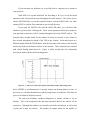
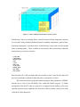
with vehicle heating points however. Figure A below should show the relationship
between the nodes and the vehicle heating points.
Figure A: A TPS cross-section, showing the relationship of nodes and heating points
Since SODDIT is one-dimensional, it can only analyze one heating point at a time. It
does however, calculate the thicknesses and the temperatures at each node. This data can
prove to be helpful if analyzed correctly.
The inner-wall boundary condition temperature is another variable to be set
initially. This is the temperature that the inner-structural shell of the vehicle will be
exposed to. Although this number is not actually used in the calculations, it still is used
in plots and in data for analysis. The number of outputs stands for the number of
calculations to be made by SODDIT over a period of time. Fifty is an appropriate
amount. The Titles are simply notes that appear in the SODDIT output file types; ‘out’
and ‘plt.’ The block 4 data was included to give the user an opportunity to analyze not a
flat plate but a sphere instead. For more information on this, consult the SODDIT User’s
Manual. The current default settings are set for a flat plate assumption.
With these initial figures set and the MAPT.m file saved, MAPT is now equipped
to run adequately. Typing ‘MAPT’ in the Exceed generated MATLAB window will run
the program. At first, you will be given the option to choose between three studies; the
Materials Study, the Thickness Study or the Comprehensive Study. The Materials Study
would be the first option to select.
After clicking on the button, you will notice that the required inputs are all located
on the left side of the screen as is the case for all of the MAPT studies. By selecting the
first material of each combination to be an ablator and then hitting the ‘EXECUTE
ANALYSIS’ button, you will see several comparison plots. The first is a plot of the
surface temperature history for both material combinations. The temperatures level off
because as the ablator ablates away, the surface temperature remains constant. This is
characteristic of an ablator. The second plot shows a comparison of the temperatures at
the middle boundary of the material combinations. The third plot shows the temperatures
at the inner-layer of the TPS. This is the most important plot to take notice of as these
temperatures are the ones that are exposed to the actual vehicle. It should be desired to
keep the inner-layer temperatures below the set boundary condition temperature. Lastly,
the fourth plot shows the ablation depths of the materials, or how much the materials
ablated away. The principle in selecting a good material is to choose one that is lightest
in weight, ablates away at the slowest rate and best insulates the inner structure.
Seen below the plots is a text window that outputs actual data; the maximum
inner-layer temperatures and the maximum ablation depths. All of the provided data
should suffice for comparing any two materials.
To change the material being the analyzed, you may type in the designated boxes
any material name found within the Materials folder in the overall folder. If a new
material is wished to analyzed, the proper material file must be composed. This can be
accomplished by referring to the SODDIT User’s Manual and learning about the
specifications required to write a material file. All material files must be saved within the
Materials folder talked about previously.
To change a material thickness, simply enter in a different value in the respective
text box. However, in the Materials Study, it is important to keep as many variables the
same as possible between different combinations. This study is to determine an optimal
material only, not optimum thicknesses.
If a material is an ablator, make sure that you select the ablator button lying below
it. If you do not, an error might result such as the one seen below:
insufficient data on density record...
...
In the middle is a space to enter the name of the heating file to be used. The
purpose of the heating file is discussed at length within the Team-Daedalus Fall 2005
final report. If a different heating file is used, it is important to note that the actual file
must be located within the overall folder, but NOT in the Materials folder. That folder is
for material files only.
The next input, the maximum analysis time, is a critical value that needs attention.
Because SODDIT cannot analyze any data after the actual vehicle begins radiating heat
away from itself, the SODDIT data ‘blows up,’ or becomes non-meaningful. Therefore,
since an updated version of SODDIT has yet to be made available, every heating file can
only be analyzed up to a certain time; when the heat flux becomes negative. At this
point, the ablation will stop but current research shows that a mild increase in inner-layer
temperature will occur after the SODDIT data turns poor.
More research may be
undertaken in the future surrounding this fact. Since no meaningful analysis can be
performed by MAPT without a maximum analysis time, this temporal point must be
found. This can be accomplished easily within the Materials Study. Simply enter the
name of the heating file-in-question in the proper place. Then set the maximum time to
be the full time of the heating file itself. This number can be found by opening the
heating file with the MATLAB editor and scrolling to the very bottom. On the far left
should be the largest time value. Once this number has been entered, select the ‘I wish to
perform an In-Depth Investigation for Material Combination X at heating point Z’ button.
Fill in 1 or 2 for X and set Z to be the number of one of your columns in the heating file
(as these represent the data for a specific vehicle heating point). Normally, this selected
option can give the MAPT user a very complete understanding of everything that is
occurring at the indicated heating point. The option produces plots displaying nodal
temperature and thickness histories at that heating point. When used to determine the
maximum analysis time however, the resulting plots will look much different than they
would normally appear and they are all characteristic of the poor data caused by a
maximum analysis time that was too large. Examples of such plots can be seen below as
Figures B through C. It is further recommended for the reader to select the ‘I wish to
perform an In-Depth Investigation for Material Combination X at heating point Z’ option
under the default values in order to compare good plots from bad plots. It is hoped that
this will help the user to know when too large of a maximum analysis time is being used.
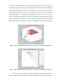
Figure B: Upset 3-D nodal thickness history plot as a result of a too large maximum analysis time
Figure C: Upset 2-D nodal thickness history plot as a result of a too large maximum analysis time
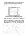
Figures B and C above show the results of indicating a maximum analysis time
that was too large. When SODDIT analyzes the heating file past this time, the data then
tells SODDIT that negative heat flux is occurring (which it very well may be). SODDIT
however cannot handle this and the outputted data ‘blows up,’ characterized by the plots
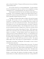
above. In finding an appropriate maximum analysis time, one must manually zoom in on
the plot of the 2-D Nodal Thickness History where the upset data starts to occur. Figures
D through H give a great depiction of this zooming-in process.
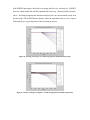
Figure D: Zooming in on Figure C to find an appropriate maximum analysis time
Figure E: Further zooming in on Figure C to find an appropriate maximum analysis time
Figure F: Further zooming in on Figure C to find an appropriate maximum analysis time
Figure G: Further zooming in on Figure C to find an appropriate maximum analysis time
Figure H: Narrowing in on the location of an appropriate maximum analysis time
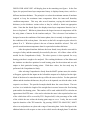
In Figure H, after zooming in on the disastrous ‘apex,’ an arrow can be seen that points to
the area that the user should aim for. The arrow indicates the time right before the
SODDIT data ‘blew up.’ This is the location of an appropriate maximum analysis time.
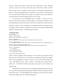
Further zooming in on this point results in Figure I below.
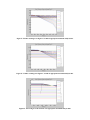
Figure I: An appropriate maximum analysis time has been found as the arrow indicates
The arrow in Figure I shows the time right before the SODDIT data turns poor. This is
an appropriate maximum analysis time. However, it still must be noted that even this
time may be slightly too large for analysis. If resulting official analysis plots later on
show small discrepancies toward the end of the analysis time, most likely the maximum
analysis time should be reduced still. Usually however, these reductions shouldn’t have
to be more than a second.
Once the maximum analysis time has been found, it may be used for the particular
heating file in question. Thankfully, this process of locating the maximum analysis time
only needs to be done once for each heating file used. If a new heating file will be used
in the future, whether within the Materials Study or any of the other two Studies of
MAPT, a new maximum analysis time will need to be found for that heating file.
Elaborating on the In-Depth Investigation, it can prove more useful than just
solving for the blow-out time. It provides much more meaningful plots which can only
be displayed for one heating point, one thickness and one material combination at a time.
This investigation actually creates plots from a single field in the structural array
Data_Collect, and they can prove quit useful in determining TPS behavior at a specific
point or with specific conditions. This process will become more clear as you familiarize
yourself with Data_Collect.
Also an option on the GUI, are the plot-disengagements. The plots within the
GUI can be disconnected for further ease and this can be accomplished by selecting
‘Disengage Plot (X,Y).’ By disengaging the plots, they can be saved for later use.
After the optimal materials have been chosen, the Thickness Study of MAPT may
be undertaken. This is accomplished by exiting out of the Materials Study GUI and retyping MAPT into the Exceed provided MATLAB window. The option menu will come
up once again and the Thickness Study may be selected.
Accordingly, the Thickness Study window will appear, with room for the outputs
on the right, and the inputs on the left.
By pressing ‘EXECUTE ABLATOR
ANALYSIS,’ an example iteration will be run through and the first two figures will
produce data as well as the text box below the four plots. The first figure shows how
much ablation will occur at each indicated heating point, for the planet X heating file
used and for the initial ablator thickness. The second figure shows the same, except it
provides the ablation for the planet Y heating file used. In both cases, the ablator selected
is indicated in the text box marked ‘Ablator Material File Name.’ MAPT displays these
ablation values at the bottom of the screen, adds them together and then adds a safety
margin as was indicated.
The initial thickness entered was not important but was
required to measure the amount of ablation that would occur. It is also important to note
that MAPT produced the preceding for the range of heating points that was indicated.
The indicated range of heating points must be in straight line along the surface of the
vehicle. If two lines exist, then MAPT must used once for each line. The summed
ablation depths with the safety margin are the optimal thicknesses, at the indicated
heating points, for the ablator. Recording these values manually is a must, as the user
will reference them at other times.
The Insulator Analysis part of the Thickness Study is the next task. The selected
insulator name is entered in the respective text box, as is also the first heating point to be
analyzed. In the text box for the ‘Ablator Thickness at Heating Point (m),’ enter in the
optimized ablator thickness at that heating point, previously found. This number comes
straight from the collected data from the Ablator Analysis part. Next the initial insulator
thickness is entered along with minimum and maximum percentages of the initial
insulator thickness to be added or subtracted from the initial value. Pressing ‘EXECUTE
INSULATOR ANALYSIS’ will display plots in the remaining two figures. In the first
figure, the projected inner-layer temperature history is displayed many times, each for a
different insulator thickness. The principle is to select the minimum amount of insulator
required to keep the maximum inner temperature below the inner-wall boundary
condition temperature. This may take several iterations; varying the initial insulator
thickness (or the thickness variant values as they be called) to obtain an appropriate
value. Note that the fourth figure also displays inner-layer temperature histories, but it
does so for planet Y. Whichever planet shows the largest increases in temperature will be
the only planet of interest for the insulator analysis. This is because if an insulator is
designed to meet the conditions of the hottest planet, then it certainly is designed to meet
the conditions of the coolest planet. Also notice on the left is an option to print values for
planets X or Y. Whichever planet is the one of interest should be selected. This will
provide actual maximum temperature data for a particular insulator thickness.
After the optimal insulator thickness has been found, it may then be corrected for
a margin of safety and then manually be recorded by the user. All of these values will be
needed for the Comprehensive Study. The above process is then repeated for every
heating point that is sought to be analyzed. The resulting thicknesses of the ablator and
the insulator are therefore optimized at each heating point for the mission and are each
unique to their particular heating points. With these values, the last study may be
performed: the Comprehensive Study.
After selecting Comprehensive Study from the MAPT options menu, the window
will appear, again with the inputs on the left and the outputs to be displayed on the right.
Much of the data to be entered near the top will be the same as before. For the optimized
ablator and the insulator thicknesses, they all are to be inputted, one after the other, in the
respective text boxes. The provided example should show the correct format. The next
text box is to include the length of the straight line in meters between the first heating
point and the last heating point. This number will be used within MAPT to calculate an
approximate final TPS mass. Also used to calculate the mass is the required surface area
of the vehicle that will be covered by TPS. Required still, is the percentage of the width
of the vehicle the user wishes the heating point range to cover. Lastly, the user would
input the densities of the TPS materials. By pressing ‘EXECUTE ANALYSIS,’ MAPT
takes over and produces two plots and a range of interesting data. In the first figure is the
ablation behavior with respect to time as the vehicle travels through planet X and then
through Planet Y. The dark line in the center of the ablator indicates where the ablation
left off as it exits planet X’s atmosphere and picks up in planet Y’s atmosphere. The
amount of ablative material left after the second planet can be seen, resting on the
insulator. The orange line at the bottom indicates the ceiling of the insulator. The second
figure shows the inner temperature of the vehicle with respect to time as the vehicle
travels through planet X and then planet Y. In the second figure, the inner temperatures
should never reach above the boundary condition as the insulator has been optimized and
in the first figure, the ablation should never sink below the safety margin.
Aside from the data outputted which will be left for the reader to explore, the next
outputs of major interest are the TPS masses. By using a polynomial fitting technique
with the inputted thicknesses and computational integration, a final TPS mass for the
ablator and the insulator can be solved for. The exact method may be explored within the
Comprehensive_GUI.m file. It is important to note that unless the percent-of-surface
covered by the heating point span was 100%, the displayed masses are not all inclusive.
If two lines of heating points exist, for example one line (possibly down the center of the
vehicle) may be assumed to serve as 33% of the vehicle, while the other line (possibly
between the center and the side) may serve as 33% on each side but 67% would be used
to account for that line on each side of the vehicle.
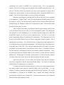
If the user selects the ‘Create Plot of TPS Material Shapes along Heating Point
Span’ button, a plot will result of the actual shapes of the TPS materials, one laying on
top of the other.
Lastly, the Comprehensive Study includes the option to create movies of plots 1
and 2 with respect to time. If one of these options is selected, be prepared to wait for
around one hundred frames to display and save. Each frame takes about 2 seconds to
display and save. Also, be careful in this process not place anything in front of the
recording screen or the object itself will be recorded also. It is furthermore important not
to manually close the recording figure when you think that the last frame has completed.
This could negatively affect the movie. When the recording process is complete, the
frames will close themselves.
Whether it is wished to play a user-created movie or the initial movies first
provided when the MAPT program package was downloaded, the process is simple.
There is no need to press an ‘EXECUTE ANALYSIS’ button. Simply press the ‘Play
Movie’ button at the top of the Comprehensive Study GUI. It should be found just above
the plots. Before pressing play, the user must select which movie to play. When the
selection is made, the user may sit back and enjoy the animation created by MAPT.
What is being viewed is a composite of many frames, each showing the nodal-thickness
history over an entire heating point span. Each frame was recorded at a different moment
in time and when MATLAB puts them together, an animation of the actual ablation or
temperature history across the heating point span can be viewed.
Several errors may occur throughout the use of MAPT. If one does occur, recheck the entered data to make sure that the ablator is not ablating completely away or
that something wasn’t entered incorrectly. MAPT has run many times and has proven its
capability. If there is an error, something else other than the MAPT code must be wrong.
If a problem cannot be found, try closing out the window, Exceed and the UNIX platform
and start it all up once again. If the following error results:
Creating "soddit_script.exe"
??? Error using ==> fprintf
Invalid file identifier -1.
Error in ==> create_script at 40
fprintf(fp,['export PATH=$PATH:' soddit_path ' \n']);
Error in ==> mysoddit at 69
[success, actual_file_name] = create_script(file_name, soddit_path, soddit_exe, current_directory);
Error in ==> soddit_between at 25
[T_max(lcv),Time_max(lcv)] =mysoddit(scale(lcv),number_of_materials,materials(:,mcv),opt_struct,block4,header,t_init);
Error in ==> Materials_GUI>pushbutton1_Callback at 180
[T_max,Time_max] = soddit_between(sweep,number_of_materials,materials,opt_struct,block4,header,t_init);
Error in ==> gui_mainfcn at 75
feval(varargin{:});
Error in ==> Materials_GUI at 56
gui_mainfcn(gui_State, varargin{:});
??? Error while evaluating uicontrol Callback.
Then try closing everything out and restarting. If an error shows up saying that the disk
quota has been exceeded, then your tomb file has been filled and needs to be emptied.
This can be accomplished by exiting out of Exceed. Then on the UNIX platform, type
‘unrm.’ This should give you a ‘unrm>>’ prompt. At this point, type in ‘purge [space] *’
and hit enter. The tomb file will then empty and you may press ‘exit’ to return to your
normal prompt.
Hopefully this document will provide enough background information to give the
user a good start with using and interpreting the McDaniel Analysis Program for Thermal
Protection Systems. If an understanding of the methodology of the code itself is desired,
then the proceeding section was written for that purpose.
PART II: ENCODING METHODOLOGY OF M.A.P.T.
The author is hopeful that the internal comments within the MATLAB scripts of
MAPT will be of some use to the reader in trying to understand the methodology of the
files. For MAPT, three major MATLAB scripts were composed; Materials_GUI.m,
Thickness_GUI.m and Comprehensive_GUI.m. Within each of these as is discussed in
the TPS section of the Team-Daedalus report, is the execution of soddit_between.m. This
is the gateway file which executes SODDIT itself, but it also serves as the means to
create the structural array Data_Collect, used to store and collect the SODDIT data. An
investigation of the MAPT files would should show that soddit_between.m is called on
occasion and is done so strictly to run SODDIT and to store data within Data_Collect.
As can be seen in soddit_between.m, mysoddit.m (which is the file responsible for
compiling the SODDIT input files and reading the SODDIT output files) can be executed
for a certain amount of material thicknesses, heating points or material combinations.
Materials_GUI.m uses soddit_between.m to execute mysoddit.m for a certain number of
material combinations over a single heating point. Thickness_GUI.m, in the Ablator
Analysis, uses soddit_between.m to execute mysoddit.m over a range of heating points
for a constant material thickness and for a single material combination.
Further,
Thickness_GUI.m within the Insulator Analysis, uses soddit_between.m to execute
mysoddit.m for a variable value of material thicknesses, but does so for a single material
combination and for a single heating point.
Lastly, Comprehensive_GUI.m uses
soddit_between.m to execute mysoddit.m for a range of heating points but only for a
single material combination and for a constant material thickness (even though
soddit_between.m is executed with a different material thicknesses each time).
For all of these changing parameters, the structural array Data_Collect was
created to store all of the various types of data. Although it has three-dimensional
capability, only the two facing ‘planes’ are needed within MAPT. A diagram of the
structural array Data_Collect can be seen below as Figure J.
Figure J: Artists rendition of structural array Data_Collect
Within Data_Collect are multiple fields, each field stored with the temperature histories
of every node, along with their thickness histories, boundary temperatures, spans of time,
maximum temperatures, maximum times, initial thickness values and even the heating
index (or heating point). These variables are mirrored by their actual names within the
structural array as can be seen below.
T_all_nodes
T_boundaries
Thickness_hist
Time
T_max
Time_max
sweep_value
heating_point
mat_names
mat_orthick
Each field has all of the preceding data stored within it and is used by the other files
previously mentioned to obtain the data and plots reviewed above in Part I.
This concludes the basic principles behind storing the data outputted by SODDIT,
and the use of some of the old Heckler files within the MAPT program. If further
descriptions of the MAPT codes are required, it is suggested by the author to refer to the
encoded comments made within the files themselves and to perform a line by line study
of the MAPT files themselves.