Download LaDiCaoz and LiDARimager–MATLAB GUIs for LiDAR data

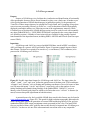
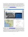
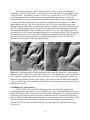
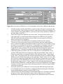
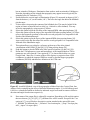
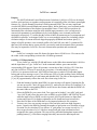
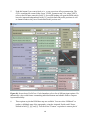
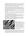
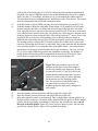
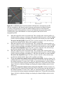
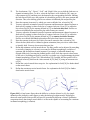
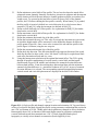
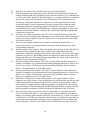
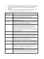
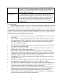
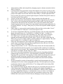
Supplementary material to “LaDiCaoz and LiDARimager–MATLAB GUIs for
LiDAR data handling and lateral displacement measurement”
Olaf Zielke1*, J Ramon Arrowsmith1
1
School of Earth and Space Exploration, Arizona State University, Tempe, AZ, 85287, USA.
* To whom correspondence should be addressed: E-mail: [email protected]
Table of contents
LiDARimager–manual…….……………………………………………………………………...2
Purpose..…………………………………………………………………………………...2
Input data………………………………………………………………………………….2
LiDARimagerGUI functionality………………………………………………………….4
Worked example………………………………………………………….……………….7
LaDiCaoz –manual .………...…………………………………………………………………….9
Purpose……………………………………………………………………………………9
Input data………………………………………………………………………………….9
LaDiCaoz GUI functionality………………………………………………...…………...10
Worked example………………………………………………………………………....18
1
LiDARimagermanual
Purpose
Purpose of LiDARimageris to facilitate the visualization and identification of horizontally
offset geomorphic features (such as fluvial channels) as they cross a fault zone. It further serves
a) the quick generation of LiDAR-based imagery in publication quality, b) the generation of
*.kmz files of these images that may be uploaded to Google Earth, and c) cropping of large data
sets to increase processing efficiency in LaDiCaoz –a tool to determine offsets of horizontally
displaced geomorphic markers (see following section of the supplementary material). While
LiDARimagerwas developed for LiDAR data processing it may be used to work with essentially
any other gridded DEM (e.g., USGS DEM, SRTM) that is presented in the correct input format
(see following section). A number of conversion tools are available for the possibly required
transformation of the input data format, including ESRI’s ARCGIS and FWtools (based on open
source GDAL).
Input data
LiDARimagerand LaDiCaoz can read gridded DEM data, stored in ESRI’s non-binary
ARC grid format or a generic ASCII grid format. Figure S1 presents example layouts of these
data formats. The data are required to be stored in x-y-z coordinates (UTM coordinates) to be
processed in LiDARimageror LaDiCaoz.
Figure S1. Possible input data formats for LiDARimagerand LaDiCaoz. The input values for
“north”, “south”, “east”, and “west” define the spatial extent of the data set in UTM coordinates.
“xllcorner” and “yllcorner” refer to Easting and Northing coordinates of lower left corner of data
set (SW-most data point).” (n)cols” and “(n)rows” respectively refer to the number of rows
(along Northing) and columns (along Easting) of the gridded DEM. “NoDATA” serves as
dummy value to identify grid points for which no elevation data exist. “cell size” is distance (in
meter) between data points (equidistant in both directions).
A potential source for freely available LiDAR data, stored in this format, may be found at
www.opentopography.org (Figure S2). This portal for high resolution topographic data and tools
allows among other options the generation of custom DEM and the download of 0.5m grid size
standardized DEM (IDW return or minimum return), presented in 1km2 tiles. The latter DEM
tiles are provided as binary ARC-grid files that can not directly be imported into LiDARimageror
LaDiCaoz. You have to use one of the aforementioned conversion tools or any comparable
2
software package that is capable of converting binary ARC to ASCII grids. When possible, we
recommend generation of custom DEM. During this process you may choose interpolation
method, product download format, grid resolution, and search radius (Figure S2). These options
may be of particular importance when investigating areas with dense vegetation cover, requiring
adjustment of grid resolution and interpolation method. For further instructions on how to
acquire a custom DEM from www.opentopography.org and how to set the respective options we
want to refer the reader to the help section of this web portal.
Figure S2. Screen shots of www.opentopography.org web portal for freely available LiDAR
data and tools. A) Main page of the site, presenting different download options including “Point
Cloud Data and Custom DEMs” and “Standard DEMs”. B) Spatial extent of “B4” LiDAR data
set along the southern San Andreas Fault and San Jacinto Fault (in yellow). Zoom to region of
interest and interactively select area for which data are to be downloaded. C) Options of custom
DEM generation, including interpolation method, grid size, and search radius. Consult the help
provided on this site for additional explanation of respective options.
3
The maximum DEM size that LiDARimagerand LaDiCaoz can process depends on
availability of memory. DEM with <107 grid points work well in both GUIs for computers with
>2Gb of memory. LiDARimagerfeatures a “quick view” to load only every 2nd to 5th line and
row of the imported data set, allowing to process significantly larger data sets. If used, the
imported DEM have a lower spatial resolution than the original data set. This resolution however
is usually sufficient to depict fault trace and offset geomorphic features (Figure S3A). When
output data are saved as *.asc file in LiDARviewer, the GUI will use the spatial extent of the
hillshade window (Figure S3A, inset B) to crop and save a smaller section of the DEM. For that
the GUI opens the original data set and only imports data points within the spatial extent of the
aforementioned hillshade window and then saves them to a *.asc file. Thus, using “quick view”
does not result in a loss of data resolution when saved to *.asc format (Figure S3B). We typically
use LiDARimagerto visualize large tiles of LiDAR-generated DEM and to identify fault trace
and offset features. We then crop and save smaller sections of this data set for each offset
features that was identified within the imported DEM.
Figure S3. A) Hillshade plot of LiDAR-generated DEM, using the “quick-view” option during
data import (here “3-Quick” was used; that is only every 3rd row and column of the original data
set is imported). Original grid size is 0.25m, grid size in A is 0.75m. Topographic features are
sufficiently represented to identify offset features. B) Example for an extracted DEM (using the
*.asc save option) that was re-imported into LiDARimager(without quick-view option) to present
full data set resolution.
LiDARimagerGUI functionality
To use LiDARviewer, start MATLAB and browse to the folder that contains both,
LiDARimagerand the input data set. Type “LiDARviewer” in the command window, press enter
and the GUI opens. Figure S4 presents a screen shot of the LiDARimagerGUI. Note that only one
LiDARimagerGUI may be open at each time--if more than one GUI is open MATLAB will not
know to which GUI individual inputs belong and an error messages occur. Close all but one GUI
to fix this problem. In the following we will describe the functionality of each button and
editable field. The order of descriptions (from [1] to [18]) reflects the work flow when using
LiDARviewer.
4
Figure S4. Screen shot of LiDARviewer. Circled numbers refer to list of different input options.
1.
2.
3.
4.
5.
6.
7.
Push this button to load the input DEM. An error message will appear if opening the file
was not successful. Check for typos in field [3], make sure the correct file extension [2] is
chosen, that the corresponding DEM is in the correct data format, and that the DEM is in
the same folder as the GUI.
Select the file type of the DEM file you want to load. Two types can be loaded: *.asc
(ARC grid) and *.asc (ASCII grid) where the prior refers to DEM, saved in ESRI’s
ARCGIS ASCII-grid while the latter refers to DEM, saved in a generic ASCII-grid
format (see Figure S1 for examples).
Enter the file name of the DEM that is to be imported without its file extension.
You may use a box-car moving average to filter out holes and some high-frequency
(noise-) signal in the DEM by entering the number of grid points over which the average
elevation is to be calculated. If you choose “0” grid points, no averaging is used; for “3”,
the average elevation of a 3x3 wide box around each grid point is determined and
assigned to the center grid point. This step will be performed during data import (after
pushing button [1]). Note that averaging noticeably increases the data import time.
Choose this option to load only every 2nd to 5th line and row of the DEM that is to be
imported. This option allows processing large, high-resolution DEM. When “None” is
chosen, the whole data set is imported. Select a value other than “None” if data import
(using “None”) was unsuccessful and if MATLAB indicated a lack of available memory.
When you use the Quick draw option (a value other than “None”) and save to *.asc, then
the GUI will re-import the original DEM (at full resolution) and select the values within
the spatial extent of the hillshade plot to save them to the output file. If you have not used
the Quick draw option (value is “None”) then the GUI will export the portion of the
already initialized DEM that is within the spatial extent of the hillshade plot. That means,
if you have used moving average (while not using Quick draw), then the exported DEM
will be the averaged one.
Select this option to plot a hillshade view of the imported DEM when pressing button
[14]. Hillshade plots may be adjusted by changing the illumination angle (azimuth and
zenith) and illumination contrast (z-factor; fields [7]-[9]).
Azimuth defines the horizontal angle of illumination (Figure S5). The angle is measured
in degrees (0-360°) from south and in counter-clockwise direction. For example:
illumination from south to north has an azimuth of zero. Illumination from east to west
5
8.
9.
10.
11.
12.
13.
14.
15.
has an azimuth of 90degrees, illumination from north to south an azimuth of 180degrees.
Note that, depending on the azimuth the topography may appear inverted (typically for
azimuths below 90° and above 270°).
Zenith defines the vertical angle of illumination (Figure S5) measured in degrees (0-90°)
from the horizon ( =0°) to the zenith (=90°). The lower the angle the darker the hillshade
plot becomes.
Z-factor allows increasing the contrast of the hillshade plot. This may be helpful if the
region or feature of interest has low relief (e.g., fault trace, offset channel). You may
invert the topography by using negative Z-factors.
Select this option to plot the elevation of the imported DEM when pressing button [14].
Select this option to plot the slope of the imported DEM when pressing button [14]. Slope
refers to the steepness (gradient) of the surface at each grid point. It is comparable to the
Zenith of the illumination angle.
Select this option to plot the aspect of the imported DEM when pressing button [14].
Aspect refers to the dip direction of the surface at each grid point. It is comparable to the
Azimuth of the illumination angle.
This option allows you to display a reference grid on top of the afore plotted
visualizations of the DEM ([6] and [10]-[12]) when pressing button [14].
Push this button to plot the DEM in the afore specified options ([6] and [10]-[12]).
Define the UTM parameters (zone and hemisphere) of the imported data set. These
parameters are used when the *.kmz option in [17] is chosen which allows to create
Google Earth *.kmz files. Creation of these files requires re-projection from UTM
coordinates (in which the imported DEM are stored) to decimal degree geographic
coordinates (WGS84) and therefore definition of the UTM zone.
Figure S5. A and B) Hillshade view of the topography at Bidart Fan in the Carrizo Plain, San
Andreas Fault, exemplifying the effect of different illumination angles. C) in LiDARimagerand
LaDiCaoz, azimuth and zenith are defined as indicated: angle from south in counter-clockwise
direction and angle from horizon respectively.
16.
Enter name of the output file(s) without file extension. Depending on file and plot option
that was chosen, ([6], [10]-[12], [17]) different files will be created. Except for the *.asc
option in [17], saved files have descriptive section attached to the entered file name
(“_Hillshad” for hillshade plot; “_Elevation” for elevation plot; “_Slope” for slope plot;
and “_Aspect” for aspect plot).
6
17.
18.
Select file type option for output file. You may save output as *.jpeg, *.kmz, and *.asc
file. The prior two options generate output files with of the plotted DEM images ([6],
[10]-[12]). The third option is using the spatial extent of the current zoom of the hillshade
plot to save a corresponding subsection of the DEM to a *.asc file with name defined in
[16]. We recommend using this data set cropping option to increase computational
efficiency when using the output data set (*.asc file) in LaDiCaoz. See explanation for
field [5] and Figure S3 for additional information when saving to *.asc file.
Save output data set using name and file type, defined in fields [16] and [17]. A message
dialog box appears after the selected files were successfully saved. Only data that are
currently active (plotted) will be saved to file. See explanation for field [5] for additional
information when saving to *.asc file.
Worked Example
A.
Start LiDARimagerin MATLAB prompt and make sure that DEM data set is located in
the same folder.
B.
Enter file name in field [3], file extension in field [2] and load options. Here we use a
sample data set called “Sample1.asc” that is saved in ARC grid. Leave option [4] and [5]
untouched and press [1] to load the data. Close message dialog after in informed of
successfully loading the DEM.
C.
Press button [14]. A hillshade plot that uses the illumination parameters, specified in [7][9] is plotted. Close the plot.
D.
Change [7] to 220, [8] to 35, and leave [9] at 1. Then press button [14] again to create
hillshade plot with new illumination parameters.
E.
Repeat steps C and D (with varying values for [7]-[9]) until you have gained good
understanding of topography, fault trace and offset features.
F.
Change [4] to value of 5 (thus using 5x5 moving average) and press button [1] again to
reinitialize the imported data set. Note the increase in loading time.
G.
Press button [14] to see effect of moving average. Repeat step F and G to see effect of
varying box-car sizes.
H.
Set [4] to zero again and change [5] to “2-Quick” which loads only every 2nd row and
column of the imported data set (“3-Quick” loads every third row and column and so
forth). Then press [1] again to reinitialize the data set.
I.
Press button [14] to see the effect of Quick-draw. Repeat step H and I to see effect of
varying the grid size resolution.
J.
Set [4] to 3 and [5] to “None” and press button [1].
K.
Select fields [10] to [12] and press [14] to plot all views: hillshade, elevation, slope, and
aspect image. Investigate respective images to see how respective geomorphic features
are expressed in different view options.
L.
Enter output file name in field [16] e.g., “Sample1a”, select *.jpeg option in [17] and
press button [18]. Only images of currently open figures will be printed to file (i.e.,
saved).
M.
Enter output file name in field [16] e.g., “Sample1a”, select *.kmz option in [17] and
press button [18]. Only images of currently open figures will be printed to file (i.e.,
saved). Open respective *.kmz files in Google Earth to overlay hillshade plots etc. with
Google Earth imagery. You may recognize the slight mismatch between *.kmz and basemap imagery, an issue we are currently working on.
7
N.
O.
P.
Enter output file name in field [16] e.g., “Sample1_cut”, select *.asc option in [17] and
press button [18]. Before that zoom the hillshade map to an area similar to the one
presented in Figure S3B. Saving to *.asc will then create an ARC-grid DEM with the
spatial extent of the data presented in the hillshade view.
Change input file name in field [3] to the name used during step N in field [16] (e.g.,
“Sample1_cut”), set [4] to zero, and press button [1]. This will load the new (and
cropped) DEM. You may use this step if you have imported a large DEM (using Quick
draw) and think to have identified an offset feature. You may crop and save to the
surrounding of this feature (creating a *.asc grid file ([16]-[18]) and then load it again
without using Quick draw to increase the spatial resolution.
Otherwise, you may use the “Sample1_cut.asc” file for further processing and offset
measurement in LaDiCaoz.
8
LaDiCaoz -manual
Purpose
The MATLAB-based Lateral Displacement Calculator (LaDiCaoz) GUI was developed
to allow quick and easy-to-reproduce measurements of tectonically offset, sub-linear geomorphic
features (e.g., fluvial channels) based on LiDAR-generated DEM. The user may import and
visualize the DEM (create hillshade and contour plots), define fault trace, cross-sectional profile
position, and orientation of the displaced geomorphic feature. Then LaDiCaoz performs an
automated offset calculation using the afore defined input parameters, who’s results may be
assessed sub-quantitatively and qualitatively by back-slipping cross-sectional profiles and
topography respectively. To ensure that the results of these measurements are as transparent and
repeatable as possible, we designed LaDiCaoz to create multiple output files, including a) highresolution images of current and back-slipped topography (hillshade and contour plots), b)
images of profile position, cross-sectional profile relief, and GoF plot, and C) a parameter file
that stores all relevant data to repeat (reload) a previously made measurement (those parameter
files may be imported to LaDiCaoz for exact measurement repetition and assessment).
Input data
LaDiCaoz is using the same file format for input data as LiDARviewer. We want to refer
the reader to the corresponding section in the LiDARimagermanual.
LaDiCaoz GUI functionality
To use LaDiCaoz, start MATLAB and browse to the folder that contains both, LaDiCaoz
and the input data set. Type “LaDiCaoz” in the command window, press enter and the
corresponding GUI appears. Figure S6 presents a screen shot of the LaDiCaoz GUI. Note that
only one LaDiCaoz GUI may be open at any given time--if an individual GUI (such as
LaDiCaoz) is open more than once, MATLAB will not know to which GUI individual inputs
belong and an error messages occur. Close all but one GUI to fix this problem. In the following
we will describe functionality of each button and editable field. The order of descriptions (from
[1] to [49]) approximately reflects the work flow when using LaDiCaoz.
1.
2.
3.
4.
Push this button to load the input DEM. An error message will appear if opening the file
was not successful. Check for typos in field [3], make sure the correct file extension [2] is
chosen, that the corresponding DEM is in the correct data format, and that the DEM is in
the same folder as the GUI.
Select the DEM file you want to load. Two types can be loaded: *.asc (ARC grid) and
*.asc (ASCII grid) where the prior refers to DEM, saved in ESRI’s ARCGIS ASCII-grid
while the latter refers to DEM, saved in a generic ASCII-grid format (see Input Data
section and Figure S1 for further explanation on file format and conversion tools).
Enter the file name of the DEM that is to be imported without its file extension.
You may use a box-car moving average to filter out holes and some high-frequency
(noise-) signal in the DEM by entering the number of grid points over which the average
elevation is to be calculated. If you choose “0” grid points, no average is used; for “3”,
the average elevation of a 3x3 wide box around each grid point is determined and
assigned to the center grid point. This step will be performed during data import (after
pushing button [1]). Note that averaging noticeably increases the data import time.
9
5.
Push this button if you want to look at i.e., re-run a previous offset reconstruction. The
GUI is searching the current folder for an “XXXX_parameter.mat” file, where XXXX
refers to the file name entered in field [3]. Successful loading will open the DEM (which
has to be imported independently before [1]) and plot fault and profile positions as well
as channel trends as they have been defined in the previous run.
Figure S6. Screen shot of LaDiCaoz. Circled numbers refer to list of different input options. We
thematically color-coded frames surrounding individual buttons and editable fields to improve
layout and usability.
6.
Three options to plot the DEM base map are available. You can select “Hillshade” to
produce a hillshade map of the topography, using the Azimuth, Zenith, and Z-factor,
defined in field [7], [8], and [9]. You can select “Contour” to produce a contour plot of
10
7.
8.
9.
10.
11.
the topography, using the number of contours defined in [12]. The third option is to select
both, hillshade and contour. In this case the hillshade map is overlain by a contour plot
using the contour number defined in [12]. Generally, it is recommend using only
hillshade plots as base maps and not contour plots. Contour plots are recommended for
evaluation of the channel reconstruction (during back-slipping).
Azimuth defines the horizontal angle of illumination (Figure S5). The angle is measured
in degrees (0-360°) from south and in counter-clockwise direction. For example:
illumination from south to north has an azimuth of zero. Illumination from east to west
has an azimuth of 90degrees, illumination from north to south an azimuth of 180degrees.
Note that, depending on the azimuth the topography may appear inverted (typically for
azimuths below 90° and above 270°).
Zenith defines the vertical angle of illumination (Figure S5) measured in degrees (0-90°)
from the horizon (=0°) to the zenith (=90°). The lower the angle the darker the hillshade
plot becomes.
Z-factor allows increasing the contrast of the hillshade plot. This may be helpful if the
region or feature of interest has low relief (e.g., fault trace, offset channel). You may
invert the topography by using negative Z-factors.
When the DEM was successfully loaded by pushing button [1], the minimum elevation
value of the input DEM is plotted here. During back-slipping [41] this value [10] is
adjusted to the minimum value that is displayed within the current zoom (hillshade
figure, Figure S7). Also see explanation of field [12].
When the DEM was successfully loaded by pushing button [1], the maximum elevation
value of the input DEM is plotted here. During back-slipping [41] this value [11] is
adjusted to the maximum value that is displayed within the current zoom (hillshade
figure, Figure S7). Also see explanation of field [12].
Figure S7. A) Hillshade view of an
example data set. When using [13] to plot
the DEM, values [10] and [11] are set to be
equal to maximum and minimum elevation
within the imported data set (all of A).
When using [41] to back-slip the DEM
(currently presented in hillshade view), the
values in [10] and [11] are adjusted to
display maximum and minimum elevation
value within the current hillshade zoom
(e.g., in “B”). This procedure is increasing
computational efficiency.
12.
Defines the number of contours plotted. If you make a contour plot of the base map using
[13] (not of back-slipped topography using [41]) the elevation difference is equal to the
maximum and minimum elevations within the imported data set--respective values are
presented in fields [11] and [10]--so that you can determine the contour interval that
corresponds to the contour number: ([11]-[10])/[12] = contour interval. If you make a
11
13.
14.
contour plot for back-slipping [41], LaDiCaoz determines the maximum and minimum
elevation value that is within the current zoom of the hillshade plot (Figure S7), updates
fields [10] and [11] accordingly, and then uses [12] to determine the contour interval.
This procedure decreases computation time and focuses on the offset feature. The contour
interval is displayed in the MATLAB command window.
Push this button to plot the DEM using the afore specified options ([6] and [10]-[12]).
Push this button to define the fault trend. When button [14] is pushed LaDiCaoz opens
the base map plot and allows to define start and end point of the fault trace via mouse
click. Move the mouse to one end of the fault trace and left-click. Then move to the other
end of the fault trace and left-click again. We usually put a ruler onto the computer screen
along the fault trace when tracing the fault. After tracing (after the 2nd mouse-click), fault
and profile line as well as the corresponding cross-sectional profiles are drawn in
hillshade plot and profiles plot respectively (fault in turquoise, profiles in red and blue).
The starting position of the profile (left end in profiles plot) is indicated by a dot in the
base map. Ensure that the fault trace is sufficiently long so that upstream and downstream
cross-sectional profiles are covering the offset geomorphic feature. Also ensure that the
traced fault is at the proper position and has the proper orientation. You may use field
[23] to [28] to adjust fault trace position and orientation accordingly. The number of
profile points is defined by profile length and the increment size in field [36]. Each
profile point is assigned the elevation of the nearest grid point (Figure S8).
Figure S8. Fault (turquoise) as well as red
and blue profile lines across offset channel.
Profiles are parallel to the fault trace; db and
dr (entered in fields [15] and [16]) define the
normal distance between fault trace line and
respective profile. Field [36] allows defining
the increment size (dx) along the profile
line. The elevation of each profile point is
set equal to the elevation of it nearest
neighbor grid point (indicated by triangles in
inset image).
15.
16.
17.
Enter the distance between fault trace and blue profile line (Figure S8).
Enter the distance between fault trace and red profile line (Figure S8).
Blue and red profile can be cut on both ends. This is usually done with one profile (e.g.,
the blue profile) to improve calculation of the optimal offset (the goal is to fit the channel
profiles, not the topography surrounding it). Enter here the amount you want to cut off
the start of the blue profile (Figure S9). Once you have entered a value, the base map
(profile line) and the Profiles figure will be updated accordingly.
12
Figure S9. A) Hillshade plot of an offset channel with fault trace (in turquoise), profile
lines (in red and blue) and channel trend of upstream and downstream channel segment
(in yellow). B) Projected (to account for channel obliquity relative to the fault trace)
topographic profiles. Both profiles have been cut on both ends. Start point of the profile
is indicated by a dot in the hillshade view and corresponds to the left side of the
topographic profile.
18.
19.
20.
21.
22.
Blue and red profile can be cut on both ends. This is usually done with one profile (e.g.,
the blue profile) to improve calculation of the optimal offset (the goal is to fit the channel
profiles, not the topography surrounding it). Enter here the amount you want to cut off
the end of the blue profile (Figure S9). Once you have entered a value, the base map
(profile line) and the Profiles figure will be updated accordingly.
Blue and red profile can be cut on both ends. This is usually done with one profile (e.g.,
the blue profile) to improve calculation of the optimal offset (the goal is to fit the channel
profiles, not the topography surrounding it). Enter here the amount you want to cut off
the start of the red profile (Figure S9). Once you have entered a value, the base map
(profile line) and the Profiles figure will be updated accordingly.
Blue and red profile can be cut on both ends. This is usually done with one profile (e.g.,
the blue profile) to improve calculation of the optimal offset (the goal is to fit the channel
profiles, not the topography surrounding it). Enter here the amount you want to cut off
the end of the red profile (Figure S9). Once you have entered a value, the base map
(profile line) and the Profiles figure will be updated accordingly.
Define the trend of the channel section, cut by the blue profile. Similar to button [14],
pushing button [21] opens the base map figure. Here you can enter start and end point of
the channel trend line via mouse click. After you entered both points, a yellow dashed
line is plotted in the base map plot outlining the channel trace. The profile in the profiles
figure will also be shifted accordingly (accounting for channel obliquity relative to the
fault trace).
Define the trend of the channel section, cut by the red profile. Similar to button [14],
pushing button [22] opens the base map figure. Here you can enter start and end point of
the channel trend line via mouse click. After you entered both points, a yellow dashed
line is plotted in the base map plot outlining the channel trace. The profile in the profiles
figure will also be shifted accordingly (accounting for channel obliquity relative to the
fault trace).
13
23.
24.
25.
26.
27.
28.
29.
30.
31.
The four buttons “Up”, “Down”, “Left”, and “Right” allow you to shift the fault trace or
channel orientation lines. To do so, select the line that is to be shifted in [28], enter an
offset amount in [24] and then press the button for the corresponding direction. Shifting
the fault line will also move the position of red and blue profile by the same amount and
direction. Thus, after shifting, profiles are redrawn in hillshade plot and profiles plot.
Enter the amount (in meters) by which you want to shift the line, selected in [28].
You may adjust the orientation (trend) of upstream and downstream channel segment or
fault trace by rotating it either clockwise or counter-clockwise. Press [25] to rotate the
line selected in [28] by the amount defined in [27] in clockwise direction. Profiles are
redrawn in hillshade plot and profiles plot when features are rotated.
You may adjust the orientation (trend) of upstream and downstream channel segment or
fault trace by rotating it either clockwise or counter-clockwise. Press [25] to rotate the
line selected in [28] by the amount defined in [27] in counter-clockwise direction.
Profiles are redrawn in hillshade plot and profiles plot when features are rotated.
Enter the amount (in degrees) by which you want to rotate the line, selected in [28].
Select the line (fault trace or channel segment orientation) that you wish to either rotate
or laterally shift. You may choose more than one line.
Define the minimum vertical stretch factor. The blue profile can be adjusted by stretching
it vertically (changing its z-factor) to account for different morphologic evolution of
upstream and downstream channel segment. For example, a beheaded channel may
degrade diffusively (lowering the channel profile relief) while the respective head water
is still active. Stretching one profile vertically is a simple way of approximating the initial
channel morphology (Figure S10). When button [39] is pushed, the blue profile will be
stretched iteratively between the values entered in [29] and [31] using an increment size
of [30].
Define the vertical stretch factor step size. See explanation for field [29] for further detail
on the stretch factor.
Define the maximum vertical stretch factor. See explanation for field [29] for further
detail on the stretch factor.
Figure S10. Left and center figure show the diffusive evolution (from t0 to t2) of a simple
channel profile (shifted in center figure to make the thalweg locations match). Right figure
shows an actual profile (blue profile in Figure S9) stretched by different z-factors. Qualitative
comparison shows that using a stretch factor is to first order capable of accounting for variations
in channel morphology (evolution).
14
32.
33.
34.
35.
36.
37.
38.
39.
Define minimum vertical shift of blue profile. The tool was developed to match offset
ephemeral stream channels. Naturally, the thalweg elevation at upstream and downstream
profile location will be different (otherwise channel gradient would be zero and no flow
would occur). To account for that and allow a better fit (lower GoF) of the channel
profiles, the GUI allows shifting the blue profile vertically. When button [39] is pushed,
the blue profile is iteratively shifted in a vertical direction by a value between those
entered in [32] and [34], using the increment size defined in field [33].
Define vertical shift step size of blue profile. See explanation for field [32] for further
detail on the vertical shift.
Define maximum vertical shift of blue profile. See explanation for field [32] for further
detail on the vertical shift.
Define the minimum horizontal slip of the blue profile.
Define the horizontal slip step size. This value is not only the increment size (precision)
in which the displacement will be measured. It also defined the distance dx between
profile points (Figure S8). Once a new value is entered, the red and blue profile in the
profile figure is redrawn, using the new step size.
Define the maximum horizontal slip of the blue profile.
Define back-slip direction. This direction should be the opposite direction of the actual
fault slip direction. In other words, select “left-lateral” back-slip for a right-lateral fault
such as the San Andreas Fault and vice versa.
Using this button starts calculation of the optimal horizontal offset. The GUI is going
through all possible combinations of vertical stretch, vertical shift, and horizontal
displacement (Figure S11B, middle) and calculates the summed elevation difference
between both profiles. From the resulting three-dimensional data cube the minimum
summed elevation difference i.e., maximum Goodness of Fit (GoF, inverse of summed
elevation difference) is selected. The corresponding optimal horizontal displacement,
vertical stretch and vertical displacement are displayed in the MATLAB window.
Figure S11. A) Fault, profile and channel segment location and orientation. B) Top panel shows
overlay of red profile and back-slipped blue profile (using parameter combination that resulted in
max. GoF (see bottom of S11B). Middle panel shows parameters changed in offset calculation.
Bottom panel shows GoF as function of horizontal displacement for parameter combination
(vertical shift and stretch) that contained max. GoF. C) Back-slipped hillshade plot of
topography to visually assess channel reconstruction (back-slipped by 6.0m).
15
40.
41.
42.
43.
44.
45.
46.
47.
48.
Enter the value (in meter) by which the base map will be back-slipped.
Push this button to back-slip the base-map in the direction, defined in field [38] by the
amount defined in field [40]. Depending on the selection in fields [6]-[12] a hillshade plot
or contour plot will be produced. The back-slipped i.e., reconstructed surface may then be
inspected to visually assess the quality of the reconstruction. If reconstruction is not
satisfying it is likely that channel trace, fault trace, or profile position may have been
chosen unfavorably. Note the importance of having a general idea of what the initial
topography and channel morphology might have looked like--the user has to make a
conscious decision on what is considered the pre-earthquake topography, in other words
what part of the profile should be correlated. We recommend using both, hillshade and
contour plots for this step.
LaDiCaoz was written to reconstruct the 1857 surface slip distribution. To allow easy
visualization of the along-fault slip distribution, you can enter in this field the along-faultdistance to a reference point. For the 1857 rupture trace we used the intersection of Hwy
46 and SAF fault trace.
Enter the quality rating, assigned to the channel reconstruction. Because this is a
subjective procedure, we present guidance to assign the rating in the main text of the
corresponding manuscript.
Enter the optimal offset estimate. This value and the values entered in field [45] and [46]
will be stored in an output file that allows creation of the along fault surface slip
distribution. Furthermore, pushing button [49] saves the results: it saves the current input
parameters of LaDiCaoz, the channel profiles, the original base map, the base map with
channel and fault trace, and the back-slipped topography. The values used for these backslip plots are the ones entered in field [44].
Enter the minimum offset estimate. This value is used to define the offset range that is
capable of reasonably well reconstruction the initial topography and may be used to crop
the GoF curve (Figure S11B, bottom) to generate offset probability density functions
(PDFs). See explanation for [44] for further detail.
Enter the maximum offset estimate. This value is used to define the offset range that is
capable of reasonably well reconstruction the initial topography and may be used to crop
the GoF curve (Figure S11B, bottom) to generate offset probability density functions
(PDFs).See explanation for [44] for further detail.
Define the UTM parameters (zone and hemisphere) of the imported data set. These
parameters are used to create a *.kmz file that shows the offset position and also provides
a table containing offset location coordinates, offset amount, assigned quality rating, as
well as images of original and back-slipped topography. Creation of these files requires
re-projection from UTM coordinates (in which the imported DEM are stored) to decimal
degree geographic coordinates (WGS84) and therefore definition of the UTM zone.
Enter the name, used to store the saved data. I recommend to use a unique name that
refers to the individual offset i.e., back-slipped feature. One possibility is to include the
distance to a reference point (defined in field [42]) in the name (e.g., Ch6523 may refer to
a Channel that is 65.23km away from the reference point). If a channel has more than one
downstream segment (beheaded channels) you may assign them letters ascending with
offset amount (e.g., Ch6523a is the smallest offset, Ch6523b the next larger offset etc.)
16
49.
50.
Push this button to save the channel reconstruction. Saving will create a number of files
(see Table S1 for explanation) including parameter files, images of current and backslipped topography, and ASCII files of the along profile PDF and back-slipped
topography.
This field allows entering comments regarding the offset geomorphic marker. These
comment will be plotted to the corresponding table in the *.html file.
File name = Field Description
[48] + ext.
_Hshd.jpg
Hillshade plot of the topography presented in the current zoom of the
hillshade plot window using the current illumination parameters [7] to
[9] without fault, profiles and channel orientation lines.
_Cont.jpg
Contour plot of the topography presented in the current zoom of the
hillshade plot window using current values for elevation range and
contour number [10] to [12].
_ProfLoc.jpg
Hillshade plot of the topography presented in the current zoom of the
hillshade plot window using the current illumination parameters [7] to
[9] with fault, profiles and channel orientation lines.
_Prof.jpg
Image of both initial profiles (red and blue profile). Also shown is the
back-slipped blue profile (back-slipped by optimal slip estimate),
plotted on top of initial red profile. This helps to visually assess the
reliability of the determined offset amount (whether the fit is
reasonably good). At the bottom is a plot of Goodness of fit (GoF) as
a function of horizontal displacement for the optimal vertical shift and
stretch of the blue profile.
_BackslipHshd.jpg Back-slipped hillshade image (back-slipped by amount, defined in
field [44]) of the base map, using extent of current zoom of hillshade
plot figure and illumination parameters defined in fields [7] to [9].
_ BackslipCont.jpg Back-slipped contour image (back-slipped by amount, defined in field
[44]) of the base map, using extent of current zoom of hillshade plot
figure and contour plot parameters defined in fields [10] to [12].
_Backslip.asc
ARC-grid of back-slipped topography (using offset amount, defined
in field [44]). This file may for example be plotted in
LiDARimageragain for visualization of surface slope and aspect.
.html
A website that contains feature name, offset measurements, offset
location, and comments. It also binds in the six .jpg figures mentioned
above, assuming they are located in the same folder as the *.html file.
.kmz
A *.kmz file of the offset location for Google Earth. The file further
includes a pop-up window that presents a table containing offset
coordinates, offset amount and range, quality rating, as well as the
following images: “_Hshd.jpg”, “_BackslipHshd.jpg”,
“_ProfLoc.jpg”, and “_Prof.jpg”,
_Parameters.mat
Parameters that populate the fields of the LaDiCaoz GUI. If the user
wants to look at an earlier reconstruction, this file can be loaded by
pressing button [5] after the DEM has been initialized before using
[1].
17
_Prof.txt
_ProfLines.txt
Contains two lines, the first containing the input of field [42],[45],
[46] and [43]. The second line contains the scaled GoF as presented in
the profiles plot (bottom). This GoF is cropped by the offset values
entered in fields [45] and [46].
Is a 4 column table, all values are in meters: the first column contains
the distance along the profile (see profile figure “XXXX_Prof.jpg “–
distance in upper and middle plot); the second column contains initial
blue profile elevation; the third column contains initial red profile
elevation; the fourth column contains shifted blue profile elevation
(for optimal fit).
Worked example
Main components of LaDiCaoz are the GUI (Figure S6) and the hillshade figure, profiles
figure, and back-slip figure. While working on a channel reconstruction you should not close any
of those windows as it may cause error messages. If however such an error message occurs, close
all windows except the GUI and repeat the reconstruction algorithm. In rare cases you still might
get error messages. Then close and restart LaDiCaoz completely. The errors are mainly due to
accidentally closing either hillshade or profiles figure.
A.
B.
C.
D.
E.
F.
G.
H.
I.
J.
K.
Start LaDiCaoz in MATLAB prompt and make sure that DEM data set is located in the
same folder.
Enter file name of input data set (DEM) in field [3], file extension in field [2]. Here we
use a sample data set called “Sample1.asc” that is saved in ARC grid. Leave option [4]
untouched and press [1] to load the data. Close message dialog after in informed of
successfully loading the DEM.
Press button [13]. A hillshade plot that uses the illumination parameters, specified in [7][9] is plotted. Close this plot again.
Change [7] to 220, [8] to 35, and leave [9] at 1. Then press button [13] again to create
hillshade plot with new illumination parameters.
Repeat steps C and D (with varying values for [7]-[9]) until you have gained good
understanding of topography, fault trace and offset features and created a nice base map.
Change [4] to value of 5 (thus using 5x5 moving average) and press button [1] again to
reinitialize the imported data set. Note the increase in loading time.
Press button [13] to see effect of moving average. Repeat step F and G to see effect of
varying box-car sizes.
Change [4] to value of 3 and press button [1]. We will be using this data set then for the
remainder of the example (DEM using a 3x3 moving average box-car filter).
Press button [14] to define the fault line. Move mouse to either end of the fault trace leftclick, then move to the other end of the trace and left-click again. Fault and profile
location are drawn as well as corresponding cross-sectional profiles.
If necessary, select “Fault trace” in [28] to shift the fault trace laterally (using [23] for
shift direction and [24] for shift amount) and/or rotate it in clockwise direction [25] or
counter-clockwise direction [26] (using number of degrees defined in field [27]).
Repeat step J until actual and mapped fault trace match sufficiently well (depending on
actual fault geometry a precise fit may not be possible).
18
L.
M.
N.
O.
P.
Q.
R.
S.
T.
U.
V.
W.
Adjust location of blue and red profile by changing respective distance normal to fault in
field [15] and [16].
Cut blue profile to the approximate extent of the channel cross-section. You may use the
“Data Cursor” in profiles figure (see toolbar, top of figure) to determine left and right end
points of the channel cross-section. Enter left end in field [17] and the right end in field
[18]. For field [18] you have to subtract right end point of channel from profile extent (to
cut off the last Xm of the profile).
You may do the same for the red profile. Follow procedure describe under M.
Define trend of upstream and downstream channel segment using buttons [21] and [22].
Line A refers to the orientation line that intersects the blue profile; Line B refers to the
orientation line that intersects the red profile. Press [21] to start with the blue profile
channel segment and use the mouse to trace the channel orientation (same approach as for
tracing the fault line –see step I). Then press [22] to trace the red profile channel segment
orientation.
Follow step J to correct position and orientation of the trace lines (select either “Line A”
or” Line B” instead of “Fault trace” to move the respective line).
To increase computational efficiency, now define parameter space for offset calculation.
Begin with stretch factor of 0.7 in field [29], 0.1 in field [30], and 1.3 in field [31].
Depending on the results after offset calculation [39], these values may be adjusted.
Use “Data Cursor” tool again (see step M) to determine the thalweg elevation of
upstream and downstream profile in profile figure. Use the value plus certain range for
fields [32] to [34]. For example, thalweg elevation difference is approximately 1.0m, then
use 0.0 in field [32], 0.1 in field [33], and 2.0 in field [34].
Follow the same approach as in R to determine approximate thalweg offset and add
search range. For example, thalweg offset is approximately 6.0m, then use 0.0 in field
[35], 0.1 in field [36], and 12.0 in field [37].
Change field [36] from 0.1 to 2.0. This will not only decrease the increment number for
offset calculation but also decrease the cross-sectional profile resolution: For simplicity
both values are set to be equal. Thus, changing [36] is causing both profiles to be redrawn
using the new resolution. Set the value to 0.1 again.
Press [39] to start offset calculation. This may take some time, depending on defined
parameter space in fields [29] to [37]. After calculation is performed, GoF and backslipped profile are presented. Assess quality of offset estimate by studying the overlay of
red and blue profile in top plot of profiles figure. Optimal vertical stretch, vertical
displacement and horizontal displacement are presented in the MATLAB command
window.
If cross-sectional fit (overlay of both profiles) is good, back-slip topography by value
with highest GoF to also evaluate topographic back-slip. If fit is not good, you may have
to adjust the parameter range in field [29] to [37] or change profile extent (using fields
[17] to [20]) and repeat step U.
Enter optimal horizontal slip into field [40] and press [41]. Remember that only the area
of the current zoom of the hillshade figure is used for back-slipping. Depending on
selection of field [6] a different back-slip plot (hillshade or contour) will be generated. To
increase computational efficiency, we recommend to zoom to a closer view so that not
every data point has to be offset but only the once presented in current zoom. Make
hillshade and contour plots of the back-slip by changing [6] and pressing [41] again.
19
X.
Y.
Z.
AA.
BB.
CC.
Visually assess how well the offset amount is able to reconstruct surface. An unsatisfying
fit (while the cross-sectional fit is satisfying) is most likely due to an unfavorable tracing
of upstream and/or downstream channel segment. Then repeat step P for either “Line A”
or “Line B” and the steps following U (including it) to recalculate the optimal offset and
back-slip the topography again. If the topographic reconstruction becomes satisfactory,
continue with the next step.
Use values bracketing the optimal offset, enter them in field [40], and press [41] to backslip the topography. Find bracketing values that are capable of reasonably well
reconstructing what is considered the initial topography. This trial-and-error approach is
used to define the offset range.
Enter appropriate values to fields [42] to [47], the output file name (e.g., “Sample1”) [48]
and press [49] to save the reconstruction. After all data are successfully saved, a message
dialog will inform you about it.
Close all windows and also the LaDiCaoz GUI.
Start LaDiCaoz again (see and follow step A to H). After the DEM is initialized again.
Plot it once and close it again.
Enter output name used in step Y into field [3] (e.g., “Sample1”) and press button [5].
This will load all input data of a previously performed offset calculation and redraw the
hillshade and profile figures. Note that this step also adjusted parameters [7] to [9]. After
loading is complete, close hillshade and profile figure again and press [13]. This
initialized the DEM with the new illumination parameters. Now press [5] again.
All data required to perform the calculation are already entered. You may press [39] to
repeat the calculation (and produce the GoF) or change input parameters before you do
so. You can only back-slip the topography after the GoF is calculated.
20