1
Using the Applications
27
3
Posterior Density
2.5
2
1.5
1
0.5
0
0
0.2
0.4
0.6
0.8
1
Rate
t
Fig. 2.10
Posterior distribution of rate θ for k = 5 successes out of n = 10 trials, based on
20,000 posterior samples.
independent sampling sequences are probably giving the same answer, and there is
reason to trust the results.
2.2.4 Using R2WinBUGS
We will use the bugs() function in the R2WinBUGS package to call the WinBUGS
software from within R, and to return the results of the WinBUGS sampling to a
R variable for further analysis. The code we are using to do this follows.
setwd("D:/WinBUGS_Book/R_codes") #Set the working directory
library(R2WinBUGS) #Load the R2WinBUGS package
bugsdir = "C:/Program Files/WinBUGS14"
k = 5
n = 10
data
= list("k", "n")
myinits = list(
list(theta = 0.1),
list(theta = 0.9))
parameters = c("theta")
samples = bugs(data, inits=myinits, parameters,
model.file ="Rate_1.txt",
n.chains=2, n.iter=20000, n.burnin=0, n.thin=1,
DIC=F, bugs.directory=bugsdir,
codaPkg=F, debug=T)
Some of these options control software input and output.
• data contains the data that you want to pass from R to WinBUGS.