1
Ultrasound Texture Analysis For Masseteric
Muscle Health Evaluation
Rafael Bartolomé Méndez
March 28, 2002
Acknowledgements
Para empezar, quisiera agradecer a todos mis amigos de España que no estan relacionados con mi futura profesión que me sigan aguantando. También
quisiera agardecer a aquellos telequitos que han conseguido que la carrera
no fuese tan aburrida. Especial mención a las jornadas casi esotéricas en las
aulas de estudio. Sólo aquellos que estábamos allı́ sabemos hasta donde somos capaces de llegar. Mención especial también para la gente de Lausanne.
Lausanne puede llegar a ser aburrido, pero con esa gente no lo ha sido tanto
y más de una vez nos hemos reido un rato largo. Por otro lado, no me puedo
olvidar de las partidas de mus, de Santa Coupole (la de la una victoriosa) y
de Santo Sattelite (el de los milagros).
I would like to thank all the people at the LTS and specially to Lisa and
Jean-Phillipe for their advices and support.
Por último, sin que el orden tenga importancia alguna, agradecer a mi
familia su infinita paciencia.
Muchas gracias.
Rafa
1
Resum
Els beneficis clı́nics dels ultrasons (US) són coneguts desde fa molts anys.
De fet, els US representen una tècnica de diagnostic mèdic mitjançant la
imatge molt atractiva, degut a la seva seguretat, rapidesa, relatiu baix cost
i versatilitat. A més a més, és una tècnica que no és agresiva pel pacient, a
diferència d’altres mètodes, com els rajos X. A més a més, el seu emmagatzemament i la seva instal·lació són també més simples que en altres casos.
Encara que presenta una resolució bastant pobre, observadors experts poden fer anàlisis qualitatius per detectar malalties locals, tot i que en malalties difoses els resultats no són tan bons. Les enfermetats locals presenten
diferènces en la formació de l’eco entre les zones sanes i les malaltes, peró
en el cas de que sigui una malaltia difosa, l’òrgan sencer pot estar afectat
de manera que no es puguin veure contrastos en la intensitat de l’eco per
basar un diagnòstic. Diferenciar entre teixits normals i malalts és difı́cil i
s’acostuma a basar en anàlisis arbitraris. Aixı́ doncs, un análisi quantitatiu
de les imatges pot permetre una millor detecció d’aquestes malalties difoses.
La tasca desenvolupada en aquest projecte ha estat orientada a la creació
d’una aplicació evaluadora del grau de qualitat, en temes de salut, del muscle
encarregat de fer força al mastegar. L’estructura del classificador implementat es presenta a la figura 1.2. Per fer l’anàlisi, va ser necessari desenvolupar
una eina per a la detecció del muscle dins la imatge. Degut a la naturalesa
de les imatges, es va escollir un procés de detecció guiat per l’usuari, mitjançant la creació d’una funció de cost a minimitzar, emprant expressions
difuses 1 i aplicant programació dinàmica per reduir el càlcul computacional.
L’extracció de la informació va ser realizada analitzant les textures dels muscles. Degut a que els elements a análitzar eren petits i que les imatges
presenten molt soroll en forma de taques, representant falsos ecos, un anàlisi
estadı́stic es va dur a terme. En concret els algoritmes desenvolupats van ser:
les matrius de co-occurrència i les mesures d’energia d’una textura de Laws.
1
fuzzy expressions
2
3
Un altre problema va ser la selecció de la informació a analitzar d’entre tot
el conjunt de caracterı́stiques extretes de cada imatge, degut a que moltes
d’aquestes caracterı́stiques no contenen informació vàlida per a una correcta
classificació. Aquesta selecció es va realitzar amb una combinació de diverses
tècniques: sequential forward selection 2 , cross-validation 3 i minimització de
l’error quadràtic mig. Com qualsevol altre classificador, va ser necessari
un procés d’entrenament per tal de garantir el seu correcte funcionament.
Cal dir que el procés de selecció i el d’entrenament es van dur a terme simultàniament, degut a què tots dos processos estan ı́ntimament lligats.
El capı́tol 2 presenta informació detallada sobre la detecció del muscle
mitjançant la detecció dels seus marges. El capı́tol 3 presenta una visió
global sobre textures. A més a més, profunditza en les tècniques d’anàlisi de
textures, particularitzant en les tècniques estadı́stiques i, en més en concret,
en les dues tècniques emprades. El capı́tol 4 , es centra en la selecció de les
caracterı́stiques, en el procés d’entrenament i en els resultats obtinguts.
2
3
selecció cap endavant seqüencial
validaci’øcreuada
Contents
1 Introduction
1.1 State of the art . . . . .
1.1.1 Ultrasonography
1.2 Materials and methods .
1.3 Organization . . . . . .
.
.
.
.
.
.
.
.
.
.
.
.
.
.
.
.
2 Boundary Detection
2.1 Fuzzy Expressions . . . . . . . .
2.2 Cost Function and Cost Terms .
2.3 Dynamic Programming . . . . .
2.4 Human Intervention . . . . . .
2.5 Implementation and Results . .
.
.
.
.
.
.
.
.
.
.
.
.
.
.
.
.
.
.
.
.
.
.
.
.
.
.
.
.
.
.
.
.
.
.
.
.
.
.
.
.
.
.
.
.
.
.
.
.
.
.
.
.
.
.
.
.
.
.
.
.
.
.
.
.
.
.
.
.
6
6
7
8
9
.
.
.
.
.
.
.
.
.
.
.
.
.
.
.
.
.
.
.
.
.
.
.
.
.
.
.
.
.
.
.
.
.
.
.
.
.
.
.
.
.
.
.
.
.
.
.
.
.
.
.
.
.
.
.
.
.
.
.
.
.
.
.
.
.
.
.
.
.
.
.
.
.
.
.
.
.
.
.
.
10
10
11
12
13
15
3 Textures
3.1 What is a Texture? . . . . . . . . .
3.2 Texture Analysis . . . . . . . . . .
3.2.1 Introduction . . . . . . . . .
3.2.2 Utility . . . . . . . . . . . .
3.2.3 Texture Analysis Techniques
3.2.4 Statistical Methods . . . . .
3.3 Co-occurrence Matrices . . . . . . .
3.4 Laws’ Texture Energy Measures . .
3.4.1 Laws Algorithm . . . . . . .
3.5 Implementation and Results . . . .
.
.
.
.
.
.
.
.
.
.
.
.
.
.
.
.
.
.
.
.
.
.
.
.
.
.
.
.
.
.
.
.
.
.
.
.
.
.
.
.
.
.
.
.
.
.
.
.
.
.
.
.
.
.
.
.
.
.
.
.
.
.
.
.
.
.
.
.
.
.
.
.
.
.
.
.
.
.
.
.
.
.
.
.
.
.
.
.
.
.
.
.
.
.
.
.
.
.
.
.
.
.
.
.
.
.
.
.
.
.
.
.
.
.
.
.
.
.
.
.
.
.
.
.
.
.
.
.
.
.
.
.
.
.
.
.
.
.
.
.
.
.
.
.
.
.
.
.
.
.
20
20
20
20
21
21
22
23
25
26
27
4 Feature Selection and Classifier Construction
4.1 Cross-validation . . . . . . . . . . . . . . . . . . . . . . . . . .
4.2 Sequential Forward Selection . . . . . . . . . . . . . . . . . . .
4.3 Classifier Construction and Results . . . . . . . . . . . . . . .
38
39
39
40
4
.
.
.
.
.
CONTENTS
5
5 Conclusions
45
5.1 Achievements . . . . . . . . . . . . . . . . . . . . . . . . . . . 45
5.2 Future Work . . . . . . . . . . . . . . . . . . . . . . . . . . . . 45
A User Manual
47
List of Figures
1.1 US image description . . . . . . . . . . . . . . . . . . . . . . .
1.2 Classification system structure . . . . . . . . . . . . . . . . . .
7
8
2.1
2.2
2.3
2.4
2.5
Two types of fuzzy expressions . . . . . . . . . . . .
Human intervention effect in the cost function . . .
Skin border where human intervention is needed . .
Skin border where no human intervention is needed
Bone border computation examples . . . . . . . . .
.
.
.
.
.
.
.
.
.
.
.
.
.
.
.
.
.
.
.
.
.
.
.
.
.
.
.
.
.
.
11
14
17
18
19
3.1
3.2
3.3
3.4
3.5
3.6
3.7
3.8
3.9
3.10
3.11
3.12
3.13
3.14
3.15
3.16
3.17
3.18
3.19
Textures with tonal or structural similarities . . . .
Co-occurrence matrices samples for quality 4 . . . .
Co-occurrence matrices comparation for all qualities
Quality 4 image base image for Laws’ analysis . . .
Image filtered with E5L5 mask . . . . . . . . . . . .
Image filtered with S5L5 mask . . . . . . . . . . . .
Image filtered with W5L5 mask . . . . . . . . . . .
Image filtered with R5L5 mask . . . . . . . . . . .
Image filtered with S5E5 mask . . . . . . . . . . . .
Image filtered with W5E5 mask . . . . . . . . . . .
Image filtered with R5E5 mask . . . . . . . . . . .
Image filtered with W5S5 mask . . . . . . . . . . .
Image filtered with R5S5 mask . . . . . . . . . . . .
Image filtered with R5W5 mask . . . . . . . . . . .
Image filtered with E5E5 mask . . . . . . . . . . .
Image filtered with S5S5 mask . . . . . . . . . . . .
Image filtered with W5W5 mask . . . . . . . . . . .
Image filtered with R5R5 mask . . . . . . . . . . .
Image filtered with L5L5 mask . . . . . . . . . . . .
.
.
.
.
.
.
.
.
.
.
.
.
.
.
.
.
.
.
.
.
.
.
.
.
.
.
.
.
.
.
.
.
.
.
.
.
.
.
.
.
.
.
.
.
.
.
.
.
.
.
.
.
.
.
.
.
.
.
.
.
.
.
.
.
.
.
.
.
.
.
.
.
.
.
.
.
.
.
.
.
.
.
.
.
.
.
.
.
.
.
.
.
.
.
.
.
.
.
.
.
.
.
.
.
.
.
.
.
.
.
.
.
.
.
21
30
32
34
34
34
34
35
35
35
35
36
36
36
36
37
37
37
37
4.1 Feature selection scheme . . . . . . . . . . . . . . . . . . . . . 39
4.2 Classification results of the selected classifier . . . . . . . . . . 41
6
LIST OF FIGURES
4.3
4.4
7
Classification results of the other classifier . . . . . . . . . . . 43
Classification results class by class . . . . . . . . . . . . . . . . 43
A.1 View of the application window . . . . . . . . . . . . . . . . . 48
A.2 Menu contents of the application . . . . . . . . . . . . . . . . 49
Chapter 1
Introduction
1.1
State of the art
The clinical benefits of ultrasound (US) have been known for many years.
US is an attractive diagnostic medical imaging technique because its safety,
speed, relative low cost, and versatility. Unlike such methods as X-rays,
Computed Axial Tomography Scan (CAT-SCAN), cameras sensitive to radioactive material, and other methods which obtain images of sections of the
human body and are invasive due to radioactivity, US is noninvasive. The
fact that US is noninvasive allows the medical doctor to obtain several images of the part of the body which is of particular interest, and no special
precaution measures have to be taken. Moreover, the logistics of storage and
installation of ultrasound machines are easier than the CAT-SCAN, X-rays,
and others, since US machines are smaller and lighter.
Despite its relatively poor resolution, qualitative evaluation of US images
by human experienced observers is a reliable tool for the detection of focal
diseases in several organs (for example, the liver), while in the case of diffuse
diseases the results are less promising. Focal diseases can be identified by
differences in echogenicity between normal and diseased areas, while in the
presence of diffuse disease, the entire organ can be affected, so there is no
contrast in echo intensity on which to base a diagnosis. Visually distinguishing normal tissue from diseased tissue is a difficult task. This has led to
the use of quantitative analysis of US signal as a means of detecting diffuse
diseases.
8
CHAPTER 1. INTRODUCTION
1.1.1
9
Ultrasonography
In US, the produced sound signal is directed via a probe to a section of
the body. A part of the signal is absorbed, another part of it is reflected
back directly, and the other part of it bounces onto one or more points before it is reflected back to the receiver. Due to the multiple reflections of the
sound signal (scattering of the signal), significant noise is incorporated with
the signal. The received sound intensity is quantized usually on a gray scale
between 0 and 255 and therefore transformed from the sound space to the
image space, and it is in the image space that we operate. The US signal
is absorbed differently by the various parts of the body. Thus, soft tissue
reflects signal differently than muscle, or bone.
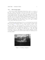
All the images used in this project are a cross-sectional view from the
skin (at the top) through the muscle to the bone (at the bottom), as can
be seen in figure 1.1. Tendons are seen as white structures, which look like
lines in a chestnut leaf. The intramuscular echo intensity reflects the amount
of muscle mass: when the structures around tendons are seen as black, it
means that there is a lot of muscle mass, which is a good sign. The ramus
is seen in the bottom of the image as a white line more or less wide. This
is the image of the bone. The ramus bone is seen quite distinctly on all the
copied images whether tendons and the muscle mass (echo intensity) is seen
in varying quality.
Figure 1.1: US image description
CHAPTER 1. INTRODUCTION
1.2
10
Materials and methods
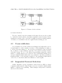
This project has been developed in cooperation with Dept. of Orthodonthy at the University of Geneva. The aim of this project was to define a
method to evaluate objectively the quality of the masseter muscle, which
was determined by Stavros Kiliaridis, PhD1 , in a four-point scale. Thus, the
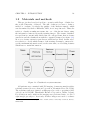
task is to classify an unknown texture into one of the known classes, using
the information extracted from the training images. The texture classification problem is conventionally divided into two sub-problems, that is, feature
extraction and the classification with the computed features (see figure 1.2).
Moreover, feature extraction part has an additional problem: feature selection, that is, to decide which features of the starting set must be extracted to
get the maximum information and, at the same time, avoid adding features
which have no useful information.
Figure 1.2: Classification system structure
All patients were examined with US imaging of masseter muscles with a
real-time scanner (Acuson, Acuson Corporation, Mountain View, CA, USA).
The real-time scans were printed on film paper by a videocopy printer (Mitsubischi, model PGGE, Mitsubischi Electric Corporation, Osaka, Japan).
For all subjects and conditions the imaging were performed twice, a total of
eight images per subject. Previously, all these images were used to evaluate
1
Professor and Chairman, Department of Orthodontics. University of Geneva, Genève,
Switzerland
CHAPTER 1. INTRODUCTION
11
the influence of the masseter muscle on the shape, thickness, bone mass and
trabeculation of the mandibular alveolar process. These images were scanned
to perform the analysis with a scanner (Epson,model Perfection 1200, Seiko
Epson Corporation, Seoul, Republic of Korea), with a resolution of 300*300
dpi. Image set was composed by 361 images, distributed as follows: 32 images of class 1, 81 of class 2, 136 of class 3 and 112 of class 4.
Image processing methods hold the potential to provide objective and
quantitative measures of US images. Previous studies by other groups have
identified texture analysis as being useful in the analysis of US images[1, 2, 3].
1.3
Organization
Chapter 2 presents how the muscle borders were found. A complete
explanation of the algorithm can be found, detailing information about subtechiques that have been used, such as fuzzy expressions. Qualitative results
are shown. Chapter 3 shows an introduction to texture analysis, as a feature extraction technique. A description of co-occurrence matrices and Laws
energy measures algorithms will be presented. Chapter 4 focuses on feature
selection and on classifier construction, and then results are presented and
discussed.
Chapter 2
Boundary Detection
Due to scattering and speckle noise, the shape of a border profile in a
US image can vary significantly. Finding maximal gradient points is an initial approach to the problem, but it does not work because it doesn’t takes
into account the connectivity of the boundary. Therefore, it is necessary to
find other mechanisms as well as ways of implementing them in a computerbased algorithm. Hence, the boundary detection system used in this project
was based in other systems already developed for more difficult cases, as the
boundary detection problem in US artery images [4, 5, 6]. Researchers in
this area propose a global approach to boundary detection. This global analysis is performed via the definition of a cost function containing information
about image features, which try to fit to human perception. Usually, human
perception works with really imprecise information. This imprecision can be
modeled with fuzzy expressions. Finally, human intervention can be useful
in two ways: as an a priori knowledge, it can be used to train the system;
as a posteriori knowledge, it can be used to solve ambiguous cases by direct
human assistance and including this information as a cost term in the cost
function.
2.1
Fuzzy Expressions
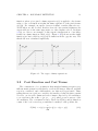
A fuzzy expression is a tool to mimic human global perception, which is
not linear. For example, human hearing doesn’t respond linearly to sound
activity; it does it logarithmically. So it is corrupting the input information.
That’s what fuzzy expressions do. Therefore, they transform a rigid criterion,
such as gradient or brightness, to a relaxed criterion that provides orientative
information. Thus, instead of using directly a feature value f (p) in the cost
12
CHAPTER 2. BOUNDARY DETECTION
13
function, where p is a pixel, a fuzzy expression µ(·) is applied to the feature
value, so the cost function weights the fuzzy expression of the pixel feature
µ(f (p)). For example, an expert observer wouldn’t consider faint echoes to
decide where are the borders. Besides, if an echo has certain brightness, the
expert will give it the same importance as other brighter echoes. In figure
2.1(a), we can see an example of this expert’s interpretation of an image
feature in a fuzzy function called µ1a (·). Figure 2.1(b) shows another fuzzy
function (we have called it µ2a (·)) those functions in the opposite way. The
thresholds were calculated empirically.
Figure 2.1: Two types of fuzzy expressions
2.2
Cost Function and Cost Terms
The construction of a cost function that matches human perception as a
full-automatic system is really hard to reach in US images. Instead, an MxN
region is considered, and a full analysis over this area is performed. Thus,
taking this area as a grid, we consider a deformable polyline BN that contains
N nodes, one in each column and each column composed by M candidates,
so we can denote BN as BN = {p1 , p2 , . . . , pN }, where pi can be anyone of the
M candidates. The cost function can be labeled as C(BN ), and is defined as
a sum of the local costs along a candidate boundary for the polyline BN
C(BN ) = cF (p1 ) +
N
X
i=2
(cF (pi ) + cG (pi−1 , pi ))
(2.1)
CHAPTER 2. BOUNDARY DETECTION
14
where local costs are composed by
cF (pi ) =
K
X
wi f˜j (pi )
(i = 1, . . . , N )
(2.2)
j=1
cG (pi−1 , pi ) = wk+1 gj (pi−1 , pi )
(i = 2, . . . , N )
(2.3)
in which f˜j (pi )(j = 1, . . . , K) are image feature terms, K is the number of
features used. The term cF refers to the cost associated with the computed
features and cG is related to geometric costs. We write f˜j (pi ) because they
are transformations of image feature values fj (pi ) with fuzzy expressions. If
we want every weight to be positive, we must define f˜j (pi ) so that a high
feature value at pi will result in a low f˜j (pi ) value, hence, a low local cost
that will attract the polyline. The term g(pi−1 , pi ) is called smoothness term,
because it takes in account vertical distance between two consecutive points
pi and pi−1 . Higher vertical distances will result in higher vertical values
and hence, a higher local cost will punish the connection between these two
points. It’s called smoothness term because it tries to keep the line smoother.
cN is the optimal BN that minimizes C(BN )
Hence, the resulting boundary B
bN = {BN | min(C(BN ))}
B
2.3
(2.4)
Dynamic Programming
Normally, the local-cost surface around the boundary that we are looking
for is not convex in a real image. This convexity appears severely distorted,
mainly in noisy images, such as US images. All the searching space must be
analyzed to avoid locking the solution in a local minimum. A straightforward
exhaustive search is necessary to succeed in finding the right solution, but it
is necessary to rewrite 2.1 to reduce the computational complexity from an
order of M N in terms of cost function evaluations. This can be solved by
defining 2.1 as a recursive expression:
C(p1 , 1) = cF (p1 )
(n = 1)
C(p1 , p2 , . . . , pn , n) = cF (p1 )
X
n−1
+
(cF (pi ) + cG (pi−1 , pi ))
i=2
+ {cF (pn ) + cG (pn−1 , pn )}
CHAPTER 2. BOUNDARY DETECTION
= C(p1 , p2 , . . . , pn−1 , n − 1)
+ (cF (pn ) + cG (pn−1 , pn ))
(n = 2, . . . , N )
15
(2.5)
Applying 2.5 instead of 2.1 the computational complexity is reduced to
an order of NxM 2 . To satisfy 2.4, we consider the candidate minima as a
cost function of the last node of BN (pn ):
C̃(pn , n) = minp1,...,pn {C(p1 , p2 , . . . , pn , n)}
(2.6)
If 2.5 is applied over 2.6, we can express it as a cost accumulation process
C̃(p1 , 1) = cF (p1 )
(n = 1)
C̃(p1 , p2 , . . . , pn , n) = minp1,...,pn−1 {C(p1 , p2 , . . . , pn−1 , n − 1)
+ (cF (pn ) + cG (pn−1 , pn ))}
= C̃(p1 , p2 , . . . , pn−1 , n − 1) + (cF (pn ) + cG (pn−1 , pn ))
(n = 2, . . . , N )
(2.7)
Accumulating costs according to 2.7, at each stage n, the location of pn−1
that defines C̃(pn , n), as expressed in 2.7, is recorded for each instance of pn .
bN defined in 2.4 can be found
Hence, the nodes of the optimal boundary B
by backtracking.
PbN = (pN | C(p1 , p2 , . . . , pN ) = minpN C̃(pN , N ))
Pbn−1 = (pn−1 | minn−1 {C̃(pn−1 , n − 1)
+ (cF (Pbn ) + cG (pn−1 , Pbn ))})
(n = N, . . . , 2)
(2.8)
(2.9)
where PbN refers to the selected point for pN (the last node) and Pbn−1 refers
to the selected points for the rest of the nodes.
2.4
Human Intervention
A human intervention mechanism becomes necessary when obvious errors
are detected. This method suggests adding human intervention as a member
of the cost function. This human intervention is introduced into the cost
function as an external force term defined as
cE (pk , qk ) = we d2 (pk , qk ).
(2.10)
CHAPTER 2. BOUNDARY DETECTION
16
It is a monotonously increasing function of the distance d between the
candidate node pk and the manually set point qk that has been inserted in the
kth column. Due to the smoothness, just one punctual setting has a global
effect over the whole trajectory of the boundary. The we weight decides the
attraction strength force. Thus, the initial definition of the cost function
(2.1) becomes
C(BN ) = cF (p1 ) +
N
X
{(cF (pi ) + cG (pi−1 , pi ))
i=2
Q
+
X
δ(i − kl )cE (pi , qkl )}
(2.11)
l=1
where Q is the number of user-set points (qk1 , qk2 , . . . , qkQ ) and δ(n) ensures that an extra term cE (·) is added only to the nodes that are in the
columns that have human-set points.
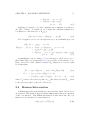
Figure 2.2: Human intervention effect in the cost function. Left figure shows
the cost function without any user points. A U-shaped gap appears centered
in where the point has been placed. Hence, the shape of the gap pushes the
boundary toward the point.
Figure 2.2 shows how this mechanism affects to cost function. The solid
line represents the detected border passing through the local cost surface.
This path is determined following the surface valley and, at the same time,
minimizing the curvature. Without any point set by the user (figure 2.2(a)),
the border has a different form than after setting one point (figure 2.2(b)).
A local U-shaped gap appears centered in the column where the point has
CHAPTER 2. BOUNDARY DETECTION
17
been set, forcing the border to modify its form from the original one. It is
important to notice that setting a point to modify the detected boundary
does not mean that the boundary will pass through this point. It just means
that the boundary will be pulled toward this point.
2.5
Implementation and Results
Three terms composed the cost function:
• Boundary smoothness: this term evaluated the number of rows that
separated two points pi−1 and pi :
g(pi−1 , pi ) = (pi−1y − piy )2
• Gradient value: lower values of gradient were punished. This term was
filtered with a fuzzy expression: µ1a (·), as defined in figure 2.1(a). This
gradient was computed with a 5 x 5 neighborhood and normalized. It
is also fitted to the intensity values within this window. The threshold
used in the fuzzy expression µ1a (·) was T1 = 0.4.
• User-set points: as told previously, this term punishes with the square
of the number of rows that a candidate point pi is far from a user-set
point in this same column i. A little modification has been added to for
a higher attraction: a users-set point affects to its column and to the
previous and following column, but in these cases with less intensity
(half intensity).
An improvement of the explained procedure has been applied in terms of
computing cost. Just a part of the image was analyzed when searching skin
and bone border, but additionally, for each analyzed point a little part of the
analyzed region was taken into account, reducing the cases to analyze, and
hence reducing the time expense.
No qualitative results have been computed, but figures 2.3, 2.4 and 2.5
are some examples of its functionality.
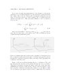
Figure 2.3 is a typical example of the human intervention effect over the
resulting skin border. Figure 2.3(a) shows the original image, and figure
shows the resulting border with only gradient and geometrical costs computed. This border has been bad calculated because other echoes, which
presented high gradient values, were enough close to become a candidate
CHAPTER 2. BOUNDARY DETECTION
18
border, and finally the system has selected it (figure 2.3(b)). Two points
were added by the user to attract the border (figure 2.3(c)): the left one to
avoid the three first echoes that appear almost aligned and are close to the
starting point. The second one to avoid the white cloud close to the ending
point that, because of its irregularity, it could be interpreted as the border.
Just with these two points the border fits correctly.
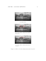
Figure 2.4 shows an example of a skin border that the system could find
correctly without human intervention. The original image (figure 2.4(a))
does not present strong echoes grouped, and it just appears a white cloud
quite regular near the starting point. In this case, the geometrical term is
enough to correct any possibility of selecting another possible candidate border (figure 2.4(b)).
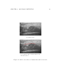
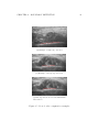
Normally, skin borders are more difficult to detect than the bone borders
because of tendinous structures (white clouds) that fall from the skin border.
The bone border is usually quite clear. In these cases no human intervention
is needed. An example is shown in figure 2.5(a). However, sometimes some
noise appears in the nearby of the bone border (figure 2.5(b)) and human
intervention is needed to avoid analyzing bone border points, if echoes are
below the bone border, or to maximize the analyzed area, if echoes are above
the bone border (figure 2.5(c)). Moreover, in section 4, muscle height and
width are used to decide muscle class, so it is important to correct this
possible mistakes.
CHAPTER 2. BOUNDARY DETECTION
(a) Original image
(b) Computed skin boundary without human
intervention
(c) Computed skin boundary with human intervention
Figure 2.3: Skin border where human intervention is needed
19
CHAPTER 2. BOUNDARY DETECTION
(a) Original image
(b) Computed skin boundary without human intervention
Figure 2.4: Skin border where no human intervention is needed
20
CHAPTER 2. BOUNDARY DETECTION
(a) Example of right edge detection
(b) Example of wrong edge detection
(c) Bad edge detection corrected with human
intervention
Figure 2.5: Bone border computation examples
21
Chapter 3
Textures
3.1
What is a Texture?
Many papers on texture analysis begin with stating that there exists no
precise definition of Texture. Others don’t give any definition or give a definition that suits to the method that they present. The intuitive nature of
the term can be a reason and, moreover, it becomes really hard to capture
these imprecisions in a concrete definition. Anyway, some definitions have
been presented in image processing handbooks and texture papers. Some
examples can be found in [7, 8, 9, 10, 11, 12].
Even with this difficulty to get a definition, texture is a term widely
used and well understood in common language. The term is usually used
to describe intrinsic properties of an object, such as granulation, roughness,
coarseness, etc. So it could be defined as something consisting in mutually
related elements, or more formally, a set of local neighborhood properties.
Hence, it can be stated that when we talk about textures we are considering
a group of pixels, sometimes called texture primitive or texture element, and
the texture described is highly dependent on the number of pixels considered
(the texture scale)[13]; texture description is scale dependent.
3.2
3.2.1
Texture Analysis
Introduction
The main aim of texture analysis is texture recognition and texture-based
shape analysis. Such features can be found in the tone (brightness in gray22
CHAPTER 3. TEXTURES
23
level images) and in the structure of a texture[13]. Tone is mostly a single
pixel feature. Besides, structure is the relationship between them but, however, tone and structure are not independent. Figure 3.1 shows an example:
figures 3.1(a) and 3.1(b) have the same number and type of elements, but
they don’t have the same texture; besides, figures 3.1(a) and 3.1(c) have the
same spatial relationship of elements, but again they show different textures.
Figure 3.1: Textures with tonal or structural similarities
3.2.2
Utility
Texture analysis plays an important roll in areas such as scene analysis,
medical image analysis, remote sensing and other application areas. Texture
analysis is used in the following tasks:
• the classification of images based on their textural appearance (this
project is an example of this tasks);
• the segmentation of images into regions, which have similar textural
properties;
• other information extraction from textural cues, e.g. for reconstructing
3D scenes from 2D scenes.
Image classification is the basic task that deals with associating images as
a whole with classes from a predefined set. Image segmentation is a localized
version of image classification, because every pixel of an image is classified
individually or in small groups.
3.2.3
Texture Analysis Techniques
Several texture analysis techniques exist, but two main texture description approaches can be identified: statistical and syntactic[13].
CHAPTER 3. TEXTURES
24
Statistical methods gather information about textures exploiting pixels
statistics: this can be first order statistics, such as mean and variance, but
more importantly higher order statistics, mostly second order. These methods compute different properties, such as directionality or periodicity, and
are suitable if texture elements sizes are comparable with the pixel sizes.
Syntactic and hybrid methods (combination of statistical and syntactical
methods) are more suitable where texture elements can be assigned a label
(their type). In these cases, texture elements can be described not only using
tonal properties, but also using a larger variety of them.
From now on, syntactical methods are let aside in favor of statistical
methods, which have been used in our system. This selection has been done
because texture elements are comparable with the pixel size, so statistical
methods fit better than the syntactical methods. Additionally, previous research projects have shown statistical texture analysis to fit well to US images
[14, 15, 16].
3.2.4
Statistical Methods
Several statistical texture analysis methods have been described, such as:
• autocorrelation texture description, which is based on spatial frequencies, describing their organization by a correlation coefficient that evaluates linear spatial relationships between texture elements. A single
pixel is considered as a texture element and its tone property is the
gray-level;
• co-occurrence matrices method of texture description is based on the
repeated occurrence of some gray-level configuration in the texture (see
section 3.3);
• edge frequency method is obviously based in edge detection with any
edge detector for different distances (texture is scale dependent, 3.1);
• primitive run length method is based in catching a large number of
constant-gray-levels pixels in a located line;
• Laws’ texture energy measures method is based in determining texture
properties by assessing average gray-level, edges, spots, ripples and
waves in texture(see section 3.4);
CHAPTER 3. TEXTURES
25
• fractal texture description is based in correlation between texture coarseness and fractal dimension of a texture, as demonstrated in [17].
3.3
Co-occurrence Matrices
The co-occurrence matrices method of texture description, also called
Haralick’s method and spatial gray-level dependency matrices, is a secondorder statistical approach. It is based on the repeated occurrence of some
gray-level configuration in the texture. Textural features are derived from
angular nearest-neighbor spatial-dependence matrices[18]. This method has
become one of the most well known and it is widely used for texture description.
A co-occurrence matrix is the joint probability of occurrence of gray levels
i and j for two pixels with a defined spatial relationship in an image. This
spatial relationship is defined in terms of distance d and orientation φ.
Let D be the part of an image to be analyzed which size is MxN. An
occurrence of some gray-level configuration can be described as a matrix of
relative frequencies Pφ,d (a, b), representing the number of times two pixels
with gray-levels a and b occur in D separated by a distance d and orientation
θ, from each other. These matrices are not symmetric, but usually are defined
as Pφ,d (a, b) = Pφ,d (a, b)+Pφ,−d (a, b), resulting a formulation as shown below,
to avoid this asymmetry and reducing the number of matrices to compute
from 8 to 4. Hence, non-normalized definitions of co-occurrence as functions
of angle and distance can be represented formally as
P0o ,d (a, b) = | {{(k, l), (m, n)} ∈ D :
k − m = 0, | l − n |= d, f (k, l) = a, f (m, n) = b} |
P45o ,d (a, b) = | {{(k, l), (m, n)} ∈ D :
(k − m = d, l − n = −d)OR(k − m = −d, l − n = d),
f (k, l) = a, f (m, n) = b} |
P90o ,d (a, b) = | {{(k, l), (m, n)} ∈ D :
| k − m |= d, l − n = 0, f (k, l) = a, f (m, n) = b |
P135o ,d (a, b) = | {{(k, l), (m, n)} ∈ D :
(k − m = d, l − n = d)OR(k − m = −d, l − n = −d),
(3.1)
f (k, l) = a, f (m, n) = b} |
CHAPTER 3. TEXTURES
26
where | {. . .} | refers to set cardinality.
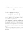
As an example, let’s consider the following 4x4 image containing 3 different gray values:
1
1
0
0
1
1
0
0
0
0
2
2
0
0
2
2
The 3x3 gray-level co-occurrence matrices for this image for orientations
θ = 90o and θ = 135o and distance d = 1 are given below:
8 2 2
4 2 2
P90o ,1 = 2 4 0
P135o ,1 = 2 2 1
2 0 4
2 1 2
The element P90o ,1 (0, 2) represents the number of times two pixels with
gray-levels 0 and 2 and separated by distance 1 appear in direction 90o :
P90o ,1 (0, 2) = 2. Similarly, P135o ,1 (2, 1) counts the number of appearances of
two pixels with gray-levels 2 and 1, separated by distance 1; so P135o ,1 (2, 1) =
1. The rest of matrices are built in the same way.
If the texture is coarse and distance d is small compared to the size of
the texture elements, the pairs of points at distance d should have similar
gray levels. Inversely, for a fine texture, if distance d is comparable to the
texture size, then the gray levels of points separated by distance d should
often be quite different, so that values in the co-occurrence matrix should be
spread out relatively uniformly. Therefore, a good way to analyze texture
coarseness would be, for various values of distance d, some measure of scatter
of the matrix around the main diagonal. Similarly, if the texture has some
direction (coarser in one direction than another) then the degree of spread
of the values about the main diagonal in the matrix should vary with the
direction d.
Haralick proposed some texture features to be extracted from co-occurrence
matrices. Different authors have used them with different names, so it is
better just keep in mind that these features take information to form a classification criteria.
CHAPTER 3. TEXTURES
3.4
27
Laws’ Texture Energy Measures
Certain gradient operators such as Laplacian and Sobel operators remark
the underlying microstructure of texture within an image. This method is
based in a similar principle. It uses series of pixel impulse response arrays
obtained from combinations of one-dimensional vectors[19]. These vectors
are derived from three base vectors
L3 = (1, 2, 1)
E3 = (−1, 0, 1)
S3 = (−1, 2, −1)
(3.2)
which represents, respectively, averaging (level), first difference (edges) and
second difference (spots). If it is necessary to obtain longer vectors to analyze
an image in different scales, a convolution of these vectors with themselves
and each other must be applied until we obtain the desired length. After
first convolution, five vectors result
L5
E5
S5
R5
W5
=
=
=
=
=
(1, 4, 6, 4, 1)
(−1, −2, 0, 2, 1)
(−1, 0, 2, 0, −1)
(1, −4, 6, −4, 1)
(−1, 2, 0, −2, 1)
(3.3)
which are associated to and underlying microstructure and labeled with
acronyms accordingly (L to Level, E to Edge, S to Spot, W to Wave and
R to Ripple).
The two-dimensional convolutional kernels (named 5x5 Laws’ masks) resulted from multiplying these length-five vectors, by transposing the first
vector term and leaving the second term as a row vector. They are applied
to the digital image to get the measures, and then a nonlinear windowing
operation is performed. After this convolution, we obtain 25 different twodimensional convolutional kernels. As an example the L5E5 kernel is found
by convolving L5 vector with the E5 vector. A listing of all 5x5 kernel names
is given below:
L5L5
L5E5
L5S5
L5W5
L5R5
E5L5
E5E5
E5S5
E5W5
E5R5
S5L5 W5L5 R5L5
S5E5 W5E5 R5E5
S5S5 W5S5 R5S5
S5W5 W5W5 R5W5
S5R5 W5R5 R5R5
CHAPTER 3. TEXTURES
28
The next step is dedicated to explain how to compute the texture energy
measures over a digital image.
3.4.1
Laws Algorithm
Let D be a NxM digital image that we want to analyze with regards to
its texture properties. We first apply each of the 25 convolutional kernels to
the image, resulting in a set of 25 NxM gray-level images, which will be the
basis for the textural analysis. Next, we replace every pixel in the 25 NxM
separate grayscale images with Texture Energy Measure (TEM) at the pixel.
We do that by applying a nonlinear windowing to the set of 25 NxM images,
resulting a new set of 25 NxM images, which we will refer to as TEM images.
Laws suggest two nonlinear filters:
5
5
X
X
| BaseImage(x + i, y + j) |
(3.4)
v
u 5
5
uX X
t
TEM(x, y) =
BaseImage2 (x + i, y + j)
(3.5)
TEM(x, y) =
i=−5 j=−5
i=−5 j=−5
At this point, again, we have 25 new images (TEM images) that we will
name with the original convolution kernels with an appended ”T”, to indicate
that they are texture energy measures and to make any reference to them
easier. Thus, the TEM images are named as follows:
L5L5T
L5E5T
L5S5T
L5W5T
L5R5T
E5L5T
E5E5T
E5S5T
E5W5T
E5R5T
S5L5T
S5E5T
S5S5T
S5W5T
S5R5T
W5L5T
W5E5T
W5S5T
W5W5T
W5R5T
R5L5T
R5E5T
R5S5T
R5W5T
R5R5T
In some applications, texture directionality is not important. In this
case, similar features can be combined to remove directional information.
For example, while L5E5 is sensitive to vertical edges, E5L5 is sensitive to
horizontal edges. Adding these TEM images, we have a new single feature
sensitive to ”edge content” in a general sense. If we want to work with these
”general-sense” features, TEM images generated with transposed convolution
kernels are added together. Lets denote these new images with an appended
”R” meaning ”rotational invariance”. We will call this images TR images.
CHAPTER 3. TEXTURES
E5L5TR
S5L5TR
W5L5TR
R5L5TR
S5E5TR
W5E5TR
R5E5TR
W5S5TR
R5S5TR
R5W5TR
=
=
=
=
=
=
=
=
=
=
E5L5T
S5L5T
W5L5T
R5L5T
S5E5T
W5E5T
R5E5T
W5S5T
R5S5T
R5W5T
29
+ L5E5T
+ L5S5T
+ L5W5T
+ L5R5T
+ E5S5T
+ E5W5T
+ E5R5T
+ S5W5T
+ S5R5T
+ W5R5T
There are five remaining cases, which are scaled by 2 to keep all features
consistent.
E5E5TR
S5S5TR
W5W5TR
R5R5TR
L5L5TR
=
=
=
=
=
E5E5T
S5S5T
W5W5T
R5R5T
L5L5T
*
*
*
*
*
2
2
2
2
2
L5L5T is usually discarded when no contrast information is needed, and
this information is used to scale the other TEM images pixel by pixel. At
this point we have a set of 15 texture features (14, when L5L5T is discarded),
which are rotational invariant. Another possibility is keeping directional information and work with a set of 25 TEM images, which will be the texture
feature set. Whatever the process followed, at this point, we get a data set
where every pixel is represented by M texture features, where M can be
14, 15 or 25, depending on which process was applied. Another step can be
applied to get more information. It is possible to apply a statistical analysis
over the remaining images (texture features) to get information about the
distribution of these images. Thus, if we have M remaining images and we
get N statistical values from each one, we finally get MxN statistical texture
features from the original images.
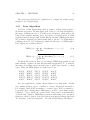
3.5
Implementation and Results
In this chapter, both algorithm implementations are commented and extracted features are presented. Additionally, some images samples are pre-
CHAPTER 3. TEXTURES
30
sented of resulting co-occurrence matrices and Laws TR images.
Co-occurrence matrices
Several features were computed in both co-occurrence matrices and Laws
methods.
For the co-occurrence matrix method, matrices were computed for distances 3, 5 and 7 and directions 0o , 45o , 90o , 135o and the all of them added,
to find some rotational-invariant features. For each matrix, the following 11
features were computed1 :
Energy =
XX
i
XX
Contrast =
XX
i
(3.6)
Pφ,d (i, j)log2 (Pφ,d (i, j))
(3.7)
(i − j)2 Pφ,d (i, j)
(3.8)
j
Entropy =
i
P2φ,d (i, j)
j
j
X X Pφ,d (i, j)
IDM =
1 + (i − j)2
i
j
X X
M ean(µ) =
i
Pφ,d (i, j)
i
Standarddeviation(σ) =
X
(i − µ)2
ClusterShade =
Pφ,d (i, j)
j
σ2
(3.12)
((i − µ) + (j − µ))3 Pφ,d (i, j)
(3.13)
((i − µ) + (j − µ))4 Pφ,d (i, j)
(3.14)
j
XX
i
(3.11)
j
XX
i
ClusterP rominence =
X
X X (i − µ)(j − µ)Pφ,d (i, j)
i
(3.10)
j
i
correlation(ρ) =
(3.9)
j
X X (| i − j | ((i − µ) + (j − µ))Pφ,d (i, j)
DiagonalM oment =
2(1 + ρ)σ 2
i
j
(3.15)
1
both µ and σ correspond to µx and σx each, but they have the same value as µy and
σy when working with symmetric matrices, so lets call them just µ and σ. Thus, every
equation that contained this values have been redefined accordingly
CHAPTER 3. TEXTURES
SumCorrelation =
31
X X (i − µ)(j − µ)((i − µ) + (j − µ))Pφ,d (i, j)
p
σ 3 2(1 + ρ)
i
j
(3.16)
Some of these features are quite well known, such as energy, entropy,
mean, standard deviation or correlation. For the others, an explanation is
presented:
• Contrast is a measure of local image variations.
• IDM (Inverse Different Moment) is a measure of the uniformity of
an image: homogeneous images are represented with high values, and
heterogeneous ones are represented by low values.
• Cluster Shade is a 2-D version of the gray-level histogram skewness.
Skewness measures the degree of asymmetry of a distribution.
• Cluster Prominence is a 2-D version of the gray-level histogram kurtosis. Kurtosis measures how peaked is a distribution.
• Diagonal Moment measures the differences in correlation for high and
low gray levels.
• Sum Correlation measures the asymmetry of the distribution along the
diagonal of the co-occurrence matrix.
Thus, 165 features (3 different distances * 5 directions * 11 features for
each case) were extracted from the co-occurrence matrix method.
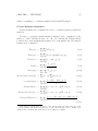
It’s quite interesting to see how co-occurrence matrices vary with distances and with directions for one image and to compare how they differ
from one class to another. The following figures (3.2) are samples of a class
4 image: figure 3.2(a) shows matrices for θ = 0o for the three analyzed distances; figure 3.2(b) for θ = 45o ; figure 3.2(c) for θ = 90o ; figure 3.2(d) for
θ = 135o ; figure 3.2(e) for all the unrotational one.
In a good quality muscle, tendinous structures (white stripes) must be
clear and must be surrounded by black structures (muscle). This can be seen
in these co-occurrence matrices: for all the analyzed directions, two small
clouds of points over the diagonal can be clearly discerned. The first one,
starting from the top left of the image, is associated to the black structures
that surround the white stripes. The second one corresponds to the white
stripes and the transition from white to black structures. It is also clear that
CHAPTER 3. TEXTURES
32
(a) θ = 0o
(b) θ = 45o
(c) θ = 90o
(d) θ = 135o
(e) Unrotational case
Figure 3.2: Co-occurrence matrices samples for quality 4
CHAPTER 3. TEXTURES
33
this transition is done quite fast because few intermediate gray level appear.
It can be also noticed how the matrices are more dispersed when incrementing distance. This is how this matrices show that distance is getting close to
elements size.
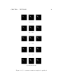
Figure 3.3 presents a similar analysis, but in this case an interclass analysis is presented. In this example just one direction is analyzed (θ = 45o ),
but it can be applied to all of them. In all the cases, more disperse matrices appear when incrementing distance. This effect is less clear in lower
qualities. This can be explained because element sizes are smaller than in
higher qualities. In quality 3 example, the transition between white black
structures is slower, but higher gray levels are present. In quality 2 example,
a small concentration can be seen as black structures and transition to these
structures is done quite fast, but higher gray levels are quite dispersed. This
could mean that original image has several echoes with medium brightness
and not clear stripes. In quality 1 example, only medium gray levels are
presented, so no clear structures can be seen.
CHAPTER 3. TEXTURES
34
(a) Quality 4
(b) Quality 3
(c) Quality 2
(d) Quality 1
Figure 3.3: Co-occurrence matrices comparation for all qualities
CHAPTER 3. TEXTURES
35
Laws energy measures
The five features extracted from each resulting image were:
XX
Energy =
TRimage(i, j)
i
(3.17)
j
1 XX
M ean(µ) =
TRimage(i, j)
MN i j
XX
1
V ariance =
(TRimage(i, j) − µ)2
(M − 1)N i j
(3.18)
(3.19)
Skewness =
1 X X (TRimage(i, j) − µ)3
3
MN i j
V ar 2
(3.20)
Kurtosis =
1 X X (TRimage(i, j) − µ)4
MN i j
V ar2
(3.21)
It is important to note that we have named Energy a feature that adds
directly the values instead of their squares. We have done it in this way
because this feature adds energy measures. Skewness and kurtosis are briefly
explained in the description of diagonal moment and sum correlation features
of co-occurrence matrices algorithm.
As a first approximation to the problem, we started working with the
rotational invariant set of kernels to avoid managing too many features at
the same time (165 co-occurrence features + 15 TR images * 5 features from
each case, throws an amount of 240 features, a number comparable to the
number of samples). The rotational variant case was also checked, but it
gave worse results than the rotational invariant case (in this case, a total of
125 features were computed, 25 images * 5 features from each image).
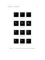
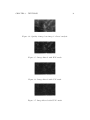
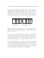
Figures 3.5 to 3.19 show an example of the effect of each kernel over
the quality 4 image presented in figure 3.4. No other class examples are
presented because it is hardly difficult to get significant visual information,
so no comparations can between classes has been done.
CHAPTER 3. TEXTURES
Figure 3.4: Quality 4 image base image for Laws’ analysis
Figure 3.5: Image filtered with E5L5 mask
Figure 3.6: Image filtered with S5L5 mask
Figure 3.7: Image filtered with W5L5 mask
36
CHAPTER 3. TEXTURES
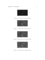
Figure 3.8: Image filtered with R5L5 mask
Figure 3.9: Image filtered with S5E5 mask
Figure 3.10: Image filtered with W5E5 mask
Figure 3.11: Image filtered with R5E5 mask
37
CHAPTER 3. TEXTURES
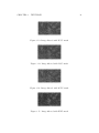
Figure 3.12: Image filtered with W5S5 mask
Figure 3.13: Image filtered with R5S5 mask
Figure 3.14: Image filtered with R5W5 mask
Figure 3.15: Image filtered with E5E5 mask
38
CHAPTER 3. TEXTURES
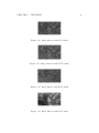
Figure 3.16: Image filtered with S5S5 mask
Figure 3.17: Image filtered with W5W5 mask
Figure 3.18: Image filtered with R5R5 mask
Figure 3.19: Image filtered with L5L5 mask
39
Chapter 4
Feature Selection and Classifier
Construction
Feature selection is one of the main problems in signal processing, because extracting features (characteristics) isn’t enough. This term, feature
selection, refers to the selection of an optimum subset of features, and hence
it is related to input dimensionality and parameter reduction problems.
Feature selection is motivated, at least, for these three main reasons:
• Many of the features are hardly correlated. Others are directly related,
such as voltage and current in an electrical system.
• Some features may simply be unrelated to the problem, and hence
adding noise to the system.
• Reduce computational costs, specially in real-time applications.
A good definition of feature selection is given in [20]: Feature Selection
is a process that attempts to select a subset of features, satisfying a combination of application and methodology-dependent criteria: minimizing the
cardinality of the feature subset; ensuring classification accuracy does not significantly decrease; and approximating the original class distribution with the
class distribution given the selected features.
A feature selection scheme can be summarized as follows: feature subsets
are somehow generated and evaluated until a stopping criterion is satisfied
(figure 4.1).
There exists lots of ways of generating feature subsets. Any of them can
be applied to decide candidate subsets: from exhaustive to evolutionary and
40
CHAPTER 4. FEATURE SELECTION AND CLASSIFIER CONSTRUCTION41
Figure 4.1: Feature selection scheme
stochastical methods.
We use a method were the training and feature selection work together
to obtain the desired subset, involving sequential forward selection and a
classification criteria. Due to the lack of samples in relation with the number
of features, cross-validation was also applied in the training process.
4.1
Cross-validation
Cross-validation is a really well known technique used when there are not
enough samples to train a system correctly, so that resampling is a must, or
to check a net performance[21]. In a k-fold cross-validation, data is divided
into k subsets of, approximately, equal size. The system is trained k times,
each time leaving out one of the subsets from training, using this omitted
subset to compute whatever error criterion. The k individual estimations are
averaged, using this final result as the error estimation. Another possibility is
training weights, so the averaging is applied to the resulting weights instead
of the error, so the final result is an estimation of the weights.
4.2
Sequential Forward Selection
Unlike exhaustive search, sequential forward selection (SFS) is always
computationally tractable. Even in the worst case, it checks a much smaller
number of subsets before finishing. This technique adds predictor variables
and never deletes them.
CHAPTER 4. FEATURE SELECTION AND CLASSIFIER CONSTRUCTION42
First, forward selection uses an empty set as starting subset. At the first
step, FS evaluates N variable subsets, each consisting of a single variable,
and selecting the one with the highest evaluation criterion. In this case, the
evaluation criterion is the classification, so the variable that classifies better
the images is selected. At the next step, it makes a selection among N-1
subsets, the next step from N-2 subsets, and so on. If all predictor variables
are selected, at most N(N+1)/2 subsets are evaluated before the search ends.
The problem with SFS is that, unlike exhaustive search, it is not guaranteed
to find the subset with the highest evaluation criterion. In practice, however,
many researchers have reported good results with forward selection
4.3
Classifier Construction and Results
Both training and validation steps were calculated in a MATLAB environment and further checked with the final application.
A combination of SFS with cross-validation was used in the training process. At each step of the SFS and for each analyzed case, mean square
error minimization was applied to compute the system weights at each crossvalidation step. Thus, let yobj be a vector containing the expected values for
each image of the validation set. Let y be the resulting values for each image
of the validation set. Hence, the function C to minimize is:
C = k yobj − y k2
(4.1)
Texture analysis was performed over a rectangle located between skin
and bone borders. This rectangle has as top limit the lower vertical value
of the skin border, and as bottom limit the higher vertical value of the bone
border. Similarly, left limit has the higher horizontal value of both skin and
bone border, and right limit the lower horizontal value of both borders. To
avoid analyzing border points, a security margin of 5 pixels is used both in
height and width.
Each class was mapped to a number: 1 for class 1, 2 for class 2, and
so on. Thus, all the available data were labeled with their class. Both in
training and validation steps, these labels were used as goal functions. The
selected criteria to decide the image class was the distance to the labels, so
the resulting value of applying the resulting weights to their related features
of an image was expected to be close to its label. The selected labels were 1,
2, 3 and 4, so the threshold levels were 1.5 (limit between class 1 and 2), 2.5
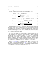
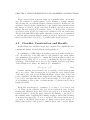
(limit between class 2 and 3) and 3.5 (limit between class 3 and 4). Figure
CHAPTER 4. FEATURE SELECTION AND CLASSIFIER CONSTRUCTION43
4.2 shows validation results at each step. The best results were achieved
for 28 features, with an 85.71% when success in classificating images of the
validation set. It shows also that after this maximum, the system becomes
over-trained and worse results are obtained.
Figure 4.2: Classification results of the selected classifier. With 28 features
the maximum classification rate is reached (85.71%)
Selected features were:
• Co-occurrence matrices (18):
– d = 3, φ = 0: correlation and sum correlation
– d = 5, φ = 0: contrast and diagonal moment
– d = 7, φ = 0: energy and diagonal moment
– d = 3, φ = 45: energy
– d = 5, φ = 45: diagonal moment
– d = 7, φ = 45: energy, entropy, IDM and diagonal moment
– d = 5, φ = 90: contrast
– d = 7, φ = 90: IDM, correlation and diagonal moment
– d = 5, φ = 135: contrast
CHAPTER 4. FEATURE SELECTION AND CLASSIFIER CONSTRUCTION44
– d = 7, φ = 135: correlation
• Laws’ energy measures(7):
– S5L5: energy
– W5E5: variance
– R5S5: kurtosis
– S5S5: variance
– W5W5: variance and skewness
– R5R5: skewness
Additionally, size features were included in the analysis and also selected:
area, height and width.
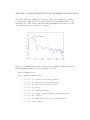
It must be noticed that more than half of the features from the cooccurrence matrices (10 out of 18) correspond to distance 7, so a new analysis
was performed including matrices for distances 9 and 11. Results are shown
in fig 4.3. An 85.71% was again the result, including just one feature for
distance=11, but with 23 features instead of 28.
Figure 4.3: Classification results of the other classifier. With 23 features the
maximum classification rate is reached (85.71%)
CHAPTER 4. FEATURE SELECTION AND CLASSIFIER CONSTRUCTION45
This reduction in the number of selected features could lead to decide to
implement this new classifier instead of the selected one, but additional requirements had to be fitted, such as minimizing error impact between classes.
This means that when failing in deciding an image class, this error should
not be higher than one class. For example, an image of class 2 should not
be classified as a class 4, but class 1 or 3 could be acceptable. Hence, an
additional test was performed to check it. Results are presented in figure 4.4.
Class
1
2
3
4
1 2 3 4
2 5 1 0
0 20 1 0
0 3 30 1
0 0 2 26
(a) Results of the implemented classifier
Class
1
2
3
4
1 2 3 4
4 4 0 0
0 21 0 0
2 3 28 1
0 0 3 25
(b) Results when computing co-occurrence matrices
for d = 9, 11
Figure 4.4: Classification results class by class for implemented classifier
(figure 4.4(a)) and for classifier computing co-occurrence matrices for d =
9, 11, (figure 4.4(b)). Row indexes identify real classes. Column indexes
identify selected classes
It can be seen that in both cases, images of class 1 are worse classified
than images of the other classes. This is not surprising, because there were
less images of this class than the others, as it has been explained in section
1.2 (Materials and Methods). The differences between both analyzed cases
are not really significant, but one more critical error (errors of more than one
class) appear when computing co-occurrence matrices for d = 9, 11.
As a final remark, it must be noticed that it was added in the final application the possibility of classifying an image in two classes. This possibility
is activated when an image is near a threshold. In these cases, two classes
appear as result: the first class (primary class) is the one normally selected;
the second one (secondary class) is the class at the other side of the threshold. For example, if the resulting value of a classification is 2.6, close to 2.5
threshold, the primary class is 3 and the secondary class is 2.
Chapter 5
Conclusions
5.1
Achievements
In this work we have presented the implementation of a classifier for
US images of the masseteric muscle. This classifier has been implemented
following this steps:
1. locate the muscle via detecting its borders
2. application of a texture analysis over a selected region of the muscle
3. combine linearly the extracted features and mapping the result to a
class (or classes)
4. developement of an interface for automatic classification
Feature selection was developed by combining sequential forward selection
with cross-validation, in order to find which features contained classification
information and to decide their importance, by computing their associated
weights.
Dual class results are presented when system computes ambiguous results.
This additional functionality permits receiving more accurate information in
classification terms. Finally, it was also achieved to compute few critical results.
5.2
Future Work
Due to the nature of the application, it can be easily adapted to other
US muscle images. It just needs a set of previously classified images. In
46
CHAPTER 5. CONCLUSIONS
47
this point, it must be noticed that in training step, muscle selected area was
decided by a non-expert user, so this must be taken into account for any
future developement, because it can be useful to get a better trained system
and, hence, to get a better classifier.
Another possible improvement could be developing full automatic classifier, automatically detecting muscle borders.
It is also possible to insert the application in the US machine. If this
improvement were combined with the automatical border detection, it could
be possible to have an US machine with a healthy integrated classifier. This
improvement is closely related with another problem that could not be solved
because of the nature of the provided images. In an integrated application,
there is no need of printing the image and then scan it. These steps also
adds noise to the original sample and better results could be reached if they
were eliminated.
Appendix A
User Manual
When executing the program, a browser appears to select the desired image. It must be a scanned image, at 300x300dpi of resolution and then it
must be saved in .bmp format, with 24 bits per pixel. Any comercial scanner
can fit these requirements.
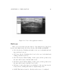
Once the image has been selected, a window appears containing the central part of the selected image. Figure A.1 is shown as example.
Menu options
There are two options in the menu bar: Muscle capture and Image Mode
(figure A.2).
• Muscle capture offers the possibility of selecting the image area where
the analysis will be performed by selecting the borders (Borders option)
or directly by selecting four points to directly configure the rectangle
(Rectangle option).
• Image mode offers the possibility to analyze images directly extracted
from an US machine or scanned images previously printed. This menu
is disabled. It has been included for further improvements.
Menu options must be selected before usign any other part of the application.
48
APPENDIX A. USER MANUAL
49
Figure A.1: View of the application window
Buttons
There are seven buttons in the window: Calc Skin Border, Calc Bone
Border, Mod Skin Border, Mod Bone Border, OK, AREA and RESET.
• Calc Skin Border Calculates the skin border once both initial and ending point have been set.
• Calc Bone Border Calculates the bone border once both initial and
ending point have been set.
• Mod Skin Border When clicking on this option, all the points set by
the user will be used to find the skin border.
• Mod Bone Border When clicking on this option, all the points set by
the user will be used to find the bone border.
• OK Once both borders have been calculated or the area has been directly selected, clicking this button computes image class.
• AREA This button is used to directly set the area to be analyzed.
APPENDIX A. USER MANUAL
50
Figure A.2: Menu contents of the application
• RESET By clicking this button a browser is opened to select a new
image (or the same) to analyze.
It must be noticed that options selected in the menu affect those buttons.
If Rectangle option has been selected, Calc Skin Border, Calc Bone border,
Mod Skin Border and Mod Bone border buttons do not work. If Borders
options is selected, AREA button do not work.
General Procedure
There are two possible procedures depending on which Muscle capture
option is selected:
1. Computing borders: there is no problem with starting calculating skin
or bone border. To compute the skin border, first click on Mod Skin
Border button. Then starting and ending points must be set. At this
point, skin border can be calculated by clicking on Calc Skin Border
button. If the resulting border does not fit to the real one, additional
points can be set to help the program to get it. These point shoul be
APPENDIX A. USER MANUAL
51
set in areas to which program cannot compute, such as whithe thick
stripes close to the border. These points can be set before calculating
any border. Points are set by left clicking on the image. Right clicking
will remove the closest user-set point. The same process must be done
to compute tha bone border but using Mod Bone Border and Calc Bone
Border buttons. Once both borders have been selected clicking on OK
button will perform the classification of the muscle.
2. Area selection: select four points to define the rectangular area to be
analyzed. The highest restricting conditions will be applied (minimum
upper value, maximum lower value, etc.). Once these points are set,
clicking on OK button will perform the classification of the muscle.
For any doubts, please contact: [email protected]
Bibliography
[1] N.-D. Kim, V. Amin, D. Wilson, G. Rouge, and S. Udpa, “Multiresolutional texture analysis for ultrasound tissue characterization,” Nondestructive Testing and Evaluation, special issue on Biomedical applications, no. 4, pp. 201–215, 1998.
[2] N.-D. Kim, L. Booth, V. Amin, J. Lim, and S. Udpa, “Ultrasonic image
processing for tendon injury evaluation,” Proceedings of the IEEE-SP
International Symposium on Time-Frequency and Time-Scale analysis,
USA, 1998.
[3] M. Masseroli, M. Cothren, D. Meier, and et al., “Quantification of intramural calcification in coronary intravascular ultrasound images with
automated image analysis,” Am Heart J, vol. 136, no. 1, pp. 78–86, 1998.
[4] T. Gustavsson, Q. Liang, I. Wendelhag, and J. Wikstrand, “A dynamic
programming procedure for automated ultrasonic measurement of the
carotid artery,” Proceedings IEEE Computers Cardiology, pp. 297–300,
1994.
[5] R. J. Kozick, “Detecting interfaces on ultrasound images of the carotid
artery by dynamic programming,” SPIE, pp. 233–241, 1996.
[6] Q. Liang, I. Wendelhag, J. Wikstrand, and T. Gustavsson, “A multiscale
dynamic programming procedure for boundary detection in ultrasonic
artery images,” IEEE Transactions on Medical Imaging, no. 2, pp. 127–
142, 2000.
[7] J. Slansky, “Image segmentation and feature selection,” IEEE Transactions on Systems, Man and Cybernetics, no. 4, pp. 237–247, 1978.
[8] B. Jahne, “Digital image processing.”
[9] Wilson and Spaan, “Image segmentation and uncertainty.”
[10] A. K. Jain, “Fundamentals of image processing.”
52
BIBLIOGRAPHY
53
[11] R. C. Gonzalez and R. E. Woods, “Digital image processing.”
[12] I. S. 610.4-1990, “Ieee standard glossary of image processing and pattern
recognition terminology,” IEEE Press, New York, 1990.
[13] R. M. Haralick, “Statistical and structural approaches to texture,” Proceedings IEEE, vol. 67, no. 5, pp. 786–804, 1979.
[14] U. Raeth, D. Schlaps, B. Limberg, I. Zuna, A. Lorenz, G. van Kaick,
W. J. Lorenz, and B. Kommerell, “Diagnostic accuracy of computerized b-scan texture analysis and conventional ultrasonography in diffuse
parenchymal and malignant liver disease,” J. Clin. Ultrasound, pp. 87–
99, 1985.
[15] F. M. J. Valckx and J. M. Thijssen, “Texture classification of echographic images by means of the co-occurrence matrix,” Acoust. Imag.,
pp. 299–302, 1996.
[16] C.-M. Wu, Y.-C. Chen, and K.-S. Hsieh, “Texture features for classification of ultrasonic liver images,” IEEE Transactions on Medical Imaging, pp. 141–152, Apr. 1992.
[17] A. P. Pentland, “Fractal-based description of natural scenes,” IEEE
Transactions on Pattern Analysis and Machine Intelligence, no. 6,
pp. 661–674, 1984.
[18] R. M. Haralick, K. Shanmugam, and I. Distein, “Textural features for
image classification,” IEEE Transactions on Systems, Man and Cybernetics, no. SMC-3, pp. 610–621, 1973.
[19] K. Laws, “Textured image segmentation,” Ph.D. Dissertation, University of Southern California, January, 1980.
[20] M. Dash and H. Liu, “Feature selection for classification,” Intelligent
Data Analysis - An International Journal, no. 3, pp. 374–385, 1997.
[21] G. Torheim, F. Godtliebsen, D. Axelson, K. A. Kvistad, A. Haraldseth, and P. A. Rinck, “Feature extraction and classification of dynamic
contrast-enhanced t2*-weighted breast image data,” IEEE Transactions
on Medical Imaging, no. 12, pp. 1293 – 1301, 2001.