1
BIOL/GEOL 361: Emergence 1
Avida: Digital Life Simulation
AVIDA: DIGITAL LIFE
In 1999, two scientists at Michigan State University founded the MSU Digital Evolution
Laboratory to establish a research program dedicated to the simulation of evolution.
The lab has two goals: to experimentally study digital organisms to improve our
knowledge of how evolution works and to apply that knowledge to the problem of
solving computational problems (i.e., assuming that evolution is an optimization
algorithm). One of the products of the research initiated in this lab has been the
development of auto-adaptive genetic system, Avida. This system is a simulation
environment that creates a digital world in which self-replicating computer programs
mutate and evolve through the use of genetic algorithms.
COMPONENTS OF THE AVIDA WORLD
Like any other genetic algorithm, Avida works by generating a random population of
individuals, evaluating the fitness of each, choosing the most fit to reproduce and persist,
randomly combining potential parents to create new offspring, randomly mutating
individuals in the offspring population to introduce new variation, and then repeating the
cycle until some goal is reached. To understand how Avida works, therefore, we need
to understand all of these components.
The Individual: A Digital Organism
In the Avida world, each organism is actually a virtual computer that executes simple
logical instructions! This is not an unrealistic model for life, because brains are types of
computers (i.e., they are “devices” that receive data as input, process and manipulate
the data, and then produce some output, such as a trigger for the behavioral response
to the input). In Avida, each individual's body is a virtual CPU, made up of the following
“organs” (see the Figure):
•
•
•
•
•
A memory that consists of a
sequence of instructions. This
memory is the organism's
genome that will evolve
through the use of a genetic
algorithm.
An instruction pointer (IP) that
keeps track of what instruction
the organism is executing
Three registers that can be
used by the organism to hold
data currently being
manipulated.
Two stacks that are used for storage (of data and the organism’s status).
An input buffer and an output buffer that the organism uses to receive
information and return the processed results.
BIOL/GEOL 361: Emergence 2
Avida: Digital Life Simulation
•
A Read-Head, a Write-Head, and a Flow-Head which are pointers used to
specify positions in the CPU's memory so that instructions can be executed.
For example, a copy command reads from the Read-Head and writes to the
Write-Head. Jump-type statements move the IP to the Flow-Head.
The Genome
All organisms in Avida have the same body plan. What evolves in this simulation is not
the phenotype or organization of the digital organism, but its memory, which provides
the set of instructions that determine how the virtual CPU processes information. This
set of instructions is the genome of the individual (see above Figure). The set of
instructions was developed with four things in mind:
•
•
•
•
To be Turing complete: i.e., have the ability to compute any computable function
To ensure that simple operations can be accomplished with few instructions
For each instruction to be as robust and versatile as possible
To have as little redundancy as possible between instructions.
There are 4 types of instructions:
•
•
•
•
No-operation (nops) commands: have no direct effect of the virtual CPU, but
modify the effect of any instruction that precedes them (regulatory genes)
Instructions unaffected by nops, mainly biological instructions involved in
replication.
Instructions in which a nop changes the head or register affected by the
previous command (e.g., an inc command followed by nop-A would cause the
contents of register AX to be incremented).
Instructions that use a series of nop instructions as a template (label) for a
command that needs to reference another position in the code (e.g., if an
instruction tests if ?BX? is equal to its complement, it will test if BX == CX
by default, but if it is followed by a nop-C it will test if CX == AX).
There are 26 basic instructions that an individual can perform:
Instruction
(a-c)
(d)
(e)
(f)
(g)
(h)
(i)
(j)
(k)
(l)
(m)
(n)
(o)
nop-A, nop-B, nop-C
if-n-equ
if-less
pop
push
swap-stk
swap
shift-r
shift-l
inc
dec
add
sub
Description
No-operation instructions; these modify other instructions.
Execute next instruction only-if ?BX? does not equal its complement
Execute next instruction only if ?BX? is less than its complement
Remove a number from the current stack and place it in ?BX?
Copy the value of ?BX? onto the top of the current stack
Toggle the active stack
Swap the contents of ?BX? with its complement.
Shift all the bits in ?BX? one to the right
Shift all the bits in ?BX? one to the left
Increment ?BX?
Decrement ?BX?
Calculate the sum of BX and CX; put the result in ?BX?
Calculate the BX minus CX; put the result in ?BX?
BIOL/GEOL 361: Emergence 3
Avida: Digital Life Simulation
Instruction
(p)
(q)
(r)
(s)
nand
IO
h-alloc
h-divide
(t)
h-copy
(u)
(v)
(w)
(x)
h-search
mov-head
jmp-head
get-head
(y)
if-label
(z)
set-flow
Description
Perform a bitwise NAND on BX and CX; put the result in ?BX?
Output the value ?BX? and replace it with a new input
Allocate memory for an offspring
Divide off an offspring located between the Read-Head and Write-Head.
Copy an instruction from the Read-Head to the Write-Head and advance
both.
Find a complement template and place the Flow-Head after it.
Move the ?IP? to the same position as the Flow-Head
Move the ?IP? by a fixed amount found in CX
Write the position of the ?IP? into CX
Execute the next instruction only if the given template complement was just
copied
Move the Flow-Head to the memory position specified by ?CX?
So, to provide an example, we could define the genome of an organism as follows:
# --- Setup --h-alloc
# Allocate extra space at the end of the genome (for
# an offspring
h-search
# Locate an A:B template (at the end of the organism)
# and place the Flow-Head after it
nop-C
#
nop-A
#
mov-head
# Place the Write-Head at the Flow-Head
# (which is at beginning of offspring-to-be).
nop-C
# [ Extra nop-C commands can be placed here w/o
# harming the organism! ]
# --- Copy Loop --h-search
# No template, so place the Flow-Head on the next
# line code
h-copy
# Copy a single instruction from the read head to the
# write head (and advance both heads!)
if-label
# Execute the line following this template only if we
# have just copied an A:B template.
nop-C
#
nop-A
#
h-divide
#
...Divide off offspring!
mov-head
# Otherwise, move the IP back to the Flow-Head at the
# beginning of the copy loop.
nop-A
# End label.
nop-B
# End label.
This genome is a program that provides the set of instructions that the organism will
use to replicate itself. It begins by allocating extra space for its offspring. The organisms
will then search for the end of its genome (where the new space was placed) so that it
can start copying. Next, the actual copying begins. We don't need to understand the
exact details of this process, but you can work it out if you go through the list of
commands provided earlier and read the comments carefully.
Replication is program that can be encode in an Avida genome. We can extend the
genome so that the organism can complete other tasks, such as logically evaluate and
BIOL/GEOL 361: Emergence 4
Avida: Digital Life Simulation
process input from the environment. For example, listed below is one possible set of
instructions that an individual could use to perform or comparisons:
Line #
1
2
3
4
5
6
7
8
9
10
11
12
13
14
15
Instruction
IO
push
pop
nop-C
nand
nop-A
IO
push
pop
nop-C
nand
swap
nop-C
nand
IO
AX
?
?
?
BX
X
X
X
CX
?
?
X
Stack Output
?
?
X, ?
?
~X
X
X
?
~X
~X
~X
Y
Y
Y
X
X
Y
?
Y, ?
?
~X
Y
~Y
~Y
Y
~X
?
?
Y
Y
X or Y ~X
Z
~X
?
?
X
X or Y
This is rather complex, and luckily for the most part we won't have to deal with this
code directly. But it is still useful to have a conceptual understanding of what is being
evolved.
Fitness
The fitness of an individual in the Avida is measured as a function of stored energy and is
biologically equivalent to the concept of metabolic rate. The metabolic rate is calculated
as the amount of stored energy divided by the number of instructions (including those
involved in replication) the organism can execute before running out of energy. Thus,
an organism with a higher metabolic rate must use more energy to execute instructions
(i.e., perform bodily functions) than one with a lower rate. An organism must pay both
virtual CPU cycle and energy costs to execute instructions. As instructions are executed
the organism's stored energy level is reduced. New energy can only be absorbed after
the organism completes its task. Thus, an “optimal solution” is one that uses the fewest
instructions (and thus less energy) to complete a task.
BIOL/GEOL 361: Emergence 5
Avida: Digital Life Simulation
AVIDA-ED
One of the nice things that MSU has developed is an educational version of the Avida
simulation, Avida-Ed, that provides a wonderful visual interface to the workings and
evolution of an Avida world. It is this piece of software that we will be using today.
You can download it from the class website. The user’s manual is also available for
download.
Avida-Ed simulates the a population of Avida digital organisms evolving in a Petri-dish. It
allows you to graphically to create an ancestor from which the initial population is
generated, specify the fitness function, save populations (by freezing) for later analysis or
evolution, and view the details of the evolutionary process.
EXERCISES
Today’s exercise is mainly exploratory, just complete the following. Before you begin,
however, some points to keep in mind:
• Printing and saving of graphs, populations, and organisms does not work so you
can take a screen snapshot if you want to compare side by side or save any
graphs
• You can export some basic population statistics
• You can save any thing that you evolve by saving the workspace and freezing
populations/organisms. You can always re-start your simulation from the frozen
point.
• Please note that this software is a work in progress.
1. Download and install the Avida-Ed software from the course website. I have
also provided a link to a Mac version for those of you who have Macs at home.
2. With a partner, work through the user’s manual and familiarize yourself with the
environment.
3. Switch to the organism view and drag the @ancestor to the lab bench from the
freezer. Run the ancestor. What happens?
4. Drag the @example provided in the frozen populated dishes to the lab bench.
View the environmental settings so that you understand what is going on.
a. Run the simulation, setting the color scale to report fitness levels. What
happens to average fitness over time? Do you reach a point when fitness
no longer improves?
b. After a while, pause the simulation and select one of the more fit
organisms. Drag that organism to the freezer, name it, and switch to
organism view.
c. Drag your frozen organism to the freezer and run it. How does it
compare to the ancestor? Is it more or less efficient? How different is
its genome
BIOL/GEOL 361: Emergence 6
Avida: Digital Life Simulation
5. Switch back to your population view and drag the frozen empty population to
the Petri-dish (i.e., start a new simulation). Now drag your frozen ancestor to
the empty dish and start the simulation. How does this compare to the default
simulation that started with the example ancestor?
6. You can run simulations starting with multiple ancestors. Try it.
7. Do something novel. For example you could:
a. Create at least one new ancestor
b. Create a new workspace with an empty Petri-dish
c. Change the environmental settings.
d. Run your Avida world with your new ancestor.
Explain what you did, what resulted, and what you learned.
8. What insight has this exploration given you into the workings of GAs? What
questions do you still have?