Download RClimdex User Manual

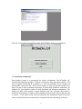
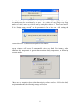
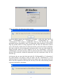
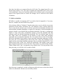
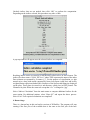
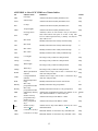
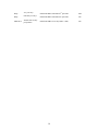
RClimDex (1.0)
User Manual
By
Xuebin Zhang and Feng Yang
Climate Research Branch
Environment Canada
Downsview, Ontario
Canada
September 10, 2004
Acknowledgement
The RClimDex is developed and maintained by Xuebin Zhang and Feng Yang at the
Climate Research Branch of Meteorological Service of Canada. Its initial development
was funded by the Canadian International Development Agency through the Canada
China Climate Change Cooperation (C5) Project. Lisa Alexander, Francis Zwiers, Byron
Gleason, David Stephenson, Albert Klan Tank, Mark New, Lucie Vincent, and Tom
Peterson made important contributions to the development and testing of the package.
Jose Luis Santos at CIIFEN helped to translate this document into Spanish. Earlier
versions of RClimDex have been used during CCl/CLIVAR ETCCDMI workshops in
Cape Town, South Africa, May 31-June 4, 2004, and in Maceio, Brazil, August 9-14,
2004. The lectures and attendees of the workshops provided very valuable suggestions for
the improvement of RClimDex.
2
TABLE OF CONTENTS
1. Introduction
2. Installation and running of R
2.1 How to install R
2.2 How to run R
3. How to use RClimDex
3.1 Loading of RClimDex
3.2 Data quality control
3.3 Calculation of Indices
4. Known bugs
5. Bug report
Appendix A:
List of Climate Indices
Appendix B:
Input Data Format
Appendix C: Indices definitions
Appendix D: Threshold and in-base period temperature indices calculation
Appendix E: R for Windows FAQ
3
1. Introduction
ClimDex is a Microsoft Excel based program that provides an easy-to-use software
package for the calculation of indices of climate extremes for monitoring and detecting
climate change. It was developed by Byron Gleason at the National Climate Data Centre
(NCDC) of NOAA, and has been used in CCl/CLIVAR workshops on climate indices
fromin 2001.
The original objective was to port ClimDex into an environment that does not depend on
a particular operating system. It was very natural to use R as our platform, since R is a
free and yet very robust and powerful software for statistical analysis and graphics. It
runs under both Windows and Unix environments. In 2003 it was discovered that the
method used for computing percentile-based temperature indices in ClimDex and other
programs resulted in inhomogeneity in the indices series. A fix to the problem requires a
bootstrap procedure that makes it almost impossible to implement in an Excel
environment. This has made it more urgent to develop this R based package.
RClimDex (1.0) is designed to provide a user friendly interface to compute indices of
climate extremes. It computes all 27 core indices recommended by the CCl/CLIVAR
Expert Team for Climate Change Detection Monitoring and Indices (ETCCDMI) as well
as some other temperature and precipitation indices with user defined thresholds. The 27
core indices include almost all the indices calculated by ClimDex (Version 1.3). This
version of RClimDex has been developed under R 1.84. It should run with R 1.84 or a
later version.
A main objective of constructing climate extremes indices is to use for climate change
monitoring and detection studies. This requires that the indices be homogenized. Data
homogenization has been planned but is not implemented in this release. Current
RClimDex only includes a simple data quality control procedure that was provided in
ClimDex. As in ClimDex, we require that data are quality controlled before the indices
can be computed. This users‟ manual provides step-by-step instructions on 1) The
installation of R and setting up the user environment, 2) Quality control of daily climate
data, 3) Calculation of the 27 core indices.
2. Installation and running of R
R is a language and environment for statistical computing and graphics. It is a GNU
implementation of the S language developed by John Chambers and colleagues at Bell
Laboratories (formerly AT&T, now Lucent Technologies). S-plus provides a commercial
implementation of the S language.
2.1 How to install R
RClimDex requires the base package of R and graphic user interface TclTk. The
installation of R involves a very simple procedure. 1) Connect to the R project website at
4
http://www.r-project.org, 2) Follow the links to download the most recent version of R
for your computer operating system from any mirror site of CRAN.
For Microsoft Windows (95, 98, 2000, and XP), download the Windows setup program.
Run that program and R will be automatically installed in your computer, with a short cut
to R on your desktop. The TclTk is included in the default installation of R 1.9.0 or later
versions. It may need to be installed separately if you are running an earlier version of R.
For Linux, download proper precompiled binaries and follow the instruction to install R.
For other unix systems, you many need to download source code and compile it yourself.
2.2 How to run R
Under the Windows environment, double click the R icon on your desktop, or launch it
through Windows “start” menu. This usually gets you into the R user interface. For some
computers, you may need to first setup an environment variable called “HOME”. See R
for Windows FAQ (Appendix E) for details if you have any problems.
Under a unix environment, just run R to give you the R console.
Exit from R by entering q() in the R console under both Windows and unix. Under
Windows, you may also click “File” menu and then “Exit”.
3. How to use RClimDex
3.1 Loading of RClimDex
Within the R consol prompt “>”, enter source(“rclimdex.r”). This will load RClimDex
into R environment. You may need to include the full path before the filename rclimdex.r.
Or you may download the most recent version from ETCCDMI web site by entering
source (“http://cccma.seos.uvic.ca/ETCCDMI/RClimDex/rclimdex.r”) if your computer
is connected to the internet. Under windows, RClimDex can also be loaded from drop
down menu. Choose the “File” from the RGui menu, and then select “Source R code”.
This will bring a new pop-up window within which you can select our R source code
“rclimdex.r” from the directory where the program was saved or type
http://cccma.seos.uvic.ca/ETCCDMI/RClimDex/rclimdex.r to download the latest version
from the web site .
5
Once the source code is successfully loaded, the RClimDex main menu will appear.
3.2. Load Data and Run QC
Data Quality Control is a prerequisite for indices calculations. The RClimDex QC
performs the following procedure: 1) Replace all missing values (currently coded as -99.9)
into an internal format that R recognizes (i.e. NA, not available), and 2) Replace all
unreasonable values into NA. Those values include a) daily precipitation amounts less
than zero and b) daily maximum temperature less than daily minimum temperature. In
addition, QC also identifies outliers in daily maximum and minimum temperature. The
outliers are daily values outside a region defined by the user. Currently, this region is
defined as the mean plus or minus n times standard deviation of the value for the day, that
is, [mean – n*std, mean+n*std]. Here std represents the standard deviation for the day
and n is an input from the user and mean is computed from the climatology of the day.
6
Select “Load Data and Run QC” from the RClimDex Menu to open a window as shown
below. This allows users to select (load) the data file from which indices are to be
computed.
The filename should be of the form “stationname.txt”. The values in the file should be of
the format described in Appendix B. In this menu, we use data from a station whose data
are stored in an ASCII file “21946.txt” for the purpose of demonstration. A pop-up
window, as shown below, will appear once the data for station 21946 are successfully
loaded.
Error messages will appear in the R console if this step has not been completed
successfully. This is usually caused by the wrong input data format. Please compare your
format with our sample data if you see such messages.
Unreasonable values are identified automatically but identification of outliers in
temperature data requires input from the user.
7
The default value for n is 3 (Criteria in the “Set Parameters for Data QC”) window, but
this number may be overwritten by the user. As a value of 3 may flag a very large
number of values, users may wish to start by setting this value to 4. There is no need to
fill in “Station name or code” as this parameter is for a later use. After setting the
parameter, click “OK” to continue.
In some slower PC‟s, this process may take a few minutes.
Pop-up windows will appear if unreasonable values are found. For instance, when
minimum daily temperature is greater than maximum daily temperature, the following
message appears.
If there are any negative values (other than missing values coded as -99.9) in the daily
precipitation amount, the following message will appear.
8
If there are outliers, the following window appears.
A pop-up window appears once the data QC is complete. At the same time, four Excel
files,
“21946tempQC.csv”,
“21946prcpQC.csv”,
“21946tepstdQC.csv”,
and
“21946indcal.csv” are created in a subdirectory called log. The first two files contain
information about unreasonable values for temperature and precipitation. The third file
flags all possible outliers in daily temperature with the dates on which those outliers
occur. The last file contains the QC‟d data and will be used for the indices calculation.
Note that, in this file, only missing values and unreasonable values are replaced with NA,
flagged possible outliers are NOT changed. For an easy visualization, 4 PDF files
containing time series plots (missing values are plotted as red dots) of daily precipitation
amount, daily maximum, minimum temperatures and daily temperature range are also
stored in log.
At this point, the user may check the data in the file “21946tepstdQC.csv” to determine if
any value marked as an outlier is really an outlier. The file “21946indcal.csv” can be
modified using Excel under Windows and any editor under Unix if any action needs to be
taken. After the completion of this step, the user may Click OK on the following window
to proceed with indices calculation.
9
Note that, the indices are computed from the QC‟d data. The original input file is not
altered in any manner. So if a user chose to modify the original data file to correct some
of the problematic values, the Load Data and Run QC procedure needs to be performed
again on the improved data set before the changes can be reflected in the indices
calculation.
3.3. Indices calculation
RClimDex is capable of computing all 27 core indices listed in Appendix A. Users may,
however, compute only those indices they require.
After selecting “Indices Calculation” from the main menu, a user is asked to set up some
parameters for the indices calculation. The “Set Parameter Values” window allows the
user to enter the first and last years of the base period for the threshold calculation, the
station latitude (Southern Hemisphere is negative) to determine in which hemisphere the
station is located, a user defined daily precipitation threshold, P (in mm), to compute the
number of days when daily precipitation amounts exceed this threshold (the Rnn
indicator), and 4 user defined temperature thresholds. The “User defined Upper Limit of
Day High” allows the calculation of the number of days when daily maximum
temperature has exceeded this threshold. The “User defined Lower Limit of Day High”
allows the calculation of the number of days when daily maximum temperature is below
this value. The “User defined Upper Limit of Day Low” allows the calculation of the
number of days when daily minimum temperature has exceeded this threshold. The “User
defined Lower Limit of Day Low” allows the calculation of the number of days when
daily minimum temperature is below this limit. These indices are called SUmm, FDmm,
TRmm, IDmm where “mm” corresponds to user defined value. This step includes some
data processing, so it will take a few seconds to finish.
Once this step is completed, a window will appear to allow the user to select their desired
indices for calculation. All indices are selected by default.
10
Uncheck indices that are not needed, then click “OK” to perform the computation.
Depending on the indices selected, this procedure may take a while.
A pop-up window will appear once the selected indices are computed.
Resulting indices series are stored in a sub-directory called indices in Excel format. The
indices files have names “21946_XXX.cvs” where XXX represents the name of the index.
Data columns are separated by a comma (“,”). For the purpose of visualization, we plot
annual series, along with trends computed by linear least square (solid line) and locally
weighted linear regression (dashed line). Statistics of the linear trend fitting are displayed
on the plots. These plots are stored in a sub-directory called plots in JPEG format. The
filenames for plots follow the same rule except that “cvs” is changed to “jpg”.
Select “Indices Calculation” from the main menu to compute additional indices for the
same station. For additional stations, select “Data QC” and repeat the above process.
Select “Exit” if all required calculations are completed.
4. Known bugs
There is a known bug in this and earlier versions of RClimDex. The program will stop
running if the first year of the available data is the same as the first year of the base
11
period. This is caused by come computation that requires data beyond the boundary of the
base period. The calculation of percentile based temperature indices is an example. One
way to avoid this problem is to add an extra record for the day (with values marked as
missing just before the beginning of the base period. For example, if base period is 19611990 and the data also starts in 1961, one may add “1960 12 31 -99.9 -99.9 -99.9” as the
first line for the input data file.
5. Bug report
Please report any bugs/errors to [email protected] with error messages and data being
used for the calculation of the indices. This will be helpful in producing a better release in
the near future. We would also appreciate your suggestions for further improvement.
12
APPENDIX A: List of ETCCDMI core Climate Indices
ID
FD0
SU25
ID0
TR20
GSL
TXx
TNx
TXn
TNn
TN10p
TX10p
TN90p
TX90p
WSDI
CSDI
DTR
RX1day
Rx5day
SDII
R10
R20
Rnn
CDD
CWD
Indicator name
Frost days
Summer days
Ice days
Tropical nights
Growing season
Length
Max Tmax
Max Tmin
Min Tmax
Min Tmin
Cool nights
Cool days
Warm nights
Warm days
Warm spell duration
indicator
Cold spell duration
indicator
Diurnal temperature
range
Max 1-day
precipitation amount
Max 5-day
precipitation amount
Simple daily intensity
index
Number of heavy
precipitation days
Number of very
heavy precipitation
days
Number of days
above nn mm
Consecutive dry days
Consecutive wet days
Definitions
UNITS
Annual count when TN(daily minimum)<0ºC
Days
Annual count when TX(daily maximum)>25ºC
Days
Annual count when TX(daily maximum)<0ºC
Days
Annual count when TN(daily minimum)>20ºC
st
st
Days
th
Annual (1st Jan to 31 Dec in NH, 1 July to 30 June in
SH) count between first span of at least 6 days with
TG>5ºC and first span after July 1 (January 1 in SH) of 6
days with TG<5ºC
Days
Monthly maximum value of daily maximum temp
ºC
Monthly maximum value of daily minimum temp
ºC
Monthly minimum value of daily maximum temp
ºC
Monthly minimum value of daily minimum temp
ºC
Percentage of days when TN<10th percentile
Days
Percentage of days when TX<10th percentile
Days
Percentage of days when TN>90th percentile
Days
Percentage of days when TX>90th percentile
Days
Annual count of days with at least 6 consecutive days
when TX>90th percentile
Annual count of days with at least 6 consecutive days
when TN<10th percentile
Days
Days
Monthly mean difference between TX and TN
ºC
Monthly maximum 1-day precipitation
Mm
Monthly maximum consecutive 5-day precipitation
Mm
Annual total precipitation divided by the number of wet
days (defined as PRCP>=1.0mm) in the year
Mm/da
y
Annual count of days when PRCP>=10mm
Days
Annual count of days when PRCP>=20mm
Days
Annual count of days when PRCP>=nn mm, nn is user
defined threshold
Days
Maximum number of consecutive days with RR<1mm
Days
Maximum number of consecutive days with RR>=1mm
Days
13
R95p
R99p
PRCPTOT
Very wet days
Annual total PRCP when RR>95th percentile
Mm
Extremely wet days
Annual total PRCP when RR>99th percentile
mm
Annual total PRCP in wet days (RR>=1mm)
mm
Annual total wet-day
precipitation
14
APPENDIX B: Input Data Format
All of the data files that are read or written are in list formatted format. The exception is
the very first data file that is processed in the “ Quality Control” step. This input data file
has several requirements:
1.
ASCII text file
2.
Columns as following sequences: Year, Month, Day, PRCP, TMAX, TMIN.
(NOTE: PRCP units = millimeters and Temperature units= degrees Celsius)
3.
The format as described above must be space delimited (e.g. each element
separated by one or more spaces).
4.
For data records, missing data must be coded as -99.9; data records must be in
calendar date order. Missing dates allowed.
Example data Format for the initial data file (e.g. used in the „Quality Control‟ step):
1901
1901
1901
1901
1901
1
1
1
1
1
1
2
3
4
7
-99.9
-99.9
-99.9
-99.9
-99.9
-3.1
-1.3
-0.5
-1
-1.8
-6.8
-3.6
-7.9
-9.1
-8.4
15
APPENDIX C: Indices definitions
Definitions for indicators listed in Appendix A. For practical reasons, in this version of
the software, not all indices are calculated on a monthly basis. Monthly indices are
calculated if no more than 3 days are missing in a month, while annual values are
calculated if no more than 15 days are missing in a year. No annual value will be
calculated if any one month‟s data are missing. For threshold indices, a threshold is
calculated if at least 70% of data are present. For spell duration indicators (marked with a
*), a spell can continue into the next year and is counted against the year in which the
spell ends e.g. a cold spell (CSDI) in the Northern Hemisphere beginning on 31st
December 2000 and ending on 6th January 2001 is counted towards the total number of
cold spells in 2001.
1. FD0
Let Tnij be the daily minimum temperature on day i in period j . Count the number of
days where:
Tnij  0C
2. SU25
Let Txij be the daily maximum temperature on day i period j . Count the number of days
where:
Txij  25C
3. ID0
Let Txij be the daily maximum temperature on day i in period j . Count the number of
days where:
Txij  0C
4. TR20
Let Tnij be the daily minimum temperature on day i in period j . Count the number of
days where:
Tnij  20C
5. GSL
16
Let Tij be the mean temperature on day i in period j . Count the number of days between
the first occurrence of at least 6 consecutive days with:
Tij  5o C
and the first occurrence after 1st July (1st January in SH) of at least 6 consecutive days
with:
Tij  5o C
6. TXx
Let Txkj be the daily maximum temperatures in month k , period j . The maximum daily
maximum temperature each month is then:TXxkj  max(Txkj )
7. TNx
Let Tnkj be the daily minimum temperatures in month k , period j . The maximum daily
minimum temperature each month is then:TNxkj  max(Tnkj )
8. TXn
Let Txkj be the daily maximum temperatures in month k , period j . The minimum daily
maximum temperature each month is then:TXnkj  min(Txkj )
9. TNn
Let Tnkj be the daily minimum temperatures in month k , period j . The minimum daily
minimum temperature each month is then:TNnkj  min(Tnkj )
10. Tn10p
Let Tnij be the daily minimum temperature on day i in period j and let Tnin10 be the
calendar day 10th percentile centred on a 5-day window (calculated using method from
Appendix D). The percentage of time is determined where:
17
Tnij  Tnin10
11. Tx10p
Let Txij be the daily maximum temperature on day i in period j and let Txin10 be the
calendar day 10th percentile centred on a 5-day window (calculated using method from
Appendix D). The percentage of time is determined where:
Txij  Txin10
12. Tn90p
Let Tnij be the daily minimum temperature on day i in period j and let Tnin90 be the
calendar day 90th percentile centred on a 5-day window (calculated using method from
Appendix D). The percentage of time is determined where:
Tnij  Tnin90
13. Tx90p
Let Txij be the daily maximum temperature on day i in period j and let Txin90 be the
calendar day 90th percentile centred on a 5-day window (calculated using method from
Appendix D). The percentage of time is determined where:
Txij  Txin90
14. WSDI*
Let Txij be the daily maximum temperature on day i in period j and let Txin90 be the
calendar day 90th percentile centred on a 5-day window (calculated using method from
Appendix D). Then the number of days per period is summed where, in intervals of at
least 6 consecutive days:-
Txij  Txin90
15. CSDI*
Let Tnij be the daily minimum temperature at day i in period j and let Txin10 be the
calendar day 10th percentile centred on a 5-day window (calculated using the method
from Appendix D). Then the number of days per period is summed where, in intervals of
at least 6 consecutive days:-
Tnij  Tnin10
16. DTR
18
Let Txij and Tnij be the daily maximum and minimum temperature respectively on day
i in period j . If I represents the number of days in j , then:
I
 Tx
ij
DTRj 
 Tnij 
i 1
I
17. RX1day
Let RRij be the daily precipitation amount on day i in period j . Then maximum 1-day
values for period j are:
Rx1dayj  max( RRij )
18. Rx5day
Let RRkj be the precipitation amount for the 5-day interval ending k , period j . Then
maximum 5-day values for period j are:
Rx5dayj  max( RRkj )
19. SDII
Let RRwj be the daily precipitation amount on wet days, w( RR  1mm) in period j . If
W represents number of wet days in j , then:
W
SDIIj 
 RRwj
w1
W
20. R10
Let RRij be the daily precipitation amount on day i in period j . Count the number of
days where:
RRij  10mm
21. R20
Let RRij be the daily precipitation amount on day i in period j . Count the number of
days where:
RRij  20mm
19
22. Rnn
Let RRij be the daily precipitation amount on day i in period j . If nn represents any
reasonable daily precipitation value then, count the number of days where:
RRij  nnmm
23. CDD*
Let RRij be the daily precipitation amount on day i in period j . Count the largest number
of consecutive days where:
RRij  1mm
24. CWD*
Let RRij be the daily precipitation amount on day i in period j . Count the largest number
of consecutive days where:
RRij  1mm
25. R95pTOT
Let RRwj be the daily precipitation amount on a wet day w( RR  1.0mm) in period j and
let RRwn95 be the 95th percentile of precipitation on wet days in the 1961-1990 period. If
W represents the number of wet days in the period, then:
W
R95 pj   RRwj where RRwj  RRwn95
w=1
26. R99p
Let RRwj be the daily precipitation amount on a wet day w( RR  1.0mm) in period j and
let RRwn99 be the 99th percentile of precipitation on wet days in the 1961-1990 period. If
W represents number of wet days in the period, then:
W
R99 pj   RRwj where RRwj  RRwn99
w=1
27. PRCPTOT
Let RRij be the daily precipitation amount on day i in period j . If I represents the
number of days in j , then
20
I
PRCPTOTj   RRij
i 1
21
Appendix D : Threshold estimation and base period temperature indices calculation
Empirical quantile estimation:
The quantile of a distribution is defined as
Q ( p )  F 1 ( p )  inf{ x : F ( x )  p} , 1<p<1,
where F(x) is the distribution function. Let { X ( a ) ,..., X ( n ) } denote the order statistics of
{ X 1 ,..., X n } (i.e. sorted values of {X}), and let Qˆ i ( p) denote the ith sample quantile
definition. The sample quantiles can be generally written as
Qˆ i ( p)  (1   ) X ( j )  X ( j 1) .
Hyndman and Fan (1996) suggest a formula to obtain medium un-biased estimate of the
quantile by letting j  int( p * n  (1  p) / 3)) and letting   p * n  (1  p) / 3  j , where
int(u) is the largest integer not greater than u. The empirical quantile is set to the smallest
or largest value in the sample when j<1 or j> n respectively. That is, quantile estimates
corresponding to p<1/(n+1) are set to the smallest value in the sample, and those
corresponding to p>n/(n+1) are set to the largest value in the sample.
Bootstrap procedure for the estimation of exceedance rate for the base period:
It is not possible to make an exact estimate of the thresholds due to sampling uncertainty.
To provide temporally consistent estimate of exceedance rate throughout the base period
and out-of-base period, we adapt the following procedure (Zhang et al. 2004) to estimate
exceedance rate for the base period.
a) The 30-year base period is divided into one “out-of-base” year, the year for which
exceedance is to be estimated, and a “base-period” consisting the remaining of 29
years from which the thresholds would be estimated.
b) A 30-year block of data is constructed by using the 29 year “base-period” data set
and adding an additional year of data from the “base-period" (i.e., one of the years
in the “base-period” is repeated). This constructed 30-year block is used to
estimate thresholds.
c) The “out-of-base” year is then compared with these thresholds and the exceedance
rate for the “out-of-base” year is obtained.
d) Steps (b) and (c) are repeated for an additional 28 times, by repeating each of the
remaining 28 in-base years in turn to construct the 30-year block.
e) The final index for the “out-of-base” year is obtained by averaging the 29
estimates obtained from steps (b), (c) and (d).
Reference:
Hyndman, R.J., and Y. Fan, 1996: Sample quantiles in statistical packages. The American
Statistician, 50, 361-367.
22
Zhang, X., G. Hegerl, F.W. Zwiers, and J. Kenyon, 2004: Avoiding inhomogeneity in
percentile-based indices of temperature extremes. J. Climate, submitted.
Appendix E: R for Windows FAQ
23