Download Bayesian Inference Using WBDev: A Tutorial for

A WBDEV TUTORIAL
5
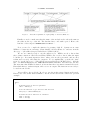
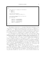
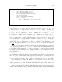
The twiddles symbol (∼) means “is distributed as”. Because we use a Uniform distribution between 0 and 1 as a prior on the rate parameter θ, we write theta ∼ dunif(0,1).
This indicates that, a priori, each value of θ is equally likely. Furthermore, k is Binomially
distributed with parameters θ and n (i.e., k ∼ dbin(theta,n)). Note that dunif and
dbin are two of the predefined distributions in WinBUGS. All the distributions that are
predefined in WinBUGS are listed in the distributions section in the WinBUGS manual,
which can be accessed by clicking the help menu and selecting User manual (or by pressing
F1). The hash symbol (#) is used for comments. The lines starting with this symbol are
not executed by WinBUGS.
Copy the text into an empty file and save it as “model rateproblemfunction.txt” in the
directory from where you want to work. There are now various ways in which to proceed.
One way is to work from within WinBUGS; another way is to control WinBUGS by calling
it from a more general purpose program. Here, we use the statistical programming language
R5 to call WinBUGS, but widely–used alternative research programming environments such
as MATLAB are also available (Lee & Wagenmakers, 2009).
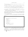
A rate problem: the R script. The next step is to construct an R–script to call
Blackbox from R.6 When you run the script “Rscript RateProblemFunction.R”, WinBUGS
starts, the MCMC sampling is conducted, WinBUGS closes, and you return to R. The
object that WinBUGS has returned to R is called “rateproblem”, and this object contains
all the information about the Bayesian inference for θ.
In particular, the “rateproblem” object contains a single sequence of consecutive
draws from the posterior distribution of θ, a sequence that is generally known as an MCMC
chain. Inspection of the MCMC chain is an important part of the analysis because valid
inference requires that the chain has converged, meaning that the samples have been drawn
from the posterior distribution.
Convergence problems can occur in a variety of situations. One source of non–
convergence can be in the data. For example, there may be too little data available, or
the data may not be in agreement with the model that was used. However, lack of convergence can also originate from the model itself. For example, the model may have too
many parameters, or it may have parameters that are highly correlated. Another situation
in which the MCMC chain might not converge is when the priors are unrealistic.
Because lack of convergence can lead to invalid results, it is important to check
whether the MCMC chains have converged. One way to check this is to run multiple
chains with overdispersed starting values. Despite the differing starting values, the chains
should be indistinguishable from each other after enough samples have been drawn. Moreover, these chains should all have the same, constant mean. Another visual test is that
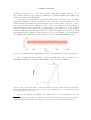
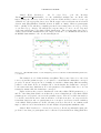
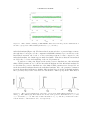
when an MCMC chain has converged, each chain should look like a “fat hairy caterpillar”
(see for instance Figure 4). This should happen when the subsequent draws are (relatively)
independent and when a chain consists of many samples.
Apart from a visual inspection of the chains, more formal tests for convergence exist
as well. One often–used method is the Gelman and Rubin (1992) R̂ statistic that compares
the between–chain variance to the within–chain variance. When the chain has converged,
5
6
R is, at the time of writing, freely available from: http://www.r-project.org/.
All the scripts can be found on the website of the first author: http://www.ruudwetzels.com.