Download Handout - The Ohio State University

WinBUGS Tutorial Outline
August 4, 2005
Authors: Ed Merkle & Trisha Van Zandt
• WinBUGS overview
• Description of Example Data
• Example 1: Confidence in Signal Detection
• Example 2: Mean RT Model
• Example 3: Estimating RT Distributions
• Conclusions/Things to Remember
1
WinBUGS Overview
WinBUGS is a computer program aimed at making MCMC
available to applied researchers such as mathematical psychologists.
Its interface is fairly easy to use, and it can also be called from
programs such as R. WinBUGS is free and can be found on the
website:
http://www.mrc-bsu.cam.ac.uk/bugs/winbugs/contents.shtml
To obtain full, unrestricted use, you have to fill out a registration
form and get an access key. This is only so that the authors of
WinBUGS can prove they spent their grant money on developing a
useful product.
Linux users can obtain the OpenBUGS program, found at:
http://mathstat.helsinki.fi/openbugs/
This workshop will focus exclusively on the WinBUGS program.
2
What Does WinBUGS Do?
Given a likelihood and prior distribution, the aim of WinBUGS is
to sample model parameters from their posterior distribution. After
the parameters have been sampled for many iterations, parameter
estimates can be obtained and inferences can be made. A good
introduction to the program can be found in Sheu and O’Curry
(1998).
The exact sampling method used by WinBUGS varies for different
types of models. In the simplest case, a conjugate prior distribution
is used with a standard likelihood to yield a posterior distribution
from which parameters may be directly sampled. In more
complicated cases, the form of the posterior distribution does not
allow for direct sampling. Instead, some form of Gibbs sampling or
Metropolis-Hastings sampling is used to sample from the posterior
distribution. These techniques generally work by first sampling
from a known distribution that is similar in shape to the posterior
distribution and then accepting the sample with some probability.
To learn more about these sampling schemes, see the “MCMC
methods” section (and the cited references) in the Introductory
chapter of the WinBUGS user manual that (electronically) comes
with the program.
3
General Program Layout
For a given project, three files are used:
1. A program file containing the model specification.
2. A data file containing the data in a specific (slightly strange)
format.
3. A file containing starting values for model parameters
(optional).
File 3 is optional because WinBUGS can generate its own starting
values. There is no guarantee that the generated starting values are
good starting values, though.
If you are familiar with R/SPlus, you are at both an advantage and
a disadvantage in learning WinBUGS. You are at an advantage
because the model specification in WinBUGS uses commands that
are highly similar to R/SPlus. You are at a disadvantage because
WinBUGS doesn’t have all the commands that R/SPlus has; thus,
you get errors when you try to use undefined R/SPlus commands.
4
Model Specification
In general, model specification in WinBUGS proceeds by defining
distributions for the data and associated parameters. Most
commonly-used distributions are already defined in WinBUGS, so
that the model specification consists of calling these distributions.
Distributions are assigned using the ~ operator, and relationships
among variables can be defined using the <- operator.
Prior distributions on the model parameters are also given in the
model specification file, using the ~ operator.
For example, consider a simple signal detection model. For each
trial, we observe a participant’s response (0 or 1) along with the
correct response. We can use the following model specification to
estimate the mean difference and threshold of the SDT model:
5
model
{
# x is vector of observed responses (1/2)
# y is vector of correct response
# Define x as categorical with probability of response
# determined by SDT model.
for (i in 1:N){
x[i] ~ dcat(p[i,])
# Define SDT probabilities, assuming variance of 0.5
p[i,1] <- phi((c - mu*y[i])/0.5)
p[i,2] <- 1 - p[i,1]
}
# Define prior distributions on model parameters.
mu ~ dnorm(0,0.0001)
c ~ dnorm(0,0.0001)
}
list(mu=0.5,c=0.25)
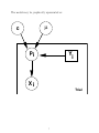
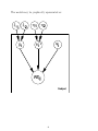
6
The model may be graphically represented as:
µ
c
pi
Yi
Xi
Trial
7
Data Specification
Getting the data into WinBUGS can be a nuisance. There are two
different formats that the program accepts: R/Splus format
(hereafter referred to simply as R format) and rectangular format.
As the name suggests, the R or Splus programs can be used to get
your data into R/Splus format. Assuming your data are in vectors
x, y, and z within R, you can enter a command similar to:
dput(list(x=x,y=y,z=z), file=‘‘mydata.dat’’).
This command puts your data in the proper format and writes to
the file “mydata.dat”. Note that, when your data are in matrix
format, the dput command doesn’t put your data in the exact
format required by WinBUGS. WinBUGS doesn’t always like the
dimensions of R matrices, but the WinBUGS help files clearly tell
you how to solve this problem. Furthermore, for matrices, we have
found that R doesn’t add the required “.Data=” command before
the matrix entries.
8
The rectangular data format can be used if you have a text file
containing each of your variables in a separate column. For vectors
x, y, and z, the rectangular data file would look like:
x[]
y[]
z[]
4
5
6
7
8
9
......
20
21
22
END
Note that brackets are needed after each variable name and “END”
is needed at the end of the data file.
For the simple signal detection example, the data file (in R format)
would look like:
list(x = c(1,2,1,1,...), y = c(0,1,0,1,...))
The x variable must be coded as 1/2 instead of 0/1 to use the
categorical distribution (dcat) in WinBUGS. In general, the
categories of a categorical variable must start at 1 instead of 0.
9
Specification of Starting Values
As described earlier, WinBUGS does have the capability of defining
starting values for free parameters. These starting values are not
always good ones. If starting values are bad, the program can hang,
yield inaccurate results, or freeze. To specify your own starting
values, you can create a new file that looks similar to the data file
that has specific values for model parameters.
For the signal detection example, the free parameters are “mu” and
“thresh”. We might want to specify the starting value of mu to be
0.5 and the starting value of thresh to be 0.25. This would look like:
list(mu = 0.5, threshold = 0.25)
10
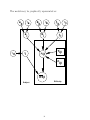
Initializing the Model
Now that the model, data, and starting values have been specified,
we can think about running the program. Before actually running
the analysis, you must submit the model specification and data to
WinBUGS. If the syntax is good, then WinBUGS will let you run
the analysis. If the syntax is bad, WinBUGS often gives you a hint
about where the problem is.
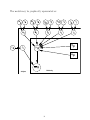
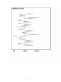
It is generally easiest to arrange windows within WinBUGS in a
specific manner. One possible arrangement is shown on the
following page. Once your windows are arranged, click on
“Specification...” under “Model” on the main menu bar. This will
bring up the Model Specification Tool, which is what allows you to
enter your model into WinBUGS.
After bringing up the model specification tool, highlight the word
“model” at the top of your model specification file. Then click
“check model” on the model specification tool. If your syntax is
good, you will see a “model is syntactically correct” message in the
lower left corner of the WinBUGS window (the message is small
and easy to miss). If your syntax is bad, you will see a message in
the lower left corner telling you so.
11
12
Assuming your model is syntactically correct, highlight the word
“list” at the top of your data file and click “load data” on the
Model Specification Tool. If your data are in the correct format,
you will see a “data loaded” message in the lower left corner. Next,
click “compile” on the model specification tool. The compiler can
find some errors in your model and/or data that were not
previously caught. If the model/data are compiled successfully, you
will see a “model compiled” message.
Finally, after compiling the model, you must obtain starting values.
If you have provided them, highlight the word “list” at the top of
your starting values and click “load inits”. If you want WinBUGS
to generate starting values, simply click “gen inits” on the Model
Specification Tool. Once you see the message “model is initialized”
in the lower left corner, you are ready to get your simulation on!
13
Running the Simulation
Now that the model is initialized, click “Samples...” off of the
inference menu to bring up the Sample Monitor Tool. It is here
that you tell WinBUGS which parameters you are interested in
monitoring. This is accomplished by typing each parameter name
in the “node” box and clicking “set”. For the signal detection
example, we are interested in monitoring the mu and thresh
parameters. So we type both of these variables and click “set” after
each one.
Now we are ready to begin the simulation. Click “Update...” from
the Model menu. Type the number of iterations you wish to
simulate in the “updates” box and click on the update button. The
program is running if you see the number in the “iteration” box
increasing. If you have waited a long time and nothing happens, it
is possible that the program has frozen. Changing the parameter
starting values is one remedy that sometimes solves this problem.
14
Assessing Convergence
As stated before, in the absence of conjugate prior distributions,
WinBUGS uses sampling methods. These sampling methods
typically guarantee that, under regularity conditions, the resulting
sample converges to the posterior distribution of interest. Thus,
before we summarize simulated parameters, we must ensure that
the chains have converged.
Time series plots (iteration number on x-axis and parameter value
on y-axis) are commonly used to assess convergence. If the plot
looks like a horizontal band, with no long upward or downward
trends, then we have evidence that the chain has converged.
Autocorrelation plots can also help here: high autocorrelations in
parameter chains often signify a model that is slow to converge.
15
Finally, WinBUGS provides the Gelman-Rubin statistic for
assessing convergence. For a given parameter, this statistic assesses
the variability within parallel chains as compared to variability
between parallel chains. The model is judged to have converged if
the ratio of between to within variability is close to 1. Plots of this
statistic can be obtained in WinBUGS by clicking the “bgr diag”
button. The green line represents the between variability, the blue
line represents the within variability, and the red line represents the
ratio. Evidence for convergence comes from the red line being close
to 1 on the y-axis and from the blue and green lines being stable
(horizontal) across the width of the plot.
Parameter values that have been sampled at the beginning of the
simulation are typically discarded so that the chain can “burn in”,
or converge to its stationary distribution. Large, conservative
burn-in periods are generally preferable to shorter burn-in periods.
16
Summarizing Results
After the simulation has completed, we can examine results using
the Sample Monitor Tool. A burn-in period can be specified by
changing the 1 in the “beg” box to a larger number. Furthermore,
different percentiles of interest may be highlighted for a given
variable. Highlight one of the variables on the drop-down node
menu and click “stats”. This gives you some summary statistics
about the chosen parameter. The “history” and “auto cor” buttons
provide plots that are helpful for monitoring convergence, and the
“coda” button provides a list of all simulated values for the selected
parameter.
There are other monitoring tools that can be found on the Inference
menu. The Comparison Tool can plot observed vs. predicted data,
and it can also provide summary plots for parameter vectors. The
Summary and Rank Monitor Tools are similar to the Sample
Monitor Tool, but they reduce the storage requirements (which may
be helpful for complicated models). The DIC tool provides a model
comparison measure; more information about it can be found in the
WinBUGS help files and website.
17
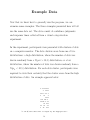
Example Data
Now that we know how to generally run the program, we can
examine some examples. The three examples presented here will all
use the same data set. The data consist of confidence judgments
and response times collected from a visual categorization
experiment.
In the experiment, participants were presented with clusters of dots
on a computer monitor. The dots clusters arose from one of two
distributions: a high distribution, where the number of dots was
drawn randomly from a N(µH > 50,5) distribution, or a low
distribution, where the number of dots was drawn randomly from a
N(µL < 50,5) distribution. For each dots cluster, participants were
required to state their certainty that the cluster arose from the high
distribution of dots. An example appears below.
* ** *****
* ****
*** * ** *
*
**
*
****
*** *** *
***** * **
** ***
** ** **
* ** ***
‘‘I am X% sure that this is output by the high process’’
18
Each trial consisted of participants giving their certainty that a
specific cluster of dots arose from the high distribution. For each
trial, the following data were obtained:
• Confidence: The participant’s confidence response, from 5% to
95% in increments of 10%.
• Correct Distribution: The true distribution from which the
cluster of dots arose.
• Condition: An easy condition consisted of µH = 55 and
µL = 45; a hard condition consisted of µH = 53 and µL = 47.
• Implied Response: The participant’s implied choice based on
her confidence judgment.
• Number of Dots: The number of dots in a specific dots cluster.
• RT: The participant’s confidence response time in msec.
Portions of these data will be used in the WinBUGS examples that
follow.
19
Disclaimer
In the examples that follow, we estimate relatively simple models
using relatively simple data sets. The models are intended to
introduce WinBUGS to a general audience; they are not intended
to be optimal for the given data sets. Furthermore, we do not
recommend blind application of these models to future data sets.
20
Example 1:
Confidence in Signal Detection
There are many ways that we might model choice confidence, one of
which arises from a signal detection framework. Such a framework
has been previously developed by Ferrell and McGoey (1980). The
idea is that partitions are placed on the signal and noise
distributions of a signal detection model such that confidence
depends on which partitions a particular stimulus falls between. For
use with the current data, this idea may be graphically represented
as:
5% 15% 25% 35% 45% 55% 65% 75% 85% 95%
Number of Dots
21
Mathematically, let x be an n × 1 vector of confidence judgments
across trials and participants. For the experimental data described
above, x is an ordinal variable with 10 categories (5%, 15%, . . . ,
95%). Let γ be an 11 × 1 vector of partitions on the high and low
distributions of dots (e.g., signal and noise distributions in a
standard signal detection framework). Given that the dots arose
from distribution k (k =(Low,High)), the probability that xi falls in
category j is given as:
Φ((γj − µk )/s) − Φ((γj−1 − µk )/s),
(1)
where Φ represents the standard normal cumulative distribution
function, s is the common standard deviation of the high and low
dots distributions, and γ1 and γ11 are set at −∞ and +∞,
respectively.
We will use data only from the easy condition of the experiment;
thus, we can set the µk and s parameters equal to the mean and sd
parameters from the distributions of dots that were used in the easy
condition. That is, we set µL = 45, µH = 55, and s = 5. We are
interested in estimating the threshold parameters γ2, γ3, . . . , γ10 in
WinBUGS.
22
Model Specification
The model may be coded into WinBUGS in the following manner.
model
{
# y is vector of distribution from which dots arose
# x is vector of raw confidence data
mu[1] <- 45
mu[2] <- 55
for (i in 1:2){
p[i,1] <- phi((gamm[1] - mu[i])/5)
for (j in 2:9){
p[i,j] <- phi((gamm[j]-mu[i])/5) - phi((gamm[j-1]-mu[i])/5)
}
p[i,10] <- 1 - phi((gamm[9] - mu[i])/5)
}
for (k in 1:N){
x[k] ~ dcat(p[y[k]+1,])
}
gamm[1] ~
for (j in
gamm[j]
}
gamm[9] ~
}
dnorm(50, 1.0E-06)I(,gamm[2])
2:8){
~ dnorm(50, 1.0E-06)I(gamm[j-1],gamm[j+1])
dnorm(50, 1.0E-06)I(gamm[8],)
23
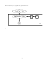
The model may be graphically represented as:
γ , γ , γ , ... , γ
0 1 2
9
pi0, pi1, pi2, ... , pi9
X ij
µ
i
Yi
Trial
,
24
Notes on the Model Specification
• Confidence judgments are modeled as categorical variables,
with probabilities based on the threshold parameters and the
distribution from which the dots arose.
• The γ vector is of length 9 instead of 11, as it was when the
model was initially described. This is because WinBUGS did
not like the 11 × 1 vector γ containing the fixed parameters
γ1 = −∞ and γ11 = +∞.
• Ordering of the parameters in γ is controlled by the prior
distributions. Each parameter’s prior distribution is essentially
flat and is censored by the other threshold parameters
surrounding it using the “I(,)” specification. For another
example on the use of ordered thresolds, see the “Inhalers”
example included with WinBUGS.
• Sampling from this model is slow; it takes a couple minutes per
1000 iterations. It is thought that the censoring causes this
delay.
25
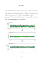
Results
Using the Model Specification Tool, 3 parameter chains were set up
to be sampled for 1500 iterations each. The first 500 iterations were
discarded from each chain, leaving a total sample of 3000 to
summarize.
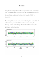
The mixing of the chains can be examined using time series plots of
each simulated parameter. These can be accessed using the
“history” button on the Sample Monitor Tool. For example, the
plots for γ1 and γ2 look like:
26
Convergence of the chains can be monitored using the time series
plots, autocorrelation plots (“auto cor” on the Sample Monitor
Tool), and Gelman-Rubin statistic (“bgr diag” on the Sample
Monitor Tool). These tools help to convince us that the current
model has converged. Next, the model parameters can be
summarized using the “stats” button on the Sample Monitor Tool.
Results for our sample of 3000 are:
27
The statistics box provides us with means, standard deviations, and
confidence intervals of the model parameters. If we believe this
model, the parameters can be interpreted as the cutoff numbers of
dots that participants used to determine confidence judgments. For
example, participants would give a “55%” judgment when the
number of dots was between 49.02 and 50.45 (e.g., when the
number of dots was equal to 49 or 50). Interestingly, this model
indicates that participants required more evidence before giving a
“5%” response than they did before giving a “95%” response.
While we obtained overall parameter estimates in this example, it
may be more interesting to obtain cutoff parameter estimates for
each individual participant. The idea of obtaining subject-level
parameters is expanded upon in the following example.
28
Example 2:
A Model for Mean RT
We can use our experimental data to examine the relationship
between response time and difficulty. You may recall that, for each
trial in our experiment, we recorded the number of dots that were
output to the computer screen. Because the experiment required
participants to distinguish between two distributions of dots, the
number of dots presented on each trial can be used as a measure of
difficulty. In general, response time decreases with difficulty.
The distributions of dots were always symmetric around 50: for the
easy condition, µL = 45 and µH = 55, and for the hard condition,
µL = 47 and µH = 53. Thus, presentation of exactly 50 dots on the
screen would be the most difficult stimulus to distinguish. As the
number of dots moves away from 50, the task gets easier.
29
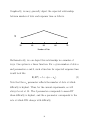
Graphically, we may generally depict the expected relationship
RT
between number of dots and response time as follows.
30
40
50
60
70
Number of Dots
Mathematically, we can depict this relationship in a number of
ways. One option is a linear function. For a given number of dots n
and parameters a and b, such a function for expected response time
would look like:
E(RT ) = b + a|n − n0|.
(2)
Note that the n0 parameter reflects the number of dots at which
difficulty is highest. Thus, for the current experiments, n0 will
always be set at 50. The b parameter corresponds to mean RT
when difficulty is highest, and the a parameter corresponds to the
rate at which RTs change with difficulty.
30
One problem with the linear function is that it never asymptotes;
as the task gets easier and easier, response times decrease to zero.
To correct this problem, a second way of modeling the relationship
between RT and task difficulty involves the exponential function.
For a given number of dots n and parameters a, b, and λ, we can
take:
E(RT ) = b + a exp(−λ|n − n0|).
(3)
The parameter interpretations here are not as straightforward as
they were above. The b parameter is an intercept term, but the
mean RT at the highest difficulty level equals a + b. The a
parameter plays a role in both the rate of change and the intercept,
and the λ parameter affects the rate at which RT s change as a
function of difficulty.
31
To model the distributions of individual participants, the expected
response times can be further modified. That is, for modeling
individual i’s RT on trial j using the linear function, we might take:
E(RTij ) = bi + (ai + βiI(h))|nij − 50|,
(4)
where I(h) equals 1 when the stimulus is hard and 0 when the
stimulus is easy. Such a function allows us to both model
participant-level parameters and incorporate difficulty effects on
RT.
A similar exponential function might look like:
E(RTij ) = bi + (ai + βiI(h)) exp(−(λi + γiI(h))|nij − 50|).
(5)
We arrive at a model for RT as a function of difficulty by assuming
that RTij ∼ N (E(RTij ), τi), where the expectation is defined using
one of the above functions and τi is estimated from the data.
32
Linear Model Specification
We may code the linear model into WinBUGS as follows (starting
values are listed at the bottom).
model
{
for (i in 1:N) {
for (j in 1:C) {
for (l in 1:D) {
mu[i,j,l] <- b[i] + (a[i] + hard[i,j,l]*beta[i]) *
(dots[i,j,l]-50.0)
RT[i,j,l] ~ dnorm(mu[i,j,l], tau[i])
}
}
b[i] ~ dnorm(b.c,tau.b)
a[i] ~ dnorm(a.c,tau.a)
beta[i] ~ dnorm(beta.c,tau.beta)
tau[i] ~ dgamma(1.0,tau.0)
}
b.c ~ dgamma(1.0,1.0E-3)
a.c ~ dnorm(0.0,1.0E-3)
beta.c ~ dnorm(0.0,1.0E-3)
tau.b ~ dgamma(1.0,1.0E-3)
tau.a ~ dgamma(1.0,1.0E-3)
tau.beta ~ dgamma(1.0,1.0E-3)
tau.0 ~ dgamma(1.0,1.0E-3)
}
list(
b.c=5.0,a.c=1.0,beta.c=-0.5,
tau.b=1.0,tau.a=1.0,tau.beta=1.0,
tau.0=1.0
)
33
The model may be graphically represented as:
a
τa
0
a
τ0
i
τ
i
b
0
τb
b
i
µijl
β0
βi
Yijl
n
ijl
RTijl
Difficulty
Subject
34
τβ
Notes on the Model Specification
• Number of dots have been divided into D=6 groups of
difficulty. For example, group 1 contains RTs for 48-52 dots,
group 2 contains RTs for 53-57 dots (and for 43-47 dots), . . .,
group 6 contains RTs for 73-77 dots (and for 23-27 dots).
Examination of the data file should make this clearer.
• There are C=2 difficulty conditions (hard/easy) that are
referred to in the specification.
• This specification references matrices of 3 dimensions. That is,
mu[i,j,l] corresponds to the expected RT for subject i in
difficulty condition j in dots group l.
• Not all participants have been observed at extreme numbers of
dots. Thus, there are some missing values in the response
variable RT (denoted by NA). WinBUGS can handle these
missing values.
• Sampling from this model is very fast.
35
Results
Using the Model Specification Tool, 3 parameter chains were set up
to be sampled for 1500 iterations each. The first 500 iterations from
each chain were discarded, leaving a total sample of 3000 to
summarize. Time series plots display good mixing of the chains (all
other plots/measures indicate convergence):
36
Based on the simulated parameter chains, 95% credibility intervals
for b.c, a.c, and beta.c are (6.66,6.86), (-0.002,0.008), and
(-0.019,-0.014), respectively. This provides evidence that RTs
generally decrease with difficulty in the hard condition but not in
the easy condition. Participants always completed the easy
condition before the hard condition in the experiment, so practice
effects may contribute to this atypical result.
Other results of interest include the participant-level parameter
estimates. These could be used, for example, to study individual
differences or to exclude participants that did not follow directions.
37
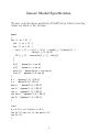
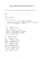
Exponential Model Specification
We may code the exponential model into WinBUGS as follows.
model
{
for (i in 1:N) {
for (j in 1:C) {
for (l in 1:D) {
mu[i,j,l] <- b[i] + (a[i] + hard[i,j,l]*beta[i]) *
exp(-(dots[i,j,l]-50.0)*(lambda[i]+hard[i,j,l]*gamma[i]))
RT[i,j,l] ~ dnorm(mu[i,j,l], tau[i])
}
}
b[i] ~ dnorm(b.c,tau.b)
a[i] ~ dnorm(a.c,tau.a)
beta[i] ~ dnorm(beta.c,tau.beta)
lambda[i] ~ dnorm(lambda.c,tau.lambda)
gamma[i] ~ dnorm(gamma.c,tau.gamma)
tau[i] ~ dgamma(1.0,tau.0)
}
b.c ~ dgamma(0.1,0.01)
a.c ~ dnorm(0.0,1.0E-3)
beta.c ~ dnorm(0.0,1.0E-3)
lambda.c ~ dnorm(0.0,1.0E-3)
gamma.c ~ dnorm(0.0,0.01)
tau.b ~ dgamma(0.15,0.01)
tau.a ~ dgamma(1.0,0.01)
tau.beta ~ dgamma(0.3,0.01)
tau.lambda ~ dgamma(4.0,0.01)
tau.gamma ~ dgamma(3.0,0.01)
tau.0 ~ dgamma(1.0,1.0)
}
38
The model may be graphically represented as:
a
τa
0
a
τ0
i
τ
i
b
0
τb
τβ
β0
b
i
βi
λ0
τλ
λi
γ
0
τγ
γi
Yijl
µijl
n
ijl
RTijl
Difficulty
Subject
39
Starting values for the exponential model are listed below.
list(
b.c=5.0,a.c=1.0,beta.c=-0.5,lambda.c=0.0,gamma.c=0.0,
tau.b=1.0,tau.a=1.0,tau.beta=1.0,tau.lambda=1.0,tau.gamma=1.0,
tau.0=1.0,b = c(5, 5, 5, 5, 5, 5, 5, 5, 5, 5, 5, 5, 5, 5,
5, 5, 5, 5, 5, 5, 5, 5, 5, 5, 5, 5, 5, 5, 5, 5, 5, 5, 5, 5, 5,
5, 5, 5, 5, 5), a = c(1, 1, 1, 1, 1, 1, 1, 1, 1, 1, 1, 1, 1,
1, 1, 1, 1, 1, 1, 1, 1, 1, 1, 1, 1, 1, 1, 1, 1, 1, 1, 1, 1, 1,
1, 1, 1, 1, 1, 1), beta = c(-0.5, -0.5, -0.5, -0.5, -0.5, -0.5,
-0.5, -0.5, -0.5, -0.5, -0.5, -0.5, -0.5, -0.5, -0.5, -0.5,
-0.5, -0.5, -0.5, -0.5, -0.5, -0.5, -0.5, -0.5, -0.5, -0.5,
-0.5, -0.5, -0.5, -0.5, -0.5, -0.5, -0.5, -0.5, -0.5, -0.5,
-0.5, -0.5, -0.5, -0.5),
lambda = c(0, 0, 0, 0, 0, 0, 0, 0, 0, 0, 0, 0, 0, 0, 0,
0, 0, 0, 0, 0, 0, 0, 0, 0, 0, 0, 0, 0, 0, 0, 0, 0, 0, 0, 0, 0,
0, 0, 0, 0), gamma = c(0, 0, 0, 0, 0, 0, 0, 0, 0, 0, 0, 0, 0,
0, 0, 0, 0, 0, 0, 0, 0, 0, 0, 0, 0, 0, 0, 0, 0, 0, 0, 0, 0, 0,
0, 0, 0, 0, 0, 0), tau = c(1, 1, 1, 1, 1, 1, 1, 1, 1, 1, 1, 1,
1, 1, 1, 1, 1, 1, 1, 1, 1, 1, 1, 1, 1, 1, 1, 1, 1, 1, 1, 1, 1,
1, 1, 1, 1, 1, 1, 1)
)
40
Notes on the Model Specification
• The exponential specification is similar to the linear
specification: RT[i,j,l] refers to the RT of participant i at
difficulty level j at dots grouping l.
• Starting values for the participant-level parameters must be
specified; allowing WinBUGS to generate these starting values
results in crashes.
• Some of the simulated parameters have fairly high
autocorrelations from iteration to iteration. Possible solutions
include running the model for more iterations, checking the
“over relax” button on the Update menu, or giving each chain
different starting values.
• We have attempted to make the prior distributions for model
parameters noninformative, while still keeping the density in
the ballpark of the parameter estimates. We obtained similar
parameter estimates for a number of noninformative prior
distributions.
• The default sampling method for this model requires 4000
iterations before parameter summaries are allowed. After the
first 4000 iterations, all WinBUGS tools are available to you.
41
Results
Using the Model Specification Tool, 3 chains of parameters were set
up to be run for 7000 iterations each. The first 6000 iterations were
discarded. While parameter autocorrelations are high, the chains
mix well and the Gelman-Rubin statistic gives evidence of
convergence.
Based on the simulated parameter chains, 95% credibility intervals
for b.c, a.c, beta.c, lambda.c, and gamma.c are (6.43,6.70),
(0.21,0.43), (-0.34,-0.19), (0.01,0.06), and (-0.03,0.06), respectively.
Again, we have evidence that RTs slightly decrease with difficulty
in the hard condition but not in the easy condition. The difficulty
effect works only on the slope of the line (e.g., on beta.c); there
does not seem to be a difficulty effect on the decay rate
(corresponding to the gamma parameter).
42
Comparing the Models
One easy way to compare the linear RT model with the exponential
RT model is by using the DIC statistic. This statistic can be
obtained in WinBUGS, and it is intended to be a measure of model
complexity. The model with the smallest DIC is taken to be the
best model.
To obtain DIC in WinBUGS, we can click “DIC” off the Inference
menu to open the DIC tool. Clicking the “set” button commences
calculation of the DIC for all future iterations. The user should be
convinced that convergence has been achieved before clicking the
DIC set button.
After the converged model has run for a number of iterations, we
can click “DIC” on the DIC menu to obtain the criterion. For the
linear and exponential models above, we obtained DIC’s of -155.25
and -375.02, respectively. This provides evidence that the
exponential model better describes the data, even after we account
for the extra complexity in the exponential model.
43
Example 3:
Estimating RT Distributions
Aside from modeling mean RTs (as was done in Example 2), we
may also be interested in modeling experimental participants’ RT
distributions. As described by Rouder et al. (2003), these RT
distributions may be accurately accommodated using a hierarchical
Weibull model. The Weibull can be highly right skewed or nearly
symmetric, and its parameters have convenient psychological
interpretations. These characteristics make the distribution nice for
modeling RTs.
Let yij be participant i’s RT on the j th trial. The Weibull density
may be written as:
f (yij | ψi, θi, βi) =
βi(yij − ψi)
θiβi
βi −1

exp −
(yij − ψi)
θiβi
βi



,
(6)
for yij > ψi. The ψ, θ, and β parameters correspond to the
distribution’s shift, scale, and shape, respectively. To oversimplify,
ψ represents the fastest possible response time, θ represents the
variability in RTs, and β represents the skew of the RTs.
44
The density written on the preceding page highlights the
hierarchical nature of the model: each participant i has her own
shift, scale, and shape parameters. Rouder et al. (2003) assume
that these participant-level parameters arise from common
underlying distributions. Specifically, each βi is assumed to arise
from a Gamma(η1, η2) distribution. Next, given βi, θiβi is assumed
to arise from an Inverse Gamma(ξ1, ξ2) distribution. Finally, each
ψi is assumed to arise from a noninformative uniform distribution.
To complete the model, the hyperparameters (η1, η2, ξ1, ξ2) are all
given Gamma prior distributions. The parameters of these Gamma
distributions are all prespecified.
The resulting hierarchical model estimates RT distributions at the
participant level; thus, we can examine individual participants in
detail. Furthermore, the hyperparameters can give us an idea about
how shape and scale vary from participant to participant. The
model can be implemented in WinBUGS with some tweaking. This
implementation is the most complicated of the three examples, but
it illustrates the use of some helpful tricks for getting WinBUGS to
do what you want it to do.
45
Implementation of this model is difficult in WinBUGS because not
all the distributions are predefined. There is a predefined Weibull
distribution in WinBUGS, but it does not have a shift (ψ)
parameter like the above model. Furthermore, WinBUGS will not
let us specify a distribution for θiβi . To get around this, we must use
a trick that allows us to specify new distributions in WinBUGS.
This trick is described below.
Say that we are interested in using a new distribution, with the
likelihood for individual i given by Li. The specification of this new
distribution can be accomplished with the help of the Poisson
distribution. For a random variable x, the Poisson density is given
as:
λx
, x = 0, 1, . . .
(7)
f (x | λ) = exp
x!
When x = 0, the density reduces to exp−λ. Thus, when x = 0 and
−λ
λ = − log Li, the Poisson density evaluates to the likelihood in
which we are interested. Because, for the Poisson distribution, λ
must be greater than 0, we add a constant to − log Li to ensure
that λ is greater than 0. This specific trick is sometimes called the
“zeros trick”, and there also exists a “ones trick” that involves use
of the Bernoulli distribution. As we will see in the implementation
below, these tricks work both for specifying new prior distributions
and for specifying new data distributions.
46
Model Specification
Code for the Weibull model appears below.
model
{
# Works if you change "real nonlinear" to
#
"UpdaterSlice" in methods.odc
# y[i,j] is RT of participant i on trial j
# Only RTs from easy condition are used
# minrt is minimum rt for each participant
C <- 100000000
for (i in 1:N){
for (j in 1:trials){
zeros[i,j] <- 0
term1[i,j] <- beta[i]*log(theta[i]) + pow(y[i,j] - psi[i],
beta[i])/pow(theta[i],beta[i])
term2[i,j] <- log(beta[i]) + (beta[i]-1)*log(y[i,j] psi[i])
phi[i,j] <- term1[i,j] - term2[i,j] + C
zeros[i,j] ~ dpois(phi[i,j])
}
beta[i] ~ dgamma(eta1,eta2)I(0.01,)
zero[i] <- 0
theta[i] ~ dflat()
phip[i] <- (xi1 + 1)*log(pow(theta[i],beta[i])) +
xi2/pow(theta[i],beta[i]) + loggam(xi1) xi1*log(xi2)
zero[i] ~ dpois(phip[i])
psi[i] ~ dunif(0,minrt[i])
}
# Priors as recommended by Rouder et al.
eta1 ~ dgamma(2,0.02)
eta2 ~ dgamma(2,0.04)
47
xi1 ~ dgamma(2,0.1)
xi2 ~ dgamma(2,2.85)
}
48
The model may be graphically represented as:
ξ
ξ1
βi
2
η1
η2
β
i
ψ
i
θi
RTij
Subject
49
Starting values for the Weibull model are listed below.
list(beta = c(1.15,1.3,1.27,1.04,1.16,1.18,1.34,
1.47,1.16,1.22,1.4,1.18,1.08,1.14,1.13,1.13,1.58,1.55,
1.5,1.55,1.3,1.34,1.28,1.22,1.37,0.9,1.26,1.47,1.64,
1.16,1.15,1.39,1.09,1.35,1.69,1.45,1.23), eta1 = 71.5,
eta2 = 56.12, psi = c(542.44,397.88,631.67,397.8,468.62,
654.39,528.16,435.96,562.58,699.9,614.47,400.18,291.57,
651.68,564.97,364.07,416.67,199.92,232.89,525.56,336.01,
421.95,562.76,414.89,397.26,205.09,378.95,309,241.95,
309.44,638.07,234.44,586.83,337.13,346.51,548.37,442.76
), theta = c(1263.77,589.18,763.83,705.66,1655.92,925.8,
1624.29,452.35,650.88,874.17,1164.92,468.03,1221.61,
938.44,740.69,1023,354.17,756.69,565.12,1481.56,1160.22,
917.63,1032.16,1634.01,1118.65,185.36,694.14,381.59,
498.82,755.39,1326.63,1421.59,1096.91,581,490.94,1134.19,
1285.15), xi1 = 0.12, xi2 = 3.92)
50
Notes on the Model Specification
• The Weibull model (with shift parameter) is implemented in
WinBUGS via the zeros trick.
• We cannot specify a prior distribution for θiβi , because
WinBUGS will not accept prior distributions for functions of
two parameters. Instead, we specify the Inverse Gamma
distribution as a function of only θi by again using the zeros
trick.
• The zeros trick requires negative log-likelihoods of our
distributions. That is why the forms of our new distributions
look so strange in the implementation.
• Running this model using WinBUGS defaults always results in
error messages around iteration 1100. We could not figure out
why this happens, but the authors suggest that this problem
can sometimes be avoided by changing sampling methods.
These sampling methods are found in the file
Updater/Rsrc/Methods.odc; by changing the method listed in
the code, the model usually runs without errors.
• The first few (say, 50) iterations take a long time (at least a few
minutes) to run, longer if you have multiple chains. The
subsequent iterations are faster, taking 3-5 minutes per 1000
iterations.
51
Results
Using the Model Specification Tool, 3 chains of parameters were
simulated for 4000 iterations each. The first 1000 iterations were
discarded. The chains mix well, autocorrelations are mostly low,
and the Gelman-Rubin statistic indicates convergence.
The participant-level parameter estimates are too long to list here,
but we can plot summaries of the estimates across participants
using the Comparison Tool. After clicking on “Compare...” on the
inference menu, we can type a parameter vector in the “node” box
and click on “caterpillar”. This yields plots that look like:
52
53
Miscellaneous Notes
• In the provided set of probability distributions, WinBUGS
measures scale parameters by their precision (which equals
1/variance). For example, to assign a normal distribution with
mean 1 and variance 2, you would type “dnorm(1,0.5)”. It is a
good idea to check the parameterization of WinBUGS
distributions, which can be found in the help files.
• As parameters are simulated for more iterations, parameter
estimates become more accurate. It is often the case, however,
that people report parameter estimates to more decimal places
than are justified. The ”MC error” values give you an idea of
how many decimal places you can accurately report.
54
Useful Links
Below appear some links for finding WinBUGS tools, program, and
examples:
• http://www.mrc-bsu.cam.ac.uk/bugs/welcome.shtml
The main BUGS page.
•
http://cran.r-project.org/src/contrib/Descriptions/R2WinBUGS.html
A package for running WinBUGS within R.
•
http://www.mrc-bsu.cam.ac.uk/bugs/winbugs/register.shtml
WinBUGS registration form, so that you can obtain the key for
full access.
•
http://tamarama.stanford.edu/mcmc/
Simon Jackman’s MCMC page for social scientists.
•
http://www.mrc-bsu.cam.ac.uk/bugs/weblinks/webresource.shtml
Page of many more BUGS links than could be listed here.
55
References
Ferrell, W. R. & McGoey, P. J. (1980). A model of calibration for
subjective probabilities. Organizational Behavior and Human
Decision Processes, 26, 32–53.
Rouder, J. N., Sun, D., Speckman, P. L., Lu, J., & Zhou, D. (2003).
A hierarchical Bayesian statistical framework for response time
distributions. Psychometrika, 68, 589–606.
Sheu, C.-F. & O’Curry, S. L. (1998). Simulation-based Bayesian
inference using BUGS. Behavior Research Methods,
Instruments, and Computers, 30, 232–237.
56