Download sugar user

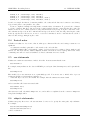
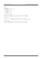
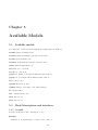
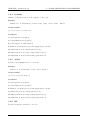
SUGAR 3.0: A MEMS Simulation Program (User’s Guide)
Document Authors - David Bindel, Jason Clark, Ningning Zhou
Revisions for Version 3.0 - David Garmire
Principal Investigators
Alice M. Agogino . . . . . . . . . . . . . . . . [email protected]
Zhaojun Bai . . . . . . . . . . . . . . . . . . . . . . . . . . . . [email protected]
James Demmel . . . . . . . . . . . . . . . . . . . [email protected]
Sanjay Govindjee . . . . . . . . . . . . . . . . . . [email protected]
Ming Gu . . . . . . . . . . . . . . . . . . . . . . . . . . . . [email protected]
Kristofer S. J. Pister . . . . . . . . . . . . . [email protected]
Graduated Students
Ningning Zhou . . . . . . . . . . . . . . . [email protected]
Graduate Students
David Bindel . . . . . . . . . . . . . . . . . . . . . . [email protected]
Jason V. Clark . . . . . . . . . . . . [email protected]
David Garmire . . . . . . . . . . . . . . . . . . . . . [email protected]
Raffi Kamalian . . . . . . . . . . . . . . . . . . . . . . [email protected]
Shyam Lakshmin . . . . . . . . . . . . . . . . . [email protected]
Jiawang Nie . . . . . . . . . . . . . . . . . . . . . . . . . [email protected]
Undergraduate Students
Wayne Kao . . . . . . . . . . . . . . . . . . . . . . . . . . . . . . . . . . [email protected]
Ernest Zhu . . . . . . . . . . . . . . . . . . . . . . . . . . . . . . . . . . . . . . . . . . . . . . . . . . .
20 April 2002
Contents
1 Introducing SUGAR
1.1 What is SUGAR? . . . . . . . . . .
1.2 A first example . . . . . . . . . . .
1.3 Installing SUGAR . . . . . . . . .
1.3.1 System requirements . . . .
1.3.2 Setting SUGAR paths . . .
1.3.3 Compiling external routines
1.4 Getting (and giving) help . . . . .
.
.
.
.
.
.
.
.
.
.
.
.
.
.
.
.
.
.
.
.
.
.
.
.
.
.
.
.
.
.
.
.
.
.
.
.
.
.
.
.
.
.
.
.
.
.
.
.
.
.
.
.
.
.
.
.
.
.
.
.
.
.
.
.
.
.
.
.
.
.
.
.
.
.
.
.
.
.
.
.
.
.
.
.
.
.
.
.
.
.
.
.
.
.
.
.
.
.
.
.
.
.
.
.
.
.
.
.
.
.
.
.
.
.
.
.
.
.
.
.
.
.
.
.
.
.
.
.
.
.
.
.
.
.
.
.
.
.
.
.
.
.
.
.
.
.
.
.
.
.
.
.
.
.
.
.
.
.
.
.
.
.
.
.
.
.
.
.
.
.
.
.
.
.
.
.
.
.
.
.
.
.
1
1
1
2
2
2
2
3
2 Describing Devices
2.1 Units and metric suffixes . . . . . . . . . . . . . . . .
2.2 Expressions . . . . . . . . . . . . . . . . . . . . . . .
2.3 Rotation angles . . . . . . . . . . . . . . . . . . . . .
2.4 Lexical notes . . . . . . . . . . . . . . . . . . . . . .
2.5 use statements . . . . . . . . . . . . . . . . . . . . .
2.6 addpath statements . . . . . . . . . . . . . . . . . .
2.7 node statements . . . . . . . . . . . . . . . . . . . .
2.8 element statements . . . . . . . . . . . . . . . . . .
2.9 Variables . . . . . . . . . . . . . . . . . . . . . . . .
2.10 material statements - Process parameter structures
2.11 subnet statements . . . . . . . . . . . . . . . . . . .
2.12 Arrays . . . . . . . . . . . . . . . . . . . . . . . . . .
2.13 Conditionals . . . . . . . . . . . . . . . . . . . . . . .
.
.
.
.
.
.
.
.
.
.
.
.
.
.
.
.
.
.
.
.
.
.
.
.
.
.
.
.
.
.
.
.
.
.
.
.
.
.
.
.
.
.
.
.
.
.
.
.
.
.
.
.
.
.
.
.
.
.
.
.
.
.
.
.
.
.
.
.
.
.
.
.
.
.
.
.
.
.
.
.
.
.
.
.
.
.
.
.
.
.
.
.
.
.
.
.
.
.
.
.
.
.
.
.
.
.
.
.
.
.
.
.
.
.
.
.
.
.
.
.
.
.
.
.
.
.
.
.
.
.
.
.
.
.
.
.
.
.
.
.
.
.
.
.
.
.
.
.
.
.
.
.
.
.
.
.
.
.
.
.
.
.
.
.
.
.
.
.
.
.
.
.
.
.
.
.
.
.
.
.
.
.
.
.
.
.
.
.
.
.
.
.
.
.
.
.
.
.
.
.
.
.
.
.
.
.
.
.
.
.
.
.
.
.
.
.
.
.
.
.
.
.
.
.
.
.
.
.
.
.
.
.
.
.
.
.
.
.
.
.
.
.
.
.
.
.
.
.
.
.
.
.
.
.
.
.
.
.
.
.
.
.
.
.
.
.
.
.
.
.
.
.
.
.
.
.
.
.
.
.
.
.
.
.
.
.
.
.
.
.
.
.
.
.
.
.
.
.
.
.
.
.
.
.
.
.
.
.
.
.
.
.
.
.
.
.
.
.
.
.
.
.
.
.
.
4
4
4
5
6
6
6
7
7
8
8
9
9
10
3 Analyzing Devices
3.1 Types of analysis . . . . . . . . .
3.2 Static analysis . . . . . . . . . .
3.3 Steady-state and Modal Analysis
3.4 Transient Analysis . . . . . . . .
.
.
.
.
.
.
.
.
.
.
.
.
.
.
.
.
.
.
.
.
.
.
.
.
.
.
.
.
.
.
.
.
.
.
.
.
.
.
.
.
.
.
.
.
.
.
.
.
.
.
.
.
.
.
.
.
.
.
.
.
.
.
.
.
.
.
.
.
.
.
.
.
.
.
.
.
.
.
.
.
.
.
.
.
.
.
.
.
.
.
.
.
.
.
.
.
.
.
.
.
.
.
.
.
.
.
.
.
.
.
.
.
.
.
.
.
.
.
.
.
.
.
.
.
.
.
.
.
.
.
.
.
.
.
.
.
.
.
.
.
.
.
.
.
.
.
.
.
.
.
.
.
.
.
.
.
.
.
.
.
.
.
.
.
.
.
.
.
.
.
.
.
.
.
.
.
.
.
.
.
.
.
.
12
12
12
13
14
4 Examples
4.1 Examples with explanations . . . . . . . . . .
4.1.1 cantilever example (demo dc1) . . . .
4.1.2 multiple beam example (demo dc2) . .
4.1.3 Beam gap structure (demo beamgap)
4.1.4 Modal analysis (demo mirror) . . . . .
4.1.5 Steady state analysis (demo ss) . . . .
4.1.6 Transient analysis (demo ta1gap) . . .
.
.
.
.
.
.
.
.
.
.
.
.
.
.
.
.
.
.
.
.
.
.
.
.
.
.
.
.
.
.
.
.
.
.
.
.
.
.
.
.
.
.
.
.
.
.
.
.
.
.
.
.
.
.
.
.
.
.
.
.
.
.
.
.
.
.
.
.
.
.
.
.
.
.
.
.
.
.
.
.
.
.
.
.
.
.
.
.
.
.
.
.
.
.
.
.
.
.
.
.
.
.
.
.
.
.
.
.
.
.
.
.
.
.
.
.
.
.
.
.
.
.
.
.
.
.
.
.
.
.
.
.
.
.
.
.
.
.
.
.
.
.
.
.
.
.
.
.
.
.
.
.
.
.
.
.
.
.
.
.
.
.
.
.
.
.
.
.
.
.
.
.
.
.
.
.
.
.
.
.
.
.
.
.
.
.
.
.
.
.
.
.
.
.
.
.
.
.
.
.
.
.
.
15
15
15
16
17
17
18
18
.
.
.
.
.
.
.
.
.
.
.
.
.
.
.
.
.
.
.
.
.
.
.
.
i
5 Available Models
5.1 Available models . . . . . . . . .
5.2 Model descriptions and interfaces
5.2.1 beam2d . . . . . . . . . .
5.2.2 beam2de . . . . . . . . . .
5.2.3 beam3d . . . . . . . . . .
5.2.4 beam3de . . . . . . . . . .
5.2.5 anchor . . . . . . . . . . .
5.2.6 f2d . . . . . . . . . . . . .
5.2.7 f3d . . . . . . . . . . . . .
5.2.8 gap2de . . . . . . . . . . .
5.2.9 gap3de . . . . . . . . . . .
5.2.10 Vsrc . . . . . . . . . . . .
5.2.11 eground . . . . . . . . . .
.
.
.
.
.
.
.
.
.
.
.
.
.
.
.
.
.
.
.
.
.
.
.
.
.
.
.
.
.
.
.
.
.
.
.
.
.
.
.
.
.
.
.
.
.
.
.
.
.
.
.
.
.
.
.
.
.
.
.
.
.
.
.
.
.
.
.
.
.
.
.
.
.
.
.
.
.
.
.
.
.
.
.
.
.
.
.
.
.
.
.
.
.
.
.
.
.
.
.
.
.
.
.
.
.
.
.
.
.
.
.
.
.
.
.
.
.
.
.
.
.
.
.
.
.
.
.
.
.
.
.
.
.
.
.
.
.
.
.
.
.
.
.
.
.
.
.
.
.
.
.
.
.
.
.
.
.
.
.
.
.
.
.
.
.
.
.
.
.
.
.
.
.
.
.
.
.
.
.
.
.
.
.
.
.
.
.
.
.
.
.
.
.
.
.
.
.
.
.
.
.
.
.
.
.
.
.
.
.
.
.
.
.
.
.
.
.
.
.
.
.
.
.
.
.
.
.
.
.
.
.
.
.
.
.
.
.
.
.
.
.
.
.
.
.
.
.
.
.
.
.
.
.
.
.
.
.
.
.
.
.
.
.
.
.
.
.
.
.
.
.
.
.
.
.
.
.
.
.
.
.
.
.
.
.
.
.
.
.
.
.
.
.
.
.
.
.
.
.
.
.
.
.
.
.
.
.
.
.
.
.
.
.
.
.
.
.
.
.
.
.
.
.
.
.
.
.
.
.
.
.
.
.
.
.
.
.
.
.
.
.
.
.
.
.
.
.
.
.
.
.
.
.
.
.
.
.
.
.
.
.
.
.
.
.
.
.
.
.
.
.
.
.
.
.
.
.
.
.
.
.
.
.
.
.
.
.
.
.
.
.
.
.
.
.
.
.
.
.
.
.
.
.
.
.
.
.
.
.
.
.
.
.
.
.
.
.
.
.
.
.
.
.
.
.
.
.
.
.
.
.
.
.
.
.
.
.
.
.
.
.
.
.
.
.
.
.
.
.
.
.
.
.
.
.
.
.
.
.
.
.
.
.
.
.
.
.
.
20
20
20
20
21
21
22
22
22
23
23
24
24
25
6 Function Reference
6.1 Load netlist . . . . . .
6.2 Device display . . . . .
6.3 Viewing displacements
6.4 Static analysis . . . .
6.5 Modal analysis . . . .
6.6 Steady state analysis .
6.7 Transient analysis . .
.
.
.
.
.
.
.
.
.
.
.
.
.
.
.
.
.
.
.
.
.
.
.
.
.
.
.
.
.
.
.
.
.
.
.
.
.
.
.
.
.
.
.
.
.
.
.
.
.
.
.
.
.
.
.
.
.
.
.
.
.
.
.
.
.
.
.
.
.
.
.
.
.
.
.
.
.
.
.
.
.
.
.
.
.
.
.
.
.
.
.
.
.
.
.
.
.
.
.
.
.
.
.
.
.
.
.
.
.
.
.
.
.
.
.
.
.
.
.
.
.
.
.
.
.
.
.
.
.
.
.
.
.
.
.
.
.
.
.
.
.
.
.
.
.
.
.
.
.
.
.
.
.
.
.
.
.
.
.
.
.
.
.
.
.
.
.
.
.
.
.
.
.
.
.
.
.
.
.
.
.
.
.
.
.
.
.
.
.
.
.
.
.
.
.
.
.
.
.
.
.
.
.
.
.
.
.
.
.
.
.
.
.
.
.
.
.
.
.
.
.
.
.
.
.
.
.
.
.
.
.
.
.
.
.
.
.
.
.
.
.
.
.
.
.
.
.
.
.
.
.
.
26
26
26
27
27
28
29
30
.
.
.
.
.
.
.
.
.
.
.
.
.
.
.
.
.
.
.
.
.
.
.
.
.
.
.
.
.
.
.
.
.
.
.
.
.
.
.
.
.
.
ii
Chapter 1
Introducing SUGAR
1.1
What is SUGAR?
In less than a decade, the MEMS community has leveraged nearly all the integrated-circuit community’s fabrication techniques, but little of the wealth of simulation capabilities. A wide range of student and professional
circuit designers regularly use circuit simulation tools like SPICE, while MEMS designers often resort to backof-the-envelope calculations. For three decades, development of IC CAD tools has gone hand-in-hand with the
development of IC processes. Tools for simulation will play a similar role in future advances in the design of
complicated micro-electromechanical systems.
SUGAR inherits its name and philosophy from SPICE. A MEMS designer can describe a device in a compact
netlist format, and very quickly simulate the device’s behavior. Using simple simulations in SUGAR, a designer
can quickly find problems in a design or try out new ideas. Later in the design process, a designer might run more
detailed simulations to check for subtle second-order effects; early in the design, a quick approximate solution is
key. SUGAR provides that quick solution.
The main components of SUGAR are a netlist interpreter (based on a derivative of the Lua language),
models written in MATLAB or C (possibly more languages in future revisions) describing the characteristics
of the different components, a command-line and gui which allows interaction and visualization of the specified
devices, and a SUGAR core that handles generated nodes and elements, mesh assembly, and analysis of devices.
1.2
A first example
Let’s first look at a simple example of how SUGAR is used. Perhaps we have just designed a simple test structure
in the MUMPS process, a long cantilever anchored at one end. We want to know how much it will deflect if we
apply a small force to the free end.
First, we need an input file, called a netlist, that describes the device. We save this netlist in the file
cantilever.net:
use("mumps.net")
use("stdlib.net")
A = node{0, 0, 0; name = "A"}
B = node{name = "B"}
anchor { A
; material=p1, l=10u, w=10u }
beam3d { A, B ; material=p1, l=100u, w=2u }
f3d
{ B
; F=50u, oz=90 }
The first line tells SUGAR that our device is made using the standard MUMPS process. The second and third
line define two nodes to be used later in describing the netlist’s elements. The fourth and fifth lines tell SUGAR
that the device is made of an anchor at node A, which is ten microns on a side; and a beam, two microns wide
1
CHAPTER 1: Introducing SUGAR
1.3. INSTALLING SUGAR
and one hundred long, which goes from the anchored end point A to the free end B. Both the anchor and the
beam are made of the poly1 layer, or p1. The sixth line describes a force of 50 micro-Newtons applied at a right
angle to the free end of the beam.
Using SUGAR, we only need to write three commands to see the effect of the force on the beam:
> net = cho_load(’cantilever.net’);
> q = cho_dc(net);
> cho_display(net, q);
The first command tells SUGAR to process the netlist description in cantilever.net. The result is a data
structure stored in the net variable that describes the device to other SUGAR routines. The cho dc function
does a static (DC) analysis of the device, and returns a vector representing the equilibrium position. Finally,
the third line causes SUGAR to display the displaced device.
1.3
Installing SUGAR
All the SUGAR software is available from the SUGAR home page at
http://bsac.berkeley.edu/cadtools/sugar
We update the software frequently; if you encounter problems, you may want to download the latest version
before devoting hours of your time (or ours!) to debugging.
There is also a web interface to SUGAR at:
http://sugar.millennium.berkeley.edu/
If you are building SUGAR for your particular system, note that you need to first make the noweb and Lua
tools in the sugar30/tools directory of the source tree. noweb (refer to http://www.eecs.harvard.edu/~nr/noweb/USA.html)
enables literate programming. The modified form of Lua (refer to http://www.lua.org/) is for the netlist and
command-line interpreter.
1.3.1
System requirements
To require SUGAR, you will need MATLAB release 5.2 or later. Version 6.0 is recommended. Because the
student edition of MATLAB 5 only handles matrices of a limited size, users of the student edition will only be
able to simulate small devices.
SUGAR is regularly tested using MATLAB 5.3 on Windows, Sun, HP, and Alpha systems, and is tested
using MATLAB 6.0 on Linux systems. We have not tested the software on other systems. If you would like to
use SUGAR on a different system, you will need to compile the external routines for that system, as described
later in this section.
1.3.2
Setting SUGAR paths
To use SUGAR, make sure that your MATLAB path is set correctly. In particular, make sure the analysis and
model subdirectories are included in your MATLAB path. This can be done from within MATLAB, e.g.
addpath /home/eecs/dbindel/sugar30/src/matlab
or from the Unix shell, by setting the MATLABPATH environment variable. In csh, for instance, this might be
setenv MATLABPATH /home/eecs/dbindel/sugar30/src/matlab
In the Windows version of MATLAB, you can also set the path from the “File” menu.
1.3.3
Compiling external routines
You will need to compile the external routines only if pre-compiled versions are not already available on your
system. To compile the routines, follow the directions in the included README file.
20 April 2002
2
CHAPTER 1: Introducing SUGAR
1.4
1.4. GETTING (AND GIVING) HELP
Getting (and giving) help
If you have concerns or difficulties using SUGAR which are not addressed in the manual sections, feel free to
post to
http://sourceforge.net/projects/mems
We will try to respond promptly.
SUGAR is research software; let us know if you would like to contribute models, analysis routines, or examples
to the SUGAR project.
20 April 2002
3
Chapter 2
Describing Devices
Devices in SUGAR are described by input files called netlists. In this chapter, we describe the features of the
netlist language which is a derivative of the Lua language.
2.1
Units and metric suffixes
By convention, the SUGAR model functions use the familiar MKS (meter-kilogram-second) system of units.
This means that beam lengths, for example, are measured in meters instead of micrometers. In order to make it
easier to type lengths of microns and pressures of gigapascals, we adopt a standard system of metric suffixes that
can be appended to SUGAR numbers. For example, a hundred micron length in SUGAR could be represented
as 100u as well as in scientific notation (100e-6) or as a simple decimal (0.0001). Similarly, a Young’s modulus
of 150 gigapascals might be written as 150G. Both suffixes and ordinary scientific notation can be used together,
too; 0.1e7u is a perfectly legitimate (if somewhat silly) way of writing the number 1.
The standard suffixes are:
d
c
m
u
n
p
f
a
2.2
deci
centi
milli
micro
nano
pico
femto
atto
10−1
10−2
10−3
10−6
10−9
10−12
10−15
10−18
h
k
M
G
T
P
E
hecto
kilo
mega
giga
tera
peta
exa
102
103
106
109
1012
1015
1018
Expressions
It’s often convenient to do simple calculations inside a netlist. For example, suppose I have defined a variable
beamL for the length of a beam in a device. Then we can define the length of another beam in terms of beamL:
use("mumps.net")
use("stdlib.net")
beamL = 100u
-- Make a beam one hundred microns long
-- make a beamL by beamL/2 rectangle
A = node{0, 0, 0; name = "A"}
B = node{name = "B"}
C = node{name = "C"}
D = node{name = "D"}
4
CHAPTER 2: Describing Devices
beam3d{
beam3d{
beam3d{
beam3d{
A,
C,
A,
B,
B
D
C
D
;
;
;
;
material=p1,
material=p1,
material=p1,
material=p1,
2.3. ROTATION ANGLES
w=2u,
w=2u,
w=2u,
w=2u,
l=beamL }
l=beamL }
l=beamL/2, oz=90 }
l=beamL/2, oz=90 }
SUGAR’s treatment of expressions are similar to Lisp’s treatment of expressions: we can add, subtract,
multiply, divide, exponentiate, and negate numbers, and also evaluate functions. All functionality described in
Lua is also available in SUGAR. All operations are left associative, so a + b + c is evaluated as (a + b) + c
rather than as a + (b + c). The order of operations, from highest precedence to lowest precedence, is
Level
7
6
5
4
3
2
1
Operators
| (logical or)
& (logical and)
== (equality), != (inequality), > (greater), < (less), >= (greater or equal), <= (less or equal)
- (add), + (subtract)
* (multiply), / (divide)
- (negate), ! (logical not)
^ (exponentiate)
As in C and MATLAB, there is no separate logical type. Non-zero numbers are interpreted as “true,” and
zero is interpreted as “false.” When a comparison or logical operation is true, it will evaluate to 1.
Besides numbers, SUGAR supports a string type. String literals are denoted by double quotes. Unlike C and
MATLAB, the backslash does not quote characters in SUGAR expressions: "\t" is a backslash followed by a t,
not a tab. Strings are values as well and can be used as operands to arithmetic or logical operations.
It is useful to note that a faster way of writing
if a then
x = a
elseif b then
x = b
else
x = c
end
is to form it as
x = a or b or c
Lua for SUGAR also contains the primitives addpath, node, material, element, and subnet, which will
be discussed more thoroughly later. addpath allows the inclusion of other directories for the use command.
node defines a node in 3 space for use later in defining elements. element invokes a model defined on a set
of nodal points with a set of parameters. subnet uses a function like declaration to parameterize netlists of
sub-components.
2.3
Rotation angles
In order to orient structures in SUGAR, users specify how each piece is rotated from a model coordinate frame
into its actual orientation in the structure. This specification can be done according to a global reference frame
by specifying the exact positions of the nodes (and allowing SUGAR to figure out the internal rotations) or by
specifying rotations of each component (may be done hierarchically in the case of subnets) and having SUGAR
position the nodes. Rotations are specified by a sequence of rotations about the x, z, and y axes, respectively.
The amount to rotate about each axis is given by angles ox, oz, and oy, given in degrees.
For many applications, most of the structure will lie initially in a single plane, and the only rotations used
to describe the device will be rotations about the z axis. For example, the lines
20 April 2002
5
CHAPTER 2: Describing Devices
beam3d{
beam3d{
beam3d{
beam3d{
A,
C,
A,
B,
B
D
C
D
;
;
;
;
material=p1,
material=p1,
material=p1,
material=p1,
2.4. LEXICAL NOTES
w=2u,
w=2u,
w=2u,
w=2u,
l=beamL }
l=beamL }
l=beamL/2, oz=90 }
l=beamL/2, oz=90 }
describe a rectangle; the first two beams run parallel to the x axis, and the latter two beams are rotated ninety
degrees in the plane to run parallel to the y axis.
For more complicated examples, it is important to remember that order matters. To go from local coordinates
to global coordinates, first the rotation about the x axis is applied, then the z axis, and then the y axis. For
instance, in the model coordinate system, a beam points in the direction (1, 0, 0), along the x axis. If we rotate
the beam first 90 degrees about the x axis and then 90 degrees about the z axis, it would point along the y axis,
in the (0, 1, 0) direction. If, however, we were to rotate the beam first about the z axis and then about the x
axis, it would end up pointing along the z axis.
2.4
Lexical notes
SUGAR 3.0 netlists are “free form”; that is, white space characters like tabs and carriage returns are not
significant.
A comment in a netlist begins with -- and extends to the end of the line.
A SUGAR identifier (like a C identifier) consists of a letter followed by a string of letters, numbers, and
underscores. The keywords use, subnet, addpath, element, and node are reserved (along with a slew of Lua
commands), and cannot be used as identifiers. See Lua documentation for more details.
2.5
use statements
Netlists can contain use statements to include other files. A use statement has the form
use("filename")
For example, many netlists use the data for MUMPS process layers defined in mumps.net, and begin with the
line
use("mumps.net")
Files included by a use statement are not particularly special. You can use use to include files of process
parameters, libraries of frequently-used subnets, etc.
A file will only be used once in a netlist. For example, if the file subnets.net started with
use("mumps.net")
and a test netlist called test.net started with
use("subnets.net")
use("mumps.net")
then test.net would only include mumps.net once, and would not complain about the contents of mumps.net
being defined multiple times.
2.6
addpath statements
Netlists can specify directories so the use statement does not need to specify the entire path, only a filename.
For example,
use("src/lua/base/mumps.net")
use("src/lua/base/std.net")
could be rewritten as
20 April 2002
6
CHAPTER 2: Describing Devices
2.7. NODE STATEMENTS
addpath("src/lua/base")
use("mumps.net")
use("std.net")
2.7
node statements
Nodes are connection points which have associated variables shared by attached elements. Mechanical nodes
also have positions.
An example of an absolute nodal declaration of node A at position (0, 0, 0) is
A = node{0, 0, 0; name = "A"}
An example of a relative nodal declaration of node B is
B = node{name = "B"}
When relative node positioning is used, SUGAR automatically ensures all of the node positions are generated
for each of the elements.
The syntax
node "A"
is used to refer to a node named “A” in the current scope. If no such node exists yet, then a new one is created.
For example, if we write
eground {node "ground"}
Vsrc
{node "ground", node "attach"; V=10}
the node “ground” is created in the first line, and the reference to node "ground" in the following line refers to
the same node.
2.8
element statements
The basic unit of a SUGAR netlist is an element line. For example,
crossbeam = element{ A, B; model="beam2d", material=p1, l=100u, w=2u }
is an element line describing a beam. This line consists of several fields:
• Before the equals sign, one may optionally put a name for that element; in this case, the element is named
crossbeam.
• Before the semicolon is a list of nodes. In this case, the specified beam connects nodes A and B. Elements
are connected together by sharing a common node. For instance, to attach a wider 100 micron beam to
the B end of the beam above, we might write
element { B, C; model="beam2d", material=p1, l=100u, w=5u }
Unlike in previous versions of SUGAR, node names in SUGAR 3.0 must begin with an alphabetic character.
• After the list of nodes comes a list of element parameters. Usually a process contains a model, a process,
and a list of parameters.
The name of the model for the element is specified as model="<model name>"; in this case, it is the twodimensional beam model beam2d. There are models for beams, anchors, electrical devices, etc.; a complete
list of models, along with information on how to build new models, can be found later in this document.
The process parameter structure for the element is specified as material=<process name>; in this case
the beam is fabricated in the first layer of polysilicon in a MUMPS process, named p1. By specifying the
20 April 2002
7
CHAPTER 2: Describing Devices
2.9. VARIABLES
process layer p1, a user informs the model function of common material parameters such as the Young’s
modulus for polysilicon and the thickness of the deposited layer. For models which require no process
information, such as models for external forces, the process field may be omitted.
In the example above, the model parameters consisted of the length and width of a beam; other models
will require other parameters. A parameter specification always has the form identifier = expression.
All permutations of arguments connected by commas are equivalent.
All the basic models in SUGAR have corresponding subnet wrappers. For example, these wrappers allow you
to rewrite
element { B, C; model="beam2d", material=p1, l=100u, w=5u }
as
beam2d{ B, C; material=p1, l=100u, w=5u }
The preferred way to invoke elements is with the latter syntax.
2.9
Variables
In order to allow users to experiment with variations on a simulation, or to do parameter sweeps, SUGAR allows
users to define variables in the Lua environment at load time. For example, a user might write
> params.nfingers = 10;
> net = cho_load(’comb.net’, params);
to create an instance of comb.net with comb drives having ten fingers. To test inside the netlist whether a
variable is defined, use the if statement
if not nfingers then
nfingers = 10 -- default is ten fingers
end
a shorter way to write the code above would be as
nfingers = nfingers or 10
SUGAR netlists may also include definitions, such as
long_length = 200u
short_length = 100u
avg_length = (long_length + short_length)/2
Netlist variables are scoped, so that a definition declared with the keyword, local, made inside a subnet (see
below) will not affect top-level element statements.
2.10
material statements - Process parameter structures
Physical parameters associated with a particular layer of a particular material are process parameters. An
example of the baseline process information for the polysilicon layers in MUMPS (default) is provided below
default = material {
Poisson = 0.3,
thermcond = 2.33,
viscosity = 1.78e-5,
fluid = 2e-6,
density = 2300,
Youngsmodulus = 165e9,
permittivity = 8.854e-12,
sheetresistance = 20
}
20 April 2002
--Poisson’s Ratio = 0.3
--Thermal conductivity Si = 2.33e-6/C
--Viscosity (of air) = 1.78e-5
--Between the device and the substrate.
--Material density = 2300 kg/m^3
--Young’s modulus = 1.65e11 N/m^2
--permittivity: C^2/(uN.um^2)=(C.s)^2/kg.um^3
--Poly-Si sheet resistance [ohm/square]
8
CHAPTER 2: Describing Devices
2.11. SUBNET STATEMENTS
In general a process definition has the form name = material {...}, where material is a keyword, name is
the name to be given to the process information.
Process parameter structures may be derived from other process parameter structures. For example, a 2
micron poly layer named p1 might be written
p1 = material {
parent = default,
h = 2u
}
This layer automatically includes all the definitions made in the default process parameter structure.
2.11
subnet statements
Subnets provide users with a means to extend the set of available models without leaving SUGAR. An example
subnet for a single unit of a serpentine structure is shown below:
subnet serpent( A, F, material, unitwid, unitlen, beamw )
beamw = beamw or 2u;
len2 = unitlen/2
beam2d{ A, node "b";
material=material, l=unitwid/2,
beam2d{ node "b", node "c"; material=material, l=len2,
beam2d{ node "c", node "d"; material=material, l=unitwid,
beam2d{ node "d", node "e"; material=material, l=len2,
beam2d{ node "e", F;
material=material, l=unitwid/2,
end
w=beamw, oz=-90 }
w=beamw }
w=beamw, oz=90 }
w=beamw }
w=beamw, oz=-90 }
Element lines using subnets are invoked in the same manner as element lines using model functions built in
MATLAB
serp1 = serpent {X, Y; material=p1, unitwid=10u, unitlen=10u}
serpent {y, z ; material=p1, unitwid=10u, unitlen=10u, w=3u}
The parent process for a subnet is the process specified in creating an instance of that subnet. In the above
example, the p1 process information would be used for the beams in the serpent subnet.
In general, a subnet definition consists of the keyword subnet, a name for the subnet model, a set of arguments,
and a code block followed by end. The code block may include definitions, element lines, and array structures
(see below).
Sometimes it may be necessary to access variables attached to nodes internal to a netlist. For example, in
the above example we might be interested in the version of node b for subnet instance serp1. In the analysis
functions, that node would be referred to as serp1.b. It would not be valid to refer to node x as serp1.A, since
x already has a name defined outside the subnet.
Subnet instances that are not explicitly named, like the second serpent element in the example above, are
assigned names consisting of anon followed by some number. It is possible to use a name like anon1.b to refer
to the b node in the second line, but it is not recommended since the internal naming schemes for anonymous
elements are subject to future change.
2.12
Arrays
SUGAR supports arrays of structures through the same syntax as Lua. Arrays are built enclosed in braces and
referenced using brackets. For example, the following code fragment creates a spring composed of twenty of the
serpentine units from the subnet example and anchors it at one end:
link = { node {} };
anchor {p[1]; material=p1, l=5u, w=5u}
20 April 2002
9
CHAPTER 2: Describing Devices
2.13. CONDITIONALS
for k = 1,nlinks do
link[k+1] = node {};
serpent {link[k], link[k+1]; material=p1, unitwid=10u, unitlen=10u, w=2u}
end
Note that link needs to first be initialized. It is possible to have names with multiple indices as well (eg
link[i][j])). The index variable is only valid within the loop body.
The general syntax of a for loop is
for index = lowerbound, upperbound [, increment] do
... code lines ...
end
where index is the name of the index variable, lowerbound is an expression for the lower bound of the loop, and
upperbound is an espression for the upper bound of a loop.
2.13
Conditionals
SUGAR supports if statements of the form
if expression then
... code lines ...
end
and
if expression then
... code lines ...
else
... code lines ...
end
The main purpose of if statements is to give some flexibility to subnet writers. For example, suppose I
wanted a beam that would automatically compute its electrical resistance if one was not provided. I could do
that with the following subnet:
subnet mybeam( A, B, l, w, h, R, resistivity )
-- If R is nil, then the user didn’t specify anything to override
-- the default, so we’ll help calculate the resistance.
if not R then
resistance = resistivity * l/(w*h)
beam3de {A, B; material=parent, l=l, w=w, h=h, R=resistance}
-- Otherwise, we’ll just accept whatever the user wrote in
else
beam3de {A, B; material=parent, l=l, w=w, h=h, R=R}
end
end
There are a few caveats that go with this example:
1. Usually, resistivity would be defined in the process information when an instance of mybeam was created.
2. A briefer way to write this example would be
subnet mybeam(A, B, l, w, h, R, resistivity)
beam3de{A, B; material=parent, l=l, w=w, h=h,
R=( R or (resistivity * l/(w*h)) )}
end
20 April 2002
10
CHAPTER 2: Describing Devices
2.13. CONDITIONALS
The local statement restricts the variable to the given scope.
3. The SUGAR netlist language is designed to be extensible, yet it is limited. By using the if statement,
it is possible to write arbitrarily complicated netlists, with constructs like recursive subnets or even more
subtle beasts. Exercise good taste when you write netlists, and try to relegate any subtle and complicated
coding tasks to MATLAB instead of to the SUGAR netlist language.
20 April 2002
11
Chapter 3
Analyzing Devices
3.1
Types of analysis
SUGAR supports three basic styles of analysis:
Static analysis : In static analysis, we find the equilibrium state of a device. Static analysis is sometimes
called DC analysis by analogy to the equilibrium analysis for direct current circuits.
Linearized analysis : A linearized approximation to a system near equilibrium can provide valuable information about the stability of the system and the nature of small oscillations about equilibrium. SUGAR
provides two flavors of linearized analysis:
• In modal analysis, the characteristic modes of the system (and their corresponding frequencies) are
determined. SUGAR can display the shapes of the displacements corresponding to various modes.
• In steady-state analysis, SUGAR computes the frequency response of a user-specified variable when
another user-specified variable is sinusoidally excited. The output of steady state analysis is Bode
plots.
Transient analysis : In transient analysis (or dynamic analysis), the motion of the system is integrated forward
in time. Transient analysis in SUGAR is still somewhat unreliable; we hope to have better support for it
soon.
3.2
Static analysis
In static analysis, we attempt to find an equilibrium state for a MEMS device. In the most general case, the
equilibrium may not be unique; in this case, SUGAR will usually find the equilibrium position closest to where
it starts looking (which, by default, is the undisplaced position).
The equilibrium state is characterized by a collection of force and moment balance equations (and their
electrical and thermal analogues):
F (x) = 0
where x is a vector of displacements from the original positions (and voltages, temperatures, etc) of the device.
We solve these equations using a standard Newton-Raphson iteration. For linear problems, a Newton-Raphson
iteration will converge in one steps; for nonlinear problems, the iteration may never converge. Currently, SUGAR
assumes the iteration has converged when the size of the change between iterations is sufficently small in an
appropriately scaled norm. If convergence has not set in after 40 iterations, the routine exits with a diagnostic
message.
The function to perform static analysis is cho dc:
res = cho_dc(net, q0, is_sp)
12
CHAPTER 3: Analyzing Devices
3.3. STEADY-STATE AND MODAL ANALYSIS
The first argument, net, is the netlist structure returned from cho load. The other arguments are optional.
The starting value for the iteration is given by q0; by default, the iteration starts at the undisplaced position
(q0 = 0). The flag is sp tells the routine whether it should use sparse solvers or not; by default, the flag is
true (sparse solvers are used). The function returns a vector of displacements to reach the computed equilibrium
(res.q), and a flag that indicates whether the iteration converged (res.converged).
In some cases, it is possible to find tricky equilibrium positions by approaching them step-by-step. For
example, suppose we wanted to determine the equilibrium position of a device near a pull-in voltage. As we
approach the critical voltage, it becomes more difficult to find the equilibrium position, and past the critical
voltage, no equilibrium exists. If the commands
params.V = Vfinal;
net = cho_load(’device.net’, params);
q = cho_dc(net)
fail, we could try
q = [];
for V = 0:.5:Vfinal
params.V = V
net = cho_load(’device.net’, params);
q = cho_dc(net, q);
end
Even if we were still unable to find the equilibrium position, we might get useful information from seeing how
nearly we were able to approach the final voltage, and what the equilibrium was at the last point where we were
able to find it.
There are two ways to view the results of a static analysis:
1. We can view individual components of the displacement vector using the command cho dq view:
% Find displacement of the y coordinate at node ’tip’
tipy = cho_dq_view(q, net, ’tip’, ’y’);
Alternately, we could look up the index of the tip y coordinate, and then look at the corresponding entry
of the q vector:
% Find displacement of the y coordinate at node ’tip’
tipy_index = lookup_coord(net, ’tip’, ’y’);
tipy = q(tipy_index);
2. We can display the shape of the displaced structure using the cho display routine:
% Display the undisplaced structure in figure 1,
% and the displaced structure in figure 2.
q = cho_dc(net);
figure(1); cho_display(net);
figure(2); cho_display(net, q);
3.3
Steady-state and Modal Analysis
We determine system behavior near equilibrium by analyzing the linearized system. In modal analysis, we find
the resonant behavior of the structure, assuming no damping, by solving the eigenproblem
det(λ2 M − K) = 0
The eigenvalues give the resonant frequencies, and the corresponding eigenvectors give the resonant modes. The
routine cho_mode returns selected frequencies and mode shapes for a structure, along with the operating point
20 April 2002
13
CHAPTER 3: Analyzing Devices
3.4. TRANSIENT ANALYSIS
at which linearization took place. Mode shapes can be viewed graphically using the cho_modeshape commands.
For small problems, the default dense solvers are adequate; for larger problems, users should select the number
of modes they want, and those modes will be computed using a less expensive iterative method.
To use the steady-state analysis routine, a user specifies a single input degree of freedom and a single output
degree of freedom, usually by naming a nodal variable. SUGAR then draws a Bode plot illustrating the amplitude
gain and phase shift between a harmonic excitation at the input and a measured harmonic at the output. Note
that, unlike the modal analysis routine, the steady state routine does not discard damping terms.
3.4
Transient Analysis
Note: Note yet in SUGAR 3.0
20 April 2002
14
Chapter 4
Examples
This section describes how to use SUGAR 3.0 by examples. The netlists, commands for running analysis, and
output are shown. For convenience, all netlist files given here are available in the SUGAR demo directory
(converted from 2.0). Netlist format is defined in chapter 2.
4.1
4.1.1
Examples with explanations
cantilever example (demo dc1)
This demo shows how to simulate the deflection of a beam due to an external force, where the beam is fixed at
one end. It shows to make the netlist, how run static analysis, and obtain graphical output.
To model the beam a 3D linear beam model called beam3d will be used. If a planar beam is desired, simply
replace the model b3dm with beam2d in line 2 of following netlist.
Netlist
The following netlist is created by opening a text editor, entering the 3 lines of netlist text shown below, and
saved as cantilever.net. The 3 text lines represent an anchor, beam, and force.
-- ‘cantilever.net’
use("mumps.net")
use("stdlib.net")
anchor {node "substrate"; material=p1, l=10u, w=10u, h=10u}
beam3d {node "substrate", node "tip"; material=p1, l=100u, w=2u, h=2u}
f3d
{node "tip"; F=2u, oz=90}
The first line in the netlist includes a process file “mumps.net”. All process information such as layer thickness,
Young’s modulus etc. are defined in “mumps.net”. The second line includes the standard library file “stdlib.net”.
The first line in the netlist represents the anchor element. Anchors are the MEMS components that mechanically ground flexible structures to the substrate. Without anchors, structures would be statically indeterminate.
The material properties of the anchor are given in process file ”mumps.net”. The fabrication layer of this
process is p1.
The anchor is attached to the substrate by the node labeled substrate. Notice that both the anchor element
and beam element (described below) contain the node labeled substrate. The anchor is coupled to the beam
through node substrate.
The parameters section of this line of text provides the geometry and orientation, where the length, width
are 10 microns.
The second element is a flexible beam. The model used for this beam is called beam3d, which is described
in appendix. The fabrication layer with which this beam is composed of is the p1 layer (i.e. the first layer of
15
CHAPTER 4: Examples
4.1. EXAMPLES WITH EXPLANATIONS
polysilicon). It is fixed on one end due to its connection to the anchor through the node labeled substrate. The
opposite end of the beam, labeled tip, is free to move.
The last section of this line provides geometry and orientation. The beam extends to the right, from node
substrate to node tip.
The final line is a force applied at the free end of the beam (node tip). The magnitude of the force is given
as 2 microNewtons. The orientation of the force vector is in the y- direction since it was rotated from its default
position along the positive x-axis.
Command
Once the netlist text file is created, load it into Matlab with the cho load command. Then static analysis may
be performed, which finds a final equilibrium state of the system. Running static analysis on the above netlist
requires 3 commands. Within the Matlab workspace:
1. load the netlist,
2. perform static analysis on it, and
3. display the results:
net = cho_load(’cantilever.net’);
dq = cho_dc(net);
cho_display(net,dq);
The first command loads the text file called cantilever.net into a variable called net. The net variable contains
all of the important information in the netlist file.
The second line performs the static analysis. The cho dc command takes net as its input. Using the parameter
values given in the netlist and the parameterized element models described in appendix, it calculates the deflection
of the structure. The displacement vector dq is the output of cho dc.
Incidentally, cho stands for the basic building locks of sugar (i.e. carbon, hydrogen, oxygen).
Using geometries and orientations from net and node displacements from dq as input to cho display, SUGAR
can graphically display the deflected structure in Matlab.
To display original, non-deflected structure, simply type
cho_display(net);
After the structure is displayed, left clicking and dragging within the display window may adjust the view. The
magnification buttons in the display window may be used to zoom in and out by first clicking on, say the zoom-in
(+), followed by pointing and clicking on the display window at the precise position that is to be magnified.
4.1.2
multiple beam example (demo dc2)
This demo is similar to above demo with the exception that it uses multiple beams and it is deflected by a
moment. Netlist is as following:
Netlist
-- ’multibeam.net’
use("mumps.net")
use("stdlib.net")
anchor
beam3d
beam3d
beam3d
beam3d
f3d
{node
{node
{node
{node
{node
{node
20 April 2002
"substrate"; material=p1, l=10u, w=10u, oz=180}
"substrate", node "A"; material=p1, l=100u, w=10u}
"A", node "B"; material=p1, l=50u, w=4u, oz=45}
"A", node "C"; material=p1, l=50u, w=4u, oz=-45}
"C", node "D"; material=p1, l=50u, w=4u, oy=-45}
"D"; M=1n}
16
CHAPTER 4: Examples
4.1. EXAMPLES WITH EXPLANATIONS
As before, each element is connected at shared nodes. The commands to load the netlist, do the analysis,
and display the non-deflected and deflected figures are
net = cho_load(’multibeam.net’);
dq = cho_dc(net);
figure(1); cho_display(net);
figure(2); cho_display(net,dq);
4.1.3
Beam gap structure (demo beamgap)
This is a 2D coupled electrical and mechanical domain analysis. It contains electrical voltage source, electrical
ground, electro-mechanical anchors, beam and gap. The netlist and structure of this demo are as following:
Netlist
-- ‘beamgap2e.net’
use "mumps.net"
use "stdlib.net"
Vsrc
eground
anchor
beam2de
{node "A", node "f"; V = 10}
{node "f"}
{node "A", p1; l=5u, w=10u, oz=180}
{node "A", node "b", p1;
l=100u, w=2u, h=2u, R=100}
gap2de {node "b", node "c", node "D", node "E", p1;
l=100u, w1=10u, w2=5u, gap=2u, R1=100, R2=100}
eground {node "D"}
eground {node "E"}
anchor {node "D", p1; l=5u, w=10u, oz=-90}
anchor {node "E", p1; l=5u, w=10u, oz=-90}
Equilibrium displacements have been calculated at an input voltage 10v. The deflected structure is shown as
following:
4.1.4
Modal analysis (demo mirror)
This is a 3D mechanical modal analysis for a mirror structure. 3D mechanical anchors and beams are included.
Resonant frequencies have been calculated and the first to fourth mode shapes are displayed. Below are the
netlist and demo pictures
Netlist
-- ‘mirror.net’
use "mumps.net"
use "stdlib.net"
anchor
beam3d
beam3d
anchor
{node
{node
{node
{node
"b";
material=p1,
"b", node "c"; material=p1,
"d", node "e"; material=p1,
"e";
material=p1,
l=10u,
l=80u,
l=80u,
l=10u,
w=10u,
w=2u,
w=2u,
w=10u,
oz= 90,
oz=-90,
oz=-90,
oz=-90,
h=8u}
h=2u}
h=2u}
h=8u}
-- outer frame:
beam3d {node "c", node "f"; material=p1, l=100u, w=20u, oz=-90, h=4u}
beam3d {node "f", node "d"; material=p1, l=100u, w=20u, oz=-90, h=4u}
beam3d {node "c1", node "f1"; material=p1, l=100u, w=20u, oz=-90, h=4u}
20 April 2002
17
CHAPTER 4: Examples
4.1. EXAMPLES WITH EXPLANATIONS
beam3d {node "f1", node "d1"; material=p1, l=100u, w=20u, oz=-90, h=4u}
beam3d {node "c", node "c1"; material=p1, l=200u, w=20u, oz= 0, h=4u}
beam3d {node "d", node "d1"; material=p1, l=200u, w=20u, oz= 0, h=4u}
-- inner torsion hinges:
beam3d {node "g3", node "f1"; material=p1, l=40u,
beam3d {node "f", node "g6"; material=p1, l=40u,
oz=0,
oz=0,
h=2u}
h=2u}
-- inner solid "plate":
beam3d {node "g6", node "g3"; material=p1, l=120u, w=140u, oz=0,
h=4u}
-- rear lever:
beam3d {node "h",
h=4u}
4.1.5
node "f";
material=p1, l=75u,
w=2u,
w=2u,
w=80u,
oz=0,
Steady state analysis (demo ss)
This is a 2D steady state analysis for a resonator as following:
Netlist
-- ’multmode_m.net’
use("mumps.net")
use("stdlib.net")
anchor
beam2d
anchor
beam2d
beam2d
beam2d
beam2d
beam2d
beam2d
beam2d
beam2d
beam2d
beam2d
beam2d
beam2d
beam2d
beam2d
4.1.6
{node
{node
{node
{node
{node
{node
{node
{node
{node
{node
{node
{node
{node
{node
{node
{node
{node
"A";
"A",
"B";
"B",
"D",
"D",
"E",
"F",
"G",
"H",
"I",
"I",
"J",
"L",
"K",
"J",
"M",
material=p1,
node "D"; material=p1,
material=p1,
node "E"; material=p1,
node "F"; material=p1,
node "E"; material=p1,
node "G"; material=p1,
node "H"; material=p1,
node "L"; material=p1,
node "I"; material=p1,
node "O"; material=p1,
node "J"; material=p1,
node "K"; material=p1,
node "K"; material=p1,
node "P"; material=p1,
node "M"; material=p1,
node "N"; material=p1,
l=5u,
l=150u,
l=5u,
l=150u,
l=50u,
l=50u,
l=50u,
l=50u,
l=150u,
l=50u,
l=50u,
l=75u,
l=75u,
l=50u,
l=50u,
l=300u,
l=196u,
oz=0,
oz=180,
oz=0,
oz=180,
oz=90,
oz=-90,
oz=-90,
oz=0,
oz=0,
oz=0,
oz=0,
oz=-90,
oz=-90,
oz=0,
oz=0,
oz=0,
oz=0,
w=10u
w=2u
w=10u
w=2u
w=5u
w=5u
w=5u
w=2u
w=2u
w=20u
w=20u
w=20u
w=20u
w=20u
w=20u
w=2u
w=116u
}
}
}
}
}
}
}
}
}
}
}
}
}
}
}
}
}
Transient analysis (demo ta1gap)
Note: This demo has not yet been converted to SUGAR 3.0
This is a 3D electromechanical transient analysis for a gap-closing actuator. A piecewise linear voltage V(t)
is applied across the page. The voltage V(t) ramps from 5V at t=10usec to 12V at t=500usec, and then drops to
0V. The displacement component of node C in the direction of force is observed below. The initial voltage step
causes the device to oscillate. At the voltage increases at a linear rate, the gap decreases at a nonlinear rate due
to the electrostatic force increasing proportionally to 1/gap(q)2 . This force also causes the period of oscillation
to increase. Once the voltage is removed, the actuator exponentially decays back to equilibrium due to viscous
Couette air damping between the beams and the substrate.
20 April 2002
18
CHAPTER 4: Examples
4.1. EXAMPLES WITH EXPLANATIONS
Netlist
use("mumps.net")
a = node{0, 0, 0; name = "a"}
b = node{name = "b"}
c = node{name = "c"}
d = node{name = "d"}
e = node{name = "e"}
-- beam and it’s anchor:
anchor {a; material=p1, l=5u, w=10u, oz=180, ox=0, oy=0, h=10u}
beam2de {a, b; material=p1, l=100u, w=4u, oz=0, ox=0, oy=0, h=4u}
-- electrostatic
gapV2 {b, c, d, e; material=p1, V1=5, t1=10u, V2=12, t2=500u,
l=100u, w1=4u, w2=4u, oz=0, ox=0, oy=0, h=4u, gap=2u}
-- gap anchors
anchor {d; material=p1, l=5u, w=10u, oz=-90, ox=0, oy=0, h=10u}
anchor {e; material=p1, l=5u, w=10u, oz=-90, ox=0, oy=0, h=10u}
20 April 2002
19
Chapter 5
Available Models
5.1
Available models
Note that some of these models are implemented using subnets in stdlib.net.
beam2d planar mechanical beam
beam2de planar mechanical beam and electric resistor
beam3d 3D mechanical beam
beam3de 3D mechanical beam and electronic resistor
anchor 0D mechanical fixed node
f2d planar force or moment
f3d 3D force or moment
gap2de two planar electrostatic mechanical beams, resistors
gap3de two electrostatic 3D mechanical beams, resistors
Vsrc Voltage source
eground Electronic ground
comb2d N-finger electrostatic comb, 2D mechanical
R constant resistor
Isrc constant current source
nmos nmos model
pmos pmos model
5.2
5.2.1
Model descriptions and interfaces
beam2d
Describes an in-plane beam connecting two nodes.
Example:
beam2d { A, B; material=p1, l=100u, w=5u, oz=10 }
20
CHAPTER 5: Available Models
5.2. MODEL DESCRIPTIONS AND INTERFACES
Nodal variables:
{x, y, rz} at both nodes
Parameters
l beam length in meters (required)
w beam width in meters (required)
h thickness of beam in meters (optional; supplied in process info)
oz initial rotation about beam’s z-axis (required if not 0)
5.2.2
beam2de
Similar to beam2d but adds electronic resistance to the beam.
Example
beam2de { A, B; material=p1, l=100u, w=5u, oz=10, R=100 }
Nodal variables
{x, y, rz, e} at both nodes
Parameters
l beam length meters (required)
w beam width in meters (required)
R beam resistance in ohms (required)
h thickness of beam in meters (optional; supplied in process info)
oz initial rotation about beam’s z -axis (required if not 0)
5.2.3
beam3d
Similar to beam2d but can be rotated out-of-plane.
Example
beam3d { A, B; material=p1, l=100u, w=5u, oy=20, oz=10, ox=45 }
Nodal variables
{x, y, z, rx, ry, rz} at both nodes
Parameters
l beam length meters (required)
w beam width in meters (required)
h thickness of beam in meters (optional; supplied in process info)
oy initial rotation about y-axis (required if not 0)
oz initial rotation about beam’s z -axis (required if not 0)
ox initial twist about the beam’s x-axis (required if not 0)
20 April 2002
21
CHAPTER 5: Available Models
5.2.4
5.2. MODEL DESCRIPTIONS AND INTERFACES
beam3de
Similar to beam3d but adds electronic resistance to the beam.
Example
beam3de { A, B; material=p1, l=100u, w=5u, oy=20, oz=10, ox=45,
R=100}
Nodal variables
{x, y, z, rx, ry, rz, e} at both nodes
Parameters
l beam length meters (required)
w beam width in meters (required)
R beam resistance in ohms (required)
h thickness of beam in meters (optional; supplied in process info)
oy initial rotation about y-axis (required if not 0)
oz initial rotation about beam’s z -axis (required if not 0)
ox initial twist about the beam’s x-axis (required if not 0)
5.2.5
anchor
Describes a mechanically fixed node. 3D or 2D.
Example
anchor { A, B; material=p1, l=10u, w=10u, h=10u }
Nodal variables
{x, y, z, rx, ry, rz} at both nodes
Parameters
l beam length meters (required)
w beam width in meters (required)
h thickness of beam in meters (optional; supplied in process info)
oy initial rotation about y-axis (required if not 0)
oz initial rotation about beam’s z -axis (required if not 0)
ox initial twist about the beam’s x-axis (required if not 0)
5.2.6
f2d
Describes an in-plane external force at a node.
20 April 2002
22
CHAPTER 5: Available Models
5.2. MODEL DESCRIPTIONS AND INTERFACES
Example
f2d { A; F=10u, oz=45 }
f2d { A; M=1u, oz=45 }
Nodal variables
{x, y, rz} at node
Parameters
F force in Newtons (required if M is not used)
M moment in Newton-meters (required is F is not used)
oy initial rotation about y-axis (required if not 0)
oz initial rotation about the vetors’s z -axis (required if not 0)
5.2.7
f3d
Describes a 3D external force at a node.
Example
f3d { A; F=10u, oy=35, oz=45 }
f3d { A; M=1u, oy=35, oz=45 }
Nodal variables
{x, y, z, rx, ry, rz} at node
Parameters
F force in Newtons (required if M is not used)
M moment in Newton-meters (required is F is not used)
oy initial rotation about y-axis (required if not 0)
oz initial rotation about the vectors’s z -axis (required if not 0)
5.2.8
gap2de
Describes a 2D electrostatic gap, which consists of two electronic, mechanical beams.
Example
gap2de { a, b, c, d; material=p1, l=100u, w1=5u, w2=5u,
oz=0, gap=2u, R1=100, R2=100 }
Nodal variables
{x, y, z, rx, ry, rz, e} at all four nodes
20 April 2002
23
CHAPTER 5: Available Models
5.2. MODEL DESCRIPTIONS AND INTERFACES
Parameters
l beam length meters (required)
w1 beam1 width in meters (required)
w1 beam2 width in meters (required)
gap initial gap spacing
h thickness of both beams in meters (optional; supplied in process info)
R1 beam1 resistance in ohms (required)
R2 beam2 resistance in ohms (required)
oz initial rotation about beam1’s z -axis (required if not 0)
5.2.9
gap3de
Describes a 2D electrostatic gap, which consists of two electronic, mechanical beams.
Example
gap3de { a, b, c, d; material=p1, l=100u, w1=5u, w2=5u,
oz=0, gap=2u, R1=100, R2=100 }
Nodal variables
{x, y, z, rx, ry, rz, e} at all four nodes
Parameters
l beam length meters (required)
w1 beam1 width in meters (required)
w1 beam2 width in meters (required)
gap initial gap spacing
h thickness of both beams in meters (optional; supplied in process info)
R1 beam1 resistance in ohms (required)
R2 beam2 resistance in ohms (required)
oy initial rotation about y-axis (required if not 0)
oz initial rotation about beam1’s z -axis (required if not 0)
ox initial twist about the beam1’s x-axis (required if not 0)
5.2.10
Vsrc
Describes a voltage source.
Example
Vsrc { e, d; V=5 }
See Fig 5 for nodes. Note: only mechanical element display.
20 April 2002
24
CHAPTER 5: Available Models
5.2. MODEL DESCRIPTIONS AND INTERFACES
Nodal variables
{e} at both nodes
Parameters
V voltage in volts (required)
5.2.11
eground
Describes a electronic ground.
Example
eground { e }
Note: only mechanical elements display.
Nodal variables
{e} at nodes
Parameters
none
20 April 2002
25
Chapter 6
Function Reference
6.1
Load netlist
Calling sequence
net = cho_load(name, params)
Loads and processes a netlist.
Inputs
name String naming the netlist file to be loaded
params (Optional) - a structure whose entries are the values of the parameters to be overridden.
Example
nfingers = 10;
net = cho_load(’comb.net’, params);
6.2
% Set the nfingers parameter
% Load netlist
Device display
Calling sequence
cho_display(net, q)
Display the mechanical structure described by a netlist.
Inputs
net Netlist structure returned from calling cho load
q (Optional) - the displacement of the original structure, as returned by the static analysis routine or the
transient analysis routine. If q is unspecified, the undisplaced structure will be displayed.
Example
net = cho_load(’beamgap.net’);
cho_display(net);
% Load netlist for beam-gap system
% Display undisplaced structure
26
CHAPTER 6: Function Reference
6.3. VIEWING DISPLACEMENTS
Caveats
There is no display of electrical components.
6.3
Viewing displacements
Calling sequence
dqcoord = cho_dq_coord(dq, net, node, coord);
Extract the displacement corresponding to a particular coordinate from a displacement vector q (as output
by cho dc), or an array of displacement vectors (as output by cho ta).
Note that a node “node” completely internal to an instance “foo” of some subnet would be named “node.foo”.
Inputs
dq : Displacement vector or array of displacement vectors.
net : Netlist structure returned from calling cho load
node : Name of node.
coord : Name of coordinate at indicated node.
Outputs
dqcoord : Value (or vector of values) from dq associated with the indicated coordinate.
Example
net = cho_load(’beamgap.net’);
dq = cho_dc(net);
dy = cho_dq_view(dq, net, ’c’, ’y’);
6.4
% Load netlist
% Perform static analysis
% Get the y component at c
Static analysis
Calling sequence
q = cho_dc(net, q0, is_sp);
Finds a solution of the equilibrium equations
Kx = F (x)
using a Newton-Raphson method.
Inputs
net : Netlist structure returned from calling cho load
q0 : (Optional) Starting guess at the displacements from starting position for an equilibrium position. If no q0
is provided, or if q0 = the search will start at q0 of 0.
is sp : (Optional) If true, the code will use sparse solvers. The current default is true (use sparse solvers).
Outputs
q : The computed equilibrium state, expressed as displacements from the initial position.
20 April 2002
27
CHAPTER 6: Function Reference
6.5. MODAL ANALYSIS
Example
net = cho_load(’beamgap.net’);
dq = cho_dc(net);
cho_display(net, dq);
% Load netlist for beam-gap system
% Perform static analysis
% Display the deflected structure
Caveats
The zero-finder currently used by SUGAR is very simple, and may fail to converge for some problems. If the
function fails to converge after 40 iterations, it will exit and print a warning diagnostic:
Warning: DC solution finder did not converge after 40 iterations
In this case, the result q returned by the routine is likely to be useless. Failure to find equilibrium occurs in such
cases as an electrostatically actuated gap operating near pull-in voltage.
When SUGAR finds an equilibrium point, it may not always be the equilibrium point desired. In the case of
an electrostatically actuated gap, for example, there are two equilibria below pull-in voltage: one stable and one
unstable. When the equilibria are close together, especially with respect to the distance from the starting point
q0, the solver may move to an unstable equilibrium.
Good initial guesses for an equilibrium point can often be attained by finding the equilibrium point for a
“nearby” problem. For example, in trying to find the equilibrium point for a electrostatically actuated gap
operating near pull-in, a good initial guess q0 would be the output of a static analysis for the same device at a
lower voltage.
6.5
Modal analysis
Analysis routine
Calling sequence
[freq, egv, q0] = cho_mode(net, nmodes, q0, find_dc)
Find the resonating frequencies and corresponding mode shapes (eigenvalues and eigenvectors) for the linearized system about an equilibrium point.
Inputs
net : Netlist structure returned from calling cho load.
nmodes : (Optional) If nmodes > 0, use sparse solvers to get nmodes modes If nmodes == 0, use the usual dense
solver to get all the modes If nmodes < 0, solve with eig(K \ M) rather than eig(M,K). This last option
can potentially cause trouble (for instance, if K is singular), but it is faster.
q0 : (Optional) Equilibrium operating point, or initial guess for a search for an equilibrium operating point. If
not supplied, of if q0 = , the routine will search for an equilibrium point near 0.
find dc : (Optional) If true, search for an equilibrium point near the supplied q0.
Outputs
freq : Vector of resonating frequencies (eigenvalues)
egv : Array of corresponding mode shapes (eigenvectors)
q0 : Equilibrium point about which the system was linearized
20 April 2002
28
CHAPTER 6: Function Reference
6.6. STEADY STATE ANALYSIS
Display routine
Calling sequence
cho_modeshape(net, freq, egv, q0, s, num)
Display the shape of a resonating mode of the mechanical structure.
Inputs
net : Netlist structure returned from calling cho load.
freq : Vector of resonant frequencies from cho mode.
egv : Array of mode shape vectors from cho mode.
q0 : Equilibrium point from cho mode.
s : Scale factor. Eigenvectors from cho mode are normalized to be unit length; for eigenvectors with significant
components (within a few orders of magnitude of 1) in directions corresponding to components which normally move a few microns, a scale factor of 10−4 often makes the display of the mode more comprehensible.
The scale factor can be omitted, in which case SUGAR uses a heuristic to determine scaling.
num : Number of the mode to display. Modes are numbered in order of decreasing frequency.
Example
% Show the first (lowest-frequency) mode shape for the system,
% scaled by a factor of 0.1
net = cho_load(’beamgap.net’);
[f,e,q] = cho_mode(net);
cho_modeshape(net, f,e,q, 0.1, 1);
Caveats
While SUGAR will attempt to find an appropriate linearization point, it is not guaranteed to converge to one.
See the caveats for static analysis.
The modal analysis routine neglects damping forces.
As noted above, using cho modeshape with a too-large scaling factor often results in the displayed device
being stretched to incomprehensible proportions. Currently, trial-and-error guesses at an appropriate scale factor
seem to work best.
6.6
Steady state analysis
Calling sequence
find_ss(net, q0, in_node, in_var, out_node, out_var)
Make Bode plots of the frequency response of the linearized system about an equilibrium point q0.
Inputs
net : Netlist structure returned from calling cho load
q0 : Equilibrium position for the system, as determined via the static analysis routine cho dc
in node : Name of the node at which an input signal is to be applied.
in var : Name of the nodal variable to be excited.
20 April 2002
29
CHAPTER 6: Function Reference
6.7. TRANSIENT ANALYSIS
out node : Name of the node where the response is to be observed.
out var : Name of the nodal variable to be observed.
Example
net = cho_load(’multimode.net’);
dq = cho_dc(net);
find_ss(net, dq, ’node10’, ’y’, ’node14’, ’y’);
Caveats
Steady-state frequency response analysis currently fails for devices involving purely algebraic constraint. Such
devices include electrical resistor networks with no inductances or capacitances considered, for example.
The steady-state analysis routines currently use functions from Matlab’s Control Toolbox, which may be
unavailable to some Matlab users.
6.7
Transient analysis
Note: Transient analysis has not yet been implemented in SUGAR 3.0
Calling sequence
res = cho_ta(net,tspan,q0)
Simulate the behavior of the device over some time period.
Inputs
net : Netlist structure returned from calling cho load
tspan : Two-element vector [tstart tend] indicating the start and end times for the simulation.
q0 : (Optional) Initial state at tstart. If q0 is not provided, the default is zero.
Outputs
T : Time points where the solution was sampled
Q : Array of state vectors sampled at the times in T (i.e. Q(i,:) is the state vector at time T(i))
Example
net = cho_load(’beamgap.net’)
[T,Q[ = cho_ta(net,{0, 1e-3]);
dy = cho_dq_view(Q, net, ’c’, ’y’);
plot(T, dy);
% Load the netlist
% Simulate 1 ms behavior
% Get the y component at c, and
% plot how it moves over time
Caveats
The transient analysis routines currently take an impractically long time to simulate even some simple examples
over modest time spans (like a millisecond). Mixed electrical-mechanical simulations are particularly problematic.
Like frequency-response analysis, the transient analysis routine fails completely for devices involving purely
algebraic constraints.
20 April 2002
30
Bibliography
[1] David Hanson. C Interfaces and Implementations. Addison-Wesley, 1996.
[2] Roberto Ierusalimschy, Luiz Henrique de Figueiredo, and Waldemar Celes. Reference Manual of the Programming Language Lua 4.0. TeCGraf, PUC-Rio, October 2001. Available at www.lua.org.
[3] Donald Knuth. Literate Programming. Stanford Center for Study of Language and Information, 1992.
[4] Norman Ramsey. Noweb home page. http://www.eecs.harvard.edu/~nr/noweb.
[5] Norman Ramsey. Literate programming simplified. IEEE Software, 11(5):97–105, September 1994.
31