1
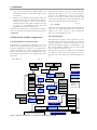
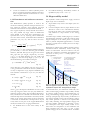
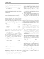
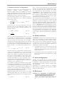
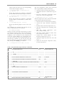
Version 2012-02-08
A model framework for simulating mobilization and movement
of debris flows
based on GRASS
GIS
User manual and model outline
by Martin Mergili
Institute of Applied Geology, BOKU University of Natural Resources and Life Sciences Vienna, Austria
[email protected]
www.mergili.at
February 2012
2 r.debrisflow
r.debrisflow is a GIS-supported model framework for
simulating the potential spatial patterns of debris flow
initiation, movement, and deposition. It is physicallybased in general, but includes some empiricalstatistical components. r.debrisflow is designed as a
raster module for the software GRASS. The scientific
concepts behind r.debrisflow are summarized in
Chapter 1 (Model outline).
In contrast to most of the other GRASS raster modules, management of the data and the parameters (input and output) is not done by adding parameters to
the r.debrisflow command, but by an additional shell
script (r.debrisflow.sh) with various functionalities,
including derivation of secondary input parameters
from primary ones. This is required due to the complexity of the model framework. Instructions how to
operate r.debrisflow are given in Chapter 2 (User’s
manual).
The model shows a large potential for refinements.
Chapter 3 (Prospected improvements) will give a
short overviev of ongoing and prospected further development of r.debrisflow, regarding the scientific
concepts as well as its mode of operation.
Every user is encouraged to report encountered bugs
or errors to
[email protected].
Furthermore, the developer would be grateful for receiving comments regarding
•
experiences with the program, shortcomings,
recommendations for improvements (scientific
concepts, ease of use);
•
parameters chosen for certain study areas;
•
interest in cooperation in application and further
development.
The model, as applicable with GRASS, is running
under the GNU General Public License
(www.gnu.org). r.debrisflow has been created with
the purpose to be useful for modelling of debris
flows. It has been developed with care, and much
emphasis has been put on ensuring its scientific value.
Nevertheless, every user has to be aware that it is only
a computer program created by a human being,
which may contain technical and topical errors and
shortcomings. No responsibility can be taken by the
developer for any types of deficiencies in the program
or in the present document, or for the consequences
of such deficiencies.
___________________________________________________________________________
1 Model outline 3
1.8 References 9
1.1 General aspects 3
2 User’s manual 11
1.2 Hydraulic model components 4
1.2.1 Precipitation and snow melt 4
1.2.2 Interception 4
1.2.3 Evapotranspiration 5
1.2.4 Infiltration 5
1.2.5 Surface runoff 6
2.1 System requirements 11
1.3 Sediment transport model 6
1.3.1 Basic assumptions 6
1.3.2 Detachment and sediment concentration 7
1.4 Slope stability model 7
1.5 Debris flow runout 8
1.5.1 Initiation 8
1.5.2 Routing procedure 8
1.5.3 Runout distance and deposition 9
2.2 Test dataset 11
2.3 File management 11
2.4 Installation 12
2.5 Data management 12
2.5.1 Parameter and data input 12
2.5.2 Preparation of parameters 14
2.5.3 Execution of simulations 15
2.5.4 Post-processing of model output 15
2.5.5 Display of results 16
2.5.6 Removal of result files 17
2.5.7 Cleaning of file system 17
2.5.8 Exit 17
1.6 Model validation 9
3 Prospected improvements 18
1.7 Acknowledgements 9
3.1 Scientific concepts 18
3.2 Ease of use 18
Model outline 3
1 Model outline
1.1 General aspects
The ideas for most of the model components were
taken over from existing models, partly in a modified
form. The model framework was named r.debrisflow
(the r indicates that it is a GRASS raster module). It
was kept relatively simple in its first version presented
here, but was also designed in a way for allowing to
be extended with more sophisticated modules in the
future (compare Chapter 3).
r.debrisflow was implemented using a 2.5D raster
data model (the vertical dimension plays an important
role, but is only quantified by attributes). It combines
physically-based, deterministic modules and modules
based on empirical relationships. r.debrisflow couples
a hydraulic model, a slope stability model, a sediment
transport model, and a debris flow runout model:
•
The deterministic hydraulic model distributes the
water from precipitation or snow melt among
vegetation (interception), soil (infiltration), and
surface (runoff). It then approximates the soil
water status and the runoff variables;
•
the deterministic slope stability model computes
the factor of safety for each cell, based on an infinite slope stability model, and identifies potential starting areas of debris flows;
•
the sediment transport model (based on an empirical approach) provides an estimate for erosion and deposition by surface runoff, allowing
to assess the tendency of bedload-rich runoff to
develop into a debris flow;
•
3: geotechnical mode B: the runoff and sediment
transport models are excluded – like (2), but excluding the influence of runoff on infiltration: for
conditions where it is known that no surface
runoff develops;
•
4: hydraulic mode: the slope stability model is
excluded and only debris flows developing from
sediment-laden runoff are modelled – for conditions where it is known that slope failures play no
role for the mobilization of debris flows;
•
5: fully saturated mode: it is assumed that the entire soil in the study area is saturated. With this
precondition, the slope stability model and the
runout model are computed;
•
6: runout only mode: only the runout model is
computed with defined areas of debris flow initiation – for testing the plausibility of the runout
model for events of known patterns of debris
flow initiation and deposition.
The general model layout is illustrated in Figure 1.
r.debrisflow considers the slope or catchment under
investigation as six-layered system characterized by
the following variables:
•
the overlying atmosphere is described by air
temperature T (degree Celsius) and precipitation
P (m);
•
snow cover is defined as snow depth ds (m);
•
land cover is defined by a raster layer representing nominal land cover classes. Minimum and
maximum values of interception capacity
ICP (m), root cohesion cr (N m-2), and rooting
depth dr (m) have to be assigned to each class.
A hydrological surface class and the width of the
flow channels at a sub-cell scale are defined for
each cell as well as the vegetation surcharge of
Manning’s n nadd;
•
the surface water table is characterized by depth
R (m) and flow velocity vflow (m s-1);
•
soil, here rather understood as sediment cover
than as mixture of residuals from weathering and
decomposed organic matter, is basically represented by a nominal soil class raster layer. A texture class, dry specific weight γ (N m-3), stone
content s (m3 m-3), the hydraulic parameters θr,
θs (m3 m-3), ψ (m) and K (m s-1), and the mechanical parameters soil cohesion cs (N m-2) and
angle of internal friction φ are assigned to each
soil class as well as minimum and maximum values for nbas. Soil depth d (m) is defined independ-
•
the debris flow runout model finally routes the
debris flow downwards to the area of deposition,
based on a two-parameter friction model.
The modules are executed in a defined sequence for a
user-defined number of time steps during and after a
rainfall or snow melt event. Slope stability and runout
are computed at the end of the last time step.
Not all modules have to be executed – the following
combinations (modes of simulation) are possible
when running r.debrisflow:
•
1: full mode: all modules are executed;
•
2: geotechnical mode A: the sediment transport
model is excluded, and only debris flows starting
from slope failures are modelled – for conditions
where it is known that debris flows only develop
from slope failures;
4 r.debrisflow
where ΣM is the daily snow melt (m d-1), and ddf is
the degree-day factor (m °C-1 d-1). Tddf is the temperature in °C at a defined time of the day. In order to
estimate snow melt of shorter time intervals, daily
snow melt is distributed over the considered day, following a linear relationship with temperature:
ently from the soil classes. All parameters are
considered constant over the entire depth of the
soil column;
•
bedrock is considered unconditionally stable. Its
permeability for water is accounted for by the parameter pr, denoting the ratio of total effective
rainfall and snow melt which percolates through
the rock. pr is not defined as raster map, but
globally for the considered study area.
The following sections give a more detailed introduction to the physical and mathematical background of
r.debrisflow.
where T0 is the temperature during the cosidered time
step, ΣT is the daily temperature sum, based on the
length of one time step Δt (s). Only temperatures
above Tcrit are included in the sum.
1.2.2 Interception
1.2 Hydraulic model components
The interception capacity of the vegetation Ipot (m) is
extracted from the land cover dataset. For each time
step Δt (s) rainfall is retained as interception IΔt (m)
until the interception capacity is reached (ΣIΔt = Ipot).
The excess rainfall is added to the soil water table
R (m) as effective rainfall Pr,eff (m).
Water from snow melt is considered not interceptable
by vegetation. This worst-case assumption was chosen due to the often unknown vertical distribution of
Ipot.
1.2.1 Precipitation and snow melt
Precipitation P (m) and air temperature T (°C) are
read from the prepared datasets. Precipitation is considered as rainfall Pr if it exceeds a user-defined temperature threshold Tcrit, usually ranging between 0°C
and 2°C. Snow melt M (m) is computed using a simple degree-day approach with air temperature as the
only input:
Eq. 1,
ΣM = ddf ⋅ Tddf
degree day
factor DDF
air
temperature T
precipitation
P
snow melt S
interception
capacity I
interception I
surface water
depth R
slope α
Manning
roughness n
hydrological
surface class
flow
directions
slope α
grain spec.
weight γ g
Green-Ampt
model
Manning's
formula
flow velocity v
routing
procedure
flow
discharge q
sediment
concentration C
Rickenmann
formula
bedload
discharge q b
Corominas et al (2003)
rules
depth of detachment
or deposition from surface runoff d w
soil hydrological
parameters
s , θr, θs , ψ, K
depth of wetting
front d
soil dry specific
weight γ s
soil cohesion c s
infinite slope
stability model
input
parameter
working
parameter
effective
rainfall P eff
grain size distribution
D30 , D50 , D90
Eq. 2,
M = T0 ΣM ΣT
root cohesion c r
major output
parameter
model
model
in older versions
work flow
(all time steps)
work flow
(last time step)
angle of internal
friction φ
factor of
safety FOS
rooting depth d r
debris flow
volume
test of
criteria
runout distance
potential starting areas
of debris flows
two-parameter
friction model
Rickenmann (1999)
formula
depth of detachment
or deposition from debris flow
Figure 1: General model layout of r.debrisflow. Designed by M. Mergili
runout velocity
loss of elevation
Vandre (1985)
rules
slope α
Model outline 5
depth. For each time step it is tested which case is
applicable:
•
•
•
also the most simple equations for evapotranspiration require highly dynamic parameters that are
usually not available at sufficient accuracy and
resolution (humidity, irradiation, etc.);
R f = R0 − fΔ t short (1 − s )
d = d 0 + Δt short f Δθ
⎞
⎟⎟
⎠
Eq. 4,
where K (m s-1) is the hydraulic conductivity, R0 (m) is
the depth of the surface water table before infiltration, ψ (m) is the matric suction at the wetting front,
and d0 (m) is the depth of the wetting front before
infiltration. Eq. 4 is derived from Darcy’s law
(Xie et al. 2004; Chen & Young 2006). If no measurements of the soil hydraulic parameters are available, values for different texture classes can be obtained e.g. from Rawls et al. (1983) or from Carsel
& Parrish (1988).
Two possible cases have to be distinguished. f has to
be corrected for volumetric stone content s, which
does not affect the maximum possible depth of infiltration, but the volume that fits into the soil until this
case 2: R0 ≤ f Δtshort (1-s) – inflow to the cell is
equal or smaller than maximum possible infiltration capacity. In this case, the entire inflow infiltrates,
d = d 0 + R0 [Δθ (1 − s )]
Eq. 7,
and no surface water table remains, meaning that
no surface runoff will develop from the considered cell.
Eq. 3,
infiltration limited by
infiltration capacity
V inf < V surf
old wetting front
where Rprev is the depth of the surface water table at
the end of the previous time step. The infiltration of
water into the soil is a complex process influenced by
an interplay of factors like the depth of the surface
water table, the soil parameters, and the local topography. It was chosen to use the Green & Ampt (1911)
approach, assuming a sharp wetting front as the interface between saturated soil above and soil at initial
moisture content below (Figure 2). The hydraulic parameters governing infiltration are derived from the
grain size class of the soil. Infiltration capacity f (m s1) can be stated as
⎛ R +ψ
f = K ⎜⎜1 + 0
d0
⎝
•
potential depth of infiltration
Δtshort
(Peff ,t + M t )
Δt
Eq. 6,
where Δθ is the moisture deficit of the soil (difference between saturated water content θs and
initial water content θi; all in m3 m-3);
1.2.4 Infiltration
R0 = R prev +
Eq. 5,
Infiltration is limited by the infiltration capacity,
and the depth of the new wetting front d (m) is
computed as follows:
the model is designed primarily for short and intense rainfall events, where evapotranspiration is
rather negligible. Regarding snow melt, neglect of
evapotranspiration may lead to more significant
inaccuracies.
Infiltration, runoff, and sediment transport have to be
calculated at much shorter time steps Δtshort than the
other processes, meaning that the entire sequence has
to be repeated for various times within each basic
time step Δt. Δtshort is determined according to Eq. 14.
The water input from effective rainfall and the snow
melt are added to the surface water table of the cell at
the beginning of each short time step:
case 1: R0 > f Δtshort (1-s) – inflow to the cell exceeds maximum possible infiltration and depth of
surface water table after infiltration Rf (m) is expressed as
V surf
infiltration limited by
surface water table
V inf = V surf
surface
water
table
V surf
V inf
V inf
∆Θ (1-s )
∆Θ (1-s )
already saturated soil
Potential evapotranspiration Epot (m) is set to zero.
This is a worst-case assumption again which was chosen for two reasons:
new saturated soil
1.2.3 Evapotranspiration
soil at initial
moisture content
Figure 2: Infiltration into the soil according to the Green
& Ampt (1911) model, as applied for the present study.
Vsurf = volume of surface water before infiltration,
Vinf = infiltrated volume. Designed by M. Mergili.
For case 1, s has no direct influence on d, for case 2, d
increases with increasing s. The application of this
method has to be considered as an approximation:
•
The Green-Ampt approach, in its strict sense,
was developed for horizontal surfaces, but is also
applied for slopes. Chen & Young (2006) showed
that on slopes until 45°, the effect of slope angle
is small, compared to other sources of inaccuracy;
•
stone content is not accounted for in the original
model. Therefore it was decided to disregard its
influence on infiltration capacity, but its role as
6 Model outline
limiting the infiltrable volume was taken into account. More research would be necessary in order to clarify the inaccuracies connected to this
simplification.
Slope-parallel seepage is neglected in the model. The
infiltration is computed separately for soil below flow
channels and soil in between flow channels. In between flow channels, ΣIF and OF are zero (compare
Eq. 13 and 14).
The integral form of the Green-Ampt approach
(compare e.g. Xie et al. 2004) is not used as the model
is run in short time steps with varying rainfall intensities.
slopes, inaccuracies of the DEM or landforms on
a sub-cell scale may exert a stronger effect on
flow direction than on steep slopes.
For both cases, inflow ΣIF (m) is computed with the
Manning formula in the same way:
vf low =
1
nman
R f 3 (sin α )2
2
1
Eq. 8,
where α is the local slope angle in degrees and nman is
the surface roughness (determined by vegetation, soil
texture, and obstacles), which is computed using
nman = m(nbas + nsdd )
Eq. 9,
where m is a factor accounting for meandering, nbas is
the basic n value, and nadd is a surcharge for vegetation, obstacles, etc. m is automatically set to 1.0 since
the model presented here is designed for steep terrain
with poor meandering of the channels.
The water discharge per unit width q (m2 s-1) is computed as follows:
q = v flow R f =
5
1
1
R f 3 (sin α )2
n man
Eq. 10.
v flow Δtshort
i =1
d h,i
i=n
1
i =1
nman ,i
=∑
1
Δt short 3
R f ,i (sin α i )2
d h ,i
5
Eq. 12,
where n is the number of contributing upslope cells,
dh,i (m) is the horizontal distance between the centre
of the cell i and the centre of the considered cell.
Outflow OF (m) is computed in an analogous way:
1.2.5 Surface runoff
After computing infiltration, the ponded water of the
depth Rf is assumed to concentrate in the flow channels immediately and to run off superficially. Strictly
spoken, Rf = Aflow/Pwet, where Aflow (m²) stands for the
cross section of the flow, and Pwet (m) is the wetted
perimeter, but in the model, Rf is approximated by
flow depth. Runoff velocity vflow (m s-1) is computed
using the Manning formula:
i=n
ΣIF = ∑ R f ,i
OF = R f
v flow Δt short
Eq. 13,
dh
where dh (m) stands for the horizontal distance between the centre of the considered cell and the centre
of the downslope cell. The length of one short time
step Δtshort (s) is defined as
Δtshort = a d cell vmax
Eq. 14,
where a is a factor ≤ 1 set to 0.5, dcell (m) is the cell
size and vmax (m s-1) is the maximum runoff velocity
over the entire area. Too short time steps would unnecessarily increase computing time. Δtshort is defined
by the program automatically according to Eq. 14,
using the maximum flow velocity of the previous
time step over all cells. Δtshort is set to 20 s if
dcell/vmax exceeds a threshold value. If no runoff occurs at all, Δtshort is set to 120 s.
The depth of the water table R for each cell is computed as follows:
R = R f + T + M + ΣIF − OF
Eq. 15,
where T is the effective rainfall, M is the snow melt,
ΣIF stands for the total inflow from all the upslope
cells directly draining into the considered cell, and OF
stands for the outflow (all values in meters).
Surface runoff is computed separately for each hydrological surface class HSC:
1.3 Sediment transport model
•
1.3.1 Basic assumptions
•
HSC = 1 (defined channel): the water is routed
through the channel, with only one possible
downward direction from each cell;
HSC = 2 (slope with numerous small channels or
no channels at all): the water is routed downwards assuming the defined channel densities on
a sub-cell scale and a random walk weighted for
slope angle:
w=α
u1
Eq. 11,
where w is the weight assigned to each potential
flow direction and u1 is a user-defined exponent
(values of 3 to 4 appear reasonable) – on gentle
Surface runoff, independently of occurring as overland flow or channel flow, has a certain capacity to
transport sediment. If the actual load is below transport capacity, soil from the bed is eroded, whilst
sediment is deposited in the reverse case. The following assumptions are set in the model:
•
only bedload is considered as relevant regarding
the magnitude of sediment transport and the
evolution of debris flows. Suspended load is neglected;
Model outline 7
•
runoff is considered to follow hydraulic principles to a certain threshold of sediment concentration; at higher sediment concentrations it is considered as debris flow.
•
the bedload discharge immediately reaches an
equilibrium (only if ST3 = ST4 = 1).
1.4 Slope stability model
1.3.2 Detachment and sediment concentration
The hydraulic model components supply saturated
depth d (m). It is assumed that
The Rickenmann (1990) equation is used in the
model for estimating sediment transport because it is
best suited for relatively steep channels and high
sediment concentrations. It only includes bedload.
The original equations, mainly derived from laboratory tests, yielded very high values of detachment
when applied to the study areas. Furthermore, the
equation does not say anything about detachment
rates. For these reasons, the dimensionless calibration
parameters ST1, ST2, ST3, and ST4 had to be introduced:
•
qb = ST1
12.6 ⎛ D90 ⎞
⎜
⎟
(s − 1)1.6 ⎝ D30 ⎠
0.2
(q − qcr )(sin α )2 Eq. 16,
where qb (m2 s-1) is the volumetric bedload transport
per unit width, s is the ratio between grain and fluid
densities, D90 and D30 (m) are the grain sizes where
90% and 30% per weight, respectively, are finer,
q (m2 s-1) is the fluid discharge per unit width, and
α (degree) is the local slope angle. qcr (m2 s-1) is the
threshold discharge for sediment transport:
qcr = ST2 0.065(s − 1)
1.67
0.5
1.5
g D50
(sin α )
−1.12
Eq. 17,
slope failures only occur at the depth d (the wetting front);
•
if total soil depth is known, slope failures are also
allowed to occur at the soil-bedrock interface,
but only if the entire soil is saturated (mathematically identical to slope failures at the wetting
front).
An infinite slope stability model (Figure 3) is used for
the calculations. Therefore a wide ratio between slope
length and depth of the failure plane is required in
order to yield an acceptable approximation – a condition that is usually met for shallow, but not for deepseated failures.
Furthermore, infinite slope stability models assume a
translational failure mechanism, which usually only
occurs in cohesionless soils. For cohesive soils, the
model may still derive reasonable approximations of
the factor of safety, but is – strictly spoken – not
really applicable.
γ ‘ = submerged unit weight
γ w = unit weight of water
G ‘ = weight of moist soil
N = normal force
T = shear force
F s = seepage force
T f = shear restistance force
Eq. 18,
d w = ST4 (l0 − qb v ) for l0 > qb v
Eq. 19,
l = l0 − d w = qb v
Eq. 20,
C = l (l + R )
Eq. 21,
•
R
FOS = Tf / (T + F s )
d
FOS > 1: cell is stable
FOS < 1: cell is pot. unstable
T
the bedload moves at the same velocity as the
water;
Fs
α
N
where l0 (m) is the depth of bedload at the start of the
time step. Negative values of dw (Eq. 18) indicate detachment, positive values (Eq. 19) indicate deposition.
Only saturated soil is allowed to be detached. All the
sediment deposited is considered as saturated, and the
depth of the wetting front below the flow channel(s)
is corrected for detachment and deposition. Eq. 18
to 20, which are not part of the original Rickenmann
model, are based on two rough generalizations:
G‘ = γ ‘ ∆x d
N = G ‘ cos α
T = G ‘ sin α
F s = ∆x d γ w sin α
T f = N‘ tan φ + c ∆x / cos α
where D50 (m) is the median grain size, and g (m s-2)
is the gravitational acceleration. Erosion (detachment
of soil) or deposition dw (m), depth of bedload l (m),
and sediment concentration C (m3 m-3) can then be
derived:
d w = ST3 (l0 − qb v ) for l0 < qb v
R = ponding depth (hydr. radius)
d = depth of potential failure
plane = depth of wetting front
G‘
∆x
γ‘
γd
Figure 3: Mechanisms for infiltration and shallow slope
failure as applied in the present study. For a detailed
explanation compare text. Designed by M. Mergili.
As discussed above, the infiltration model only considers vertical seepage. Infinite slope stability models,
in contrast, usually assume a slope-parallel flow, exerting a destabilizing seepage force Fs (N) parallel to
the slope (compare Eq. 29). In reality, the direction of
the seepage depends on the local conditions, particularly on the presence or absence of an impermeable
layer. Fully including the slope-parallel seepage into
the slope stability calculations is therefore a worstcase assumption. The slope stability model is executed after the computation of the infiltration has
been completed (last time step), so that a slopeparallel seepage can be assumed without contradic-
8 Model outline
least one time step are considered to fail at the
deepest failure plane identified for the cell during
the event. Failed soil with a sediment concentration of Csoil < Cmax, where Csoil = 1-θ(1-s), is considered to evolve into a debris flow. In reality,
debris flows with higher sediment concentration
do occur, particularly in non-cohesive soils. The
model therefore assumes that all failed soil with
cs = 0 develops into a debris flow also at at higher
sediment concentrations;
tion to the vertical seepage computed with the GreenAmpt model.
The dimensionless factor of safety FOS is stated as
FOS = T f
(T + Fs )
Eq. 22,
where Tf is the shear resistance force of the soil, T is
the shear force, and Fs is the seepage force (all in N;
compare Figure 3). Shear resistance s (N m-2) follows
Coulomb’s law:
s = c + σ (tan ϕ )
Eq. 23,
and the corresponding shear resistance force is
T f = N ' tan ϕ + c ⋅ Δx cos α
Eq. 24,
where N is the normal force, φ (degree) is the angle
of internal friction, c (N m-2) is the cohesion (soil cohesion cs plus root cohesion cr), Δx (m) is the length
of the considered slope segment in downslope direction, and α (degree) is the slope angle. N and T (N)
are computed from the weight of the moist soil
G’ (N):
G ' = γ '⋅Δx ⋅ d
Eq. 25,
N = G ' cos α
Eq. 26,
T = G' sin α
Eq. 27,
where γ’ (N m-3) is the specific weight of saturated
soil and d (m) is the depth of the potential failure
plane:
γ ' = γ d + γ w [θ s (1 − s ) − 1]
Eq. 29.
Dry and cohesionless soils (Fs = 0; c = 0; γ’ = γd) are
stable when α < φ, and unstable when α > φ.
The forces exerted by the surface water table R (m)
are neglected in the model.
1.5 Debris flow runout
1.5.1 Initiation
Debris flows are supposed to occur within a certain
range of sediment concentrations, usually between
Cmin = 0.45 and Cmax = 0.55.
•
for every cell where runoff is modelled to evolve
into a debris flow, sediment concentration C is
tested against Cmin after each time step. If
C > Cmin, the material is retained from sediment
load. All retained material is routed downslope as
debris flow at the end of the last time step.
Before routing the debris flow downwards, the volume and the size of each patch of cells of potential
debris flow initiation are calculated. If one of these
variables or the depth of potential initiation is below
user-defined thresholds, the patch or the cell, respectively, is excluded from runout.
1.5.2 Routing procedure
The debris flow is not simply routed downwards the
steepest slope. Similar to surface runoff, the routing
algorithm is determined by the hydrological surface
class:
•
HSC = 1 (defined channel): the debris flow is
routed through the channel with only one possible downward direction from each cell. As soon
as deposition occurs in a channel, the corresponding cells are considered as HSC = 2 for the
further simulation;
•
HSC = 2 (no clearly defined channel): a random
walk weighted for downslope angle is applied for
routing the debris flow. The weight w is determined automatically as a function of the steepest
slope. It is expressed as:
Eq. 28.
γd is the specific weight of dry soil, and γw is the specific weight of water (both in N m-2). γd is derived
from grain specific weight (to be specified by the
user; 26.5 kN m-3 for quartzitic material), and θs and s
as surrogates for pore volume.
The seepage force exerted by the soil water is stated
as
Fs = Δx ⋅ d ⋅ γ w sin α
•
At the end of the last time step, all cells identified
as potentially unstable (with FOS < 1) during at
w = α u 2 β u 2 −1
Eq. 30,
where the exponent u2 has to be specified by the
user (values between 3 and 5 appear reasonable).
β (degree) is the slope angle where deposition
starts (compare below; w = 0) for upslope angles.
Similar to runoff, this algorithm accounts for the
higher tendency of debris flows to take another
than the steepest slope specified in the DEM on
gentle slopes than on steep slopes.
Each cell containing starting material for a debris
flow is passed through the routing procedure individually. Routing continues until the debris flow has
stopped, according to the criterion specified in the
next section.
Model outline 9
1.5.3 Runout distance and deposition
Runout is computed using a semi-deterministic twoparameter
friction
model
developed
by
Perla et al. (1980) which was modified by Gamma
(2000) and applied by Wichmann (2006) in a rasterbased GIS environment. It is not only applicable to
debris flows, but also to snow avalanches.
The deterministic element of the approach is the velocity of the debris flow v (m s-1) which is computed
for each raster cell i:
(
)
⎛M ⎞
vi = ζ i ⎜ ⎟ 1 − eη i + vi2−1eη i cos(Δα i )
⎝ D ⎠i
Eq. 31,
where M/D (m) is the mass-to-drag ratio of the debris flow, and vi-1 is the debris flow velocity of the
previous cell. The factor ζi and the coefficient ηi are
derived as follows:
ζ i = g (sin α i − μ cosα i )
ηi =
− 2 Li
(M / D )i
Eq. 32,
Eq. 33,
where g is gravitational acceleration (9.81 m s-2 on the
earth surface), αi is local slope angle, μ is the dimensionless friction coefficient, and L (m) is slope length
(cell size corrected for slope angle). ∆α is the difference between the slope angle of the previous cell and
the slope angle of the considered cell which is set ot 0
for convex slopes or channels (Wichmann 2006). For
concave slopes, vi-1 is corrected as the flow loses energy:
v1−1 = vi −1,0 cos(α i −1 − α i ) if αi-1 > αi
1.6 Model validation
r.debrisflow is mainly based on physically based concepts, but nevertheless it contains empirical elements
and an array of parameters some of which are difficult to measure or to estimate. Therefore some type
of calibration of some of the parameters is required
for each study area. For this purpose, datasets for
validation are needed, for example:
•
if the debris flows hit a road: records by the road
authorities about volumes to be removed after
debris flow events connected to known meteorological conditions; or
•
the distribution and extent of landslide scars and
patterns of deposition from debris flows visible
in the field.
Eq. 34.
The first term in Eq. 31 determines if the flow accelerates (ζ > 0) or decelerates (ζ < 0), the second term
provides the contribution of flow velocity to the final
velocity. M/D, being a surrogate for the inertia of the
flow, exerts a major influence on flow velocity, while
its impact on runout distance is small. The latter is
primarily determined by the topography and μ
(Gamma 2000; Wichmann 2006). The simulation is
stopped as soon as vi becomes undefined (square root
of negative value, compare Eq. 31).
One problem regarding the calibration of this model
is that different combinations of the two parameters
to be calibrated (M/D and μ) may result in the same
runout distance. A common way for calibration is
therefore to set M/D to values leading to realistic velocities, and then calibrating μ in order to correlate
simulated and observed runout distances.
Wichmann (2006) used values of M/D = 75 m. The
following relationship for μ was found to be useful
for computing the maximum runout length (Gamma
2000):
μ = 0.13 A−0.25
where A (km²) is the catchment size for the considered cell. It is assumed that μ would decrease with increasing A because the water content of the debris
flow would increase. This relationship was used in
r.debrisflow, but with user-defined factor and exponent in order to allow calibration for other conditions. Following Gamma (2000), the range of values
of μ would be restricted to a maximum of 0.3 and a
minimum of 0.045, overruling Eq. 35.
The two-parameter friction model does not say anything about the patterns of particle entrainment and
deposition. Instead of designing a more complex
scheme like Wichmann (2006), simple thresholds of
slope and velocity are used for delineating these processes in r.debrisflow, where entrainment (as far down
as to the wetting front) is only assumed if both parameters are above the threshold, whilst deposition is
assumed to take place only if both parameters are below the thresholds. The calibration of the thresholds
is connected to the same problems as the calibration
of M/D and μ (different combinations of parameter
values).
Eq. 35,
1.7 Acknowledgements
Funding was provided by the Tyrolean Science
Funds, the Vice Rector for Research of the University
of Innsbruck (“Doktoratsstipendium aus der Nachwuchsförderung der LFU”), and the Austrian Academy of Sciences.
Furthermore, the valuable remarks of Wolfgang
Fellin (Institute of Infrastructure, University of Innsbruck) are acknowledged.
1.8 References
Arcement, G.J. & Schneider, V.R. (2000): Guide
for Selecting Manning's Roughness Coefficients for Natural Channels and Flood
Plains. USGS Water-supply Paper 2339. 67
p.
10 Model outline
Carsel, R. F. & Parrish, R. S. 1988: Developing
joint probability distributions of soil water retention characteristics. Water Resources
Research 24: 755-769.
Chen, L. & Young, M.H. (2006): Green-Ampt infiltration model for sloping surfaces. Water
Resources Research 42. 9 p.
Gamma, P. 2000: dfwalk – Ein MurgangSimulationsprogramm zur
Gefahrenzonierung. Geographica Bernensia
G66, 144 pp. In German.
Green,W.H. & Ampt, G.A. (1911): Studies on soil
physics. Journal of Agricultural Sciences 4:
1-24.
Perla, R., Cheng, T.T. & McClung, D.M. 1980: A
Two-Parameter Model of Snow Avalanche
Motion. Journal of Glaciology 26: 197-207.
Rawls, W.J., Brakensiek, D. L. & Miller, N. 1983:
Green-Ampt infiltration parameters from soil
data. Journal of Hydraulic Engineering 109:
62-70.
Rickenmann, D. (1990): Bedload transport capacity of slurry flows at steep slopes.
Mitteilungen der Versuchsanstalt für
Wasserbau, Hydrologie und Glaziologie,
ETH Zürich, Nr. 103. 249 p.
Rickenmann, D. (1999): Empirical Relationships
for Debris Flows. Natural Hazards 19: 47-77.
Wichmann, V. 2006: Modellierung
geomorphologischer prozesse in einem
alpinen Einzugsgebiet. Abgrenzung und
Klassifizierung der Wirkungsräume von
Sturzprozessen und Muren mit einem GIS.
Eichstätter Geographische Arbeiten 15.
231 pp. In German.
Xie, M., Esaki, T. & Cai, M. 2004a: A time-space
based approach for mapping rainfall-induced
shallow landslide hazard. Environmental
Geology 46: 840-850.
User’s manual 11
2 User’s manual
2.1 System requirements
r.debrisflow was developed and tested under Fedora
Core 6 with GRASS 6.2.1. It probably works on most other UNIX systems as well as with other versions
of GRASS. The module itself should also be usable
under cygwin, but the related shell script
r.debrisflow.sh (compare below) would probably not
work.
Please make sure to have a proper installation of
GRASS before installing r.debrisflow. In case of
doubt, please consult www.grass.itc.it.
2.2 Test dataset
A test dataset is provided together with the program,
consisting of some text files and a GRASS location
with the name test_rdebrisflow. All data is packed in
the file test_rdebrisflow.zip.
test_prec.txt and test_temp.txt contain precipitation
and temperature data in the format described below,
while test_param.txt is the required parameter file.
test_ctrlpoints.txt contains the control points (compare below). Table 1 shows the names of the raster
and vector maps.
Table 1: Names of the maps of the test dataset
name of the map
description
test_mask
test_elev
mask for study catchment (raster)
elevation map at 5 m resolution
(raster)
elevation map at 10 m resolution
(raster)
soil classes (raster)
soil depth (raster)
land cover classes (raster)
hydrological surface classes at 5 m
resolution (raster)
hydrological surface classes at
10 m resolution (raster)
width of flow channel(s) at 5 m
resolution (raster)
width of flow channel(s) at 10 m
resolution (raster)
road (object at risk; raster)
depth of snow cover (raster)
predefined depth of debris flow
initiation (raster)
predefined maximum depth of entrainment (raster)
observed patterns of debris flow
initiation (line vector)
observed patterns of deposition
from debris flow (line vector)
reclass tables described below are suitable for the soil
and land cover classes in the test dataset – for other
datasets, they have to be modified.
2.3 File management
The file system behind r.debrisflow consists of two
parts:
•
a GRASS mapset with all the spatially distributed
input information as raster or vector maps, and
•
a folder named r.debrisflow, which may be stored
at any location in your home directory. The internal structure of the folder r.debrisflow may not
be manipulated, otherwise some of the functionalities will fail.
The directory r.debrisflow contains the following subdirectories:
tools
The tools directory hosts the scripts required for installing and running r.debrisflow:
•
main.c: the source code for r.debrisflow;
•
r.debrisflow.sh: a shell script facilitating data input, management, and output (compare below);
•
install.sh: a shell script helping to compile the
source code (main.c).
data
test_elev10
test_soilclass
test_soildepth
test_landcover
test_hydcl
test_hydcl10
test_chanw
test_chanw10
test_road
test_snowdepth
test_dinitdef
test_dscourdef
test_init_observed
test_depd_observed
The test dataset is suitable to run r.debrisflow at spatial resolutions of 5 m or 10 m. Please note that the
It contains the input files of the meteorological data,
the parameter file, and the file with control points
(compare below), and a file for scaling the legends of
the resulting maps to be displayed. The subfolder
/recl contains reclass tables (for deriving secondary
parameters from input datasets), the subfolder
/colors contains colour tables for display.
temp
The temp directory contains temporary files created
during the execution of r.debrisflow.sh. Its content
shall not be manipulated manually, but only using the
functionalities of r.debrisflow.sh.
results
It contains some simulation results (summary file,
documentation file; compare below). However, the
main results are stored as rasters in the active GRASS
mapset.
docs
The docs directory contains this manual.
12 Appendix 3: Manuals
2.4 Installation
•
Boolean raster map defining the catchment of interest (identified by cell values of 1, areas out of
the catchment are defined by 0 or no data).
r.debrisflow has to be added to the GRASS raster li-
brary as a new module, based on the source code of
the file main.c. For performing this task, log in as super user (su). call the script install.sh in the folder
r.debrisflow/tools:
cd dir/r.debrisflow/tools
sh install.sh
dir may be any location in your
following prompt is displayed:
•
•
Here, enter the path to the GRASS source, for example
The Makefile is created, and compilation and installation are run automatically, so that r.debrisflow is
ready to use.
Please note that you have to change to the tools directory as described above – if just entering
•
2.5 Data management
r.debrisflow uses text files and rasters with predefined
names as input. The shell script r.debrisflow.sh serves
for creating these datasets, and for generating secondary datasets from primary information (e.g. hydraulic
conductivity from grain size class). It must be run
from within the used GRASS mapset:
cd dir/r.debrisflow/tools
sh r.debrisflow.sh
r.debrisflow.sh offers the following modules:
-->
-->
-->
-->
-->
-->
-->
-->
Parameter and data input
Preparation of parameters
Execution of simulations
Post-processing of model output
Display of results
Removal of result files
Cleaning of file system
Exit
By entering a number, the corresponding module is
executed.. The modules are described in detail below.
r.debrisflow.sh has to be called from within the
GRASS mapset with all the required raster maps.
•
data and parameters. If no input is given for a prompt
(by just pressing ENTER), the dataset specified earlier
is kept. The numbers behind the prompts denote the
modes of simulation (compare Chapter 1) for which
the corresponding dataset is required.
--> Objects at risk map (boolean):
|1|2|3|4|5|6|
Boolean raster map denoting objects at risk (1
for presence of potential objects at risk like roads
or buildings, else 0 or no data).
•
--> Soil classes map (integer):
|1|2|3|4|5|
Integer raster map with predefined soil classes
(compare Module 2: Preparation of parameters).
The numbers of the classes may be chosen freely,
but must fit to the corresponding reclass tables
(compare Table 3).
2.5.1 Parameter and data input
Module 1 consists of a sequence of prompts for input
--> Channel width map: |1|2|3|4|5|6|
Raster map denoting total width of flow channel(s) for each cell, connected to the hydrological
surface classes: 1 (defined flow channel): width
of the flow channel; 2 (multiple channels or unconcentrated overland flow): ratio between sum
of width of all flow channels crossing a cell and
cell width, perpendicular to the steepest slope.
The advantage of this approach is to be largely
independent from cell size, at least for quite uniform distributions of channels.
Also here, the cell size has to correspond to the
cell size of the simulation it shall be used for.
Additionally, it has to fit to the hydrological surface classes map exactly in order to avoid serious
problems during simulation.
an error message will display and r.debrisflow will not
be installed.
1
2
3
4
5
6
7
8
--> Hydrological surface classes map (integer): |1|2|3|4|5|6|
Integer raster map of the distribution of the hydrological surface classes (1 for defined flow
channel, 2 for multiple flow channel or unconcentrated overland flow). Care has to be taken
that the cell size of the map corresponds to the
cell size of the simulation it shall be used for.
Particularly the defined channels (class 1) have to
be clean and continuous.
/usr/local/src/grass64_release/
sh dir/r.debrisflow/tools/install.sh
--> Soil depth map (m): |1|2|3|4|5|6|
Raster map of soil depth (in meters). If soil depth
is not known, it should be set to a high value. For
bedrock, it has to be set to 0.
directory. The
Full path to GRASS source (slashes at beginning and end):
--> Elevation map (m): |1|2|3|4|5|6|
Raster map of elevation (meters).
•
home
--> Catchment map (boolean): |1|2|3|4|5|6|
•
--> Land cover classes map (integer):
|1|2|3|4|
Integer raster map with predefined land cover
classes (compare Module 2: Preparation of parameters). The numbers of the classes may be
User’s manual 13
chosen freely, but must fit to the corresponding
reclass tables (compare Table 3).
•
File with precipitation values (from measured
data or hypothetical). header information:
o first line: elevation of rain gauge (meters);
o second line: duration of basic time step (seconds);
o third line downwards: precipitation values
(mm), sum of one time step per line.
--> Estimated depth of mobilization of
soil map (m): |6|
Raster map showing the patterns of estimated
potential debris flow initiation (depth in meters).
•
--> Estimated depth of entrainment of soil
map (m): |5|6|
Raster map showing the patterns of estimated
potential depth of entrainment by debris flows
(meters).
•
--> Snow depth map (m): |1|2|3|4|
Raster map denoting depth of snow cover (meters).
The remaining four required input datasets are the
names of files which have to exist in the
dir/r.debrisflow/data
directory. In each of the files, each line has to consist
of a label (first column) and a value (second column).
The content of the label only serves for enhancing
readability, it has no influence on the simulation, but
it may not contain tabulators. It is important, however, that it does exist and is separated from the actual value by a tabulator, as only the part of the file
after the tabulator is used. Please consult the example
files (starting with example_) as reference.
•
•
--> Temperature file (°C): |1|2|3|4|
File with temperature values (from measured data
or hypothetical). Header information:
o first line: elevation of thermometer (meters);
o second line: daily minimum temperature
(°C);
o third line: daily maximum temperature (°C);
o forth line: temperature for computing snow
melt (°C);
o fifth line: critical temperature (rainfall/snowfall boundary, °C);
o sixth line: vertical gradient for daily minimum temperature (°C m-1);
o seventh line: vertical gradient for daily
maximum temperature (°C m-1);
o eighth line: degree day factor for snow melt
(m °C-1).
o Ninth line downwards: temperature values,
one time step per line.
--> Precipitation file (mm): |1|2|3|4|
Table 2: Input parameters (single values) for r.debrisflow
variable
γg
u1
u2
–
–
–
–
M/D
–
–
–
–
description
unit
-3
grain specific weight of soil
Nm
exponent for weighting of slope angle for surface runoff random walk exponent
exponent for weighting of slope angle for debris flow runout random exponent
walk
percolation through rock (ratio compared to effective rainfall plus
ratio
snow melt)
factor for calibration of critical runoff formula
factor
factor for calibration of potential sediment load formula
factor
factor for calibrating detachment by surface runoff
factor
factor for calibrating deposition from surface runoff
minimum sediment concentration for development of debris flow
ratio
maximum sediment concentration for development of debris flow in ratio
cohesive soil
minimum depth of unstable or detached soil for initiation of debris flow m
minimum number of adjacent failed cells for development of debris
integer
flow
minimum volume of unstable or detached soil for development of de- m³
bris flow
factor for computing μ (compare Eq. 35)
factor
exponent for computing μ (compare Eq. 35)
exponent
lower threshold for μ
coefficient
upper threshold for μ
coefficient
mass-to-drag ratio
m
slope threshold for entrainment/deposition
deg
1
velocity threshold for entrainment/deposition
m smaximum depth of debris flow deposit
m
options for distribution of material deposited from debris flow
integer
–
Minimum slope angle for initiation of debris flows
pr
ST1
ST2
ST3
ST4
Cmin
Cmax
–
–
–
deg.
examples of value(s)
26,500 for quartzitic soil
3
4
0.0–1.0
1.0
0.005 – 0.01
0.1 cell sizes
factor
0.45
0.55
various
depends on cell size
various
0.13
-0.25
0.045 – 0.15
0.3
75
15
10
5 – 15
1 for wedge-shaped towards
the front, 2 for even
20 – 30
14 Appendix 3: Manuals
Table 3: Spatially distributed input parameters of r.debrisflow, specified in Module 1 or automatically created in
Module 2 of r.debrisflow.sh, respectively
shortcut
description
catchment
elevation
soildepth
soilclass
landcovclass
hsc
chanwidth
riskobj
dinitdef
dscourdef
snow
soil
alpha
my
icp
croot
definition of catchment of interest
boolean
elevation above sea level
m
depth of soil
m
class of soil
integer
class of land cover
integer
hydrological surface class
integer
width of flow channel
m, ratio
definition of objects potentially at risk boolean
depth of debris flow initiation
m
maximum depth of entrainment
m
depth of snow cover
m
presence of soil
boolean
local slope angle
deg.
friction coefficient for runout
coeff.
interception capacity of the vegeta- m
tion
-2
root cohesion
Nm
droot
rooting depth
m
nman_add
vegetation surcharge for Manning’s n
texture class of soil
d30 grain diameter of soil
d50 grain diameter of soil
d90 grain diameter of soil
skeleton content of soil (> 2 mm)
dry specific weight of soil
soil cohesion
soil angle of internal friction
basic value for Manning’s n
summand
factor for preferential (macropore)
flow, to be multiplied with infiltration
capacity
soil residual water content
soil saturated water content
matric suction at wetting front
soil hydraulic conductivity
factor
textclass
d30
d50
d90
skeleton
gammad
csoil
phi
nman_bas
pref
thetar
thetas
psi
k
unit
ratio
ratio
m
-1
ms
--> Parameter file: |1|2|3|4|5|6|
File with list of parameters for simulation, one
per line. The parameters have to be specified in a
defined order (Table 2).
In the folder dir/r.debrisflow/data/, a file
with example parameters (example_param.txt) is
provided.
•
Module 1
soildepth
elevation
landcovclass
integer
soilclass
m
m
m
ratio
-3
Nm
-2
Nm
deg.
summand
Temperature is only relevant when including
snow melt or when it is lower than the critical
temperature separating rainfall and snow fall. If
the raster map of snow depth is 0 m over the entire catchment, the specified values have no influence on the results of the simulation as long as
the exceed the critical temperature.
•
derived
name of reclass table
from
dir/r.debrisflow/data/recl/
specified as
input in
textclass
recl_lcv_icp4_min.txt
recl_lcv_icp4_max.txt
recl_lcv_croot_min0.txt
recl_lcv_croot_max0.txt
recl_lcv_droot_min1.txt
recl_lcv_droot_max1.txt
recl_nman_add_min3.txt
recl_nman_add_max3.txt
recl_soil_class0.txt
recl_soil_d305.txt
recl_soil_d505.txt
recl_soil_d905.txt
recl_soil_s3.txt
recl_soil_gammad0.txt
recl_soil_c0.txt
recl_soil_phi1.txt
recl_nman_bas_min3.txt
recl_nman_bas_max3.txt
modes of simulation
1 2 3 4 5 6
x x x x x x
x x x x x x
x x x x x x
x x x x x
x x x x x
x x x x x x
x x x x x x
x x x x x x
x
x x
x x x x
x x x x x x
x x x x x x
x x x x x x
x x x x
x
x
x
x
x
x
x
x
x
x
x
x
x
x
x
x
x
x
x
x
x
x
x
x
x
x
x
x
x
recl_soil_pref_min1.txt
recl_soil_pref_max1.txt
x
x
x
x
recl_hyd_thetar3.txt
recl_hyd_thetas2.txt
recl_hyd_psi5.txt
recl_hyd_k9.txt
x
x
x
x
x
x
x
x
x
x
x
x
x
x
x
x
x
x
x
x
x
x
x
x
x
x
x
x
x
x
x
x
x
x
provided. The order shown in this file has to be
kept for all legend files
•
--> File with coordinates of control
points: |1|2|3|4|
File with coordinates of some specific points for
which some variables are documented for each
time step. Each line contains one coordinate –
first line the x coordinate of the first point, second line the y coordinate of the first point, third
line the x coordinate of the second point, etc.
Please note that, if you do not wish to specify
control points, the file has to exist, anyway (otherwise, r.debrisflow will produce an error message), but may be empty.
--> Legend file: |1|2|3|4|5|6|
2.5.2 Preparation of parameters
File with user-specified values serving as maxima
for the display of the output maps.
In the folder dir/r.debrisflow/data/, an example for a legend file (example_legend.txt) is
No user inputs are required for this module, which
serves for the automatic derivation of secondary input parameter maps from the maps specified in Module 1. A slope raster map is derived from the eleva-
User’s manual 15
tion model (r.slope.aspect), and a boolean presence
of soil map is derived from the soil depth map. Secondary parameter maps are derived from the land
cover and soil classes using reclass tables (compare
Table 3; r.reclass). All the reclass tables have to be
stored under
dir/r.debrisflow/data/asc/
and must exactly be named as shown in Table 3. All
the reclass tables must correspond to the following
pattern:
original value_1 = derived value_1
original value_2 = derived value_2
...
original value_n = derived value_n
end
for example
1 = 34
3 = 5
...
10 = 37
end
All numbers must be left-aligned and all equal signs
have to stand in one column.
The numbers before the .txt extension of the reclass
files denote the factor with which the original derived
values have to be multiplied before writing them into
the reclass table. This is necessary because the
r.reclass module of GRASS is not able to cope with
non-integer values. After reclassification, the magnitude of the derived raster maps is corrected automatically.
For parameters with max or min at the end of the
name of the reclass table, the pixel values of the created raster map are randomly distributed between the
minimum and the maximum values. If this is not desired, the maxima and minima have to be identical.
Example reclass tables are stored in the abovementioned directory, but the tables have to be modified
for each study area, except the tables for the hydraulic
parameters, which refer to grain size classes according
to the following key: 1=S; 2=LS; 3=SL; 4=SCL;
5=SC; 6=L; 7=CL; 8=SIL; 9=C; 10=SICL; 11=SI;
12=SIC.
It is possible to skip Module 2 and instead create all
the parameter maps manually. In this case, please
note that the naming conventions have to be met exactly in order to ensure the functionality of the simulation (compare Table 3).
2.5.3 Execution of simulations
Prompts for mode of simulation and cell size are displayed:
--> Mode of simulation (integer):
--> Cell size (m):
The options for the mode of simulation are described
in Chapter 1 (the corresponding number has to be
entered). The cell size has to be chosen in accordance
with the input datasets and the required level of detail. For test simulations it is recommended to choose
larger cell sizes in order to reduce computing time.
After specifying these two parameters, the GRASS
raster module r.debrisflow is called by pressing ENTER. Additionally to an array of raster maps, a summary file (summary.txt) and a documentation file
(doc.txt) are written and stored in the
dir/r.debrisflow/results/
directory. The summary file contains variables (particularly volumes) for each basic time step. The
documentation file contains variables for the coordinates specified as control points (ctrlpoints.txt), for
each short time step (compare Table 4 for the variable names).
Please note that if you wish to run r.debrisflow manually, not from within r.debrisflow.sh, you have to
copy the input files to the dir/r.debrisflow/temp/
directory as prec.txt (precipitation), temp.txt (temperature, param.txt (parameter file), and ctrlpoints.txt
(control points). These files shall not contain labels,
but only the values.
2.5.4 Post-processing of model output
All the resulting raster maps are cleaned (cells outside
of the defined catchment are set as no data), and the
sediment balance from debris flows is computed. For
the modes of simulation 1 and 4, the sediment balance from surface runoff as well as the sediment concentration for each time step and the maximum
sediment concentration are computed. Some of the
major resulting maps are prepared for display (compare below). In order to ensure comparable legends, a
maximum value is assigned to each type of legend
(depth of wetting front; factor of safety; sediment
concentration; failure, detachment, and entrainment;
deposition; sediment balance; debris flow index;
depth and velocity of surface runoff; depth of load).
The legend file has to be stored in
dir/r.debrisflow/data/ and to be specified during
the data and parameter input (compare above) The
color
tables
have
to
be
stored
in
dir/r.debrisflow/data/colors.
Furthermore, three prompts do appear when calling
the module. Each task is accepted by typing 1, or denied by typing 0.
•
--> Calculate statistics (boolean) ?
Maximum values of runoff velocity, runoff
depth, and load depth over the entire event are
computed. Please note that the option is not applicable to all modes of simulation (1, 2, and 4
for the runoff variables, 1 and 4 for load depth).
16 Appendix 3: Manuals
Table 4: Output from r.debrisflow (after running Module 4). r=raster map, s=summary file, d=documentation file
shortcut
description
vflow
vflow_max
dflow
dflow_max
dload
dload_max
streampower
deltaddetw
flow velocity of surface runoff
ms
-1
maximum flow velocity
ms
depth of surface runoff
m
maximum depth of surface runoff
m
depth of sediment load of surface runoff
m
maximum depth of load
m
-1 -1
stream power (as additional information)
Nm s
detachment by surface runoff (short time
m
step)
cumulative detachment by surface runoff
m
detachment by surface runoff (basic time
m
step)
deposition from surface runoff (short time
m
step)
cumulative deposition from surface runoff
m
deposition from surface runoff (basic time
m
step)
cumulative sediment balance from water flow m
sediment balance from water flow (time step) m
sediment concentration of surface runoff
ratio
maximum sediment concentration
ratio
depth of wetting front below flow channel(s) m
depth of wetting front between channel(s)
m
factor of safety below flow channel(s)
ratio
potential depth of slope failure
m
depth of debris flow initiation from slope fail- m
ure
depth of debris flow initiation from detachm
ment by surface runoff
total depth of debris flow initiation
m
depth of entrainment by debris flow
m
depth of deposition from debris flow
m
sediment balance from debris flow
m
indicator for entrainment or deposition by
integer
debris flow according to the two-parameter
friction model
indicator for debris flow incidence according integer
to Rickenmann (1999) equation
runoff coefficient
ratio
length of short time step
s
ddetw
ddetw_val
deltaddepf
ddepf
ddepf_val
dbudget_wat
dbudget_wat_val
csed
csed_max
dwfront_chan
dwfront_int
fos
dfailpot
dinit_fail
dinit_detw
dinit
dscour
ddepd
dbudget_deb
idepG
idepR
rcoef
deltat
•
--> Extract values for time steps (boolean) ?
This option is only applicable for the modes of
simulation 1 and 4. Raster maps of detachment,
deposition, and sediment balance for each time
step are extracted from the rasters of cumulative
values written by the simulation.
•
--> Export maps to ascii (boolean) ?
The resulting raster maps are exported as ascii
rasters in order to be usable with other GIS
software products like ArcGIS. The resulting
files are stored in dir/r.debrisflow/results
/asc.
In the output rasters, the display during program execution, and in the summary and documentation
files, every variable is addressed by a shortcut (Table 4). The names of the resulting raster maps have
the prefix r_. Depths (raster maps and documentation
file) start with d. The volumes depicted in the display
during simulation and in the summary file have the
prefix vol_ instead of d. The number at the end of
unit
-1
versions
r s d
x
x
x
x
x
x
x
x
x
x
x
time steps mode of simulation
1 2 3 4 5 6
all
x
x
x
–
x
x
x
all
x
x
x
–
x
x
x
all
x
x
–
x
x
all
x
x
x
–
x
x
x
x
all
all
x
x
x
x
–
x
x
all
all
x
x
x
x
x
x
x
x
x
x
x
x
x
x
x
x
x
x
x
x
x
x
x
x
x
x
x
x
x
x
x
x
x
x
x
all
all
all
–
pre-last
pre-last
last
last
last
x
x
last
x
last
last
last
last
last
x
x
x
x
x
x
x
x
x
x
x
x
x
x
x
x
x
x
x
x
x
x
x
x
x
x
x
x
x
last
x
x
x
x
x
x
all
all
x
x
x
x
x
x
x
x
x
x
x
x
x
x
x
x
x
x
x
x
x
x
x
x
x
x
x
x
x
x
x
x
x
the raster map names indicates the time step. Rasters,
except those of runoff and sediment transport variables, are only written for the pre-last (depth of wetting front) or last time step (all other variables).
For example, the raster r_ddepd20 shows the depth
of deposition from debris flow for each pixel at the
end of time step 20, while vol_depd indicates the volume deposited from debris flow over the entire study
area.
2.5.5 Display of results
Some of the major resulting maps can be displayed
using this module. The following parameters have to
be specified:
•
--> Azimuth of the sun for shaded relief
map:
All maps are displayed with a shaded relief as
background, the azimuth of which has to be
specified (in decimal degrees; recommended:
315).
•
--> Export maps to jpg (1/0):
User’s manual 17
The displayed maps can be automatically stored
as jpg graphics in dir/r.debrisflow/results
/jpg. If you wish to do so, please specify 1, else
0.
•
--> Height of monitor in pixels:
Please specify the height of the monitor for display – a value between 500 and 800 is recommended, depending on the size of your monitor.
•
--> Observed patterns of debris flow initiation (line vector):
A line vector map with areas of debris flow initiation observed in the field may be specified, if
available, for facilitating the evaluation of the
model results.
•
--> Observed patterns of debris flow deposition (line vector):
A line vector map with areas of debris flow deposits observed in the field may be specified, if
available, for facilitating the evaluation of the
model results.
A monitor opens, and a prompt with instructions appears in the terminal. The maps are displayed in a defined sequence – please enter the number of steps to
move forward or backward, or exit to quit. If you
have moved a defined number of steps fore- or
backwards and would like to apply the same action
again, you can just press ENTER to do so.
If you have chosen to export the maps as jpg, no
prompts appear, but all maps are displayed and exported automatically, and the module is terminated.
Please note that the size of the monitor and the
placement of some of the elements of the maps (legend, bar scale) are not suitable for all map width to
height ratios. It may happen that some of the placement options have to be changed in the shell script
r.debrisflow itself in order to design satisfactory layouts.
2.5.6 Removal of result files
All results (rasters and text files produced by
r.debrisflow and Module 4) are deleted. All temporary
files created in the modules 1 and 2 are kept, so that
new simulations may be performed immediately.
2.5.7 Cleaning of file system
All temporary rasters and text files created by the
modules 1 and 2 are deleted. They must be re-run in
order to perform new simulations.
2.5.8 Exit
r.debrisflow.sh is exited and the default cell size is
restored
18 Prospected improvements
3 Prospected improvements
slope geometry and potential failure planes in a
way that also deeper-seated rotational failures in
cohesive soils can be predicted.
3.1 Scientific concepts
This document describes Version 1.3 of r.debrisflow.
A number of optimizations are prospected for future
versions.
•
•
The channel parameters for the hydrological surface classes 1 and 2 are rough estimates from
field observations and orthophotos. For the future, it would be useful to have a tool for automatically extracting these features from a high
resolution elevation model, in order to allow for
a more objective down-scaling to the cell size at
which r.debrisflow is finally run.
Water from rainfall and snow melt is assumed to
immediately concentrate in the flow channels. Introducing some sort of time of concentration
could be useful.
•
The sediment transport model has to be calibrated with field data at the moment (ST1 to
ST4). It would be desirable to improve the model
in a way that this calibration is only required to a
lesser extent, for example by introducing maximum rates of detachment or by finding a model
which suits better for steep terrain.
•
The slope stability model as used in this version
is, in a strict sense, only able to predict shallow
translational slope failures in cohesionless soils.
For the future it would be desirable to include
•
All the mobilized material is kept at its place until
the last time step and is then routed downwards
together. This is more realistically for failed material than for detached material, but for both
mechanisms a way should be found to let the algorithm decide when a patch of unstable material
moves downwards as debris flow.
•
At the moment it is attempted to implement a
deterministic runout model (based on the SavageHutter equation also used for snow avalanches)
to GRASS as a raster module named
r.avalanche.
3.2 Ease of use
One of the next steps shall be to improve the quality
of display of the results (Module 5 of r.debrisflow.sh).
In its current version, the operation of r.debrisflow
runs very much on text files and the command line.
For the future, it would be desirable to have a user
interface facilitating data management and at least
partly replacing r.debrisflow.sh. However, such improvements is given a lower priority at the moment
than those regarding the scientific concepts behind
the model.