Download Chapter 5_FlowSimulation

5 Execution of Groundwater Flow
Simulations: FLAIRS and
MODFLOW
Chapter 5: Execution of groundwater flow simulations
5.1 Creating a Calibration data set.............................................................................................................5-3
5.1.1 Introduction..................................................................................................................................5-3
5.1.2 Opening a Calibration data set ...................................................................................................5-3
5.1.3 Allocating model parameters ......................................................................................................5-4
5.1.4 Viewing the allocated parameters................................................................................................5-5
5.1.5 Definition of initial head parameters............................................................................................5-5
5.1.6 Definition of a calibration file (calib.chi).......................................................................................5-5
5.2 Executing model simulations with FLAIRS..........................................................................................5-6
5.2.1 Introduction..................................................................................................................................5-6
5.2.2 Simulation Package FLAIRS.......................................................................................................5-6
5.2.3 Simulation options........................................................................................................................5-6
5.2.4 Executing the model simulation ..................................................................................................5-7
5.2.5 Viewing output results (maps).....................................................................................................5-8
5.2.6 Input data description...................................................................................................................5-8
5.2.7 Output data description..............................................................................................................5-14
5.2.8 Command line calls...................................................................................................................5-17
5.3 Mathematical background of FLAIRS................................................................................................5-18
5.3.1 Introduction................................................................................................................................5-18
5.3.2 Partial differential equation........................................................................................................5-18
5.3.3 Finite element equations............................................................................................................5-19
5.3.4 Solution technique.....................................................................................................................5-21
5.3.5 Recharge terms and Boundary fluxes.......................................................................................5-23
5.3.6 Special options...........................................................................................................................5-27
5.4 Executing model simulations with MODFLOW..................................................................................5-31
5.4.1 Introduction................................................................................................................................5-31
5.4.2 Using the Simulation Package MODFLOW...............................................................................5-31
5.4.3 Simulation options......................................................................................................................5-32
5.4.4 Executing the model simulation ................................................................................................5-33
5.4.5 Viewing output results (maps)...................................................................................................5-34
5.4.6 Output data description..............................................................................................................5-34
5.4.7 MODLFOW parameter handling by TRIWACO.........................................................................5-34
5.4.8 Command line calls...................................................................................................................5-38
Royal Haskoning
Triwaco User's Manual
5.1 Creating a Calibration data set
5.1.1 Introduction
So far the model parameters are defined in the 'Initial data set' by their map and par files only and no link to
grid exists. Therefore, this link will be established by creating a so-called 'Calibration data set'.
5.1.2 Opening a Calibration data set
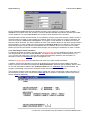
Selecting 'data set' 'Add' from the pull down menu and 'Calibration' from the 'create new data set' dialog
window displays the 'calibration data info window'.
The user has to provide the following information:
A. A descriptive name of the data set and the data set's directory name where the files needed for the
groundwater model calculations are located.
B. The name of the data sets the calibration set is based on; e.g. an 'Initial data set' and a 'Grid data set'.
Confirming the selection with the
-button causes the program to open the 'Calibration data set
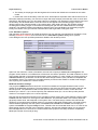
window', displaying all model parameters defined. The 'Calibration data set window' consists of three tabsheets:
Inherited parameters
Modified parameters
Result parameters
This sheet displays all model parameters defined in the (initial) data
set the calibration set is based on
This sheet displays all parameters created or modified in the (actual)
calibration data set
This sheet displays all parameters that result from the model
calculations. It is displayed only after model calculations have been
carried out.
5 Execution of Groundwater Flow Simulations: FLAIRS and MODFLOW-3
Royal Haskoning
Triwaco User's Manual
Double clicking on one of the parameters starts the graphical editor DigEdit. For each of the parameters the
user can create a new map and par file or modify the existing map and par file. These changes take place
in the directory of the Initial data set the Calibration set is based on!
Pressing the right hand mouse button displays the parameter pop-up menu. This menu allows the user to
retrieve 'Info', to 'View' or edit the map or par file, to 'View' the Ado file (the file containing the parameter
values assigned to the nodes of the grid), to 'Allocate' the parameter selected or to 'Modify' the parameter.
Choosing the Parameter pull down menu from the menu bar displays a slightly different selection of
possibilities: 'Info', 'Delete', 'Add', 'Allocate', 'View' ('Map', 'Par', 'Adore' and 'Adore as text'), 'Copy' and 'Paste'.
Selecting 'Modify parameter' moves the selected parameters from the 'Inherited parameters' Tab-sheet to
the 'Modified parameters' Tab-sheet. The parameter's original par and map files (in the Initial data set's
directory) remain unaffected and a new set of par and map files may be created. These files will be located in
the Calibration data set's directory.
To add or delete a parameter the 'Modified parameters' Tab-sheet should be active (visible). Only here a
parameter (other than the Inherited parameters) can be added. Adding a parameter displays the 'parameter
info window '. This window can also be accessed from the 'Info' command in the pull down and pop-up
windows. Deleting a (modified) parameter from the 'Modified parameters' Tab-sheet restores the original
settings for this parameter. The parameter reappears in the 'Inherited parameters' Tab-sheet.
5.1.3 Allocating model parameters
Selecting 'Allocate' from the parameter pull down or pop-up menu starts the selected allocator and an Ado or
Adore file will be generated. After allocation the status of the parameter will change from
to .
The Ado file contains an array with parameter values, interpolated at the locations of the nodes of the grid.
This array is preceded by the name of the parameter, a code indicating whether the array contains one
(constant) value or as many values as there are nodes and the number and format of values that follow. The
array is concluded with the text ENDSET. Such an array with parameter values is called an Adore set. The
number of values in the array depends on the type of parameter and equals the total number of nodes, the
number of river nodes, the number of source nodes or the number of boundary nodes. (see appendix B for a
complete overview and the lay out of the map, parameter and corresponding ado files, appendix C gives an
overview of currently available allocator types).
5 Execution of Groundwater Flow Simulations: FLAIRS and MODFLOW-4
Royal Haskoning
Triwaco User's Manual
5.1.4 Viewing the allocated parameters
Selecting ‘View Ado file’ from the parameter pull down or pop-up menu starts the graphical presentation
program TriPlot, loads the grid information and a spatially visualisation of the selected parameter. In this GIS
like environment the parameters can easily be checked, compared with other parameters on a spatial scale but
also for individual cells/nodes.
5.1.5 Definition of initial head parameters
The initial head for each aquifer is defined by HHi. The initial head for the topsystem is defined by HT.
Defining the initial head may be required for some cases. It is, however, more often used to speed up the
simulation run of Flairs in the calibration process or as initial heads for scenario calculations. The initial head
is then defined by the output of the former simulation result.
Triwaco computes groundwater heads/flow by iteration, starting from groundwater heads equal to 0.0. A
quicker calculation process may be obtained if initial headvalues are used which are closer to the heads to be
calculated. The initial head is often defined by the output of the former simulation result.
The initial head for each aquifer is defined by HHi. The initial head for the topsystem is defined by HT. These
parameters can be defined under the Modified-tab by choosing Parameter | Add | Internal. The
groundwaterhead from a former simulation result is defined by using an expression: PHIi (where i is the aquifer
number, HT is defined as PHIT).
5.1.6 Definition of a calibration file (calib.chi)
If a calibration file (calib.chi) is present, Triwaco automatically compares calculated hydraulic heads, fluxes
with the data from observation wells. After comparison Triwaco will calculate the average deviation, the
average absolute deviation, the squared average deviation, the minimum deviation and the maximum
deviation. To view or edit the calibration file select 'Calibration'|'Calibration'|'View/Create Input' from the pull
down menu. The input file has a fixed format described in chapter 10. The output of the calibration can be
viewed as table ('Calibration'|'Calibration'|'View Output') or as a background map in Triplot ('Calibration'
|'Calibration'|View Map'). A comprehensive description on the usage of the calibration (calib.chi) file is given in
chapter 10.
5 Execution of Groundwater Flow Simulations: FLAIRS and MODFLOW-5
Royal Haskoning
Triwaco User's Manual
5.2 Executing model simulations with FLAIRS
5.2.1 Introduction
Triwaco can handle two types of grids, Finite Element Grids and Finite Difference Grids. Once one of these
is selected in the ‘Grid definition’- window Triwaco will use the corresponding simulation package. The
choice between the two is depending on the type of problem, possibilities and/or limitations of the simulation
package. The default grid has finite elements with the corresponding simulation package Flairs. Flairs is a
three-dimensional saturated groundwater flow simulation program. The program uses triangular elements
with linear shape functions. The numerical calculations are based on Galerkin's method.
For Finite Difference Grid Triwaco uses ModFlow-96 provided by the USGS. ModFlow also is a threedimensional saturated groundwater flow simulation program. Executing model calculations with ModFlow is
explained in chapter 5.4.
5.2.2 Simulation Package FLAIRS
Flairs uses a Finite Element grid created by the program Tesnet and parameter files in Adore format
(generated by various allocators and with the extension *.ado). With the aid of the program TriPlot or other
Windows programs the results can be visualized as contour maps or hydrographs. The results can directly
be used for post-processing and auxiliary programs.
Flairs calculates the groundwater heads and fluxes in a groundwater domain that is divided into aquifers and
aquitards. Important features in Flairs are the rivers (line-source/sinks) and (point)-sources, which are
active within aquifers, and the large selection of different top systems that control the flux from the surface
or confining layer to the first aquifer. Hydrogeological parameters are given at the nodes of a Finite Element
Grid. These input parameters have to be available in Adore format.
The program is capable of handling a variety of problems, such as:
 steady-state and transient flow;
 anisotropy and inhomogeneities (Kxx, Kxy, Kyx, Kyy, Kzz);
 Dirichlet, Neuman and mixed boundary conditions;
 phreatic conditions possible for parts of the model area;
 multi-layered systems containing many aquifers and aquitards;
 flow in a vertical cross section;
 transient recharge imported from Fluzo, the Triwaco program for the calculation of flow in the
unsaturated zone;
 (non)linear recharge relations for sources and sinks, rivers, boundaries and top-systems,
 groundwater flow under variable density conditions,
 clustering of rivers (line-sinks) or sources to simulate drains or multi-screen wells with given abstraction
rate.
The mathematical background of the simulation package is given in paragraph 5.3.
The program requires a number of readable (standard ASCII) input files and generates various output files.
When used in combination with the TriShell default file names are assumed for all input and output files.
5.2.3 Simulation options
After allocation of the values for all model parameters one may start the groundwater flow calculations. First,
selecting 'Calibration' 'Options' from the menu bar, the 'Calculation options' dialog box is opened.
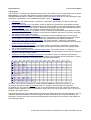
In this dialog box the user specifies parameters related to the iteration process:
Description
Inner iteration
Outer iteration
Function
Sets the maximum number of inner iterations
Sets the maximum number of outer iterations
Convergence
Sets the criterion for convergence
Relaxation
Sets the relaxation factor
5 Execution of Groundwater Flow Simulations: FLAIRS and MODFLOW-6
Royal Haskoning
Triwaco User's Manual
During calculations Flairs will pause and display a warning if the maximum number of linear or inner
iterations is exceeded. If the user decides to continue calculations Flairs automatically doubles the number
of inner iterations. For each outer iteration, the number of inner iterations will be checked.
Calculations will proceed until the number of inner iterations during a single outer iteration equals 2 or less or
until the maximum number of outer iterations is reached. Apart from the maximum number of iterations, the
user has to specify a criterion for convergence. The program checks whether or not differences are less
than the criterion specified. The initial conditions for each outer iteration depend on the head change between
(outer) iterations. In case of badly converging systems a relaxation factor may be defined. In that case the
head change between (outer) iterations is multiplied with the relaxation factor. This causes a more stable
iteration process but also results in smaller head changes, thus requiring more iterations to reach a solution.
5.2.4 Executing the model simulation
For starting the model calculations one first selects 'Generate input' from the Calibration pull down menu bar.
This will generate the input file needed (flairs.fli). This input file may be viewed or edited selecting 'View'
'Input' from the pull down menu. The input file contains all parameters needed for the calculations. A
description of the input file flairs.fli is given in paragraph 5.2.6.
Selecting 'Run Simulation' from the Calibration pull down menu starts model simulations.
A window, showing the calculation process will be displayed and the program will be added to the tasks
window. Once the calculation has stopped the 'Result parameters' Tab-sheet will be updated. After the first
run this Tab-sheet will be added to the 'Calibration data set'. If a 'calibration file' has been defined, the
program automatically compares the calculation results with the observed heads/fluxes.
The simulation program produces different types of output files. Some of these files contain information on
the calculation process, errors encountered, (flairs.flg) others contain the calculation results using various
formats (flairs.flp, flairs.flo).
5 Execution of Groundwater Flow Simulations: FLAIRS and MODFLOW-7
Royal Haskoning
Triwaco User's Manual
Triwaco computes groundwater heads/flow by iteration, starting from groundwater heads equal to 0.0. A
quicker calculation process may be obtained if initial headvalues are used which are closer to the heads to be
calculated. The initial head is often defined by the output of the former simulation result. Definition of the initial
head is described in par. 5.1.5.
5.2.5 Viewing output results (maps)
Selecting 'View' 'Results' from the Calibration pull down menu starts the graphical presentation program
TriPlot, loads the grid information and displays the layout of the model area. Now the user can contour or
classify the result parameters and view the results in plane view or can select a cross-section of the model
area.
Alternatively, the user can select one of the parameters from the 'result parameters' sheet and viewing the
parameter separately selecting 'View' 'Adore' from the Parameter pull down menu or 'View Adore file' from
the pop-up menu (right hand mouse button). Adding other parameters (selecting 'Param' 'Load' from the
TriPlot menu bar) gives the user the opportunity to compare result parameters with model input parameters.
5.2.6 Input data description
The input file (flairs.fli) for the groundwater simulation program contains the definition of the hydrogeological
system, including references to all input parameter files, boundary conditions, output options and so on. The
input file may be generated automatically from the TriShell or edited manually.
The input required in the flairs.fli consists of the following sets:
Set 1:
HEAD
· identification of project or grid
Format A40
HEAD is an alphanumerical string for identification of the project's grid
Set 2:
Naq, Iffr, Ifss, Ifsf, Iftr, Nsar, Rrlax
Naq
Iffr
Ifss
·
·
·
·
·
·
·
number of aquifers
flag for confined / phreatic calculations
flag for steady-state / transient calculations
flag for variable density or salt / fresh water interface
dummy flag (used only in previous versions of Flairs)
number of sub-areas for water balance calculation
relaxation factor for non-linear iterations
Format
6(I5), F10.4
the number of aquifers
a flag for (semi) confined (=0) or phreatic (=1) calculations
a flag for steady state (=0) or transient (=1) computations; also used for the definition of the
Surface water option (FLAIRSSF).
5 Execution of Groundwater Flow Simulations: FLAIRS and MODFLOW-8
Royal Haskoning
Ifsf
Iftr
Nsar
Rrlax
Triwaco User's Manual
a flag for absence (=0), presence (=1) of a salt/fresh water interface, variable density
(FLAIRSVD)(=2)
a dummy-flag (in former versions for preparing Trace output)
the number of sub-areas a water balance will be calculated for
the relaxation factor for the non-linear iterations.
Set 3a:
NB
NB
· number of boundary points for water balance subareas
Format I5
the number of boundary points defining the sub-area for water balance calculations (NB
Set 3b:
XB, YB
· coordinates of boundary points for water balance subareas
20)
Format 2(F10.4)
XB,YB
the X and Y coordinates of the boundary points. The coordinates of the last boundary point are
not necessarily equal to the coordinates of the first boundary point.
Set 3b will be repeated (NBP-1) times.
Sets 3a and 3b should be repeated Nsar times, for each of the water balance sub-areas, and omitted if Nsar
= 0.
Set 4a:
HCU, NCriv, NCsrc
HCU
NCriv
NCsrc
· name of collection unit
· number of rivers in collection unit
· number of sources in collection unit
identification string for the collection unit. A collection unit is a combination of rivers and
sources for which the total recharge is computed and written tot the print output file flairs.flp
number of rivers belonging to the collection unit
number of sources belonging to the collection unit
Set 4b:
ICriv, Iaq, Iriv
Format
A20, 2(I5)
· sequential number of collection unit's river
· aquifer number of river
· river number / river ID
Format 3(I5)
ICriv
sequential number of the river, ICriv = (1,,NCriv)
Iaq
sequential number of the aquifer the river or source is active in
Iriv
identification number of the river involved
Set 4b will be repeated NCriv times.
Set 4c:
ICsrc, Iaq, Isrc
· sequential number of collection unit's source
· aquifer number of source
· source number / source ID
Format 3(I5)
ICsrc
sequential number of the source, ICriv = (1,,NCsrc)
Iaq
sequential number of the aquifer the river or source is active in
Isrc
identification number of the source involved
Set 4c will be repeated NCsrc times.
Set 4
should be repeated for each collection unit and omitted if no collection units are defined. The
maximum number of collection units equals 50.
Set 5:
End of sum input
· literal text string
This string should always be present, it indicates the end of the section
5 Execution of Groundwater Flow Simulations: FLAIRS and MODFLOW-9
Royal Haskoning
Triwaco User's Manual
Set 6:
Isrc, Iaq, Ist, Qsrc, Hsrc
Isrc
Iaq
Ist
If Ist =0
If Ist =1
Qsrc
Hsrc
·
·
·
·
·
source ID
active aquifer number
type of source
discharge or recharge rate
groundwater head
Format
3(I5), 2(E10.4)
the source ID as defined in the grid.teo file
the number of the aquifer the source is active in
a flag for identifying the type of sources
the source is defined by a given rate Qsrc
the source is defined by a given head Hsrc
abstraction or infiltration rate (Qsrc<0: abstraction)
fixed groundwater head
Set 6 should be repeated as many times as required.
In stead of using Set 6, sources are generally defined using the source parameter sets ISi, SHi and SQi
(i=1,,N). Moreover, using the source parameters, the user may also specify 'clustered' sources (ISi=2).
The use of source parameter sets overrides the values defined by Set 6.
If no source parameter sets are defined, sources that are not defined by Set 6 will have a default abstraction
rate of Qsrc=0 (with source type Ist=0).
Set 7:
End of sources input
· literal text string
This string should always be present, it indicates the end of the section
Set 8:
Ibnd, Iaq, Ibt, Hbnd
Ibnd
Iaq
Ibt
. If Ibt =0
. If Ibt =1
Hbnd
·
·
·
·
boundary point number
active aquifer number
type of boundary
groundwater head
the boundary point number as defined in the grid.teo file
the number of the aquifer the boundary condition is given for
a flag for identifying the type of boundary condition
the boundary is defined by a given head Hsrc
the boundary is defined by a head dependent flux
fixed groundwater head (for Ist =0)
or
Ibnd, Iaq, Ibt, BA, BB
BA, BB
Format
3(I5), E10.4
·
·
·
·
·
boundary point number
active aquifer number
type of boundary
head dependent flux parameter
head dependent flux parameter
Format
3(I5), 2(E10.4)
head dependent flux parameters (for Ist =1)
Set 8 should be repeated as many times as required.
In stead of using Set 8, boundary conditions are generally defined using the boundary parameter sets IBi,
BHi, BAi and BBi (i=1,,N). Parameters BAi and BBi define the head dependent boundary flux (IBi=1).
The use of boundary parameter sets overrides the values defined by Set 8. If no boundary parameter sets
are defined, boundaries that are not defined by Set 8 will have a default boundary head of Hbnd=0 (with
boundary type Ibt=0).
Set 9:
End of boundary input
· literal text string
This string should always be present, it indicates the end of the section
5 Execution of Groundwater Flow Simulations: FLAIRS and MODFLOW-10
Royal Haskoning
Triwaco User's Manual
Set 10:
Iriv, Iaq, Irt, Hriv
Iriv
Iaq
Irt
. If Irt =0
. If Irt =1
Hriv
·
·
·
·
river ID
active aquifer number
type of river
river water level
the river ID as defined in the grid.teo file
the number of the aquifer the river is active in
a flag for identifying the type of boundary condition
the river is defined by a given water level Hriv
the river is defined by a given flux Qriv
the river water level (for Irt =0)
or
Iriv, Iaq, Irt, Qriv, Nclus
Qriv
Nclus
Format
3(I5), E10.4
·
·
·
·
·
river ID
active aquifer number
type of river
river discharge or recharge
river cluster number
Format
3(I5),
E10.4, I5
the recharge or discharge rate (for Irt =1)
the river cluster number (for Irt =1); clustered rivers will have the same head.
Set 10 should be repeated as many times as required.
In stead of using Set 10, the rivers are generally defined using the river parameter sets RAi, HRi, and RQi
(i=1,,N). The value for RAi equals (Irt+1). For clustered rivers the parameter RCi should be defined also.
The use of river parameter sets overrides the values defined by Set 10. If no river parameter sets are
defined, rivers that are not defined by Set 10 will not be active (equivalent to RAi=0).
Set 11:
End of river input
· literal text string
This string should always be present, it indicates the end of the section
In stead of using Sets 6, 8 and 10 the user is advised to define the parameters in question by the appropriate
parameter sets (Adore -files). The text strings defined in Sets 7, 9 and 11, however, should never be
omitted.
In the next section all model parameters are being defined. The boundary, river and source parameters
mentioned above should be defined here too, unless the user has specified Sets 6, 8 and 10.
Set 12: consists of three records
Pname
Fname
FPname
Pname
Fname
FPname
· Triwaco parameter name
· parameter file name
· user defined parameter name
Format A4
Format A60
Format A20
is the pre-defined Triwaco parameter name
the name of the file containing the parameter, including the full path
a user defined name describing the parameter; this name may be different from the predefined
parameter name.
Set 12 should be repeated as many times as required. If Pname is not one of the pre-defined Triwaco
parameter names, Set 12 will be ignored. Parameters that are not defined by Set 12 will obtain a default
value equal to 0, except for the anisotropy parameters PYi and TYi, which will be assigned the value of the
corresponding PXi and TXi.
Set 13:
End
· literal text string
This string should always be present, it indicates the end of the section
5 Execution of Groundwater Flow Simulations: FLAIRS and MODFLOW-11
Royal Haskoning
Triwaco User's Manual
In the next section the calculation parameters are being defined. One can discriminate between parameters
needed for steady-state calculations and those needed for the transient calculations only. Of course the latter
only need to be present if transient calculations are required and Ifss=1 (see Set 2).
Set 14:
IImax, IOmax, EPS
IImax
IOmax
EPS
· maximum number Inner Iterations
· maximum number Outer Iterations
· convergence criterion
Format 2(I5), E10.4
the maximum number of iterations allowed for the linearized equations
the maximum number of iterations allowed for the non-linear equations
the criterion for convergence for the linearized equations
For steady-state calculations continue with Set 17.
Set 15a:
Ngrf
Ngrf
· number of nodes for time series
the number of nodes for which time-series output will be generated
Set 15b:
I1, I2, …, INgrf
Ii
Format I5
· node number for time series
Format 16(I5)
(i=1,,Ngrf) the numbers of the FE-nodes for which time-series output is required. The node
numbers correspond with the numbers from the FE-grid file grid.teo
Set 15b should be repeated Ngrf/16 times and omitted if Ngrf=0.
The time-series output for the Ngrf nodes defined by the node numbers of Set 15b are written to the output
file graphnode.out.
Set 16:
Tend, DHmx, DT
Tend
DHmx
DT
· stress input time
· maximum allowable head change per time
step
· initial time-step size
Format 3(E10.4)
the stress-input time or time at which a new time-step starts and new input data may be
defined (end time of calculation period)
the maximum allowable change in groundwater head per time-step for the time period
considered
the size of the initial time-step for the time period considered
Set 17:
Iprn, Irst, Iphit, Iqrch,
(Iphin, Iqkwn)n=1,,Naq
(Iqrin, Iqscn)n=1,,Naq
Iprn
. If Iprn=0
. If Iprn=1
. If Iprn=2
Irst
. If Irst=0
. If Irst=1
Iphit
Iqrch
· print and output flags
Format (4+4n)I5
code for printing (=1) or not printing (=0) calculation results to the print output file flairs.flp
(default value 0, no print output)
calculation results not to the print output file
calculation results to the print output file (default)
calculation results to the print output file and top-system fluxes will be written to file Top4Q.out
(only if top-system 4 is selected) and flairs.flo
code for generating restart record
no restart record (default)
a restart record will be written at time TEND (transient calculations only)
code for writing (=1) or not writing (=0) calculation results for the parameter PHIT to the output
files flairs.flo (default value 1)
code for writing (=1) or not writing (=0) calculation results for the parameter QRCH to the
output files flairs.flo (default value 1)
5 Execution of Groundwater Flow Simulations: FLAIRS and MODFLOW-12
Royal Haskoning
Iphin
Iqkwn
Iqrin
Iqscn
Triwaco User's Manual
code for writing (=1) or not writing (=0) calculation results for the parameter PHIn (n ranges
from 1 to Naq, see Set 2) to the output files flairs.flo (default value 1)
code for writing (=1) or not writing (=0) calculation results for the parameter QKWn (n ranges
from 1 to Naq, see Set 2) to the output files flairs.flo (default value 1)
code for writing (=1) or not writing (=0) calculation results for the parameter QRIn (n ranges
from 1 to Naq, see Set 2) to the output files flairs.flo (default value 1)
code for writing (=1) or not writing (=0) calculation results for the parameter QSCn and QBOn
(n ranges from 1 to Naq, see Set 2) to the output files flairs.flo (default value 1)
The flags Iphit, Iqrch and following are only required in case of transient calculations. Selecting a value 0 (not
writing to output) diminishes the size of the output file considerably. However, calculation results for those
parameters will be lost. Note that the last flag for QKWn (n=Naq) is a dummy, because the parameter does
not exist.
Set 17 is the last input set for steady state calculations.
For transient calculations a number of input sets have to be repeated to define new input at successive
stress-input times or to redefine the calculation parameters and print output options if desired.
Set 18 to 25 redefine the input parameters by repeating Sets 6 to 13.
Starting at stress-input time TEND (the end of the previous calculation period, see Set 16) new parameter
values may be defined. If a parameter is not redefined the values from the previous calculation period are
assumed to remain valid.
At least the Sets 7, 9, 11 and 13 should be repeated.
Set 26 and 27 are similar to Set 16 and 17 and redefine the transient calculation parameters and the print
output options. A new stress-input time TEND will be defined, and new values for the initial time-step or
maximum allowable head change may be given.
Sets 18 to 27 should be repeated for every new stress-input time, thus producing Sets 28+n *10 to 37+n *10.
The transient calculation stops if the value of TEND, defined in one of the Sets 26 or 36+n *10, is smaller than
the previous value of the parameter Tend.
Example Flairs input file Flairs.fli
Set
1
2
3a
3b
3b
3b
3b
3b
3a
3b
3b
3b
3b
5
7
9
11
12
12
12
12
Example text
MATRIX Transient calculation
3 1 1 0 0 2 1.0000
5
142811
471333
142654
471117
142890.11 470345.87
143169
470972
142884
471332
4
142338.13 470137.27
142968.77 470229.18
142578.13 470333.86
142324.09 470356.84
end of sum input
end of sources input
end of boundary input
end of river input
IR
..\Calib\IR.ado
IR
RP2
..\Calib\RP2.ado
RP2
RP3
..\Calib\RP3.ado
RP3
……
HT
HT.ado
HT
5 Execution of Groundwater Flow Simulations: FLAIRS and MODFLOW-13
Royal Haskoning
Triwaco User's Manual
12
HH1
HH1.ado
HH1
12
SC1
SC1.ado
Storage Coeff Aqf 1
……
12
RP1
RP1.ado
RP1,TIME= 0.00
13
end
15a
100 100.00001000
15b
0
16
10.0000 1.0000 0.2500
17
1 0 1 1 1 1 1 1
7
end of sources input
9
end of boundary input
11
end of river input
12
RP1
RP1.ado
RP1,TIME= 10.00
13
end
16
20.0000 1.0000 0.2500
17
1 0 1 1 1 1 1 1
7
end of sources input
9
end of boundary input
11
end of river input
12
RP1
RP1.ado
RP1,TIME= 152.00
13
end
16
162.0000 1.0000 0.2500
17
1 0 1 1 1 1 1 1
7
end of sources input
9
end of boundary input
11
end of river input
12
RP1
RP1.ado
RP1,TIME= 345.00
13
end
16
345.0000 1.0000 0.2500
17
1 0 1 1 1 1 1 1
7
end of sources input
9
end of boundary input
11
end of river input
13
end
16
0.0000 1.0000 0.2500
File ends with an empty line
END OF FILE
1
1
1
1
1
1
1
1
1
1
1
1
1
1
1
1
1
1
1
1
1
1
1
1
1
1
1
1
1
1
1
1
5.2.7 Output data description
The simulation program produces different types of output files. Some of these files contain information on
the calculation process (flairs.flg) others contain the calculation results using various formats (flairs.flp,
flairs.flo), and the time-series output file graphnode.out).
Print output file (flairs.flp)
Selecting 'View' 'Print' from the Calibration pull down menu displays the print output file (flairs.flp). This file
contains information on the water balances of the various aquifers, including the error in the water balance for
each aquifer. These errors should be within reasonable limits, e.g. less than a few percent at a maximum.
Furthermore, the discharges towards the rivers, sources and boundaries are summarized.
The print output file flairs.flp is always generated and contains:





A water balance for every aquifer. For transient calculations this water balance is given for every time
step together with a cumulative water balance.
A water balance for the sub-areas defined in the input file (usage described together with flairs.fli).
The total recharge or discharge for each collection unit defined in the input.
The recharge from or the discharge towards all river nodes.
The recharge from or the discharge towards all point sources and sinks.
5 Execution of Groundwater Flow Simulations: FLAIRS and MODFLOW-14
Royal Haskoning

Triwaco User's Manual
The boundary heads and boundary fluxes for all boundary nodes.
Optionally the following output may be added to the print file, provided the corresponding print-flags are
enabled in the flairs.fli-input file:



The groundwater heads for each aquifer and for every node.
The location of the salt-fresh water interface for every node.
The recharge from the top-system and the leakage through the aquitards for every node.
In case of transient calculations this output is given at the end of every calculation period for which the user
enabled print output by setting the appropriate flag. If all print-flags are enabled the print file may become
very large. Therefore, by default these print-flags are disabled and the print file only contains the water
balances and an overview of the river, source and boundary fluxes.
Simulation log file (flairs.flg)
Selecting 'View' 'Log' displays the execution log file (flairs.flg). This file contains information on the progress
of the calculation process. Any error during the simulation are written to this file. The following information is
written to this file:



General information regarding the used grid, the number of aquifers, the type of the top aquifer and the
computation of a salt-fresh water interface.
Information concerning the input parameters and the parameter files used. Warnings and Error
messages are included.
Information concerning the iteration process. The convergence criterion, the maximum number of
iterations and the number of iterations used are reported.
Consultation of the execution-log file is advised whenever an error message is generated. Even if the
calculation seems to have finished without problems, a quick check of the log file may confirm whether or not
the program has terminated correctly.
Simulation result file (flairs.flo)
Finally, all calculation results are stored in the result file flairs.flo, which contains the output parameters in
Adore format. These parameters provide the result of the calculation.
For steady-state calculations the output file contains the following variables:









average groundwater heads for the top-system,
groundwater heads for each aquifer,
piezometric head at the salt-fresh water interface,
recharge to the top-system,
(sum of drainage/infiltration in topsystem)
leakage through the separating layers,
discharge or recharge of rivers for each aquifer,
discharge or recharge of sources for each aquifer,
boundary fluxes for each aquifer.
Similarly, for transient calculations the output file contains the following variables:







average groundwater heads for the top-system at the end of each period,
groundwater heads for each aquifer at the end of each period,
recharge to the top-system at the end of each period,
leakage through the separating layers at the end of each period,
discharge of rivers for each aquifer at the end of each period,
discharge of sources for each aquifer at the end of each period,
boundary fluxes for each aquifer at the end of each period.
5 Execution of Groundwater Flow Simulations: FLAIRS and MODFLOW-15
Royal Haskoning
Triwaco User's Manual
The parameter sets in the file flairs.flo have the following names:
steady-state calculations
Phreatic and piezometric heads
PHIT, STEADY-STATE==
PHIx, STEADY-STATE==
(x = number of aquifer)
Variable density correction fluxes
V10nn, STEADY-STATE==
V20nn, STEADY-STATE==
V30nn, STEADY-STATE==
Top system fluxes and leakage
QSxx, STEADY-STATE==
QRCH, STEADY-STATE==
transient calculations
PHIT,TIME:nnnnnnnnnn
PHIx,TIME:nnnnnnnnnn
V10nn, STEADY-STATE==
V20nn, STEADY-STATE==
V30nn, STEADY-STATE==
(QDR1, STEADY-STATE==)
QKWx, STEADY-STATE==
(x indicates leakage from aquifer x + 1 to aquifer x)
Recharge and discharge to rivers
QRIx, STEADY-STATE==
Recharge and discharge to sources
QSCx, STEADY-STATE==
Boundary fluxes
QBOx, STEADY-STATE==
(x = number of aquifer)
QSxx,TIME:nnnnnnnnnn
QRCH,TIME:nnnnnnnnnn
( QDR1, TIME:nnnnnnnnnn)
QKW x,TIME:nnnnnnnnnn
QRIx,TIME:nnnnnnnnnn
QSCx,TIME:nnnnnnnnnn
QSCx,TIME:nnnnnnnnnn
The string ‘nnnnnnnnnn’ stands for one of the output times defined by the user; the format used for the
output times is (F10.4). The length of the output parameter name is in all cases twenty characters, including
spaces or blanks.
Drainage result file (top4q.out)
If applicable for topsystem 4 (see input description) then the drainage/infiltration fluxes are written to
top4q.out. Is same as Qsxx,.. in the flairs.flo file.
steady-state calculations
Drainage /infiltration fluxes
TOP1 AT TIMESTEP 1
TOP2 AT TIMESTEP 1
TOP3 AT TIMESTEP 1
TOP4 AT TIMESTEP 1
transient calculations
TOP1 AT
TOP2 AT
TOP3 AT
TOP4 AT
TIMESTEP nnn
TIMESTEP nnn
TIMESTEP nnn
TIMESTEP nnn
Where the result of :
• TOP1 is governed by the topsystem parameters RP4 (drainage resistance),RP7 (infiltration resistance)
and RP10 (base elevation of system)
• TOP2 is governed by the topsystem parameters RP5 (drainage resistance),RP8 (infiltration resistance)
and RP11 (base elevation of system)
• TOP3 is governed by the topsystem parameters RP6 (drainage resistance),RP9 (infiltration resistance)
and RP12 (base elevation of system)
• TOP4 is governed by the topsystem parameters RP13 (surface level)
Graphnode (graphnode.out)
The output file graphnode.out contains time-series output for transient calculations. For a number of nodes,
defined by the user in the input file for transient calculations, groundwater heads and the interface can be
written as a function of time. The time and parameter values are exported to the time-series output file
(graphnode.out). The time-series data is listed in columns. The first of these columns contains the time
value, the other columns contain values for the various parameters, successively for each of the grid nodes
specified. The heading of the file specifies for which nodes parameters have been exported to the time-series
output file. The information from the time-series output file can easily be imported in a spreadsheet.
5 Execution of Groundwater Flow Simulations: FLAIRS and MODFLOW-16
Royal Haskoning
Triwaco User's Manual
5.2.8 Command line calls
Program for the calculation of groundwater flow; program name: Flawin95, FlawinVD, FlawinVDEXT.
Normally if a calibration file (calib.chi) exists a comparison between calculated and observed heads will be
carried out.
A standard input file (flairs.fli) must be generated from the TriShell. Also, a standard grid file (grid.teo) is
required. Output will be written to files: flairs.flo, flairs.flp and flairs.log. If no arguments are given the
program opens in Windows mode. The appropriate input files (grid.teo, flairs.fli and calib.chi ) can be
selected and the program may be run using the pull-down menus.
Command line call:
Flawin95.exe [set-dir grid-dir flairs.fli calib.chi [options]]
One may choose from the following options:
-c
-f
no calibration file checking
no Flairs computation
Example:
Flawin95 C:\model\cal C:\model\grid flairs.fli calib.chi
Flawin95 C:\model\cal C:\model\grid flairs.fli calib.chi -f
5 Execution of Groundwater Flow Simulations: FLAIRS and MODFLOW-17
Royal Haskoning
Triwaco User's Manual
5.3 Mathematical background of FLAIRS
5.3.1 Introduction
In this documentation, a description will be given of the governing differential equations and the Finite
Element formulation of these equations. Furthermore a description will be given of the way recharges and
fluxes are treated in the program. Special options, such as anisotropy and phreatic transmissivity are
discussed and the way the Finite Element equations are solved will be described.
5.3.2 Partial differential equation
The partial differential equation that is solved (by approximation) in the program Flairs, follows from Darcy's
law and the equation of continuity. In the derivation of the equations the Dupuit-Forchheimer assumption is
used, so that the partial differential equation can be written in terms of the potential 'h' (or groundwater head)
as:
[1]
There are no restrictions on the transmissivity tensor 'T '. Therefore, the transmissivity can be anisotropic,
while the principal directions do not coincide with the coordinate axes.
For a multi-aquifer system, the equation [1] holds for each aquifer. The aquifers are coupled through the
recharge term 'q'.
The top aquifer may be phreatic. In that case, transmissivity is a function of the groundwater head and the
permeability of the aquifer, while storativity changes if the aquifer changes from confined to phreatic
conditions.
In the lower most aquifer a salt-fresh water interface may be present. The salt water is assumed to be at rest,
and the interface can be obtained from the 'Badon-Ghijben / Herzberg' equation. In that case, transmissivity
is again a function of the groundwater head and the aquifer permeability. Also storativity changes when the
aquifer changes from completely fresh to partly fresh. (Note that Flairs should not be used for transient
calculations with a salt fresh water interface, due to the assumption of a stagnant salt-water body). Phreatic
conditions and a salt-fresh water interface may be defined in one and the same aquifer in case of single
aquifer systems.
In case of transient calculations, or if salt water is present in more than one aquifer the variable density
module of FLAIRS (FLAIRSVD) should be used. The use of this module requires additional input and some
minor changes in the standard Flairs input file which is carried out in the TriShell automatically when the
corresponding Program Group is choosen in the Grid data set.
5 Execution of Groundwater Flow Simulations: FLAIRS and MODFLOW-18
Royal Haskoning
Triwaco User's Manual
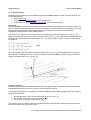
The recharge term 'q' comprises a number of different effects. In the program Flairs, 'q' is divided into four
distinctive components, depending on the origin of the water:
recharge from a top-system at the top of the uppermost aquifer due to e.g. precipitation, infiltration etc.;
- leakage through the separating aquitards between aquifers;
- discharge to point sources or recharge from point sinks;
- discharge to rivers and drains and recharge from line-sinks.
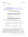
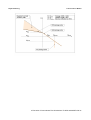
A multi-aquifer system with several recharge terms is shown below. Note, that the numbering of aquifers and
aquitards in Triwaco is always top down, and the number of aquifers is one greater than the number of
aquitards. The layer covering the uppermost aquifer is also referred to as aquifer number 0, and is part of the
top-system.
5.3.3 Finite element equations
The Finite Element equations are derived from the partial differential equation given in equation [1].
Subdividing the recharge term 'q' in four distinctive components, this equation is written as:
[2]
The components of the recharge term are:
Recharge from the top-system (the shallow drainage system)
Recharge due to leakage
Recharge from rivers, canals and drains
Recharge from sources or sinks
For the sake of simplicity the first four terms of the equation [2] will be combined:
[3]
with 'T ' representing the transmissivity tensor.
The Finite Element equations are derived using Galerkin's method. The following simplifying assumptions
are made:

The spatially distributed recharge terms '
' (recharge) and '
' (leakage) can be approximated by
an infiltration or abstraction in the nodal points of the grid. If the value '
the strength at that point is given by:
' in point 'i' is given by '
',
[4]
where '
' represents the area of influence of nodal point 'i'.

The recharge due to rivers, canals and drains can be approximated by a series of point sources or
sinks situated in a series of nodal points (the river nodes).

The transmissivities and storage coefficients are constant within an element and are equal to the
average of the values at the nodal points.
This so-called lumped parameter approach has the advantage that these terms are easily incorporated and
the system of equations will be symmetric.
We will now define an 'a priori' solution for the given differential equation:
5 Execution of Groundwater Flow Simulations: FLAIRS and MODFLOW-19
Royal Haskoning
Triwaco User's Manual
[5]
with:
the unknown coefficient
a known shape function
The shape functions are defined piecewise linear, such that:
Hence, '
= 1,
in nodal point 'i'
= 0,
in all other nodal points.
' will have the value of '
Substitution of '
' in nodal point 'i'.
' in the partial differential equation results in the following equation:
[6]
The coefficients '
' have to be determined such, that 'R' is minimized over the model area. The value of 'R'
is minimized by making it orthogonal with the shape functions '
':
[7]
and integrating over the model area 'G'.
The integration can be performed by using Greens theorem:
[8]
with:
n
the boundary of the model area
the normal on the boundary directed outward.
Using Darcy's law one obtains:
[9]
with:
the flux across the boundary into the model area.
5 Execution of Groundwater Flow Simulations: FLAIRS and MODFLOW-20
Royal Haskoning
Triwaco User's Manual
Through substitution of the approximate solution and approximation of the boundary flux by a series of point
sources or sinks, we obtain the following Finite Element equation:
[10]
The time derivative has been given by a completely implicit finite difference equation. The integrations in the
equations can be easily performed, due to the simple form of the shape function.
Note that, due to the definition of the different recharge terms, the Finite Element equations can be nonlinear.
This implies that both nonlinear and linear iterations have to be carried out to solve the equations.
The linear iterations, used to determine the solution of a linearized system of equations, are referred to as
inner iterations.
The nonlinear iterations are referred to as outer iterations. These are used to update the linearization of the
equations in order to obtain an accurate solution to the nonlinear problem.
5.3.4 Solution technique
The resulting Finite Element equations will generally form a system of nonlinear equations, mainly due to the
nonlinear character of the recharge term 'q'. Moreover, the fact that both the transmissivity and the storativity
of the top or bottom aquifer may change with the groundwater head, also results in non-linearity of the
equations. This is the case whenever phreatic conditions or a salt-fresh water interface are present.
The Finite Element equations are given in an implicit way. So, they contain parameters related to the
(unknown) groundwater head at the new time level; for instance the recharge 'q'. Hence, the recharge 'q' will
be unknown too.
The recharge 'q' is approximated in the following way:
[11]
In case of phreatic conditions both the transmissivity and the storativity are calculated for the known values of
the groundwater head. The resulting linear equations are solved by the conjugate gradient method. When
a solution is found, the process may be repeated using the new values of the groundwater head.
Thus, two types of iterations are performed:
● inner iterations or linear iterations;
● outer iterations or nonlinear iterations.
For both types of iterations, the user defines the maximum number of iterations allowed. A maximum for the
number of linear or inner iterations is, as a rule of thumb, equal to the total number of unknowns, which will
be sufficient in most cases. The number of outer iterations required is strongly dependent on the non-linearity
of the different terms. For a completely linear system, one single outer iteration is sufficient. The number of
iterations for more complex situations may increase strongly with complexity. Default the program sets the
maximum number of outer iterations to 100, a number that is hardly ever reached, and the maximum number
of inner iterations to 500. If the number of inner iterations appears not to be sufficient, the program asks the
user whether or not to continue the calculations. If the user agrees to continue the program doubles the
number of inner iterations allowed.
5 Execution of Groundwater Flow Simulations: FLAIRS and MODFLOW-21
Royal Haskoning
Triwaco User's Manual
The program will stop if the maximum number of outer iterations is exceeded. For each outer iteration, the
number of inner iterations will be checked. For transient calculations the program will proceed with a new
time step if the maximum number of outer iterations has been reached, or if the number of inner iterations
during an outer iteration equals 2 or less.
Apart from the maximum number of inner iterations, the user has to specify a criterion for convergence ' '.
The program checks whether or not the norm of the right-hand side vector and the residual vector differ less
than the criterion given.
Hence, if the system of equations to be solved is given in matrix notation:
[12]
the residual vector becomes, for an approximate solution:
[13]
and we accept '
' as the correct solution if
[14]
where:
[15]
For a description of the conjugate gradient method, the user is referred to the handbooks on numerical
methods.
When transient calculations are carried out, the user also has to provide the maximum change in
groundwater head that is allowed during each time step. The program will now compute the size of the time
step to be used. This time step depends on the maximum change in groundwater head during the previous
time step and the maximum allowable change defined by the user. If the calculated change 'dh' is smaller
than the allowable change '
', the new time step will become:
[16]
If the change in groundwater head ('dh') during a time step is greater than the maximum change '
calculation will be repeated once with a time step:
', the
[17]
Hence, the multiplication factor between two successive time-steps varies between a minimum value of 0.5
and a maximum of 2.0.
5 Execution of Groundwater Flow Simulations: FLAIRS and MODFLOW-22
Royal Haskoning
Triwaco User's Manual
5.3.5 Recharge terms and Boundary fluxes
As discussed in the previous section, vertical recharge into an aquifer can be divided into four parts,
depending on the origin of the water (see equation [2]):




recharge from or discharge towards a so-called top-system;
recharge or discharge due to leakage through a separating layer;
recharge from or discharge towards rivers, canals and drains;
recharge from sinks or discharge towards sources.
Horizontal recharge is given by the boundary fluxes. In this section all recharge terms are treated in more
detail. In all cases a relation between the recharging (or discharging) flux and the piezometric head in the
aquifer can be defined. These relations vary from simple to very complicated as can be seen from the
description of the various recharge terms in the following sections. First the boundary fluxes are treated and
next the vertical recharge terms, in order of increasing complexity.
Boundary fluxes
Boundary fluxes can be considered to result from a line source or line sink in the two-dimensional model
area. In the Finite Element program, these line sources are approximated by a series of point sources located
at the boundary nodes. The boundary flux is defined positive flowing into the model area.
There are two ways in which the boundary fluxes can be calculated:

The groundwater head at the boundary may be given and the flux will be calculated as function of the
gradient of the groundwater head at the model's boundary.
[18]

The groundwater flux across the boundary is given as function of the groundwater head at the boundary.
[19]
Here 'Ba' (m3/d per m2 = m/d) and 'Bb' (m3/d per m1 = m2/d) are the boundary flux parameters.
A given (constant) flux, independent of the groundwater head, may be obtained by setting the value for 'Ba' to
zero. Setting the value for 'Bb' also to zero, a 'natural' or no-flow boundary is created.
Both types of boundary conditions can be used simultaneously for parts of the boundary. The type of
boundary condition that will be used is determined by the boundary type parameter, to be defined by the
user. By default the program assumes the boundary condition to be defined by a given head.
Leakage
The leakage term (' ' in the equations) defines the flow of groundwater between two adjacent aquifers. The
leakage is defined assuming the following simplifications:


The flow in the aquitards is vertical.
The storage in aquitards can be neglected.
Taking these two assumptions into account, the leakage term is given by the next equation:
[20]
with:
the groundwater head in the aquifer under consideration,
the groundwater head in the adjacent aquifer
the hydraulic resistance of the aquitard
5 Execution of Groundwater Flow Simulations: FLAIRS and MODFLOW-23
Royal Haskoning
Triwaco User's Manual
Sources
In the program Flairs the terms 'sources' and 'sinks' are reserved for groundwater abstractions or infiltrations
defined in nodal points. These nodal points have to be defined as such in the Finite Element Grid. The
abstraction or infiltration rate of a point source or sink can be defined in two ways in the program:

An abstraction or infiltration can be defined by a given rate. The amount of water to be abstracted or
infiltrated is given by the user and the program computes the hydraulic head at the sources' location.
For multi-screen wells the sources may be clustered over successive aquifers; the separate
abstraction rates are totaled and the hydraulic heads is assumed to be equal for all aquifers
considered. Similarly, wells in the same aquifer that are connected by a suction-pipe are treated in
the same way.

The head at the abstraction or infiltration well is given and the program will calculate the rate.
Both cases are easily treated in the Finite Element equations. The type of source or sink that will be used is
determined by a source type parameter, to be defined by the user. By default the program assumes the
source to be defined by a given rate.
Note that due to the definition in the partial differential equations, an infiltration rate must be given by positive
values whereas abstraction rates have negative values.
Rivers
Rivers and drains are line sources or line sinks, usually defined in the top aquifer. In the program Flairs these
line sources are approximated by a series of point sources situated in the so-called river points, nodes that
together define the river's course. Similarly to the point sources the discharge from or recharge towards these
rivers may be defined in two ways:


The head at the river or the piezometric head in the drain is given. The program will calculate the
discharge rate.
A discharge or recharge rate is given; either for one single river or drain or for a number of connected
(clustered) rivers or drains. In that case the amount of water to be abstracted or infiltrated is given
and the program computes the head. The program assumes that the head over the whole river is
constant and the same for all rivers belonging to the cluster.
At each river point the abstraction or infiltration rate is computed by:
[21]
with:
abstraction or infiltration rate
the area of the river or drain in the given point. This area is computed from the length of the
river assigned to the point and the hydraulic radius (Rw) of the river or drain at that point.
the groundwater head in the aquifer
the water level in the river or the piezometric head in the drain.
the resistance to flow towards a line sink or from a line source. This river resistance usually
has different values for infiltration (hr > h) and for drainage (hr < h). The program offers the
possibility to define a different resistance for drainage and for infiltration.
For fully penetrating rivers, the hydraulic resistance will have a value of zero. In that case, the infiltration rate
can not be calculated from the given relation. Still, the rate ' ' will be treated as the unknown, but the
groundwater head is given the same value as the river level.
For clustered rivers with a given infiltration or abstraction rate the head will de treated as the unknown while
the rate ' ' of the cluster of rivers is given. The type of river or drain that will be used is determined by a
river type parameter, defined by the user. By default the program assumes that the river is defined by a
given water level.
5 Execution of Groundwater Flow Simulations: FLAIRS and MODFLOW-24
Royal Haskoning
Triwaco User's Manual
Top-systems
The discharge or recharge of groundwater at the top of the first aquifer can be characterized by the so-called
top-systems. A top-system describes the interaction between the groundwater system and a
drainage/infiltration system consisting of generally small surface waters and drains. A short description of the
topsystems is listed below. A more detailed description is given in Appendix A.
1. Precipitation; Top-system number 1, defined by 1 parameter; groundwater recharge is equal to the
precipitation excess.
2. Polder with fixed water level; Top-system number 2, defined by 3 parameters; groundwater recharge
and discharge depend on a fixed water level and the (total) resistance of the drainage/infiltration system.
3. Phreatic drainage; Top-system number 3, defined by 3 parameters; groundwater discharge depends on
the head in the top aquifer, the resistance and the base of the drainage system.
4. Three-level drainage system; Top-system number 4, defined by 13 parameters; groundwater recharge
or discharge depends on the precipitation excess and the resistance and levels of a primary, secondary
and tertiary drainage/infiltration system.
5. Pipe drainage and irrigation or precipitation; Top-system number 5 (drainage only) and Top-system
number 6 (both drainage and infiltration), defined by 8 parameters; groundwater discharge depends on
the precipitation or irrigation excess, the head in the top aquifer and the drainage resistance.
6. Polder with a fixed water level and precipitation; Top-system number 7, defined by 4 parameters;
groundwater recharge or discharge depends on a fixed water level, the (total) resistance of the drainage
system and the precipitation excess.
7. Phreatic drainage with precipitation; Top-system number 10, defined by 4 parameters; groundwater
discharge depends on the head in the top aquifer, the resistance and the base of the drainage system
and on the precipitation excess.
8. Polder with a fixed water level and single drainage system; Top-system number 11, defined by 5
parameters; groundwater recharge or discharge depends on the precipitation excess and the resistance
and level of a single drainage system.
9. Predefined recharge or discharge characteristic; Top-system number 12, defined by 5 parameters;
groundwater recharge or discharge depends on meteorological quantities and soil parameters. The soil
parameters are obtained by curve fitting of the Van Genuchten relations.
IR
1
2
3
4
5
6
7
8
9
10
11
12
RP1 RP2
P
HP
C0
HS
W
P
C0
P
HS
P
HS
P
C0
not in use
not in use
P
W
P
C0
P
ETmx
RP3
RP4
RP5
RP6
RP7
RP8
RP9
RP10
RP11
RP12
RP13
W
BD
HP
Hd
Hd
W
W d,1
HT
HT
HP
W d,2
Kv
Kv
W d,3
Kh
Kh
W i,1
L
L
W i,2
R
R
W i,3
BD1
BD2
BD3
HS
BD
Wd
a
HS
Wi
b
Hp
HS
As can be noticed from this table the top system parameters RPxx for different top systems do not
necessarily represent the same physical parameter. For example, parameter RP1 may represent
precipitation (P), the surface level elevation (Hs) or the controlled water level (Hp). Moreover, different top
systems require a different number of parameters, ranging from only one (for top system type 1) to as much
as thirteen (top system type 4).
The physical parameters associated with the top system parameters are listed in the following table. One can
distinguish parameters related to the meteorological condition (precipitation and evapotranspiration), soil
parameters, surface and surface water levels and parameters with respect to the geometry and resistances
of the drainage system.
5 Execution of Groundwater Flow Simulations: FLAIRS and MODFLOW-25
Royal Haskoning
Name
P
ETmx
A
B
C0
Hd
HP
HS
HT
Kh
Kv
L
R
BD
BD1
BD2
BD3
W
Wd
W d,1
W d,2
W d,3
WI
W i,1
W i,2
W i,3
Triwaco User's Manual
Definition of parameter
Precipitation excess or irrigation excess
Maximum Evapotranspiration
soil parameter obtained by curve fitting
soil parameter obtained by curve fitting (b > 1)
Hydraulic resistance of semi-pervious top layer
Drain level of system of (pipe)—drains
Polder water level or controlled water level
Surface level (with respect to the ordnance level)
Level of base of semi-pervious top layer
Horizontal permeability of semi-pervious top layer
Vertical permeability of semi-pervious top layer
Horizontal distance between drains
Wetted perimeter of (pipe)—drains
Drainage base or bottom level of the (open) drains
Drainage base or bottom level of the primary drainage system
Drainage base or bottom level of the secondary drainage system
Drainage base or bottom level of the tertiary drainage system
Drainage or infiltration resistance between ditches or drains
Drainage resistance between ditches or drains
Drainage resistance of the primary drainage system
Drainage resistance of the secondary drainage system
Drainage resistance of the tertiary drainage system
Infiltration resistance between ditches or drains
Infiltration resistance of the primary drainage system
Infiltration resistance of the secondary drainage system
Infiltration resistance of the tertiary drainage system
5 Execution of Groundwater Flow Simulations: FLAIRS and MODFLOW-26
Royal Haskoning
Triwaco User's Manual
5.3.6 Special options
Regarding the transmissivity or permeability of the aquifers Triwaco offers a number of special options. The
options available are:
 aquifer anisotropy,
 computation of a phreatic surface in the top aquifer and
 computation of a sharp salt-fresh water interface in the lowermost aquifer.
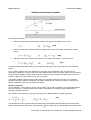
Anisotropy
Although Triwaco assumes that transmissivities and permeabilities of all aquifers are by default isotropic, the
user can define an anisotropic transmissivity (or permeability). The transmissivity (or permeability) tensor may
vary through the model area, which implies that the principal axes of the tensor can have different
orientations in different points of the model's domain.
The values in the direction of the principal axes of the transmissivity tensor are given by 'T1' and 'T2'. The
angle between the direction of 'T1' and the positive X-axis is given by ' '. Now the values of the transmissivity
components in the Cartesian coordinate system ('Txx', 'Txy', 'Tyx' and 'Tyy') are given by Mohr's circle and may
be written as:
[21]
For each element of the Finite Element Grid the values of 'T1', 'T2' and ' ' are calculated from the values in
the nodes that constitute the corner points of the element. The transformation (equations [21]) is carried out
using the average values of 'T1', 'T2' and ' '.
Phreatic conditions
Whenever the groundwater table falls below the top of the upper aquifer the aquifer is phreatic. This implies
that aquifer transmissivity becomes a function of the piezometric head 'h'.
The phreatic transmissivity is calculated by the program Flairs using the following parameters, which have to
be specified by the user:



permeability tensor, which may be anisotropic 'K' ('K1', 'K2' and '
the elevation of the base of the upper aquifer ('HB1');
the elevation of the top of upper aquifer ('HT1').
');
The elevation of the top and the base of the upper aquifer are measured with respect to the same reference
level that is used for the piezometric heads.
5 Execution of Groundwater Flow Simulations: FLAIRS and MODFLOW-27
Royal Haskoning
Triwaco User's Manual
The aquifer's transmissivity is computed with the following assumptions:

When the piezometric head is below the base of the aquifer, the aquifer is dry, hence:
[22a]

When the piezometric head is between the base and the top of the aquifer the aquifer is phreatic,
hence:
[22b]

When the piezometric head is above the top of the aquifer the aquifer is confined, hence:
[22c]
It is assumed that the phreatic surface will not fall below the base of the aquifer and reach the underlying
aquifer.
Thus, aquifer conditions may vary depending on the value of the piezometric head. The value of the
piezometric head differs for each node of the Finite Element Grid. Hence, the upper aquifer can be partly dry,
partly phreatic and partly confined at the same time. Moreover, when transient calculations are carried out,
aquifer conditions at a given location may also vary in time.
The aquifer conditions will also influence the value of the storage coefficient to be used. For a confined
aquifer the storage coefficient is defined by the elastic storativity ('S'), whereas for phreatic conditions the
storage coefficient is given by the effective porosity 'n'.
Interface conditions
The groundwater in the lowermost aquifer can be flowing over a body of a heavier, but supposedly stagnant,
fluid. For example: in coastal areas the fresh water is separated by a (relatively) sharp interface from
(relatively) stagnant salt water.
The elevation of the interface (Hi) is given according to the 'Badon-Ghyben / Herzberg' equation:
[23]
The variables 'hs' and 'h' represent the salt-water head in the stagnant salt-water body and the piezometric
head in the fresh water respectively. The parameter ' ' is a measure for the density differences between the
5 Execution of Groundwater Flow Simulations: FLAIRS and MODFLOW-28
Royal Haskoning
Triwaco User's Manual
fresh and the salt water and is defined by:
[24]
with:
the fluid density for the fresh-water body
the fluid density for the salt-water body.
For each element of the Finite Element Grid the values of 'hs', 'HB,n' and 'HT,n' are calculated from the values
in the nodes belonging to the element.
Similarly to a phreatic aquifer one can distinguish the following situations:

The aquifer is completely fresh; the interface is below the base of the aquifer, hence:
[25a]

The aquifer is partly fresh; the interface is between the top and the base of the aquifer, hence:
[25b]

The aquifer is completely salt; the interface is above the top of the aquifer, hence:
[25c]
It is assumed that the interface will not pass the top of the aquifer and reach the overlying aquifer.
Thus aquifer conditions may vary depending on the value of the piezometric head. The value of the
piezometric head differs for each node of the Finite Element Grid. Consequently, the lowermost aquifer can
be completely fresh, partly fresh and partly salt or completely salt at the same time.
The aquifer conditions will also influence the value of the storage coefficient to be used. For a completely
fresh aquifer the storage coefficient is defined by the elastic storativity ('S'). For interface conditions, with a
partly fresh aquifer, the storage coefficient is defined by '
' with 'n' representing the effective porosity.
5 Execution of Groundwater Flow Simulations: FLAIRS and MODFLOW-29
Royal Haskoning
Triwaco User's Manual
In case of a single aquifer model, both a phreatic surface and a salt-fresh water interface may appear in the
same (top) aquifer.
Note that the program Flairs should not be used for transient calculations with a salt-fresh interface, because
the salt-water body is assumed to be stagnant. In that case or if the interface passes the top of the lowermost aquifer one should use the variable density module FLAIRSVD.
5 Execution of Groundwater Flow Simulations: FLAIRS and MODFLOW-30
Royal Haskoning
Triwaco User's Manual
5.4 Executing model simulations with MODFLOW
5.4.1 Introduction
Groundwater flow calculations can be carried out in a way similar to the calculations with the standard
Triwaco programs. In stead of running the program Flairs the program runMFfli will be called. This program
reads the standard input file flairs.fli, translates the input into ModFlow input files, runs ModFlow with these
files and writes and converts the standard ModFlow output back into standard Triwaco output format
(default file name flairs.flo). All ModFlow files remain present, so the user can not only check the regular log,
print and output files but also the ModFlow output flairs.out. The ModFlow input files all have standard file
names, which differ only by their extension, e.g. FLAIRS.BAS, .BCF, .DRN, .RIV, .GHB, .RCH, .PCG et
cetera.
There are however some restrictions in using ModFlow. The program runMFfli does not support at this time
all top systems, boundary conditions and river or source types which can be defined for Flairs. The program
however does support the following:






Steady state calculations for multi-layered aquifer systems, both semi and fully 3D.
Top system type 1, 2, 4 and 11, defined by the RCH, GHB and DRN packages.
Rivers of type 1 (RAx=1), defined by the GHB and DRN packages.
Rivers to be defined by the RIV and DRN packages (special type RAx=3).
Constant head boundaries (IBx=0), defined by constant head cells.
Given rate abstraction wells (ISx=0), defined by the WEL package.
For transient calculations and implementation of other boundary conditions the user should modify the
ModFlow input files or contact the Triwaco Help Desk assistant.
5.4.2 Using the Simulation Package MODFLOW
Groundwater flow calculations can be carried out in a way similar to the calculations with the standard
Triwaco programs. One only has to define ModFlow as the simulation package in the Grid data set info
window by selecting ModFlow in the Progam Group pull down menu. Triwaco will then use Monet for
generating the finite difference grid and ModFlow-96 to calculate grondwaterflow.
Monet is used as two-dimensional mesh generator for Triwaco when the simulation is carried out with
ModFlow. Monet produces a Tesnet compatible output file with a number of additional sets that facilitate the
generation of Modflow datafiles.
1. Mesh refinement around sources in the input file is ignored.
2. Density polygons may be digitised clockwise or counter clockwise and do not have to appear in a
particular order in the input file
5 Execution of Groundwater Flow Simulations: FLAIRS and MODFLOW-31
Royal Haskoning
Triwaco User's Manual
3. The density of the polygon with the largest area is used as the default area constraint for the entire
model
4. Rivers that cross the boundary more than once will be split into separate rivers with the same river id.
Monet first reads the boundary, river and source input and snaps all input points that are closer to each other
than EPFIX. Set EPFIX to 0 if you don't want nodes to be snapped. The intersection points with the rivers and
the boundary are calculated and the rivers and sources are clipped to the boundary polygon. Next, the
density polygons are read and sorted on de-creasing area. After reading all input, the smallest rectangle
enclosing the boundary polygon is calculated and rectangular grid cells are created within the enclosing
rectangle. The distance between the gridlines is determined by the node distance of the density polygons.
Finally, the centers of the grid cells are calculated and used to generate a triangular mesh.
5.4.3 Simulation options
After allocation of the values for all model parameters one may start the groundwater flow calculations. First,
selecting 'Calibration' 'Options' from the menu bar, the 'Calculation options' dialog box is opened.
In this dialog box the user specifies parameters related to the iteration process:
Description
Inner iteration
Outer iteration
Convergence
Function
Sets the maximum number of inner iterations
Sets the maximum number of outer iterations
Sets the criterion for confergence
Relaxation
Sets the relaxation factor
Apart from the maximum number of iterations, the user has to specify a criterion for convergence. The
program checks whether or not differences are less than the criterion specified. The initial conditions for each
outer iteration depend on the head change between (outer) iterations. In case of badly converging systems a
relaxation factor may be defined. In that case the head change between (outer) iterations is multiplied with
the relaxation factor. This causes a more stable iteration process but also results in smaller head changes,
thus requiring more iterations to reach a solution.
ModFlow calulation settings
The program runMFfli assumes that Version 2 of the Preconditioned Conjugate Gradient solver is used
(PCG2) in the ModFlow calculations. The parameters for this solver are partly fixed and partly read from the
flairs.fli input file. The parameters read from the input file are the maximum number of inner and outer
iterations (IImax and IOmax, set 14 of the input file), the relaxation factor (Rrlax, set 2 of the input file) and the
criterion of convergence (EPS, set 14 of the input file)
Note that the parameter EPS specified in the calculation options window has a quite different meaning within
Triwaco than the criterion for convergence within ModFlow. The parameter EPS is now used to define the
(physical) closure limits, which depend on the system units. The head change criterion HCLOSE has the
dimension of [Length] and the residual criterion of convergence RCLOSE the dimension of [Length^3/Time].
Where ModFlow generally uses the system units meters and seconds most Triwaco users employ the
system units meters for length and days for time. Therefore the recommended value of 0.01 or 0.001 for the
head change criterion HCLOSE can be adopted. However, because the residual criterion for convergence
RCLOSE depends on the time unit, the recommended value (equal to HCLOSE) should be multiplied by
86400 (the number of seconds per day).
5 Execution of Groundwater Flow Simulations: FLAIRS and MODFLOW-32
Royal Haskoning
Triwaco User's Manual
The program runMFfli reads the value for HCLOSE from the input file and computes the value for RCLOSE
afterwards.
ModFlow
PCG2
parameter
MXITER
Description and source
ITER1
Maximum number of inner iterations per time step.
Taken from .FLI file (IOmax, usually <=30 for linear problems, and 3 à 10 for non-linear
problems).
Type of preconditioning to be used.
Fixed at 1 (Modified, Incomplete Cholesky method)
Head change criterion for convergence.
Taken from .FLI file (EPS; Usually 0.01 or 0.001)
Residual criterion for convergence.
Computed from HCLOSE: RCLOSE = 86400 * HCLOSE
Relaxation parameter.
Taken from .FLI file (Rrlax, Usually set to 1; however, a value of 0.97 to 0.99 may
prevent zero divide and non-diagonally dominant matrix errors in case rewetting is
active).
Not used for NPCOND=2.
Fixed dummy value
Printout interval.
Fixed to 1
Print type.
Fixed to -1 (number of iterations, head changes and residuals are printed).
Recalculation Cholesky decomposition.
Fixed at 0 (recalculated each outer iteration)
NPCOND
HCLOSE
RCLOSE
RELAX
NBPOL
IPRPCG
MUTPCG
IPCGCD
Maximum number of outer iterations per time step.
Taken from .FLI file (IImax usually less than 100 will be enough).
5.4.4 Executing the model simulation
For starting the model calculations one first selects 'Generate input' from the Calibration pull down menu bar.
This will generate the input file needed (flairs.fli). This input file may be viewed or edited selecting 'View'
'Input' from the pull down menu. The input file contains all parameters needed for the calculations.
Selecting 'Run Simulation' from the Calibration pull down menu starts model simulations. A window, showing
the calculation process (RunMFli and a dosbox with ModFlow) will be displayed and the program will be
added to the tasks window. Once the calculation has stopped the 'Result parameters' Tab-sheet will be
updated. After the first run this Tab-sheet will be added to the 'Calibration data set'. If a 'calibration file' has
been defined, the program automatically compares the calculation results with the observed heads/fluxes.
5 Execution of Groundwater Flow Simulations: FLAIRS and MODFLOW-33
Royal Haskoning
Triwaco User's Manual
The simulation program produces different types of output files. RunMFli writes and converts the standard
ModFlow output back into standard Triwaco output format (default file name flairs.flo). All ModFlow files
remain present. Some of these files contain information on the calculation process, errors encountered,
(flairs.flg) others contain the calculation results using various formats (flairs.flp, flairs.flo).
5.4.5 Viewing output results (maps)
Selecting 'View' 'Results' from the Calibration pull down menu starts the graphical presentation program
TriPlot, loads the grid information and displays the layout of the model area. Now the user can contour or
classify the result parameters and view the results in plane view or can select a cross-section of the model
area.
Alternatively, the user can select one of the parameters from the 'result parameters' sheet and viewing the
parameter separately selecting 'View' 'Adore' from the Parameter pull down menu or 'View Adore file' from
the pop-up menu (right hand mouse button). Adding other parameters (selecting 'Param' 'Load' from the
TriPlot menu bar) gives the user the opportunity to compare result parameters with model input parameters.
5.4.6 Output data description
The output description of Triwaco files is described in section 5.2.7. The simualtion results are saved in bot
Triwaco standard output files (flairs.flo, flairs.flg and flairs.flp) but also in the standard ModFlow output file
format (flairs.out). The output of ModFlow files is described in the standard ModFlow manual provided by the
USGS.
5.4.7 MODFLOW parameter handling by TRIWACO
The standard input file, with the default model parameters, may be used without any modifications. In that
case the program will generate ModFlow input files that are compatible with the Triwaco stratification of
aquifers with horizontal groundwater flow and aquitards with vertical flow. The prevailing parameters are the
aquifer transmissivity and the hydraulic resistance of the intermediate confining layers. The depths and
thickness of the various layers are not taken into account other than by their hydrogeological properties.
Fully 3D
For combined groundwater flow and transport modeling, however, it is usually preferred to create a fully 3dimensional model, taking all layer boundaries into consideration. The program runMFfli will translate the
input file to a fully 3-D ModFlow model if the following Triwaco parameters are used, in stead of the
transmissivity TXx:
•
•
•
the aquifer's permeability PXx,
the aquifer's top elevation RLx and
the aquifer's base elevation THx.
5 Execution of Groundwater Flow Simulations: FLAIRS and MODFLOW-34
Royal Haskoning
Triwaco User's Manual
The parameters representing the aquitards don't need any modification. The input file can be generated as
usual selecting 'Generate input' from the 'Calibration' pull down menu. It is recommended to check the input
file and to remove the lines defining the parameter TXx, which may appear in the input file if both TXx and
PXx are defined in the same data set.
Recharge and rewetting
The recharge is computed for each cell from the corresponding Triwaco parameter (generally top system
parameter RP1). By default recharge is supposed to take place in the uppermost active cell (NRCHOP = 3 in
the RCH1 package).
Unlike Triwaco ModFlow allows cells to go dry if the water table falls below the base of the aquifer (in
Triwaco only the uppermost layer may become dry, resulting in a zero value for this aquifer's transmissivity).
For cells that become dry the value of 1.0 E+32 is assumed, signifying the cell is inactive and does not
participate in the groundwater flow.
However, whenever the water table rises above the aquifer's base elevation the cell should participate in the
groundwater flow again. This process is called 'rewetting' and is supposed to be active. Values for the
rewetting threshold and the frequency of updating are fixed.
Rivers
Streams and rivers are usually defined by line elements and will be converted to a combination of ModFlow's
DRAIN- and GHB-package, thus accounting for differences in drainage and infiltration resistances. Generally
this approach will be permitted as long as the groundwater head does not fall below the bottom level of the
river. However, in cases very low groundwater heads may be expected the linear relation between the head
difference and the infiltration flux is not valid any more. In that case the RIV-package should be used in stead
of the GHB-package.
The user can specify which line elements are to be defined by the RIV-package by adding the parameter
BRx and modifying Rax.
For those rivers that should be converted to the RIV-package, the river activity parameter RAx should be set
to 3. In addition the parameter BRx is added, representing the river's bottom elevation. This parameter can
be added selecting 'Add' 'User Defined' from the 'Parameter' pull down menu and filling in the parameter
definition window. After having allocated all parameters the input file can be generated as usual.
5 Execution of Groundwater Flow Simulations: FLAIRS and MODFLOW-35
Royal Haskoning
Triwaco User's Manual
Translation of model parameters
For the definition of the upper boundary condition Triwaco uses the so-called top systems together with line
elements or rivers. The top system parameters are distributed parameters, defined in each node of the grid
and represent the node's influence area. The river parameters, representing line elements, are defined in
each river-node and are valid for an area equal to the length of the river stretch multiplied by the river width,
which is generally considerably smaller than the river-node's influence area.
In ModFlow the upper boundary condition is defined for cells belonging to the uppermost layer, regardless of
the fact whether the boundary condition represent a distributed parameter or a line element. The area
represented is accounted for in the conductance parameter (Cond).
The following ModFlow packages are used to define the upper boundary condition:
Code
RCH
GHB
Package
Recharge package:
General Head Boundary
Input parameter
RECH
Cond
HBND
[L3/T]
Q = Cond * (HBND - HCELL)
DRN
RIV
dimension
[L/T]
[L2/T]
[L]
Drain package
HDRAIN
[L]
Q = Cond * (HBND - HCELL)
Q=0
Cond
{HCELL > HBND}
{HCELL
HBND}
[L2/T]
[L3/T]
River Package
RBOT
[L]
HRIV
[L]
Cond
{HCELL > RBOT}
{HCELL
RBOT}
[L2/T]
[L3/T]
Q = Cond * (HRIV - HCELL)
Q = Cond * (HRIV - RBOT)
Where in Triwaco a distinction can be made between an infiltration and a drainage situation, the GHB, DRN
and RIV package do not differentiate between these two situations. The conductance is supposed to be a
constant, regardless of the prevailing condition. Therefore, the upper boundary condition in Triwaco, be it a
top system or a river, is translated into a combination of the ModFlow boundary packages mentioned. The
precipitation excess or groundwater recharge is simulated using the RCH package.
The conductance of the GHB or RIV package is based on the infiltration resistance of top system or river,
whereas the conductance of the DRN package is based on the drainage resistance. Thus, the program
runMFfli will interpret the top system and river information and generate the corresponding ModFlow
packages:
Triwaco Top system
Precipitation excess
RP1
IR = 1
IR = 2
Controlled water level
RP1
Hydraulic resistance Drainage resistance RP2
RP3
IR = 4
Not yet fully functional
RP1 - RP13
IR =11
Precipitation excess
RP1
Hydraulic resistance
RP2 RP3 RP4
Drainage resistance
RP5
Infiltration resistance
Controlled water level
River
River water level
HRx
River width Drainage resistance
RWx
Infiltration resistance
CDx
CIx
ModFlow packages
RCH
GHB
GHB and DRN
GHB and DRN or RIV and DRN
5 Execution of Groundwater Flow Simulations: FLAIRS and MODFLOW-36
Royal Haskoning
Triwaco User's Manual
5 Execution of Groundwater Flow Simulations: FLAIRS and MODFLOW-37
Royal Haskoning
Triwaco User's Manual
5.4.8 Command line calls
RUNMFli
Program for the generation of ModFlow model input files and for carrying out groundwater flow calculations
with ModFlow. Calculation results are converted to a Triwaco output file (flairs.flo).
The command call is similar to that for the standard Triwaco groundwater flow module FLAIRS.
A standard input file (flairs.fli) must be generated from the TriShell. Also, a standard grid file (grid.teo) is
required. Output will be written to files: flairs.flo, flairs.flp and flairs.log. If no arguments are given the
program opens in Windows mode. The appropriate input files (grid.teo, flairs.fli and calib.chi ) can be
selected and the program may be run using the pull-down menus.
Command line call:
RunMFfli.exe set-dir grid-dir flairs.fli [calib.chi]
No options are available.
Example:
RunMFfli C:\Projdirs\Modflow C:\Projdirs\Monet flairs.fli
MFU2FLO
Program for the conversion of ModFlow output to a standard Triwaco output file (flairs.flo). The existence of
a MODFLOW compatible grid file is required.
The program searches the working directory (set-dir) for a MODFLOW output file with the same name as the
input file mentioned on the command line.
Command line call:
MFu2Flo.exe set-dir grid-dir flairs.fli [calib.chi]
No options are available
Example:
MFu2Flo C:\Projdirs\Modflow C:\Projdirs\Monet flairs.fli
5 Execution of Groundwater Flow Simulations: FLAIRS and MODFLOW-38