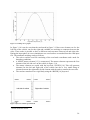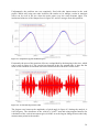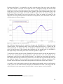
1
2008:084 CIV
MASTE R’S THESIS
Simulation of complete vehicle
dynamics using FE code Abaqus
Andreas Hellman
MASTER OF SCIENCE PROGRAMME
Mechanical Engineering
Luleå University of Technology
Department of Applied Physics and Mechanical Engineering
Division of Functional Product Development
Universitetstryckeriet, Luleå
2008:084 CIV • ISSN: 1402 - 1617 • ISRN: LTU - EX - - 08/084 - - SE
Abstract
Due to high costs when developing new vehicle models, computer simulations of vehicle
dynamics become more and more important in the product development process. Vehicle
dynamics is today a narrow area on the market, which means that it is uneconomic for most
small companies to own required licenses for these software’s since they only use them
temporary. Software used in structural analysis are much more common in the industry today
and simulating vehicle dynamics with this kind of software could result in large economic
savings and new possibilities. All commercial Finite Element (FE) codes do not have the
possibility to perform Multibody System Analysis (MBS), i.e. the movement of the body is
large compared to it own dimensions. A FE code that has this functionally is Abaqus.
This thesis work investigate the possibility to perform handling and ride simulations in
Abaqus, to see if the FE approach can present similar results as the MBS best practice. As
reference for validation of the results ADAMS/Car from MSC.Software was chosen because
it is one of the most common software on the market today used for vehicle dynamic
simulation. Handling simulations of vehicles mean different types of curved maneuvers
during different circumstances. Ride simulations of vehicles imply investigation of influences
from roughness in the road causing vibrations in the vehicles.
A full vehicle model of a Volvo S40 is modeled and simulated in both Abaqus and
ADAMS/Car and the results are compared towards each other. How the models layout and
simulation should be built up in Abaqus is investigated to get a structure that is as good as
possible for the models. To accomplish solving such a complex problem a carefully planned
strategy is required and for that purpose the Crawl-Walk-Run strategy has been used.
From the results it is concluded that Abaqus can be a good alternative to use when simulating
vehicle dynamics. Using Abaqus works fine for simple ride maneuvers but to make it possible
to perform handling simulations it is required to incorporate working tire models. The
agreement of the results between Abaqus and ADAMS/Car is very good and accurate enough
to start using Abaqus for solving real engineering problems. Still, we need to make
improvements of the models to get even better agreement.
2
Sammanfattning
På grund av höga kostnader för att utveckla nya fordonsmodeller så blir datorsimuleringar av
fordonsdynamik allt viktigare i produktutvecklingsprocessen. Fordonsdynamik är i dag ett
smalt område på marknaden, vilket innebär att det är oekonomiskt för de flesta mindre företag
att äga licenser för de programvaror som krävs för dessa simuleringar då de endast används
tillfälligt. Program för att beräkna hållfasthet är betydligt vanligare ute i industrin idag och
om möjligheten fanns att simulera fordonsdynamik med hjälp av en sådan programvara skulle
detta kunna möjliggöra stora besparingar och nya möjligheter. Alla kommersiella
hållfasthetskoder har inte funktionaliteten att räkna stelkroppsdynamik dvs när en kropps
rörelser är stora i relation till dimensionerna på delarna. En hållfasthetsprogramvara som har
detta inkluderat är Abaqus.
Examensarbetet undersöker om det är möjligt att göra handling och åkkomfortsimuleringar i
Abaqus som ger lika trovärdiga resultat som i ett för ändamålet anpassat program. Som
referens har ADAMS/Car från MSC.Software valts pga. av att det är en av de vanligaste
programvaror som används idag inom fordonsdynamiska beräkningar. Handlingsimulering av
fordon innebär olika typ av kurvtagningsmanövrar. Åkkomfortsimulering innebär simulering
av vad olika ojämnheter i vägen ger upphov till för vibrationer.
En helbilsmodell av Volvo S40 modelleras och simuleras i både Abaqus och ADAMS/Car
och resultaten jämförs mot varandra. I Abaqus har även layouten på hur modeller och
simuleringar skall byggas upp för att möjliggöra en så bra struktur av filerna som möjligt
undersökts. För att kunna lösa ett så här pass komplext problem och få goda resultat är en väl
genomtänkt strategi nödvändig och för detta ändamål har Crawl-Walk-Run strategin använts.
Från resultatet kan slutsatsen dras att Abaqus kan bli ett fullgott alternativ till simuleringar av
fordonsdynamik. Det fungerar bra för att simulera enkla åkkomfortsimuleringar men för att
möjliggöra handlingsimuleringar krävs vidare arbete för att utveckla fungerande
däckmodeller. Överensstämmelsen mellan resultaten från Abaqus och ADAMS/Car är god
och tillräckligt noggrann för att börja användas till att lösa verkliga problem. Fortsatt
förbättring i överensstämmelsen mellan programmen är något för framtida arbete.
3
Preface
This is the final report of the master thesis project “Simulation of complete vehicle dynamics
using FE code Abaqus” conducted at Caran between August 2007 and December 2007. The
thesis work was examined at the Department of Applied Physics and Mechanical Engineering
at LTU with examiner Professor Tobias Larsson and supervisor PhD student Mikael Nybacka,
both from the Division of Functional Product Development. The work was conducted and
carried out at Caran in Gothenburg, in the Dynamics department, with company supervisor
Bengt Lennartsson.
I would not have been able to carry out this thesis project without the help and assistance from
a number of people:
Bengt Lennartsson
Mikael Nybacka
Tobias Larsson
Jonas Dyberg
Supervisor, Caran AB
Supervisor, Luleå University of Technology
Examiner, Luleå University of Technology
SIMULIA Scandinavia
Thank you for your support.
Finally I would like to extend my thanks to everyone at Caran Dynamics for their support and
help with my thesis work.
4
Contents
Abstract ...................................................................................................................................... 2
Sammanfattning ......................................................................................................................... 3
Preface........................................................................................................................................ 4
1 Introduction ............................................................................................................................. 7
1.1 Background ...................................................................................................................... 7
1.2 Goal .................................................................................................................................. 8
1.3 Software ........................................................................................................................... 8
2 Previous work.......................................................................................................................... 9
2.1 Simulation theory ............................................................................................................. 9
2.1.1 Static analysis............................................................................................................ 9
2.1.2 Dynamic analysis .................................................................................................... 10
2.2 Dominant software approaches ...................................................................................... 12
2.2.1 Abaqus..................................................................................................................... 12
2.2.2 ADAMS .................................................................................................................. 12
2.2.3 CarSim..................................................................................................................... 12
2.2.4 Tesis DYNAware .................................................................................................... 13
2.3 Example pick-up Truck.................................................................................................. 13
2.4 Tire interface for Abaqus ............................................................................................... 14
2.5 Vibration rig in Abaqus.................................................................................................. 14
2.6 Suspension models ......................................................................................................... 16
2.6.1 Front Suspension ..................................................................................................... 16
2.6.2 Rear Suspension ...................................................................................................... 16
2.7 Connectors in Abaqus .................................................................................................... 17
2.7.1 MPC ........................................................................................................................ 17
2.7.2 Connector elements ................................................................................................. 17
3 Work...................................................................................................................................... 19
3.1 The ideal solution for simulating vehicle dynamics....................................................... 19
3.2 The pick-up truck ........................................................................................................... 20
3.3 Building the Abaqus model............................................................................................ 20
3.3.1 Approach ................................................................................................................. 20
3.3.2 Coordinate system definition .................................................................................. 21
3.4 The Abaqus model ......................................................................................................... 22
3.4.1 Body and general parts............................................................................................ 22
3.4.2 Front suspension...................................................................................................... 23
3.4.3 Rear suspension....................................................................................................... 24
3.5 Measurements................................................................................................................. 25
3.6 Simplifying and simulation of the simplified model...................................................... 25
3.6.1 Static simulation...................................................................................................... 26
3.6.2 Dynamic simulation ................................................................................................ 26
3.7 Implementation of tire model ......................................................................................... 27
3.8 Full vehicle analysis ....................................................................................................... 27
3.8.1 Setup for full vehicle simulation ............................................................................. 28
3.8.2 Building the road profile ......................................................................................... 29
3.9 Validation approach ....................................................................................................... 31
3.10 Building the ADAMS/Car model................................................................................. 32
3.10.1 Front suspension.................................................................................................... 33
3.10.2 Rear control blade suspension............................................................................... 33
3.10.3 Body, steering and powertrain subsystems ........................................................... 34
5
3.10.4 Tires....................................................................................................................... 34
3.10.5 Complete vehicle model........................................................................................ 34
3.10.6 Road profile........................................................................................................... 34
3.11 Simulating the ADAMS/Car model ............................................................................. 35
4 Results ................................................................................................................................... 36
4.1 Simulation of the pick up truck ...................................................................................... 36
4.2 Full vehicle simulation ................................................................................................... 36
5 Discussion and conclusion .................................................................................................... 40
5.1 Error ............................................................................................................................... 41
5.2 Difference between using Abaqus and ADAMS/Car .................................................... 41
6 Future work ........................................................................................................................... 43
6.1 Model agreement........................................................................................................ 43
6.2 Future development.................................................................................................... 43
7 References ............................................................................................................................. 45
Appendix A Results ................................................................................................................. 47
6
1 Introduction
1.1 Background
Due to high costs when developing new vehicle models, computer simulations of vehicle
dynamics become more and more important in the product development process. Vehicle
dynamics is today a narrow area on the market, which means that it is uneconomic for most
small companies to own required licenses for these software’s since they only use them
temporary. Software used in structural analysis are much more common in the industry today
and simulating vehicle dynamics with this kind of software could result in large economic
savings and new possibilities. Why not simulate vehicle dynamics with FEM analysis
software which most of the middle to larger companies already have licenses to use and staff
that are familiar with? This is the question that the thesis project focuses on.
In the job description from Caran it was desired that the FEM program Abaqus should be
used. Other large FEM software’s on the market are for example Nastran [1], Ansys [2] and
LS-DYNA [3].
If companies are willing to invest in a vehicle dynamics software their demand is most often
to get a whole simulation package. Due to the high license costs the companies want to be
able to do as many simulations as possible in one software. If Abaqus should be a real
alternative to the existing software’s on the market it must be possible to perform highly
desired handling simulations. This does not mean that for example ride simulations are not
important but a single simulation type cannot make software competitive on the market. If
software has the possibility to perform a handling simulation it is common that it can perform
the other analysis types that is simpler, such as simulations of a single front suspension.
Because of the reason to fully investigate the possibilities to perform vehicle dynamics
simulation in Abaqus a handling simulation is chosen.
7
1.2 Goal
The main purpose of this thesis work is to examine the possibility to perform vehicle
dynamics simulations of vehicle handling in FEM software Abaqus and see if this software
will give reliable results similar to market leading software.
1.3 Software
Ansa [4] v12 has been used as pre-processor for building, meshing and post FE models to
Abaqus input files. For the simulations Abaqus v6.7 has been used. Results and visualization
of the results has been made in µETA [4] v5. Adams 2005 r2 with ADAMS/Car module has
been used to build a reference to validate the results. Matlab v7.1 [5] has been used for
plotting and generating road profiles.
8
2 Previous work
To get a better understanding of the problem, to learn more about simulation of vehicle
dynamics and to get an insight of what has been done in different aspect of simulation of
vehicle dynamics in Abaqus a literature study was conducted. Different types of elements and
important building blocks to use in Abaqus were also studied.
A benchmark of the existing dominating software’s on the market used for vehicle dynamics
was performed. The front and rear suspension of the Volvo s40 was investigated to get a basic
understanding before starting the project.
2.1 Simulation theory
This section describes the theory for solving different types of simulations in Abaqus. These
simulation techniques will further on be used to solve vehicle dynamic problems. More in
detail information about the simulation techniques are available in Getting Started with
Abaqus: Interactive Edition [6].
2.1.1 Static analysis
A static analysis is sufficient if the interest is to investigate the long-term response of a
structure to applied load and the inertia effects can be neglected. The equation of equilibrium
governing static linear problems is:
KU = R
Where
(1)
K are the elemental stiffness matrix
R is the external load vector
U is the displacements
The problem can be both linear and nonlinear. Nonlinearities can arise from largedisplacement effects, material nonlinearity, and/or boundary nonlinearities such as contact
and friction. If the problem is nonlinear Newton’s method will be used to solve equation 1.
9
2.1.2 Dynamic analysis
Contrary to the static analysis a dynamic analysis has load and responses that vary with time
and the duration of loads are small. More in detail information about the dynamic analysis
techniques are available in Getting Started with Abaqus: Interactive Edition [6].
When the inertia effects in a system are important a dynamic analysis must be performed,
Abaqus has several methods for solving such problems. When nonlinear dynamic response is
studied direct integration must be used. Abaqus can use both implicit direct integration and
explicit direct integration.
The equations of equilibrium governing the nonlinear dynamic response of a system of finite
elements are:
∗∗
∗
M t U + C tU + tK tU =t R
(2)
∗
C U + KU = I
M, C, tK are the mass, damping and elemental stiffness matrices.
t
R is the external load vector
Where:
(3)
∗
I is the internal forces and is the sum of C U + KU ,
t
∗
∗∗
U , tU , tU are the displacements, velocity and acceleration vectors of the finite
Assemblage at time “t”
For solving the system off differential equation described in equation 2, direct integration is
used. That means that prior to the numerical integration; no transformation of the equations
onto a different form is carried out. The application of this method is based on two ideas:
•
•
Trying to satisfy equation 2 only at discrete time intervals “∆t”, instead of any time “t”
Assume the variation of the displacements, velocities and accelerations within each
time interval “∆t”. Obviously, the choice criteria on these assumptions determine the
accuracy, stability and cost of the solution procedure.
The direct integration procedure uses the mass, damping, and stiffness matrices in equation 2
assembled and the equation of dynamic equilibrium is solved at each point of time. If the
problem is linear better methods for solving equation 2 are available, not all the equations
need to be solved for each time. That makes direct integration more expensive than other
methods.
2.1.2.1 Explicit method
In this method, known also as central difference method, the kinematic conditions at one
increment are used to calculate the kinematic conditions at the next one. At the beginning of
each increment the program solves the dynamic equilibrium with respect to accelerations
according to equation 4.
∗∗
MU = R−I
(4)
10
Since the acceleration of any node is determined by its mass and the net force acting on it the
nodal calculations is very inexpensive. The accelerations are integrated through time using the
central difference rule, which calculates the change in velocity from the middle of the
previous increment to determine the velocities at the middle of the current increment. After
that the velocities are integrated through time and added to the displacement at the beginning
of the increment to determine the displacements at the end of the increment. Thus satisfying
dynamic equilibrium at the beginning of the increment again provides the accelerations for the
new loop.
The explicit method requires small time increment to produce accurate results depending on
that the accelerations in the central difference formula are assumed to be nearly constant.
Simulations generally take on the order of 10 000 to 1 000 000 increments, but the
computational cost per increment is relatively small as explained previously.
To know that the simulations provide accurate results the time step must be smaller than a
critical value ∆tstable known as the stability limit (without damping):
Δt stable =
Where
2
ω max
(5)
ωmax is the highest frequency in the system
An approximation to the stability is written as the smallest transit time of a dilatational wave
across any of the elements in the mesh:
Lmin
(6)
cd
Where Lmin is the smallest element dimension in the mesh and cd is wave speed of the
material.
Δt stable ≈
A big advantage with the explicit method is the ability to define and manage contact problems
in a good way.
2.1.2.2 Implicit method
The general direct-integration method provided in Abaqus/Standard, called the HilberHughes-Taylor operator [6], is an extension of the trapezoidal rule. In this method the
integration operator matrix must be inverted, and a set of simultaneous nonlinear dynamic
equilibrium equations must be solved at each time increment. This solution is done iteratively
using Newton's method [6].
This nonlinear equation solving process is expensive; and if the equations are very nonlinear,
it may be difficult to obtain a solution. However, nonlinearities are usually accounted more
simply in dynamic situations than in static situations, because the inertia terms provide
mathematical stability to the system. Thus, the method is successful in all but the most
extreme cases.
To control the accuracy in the solution, the method of half-step residual is used. It is based on
calculating the equilibrium residual error (out-of-balance forces) halfway through a time
increment. If the half-step residual is small enough the calculation will continue.
11
A big advantage of step-by-step solution scheme base on this integration is that it can be used
for solving both static and dynamic problems, whereas the central difference method solution
could not be used if mass and damping effects are neglected.
2.2 Dominant software approaches
In this section information about several software’s is presented. Abaqus is described and
after that information are given about the most common software’s on the market today used
for vehicle dynamic simulations.
2.2.1 Abaqus
Abaqus [7] is one of several large software suppliers on the market today for solving problem
in multiphysics. Starting with Abaqus V2 (in 1979), Abaqus/Aqua simulates hydrodynamic
wave loading on flexible structures for offshore pipelines. Through the years additional
multiphysics capabilities have been added, such as fluid, thermal, and electrical couplings, to
name a few.
As seen in [7] the Abaqus product suite consists of three core products: Abaqus/Standard,
Abaqus/Explicit and Abaqus/CAE. Abaqus/Standard is a general-purpose solver that uses
traditional implicit integration scheme to solve finite element analyses. Abaqus/Explicit uses
explicit integration scheme to solve highly nonlinear transient dynamic analysis. Abaqus/CAE
provides an integrated modeling (preprocessing) and visualization (postprocessing)
environment for the analysis products.
2.2.2 ADAMS
MSC.ADAMS [8] started as a spin off from the University of Michigan and is today one of
the dominating software on the market for Multibody System Analysis (MBS). The character
for MBS is that the components’ overall motion is large compared to their dimensions.
ADAMS is a big family with interactive simulation software for solving problems in a very
large range of topics as train, aircraft, aeronautics and automotives. In the application
ADAMS/Car the most common vehicle dynamics problem can be solved such as handling
and ride behavior.
The interface can be chosen between graphic and text based. ADAMS has its own
postprocessor for reviewing data and graphics. Implicit and explicit integration methods are
supported and a wide range of interpolation methods are available.
2.2.3 CarSim
Similar as ADAMS, CarSim [9] provided by Mechanical Simulation Corporation started as a
spin of from the University of Michigan. CarSim use a different solver approach than
ADAMS, instead of modeling all parts of the vehicle you use data acquired from Kinematics
and Compliance (K&C) tests instead. This speeds up the simulation considerably.
CarSim is used to simulate the dynamic behavior of racecars, passenger cars, light trucks, and
utility vehicles. Versions used to simulate behavior of trucks and motorcycles are also
available. CarSim is a complete package with everything needed to simulate vehicle
dynamics, such as tire models and postprocessor to review data.
12
2.2.4 Tesis DYNAware
Tesis DYNAware [10] is provided by the German company Tesis Group and consists of four
different products: enDYNA simulates combustion engines, veDyna simulates vehicle
dynamics, Realtime Brake Hydraulics is used to simulate brake hydraulics and
DYNAanimation visualizing results.
veDYNA has several different product levels and model enhancements with different cost
levels. The cost is somewhere about the same level as CarSim. Like CarSim data acquired
from Kinematics and Compliance (K&C) tests are used.
2.3 Example pick-up Truck
In Vehicle analyses in Abaqus Example Problem Manuals v6.7 chapter 3.2 [11] simulation of
a pick-up truck is described. The model shown in figure 2.1 was obtained from the Public
Finite Element Model Archive of the National Crash Analysis Center at George Washington
University and contains approximately 55 000 elements.
Different vehicle dynamics simulations are performed in chapters 3.2.1 -3.2.3 [11] with
different level of complexity. In chapter 3.2.1 in [11] an inertia relief and dynamic simulation
are described where the simulation starts with gravity loading and continue with acceleration
to a constant speed and after that brake until the pick-up truck remain stationary. The
simulation is rather simplified because the tires are modeled as springs between the spindles
on the suspension and the ground.
Figure 2.1: The pick-up truck [11]
In chapter 3.2.2 in [11] a substructure analysis is described where the goal is to run the truck
over some road obstacles. First the initial stress in leafs and struts for the gravity load are
calculated in several separate analysis. After that the main simulation starts where the truck
13
goes over different obstacles. The tire model is a simplified Calspan1 model that only takes
into account the radial forces in the tires and not the lateral forces etc.
By using the substructure method the speed of the simulation can be increased compared to
the full dynamic simulation in chapter 3.2.1 [11]. To further speed up the simulation, display
bodies are used instead in chapter 3.2.3 [11].
2.4 Tire interface for Abaqus
In November year 2003 a company named TNO from Netherlands presented a project [12] on
Abaqus Users’ Conference2 that they had carried out to make a tire interface between MFtyres3 and Abaqus. With that interface it should be possible to perform rolling tire vehicle
dynamics simulations in Abaqus. According to the documentation [12] the interface should
work both for Abaqus Standard and Explicit.
2.5 Vibration rig in Abaqus
In 2003 an internal project at Caran started to investigate the possibility to simulate vibrations
in a full vehicle model in Abaqus software. A model of a Volvo s40 have been built and is
shown in figure 2.2 acquired from FEM pre processor Ansa. The original model was obtained
from MSC ADAMS/Car with data for the bushings, spring curves and so on kept as the
default values in ADAMS. The Abaqus model consists of 204 nodes and 385 elements where
all the structural elements consist of beam elements. The beam elements for the suspension
and chassis are modeled with a high stiffness material to get them as near rigid elements as
possible. This because in vehicle dynamics the main interest is not the internal deformation
and tensions in the individual parts for example the suspension arms. The focus is instead on
different parameters like the roll angle of the chassis and forces acting on the tires and joints.
Because the model consist of beam elements it is very fast to compute and will not require
modeling techniques like substructure and display bodies as used in the example truck
described in chapter 2.3 to get reasonable simulation time.
Connector elements of different types were used for the bushings and joints between the rigid
parts, for further explanation of connector elements see chapter 2.7.
1
Tire friction model common used in vehicle dynamics simulations
Conference for the user’s of FEM software Abaqus
3
Tire model common used in vehicle dynamics simulations
2
14
Figure 2.2: The vibration rig in Ansa
Tires used in the model are non-rolling tires modeled with connector element between the
ground and rims. The following constants are taken in account with actual values:
•
•
•
•
•
•
Tx (longitudinal stiffness)
Ty (lateral stiffness)
Tz (vertical stiffness)
Rx (Camber torsion stiffness)
Ry (Rolling Resistance Moment)
Rz (Steering torsion stiffness)
= 341 N/mm
= 117 N/mm
= 235 N/mm
= 35120 Nmm/deg
= 17900 Nmm/deg
= 38043 Nmm/deg
Damping was also taking in account in the tire model.
The springs and dampers in the model were made of connector element only acting in the
axial direction. Forces in the springs are defined by the axial stiffness in the connector
element. The stiffness is defined as a nonlinear curve where a force is interpolated for a given
displacement, and the preload in the springs are defined by the free length parameter. Like the
springs the dampers initial condition is also defined by a curve but instead force depends on
the velocity.
15
2.6 Suspension models
The suspension system of Volvo S40 will here be explained briefly to gain a better
understanding before further reading about simulations of the model.
2.6.1 Front Suspension
The front suspension consists of a McPherson strut type seen in figure 2.3, this is the most
widely used front suspension system in cars of European origin. The system is very simple
where the strut consists of a spring and damper combination pivoted with a spherical bearing
at the lower a-arm. The strut is a fully stressed component and hold up the car. The steering
arm is connected to the spindle and when the car steer the whole strut assembly turns around
its own axle of rotation. The anti roll bar, which connects the left and right front suspension,
is connected at the strut. In figure 2.3 all the bushings with names from the original
ADAMS/Car model can be seen.
Figure 2.3: McPherson suspension model
2.6.2 Rear Suspension
The rear suspension consists of a control blade type shown in figure 2.4, which is a
combination of a multi link suspension together with a trailing arm type. One big advantage
with this suspension type is that it takes up less space and leaves more space to the interior.
The largest reason to the space saving is that the spring and damper are separate units. The
separation of the damper and spring makes it also possible to improve the geometry for ride
and handling of the car. One of the advantages with the trailing arm is that you get “anti-dive”
which mean that the car will dive less when hitting on the brakes. In the figure 2.4 all the
bushings with names from the original ADAMS/Car model can be seen.
16
Figure 2.4:Control blade suspension model
2.7 Connectors in Abaqus
To be able to build fully functional vehicle models that correspond well to real life behavior,
something is needed to bring together the different parts. In Abaqus v6.7 several different
methods are available for connecting elements or parts to each other. Only two of them will
be discussed in this thesis project: The Multi Point Constraints and the connector elements.
Detailed information about Multi Point Constraint and connector elements can be found in
Abaqus Analysis User’s Manual [13]. In the internal report “Abaqus Connector Elements”
[14] made at Caran a summary between the differences connectors and a example can be
found.
2.7.1 MPC
Multi-point constraints (MPCs) specify linear or nonlinear constraints between nodes and is
more efficient then connector elements. One disadvantage is that they eliminate degrees of
freedom at one of the nodes involved in the connection. This elimination has the advantage
that the problem size is reduced; it has the disadvantage that output and other functionality
provided with connector elements is not available.
Another disadvantage is that MPC forces are not available as output quantities and many of
the general connectors can only be used together with Abaqus/Standard.
2.7.2 Connector elements
The connector elements have two types available for different purposes. One type for twodimensional and axisymmetric analyses and one for three-dimensional analyses. Both types
have at most two nodes. The position and motion of the second node on the connector element
are measured relative to the first one. Connector elements do not eliminate degrees of freedom
and kinematic constraints are enforced with Lagrange multipliers. The Lagrange multipliers
provide constraint force and moment output.
17
The connection types are divided into three categories: basic connection components,
assembled connections, and complex connections. The basic connection components affect
either translations or rotations on the second node. A connector element may include one
translational basic connection component and/or one rotational basic connection component.
The assembled connections are constructed from the basic connection components. They are
provided for convenience and cannot be combined in the same connector element definition
with a basic connection component or other assembled connections. Complex connections
affect a combination of degrees of freedom at the nodes in the connection and cannot be
combined with other connection components. In “connection-type library” Section 25.1.4 [13]
all the different connector elements can be reviewed in detail.
18
3 Work
This chapter will explain the practical work in this thesis project. How the structure for the
models and simulations in Abaqus and ADAMS/Car is prepared and the technique to define
the models.
3.1 The ideal solution for simulating vehicle dynamics
The paper “Numerical simulation of full vehicle dynamic behavior based on the interaction
between Abaqus/Standard and explicit codes” [15] discuss the problem of choosing Abaqus
solver thorough performing vehicle dynamics simulation.
One advantage with Abaqus is that the code has the possibility to transfer information
between the different solvers in both directions. This reason makes the program very good for
investigating the possibility to simulate vehicle dynamics in FEM Software, but how would
the ideal solution look like if the advantage of each solver were used? For example, the nonlinear dynamic transient problem predicting a vehicle behavior when passing over obstacles.
The ideal solution for that problem should be to perform a static analysis (equilibrium prior to
the dynamic simulation) using an implicit code and use the implicit results as initial condition
of the dynamic analysis performed with an explicit code. This example minimizes the cost of
the simulation, taking advantage of the explicit code in rapidly transient dynamic problems
and the implicit code for simulations with longer timescales.
One other possibility is to only use the implicit method but that will not optimize the cost of
the simulation. In other cases the advantage with only using one code is that only one solver is
required which makes it cheaper and less user knowledge is required.
19
3.2 The pick-up truck
To learn about Abaqus and get an insight how the vehicle dynamics could be simulated in
Abaqus the first part of the project was spent on trying to simulate the pick-up truck from
Abaqus Example manual [11].
The main focus with the pick-up truck simulations are different compared to this project. The
difference is focusing a lot of the stress in the components, and not only on the dynamics
behavior of the vehicle. Because of that area of interest the model is large and it takes a while
to simulate.
3.3 Building the Abaqus model
This chapter explains the approach for building the Abaqus model, the coordinate definition
and the measurements that has been used.
3.3.1 Approach
When building and simulating the Abaqus model the Crawl-Walk-Run approach has been
used. This means that the complexity of the model and simulations in the beginning is low
and as the project preceded more and more complexity has been built in and added. In figure
3.1 the Crawl-Walk-Run approach is shown for the project. In the crawl phase the existing
model from the vibration project was taken and carried out some work to simplify and adapt
for this project. After, the implementation of simplified tires start and a static simulation was
performed on the simplified model. In the walk phase a dynamic simulation was carried out
for the simplified model and after that the implementation of the handling tires start.
In the run phase a full vehicle model simulation is carried out where the working full car
model assembled with the tire model was performing a dynamic simulation for a handling
manoeuvre.
The limitations of the simplified model decide how the simplified dynamic simulation has
been built up. For example it is not realizable to make a handling manoeuvre with the
simplified tires.
20
Figure 3.1:The Crawl- Walk-Run approach
3.3.2 Coordinate system definition
The global coordinate of the vehicle can be seen in figure 3.2, the z direction is pointing
upwards to the sky from the ground and the x direction is pointing to the rear of the car. The
numbers in the figure shows identifier numbers for element and nodes in the model. 1000 is
the front left tire.
1000
2000
Y
3000
There are several different coordinate systems in the model because
some elements need special coordinate systems to be defined
properly. The boundary conditions and constraints are defined as the
term “degree of freedom”. The degree of freedom 1-3 is translation in
x (longitudinal),y (lateral) and z (vertical) direction, 4-6 is rotation
around the axles x (roll),y (pitch) and z (yaw).
4000
X
Figure 3.2: Vehicle global coordinate system
21
3.4 The Abaqus model
This section will describe the strategy and building of the Abaqus model in detail and show
how all the parts are connected to each other in the physical meaning. As shown in figure 3.3
it will imply that the whole model is built up in one single input file for Abaqus. The input file
is built up in a text-based format in a text editor.
Figure 3.3: Abaqus full vehicle model built up strategy
The in real life car has both bushings4 and rigid joints used as connectors between the
different parts. Connector elements have been used in the models to reflect the bushings and
rigid joints. To reflect the rigid joints the connector element of type join has been used. For
the bushings a combination of the connector elements join and cartesian has been used, with
elastic stiffness defined as curves in all degrees of freedom.
3.4.1 Body and general parts
All parts in the model which represent the body and subframe geometry see figure 3.4 are
modeled with B31 [13] beam elements. Abaqus support rigid elements but the choice felt on
the beam elements because of the flexibility. If the beams material assigns a high stiffness
compare to the model units they will imitate a rigid element well but some computational cost
is lost. The advantage is that if the model will have bigger future flexibility because real
stiffness can be assigned to parts very simply, by changing the young modulus for the
materials.
Figure 3.4: Body and subframe parts
4
A connector with defined stiffness in all degrees of freedom.
22
The steer rack and steering column in the steering module are attached to the body. In figure
3.5 it is shown that the tie rod is connected to the steering rack with a CV joint5, and at the
other end connected to the spindle with a spherical joint.6
Figure 3.5: The steering module
3.4.2 Front suspension
The spring consists of an axial connector element with a
force curve for a given displacement, which is connected
to the body node in figure 3.6 and the strut in the other
end. The damper consists of an axial connector element
with a force curve for a given velocity and is connected to
the body through a bushing and the strut in the other end
as in figure 3.6. Because the axial element doesn’t impose
any kinematic constraints7 a cylindrical8 joint is placed
between the end nodes of the damper to simulate the rigid
behavior of the strut. The spindle, strut, tie rod and lower
control arm in figure 3.7 are modeled with B31 beam
elements. Each solid part has its own mass and inertia
defined.
Figure 3.6: The strut assembly
5
A connector with only two rotational degree of freedom
A connector with only three rotational degree of freedom
7
Any condition relating properties of a dynamic system that must hold true at all times
8
A connector with only one rotational and one translational degree of freedom
6
23
Figure 3.7: The front suspension
3.4.3 Rear suspension
In the rear suspension shown in figure 3.8 the spring consists of a connector element with a
force curve for a given displacement, which is connected to the rear subframe in one end and
to the suspension in the other. The damper consists of an axial connector element with a force
curve for a given velocity and is connected to the body through a bushing and the control
blade in the other end as in figure 3.8 The control blade and all the other rods are modeled
with B31 beam elements. In real life the control blade is made flexible but in the model it is
rigid.
Figure 3.8: The rear suspension
24
3.5 Measurements
Abaqus has a lot of opportunities to generate output from simulations. In this project outputs
to an odb database to be viewed in the postprocessor µETA, and results written to text files
are used. The wanted outputs need to be specified in the input file to the simulation with
different keywords see chapter 4.1 in Abaqus Analysis Manual [13]. Both nodes and elements
can be used for output and the choice of element, connectors, solver etc. limits which outputs
can be made.
To get a better possibility to investigate the vertical movement of the body, measurement
points above the wheel centers in front and rear were constructed as in figure 3.9. The
connection between the center of gravity (COG) and the measure points consist of B31 [13]
high stiffness beam elements, same as the structural elements. The vertical position of the
points is the same as the COG. The longitudinal position is the same as the wheel centers.
Figure 3.9: Vehicle measure points
3.6 Simplifying and simulation of the simplified model
In this stage of the process the main focus is the vehicle model and how to get a model that
has a good quality. This mean that after this phase of the project the vehicle model should be
stable to simulate and be as similar as possible to the real life vehicle. That does not include
the behavior of the car with tires, which will be implemented later on.
The first thing to do was to go through the whole vibration model and investigate how all the
parts was defined and coupled to each other. To get some kind of reference simulation the old
simulation was run.
In the vibration rig project the focus was to optimize the bushing that connects the engine to
the body. In this project that is not important and therefore the engine part was removed but
the engine mass and moment inertia were assembled to the body using Ansa. The anti roll
bars and the powertrain were removed from the model to reduce the complexity.
To fulfill the goal to investigate and improve the model, a simple as possible tire model was
used. Equally the simulation should be as similar as possible to a simulation with rolling tires
to prevent a large gap in the development in complexity when the handling tire models were
implemented.
Using a simple as possible tire model was considered most important and therefore a tire
model consisting of a spring and damper only acting in the z direction was chosen, see figure
3.10. This implies a behavior of the vehicle similar to a vehicle sliding on ice. The spring and
damper consist of an axial connector element between the spindle node and tire ground node
with a curve defining the force for a given displacement and a damping factor
25
The use of an axial spring requires the tire ground node in figure
3.10 to be constrained in some way to make the simulation
possible and not crash. The tire ground node need also to be
constrained in some way in reference to the vehicle to imitate
the behavior of tires. The choice became to constrain the tire
ground node in reference to the wheel center node. This cannot
be done with ordinary fixed boundary conditions. In Abaqus
equations can be used to make customized boundary direction.
The keyword *EQUATION has been used to constrain the
displacement of the tire ground node as it will be the same as the
wheel center node in x and y directions. Further explanation
about equation see the keyword *EQUATION in Abaqus
Keyword Reference Manual [16].
Figure 3.10: Simple tire model
3.6.1 Static simulation
For static simulation the purpose is to simulate the behavior of the vehicle influenced by its
own mass standing on ground. Masses are represented by mass element coupled to the
different part’s center of gravity (COG), further explanation about the mass element can be
seen in Abaqus Analysis User’s Manual [13]. In the static simulation a distributed gravity
load is applied to imitate the gravitation effects ramped as a function to get a stable simulation
without numerical problems. The vehicle is supported with boundary conditions in the vertical
direction (z direction) at the four wheel ground nodes and fixed at the center of mass for the
body to prevent in-plane rigid body motion (degrees of freedom 1, 2, and 6).
3.6.2 Dynamic simulation
In the dynamic simulation the vehicle is accelerated to constant speed. This simulation gives a
good opportunity to check the quality of the model and learning to simulate a dynamic
simulation in Abaqus. Direct integration with implicit integration is used as solver. This
method can be used because the velocity increase is ramped, which mean that the change in
acceleration would not be as great and the timescale is set to large.
The fixed boundary conditions in the vertical direction at the four tire ground nodes remain
unchanged. At the center of mass for the body, constraints are changed to only acting fixed in
the degree of freedom 2 (lateral displacement) and 6 (yaw ration) to get the vehicle to
accelerate straight forward without “turning” left/right.
26
3.7 Implementation of tire model
An imperative demand to finish the thesis project in time was that the interface for MF tire
from TNO should be provided [12]. Unfortunately the interface could not be provided
because funds and development was required to make it working properly with Abaqus v6.7.
Because the relatively short time frame for the thesis project this was not an option. A
decision was made to move as close to the goal as possible, which means to make handling
simulation but without the tire interface. This resulted in a strongly simplified tire model but
also a less complicated simulation.
3.8 Full vehicle analysis
In this section the full vehicle simulation is described in detail, how the different simulation
steps are build up, it will also explain how the road file look like. In figure 3.11 the
organization strategy for the full vehicle simulation is shown. The keyword *INCLUDE [16]
makes it possible to put together several input files, and that has been used to get a structure
where the different major simulation parts are separated. This structure makes it simple to
customize the simulation, for example using different types of road files.
The other possible layout is to place everything in a single file like in figure 3.3. This layout is
good when the file contains a small amount of information and the simulation is simple.
These different parts are included in the final input file ready to run in the solver:
• The S40 full vehicle model from figure 3.3.
• The model parameters file containing everything to define the physical properties for
the model such as material properties.
• The simulation file containing the different steps for the simulation and curves used
for ramping boundary conditions, loads etc. This file also contains the wanted outputs.
• The road file contains the nodes required for the road, the generation keywords for the
road and the surface properties.
Figure 3.11: Abaqus full vehicle simulation built up strategy
27
3.8.1 Setup for full vehicle simulation
Because lack of tire model for handling simulation another type of analysis must be chosen.
Instead a ride simulation was chosen where the vehicle pass straight over an obstacle. When
performing this simulation the spring/damper tire model from the simplified analysis is
working well because the only direction the vehicle is moving is in pitch and vertical
displacement.
The choice of integration method is implicit integration because of the advantage; no need to
transfer results between solvers. The road can be “friendly” constructed causing no addition
of large transient effects into the tires. That imposes that the bump should not be too high and
too short and that the curvature needs to be smooth. Another reason for choosing the implicit
method is that ADAMS/Car has a more wide range of implicit interpolators than explicit see
[17].
Instead of locking the nodes to the ground, a road profile has been used for boundary
conditions in the global z direction. The simulation consists of three different steps.
•
•
•
Static step
Acceleration step
Bump step
The static step in the dynamic analysis is similar to the static step in the simplified analysis
except that the ground nodes are constrained in the z direction by a road. The road is a rigid
surface generated by an input file to the simulation.
In the beginning of the analysis the setup for the surface interaction is made. A “CONTACT
PAIR” see [16] of type node to surface are made between the road surface in figure 3.12 and
the tire ground nodes. To prevent the ground nodes from leaving the road surface a no
separation term is included. This term lock the nodes to the road surface curvature. The road
act as master element and the ground nodes are slave in the contact. The road is grounded in
space and that lead to that the whole vehicle model is translated in the z direction during the
contact setup. To prevent numerical problems during the contact setup between the ground
nodes and the road surface the ground nodes are placed only 0.1 mm above the road surface.
The acceleration step work similar as in the simplified analysis except that the ground nodes
are constrained in the z direction by the road curvature. The velocity is ramped up to 10 m/s
by the use of a ramp function with a smooth curvature to prevent numerical problem.
In the bump step the vehicle passing over an obstacle with the length of 19 m and largest
height of 0,059 m. The analysis continues some seconds after the vehicle has passed the
obstacle to measure the oscillations after the bump. During this step the previous boundary
conditions are the same i.e. the center of mass node is fixed in the degree of freedom 2 (lateral
displacement) and 6 (yaw ration).
During the whole simulation friction is disabled and is not taken into account.
28
Figure 3.12: Generated road surface
3.8.2 Building the road profile
From the beginning in the project the road from the Abaqus example pick up truck model was
used [11]. The bump was about 200 mm high and that caused some problems together with an
early-uncorrected model. To make it easier finding the problems in the model the road was
deleted, and replaced by a 2D curve as boundary condition in the z direction for the front
suspension. The rear tire ground nodes were only constrained to not translate in the z
direction. To generate the curve for the boundary condition, a first version of a Matlab
program used for generation of the road was done.
As the project proceeded, the complexity of the program was increased and the final version
of the Matlab program generates a table of points used for input to the road generation during
the analysis and an example of the first point can be seen in table 1. With a text editor the
tabular data are edited to get the right appearance for an input file for Abaqus solver.
Table 1: First point of Matlab output
Node number
X value
Y value
Z value
1900001
0
-1.5
0.17
When starting to use the final version of the Matlab program measurements for the bump was
taken from a real vehicle test track. The spacing between the measuring points was 1 m and
that result in a course mesh where the elements have sharp edges. To get a finer and smoother
mesh the length of the bump, amplitude and some middle points similar as the real life bump
were chosen. From the points a spline was interpolated with Matlab to get a smooth curvature,
see figure 3.13. The bump is interpolated with 100 points to get a finer mesh than the original
measurements. The design objective for the final bump is to construct a quite small one used
for evaluating uncomfortable pitch movements
29
Figure 3.13: Bump curve profile
In figure 3.14 it can be seen that the road mesh in figure 3.12 have one element row for the
left side of the vehicle, one for the right and a middle row working as connector between the
sides. These make it possible to have a different road curvature between left and right side.
During the input phase in a new simulation a new road surface are meshed from the road input
file. The automatic meshing works as follows.
• The solver read the road file consisting of the road node coordinates and a node for
boundary conditions.
• A M3D49 master element [13] is constructed. The master element represents the first
element of the left side row on the vehicle in figure 3.14.
• The master element are copied with the keyword *ELGEN [16]. This will generate
elements for the left and right side of the vehicle but also a very small string of
element between the right and left side element with the task to connect the two sides.
• The road are transferred to a rigid body using the *RIGID [16] keyword.
Figure 3.14: First column of road mesh
9
General membrane element
30
3.9 Validation approach
For validation of the results from Abaqus a model of the same vehicle are build in
ADAMS/Car. For the validation to be accurate it is very important to check the agreement
between the inputs of the different solvers. One such important input is the mass and moment
of inertia. This was checked with Ansa and ADAMS/Car.
The main interest of the results is the pitch angle of the car when it passes over the obstacle. It
will tell a kind of overall characterization for the whole vehicle when it is passing over the
obstacle. But that information is not enough to decide if the simulation is correct and to locate
eventual errors in the model.
To get this information the whole chain from the movement of the center of gravity to the tire
ground node at the tire must be investigated. The main variables in focus are:
•
•
•
•
•
Pitch angle which describe the rotation of the center of gravity (COG) around the Y
axle
Movement at the three body measure points mentioned in chapter 3.5. This inform
about the vertical movement of the body.
Forces and deflections in springs at the front and rear suspension.
Forces, deflections and velocities in dampers at the front and rear suspension.
Forces and deflections in the tires.
After investigation of this information conclusions can be made and smaller problem areas
can be located and further more investigated with other kind of information.
To be able to get a good picture of the results the graphs over the results from the two
programs has been merged. The Abaqus graphs were exported from µETA to text based
information and imported into ADAMS Postprocessor for plotting together with the
ADAMS/Car simulation results.
The longitudinal displacement of the body COG in mm has been chosen as x axis in the
graphs. The COG node has the x value of 2.9 m and the bump starts 16 m from the global
origin in the negative direction of the x axis. The plotting has been focused on shortly before
the vehicle hitting the bump, during the bump and some time after. No graphs from the static
simulation are shown in this report because the main question in this thesis project is the
dynamic simulation.
When finding out and eliminating error between the models, a well thought out approach must
be used to succeed. Both the Abaqus and ADAMS/Car model has a large complexity and a lot
of parameters can be changed, which often affect each other. The strategy has been to only
change one parameter and run an analysis and investigate the change in results. If a lot of
parameters are changed in the same simulation the results will often be a complete mess and
no conclusions can be made.
The first goal in the simulations was to first get the same behaviour of the curves and later on
optimize the settings. In the final optimization the time step has been adjusted to be the same
in both software’s. The agreement of mass has been checked one more time and inertia tuned
in ADAMS/Car to be even more similar to the values from Ansa. The solver settings in
ADAMS/Car were also tuned to be the same as used in Abaqus.
31
3.10 Building the ADAMS/Car model
In this section the building of the model in ADAMS/Car will be described in detail. In figure
3.15 it is shown that the strategy of building the ADAMS/Car model is very unlike compared
to Abaqus. The subsystem can be seen as the correspondence to the Abaqus’ parts. The base
for the subsystems is the templates. These are constructed in the template builder that is an
own graphical interface in ADAMS/Car. In template builder all building take place, such as
creating parts, connections, forces, request for use in plotting etc. All the model topology is
defined in the template. In the common graphical interface in ADAMS/Car a subsystem is
created by reading in the template. In the subsystem no major changes can be done but points
locations and masses etc can be modified. From the different subsystems a full vehicle
assembly can be performed.
Unlike the vibration model from the in-house project there was no complete model to start
investigating and simulate from the beginning. ADAMS/Car property files for bushings,
springs, and dampers were fortunately available from the original ADAMS/Car model that the
Abaqus vibration rig model was based on and could be reused. A completely new vehicle
model needed to be built in ADAMS/Car and the available standard templates from the
installation directory has been modified and used in that work. Because of using existing
templates in ADAMS/Car some geometrical parts were not identical between the models in
the two different software’s. Instead of making new templates in ADAMS/Car some of the
masses and inertias from the model in Abaqus were assembled in Ansa and implemented into
the Adams model.
Figure 3.15: Adams/Car full vehicle model built up strategy
32
3.10.1 Front suspension
In the front the existing McPherson template could
be used without any major changes in the template.
The hardpoints10 were modified in the subsystem
and the mass and moment of inertias are adjusted to
be as same as in the Abaqus model. The bushings
were inserted and oriented in the same way as in the
Abaqus model. The complete model is shown in
figure 3.16.
Figure 3.16: Front suspension
3.10.2 Rear control blade suspension
The control blade suspension (multi link with trailing arms which are flexible to bend out of
the xz plane) is not very common and in the installation package with templates it is not
included. Building a new template from start should take a while and the decision was made
to modify an existing template. The choice became the multilink suspension type because of a
fundamental similarity. The spring and damper needed to be moved to a different place which
results in making a new rod connecting the spring to the suspension. The upper arm was
removed and a rod was inserted instead. Significant changes in the subframe part were also
made because other things as that the upper spring mounts should be connected to the
subframe. After the changes in the template builder a subsystem was made. The hardpoints,
masses and moment of inertias was adjusted and the difference between the multi link
suspension and the control blade suspension is shown in figure 3.17.
Figure 3.17: Comparison between control blade and multilink suspension
10
Points that define location and size of the parts
33
3.10.3 Body, steering and powertrain subsystems
The body subsystem consists of a rigid body template from the installation package. To be
able to compare the vertical movement of the body measure points between the two programs
two requests was created in ADAMS at the same coordinates as in the Abaqus model. The
hardpoints, weight and moment of inertia were modified in the subsystem.
The steering subsystem consists of a rack and pinion subsystem taken from the installation
package. Some changes was required in the template builder because of a slightly difference
between the models in Abaqus and the template in ADAMS/Car.
To be able to customize the simulations in ADAMS/Car when performing full vehicle
simulations a powertrain was required. A simple template from the installation package was
used. The engine and differential maps from the installation package was also used.
3.10.4 Tires
To be able to verify the result from Abaqus in ADAMS/Car it is very important that the tire
models reflect each other as much as possible because it is one of the major inputs to the
simulation. If the inputs do not reflect each other the outputs will be different too.
The tires models available for this thesis project has been the standard tire models from the
installation package. The choice of tire model to use in ADAMS/Car fell on the Fiala model.
The model provides reasonable results for simple maneuvers. Camber angle has no affect on
tire forces and longitudinal and lateral slip effects may be considered unrelated, further
information about the Fiala tire model can be found in the Adams Online Help [17]. The
original file was acquired from the installation directory and modified to reflect the tire model
used in Abaqus. The influence of camber in the tire model has been set zero to get an infinite
stiff tire in lateral direction. To get a similar friction behavior as in Abaqus the dynamic
friction parameter has been set to zero.
3.10.5 Complete vehicle model
Before setting up the complete model one front and rear assembly were created. The weights
and total moment of inertia were checked against the model in Ansa. Separate suspension
analyses were performed on both the front and rear suspension to check the functionality. The
front suspension were assembled with McPherson suspension subsystem, front wheels
subsystem and steering subsystem. The rear suspension assembly consists of the control blade
suspension subsystem and the rear wheels subsystems. Weight and moment of inertia check
were also carried out on the complete model.
3.10.6 Road profile
The road used in ADAMS/Car was modified from the installation package. The road is in 2D
and the type is a polyline with arc901 as method, further information can be read in the
ADAMS help [17]. The required inputs for the road profile is x value and z value for each
side of the vehicle. The same Matlab program used for generation of the road points in
Abaqus was used but with another output table as the one mentioned earlier. The friction of
the road has been set to zero to bee the same as in Abaqus.
34
3.11 Simulating the ADAMS/Car model
When simulating the full vehicle model in ADAMS/Car Event builder has been used to build
and customize the simulation to get the same input as in Abaqus when hitting the bump.
Hilber-Hughes-Taylor method has been used to eliminate the error by using another
integration technique, also the terms for the integrator has been corrected to be same in both
cases. In figure 3.18 the required parts for the simulation in ADAMS/Car can be seen and a
short explanation for each will follow:
•
•
•
•
•
The S40 full vehicle constructed from the subsystems in figure 3.15.
The event file that contains the information of what will happen in the simulation and
information like end time, step time, throttle value etc.
The test rig that contains information for the outputs.
Road file containing the road curvature.
Solver parameters telling about which solver going to be used and the parameters such
as maximal number of iterations and global damping parameters.
Figure 3.18: Adams/Car full vehicle simulation built up strategy
In Abaqus air resistance is not included and to get the same in ADAMS/Car the front area has
been set to zero in the parameters variable modification table.
35
4 Results
This chapter describes the final result from the validation process between Abaqus and
ADAMS/Car. Also discussions about the simulation of the pick up truck performed in the
beginning of the project are presented.
4.1 Simulation of the pick up truck
The simulation of the pick up truck gave a lot of understanding how to work with Abaqus
software and how vehicle dynamics can be simulated. In the static step gravity load were
applied to find the initial stress in the model and this was performed with success.
Unfortunately some problems were encountered when the tire model was used. The tire model
to the pick-up truck was written in Fortran11 and to be able to use it a compiler12 was required.
Unfortunately Caran does not have that compiler available.
4.2 Full vehicle simulation
This thesis will not present all graphs that have been used to validate the models towards each
other. A selection must be made and the most important variables are the pitch angle, vertical
movement of the body measurements points, spring forces and tire forces. The blue solid
curves are Abaqus results and the red dashed results from ADAMS/Car.
The correlation was poor in the beginning when comparing the results between the
simulations. The results from ADAMS/Car had a logical appearance but not the Abaqus
results. It was also hard to locate the problems because numerical and convergence problems
occurred. Most of the numerical and convergence problems belong from the use of the road
with the large bump, resulting in no defined connector elements.
11
Computer programming language
A computer program (or set of programs) that translates text written in a computer language (the source
language) into another computer language (the target language)
12
36
When starting using the road profile only at the front suspension the main problem in the
model was found. The problem was affected by the front spring, it was locked in the static
analysis. Force existed in the spring but it was constant over the time, even in the bump step.
After a significant effort to solve the problem the error was located and afterwards the spring
force vary when going over the bump which can be seen in figure 4.1. The problem consisted
of a poorly modeled cylindrical joint in the McPherson strut which caused a lock up. This
error originates from the vibration rig project.
Figure 4.1.: Comparison of front spring force
After implementation of surface road with bump measurements from the real life test track
and merging the curves from the simulations, amplitude was relatively good but the
appearance of the curves from Abaqus was strange with a lot of changes in second order
derivate. Replacement of the real life measurement bump to the spline interpolated bump was
performed and suddenly the strange behaviors disappear, and for the first time the pitch curve
seen in figure 4.2 was similar between the software’s.
Figure 4.2: Comparison of pitch angle
37
Unfortunately the problem was not completely fixed with this improvement in the road
profile. When only using one node locked to the surface as in Abaqus, results in transient
effect can be seen in the tire when the node passes over the road elements edges. The
incoherent behavior of the Abaqus force in figure 4.3 and 4.5 emerges from this problem.
Figure 4.3: Comparison of front normal tire force
Fortunately the most of the transient effect are extinguished by the damping in the tires, which
can be seen in figure 4.4. The vertical acceleration in the tire ground node is large but the
most off the transient acceleration has not been transferred to the wheel centre node.
Figure 4.4: Acceleration at front tire nodes
The largest error between the amplitudes of pitch angle in figure 4.2 during the analysis is
0.052 degrees. The wheelbase of the vehicle is 2.64977 mm and using tangent function for
calculation of the vertical movement gives 0.00245 m as the largest change between the body
measurement points in the models.
38
Looking at the figure 1.1 in appendix A it can be seen that most of the error exists in the front
end of the vehicle. It can also be seen that the error is transferred trough the whole model
from the tire to the vertical movement of the measure points. This behavior is the same in the
spring force, tire force and the measure point’s graphs. This cause consequential error in the
graph showing the pitch angle. Even if the results are better in the rear as seen in figure 4.5
the transient effect caused by the road exist there too. There are number of reasons for the
difference in the agreement between front and rear suspension, and a discussion of the error
will take place in the next chapter.
Figure 4.5: Comparison of rear normal tire force
One difference between the tire models in Abaqus and ADAMS/Car is inclination angle
(camber angle). The inclination angle is the angle formed between the x'-z' plane and the
wheel plane [17]. In Abaqus there are no changes in inclination angle when the suspension
moves in ride because of the equation that constrains the tire ground node. In ADAMS/Car
this angle change exists and a plot can be found in Appendix A figure 1.3.
To be able to exclude an error in the ADAMS/Car Fiala tire model, the slip and lateral forces
for the tires was plotted in the postprocessor, and they show zero as it should be. To
furthermore verify the tire model used the Pactime13 tire model was tested with user mode 0,
this implies that only the vertical forces in the tires were taken into account and that it fits the
tire model in Abaqus. This tire model has several user modes for different simulations. The
Pactime showed the same results which imply that the Fiala model results can be trusted.
As could be seen in the graphs presented in this chapter and Appendix A the overall behavior
of the curves are the same between Abaqus and ADAMS/Car results. This imply that the
vehicle behave in the same manner in both software’s when it passes over the obstacle.
13
Tire model common used in vehicle dynamics simulations
39
5 Discussion and conclusion
A complete answer to the main question for this thesis cannot be made because of lack of
functional handling tire models.
Working with a project like this, where the results are validated against each other is a balance
walk when considering the validity of the results. A very important factor for the project and
its results has been the time. When reading the results one must consider that this could be a
project running over a longer time, let us say 2 years. Then the demands on the results would
have been different, considering the short timeframe the results are considered good enough
to make conclusions.
To get a perspective of the results let us look at the figure 4.2 and the calculation below.
0.00245 m error in vertical movement of the body above the wheel center can be seen
relatively small compared to the total vertical movement of the body measure points plotted in
figure 1.1 in Appendix A.
As mentioned in the results chapter the behavior of the curves are the same. This was an
important point in the validation process because that shows that the overall characterization
of the vehicles is similar. At this point it was clear that the results would be relatively similar
but could still be optimized which has resulted in the curves seen in this report.
With respect to the timeframe and the results seen earlier together with the error estimation
above, conclusion can be made that Abaqus has all the requirements for solving simple
vehicle dynamics ride simulations with reliable results. If giving a little more time and effort
Abaqus could be a real alternative for simulating vehicle dynamics problems.
40
5.1 Error
It is probably possible to further more improve the agreement between the models. This and
some sources of error are discussed in this chapter.
As mentioned earlier a difference in the simulations is the inclination angle change in the tire
models when the suspension moves. As seen in Appendix A figure 1.3 the angle is very small
so the error in the final results can be more or less negligible. According to the Abaqus
[13]and ADAMS/Car [17] documentation the force calculation in the tires are the same and
together with the Pactime test mentioned above, the conclusion can be made that the internal
error from the tire models are negligible.
When excluding the tire models from the source of error two main things are left:
First, the transient effect caused by the road in Abaqus. As seen in figure 4.4 some small
amount of acceleration is transferred to the wheel center, and that small acceleration is
affecting the whole vehicle model.
Second, an internal error in the model that could result from a modeling error. Even thought
both the Abaqus and ADAMS/Car models have been checked several times to eliminate
careless mistakes something could have been missed such as a zero too much in a bushing
property curve. Considering the Abaqus model text file consist of 2736 rows of information a
little small mistake is possible.
Another source of error is the interpolation of the bushing and damper curves between the
programs. In Abaqus the curves are interpolated linear while the interpolation in Adams has
been made with an Akima spline interpolation. The Akima spline is a cubic-curve method for
fitting interpolating of data. It creates an interpolated curve from input points with a specified
number of values and for further information see [17].
5.2 Difference between using Abaqus and ADAMS/Car
The main big difference between simulating vehicle dynamics in Abaqus and ADAMS/Car is
the required knowledge to make a first simulation.
To set up a vehicle assembly in ADAMS/Car and perform a simulation, an engineer with no
earlier knowledge in the program will be able to do this in a very short time. As a result it is
also very simple to plot and post process because of the existing test rig and defined requests
from the templates. The problem arises when the pre-defined templates will not match the
design to be simulated and work needs to be done in the template builder. The same happens
when something odd should be plotted in the postprocessor and the required request does not
exist. In that phase the level of knowledge in ADAMS/Car need to be improved a lot.
In Abaqus it is almost contrary regarding the knowledge level. Because of the whole model is
built in the text format you will need a good knowledge about all the keyword used by the
solver and how to build FE models. It is also possible to build the model in Ansa if the
interface is desired to be graphical. The problem is that unlike in ADAMS/Car there are no
pre-defined models to start with.
41
Plotting is much simpler if you know what you are looking for because you choose e.g.
plotting the vertical movement. The only thing to do in Abaqus is to load the results file into
µETA and plot the vertical displacement of that node. In ADAMS/Car all requests have
names and it is much harder to know what the graphs contain. In some cases the question can
be answered in the help, if not the template must be opened and the request investigated
manually.
Another thing that is hard to keep track off in ADAMS/Car from the beginning is how parts
are connected to each other. When setting up an assembly, communicators are used to connect
the different subsystems. In the template builder a lot of mouse clicking can be demanded to
get a picture of the topology of the model.
In Abaqus that problem does not exist. The nodes are the basis and everything else is defined
from them. The structure for having a file for rear suspension etc. is realizable in Abaqus too
but it will only make it more complicated when the model are as simple as in this project.
A big advantage with Abaqus is that it is very simple to include strength analysis of parts in
the vehicle dynamics simulation. With this functionality a lot of time can be saved in the
product devolvement process. Instead of making a simulation in vehicle dynamics software to
determine the forces, and after that put it into a structural simulation, the step where the forces
need to be determined can be skipped. The only thing that needs to be done is to mesh the
geometry, and put it into the model and start the simulation. ADAMS also has this capability
but it require a much bigger work effort to performe the simulation.
42
6 Future work
This chapter discusses the future work and future development needed to be carried out to
make handling simulation reality in Abaqus.
6.1 Model agreement
There are a number of improvements that can be done for the agreement between the models:
First, change the interpolation method of the bushing and dampers so it will be the same. The
simplest way is to change the interpolation method in ADAMS/Car to linear.
Second, improve the existing Abaqus tire model so the camber change caused of the
suspension will be taken into account. This can be done with the existing tools in Abaqus such
as equations and connector elements.
Third is to improve the road surface in Abaqus. To get rid of the problem with the sharp edges
an “analytical rigid surface” [13] that is modeled exactly can be made. The result is a
smoother surface description, which can reduce contact noise and provide a better
approximation to the physical contact constraint. Using this type of element also reduce the
computational cost incurred by the contact algorithm.
To improve the agreement between real life and the models in ADAMS/Car and Abaqus the
rigid control blade in the rear suspension can be made flexible.
6.2 Future development
To make the handling simulation possible a number of things need to be carried out and
developed in the Abaqus model:
First, the most important thing is to develop handling tire models that work properly. One
choice is to develop completely new and the other is to work together with TNO and continue
to develop their work.
43
Second, a working steering model need to be done, this is relatively simple because all the
parts in the model are already done. Needed is to change it from rigid attached to moving by
modifying the coupling between the parts.
Third and a little harder is to develop a powertrain model that makes agreement with the
ADAMS/Car powertrain subsystem. The geometrical parts are already there but things like
engine torque map, gear shifting and differential behavior are the hard work. If the
requirement is not of the same complexity level as in ADAMS/Car powertrain the task is
much simpler. Fortunately, all handling simulations do not require a fully working powertrain
system.
For the moment the anti roll bars are not included in the Abaqus model because they do not
have any function in the simulation used in this project where the road profiles for left and
right tires are the same. The anti roll bars only have an influence when the vehicle rolls. This
implies that the anti roll bars has to be put into the model, if an anti phase road profile has to
be used or a handling maneuver are going to be simulated due to the roll effects.
44
7 References
[1]
MSC.Software, 6 august 2007, 15 december 2007,
http://www.mscsoftware.com/products/msc_nastran.cfm?Q=396&Z=422
[2]
ANSYS, Inc., 6 august 2007, 15 december 2007,
http://www.ansys.com/products/multiphysics.asp
[3]
ANSYS, Inc., 6 august 2007, 15 december 2007,
http://www.ansys.com/products/lsdyna.asp
[4]
BETA CAE Systems S.A., 6 august 2007, 15 december 2007,
http://www.beta-cae.gr/products.htm
[5]
The MathWorks, 6 august 2007, 15 december 2007,
http://www.mathworks.com/products/matlab/
[6]
Dassault Systèmes, Getting Started with Abaqus: Interactive Edition version 6.7,
2007
[7]
Dassault Systèmes, 6 august 2007, 15 december 2007,
http://www.simulia.com/products/abaqus_multiphysics.html
[8]
MSC.Software, 6 august 2007, 15 december 2007,
http://www.mscsoftware.com/products/adams.cfm?Q=396&Z=397
[9]
CarSim, 6 august 2007, 15 december 2007,
www.carsim.com
[10]
Tesis DYNAware, 6 august 2007, 15 december 2007,
http://www.tesis.de/de/index.php?page=1004
[11]
Dassault Systèmes, Abaqus Example Problems Manual version 6.7, 2007
45
[12]
R. van Schalkwijk, An interface between MFTYRE and ABAQUS based on
User Subroutines, Abaqus, 11 2003
[13]
Dassault Systèmes, Abaqus Analysis User’s Manual version 6.7, 2007
[14]
J. Scarpati, “Abaqus Connector Elements”, Internal Report, Caran Automotive
AB, department Dynamics, 06 2001
[15]
E. Duni, G. Monfrino, R. Saponoro, M. Caudano and F.Urbinati, Numerical
simulation of full vehicle dunamic behavior based on the interaction between
Abaqus/Standard and explicit codes, FIAT research Center , Italy, Abaqus
Users’ Conference, 2003
[16]
Dassault Systèmes, Abaqus Keywords reference Manual version 6.7, 2007
[17]
MSC.Software ADAMS2005r2 Online Documentation 2007
46
Appendix A Results
Figure 1.1: Comparison of vertical movement at body measure points
47
Figure 1.2: Comparison of rear spring force
Figure 1.3: Inclination angle of right front and left tire
48