Download VDM RoAD Software - Deep Blue

Technical Summary
In the late 1980s, the Federal Highway Administration (FHWA) initiated a multiyear
program to develop an interactive highway safety design model (IHSDM) that systematically
considers safety of roadway and roadside design elements in creating cost-effective highway
design alternatives. Research was conducted at The University of Michigan Transportation
Research Institute (UMTRI) under FHWA Contract DTFH 61-93-R-00142 to select vehicle
dynamics models and begin the process of adding them to the IHSDM. The existing TruckSim
and AutoSim technologies were selected and extended for this project.
The main product of the research is a comprehensive software package called VDM RoAD
(Vehicle Dynamic Models Roadway Analysis and Design). VDM RoAD was developed to
simulate the vehicle dynamics behavior of cars, trucks, and two-unit combinati~onvehicles
(tractor-semitrailers) on 3D road designs. This software runs under Windows 95 and Windows
NT. A full description of VDM RoAD, along with instructions for its use, is provided in a 350page reference manual, "VDM RoAD User Reference Manual Version 1.O."
VDM RoAD provides an advanced simulation of vehicle dynamics that works with the 3D
road design data. In just a few minutes, an engineer can simulate the behavior of a vehicle
driving over several kilometers of a new roadway design. Results are viewed immediately in the
form of X-Y plots and wire-frame animation. The new software is almost ideal for simulating
what would happen if a particular vehicle is operated on a particular road with a given input path
(lane position as a function of station number) and speed (also specified as a function of station
number).
Research is now underway in separate FHWA contracts to develop a driver performance
module (DPM). The report recommends a simple strategy for integrating the future DPM with
the existing VDM RoAD software.
When IHSDM was envisioned, it was thought that full simulation of vehicle dynamics would
be needed to evaluate the suitability of a road design for use by a variety of vehicles. Based on
our understanding of the concerns of the designer, a conclusion of the research is that full
simulation capability as provided by VDM RoAD is not needed by the road designer.
Consequently, future integration of VDM RoAD within IHSDM is not recommended.
During the project, it became apparent that some users were expecting the vehicle dynamics
module to predict lateral acceleration. An appendix is attached to the report to explain why
lateral acceleration is largely unrelated to vehicle dynamics. Using simple equations for
computing effective lateral acceleration as a function of radius, speed, and superelevation, it is
possible to give the designer simple measures of the comfort, rollover danger, and frictional
requirements. Comprehensive models such as those in VDM RoAD are not necessary for these
purposes.
Vehicle offtracking and hill-climbing performance are not related to lateral acceleration and
cannot be simulated with simple algebraic equations. However, the associated vehic:le models are
extremely simple and do not require the complexity of a comprehensive simulation ]packagesuch
as VDM RoAD.
VEHICLE DYNAMICS PROGRAMS FOR ROADWAY
AND ROADSIDE STUDIES
Final Report
UMTRI-98-20- 1
Prepared for
Federal Highway Administration
Contract DTFH 6 1-93-R-00142
Michael W. Sayers
April 1999
Technical Report Documentation Page
2. Government Accession No.
1. Report No.
3. Recipient's Catalog No.
FHWA-RD-98- 169
I
I
4. Title and Subtitle
5. Report Date
VEHICLE DYNAMICS PROGRAMS FOR ROADWAY
AND ROADSIDE STUDIES
8. Performing Organization Repo~tNo.
7. Author(s)
Michael W. Sayers
9. Performing Organization Name and Address
10. Work Unit No. (TRAiS)
The University of Michigan
- Transportation Research Institute 11. Contract or Grant No.
290 1 Baxter ~ o a d
DTFH 61-93-R-00142
Ann Arbor, Michigan 48109
1 1.-9. Tvrw
, - nf .Raoori
.- -. .end
-..- Period
. -..- - Covfared
- - .-.- 12. Sponsoring Agency Name a?d Address
Final Report
Office of Engineering Research and Development
Dec. 1993 - Nov. 1997
Federal Highway Administration
6300 Georgetown Pike
14. Sponsoring Agency Code
McLean, firRinia22 101-2296
I
,
-,
15. Supplementary Notes
Leonard C. Meczkowski, COTR (HSR-20)
16. Abstract
The main objective of this project was to select among existing vehicle dynamics simulation
programs and link them through a common database to commercial roadway CAD programs.
The existing TruckSim and AutoSim technologies were selected and extended for this project
to create a software package called VDM RoAD (Vehicle Dynamic Models Roadway
Analysis and Design). VDM RoAD simulates the vehicle dynamics behavior of cars, trucks,
and two-unit combination vehicles (tractor-semitrailers) on 3D road designs. The software
runs under Windows 95 and Windows NT and shows results graphically with plots and
animations. The software can be used by engineers who are not experts in simulation or even
vehicle dynamics.
The new software was developed with the intention of adding it to an interactive highway
safety design model (IHSDM) that systematically considers safety of roadway and roadside
design elements in creating cost-effective highway design alternatives. Although VDM
RoAD is designed to work with other parts of the IHSDM, further integration is not
recommended because most factors of performance that are of interest to roadway designers
do not require vehicle dynamics simulation. Vehicle-related performance measures ;we large11
defined by lateral acceleration, which depends only on the kinematics that link roadlway
geometry and travel speed.
17. Key Words
1 18. Distribution Statement
Computer simulation, vehicle dynamics,
No restrictions. This document is available tc
rollover, roadway design, geometry,
the public through the National Technical
IHSDM
Information Service, Springfield, Viirginia
22161.
19. Security Classif. (of this report)
Unclassified
20. Security Ciassif. (of this page)
Unclassified
21. No. of Pages
46
22. Price
Table of Contents
1. INTRODUCTION ...........
.
.
........
.
.
............................................................. 1
........................................................
Project Deliverables ..........................
.
.
2
. .
Organization of this Report ....................................................................................
2
2 . THE VDM ROAD SOFTWARE ..........................................................................
3
Overview of VDM ROADOperation ....................................................................3
Software Architecture ..........................................................................................
10
18
Comparison of VDM ROADand TruckSim Features ...........................................
3. INTEGRATION WITH ROAD DESIGN DATA .............................................. 21
Coordinate Systems .............................................................................................
21
Coordinate System Transformations ....................................................................
23
Applications of the Road Coordinate System ....................................................
24
4 . INTEGRATION WITH A DRIVER PERFORMANCE MODULE .....................30
Overview of Man-Machine Simulation ................................................................
30
31
Integration of DPM and VDM .............................................................................
35
5 . CONCLUSIONS AND RECOMMENDATIONS ...............................................
VDM ROAD Software .........................................................................................
35
35
The UNIX Platform .............................................................................................
36
Integration with Road Design Data .......................................................................
Integration of Vehicle and Driver Performance Models ...................................... 37
Use of Vehicle Dynamics Simulation in Roadway Design ...................................37
APPENDIX A -LATERAL ACCELERATION ............................................
41
The Basic Equation ...........................................................................................
41
The Cause of Lateral Acceleration .......................................................................
42
42
The Significance of Lateral Acceleration .............................................................
44
Linking Vehicle Dynamics to Road Design .........................................................
.......................................................................
REFERENCES ...........................
.
47
List of Figures
Figure 1. Concept of the IHSDM ...........................
.
.
.................................................
1
Figure 2. Example runs in VDM ROAD......................................................................... 4
Figure 3. Example combination vehicles in VDM ROAD.........................................5
Figure 4 . Road geometry ...............................................................................................6
7
Figure 5. Target vehicle speed .........................................................................................
Figure 6. Animation of simulation results ........................................................................
8
.... .
.
.
. . .9
Figure 8. More plots for a simulation run ................................................................
10
Figure 7 . Example plots of simulation results .......................
.......
11
Figure 9 . Four parts of VDM ROAD..............................................................................
Figure 10. Contents of a VDM ROAD library .............................................................. 12
13
Figure 11. Example data screen .....................................................................................
Figure 12. Screen display when solver program is running ............................................14
16
Figure 13. Geometry of the camera point and the look point ..........................................
.
...................................................... 16
Figure 14. Animator input files ....................... .
17
Figure 15. The WinEP workspace .................................................................................
. . . 16. . Batch
. . .run. control
. . .............
. . .
..
. ...
..
.
Figure
18
Figure 17. The S-L-Z coordinate system.................................................................... 22
Figure 18. Computation of X-Y from S-L....................................................................23
Figure 19. Directions of tire action vectors ....................................................................
25
Figure 20. Closed-loop steer controller ....................................................................... 26
Figure 21. Target path input ......................................................................................
Figure 22 . Coordinate system of driver model ..........................
27
.
.
...........................27
Figure 23. Driver control behavior ...........................................................................
30
33
Figure 24. Simplified view of driver control ..................................................................
Figure 25. Lateral acceleration output from VDM ROAD.....................................
.
................................
Figure 26. Detail view of lateral acceleration.......................
4
5
46
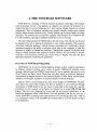
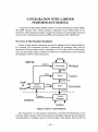
1. INTRODUCTION
In the late 1980s, the Federal Highway Administration (FHWA) assigned a high
priority to research and development of better highway design practices and criter:ia.The
goal of this multiyear program is to develop an interactive highway safety design model
(IHSDM) that systematically considers safety of roadway and roadside design elements
in creating cost-effective highway design alternatives. The computing environment is
intended to serve several purposes. First, it provides a data structure for the convenient
development of input and output data libraries. Second, it enables data to be shared
between the different modules of this computing environment. Third, it encourages the
integration of commercially developed and maintained vehicle dynamics, computer-aided
design (CAD) and finite element analysis (FEA) programs into FHWA's researlch and
design activities.
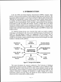
An integrated design process was conceived that would use modern computer
technology to simultaneously take into account significant factors of performance and
safety [ I ] . The road design is stored in a commercial CAD file format, such as
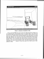
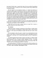
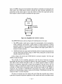
Intergraph's MICROSTATION or Autodesk's AUTOCAD. As shown in Figure 1, other
modules are envisioned to analyze proposed designs and provide the designer witlh rapid
feedback to identify possible problems.
Design
Alternatives
Benefit-Cost
Module
Consistency
Module
Policy Review /
Module
Accident Predictive
Module
i
Commercial
CAD Package
Roadside Safety
Structure Module!
Vehicle Dynamics
Module
Driver Performanc:e
Module
Revised
Alternatives
Traffic
Module
Figure 1. Concept of the IHSDM.
This report documents the research conducted at The University of Michigan
Transportation Research Institute (UMTRI) under FHWA Contract DTFH 61-93-R00142. The objectives of the research were to select vehicle dynamics models and link
them through a common database to standard commercial roadway CAD programs. The
software architecture is designed for flexibility to enable linking with a driver
performance model in the near future. The design also allows integration wit11 finite
element and other commercially available modules.
Project Deliverables
The project involved the following deliverables (in addition to this report):
The main deliverable is a comprehensive software package called VDM RoAD
(Vehicle Dynamic Models Roadway Analysis and Design). VDM RoAD was
developed to simulate the vehicle dynamics behavior of cars, trucks, and two-unit
combination vehicles (tractor-semitrailers) on 3D road designs. This software runs
under Windows 95 and Windows NT.
A full description of VDM RoAD, along with instructions for its use, is provided
in a 350-page reference manual, "VDM RoAD User Reference Manual Version
1.07,[21.
Two copies of the commercial simulation program TruckSim were delivered.
TruckSim supports vehicle dynamics studies that focus more on the vehicle and
less on the road design properties.
Two HP workstations were purchased for the project. One was shipped to the
Turner-Fairbank Highway Research Center in May 1995 and the other has been
used at UMTRT, as an Internet server for road profiles and public-domain software
maintained by UMTRI.
UMTRI prepared presentations, software demonstrations, and an exhibit for the
TRB-FHWA "3D Transportation Visualization and Simulation Symposium
Workshop" that was held in Houston during May 1995.
A UNIX program called RAPID COMBINE was created and delivered in 1995 to
combine vehicle response properties with road design data and speeds.
A UNIX version of the VDM RoAD was created. However, the UNIX version is
less developed than the Windows version.
Organization of this Report
This report is intended to describe the project for which VDM RoAD was developed.
The full documentation for VDM RoAD is provided in the user reference manual, "VDM
RoAD User Reference Manual Version 1.0" [2]. Section 2 describes the VDM RoAD
software. It has example applications and a short overview of the architecture. Section 3
covers the topic of how the vehicle dynamics models are integrated with road design
data. Section 4 discusses how VDM RoAD can be integrated in the future with the driver
performance module currently in development. Section 5 presents conclusions and
recommendations for future integration of vehicle dynamics models within IHDSM.
An appendix is provided that discusses the topic of lateral acceleration. During the
project it became apparent that some users were expecting the vehicle dynamics module
to predict lateral acceleration. This appendix was prepared to explain why lateral
acceleration is largely unrelated to vehicle dynamics.
2. THE VDM ROAD SOFTWARE
VDM RoAD is a marriage of vehicle dynamics simulation technology with roadway
CAD technology. In just a few minutes, an engineer can simulate the behavior of a
vehicle driving over several kilometers of a new roadway design. Results are viewed
immediately. Plots of important variables can instantly identify trouble spots (station
number) where excessive motions occur. Vehicle motions can be viewed with wire.-frame
animation. The software runs on Intel PCs equipped with Windows 95 or Windows NT.
It is self-contained, requiring no additional programs or tools to function.
The most striking feature of VDM RoAD is the ease of use. The software can be used
by engineers who are no experts in simulation or even vehicle dynamics. This colntrasts
with older simulation packages. Vehicle dynamics programs have traditionally offered
mechanical engineers the ability to perform virtual tests on the computer to study the
dynamics of vehicles in limited test conditions. Considerable expertise was needecl in the
fields of vehicle dynamics and numerical analysis. Further, the time needed to blecome
proficient with simulation software has always been so lengthy that only the most
determined engineers would become productive.
Overview of VDM RoAD Operation
VDM RoAD can be used to evaluate highway designs, as they would be experienced
by different vehicles traveling over a variety of speeds. VDM RoAD includes twelve
example vehicles from the AASHTO Green Book [3].It also includes data sets for a car
(Ford Taurus) and hexvy truck. Those data sets were based on extensive laboratory
measurements to support research at the National Highway Traffic Safety Administration
(NHTSA) involving the validation of computer models of vehicle dynamics.
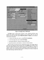
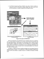
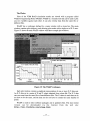
Figure 2 shows a screen dump of the main screen display in VDM RoAD. The pulldown menu lists some of the example runs that are installed. A user can browse through
the database of VDM RoAD or use the menu to jump right to the results for a specific
simulation run. For example, in the figure, the selected run is named WB-12 (Alt 3 R
Lane). This title was composed by a user and has not special significance to the
simulation programs within VDM RoAD. (The title indicates that the run invcllves a
vehicle called WB-12 running in the right-hand lane of a road design called Alt 3. \YB-12
is a combination vehicle in the AASHTO Green Book made of a 12-foot tractor towing a
12-ft semitrailer.)
Figure 2. Example runs in VDM ROAD.
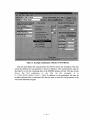
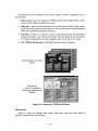
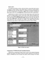
The Runs screen is shown again in Figure 3 with a different pull-down menu
showing. The window contains three categories of user controls: inputs, the run, and
outputs. On the left, under the caption Model Parameters & Inputs, are four links to
various kinds of input data:
1. a vehicle (in the figure the vehicle is called WB-12 Combination),
2. a road (in the figure the road is called Alt 3 Design),
3. target speed (defined as a function of station number), and
4. target lateral position (also defined as a function of station number).
These four links are made by the user with pull-down menus. For example, Figure 3
shows the screen appearance when the button next to the Vehicles link is clicked. A pulldown menu appears listing all of the vehicle data sets that are available in a "library" of
vehicles. In this case, the library contains combination vehicles involving trailers. A
different vehicle can be selected from the library by clicking on the button to display the
menu, then choosing a vehicle from the menu.
Figure 3. Example combination vehicles in VDM ROAD.
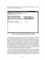
The next link defines the road geometry that will be used in the simulation. The data
screen that defines the road geometry is shown in Figure 4. The road geometric data are
described in a text file containing data in the IHSDM database format. The data screen
shows the full pathname to the file (in the example, it is
D : \VDM-ROAD \ROADS\ALT3 . IHM). In addition to the pathname, the data set
includes optional links to animation files that are used to draw the road geometry in the
wire-frame animator program.
Chain Name: ALT3
I n i t i a l Headin
S t a r t S t a t i o n : Ot000 End S t a t i o n : l t 9 5 0
Z
Radius
DAngle
0.00000
47.740
0.00
54156.295 117320.990
41.029
0.00
0.00000
54376.719 117196.281
40.377
0.00
0.00000
54398.111 117184.177
54402.657 117181.605
40.239 1 5 5 . 0 0 -44.50016
0.00
54420.596 117172.928
3 9 . 7 0 4 1 5 5 . 0 0 -44.50016
3 9 . 4 7 2 1 5 5 . 0 0 -44.50016
54429.842 117169.506
39.059 155.00 -44.50016
54489.751 117161.885
0.00000
39.298
0.00
54519.100 117166.792
0.00000
39.862
0.00
54587.192 117185.038
umber Regions: 1
0.000
253.257
277.836
283.059
303.260
312.861
373.641
403.443
473.938
70.00
Figure 4. Road geometry.
Another simulation input is a speed for the vehicle. As shown in Figure 5, the speed is
not necessarily a constant. The user can specify speed as a function of station number.
To make a simulation run in VDM RoAD, the user picks a vehicle, speed, and road,
using the links in the left region of the Runs screen. The controls and settings used to run
the simulation are in the middle of the screen (see Figure 2). There are fields for entering
a starting and stopping station number. For the example run represented in Figure 2, the
vehicle is initially located at station 0 and the run ends when the vehicle reaches station
1900. A button with the caption Run Simulation is used to make the virtual test on the
computer, simulating the specified vehicle running down the specified road under the
conditions defined by the links on the screen.
The mathematical vehicle models in VDM RoAD involve detailed nonlinear tire
models and nonlinear spring models. They include the major kinematic and compliance
effects in the suspensions and steering systems in cars and heavy trucks. The lunematical
and dynarnical equations are valid for full nonlinear 3D motions of rigid bodies. VDM
RoAD uses closed-loop controller algorithms to steer the vehicle along the specified path
and to drive at the prescribed speed.
The simulations run quickly, given the level of detail in the models. On Pentium-Pro
computers, the programs run in real time or faster. In other words, a run simulating a twominute test will finish in less than two minutes.
Figure 5. Target vehicle speed.
After a run has been made, the results are viewed using controls located in the righthand portion of the screen (see Figure 3). For example, clicking the Animate 'button
brings up an animation of the run, as shown in Figure 6. From within the animator, the
user can view the vehicle behavior in real time. A slider control (lower-left part of screen)
can be used to rapidly jump to any point in time. Other controls allow the user to change
point of view, zoom in and out, and advance in slow motion.
Figure 6. Animation of simulation results.
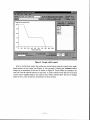
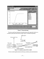
The user clicks the Plot button (also located in the right-hand portion of Figure 3) to
view engineering plots of the simulation results. For example, Figure 7 shows four plots
made this way. The upper-left plot shows lateral acceleration experienced by the tractor
and trailer, along with the lateral acceleration defined by the road geometry and vehicle
speed. (See Appendix A for a discussion of the lateral acceleration due to the road). The
upper-right plot shows the steering wheel angle needed to navigate the road with the
specified vehicle, speed, and lateral position. The plot underneath (lower-right) shows the
tracking of each wheel in the simulated vehicle. This plot summarizes the tracking
requirements for the combination of vehicle and speed for the entire section of road
(station 0 to 1900).
Figure 7. Example plots of simulation results.
Figure 8 shows four more plots from the same run. Here are plots of the vertical tire
forces and the vehicle roll angles for the tractor and semitrailer. Vehicle speed is also
shown, overlaid with the target speed, shown earlier as an input in Figure 5.
VDM ROADincludes more than 30 predefined plot setups such as the eight shown in
Figure 7 and Figure 8. Further, users can define new plots involving any combina~:ionof
the hundred or so variables stored on disk whenever a simulation is run.
1
Fz -- uert b c e s (RMe) vs 6 WB-12 (Ma Rlane)
'Meel had. N
Rwheel, axk 1
R wheel, axle 2
Rwheel axk3
R wheel, axle 4
.-
Fz nefl faces (L M e ) vsS WB-12 (A! 3 R lane)
11 Wlesl had. N
ii$ Lcndlxi~nalneloctl .b h
Vx us Men W.12 (At3 Rlane)
i
- L wheel, axls 1
t Lwhsel, & 2
* L wheel, axle 3
- L wheel, axle 4
I0
Figure 8. More plots for a simulation run.
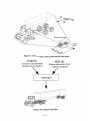
Software Architecture
VDM RoAD is made up of four tightly integrated types of software that are shown
conceptually in Figure 9.
1. Data screens serve as the primary interface to VDM RoAD. They contain vehicle
model parameters, control inputs, run settings, and links to IHSDM files with road
geometric data. The data screens are part of a database with many libraries of
related data sets.
2. Simulation programs numerically solve equations of motion (i.e., mathematical
vehicle models) to calculate output variables. The process of performing these
calculations is called making a simulation run. These programs are applied
automatically from the data screens when you click a "run button."
3. An animator shows the computed vehicle motions using wire-frame shapes for the
vehicle and road. The user can view the simulated motions, zoom in and out with
a virtual camera, and interactively move around the simulated vehicle to change
point of view.
4. The Windows Engineering Plotter (WinEP) creates plots of vehicle varialbles as
functions of time or as cross plots of output variables. This tool is used to view
any of the hundreds of variables computed by the simulation models.
Figure 9. Four parts of VDM RoAD.
Most user interactions with VDM RoAD involve preparing data sets for simulation
runs or viewing outputs of simulation runs. In either case, the user deals extensively with
the VDM RoAD database. The database was programmed using a software package
called ToolBook, available from Asymetrix, Inc. [4]. ToolBook is an scriptable objectbased software development tool primarily used for preparing educational and
multimedia material. It is also commonly used for prototyping graphical user interfaces
for complex software projects.
In addition to VDM RoAD, other simulation packages have been prepared using the
architecture shown in Figure 9. The architecture is called the simulation graphical user
interface (SGUI) and includes a standard extension to ToolBook developed at UMTRI
[5,61.
The database can be considered at four levels. Figure 10 shows a graphical view of
the first three.
1. Data screens. Any screen display in VDM RoAD that has editable fields or other
forms of user settings is called a data screen.
2. Data sets. A data set is the information you provide and can edit in a data screen,
minus the screen itself. The data screen is a view of a data set as seen through the
SGUI (the VDM RoAD graphical interface).
3. Libraries. A library is a collection of one or more data sets, plus the information
needed to provide a view in the user interface. The next figure shows the contents
of a library: multiple data sets, plus a graphical view of one data set at a time.
4. The VDM RoAD database. VDM RoAD includes about 50 libraries.
Individual data sets in the
library
Data Screen:
A view of one data set
though the graphical user
interface
Figure 10. Contents of a VDM RoAD library.
Data Screens
Figure 11 shows an example data screen. Each data screen has three kinds of
elements with which the user interacts.
1 . Yellow fields. These contain data that can be edited directly. For exarnlple, to
change wheelbase, find the yellow field with the current wheelbase value @,
click on the field, and change the value using the mouse and keyboard.
2. Buttons. All of the library screens include buttons at the top to quickly navigate
through the data sets in the library and to go to other libraries and programs in
VDM RoAD (see the buttons near
a).
H,
3. Pull-down menus. Some of the buttons are marked with a triangle
indicating
that pressing them with the left mouse button brings up a pull-down menu.
The yellow field in the upper-left corner of the screen is the title of the data set:
AASHTO 3-Axle Tractor @. (The title is simply text chosen by the user to identiify this
data set in the library. It has no significance to the simulation.)
Figure 11. Example data screen.
The Simulation Solver Programs
VDM RoAD contains programs that solve the equations of motion for vehicle
models, predicting motions, forces, and other variables. The solver programs a.re socalled console applications. Each behaves as a terminal console, with no user interface
other than the display of text and the acceptance of keyboard entries. Figure 12 shows
that they have the same appearance as a plain DOS text program. However, the solvers
are technically 32-bit Windows programs.
e n e r a t e d by AutoSim June 27, 1 9 9 7
I
S i m f i l e found: b a t c h o p e r a t i o n .
' I n p u t f i1 e w i t h parameter v a l u e s :
Echo f i l e w i t h i n i t i a l c o n d i t i o n s :
'Echo f i l e w i t h f i n a l c o n d i t i o n s :
u t p u t f i1 e w i t h t i m e - h i s t o r y d a t a :
u t p u t f i1 e w i t h l o g o f n e s t e d i n p u t s :
I........
C:\TRUCKSIH.INjRUNS\492.LPI
C:\TRUCKSIH.IN\RUNS~492.LP0
C:\TRUCKSIH.IN\RUNS\492.LPF
C:\TRUCKSIH.IN\RUNS\492.ERD
C:jTRUCKSIH.INjRUNS\492.LOG
....................................
r o g r e s s ( p e r c e n t complete] :
50
PC=31=E=====3===='=================
Figure 12. Screen display when solver program is running.
The solver programs contain equations of motion for the vehicle model in the form or
ordinary differential equations. The equations are far too complex to solve in closedform, so numerical integration is used. The source code for each simulation program is
generated using the AutoSim commercial multibody program [q.All of the equations
related to the kinematics and dynamics of rigid bodies are derived and assembled
automatically. However, equations for the tires, spring, driver model, and road geometry
are contained in hand-written subroutines that are linked with the AutoSim-generated
code. This approach allows highly complex mechanical systems to be simulated with
high confidence that most of the computer source code is free of common human errors.
Also, the equations generated by AutoSim have been shown to be highly efficient,
generally running faster than equations generated by other means [8].
When a simulation program runs, it creates summary files that list each parameter
value. One of these files is created before the run (LPO), and the other is created at the
end of the run (LPF). Both contain all parameter values. In addition, the LPO file
contains the initial conditions for the state variables in the simulation. The information in
the LPO file is sufficient to exactly repeat a run. The LPF file is nearly identical, except
that instead of initial values, it contains final values of the state variables. By modifying
the start and stop times, an existing run can be continued, possibly using a different kind
of simulation program.
The main purpose of each simulation program is to calculate time histoiries of
variables of interest. Those time histories are stored in a binary data file wiith the
extension BIN. The BIN files contain numerical data organized by channel number and
sample number, similar to test data recorded on a multitrack recorder. A companion file,
with extension ERD, describes the layout of the BIN file and contains labeling
information for each variable. It also contains the information that would normally be put
into a log sheet summarizing the data, including text needed for preparing graphical1 plots
of the data. By convention, ERD and BIN file pairs are simply called ERD files. The
name ERD is used because the format was created by the Engineering Research Division
at UMTRI, where it has been used since the early 1980s.
Data processing programs for ERD files obtain most of the information needed from
the file itself. For example, the high level of automation in the animator and plotter exists
because both were designed to work with ERD files.
VDM RoAD can also be made to produce simple text output files, for export to
spreadsheet programs and other analysis software.
The Animator
VDM RoAD includes a program for animating wire-frame figures to visualize vehicle
motions. The animation is accomplished by drawing images similar to what woilld be
seen with a video camera and updating the images many times per second to show
motion.
The view depends on where the camera is located. It is also determined by how the
camera is aimed. Figure 13 shows the basic geometry and the relationships between the
camera point, a look point, the 3D system being animated, and the 2D image that is
recorded.
The animator program reads two kinds of input files (see Figure 14). Motion variables
are read from an ERD file, created by the simulation programs whenever a run is ;made.
Other information-such as program settings, definitions of parts, and ;shape
information- are described with keyword-based text files (with extension PAR). The
PAR files transfer user settings from the SGUI to the animator.
The animator program in VDM RoAD is also used in other software packages imd is
updated often. The most recent version can be downloaded via the Internet from the web
site: httg ://www. trucksim. com/animator html.
.
Figure 13. Geometry of the camera point and the look point.
PAR files
ERD file
Animator set up and shape
information from database
Motion information from
simulation programs
/
Animator
Figure 14. Animator input files.
The Plotter
Plots of the VDM ROAD simulation results are viewed with a program called
Windows Engineering Plotter (WinEP). WinEP is a versatile tool that can be used to plot
any two variables against each other. It can also overlay data from the same file or
different files.
WinEP has a workspace defined by a main window with a menu bar. The main
window contains plot windows, each showing plots made with a single set of X-Y axes.
Figure 15 shows the main WinEP window with three example plot windows.
Tractor
Road
Semtailer
Y vs X -- trajectory : WB-20 (Alt 3 R lane)
Y pos'ilion m
117400
-
117200
117000
116800
54000
55000
X coordinate - m
150
200
250
300 350 400
W o n number m
-
450
500
550
Figure 15. The WinEP workspace.
Each plot window contains a graphical representation of one or more X-Y data sets.
An X-Y data set is a series of X and Y values obtained from a data file. The X-'Y data
sets can come from the same file or from different files. The X values in each data set do
not have to be the same, and the data sets do not have to contain the same number of
points.
WinEP is used in other software packages and is updated often. The most recent
version can be downloaded via the Internet from the web site:
http://www.trucksim.com/winep.html.
II
Batch Control
The VDM RoAD database includes vehicle descriptions, target paths (lateral position
as a function of station number), target speeds (speed as a function of station number),
and IHSDM data files with road geometry. The database also includes descriptions of
runs, plots, and animations. For example, the Runs screen (see Figure 2 and Figure 3)
shows a data set for a run, and the Runs library contains the data sets for numerous runs.
VDM RoAD also contains several data sets that include groups of runs and/or plot
settings. For example, Figure 16 shows a screen used to make a batch of simulation runs.
The user uses the Add and Remove buttons to create a list of runs in the lower-left part
of the screen (under the heading Data Sets to Run). Each line in this list is the name of a
data set from a Runs library. After the list is created, the user can update all runs with a
single button click. This is convenient, for example, if the roadway design has been
changed and a large number of vehicle responses are of interest for the new design.
Figure 16. Batch run control.
Comparison of VDM RoAD and TruckSim Features
VDM RoAD uses mathematical models similar to those in the commercial programs
TruckSim and CarSim. The models are based on research conducted over the past few
decades at UMTRI [9,10]. The TruckSim and CarSim software packages were further
developed and commercialized by Mechanical Simulation Corporation (MSC), a private
company in Ann Arbor, Michigan. MSC licenses, maintains, and supports TnlckSim and
CarSim.
TruckSim and VDM ROAD use the same graphical interface and database, thle same
animation program, and the same plotter. The vehicle models have the same: input
parameters, and the same equations are used to simulate vehicle dynamics. However,
TruckSim is designed for mechanical engineers interested in studying vehicle dyiiamics
and the effects of changes in vehicle design. On the other hand, VDM RoAD is designed
for civil engineers to evaluate candidate road designs and to see the effect of changes in
road design. Accordingly, the two software packages have some significant differences,
as summarized in Table 1.
In order to make new runs with TruckSim or CarSim, the user must have a hairdware
"key" (called a DONGLE) that attaches to the parallel port of the PC. FHWA ha.s been
provided with two copies of TruckSim, along with two hardware keys.
All rights to VDM RoAD have been transferred to the government. The VDM RoAD
software does not require a hardware key and can be distributed as the government
chooses. The source code for VDM RoAD has been provided to FHWA.
Table 1. Comparison of TruckSim and VDM RoAD features.
Vehicle Model Features
Full nonlinear 3D equation sets
Full nonlinear suspension components
Nonlinear brakes with air dynamics and ABS
Full nonlinear tire model with 2D tables
Alternate support for ST1 tire model (1994
version)
Full 3D tirelroad interface (slope + cross slope)
Number of truck models
Number of car models
Unit systems
Control and Road Inputs
UMTRI driver model for following path
Speed control
Open-loop steer control
Brake input
IHSDM interchange file
User-specified initial conditions
User-specified road friction
Simulation stopping variables
Vehicle X-Y-Z and yaw-pitch-roll for animation
Lateral accelerations
Tire forces and moments
Slope and cross slope under wheels
S, L coordinates of wheels
Road-based points-of-view for animator
Tire kinematics: lateral slip, inclination, etc.
Suspension spring and damper forces and
deflections
VDM RoAD
TruckSim
Yes
Yes
Yes
Yes
Yes
Yes
Yes
Yes
Yes
No
Yes
4
1
metric
No
6
0
metric or
English
L vs. S
V vs. S
No
Pressure vs. T
Yes
s,L
Yes
S, T, Roll, V
Y vs. X
V vs. T
Steer vs. T
Pressure vs. T
No
XYZ, angles
Yes
T, Roll, V
Yes
Vehicle, road
Yes
Yes
Yes
Yes
No
No
Yes
Vehicle
Yes
No
No
No
Yes
Yes
3. INTEGRATION WITH ROAD DESIGN DATA
This section provides an overview of the road geometry used in the VDM RoAD
models, and then describes how the road design data are integrated with the vehicle
dynamics models.
The road design data are used to perform several functions in the VDM RoAD
design:
1. to provide a continuous 3D surface that supports the vehicle and interacts with the
tires,
2. to provide a horizontal path as a reference for the closed-loop steering mode:l, and
3. to determine the location and orientation of the vehicle at the start of a simulation
run. (The location and orientation are part of the vehicle "initial conditions.")
Using road design data together with a vehicle dynamics model requires the
information in the roadway coordinate system to be compatible with the vehicle
coordinate system. The following subsections describe the roadway and vehicle
coordinate systems, and the general methods used to transform information between
them. After the roadway coordinate system has been described, the section concludes by
describing how the above three functions are accomplished.
Coordinate Systems
The describing dynamical equations for a vehicle are solved by the sirnullation
programs in VDM RoAD to provide coordinates of critical points in the vehicle ba;sed on
a global X-Y-Z coordinate system. The road design data from the IHSDM data file is also
tied to a global X-Y-Z coordinate system. The global system is needed by the underlying
CAD system to perform calculations and to prepare graphic views of the design.
The location of an arbitrary point P in 3D space requires a coordinate system with
three independent coordinates. For the X-Y-Z system, the three coordinates are X, Y, and
2--each defined as the distance from the origin along a line parallel with the named axis.
To locate point P, one would:
1. start at the origin and then go X meters along the X axis,
2. then go Y meters parallel with the Y axis, and, finally,
3. go Z meters up, parallel with the Z axis.
The global X-Y-Z coordinate system is theoretically sufficient for locating any point
of interest in the road and any point of interest in the vehicle at a specific instant of' time.
However, it is desirable to locate the vehicle using station number (S) and lateral distance
(L) from the design centerline, rather than global X and Y coordinates.
The data in the IHSDM file define a continuous, curved reference design line
(typically the centerline) in 3D space. The 2D horizontal geometry is defined by
projecting the 3D line onto the global X-Y plane, as shown in Figure 17. Station number
is defined as the distance along the 2D projection.
Figure 17. The S-L-Z coordinate system.
The road coordinate system in VDM RoAD involves three coordinates named S, L,
and Z. The Z coordinate is the same as in the X-Y-Z system. The other coordinates, S and
L, are based on the design centerline. To locate point P in the road coordinate system, one
would:
1. start on the projection of the road design line into the X-Y plane at station S=O
and then travel along the projection of the design line S meters,
2. then go laterally L meters, along a line in the X-Y plane that is perpendicular to
the projection of the design line, and finally,
3. go up Z meters, parallel with the Z axis.
The right-hand rule requires that L be positive for positions to the right of the
centerline when facing "upstream" (in the direction of decreasing S). If facing in the
direction of increasing S, then points to the left of the centerline are positive and points to
the right are negative.
The sign-convention for L defines a "right-handed coordinate system" when positive
Z is up. Only right-handed coordinate systems are used in complex commercial 3D
software packages. Thus, a right-handed system was defined for VDM RoAD.
Coordinate System Transformations
The Z coordinates from the X-Y-Z and S-L-Z systems are the same. Therefore,
transformations between the two systems involve only the two-dimensional X-Y and S-L
systems.
The process of transforming S-L coordinates into X-Y values is direct. For any ]pair of
S-L values, there is a single pair of X-Y coordinates. Figure 18 shows the geometry for
an arbitrary point (X, Y), the centerline, and a design point on the centerline (Xi, Y,).
Centerline
Figure 18. Computation of X-Y from S-L.
The process for computing X and Y is as follows:
1. Find the index i for the last design point preceding S. This is done using a tablelookup procedure.
2. Compute the S distance of the current point past the last design point. This change
is shown in Figure 18 as AS.
3. Compute changes in X and Y in a rotated coordinate system where X is tangent to
the centerline at the design point. These changes are shown as AXs' and b'Y,' in
Figure 18. The details of the calculation depend on whether the road centerlline is
(a) straight, (b) has a constant radius, or (c) is on a spiral.
4. Using the heading angle of the centerline at the design point, transform the
quantities AX,' and AYs' to obtain X and Y changes in the global coordinate
system (AXs and AYS).
5. Add AX, and AYs to the coordinates of the design point, XI and Y,. This givles the
X and Y coordinates at a point on the design centerline at S.
6. Determine the heading angle at S. (Different methods are used depending on
whether the road is straight, on a constant-radius turn, or on a spiral.) Use the
heading angle to determine changes in X and Y due to L.
7. Add the X and Y offsets (from step 6) to determine the X and Y coordinates for
the point at S, L.
Additional details of the transformation are provided in Appendix H of the VDM
RoAD User Manual [ 2 ] .
Converting from X-Y coordinates to determine S-L values is not as direct as the
above transformation. One complication is that multiple values of S-L can exist for a
single point in X-Y space. For example, the center of a design curve can be equally well
defined using any value of S along the curve, with the magnitude of the L value being
equal to the radius.
The method is described in Appendix H of the user manual. It requires knowledge of
the design point Si that is associated with X and Y. Separate transforms are presented for
tangent and constant-radius turns. The geometry has not yet been worked out for spirals.
A procedure is followed to compute AS and L. The calculated value of AS is then
inspected, to see if the assumed design point was correct. For example, if the design point
is located at the start of a curve covering 200 meters, the valid range of AS is 0 to 200. If
the computed value of AS is greater than 200, then the calculated values of S and L are
not correct because the point of interest is past the end of the curve. In this case, the
procedure would be repeated using the next design point.
Applications of the Road Coordinate System
As noted at the start of this section, there are several applications of the
transformations in VDM RoAD.
TireIRoad Interactions
The most essential application of the road geometry is to define the 3D ground
surface under each wheel of the vehicle, such that the interactions between the ground
and the tires can be computed. Figure 19 shows vectors that describe the four main
actions on the vehicle generated by the tire: longitudinal force (F,), lateral force (F,),
vertical force (F,), and aligning moment (M,). The three forces apply at a point defined
by the intersection of the wheel plane with the 3D road surface. his point, labeled W, in
the figure, has X and Y coordinates that are known approximately from the vehicle
model. The Z coordinate is determined by the road design data.
Figure 19. Directions of tire action vectors.
The road normal vector is shown in the figure and labeled r,. (The road norrrial is a
vector whose direction is perpendicular to the road surface.) If the road is flat ancl level,
r, points straight up, in the direction opposite of the gravity vector. However, in general,
it is tilted slightly due to vertical geometry and superelevation. The road norrnal is used in
the vehicle dynamics models, together with the direction of the spin axis of the wheel, to
define the vectors t, and t, that define the directions in which the tire longitudin~aland
lateral forces are applied.
In order to calculate the directions of the vectors, it is necessary to determine the road
normal at each tire location (W,). Starting with the X and Y coordinates of point W,, the
vehicle simulation programs in VDM ROAD compute Z and two slope values. The
process is as follows:
1. Determine the S-L coordinates associated with the point by transforming the
known X-Y coordinates.
2. Determine the Z coordinate of the design centerline at S, based on vertical
geometry data. Also, determine the longitudinal slope: anas.
3. For the current station (S), calculate change in Z as a function of L due to design
superelevation. Also, determine the lateral slope: aZ/aL.
4. Add the superelevation effect (step 3) to the centerline elevation (step 2) to obtain
the total height of the road surface at the wheel contact point.
5. Transform the two slope values (aZ/aS and aZ/aL) to slopes with respect to the
global X and Y directions (aZ/aX and aZ/aY). Use the sine and cosine of the
road-heading angle to accomplish this.
The complete details for computing Z and the two slope quantities are presented in
Appendix H of the VDM RoAD Users Manual. The application of these quantities to the
vehicle model is described in Appendix G.
Interactions With the Closed-Loop Steer Controller
In order to simulate the driving of a vehicle over a 3D road design, the vehicle models
in VDM RoAD include a closed-loop steering controller. Figure 20 shows a simple flowchart of the controller logic.
target path
Full response
Full vehicle dynamics
simulation
Figure 20. Closed-loop steer controller.
The driver model takes as inputs a target path and some feedback variables from the
full vehicle model. The controller works by looking ahead by some amount of time and
determining the steering wheel angle (shown in the figure as u,) that will cause the
vehicle path to best match the target path over the preview interval. The steering from the
driver is added to a steering due to other factors (mechanical kinematic and compliance
properties of the suspension), shown in the figure as u,.
The driver model includes parameters, control logic, and even a simplified vehicle
dynamics model. The target path is defined with a table of L versus S values, as shown
for an example lane change in Figure 21. In the figure, the input path would start at the
design centerline, changing to a point 3.35 m left of the centerline after station S=135 m.
Figure 21. Target path input.
The driver model must determine the lateral position of the target path, relative to a
coordinate system based on the moving vehicle. Figure 22 illustrates the geometry.
/
Driver model Y axis
Inertial Y
1
(inertial coordinates)
Figure 22. Coordinate system of driver model.
The driver model algorithm makes the following coordinate system transformations:
1. The global coordinates of a reference point (X,, Y,) are converted to the roadway
S-L system to determine the station number for the reference point.
2. Using the current vehicle speed and direction (increasing station or decreasing
station), station numbers are computed for 10 equally spaced target points lying
ahead of the vehicle. The distance to the 10th target point is the preview time
(sec) multiplied by the current vehicle speed (mtsec).
3. At each of the 10 target points, the lateral coordinate of the target path (see Figure
21) is determined by table lookup.
4. The S-L coordinates for the 10 target points are transformed to the inertial X-Y
coordinate system.
5. The lateral location in the driver model coordinate system is calculated for each
target point by first getting the inertial X and Y coordinates of the path as
functions of the station at the target location (Stag), and then applying the
transformation
where w is the vehicle heading angle.
The above strategy is valid for any location of the vehicle where a station can be
computed. At zero speed, the look-ahead is set to a small distance to avoid numerical
problems. Complete details of the control algorithm are described in Appendix I of the
VDM RoAD Users Manual.
Initialization of the Vehicle Position
At the start of each simulation run, the vehicle position and orientation are set to
match the road geometry, initial station number, target speed, and target lateral position.
The user of VDM RoAD specifies a starting and stopping station number for each
simulation run. For example, in Figure 2 on page 4, the run starts at station 0 and stops at
station 1900. The starting and stopping station numbers are used for three purposes in
VDM RoAD:
6. The starting station number, designated So,is used to locate the vehicle at the start
of the run.
7. The stopping station number is used as a criterion for stopping the run.
8 . The starting and stopping station numbers are compared to determine the
direction the vehicle is traveling (increasing station or decreasing station).
More specifically, the initial conditions of the vehicle are set as follows:
r
The vehicle reference point (center of front axle) is located at the starting station
number So specified on the Runs screen.
The vehicle reference point is located at the lateral position L specified as the
target location at the given starting station: L(S,).
The heading of the vehicle is set to match the heading of the road at S,, when
vehicle is traveling in the direction of increasing station. When traveling in the
opposite direction the heading is set opposite that of the road.
The pitch angle of the vehicle is set to match the longitudinal slope of the :road at
So. When traveling in the opposite direction, the negative slope is used.
The roll angle of the vehicle is set to match the superelevation of the roald at So
and L(S,). When .traveling in the opposite direction the negative supereleva~tionis
used.
The tire deflections are set to provide the static loads that would be expecte:d on a
flat, level surface at zero speed.
Suspension deflections are set to provide the static spring forces that would be
expected on a flat, level surface at zero speed.
Forward vehicle speed is set to match the user-specified input: V(S,).
The tire and suspension deflections are generally not exactly equal to the equi1:ibrium
values, although they are close. For the car model, aerodynamic forces and momeilts are
neglected. For all models, a number of secondary effects are neglected. For example, load
transfer is neglected between wheels due to small pitch and roll angles. Consequently, the
first second or so of the simulation usually includes some bouncing, pitching, and irolling
of the vehicle as it settles into an equilibrium condition on the 3D road surface in the
presence of aerodynamic effects.
4. INTEGRATION WITH A DRIVER
PERFORMANCE MODULE
A major part of the planned IHSDM system is a driver performance module (DPM).
The DPM interacts with vehicle dynamics simulations from VDM RoAD (or an
alternative vehicle dynamics module) to predict the motions of a driverlvehicle system on
the road. This section describes how the DPM can be integrated with VDM RoAD.
Overview of Man-Machine Simulation
Models of man-machine interactions can involve multiple levels of human behavior.
For example, Jens Rasmussen provides a framework for providing three levels of
abstraction involving human control of machines [ I l l . The three levels are called skills,
rules, and knowledge. Figure 23 shows how these levels of performance can be related to
the modeling of driver-vehicle interactions.
Goals
DRIVER
Symbols
Knowledge
Strategy
Plans
Signs
Sight
&
Sound
Rules
Tactics
Skills
Execution
.IIIIIIIIII
Motion
SYSTEM
Vehicle
Dynamics
T
Action
1
Figure 23. Driver control behavior.
The "big picture" of man-machine interaction as described by Rasmussen covers
extremely abstract notions, such as the analysis of unfamiliar situations and development
of general plans or strategies, based on the knowledge of the human. The next level is
less abstract. It involves tactical decisions based on rules developed from past experience.
The outcome of the knowledge and rule-based behavior are commands. In the conltext of
the driver of a vehicle, the commands are a target speed and lateral position of the vehicle
on the roadway. The third level of behavior involves the driver controlling the vehicle
through the steering wheel, throttle, and brakes. The objective of the driver is to use
previously learned skills to execute the commands.
Integration of DPM and VDM
The DPM is presently in the early stages of development, and details of its opelration
have not been finalized. However, it is probably safe to assume that at least the two innerloops shown in Figure 23 will be included in the IHSDM (simulation of driver rulies for
choosing paths and speed, and simulation of driver steering and speed control).
There are several methods by which the DPM and VDM modules can be integrated.
Three possibilities are mentioned below.
1. The DPM and VDM programs can be merged into a single program that sim,ulates
both the vehicle dynamics and the driver control behavior.
2. The DPM and VDM programs can be modified to run concurrently, exchanging
information as they run.
3. The DPM and VDM programs can be run sequentially. The DPM would bt: used
to generate target paths and speed, and then the VDM program would be :run to
generate the vehicle-specific response to those commands.
Of these three methods, the third is recommended. Before describing how the DPM
and VDM would be run sequentially, the rationale will be presented for rejecting the first
two approaches.
Problems with Running DPM and VDM Simultaneously
Merging the DPM and VDM parts of IHSDM would invol've taking the computer
source code (C, Fortran, etc.) for the two modules and combining the code into one single
program module. Although this approach is conceptually simple, it is not practical. The
VDM RoAD simulation programs are large, complex programs that are designed as
"stand-alone" programs. They are not designed to be merged with other software and
there is no documentation that describes how this would be done. Considerable expertise
would be needed by the programmers to understand their design and modify them to
work together with the DPM.
It should also be noted that the vehicle simulation in VDM RoAD is not performed by
a single program. VDM RoAD includes five separate vehicle simulation programs each
customized with equations of motion for a specific class of vehicle (cars and four
configurations of heavy trucks). At least five separate VDMfDPM programs would have
to be constructed. (Of course, it is also theoretically possible to merge the five separate
VDM programs and then merge that program with the DPM code. This possibility is
discounted because it involves even more work and requires even more expertise.)
Modifying the VDM and DPM programs to run concurrently and exchange
information is more feasible, but is still not recommended. There are at least two
problems. One is that considerable expertise is still needed to modify the programs to
properly exchange information. The programmers would have to master the design of the
existing programs before they could modify them. The second problem involves
efficiency. When multiple programs are run concurrently, there can be a great deal of
overhead and inefficiency introduced, resulting in long run times.
UMTRI researchers have experience in how software can slow down when several
simulation programs are made to run concurrently. A software package called ArcSim
was developed to showcase simulation technologies developed under the U.S. Army
Automotive Research Center (ARC) headquartered at the University of Michigan (see the
web site: h t tg :I I arc engin. umich e d u l ) . ArcSim includes simulations of a
military tractor-semitrailer with a mathematical model similar to the ones in VDM
ROAD. The ArcSim program was modified and made to run concurrently with a separate
simulation program, integrated using the commercial simulation program SimuLink
(SimuLink is sold by The Mathworks, Inc., as an add-on to its MATLAB package). We
found that two programs that both ran quickly by themselves were slowed down
considerably when they were integrated. A run that would take less than a minute for
either program by itself took hours when the programs were connected.
.
.
The slowdown was due partly to different time scales associated with the models.
However, the more significant problem was that the interprocess communication was
extremely inefficient. The problems of interprocess communication are, in our view,
solvable. However, the amount of effort needed to solve the problem is not known. The
problem of having different time scales also applies to the one of integrating VDM and
DPM. The vehicle models include the high-frequency dynamics of subsystems that
require small integration time steps, on the order of 0.002 sec. Removing the highfrequency dynamics reduces the accuracy of the simulation and is not easily
accomplished. The DPM does not require such a small time step. Values of 0.01 to 0.1
sec are more typical.
Running DPM and VDM Sequentially
In viewing the control flow chart in Figure 23, consider the computation requirements
for the three loops. The outer loop (knowledge) is so abstract it might be beyond the
scope of DPM. Abstract thinking does not involve rapid coupling with vehicle dynamics,
because the thinking process generally covers a time scale involving minutes or hours.
The intermediate loop (rules) is probably the main part of the DPM. Taking into account
traffic conditions, perceived road geometry, and the current speed and location of the
driver's vehicle, the driver model generates commands in the form of a target path and
target speed. The time scale involves seconds. The inner loop (skills) involves the close
coupling of the driver control and the vehicle response. Given a target path and target
speed, this level of control determines how the driver controls the throttle, brakes, and
steering wheel to achieve the targets. This time scale covers tenths of seconds.
Given that only the inner loop (skills) involves a short time scale (high frequencies),
it is possible to separate the driver control into two parts as shown in Figure 24. In this
figure, the DPM is the part of the simulation that produces commands: the target path and
target speed. The VDM RoAD software includes the skill controller algorith~msfor
generating steering wheel angle to cause the vehicle to follow the target path a.nd the
drive torque to cause the vehicle to maintain the target speed.
Path Command,
Speed Command
VDM RoAD
1
I
Action
7
Figure 24. Simplified view of driver control.
The DPMNDM system shown in Figure 24 would function in two steps:
1. The DPM module would take as inputs the road geometry, driver parameters,
traffic conditions, and possibly a small number of vehicle parameters. (V~ehicle
parameters might not even be needed.) As output it would produce the targe.t path
(lateral position as a function of station number) and target speed (also as a
function of station number).
2. VDM RoAD takes the target speed and lateral position as inputs and generates the
steering wheel angle and drive torque to follow them, taking into account the full
dynamic response of the vehicle.
In this design, the second part (VDM RoAD) is already complete. The first part
(DPM) is being developed.
The rationale for this modeling approach is that the driver behavior involving
knowledge and rules does not depend on details of the vehicle dynamics. It is assumed
that when a driver decides what path to take, it is without regard to details of vehicle
behavior. In planning a target path or speed, the assumption is that the driver will "do
whatever it takes" to control the vehicle to hit the target. If the vehicle is sluggish, the
controller in VDM RoAD will generate larger steering wheel angles. If the vehicle is
responsive, the controller in VDM RoAD will generate less control. The DPM can
perform all of the planning without concern for the details. VDM RoAD will then "do
whatever it takes" to execute the plans.
Of course, in extreme cases, the vehicle will crash. When the controller tries to follow
a path that is beyond the physical capabilities of the vehicle and road, an accident occurs
in the form of a rollover or of the vehicle skidding off of the road. In these cases, the
simulated driver behavior will be wrong, pure and simple. However, this limit in
accuracy is not necessarily a limit in the usefulness of the software. The basic objective is
to identify potential problems involving road design, vehicle type, driver behavior, and
signing. If the simulation shows a large amount of corrective steering, or tire loads
reaching zero, then a problem has been identified and the software has provided useful
information.
The details of how a driver and vehicle interact after the problem occurs is not of
interest if an alternative design can be developed.
5. CONCLUSIONS AND RECOMMENDATIONS
This section presents the main conclusions drawn from the project and presents
specific recommendations for the continued development of the IHSDM.
VDM RoAD Software
The main objective of this project was to select among existing vehicle dynamics
simulation programs and link them through a common database to commercial roadway
CAD programs. The existing TruckSim and AutoSim technologies were selected and
extended for this project. The connection to roadway CAD packages is made through a
standard IHSDM interchange file that is created as an output by CAD packages such as
GEOPAK and read as an input by VDM RoAD.
The VDM RoAD provides an advanced simulation of vehicle dynamics that works
with the 3D road design data. In just a few minutes, an engineer can simulate the
behavior of a vehicle driving over several kilometers of a new roadway design. R.esults
are viewed immediately. Vehicle motions can be viewed with wire-frame animation.
The software can be used by engineers who are not experts in simulation or even
vehicle dynamics. This contrasts with older simulation packages where considerable
expertise was needed in the fields of vehicle dynamics and numerical analysis. Further,
the time needed to become proficient with simulation software has always been so
lengthy that only the most determined engineers would become productive.
The software runs on Intel PCs equipped with Windows 95 or Windows NT. With
Pentium Pro or Pentium I1 machines, the simulations run faster than real time.
The new software is almost ideal for simulating what would happen if a particular
vehicle is operated on a particular road with a given input path (lane positionl as a
function of station number) and speed (also specified as a function of station number).
We recommend that the software be used for this purpose.
The UNIX Platform
When this project started in late 1993 the vehicle models and supporting programs
existed only on the Windows platform. Yet, most States with road design CAD systems
were using UNIX. As the project developed, one of the contract modifications included a
task of porting the software from Windows to UNIX. A partially functional version of
VDM RoAD exists on UNIX:
The simulation solver programs are generally platform independent. The code is
written in Fortran 77 and runs on any machine with a suitable compiler. Most of
the code also exists in C (the exception is the interface with the IHSDM
interchange files). There were no problems generating executable binary UNIX
files.
r
The plotter and animator are C programs that make use of the graphics and user
interface libraries of specific operating systems. The Windows versions make use
of well-developed libraries and development tools that only exist for Windows.
The UNIX versions are functional but would require considerably more
development effort to reach the same level of utility as the Windows versions.
Performance of the animator was disappointing-it runs slower on a workstation
than the Windows version on a low-end PC.
r
The graphical user interface on Windows is programmed in ToolBook [ 4 ] . A
similar product for UNIX exists that is called MetaCard. However, we found that
our productivity with MetaCard was much less than with ToolBook. We were
never able to program the same level of functionality in the UNIX version of the
graphic interface as was possible in the Windows version. We are not sure it is
even possible.
Before the project concluded, FHWA changed the platform of choice for IHSDM
from UNIX to Windows/NT.
We recommend that all UNIX products developed in this program be abandoned.
If there is a need in the future to run the vehicle dynamics simulations under UNIX,
the source code for the vehicle models can be easily compiled. However, we would not
recommend attempting to reproduce the other parts of VDM RoAD unless improved
development tools become available.
Integration with Road Design Data
In its current version, VDM RoAD is integrated with IHSDM through the interchange
file format that summarizes the entire 3D road geometry. A portion of an interchange file
is shown in Figure 4 on page 6. The road design data are presented in tabular form with
37 columns. Each row in the table represents a change in some property of the design.
For example, a new row is needed at the beginning or end of a turn to specify properties
of the new radius, spiral, or tangent. A new row is also needed at any transition in the
vertical geometry or any transition in the superelevation in any of up to 14 lanes.
The interchange file contains three kinds of design information:
1. horizontal geometry of the roadway centerline;
2. vertical geometry of the roadway centerline; and
3. transverse profile information (width and slope) for 13 sections (four lanes, parts
of the median, and parts of the outside ditches).
The file also contains redundant information (X-Y-Z coordinates and heading angle).
Because all three kinds of information are written in the same file, it is neces,sary to
put a row in the table for any station number where any of the three kinds of infonmation
start a transition.
There are two difficulties caused by this format. First, the large number of columns
(37) and the redundant information make the interchange file difficult to create by hand
for debugging and performing quick "what if' analyses. It is only practical to create the
files by computer, even though the information contained might be very simple. The
second problem is that the software reading the file must deal with extraneous rows of
data that are unrelated to the information of interest. For example, a program dealing only
with vertical geometry must read every row of data involving changes in horizontal
geometry or superelevation. The program must include logic to determine that those lines
from the input file are not: relevant and should be ignored.
The three kinds of design data are independent. Software that reads design data could
be programmed more efficiently if each kind of information were stored in a separate file.
Therefore, we recommend that a new interchange format be designed for future work.
The new format should use separate files to store horizontal geometry design data,
vertical geometry design data, and superelevation design data.
Integration of Vehicle and Driver Performance Models
Section 4 presented a framework for describing man-machine interactions at three
levels, based on (1) knowledge, (2) rules, and (3) skill. It is only in the third category
where rapid driver control (skill) interacts with the vehicle dynamics, such that the
vehicle is controlled as needed to follow commands in the form of target speeid and
lateral position (within the lanes of the roadway).
The part of the driver model that determines the target path and speed is largely
unaffected by details of the dynamic response of a specific vehicle. Therefore we
recommend that the DPM be developed using a simple point-mass representation of the
vehicle to determine the target speed and lateral position. (Perhaps the driver rnodel
would not even need a point mass. It might be that the target speed and path can be
determined based only on kinematical considerations, involving speed, point of view of
the road geometry, traffic, and environmental factors.)
VDM RoAD already includes the skill part of a driver model and can reald the
position and speed outputs generated by the DPM.
Use of Vehicle Dynamics Simulation in Roadway Design
The IHSDM project is an ambitious undertaking, and one in which the direction has
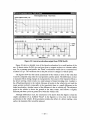
changed as progress is made. When this project started, an objective was to select the: best
existing vehicle dynamics models and integrate them into the IHSDM so they could be
used to run a fleet of vehicles over a candidate 3D roadway design. VDM RoAD was
developed and meets this objective. However, just because vehicle dynamics programs
can be used by designers does not mean they should be used.
When IHSDM was envisioned, it was thought that full simulation of vehicle
dynamics would be needed to evaluate the suitability of a road design for use by a variety
of vehicles. As a minimum, the fleet of simulated vehicles would match the 15 examples
from the AASHTO Green Book.
Upon considering the objectives of a designer, we do not recommend the continued
integration of VDM RoAD within IHSDM for improving the design process. We
conclude that the concerns of the designer are so specific that a more efficient approach
should be used. Some specific concerns that involve vehicle responses are:
1. Will the lateral acceleration experienced by drivers exceed limits found in the
AASHTO Green Book? (Those limits involve low levels of acceleration and
indicate a threshold of discomfort.)
2. Will any vehicles run into frictional limits and risk running off the road due to
skidding?
3. Will any vehicles risk rolling over?
4. Will large vehicles have difficulty navigating sharp turns due to offtracking?
5. Will hill climbing challenge underpowered vehicles to maintain high speed?
6. Will long descents challenge the ability of heavy trucks to maintain low speed?
We recommend that items 5 and 6 be predicted with a different type of model than
used in VDM RoAD. For hill climbing, a simple point-mass representation with a
parameter specifying the powerlweight ratio is sufficient. For hill descending, a thermal
model to predict brake temperature and fade would be needed.
The first four items can all be addressed with models much simpler than the ones in
VDM RoAD. Following are the recommendations for providing feedback to the designer
in IHSDM for these four items.
Lateral Acceleration (Comfort)
Lateral acceleration is defined solely by the geometry of a path taken and the instant
speed. The equation is:
where V is forward speed and R is the instant radius of the path. The radius is a
combination of the roadway geometry and the relative lateral position taken by the
vehicle within the road. The dynamic properties of the vehicle have only a minor effect at
transition points (see Appendix A for a more detailed discussion).
We recommend that equation 1 be used to compute lateral acceleration as a function
of the target speed generated by the DPM. A detailed vehicle model is of no use for this
purpose.
Vehicle Rollover
A vehicle navigating a turn is subject to centrifugal force acting on its center of mass
and causing the vehicle to roll away from the turn (e.g., the vehicle rolls to the right in a
turn to the left). If the vehicle rolls so much that the inner wheels lift off the ground, it is
unstable and rolls over. The propensity of vehicles to rollover is characterized by a
rollover threshold-the maximum lateral acceleration that can be sustained by the vehicle
before rollover occurs. Rollover threshold is measured experimentally with tilt tabl~esthat
simulate the effect of lateral acceleration. The rollover threshold can be obtained with
detailed vehicle simulation models such as those in VDM RoAD or TruckSim.
The rollover threshold of a vehicle is generally not considered to depend on the
geometry of a roadway. The assumption underlying a tilt table is that the threshold found
from the test is a valid indicator of the rollover stability under any condition.
A roadway designer should be concerned with the rollover threshold of the "worst
case" vehicle that will be allowed on the road. Given a rollover threshold, equatioln 4 in
Appendix A determines the maximum speed that should be allowed for a given raclius of
turn.
In general, rollover thresholds are above 0.35 g's for most heavy trucks, and above
0.25 g's for nearly all conventional highway vehicles. These levels are much highex than
the limits specified in the Green Book (about 0.1 g), which implies that the maximum
speed for rollover considerations will be higher than the design speed, assuming a
realistic worst-case rollover threshold.
We recommend that equation 4 be used to compute the maximum safe speed based on
a single worst-case rollover threshold. A detailed vehicle model adds little if any fuinction
for ordinary design evaluation.
Friction Utilization
Friction utilization is the ratio of tire shear force divided by the tire vertical force. As
long as the utilization is less than the available friction, the tire grips the road as expected
by the driver. The lateral acceleration predicted by equation 5 in Appendix A is
equivalent to friction utilization for the simplest possible vehicle model (a point mass).
Detailed vehicle models such as those in VDM RoAD give the friction utilization for
each tire and can provide more accuracy when the utilization is close to the frictional
limit.
The acceleration limits from the Green Book are much lower than friction levels
associated with sliding-about 0.1 g for highway speeds. This means that sliding will
only be a problem for travel speeds well above the limit associated with the Green Book
design guidelines.
Friction utilization is not going to be an issue for any highway vehicle :if the
acceleration limits from the Green Book are met. It is only possible to exceed the: road
friction by traveling at speeds much higher than the design speed. For design purposes, a
good predictor of the friction utilization is the lateral acceleration predicted by equaltion 5
in Appendix A. The equation can be manipulated to compute a maximum speed (V).
In general, the speed associated with a specification of friction utilization will be
higher than a speed associated with comfort or rollover.
We do not recommend the use of detailed models such as those in VDM RoAD as a
design tool involving friction utilization.
If a designer wishes to know the maximum speed possible before a specified level of
friction utilization is reached, we recommend that equation 5 from Appendix A be used
to compute the speed as a function of station number according to changes in design
radius.
Vehicle Offtracking
Highway vehicles with front-wheel steering systems have the characteristic that when
turning, the wheels of the rear axles track inboard from the paths followed by the front
wheels. This behavior is of concern when designing intersections, truck loading areas,
bus-stop areas, and any roadways or pavements where large vehicles must turn. The
vehicle models in VDM RoAD can be used to determine tracking requirements for any
geometry that is described using the IHSDM interchange file format. However, the
behavior can also be simulated using much simpler means. Decades ago, a drafting tool
called a tractrix integrator was used to draw the paths followed by the wheels of trucks
making sharp turns. Graphic templates are included in the AASHTO Green Book for the
15 design vehicles. The AASTHO templates are probably the most commonly used tool
for evaluating intersection designs.
In the 1980s FHWA supported the development of software on a personal computer
to perform the same function [12]. A simpler formulation was later published in which
the equations fit on a single page, even for combination vehicles such as double-trailer
vehicles [13].
As with other types of design criteria, we recommend that candidate designs be
evaluated only for the worst-case vehicle. For offtracking, this is usually a single unit
vehicle with the largest wheelbase allowed on the road. A simple program that simulates
only low-speed offtracking should be developed for this purpose.
APPENDIX A - LATERAL ACCELERATION
This appendix describes the relationship between vehicle dynamics, road design, and
lateral acceleration. This relationship is of interest to road designers because lateral
acceleration is related to perceived performance in at least three ways:
1. The lateral acceleration experienced by road users might be high enough to cause
unease or discomfort.
2. The required friction between tire and road that is needed for a vehicle to stay on
the road at a given speed might exceed the available friction, causing the driver to
lose control and possibly leave the road.
3. The lateral acceleration experienced by some commercial vehicles might be high
enough to cause a rollover accident.
The Basic Equation
There is a simple relationship between geometry, speed, and lateral acceleration Ay:
where Ay has units of g's, V has units of d s , R has units of m, and G is acceleration due
to gravity (9.80665 m/s2). This equation has nothing to do with mechanics, friction, or
physical properties of a vehicle. It is derived purely from the mathematical definitions of
velocity and acceleration. When V has the units of milh and R has units of ft, the
equation can be written with the appropriate units conversions and value of G (G 32.17
ft/sec2):
-
Equation 2 appears (with slightly different notation) in the AASHTO Green Book on
pages 141 and 142, in a discussion of side friction [3].It is important to recognize that the
above equations have nothing to do with vehicle properties. They apply for cars,
motorcycles, heavy trucks, or anything that follows a path with radius R at speed V.
If the road and user are tilted by a superelevation e, then an "effective liateral
acceleration" can be defined:
where e is superelevation ( d m ) into the turn. This is the lateral acceleration that would
be experienced by an observer leaning with the road.
Equation 3 can be solved for speed:
In the above equations, lateral acceleration is made nondimensional by dividing by
gravity. On a flat surface, the ratio of lateral acceleration to gravity for a body is identical
to the ratio of lateral force divided by the weight of the object. For a vehicle supported by
the road, the lateral force divided by weight is called the friction utilization. The Green
Book has several equations for friction utilization. One, appearing on page 142, is the
same as equation 3, with the substitution of "f' for "Ayef{':
Here, f is a dimensionless friction factor, based on the assumption of a point mass
following the radius R at speed V. A slightly more complex formula is given on page 141
of the Green Book and is repeated below.
Equation 6 includes a factor (1 - ef) that accounts for extra shear force and reduced
normal force due to the difference between the plane of the turn (perpendicular to
vertical) and the instant plane of the road (inclined by superelevation). For small levels of
acceleration and superelevation, equations 5 and 6 are interchangeable.
The Cause of Lateral Acceleration
Lateral acceleration is experienced by a moving object following a curved path. As
indicated in equations 1 - 3, it is determined by the speed and radius of the turn.
For a moving vehicle, the "input" can be viewed as the set of control actions taken by
the driver (throttle, steer, and braking). If the driver is viewed as the source of input, then
the speed of the vehicle and the path followed by the vehicle are "outputs," along with all
results of the path, including radius and lateral acceleration. However, another view is
that the driver controls the vehicle to follow the road at a target speed. From this point of
view, the lateral acceleration is fully determined by the choice of speed and the road
geometry.
It is not understood among all civil engineers that the same lateral acceleration is
obtained for any two vehicles following the road if their speeds are the same. The
individual dynamic behavior of the vehicle has no influence whatsoever on the lateral
acceleration experienced when the vehicle follows a road at constant speed.
The Significance of Lateral Acceleration
Although vehicle dynamics have no influence whatsoever on the lateral acceleration
experienced by a vehicle following a road at constant speed, the significance of the lateral
acceleration does depend on the individual vehicle properties.
Recall that there are three links of interest between lateral acceleration arld user
comfort and safety. The mechanics of each link are discussed below, to provide th~ebasis
for recommendation made later.
Occupant Discomfort
Lateral acceleration is directly sensed by drivers and passengers. However, humans
cannot easily distinguish between true lateral acceleration and the effect of leaning due to
road superelevation and vehicle roll. Equation 3 includes the effect of superelevation. To
add the apparent lateral acceleration sensed by the occupant of a vehicle with some body
roll, the equation should be:
where $ is the roll angle of the vehicle (radians) with respect to the road.
The AASHTO Green Book shows research results from the 1930s and 1940s that
correlated friction utilization (f) with speed. Allowable f values range from about 0,10 for
70 rnilh to 0.21 at 10 rnih. These levels are mainly set by occupant comfort and anxiety.
The use of the term friction utilization is misleading, because humans sense the effective
lateral acceleration (equation 7) rather than friction utilization. The data in the (Green
Book really provide guidelines on comfort, not friction use.
Vehicle properties can affect the correlation between the anxiety of a driver and speed
in at least two ways. First, the roll angle $in equation 7 depends on the vehicle
properties. Some vehicles roll more than others at the same level of lateral acceleration.
Second, the anxiety of the driver depends in part on an assumption of the vehicle Ilimits.
The driver of a truck should be troubled by a level of lateral acceleration that would not
bother the driver of a sports car.
Vehicle Rollover
A vehicle navigating a turn is subject to centrifugal force acting on its center of' mass
and causing the vehicle to roll away from the turn (e.g., the vehicle rolls to the right in a
turn to the left). If the vehicle rolls so much that the inner wheels lift off the ground, it is
unstable and rolls over. The primary vehicle property that influences the propensity to
roll over is half the ratio of the track width to the height of the mass center. Roughly, this
ratio corresponds to the lateral acceleration at which the vehicle rolls over. For example,
if the track (distance between tire center planes) for a car is 5 ft, and the mass center is 2
ft above the ground, then the lateral acceleration needed to roll the car over on flat ground
is approximately 1/2(5/2) = 1.25 g's. As another example, a truck with a wheel spacing of
6 ft and a mass center height of 6 ft would roll over with a lateral acceleration of rolughly
1/2(6/6) = 0.5 g's.
Rollover accidents that occur because of a combination of high speed and a short
radius turn usually involve vehicles with a high ratio of half-track over mass center
height.
True Friction Utilization
Friction utilization is defined as the ratio of tiretroad shear force divided by normal
force. The utilization is usually different for each tire on a vehicle, due to transfer of load
from the inside wheels to the outside, the nonlinear relation between shear force and load,
and the suspension and chassis properties of the vehicle. The friction utilization is
typically highest for the unloaded wheels on the inside of the turn (e.g., the left wheels
when the vehicle is turning to the left) and lowest for the loaded wheels on the outside of
the turn.
The friction utilization (f) described in the Green Book is based on the assumption of
a point-mass following the road geometry at speed V. There is no simple relationship
between the point-mass friction utilization and the friction utilization of the individual
tires, other than the fact that the point-mass f value will lie between the minimum and
maximum f values of the individual tires. Two vehicles with the same tires and weights
can have substantially different limits where loss of control occurs due to friction limits.
The limit condition depends primarily on lateral acceleration. However, friction
varies with speed, especially on wet surfaces, so the limit condition for a given pavement
depends on both lateral acceleration and speed, such that higher lateral accelerations can
be achieved at lower speeds. Lateral acceleration is the primary variable predicting the
limit, and speed is a secondary variable.
Linking Vehicle Dynamics to Road Design
The preceding material is intended to make two points:
1. The lateral acceleration experienced by a vehicle following a road with given
radius and superelevation depends mainly on the speed. Lateral acceleration is
defined by the motion, not the physical properties of the vehicle experiencing the
motion.
2 . Limits associated with vehicle dynamics can be characterized by the lateral
acceleration at which the limit occurs. One is the point at which a driver feels
unsafe, the second is rollover, and a third is when a loss of control occurs due to
insufficient friction between tire and road.
During the program described by this report, a program called RAPID COMBINE
was created to combine road design data with outputs obtained from detailed vehicle
dynamics models. The calculations involved nothing more than equations 3 and 4. During
a review of the project in 1996, FHWA consultants determined that the simple calculation
of lateral acceleration as a function of road design and vehicle speed was not
sufficient-the full simulation capabilities of VDM RoAD were required.
The capabilities of RAPID COMBINE have been integrated within the vehicle
models in VDM RoAD. For example, Figure 25 shows the lateral acceleration as a
function of station. The figure also shows the vehicle speed used to compute A,.
Vehicle long'ihrdinal velocity : P [At 3 R lane)
Vehicle longitudinal velocity - kph
0
I
200
400
600
800
1000
1200
Station number at front axle - m
1400
1600
1800
Ay us Station : P (Plt 3 R lane)
i
Lateral accelerboon - g's
0
200
400
600
800
1000
1200
Station number - m
2000
1400
1600
1800
2000
Figure 25. Lateral acceleration output from VDM ROAD.
Figure 26 shows a detailed view of the lateral acceleration for a small portion of the
run. At about station S=284, the road goes from a tangent section to a constant 1:adius
turn. For a constant speed profile, the "Road" acceleration would rise to a constant. level
of about 0.32 g's. The variations seen in the plot are due to changes in vehicle speed.
The figures show that the lateral acceleration of the vehicle is close to the value that
would be computed using only the road geometry and the speed. The differences are due
to transient effects during changes in road geometry. One source of the transient effects is
the driver steering, which results in a small amount of lateral tracking error. Another is
the offtracking inherent in the vehicle. Because all points in the vehicle do not track the
target position perfectly (especially at the transition) there is a small difference i.n the
lateral acceleration. Another source of the difference is due to vehicle roll. The reference
point in the vehicle is above the ground at the mass center, and follows a slightly
different path than a point at ground level when the vehicle rolls.
Although differences exist, the conclusion to be drawn from the figures is that the
simple calculation of A, (labeled "Road" in the figures) is very close to the lateral
acceleration in the vehicle. If the geometry includes the effect of a driver starting a turn
earlier, the transient effect would be reduced.
Figure 26. Detail view of lateral acceleration.
REFERENCES
1. Reagan, J.A., "The Interactive Highway Safety Design Model: Designing for Safety
by Analyzing Road Geometrics." Public Roads, Summer 1994, pp. 37-43.
2. "VDM ROAD User Reference Manual Version 1.0." Prepared by UMTRI and
submitted to FHWA, December 1997.350 p.
3 . A Policy of Geometric Design of Highways and Streets - 1994; AASHO Green
Book. American Association of State Highway and Transportation Officials,
Washington, D.C., 1994.
4 . Asymetrix ToolBookB User Manual. Asymetrix Corporation, Bellevue, WA, 11994.
5 . Sayers, M.W. and Mink, C., "A Simulation Graphical User Interface for Vehicle
Dynamics Models." SAE Transactions, 1995. Vol. 104. Society of Autornotive
Engineers, Warrendale, PA, 1996, pp. 58-67.
6. Sayers, M.W. and Mink, C., "Integration of Road Design with Vehicle Dynamics
Models Through a Simulation Graphical User Interface (SGUI)." Presented at the
Transportation Research Board, 74th Annual Meeting, Washington, D.C., January
22-28, 1995.
7. AUTOSIMTMReference Manual: Version 2.5. Mechanical Simulation Corpoi:ation,
Ann Arbor, MI, 1998.
8. Sayers, M.W., "Symbolic VectorDyadic Multibody Formalism for Tree-Topology
Systems." Journal of Guidance, Control, and Dynamics, Vol. 14, No. 6, NovDec
1991, pp. 1240-1250.
9. Sayers, M.W. and Riley, S.M., "Modeling Assumptions for Realistic Multibody
Simulations of the Yaw and Roll Behavior of Heavy Trucks." Society of
Automotive Engineers, SAE Paper 960173, 1996.
10. Sayers, M.W. and Han, D., "A Generic Multibody Vehicle Model for Simulating
Handling and Braking." Segel, L. ed. The Dynamics of Vehicles on Roads and on
Tracks. Proceedings of the 14th IAVSD Symposium. Lisse, Swets and Zeitlinger,
1996, pp. 599-613.
11. Rasmussen, J., "Skills, Rules, and Knowledge; Signals, Signs, and Symbols, and
Other Distinctions in Human Performance Models." IEEE Transactions on Sy~:tems,
Man, and Cybernetics, Vol SMC-13, No. 3, MayIJune 1983, pp. 257-266.
12. Sayers, M.W., "Vehicle Off-tracking Models." Transportation Research Record
1052, National Research Council, Washington, D.C., 1986, pp. 53-62.
13. Sayers, M.W., "Exact Equations for Tractrix Curves Associated with Ve:hicle
Offtracking." Vehicle System Dynamics, Vol. 20, No. 5, 1991, pp. 297-308.
-