Download New Estate - Bradley B Bean PE

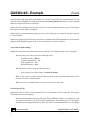
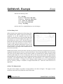
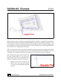
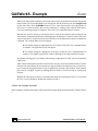
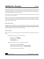
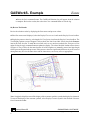
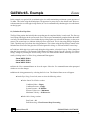
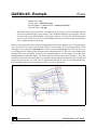
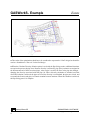
GASWorkS™ Example
Estate
Summary
In this example, a new model will be created for a small housing estate. A DXF file of the estate layout will
be used as a background to the model schematic. The model will be created by tracing over the layout.
Customers will be added along the new mains. The diversified load will be calculated. The pipe sizing
routine will be used to select appropriate pipe sizes for the new system.
Steps
The following assumes that GASWorkS has already been started. If a model is already open, close it now
using the Close menu item from the File menu list. Use the following procedure to work this example...
1) Create Default Settings File
When GASWorkS is first installed it is generally setup for traditional US dimensional units. In this example
we will use units common to the UK gas industry. A default settings file containing UK settings for a low
pressure system is included in the sample files. To review the file:
! Select the Set Defaults menu item from the Utilities menu list. The Default Data Values screen will appear.
! Select the Retrieve Settings command button. The File Selection screen will appear. Find and
select the file named uk.dfs. Select the Continue command button.
! Review the settings by viewing the contents of each data tab. When done reviewing the settings, select the
Close command button to exit the screen and save the values.
2) Create The New Model
! Select the New Project menu item from the File menu list. The Project Specifications screen will appear.
Enter or select the following values.
Model Name = Leave As Default Name or Enter New Name
Header Template = Default
Preference Settings = Default
Default Settings = uk
Facility Settings = Default
Pipe/Main Sizing Table = uk_pipe
Attach A Linked Customer Attribute File = Unselected (Unchecked)
Attach A Linked Pipe Attribute File = Unselected (Unchecked)
Bradley B Bean PE
ENGINEERING & SOFTWARE
Revision - 001, Copyright 2015, All Rights Reserved.
1
GASWorkS™ Example
Estate
! Set the background image file by selecting the Select From Existing DXF Files command button. The File
Selection screen will appear. Find and select the file named estate_plat.dxf. Select the Continue command
button to assign the file to the specification.
! After the above settings have been made, select the Continue command button to proceed. The Graphic
Data Interface (GDI) window will appear.
! If the model is not automatically displayed, select the View/Edit menu item from the Graphics menu list
to view the model.
! Resize the image using the Maximize GDI Window command in the GDI Command List. Then zoom the
image to fill the display using the Zoom To Fit icon from the View Controls toolbar.
3) Set Some Graphic Settings
! Select the Settings menu item from the Graphics menu list. The Graphic Settings screen will appear.
! In the Settings list, enter or select the following values:
Coordinates Units = Metres
Customer Symbol Size = 3%
Node Symbol Size = 1%
Refresh Increment = 10%
! In the Options section, select the following values:
Query During New Feature Entry = Selected (Checked)
Note - If you want to save these settings so that you do not need to reset them in the future, select
the Save As Default command button.
! Select the Close command button to exit the screen and save the values.
4) Set Property Files
! Select the Property Tables menu item from the Preferences submenu of the File menu list. The Property
Tables Selection screen will appear.
! If the standard property table path (\Program Files\GASWorkS 9\Prop\) is not displayed as the
current path, select the Change Path Setting command button. The Path Settings screen will appear,
find and select the appropriate directory/folder. Select the Close command button to save the change.
Bradley B Bean PE
ENGINEERING & SOFTWARE
Revision - 001, Copyright 2015, All Rights Reserved.
2
GASWorkS™ Example
Estate
! Enter the following values:
Pipe = uk_pipe
Regulator = Select Any Valid Table
Compressor = Select Any Valid Table
Valve = Select Any Valid Table
Well = Select Any Valid Table
Fittings = uk_fitting
! Select the Close command button to save the changes.
5) Check Image Scale
! Zoom into the lower right portion of the image where
the “hammer head” appears using the Zoom Window
command. To use the command select the Zoom
Window icon from the View Controls toolbar. Move the
mouse pointer to a location slightly to the upper left of
the area that you want to view, click the left mouse
button. Move the mouse pointer to a location slightly to
the lower right of the area that you want to view (a
window or box should be drawn on the screen as you
move the mouse), click the left mouse button at the
second location. The image will be zoomed to fit the
selected zoom window.
! Measure the distance between the inner east and west portions of the feature using the Measure Distance
command. Select the Measure Distance icon from the Graphic Utility Commands toolbar. For the first point
click (press the left mouse button when the mouse pointer is positioned at the desired location) on the
western (north-south) line. For the second point click on the eastern (north-south) line approximately
perpendicular to the first point, then press the right mouse button to indicate that the measurement selection
is complete. The measured distance will be displayed. The actual distance is 21.5 Metres, the displayed
distance should be within +/- 0.5 Metres. If it is, continue with the example. If it is not, something has not
been set correctly, perhaps a coordinate or length dimensional unit - check the values and revise as
appropriate.
6) Enter The Piping System
The goal of this example is to produce a design similar to one shown in Figure 1. The supply or source
location is in the lower left (southwest) corner of the estate.
Bradley B Bean PE
ENGINEERING & SOFTWARE
Revision - 001, Copyright 2015, All Rights Reserved.
3
GASWorkS™ Example
Estate
Figure 1
Note - In general, a pipe is entered by selecting the appropriate “Add Pipe” command, entering the From
Node Location, entering vertex locations (deflection points on a polyline), then finally entering the To Node
Location. Because we selected the Query During New Feature Entry option in the Graphics Settings, a data
box will appear each time a new node or pipe feature is entered. When this occurs, enter the appropriate data,
then select the Close command button to continue.
Note - You will need to use the Zoom and Pan commands to display a portion of the background to a suitable
scale as you add the new pipe segments. If you are not already familiar with these commands, refer to the
GASWorkS User’s Manual or Help Guide for instructions on using the Zoom and Pan commands.
! We will start at the supply point and work around
the estate entering pipes as we go. Zoom to a
suitable image view using an appropriate Zoom
and/or Pan command (see Figure 2 for location).
! Enter the first pipe by selecting the Add
Polyline Pipe icon from the Graphic
Construction Commands toolbar. Draw the
new pipe.
Figure 2
Bradley B Bean PE
ENGINEERING & SOFTWARE
Revision - 001, Copyright 2015, All Rights Reserved.
4
GASWorkS™ Example
Estate
! Select the From Node location by moving the mouse to the desired location and pressing the left
mouse button. The From Node Data screen will appear. On the Hydraulic tab, enter Supply Point
for the Node Name. Enter 30 MilliBar for the Pressure value. Because this is the supply point, set
the Pressure as known and the Base Load as unknown by clicking in the adjacent check boxes.
Leave the remaining settings as displayed. Select the Close command button to continue.
! Select any desired vertices by moving the mouse to the desired location and pressing the left
mouse button. Continue until all of the remaining points, including the To Node Location, have been
entered. After the To Node Location has been entered, press the right mouse button to terminate the
command. The To Node Data screen will appear.
! The default settings are appropriate for the To Node. Select the Close command button
to continue. The Pipe Data screen will appear.
! The default settings are appropriate for the pipe. Select the Close command button to
continue. The graphic image will be redrawn showing the new pipe and node locations.
! Continue entering pipes by panning and zooming as appropriate to work your way around the
subdivision.
Note - When entering the From Node Location for a new pipe, notice that default location is for the
most previous entered node. If you want the new pipe to continue from the last node, press the Enter
key to accept the displayed location. If you are graphically selecting a node location, ensure that the
pipe ends are “snapped” together by holding down the Shift key when selecting an existing node
location.
! When all of the pipes are entered - zoom the entire image by selecting the Zoom To Fit icon from
the View Controls toolbar. It should look similar to Figure 1.
7) Enter The Customer Locations
In this example a customer data feature will be entered for each potential customer location, similar to Figure
3.
Bradley B Bean PE
ENGINEERING & SOFTWARE
Revision - 001, Copyright 2015, All Rights Reserved.
5
GASWorkS™ Example
Estate
Figure 3
Note - In general, a customer is entered by selecting the appropriate “Add Customer” command, entering the
customer location, then depending on the command, indicating which pipe (main) the customer is supplied
from. We will use an “auto” assign command so the main will automatically be assigned - we will not need
to identify the supply main. Customer default data is handled different than the pipe and node data. Default
customer data is set by extracting the data contents from the last entered customer and applying it to the
customer being entered. Depending on the “add” command selected, a data screen will appear each time a
new customer is entered. When this occurs, enter the appropriate data, then select the Close command button
to continue.
! Select the Add Multiple Customers - Auto Assign Main icon from the Customer Data Commands toolbar.
Select the location of the first customer by moving the mouse pointer to the desired location and pressing
the left mouse button. The Customer Data screen will appear.
! Enter the following values:
Load Application = Diversified, Wet Central Heat - Post 1977
Adjust Load By Design Factor = Unselected (Unchecked)
Status = On
Unit Count = 1
Per Unit Load = -20000 kWh
! Leave the remaining settings as displayed. Select the Close command button to save the changes.
Bradley B Bean PE
ENGINEERING & SOFTWARE
Revision - 001, Copyright 2015, All Rights Reserved.
6
GASWorkS™ Example
Estate
! A prompt will appear to enter the location of the next Customer. Select the desired customer location by
moving the mouse pointer to the desired location, then click the left mouse button. The customer will
automatically be assigned to the closest main. If the main selected by the routine is not the desired main, it
can be changed after all of the customers are entered.
! Continue entering the remaining customer locations. Press the right mouse button after the last customer
as been entered, to end the command.
Note - The Customer Data screen will only appear for the first customer. When using the Add Multiple
Customers -Auto Assign Main command, it is assumed that all of the customers will have the same data
values associated with them. If a customer has a different set of values, it can be individually revised using
the Edit Customer Data command.
8) Spot Check The Data
Check the customer assignments. If an incorrect assignment is found, use the Reassign Supply Main
command to correct it. To use this command select the Reassign Supply Main icon from the Customer Data
Commands toolbar. Select the customer to be changed. Select the new supply main by moving the mouse
pointer near the desired main, then click the left mouse button.
9) Solve The Model
! Select the Solve icon in the lower right hand corner of the GDI window. The Solution Data screen will
appear.
! On the Other Settings tab, enter the following values:
Base Pressure = 1013 Millibar
Base Temperature = 15.6 Celsius
Upper Dampening = 0
Lower Dampening = 0
! On the Solution Data tab, enter or select the following values:
Calculate Diversity = Selected (Checked)
Reset Unknown Node Pressures To Zero = Selected (Checked)
Smart Processing Of One-way Segments = Selected (Checked)
• Review the remaining solution parameters.
Bradley B Bean PE
ENGINEERING & SOFTWARE
Revision - 001, Copyright 2015, All Rights Reserved.
7
GASWorkS™ Example
Estate
! Select the Solve command button. The GASWorkS Solution Log will appear when the solution
is complete. Review the results, then select the Close command button to exit the log.
10) Review The Results
Review the solution results by displaying the flow arrows and pressure values.
! If the flow arrows aren't displayed, select the Display Flow Arrows icon from the Display Controls toolbar.
! Display the pressure values by selecting the Set Text Options icon from the Display Controls toolbar. The
Text Display Options screen will appear. Select (check) the Node Items label. Select (check) the Pressure
item in the Node Item list. To make the text a little easier to see, unselect (uncheck) the Transparent Font
option. Select the Apply command button to update the display. The values should be similar to those shown
in Figure 4. They will not be the same because all of the lengths were manually entered, and pipe length
affects pressure drop and node pressures. If the pressure values are significantly different, any error occurred
during data entry. Review the data values and the instructions, correct any errors as appropriate.
Figure 4
Note - It might be helpful to turn off the display of the customer symbols, to make the display less cluttered.
To turn off the display of the customer symbols, select Display Customer Symbols icon from the Customer
Data Commands toolbar.
Bradley B Bean PE
ENGINEERING & SOFTWARE
Revision - 001, Copyright 2015, All Rights Reserved.
8
GASWorkS™ Example
Estate
In this example, our goal will be to minimize pipe sizes while maintaining a minimum system pressure of
21 mBar. The results using the default pipes sizes appear to be pretty close to the desired result. However,
to demonstrate the use of the pipe sizing routine, let’s use it to automatically calculate pipe sizes which meet
our design goal.
11) Calculate New Pipe Sizes
The Pipe Sizing routine has basically three steps that must be completed before it can be used. The first step
is to indicate which pipes in the system can be sized. This step was automatically completed when the model
was built. The default data was set such that the pipe sizing option was selected for the pipes, as they were
entered. The second step is to indicate which pipe sizes can be used. This is done using the Pipe Properties
Table. The third step is to indicate the sizing parameters. This is done using the Pipe Sizing Controls in the
Solution Data. Since all of the pipes have been designated for sizing, we will start with the second step.
! To indicate which pipe sizes can be used during the sizing routine, select the Property Tables menu item
from the Report menu list. The Property Table Report will appear. On the Pipe tab, clear the “Use When
Sizing” settings by selecting the Set All Settings To No icon. Then indicate that the following sizes can be
used by clicking in the Use When Sizing column until Yes appears:
32mm MDPE SDR11
63mm MDPE SDR11
90mm MDPE SDR11
! Select the Close command button to close the report. Select the Yes command button when prompted
whether to save the changes.
! Indicate the sizing parameters by selecting the Solve icon. The Solution Data screen will appear.
! On the Pipe Sizing Control tab, enter or select the following values:
! In the Limit/Check Values section:
Condition Nodes = Empty
Condition Pressure = Empty
System Pressure = 21 Millibar
Pressure Values Are = Minimums
Maximum Velocity = 20 Metres/sec
!In the Other Settings section:
Pass Limit = 30
Path Processing = Flow-Pressure Drop Processing
Bradley B Bean PE
ENGINEERING & SOFTWARE
Revision - 001, Copyright 2015, All Rights Reserved.
9
GASWorkS™ Example
Estate
Optimize By = Size
Facility Type = All Facility Types
Reset Diameters To Minimum Size = Selected (Checked)
Pipe Size Table = uk_pipe
! After the values have been entered, select the Solve & Calculate Pipe Sizes command button to
execute the solution and pipe sizing routines. The GASWorkS Solution Log will appear. Note the
last entry on the log. It should display, “Pipe Sizing Complete”. If it does, the Pipe Sizing routine
was successful. If it does not, an error occurred during data entry. Review the results, then select the
Close command button to exit the log.
! Review the results of the sizing routine by displaying the node pressures and pipe sizes. To display the pipe
sizes, select the Set Text Options icon from the Display Controls toolbar. The Text Display Options screen
will appear. Select (check) the Pipe Items label. Select (check) the Size/Type item in the Pipe Items list.
Let’s change the color of the pipe text. Select the color swatch below the Pipe Items list. Select another color
(perhaps black) from the pallette. Select the OK command button to save the change. Select the Apply
command button to update the display. The values should be similar to those shown in Figure 5. They may
not be the same because all of the lengths were manually entered, and pipe length affects pressure drop and
pressure drop affects pipe size. If the sizes are significantly different, an error occurred during data entry.
Review the data values and the instructions, correct any errors as appropriate.
Figure 5
Bradley B Bean PE
ENGINEERING & SOFTWARE
Revision - 001, Copyright 2015, All Rights Reserved.
10
GASWorkS™ Example
Estate
Note - The Pipe Sizing routine yields different results depending on a variety factors one of which is the
“processing method”. Generally the method that was specified for this example (Flow-Pressure Drop
Processing) yields the most acceptable results. Depending on the pipe lengths, pipe segmentation, and
customer assignment associated with your model, your results will vary from those shown here.
Notes & Considerations
! In this example, an existing DXF file was used to create a background to trace over. We assumed the
drawing was to scale and our check indicated that it was. What if it wasn't? Ideally we would go back to the
original drawing and rescale it in the CAD system used to create the DXF. This would ensure that next time
we used the file it would be to scale. If it is not possible to get access to the original file or you do not have
a way of re-scaling the DXF file, the scale and shift values in the background image settings could be used
to adjust the image before tracing over it.
! The model loads only represent the loads of the customers immediately attached to the system. We
probably should consider whether additional loads need to be applied to account for future growth.
! The supply pressure was given in this example. In reality if the supply was from a non-regulated (nongoverned) source, for example a main line connection, the supply pressure would need be derived from an
analysis of the upstream system, or from field data collected from pressure recording charts or gauges. In
either case, for a complete analysis, the impact of the new system on the upstream system should be
considered. Adding load to the upstream system will cause the upstream pressures to be reduced, and may
negatively impact both the existing and new system's performance.
! In this example, the Optimization routine was used to select new pipe sizes required to achieve a design
which meet certain design limitations. The results of the optimization were not unreasonable but probably
not necessarily the way most folks would design the system. For example, in this case the Pipe Sizing routine
has oversized the first segment. The segment could be downsized from 90mm to 63mm while maintaining
the system pressures within the design limits - see Figure 6.
Bradley B Bean PE
ENGINEERING & SOFTWARE
Revision - 001, Copyright 2015, All Rights Reserved.
11
GASWorkS™ Example
Estate
Figure 6
! The results of the optimization should never be considered to represent the "final" design, but should be
used as a foundation or "first-cut" for the final design.
! When the Calculate Diversity Solution option is used with the Pipe Sizing routine, additional iterations
are required to process the pipe sizes. Because diversity is affected by pipe flow (customers are assigned at
the downstream end of their associated pipe), when a pipe is resized, the flow in the pipe also changes changing the diversity associated with that pipe. So when a diversity calculation is included, an initial
diversified solution is achieved, the pipes are sized, the diversity is recalculated, the pipes are resized, and
so on until the diversity and pipe sizes remain constant between iterations. When this condition is achieved,
the Pipe Sizing process is complete.
Bradley B Bean PE
ENGINEERING & SOFTWARE
Revision - 001, Copyright 2015, All Rights Reserved.
12