Download Polylib User`s Manual

Polylib User’s Manual
The Polylib Team
September 26, 2002
Contents
1 Introduction
On polyhedra . . . . . . . . . . . . . . . . .
What is Polylib useful for? . . . . . . . . .
To know more about polyhedra and Polylib
About the organization of Polylib . . . . . .
What does the user’s manual contain? . . .
.
.
.
.
.
.
.
.
.
.
.
.
.
.
.
.
.
.
.
.
.
.
.
.
.
.
.
.
.
.
.
.
.
.
.
.
.
.
.
.
.
.
.
.
.
.
.
.
.
.
.
.
.
.
.
.
.
.
.
.
.
.
.
.
.
.
.
.
.
.
3
3
4
4
5
5
2 Getting started
2.1 A very simple example . . . . . . . . . . .
2.2 Using Polylib for solving it . . . . . . . .
2.2.1 Install the library . . . . . . . . . .
2.2.2 Write the C program . . . . . . . .
2.2.3 Write the input to the C program
2.2.4 Compile and run the C program .
.
.
.
.
.
.
.
.
.
.
.
.
.
.
.
.
.
.
.
.
.
.
.
.
.
.
.
.
.
.
.
.
.
.
.
.
.
.
.
.
.
.
.
.
.
.
.
.
.
.
.
.
.
.
.
.
.
.
.
.
.
.
.
.
.
.
.
.
.
.
.
.
.
.
.
.
.
.
6
6
6
7
8
8
9
.
.
.
.
.
3 Matrices and vectors
11
3.1 Basic operations on elementary data structures . . . . . . . . . . 11
3.2 Vector operations . . . . . . . . . . . . . . . . . . . . . . . . . . . 12
3.3 Matrix operations . . . . . . . . . . . . . . . . . . . . . . . . . . 14
4 Polyhedra
4.1 Theoretical background . . . . . . . . . . . .
4.2 Main functions in Polyhedron.c . . . . . . .
4.2.1 Computing on Domains or polyhedra .
4.2.2 Chernikova level functions . . . . . . .
.
.
.
.
.
.
.
.
.
.
.
.
.
.
.
.
.
.
.
.
.
.
.
.
.
.
.
.
.
.
.
.
.
.
.
.
.
.
.
.
.
.
.
.
16
16
19
19
21
5 Lattices
23
5.1 Theoretical background . . . . . . . . . . . . . . . . . . . . . . . 23
5.2 Important functions in Lattice.c . . . . . . . . . . . . . . . . . . 25
6 Z-Polyhedra
27
6.1 Theoretical background . . . . . . . . . . . . . . . . . . . . . . . 27
6.2 Main functions of Zpolyhedron.c . . . . . . . . . . . . . . . . . 28
7 Parametrized polyhedra and Ehrhart polynomials
7.1 Theoretical background . . . . . . . . . . . . . . . .
7.1.1 Parameterized polyhedra representation . . .
7.1.2 Parameterized vertices representation . . . .
7.1.3 Ehrhart polynomials representation . . . . .
1
.
.
.
.
.
.
.
.
.
.
.
.
.
.
.
.
.
.
.
.
.
.
.
.
.
.
.
.
30
30
30
31
31
7.2
7.3
Main functions in polyparam.c . . . . . . . . . . . . . . . . . . . .
Main functions and variables in ehrhart.c . . . . . . . . . . . . .
8 Other tools
31
32
34
9 Data structures
9.1 Basic types . . . . . . . . . . . . .
9.1.1 Integer representation . . .
9.1.2 Error handling . . . . . . .
9.1.3 The saturation matrix . . .
9.2 The homogeneous representation of
9.3 Matrices and Polyhedra . . . . . .
9.4 Lattices and Z-polyhedra . . . . .
9.5 Parametrized Polyhedra . . . . . .
. . . . . . . .
. . . . . . . .
. . . . . . . .
. . . . . . . .
affine spaces
. . . . . . . .
. . . . . . . .
. . . . . . . .
.
.
.
.
.
.
.
.
.
.
.
.
.
.
.
.
.
.
.
.
.
.
.
.
.
.
.
.
.
.
.
.
.
.
.
.
.
.
.
.
.
.
.
.
.
.
.
.
.
.
.
.
.
.
.
.
.
.
.
.
.
.
.
.
.
.
.
.
.
.
.
.
10 Example
37
37
37
37
37
38
39
40
41
42
11 Installation
11.1 Hardware and software requirements
11.2 Installation procedure . . . . . . . .
11.3 Options of the configure script . . .
11.4 Known problems . . . . . . . . . . .
2
.
.
.
.
.
.
.
.
.
.
.
.
.
.
.
.
.
.
.
.
.
.
.
.
.
.
.
.
.
.
.
.
.
.
.
.
.
.
.
.
.
.
.
.
.
.
.
.
.
.
.
.
.
.
.
.
.
.
.
.
.
.
.
.
46
46
46
47
49
Chapter 1
Introduction
Polylib is a free C library for doing computations on polyhedra. The library
is operating on objects like vectors, matrices, lattices, polyhedra, Z-polyhedra,
unions of polyhedra and other intermediary structures. It provides functions for
all important operations on these structures.
Polylib can be downloaded from http://www.irisa.fr/polylib/
This document is Polylib user’s manual. It contains the information needed
to understand what Polylib does, how it can be installed, and a few words about
how it is implemented.
In this introduction, we first describe polyhedra, then we present the applications of Polylib, we develop a little bit the relationship between polyhedra
and parallelization techniques, we provide a few references, we present the organization of Polylib, and finally, we present the remaining of the document.
We are continuously maintaining the library. If you have any comment or
question about this document or the library itself, please feel free to contact us
(http://www.irisa.fr/polylib)
On polyhedra
The polyhedral theory derives from the theory of linear and integer programming.
A convex polyhedron has two dual representations: it can be seen as the
intersection of a finite number of half spaces, or as a combinations of vertices,
rays and lines. The first representation is also called implicit representation
while the second one is called the parametric representation (or generator representation as every point in a polyhedral domain can be generated by a linear
combination of its generators). In order to avoid any misunderstanding between
the parametric representation and the parameterized polyhedra in the following
we will call it Minkovski representation.
Motzkin [MRTT] introduced the double representation method, a general
non-pivoting technique for solving the dual-computation for a cone. Chernikova
algorithm [Che65] showed how to pass from one representation to the other in
the restricting case of non-negative variables. Chernikova’s algorithm received
successive improvements [FQ88, Le 92] which resulted eventually in an efficient
computation kernel that forms the basis for polyhedra computations.
Polylib uses a double description form for representing polyhedra (actually,
3
finite unions of polyhedra). The computation of one representation from the
other is realized with Chernikova’s algorithm. Based on this algorithms, Polylib
implements a variety of polyhedra operations, such as intersection, complement,
etc.
Polylib also manipulates affine functions (and image and pre-image of polyhedra) and permits to compute difference between two polyhedra. It also extends the concept of polyhedra to Z-polyhedra, that is to say, the intersection of
polyhedra and lattices. Finally, Polylib computes parameterized polyhedra and
coputes Ehrhart polynomials to find the number of integer points in a union of
rational convex polytopes.
What is Polylib useful for?
A polyhedral library can be used in various fields: In computational geometry,
combinatorial optimization, program optimization and parallelization, program
verification, . . . Polylib was developed while working on parallelization techniques, and its main users belong to this community. This is the reason why we
give here more information on this domain.
The iteration domain of a loop nest can be represented by a convex polyhedron, each integral point representing a vector of iteration indices. Therefore,
operations on polyhedra are useful for doing loop transformations and other
program restructuring transformations which are needed in parallelizing compilers.
Along the same lines, polyhedra are a means of describing domain definitions
of variables in systems of affine recurrence equations, a formalism introduced
at the end of the sixties (of the last century!) to model parallel computations.
Therefore the development of methods to do synthesis, analysis and verification
of systems of recurrence equations requires also polyhedra computations. By
means of such methods one can transform an algorithm from a mathematical
description into an equivalent form that can be implemented either with special
purpose hardware (with systolic arrays for instance) or as a program which can
be run on a multiprocessor system.
To know more about polyhedra and Polylib
To know more about polyhedra and Polylib, the following references can be
consulted:
• A. Schrijver’s book [SCH86]: Theory of Linear and Integer Programming.
• D. K. Wilde’s report [Wil93] : A library for doing polyhedral operations
• S. P. K. Nookala and T. Risset [NRi00] A library for Z-Polyhedral operations
• Polylib reference manual
• V. Loechner [Loe99] Polylib:A library for Manipulating Parametrized Polyhedra
4
• K. Fukuda Polyhedral computation FAQ,
http://www.ifor.math.ethz.ch/ fukuda/fukuda.html
See also the links part of the Polylib web site.
About the organization of Polylib
Polylib is written in Ansi C and is running on Unix, Linux, and Windows
(provided Cygwin is installed). Polylib is evolving, and developed by Brigham
Young University, ICPS in Strasbourg , LIP in Lyon and Irisa in Rennes. The
sources of the library can be accessed via the central CVS repository in Rennes
at url: http://www.irisa.fr/cgi-bin/cvsweb.cgi/
Polylib is free, but is subject to the GNU General Public Licence agreement.
Currently, Polylib does not provide a user-friendly interface for computing polyhedra: if you want to try it, you have to write a C program which calls the
appropriate functions (see chapter 2 and annexe 10 for detailed explanations).
What does the user’s manual contain?
This document contains the following chapters.
• Chapter 2 present a rapid introduction of how to use the library.
• Chapter 3 describes matrix and vector routines of Polylib.
• Chapter 4 presents notions on polyhedra, and lists the main C functions
on polyhedra of Polylib.
• Chapter 5 describes lattice functions of Polylib.
• Chapter 6 describes functions of Polylib dealing with Z-polyhedra.
• Chapter 7 describes functions of Polylib dealing with parameterized polyhedra and Ehrhart polynomials.
• Chapter 8 describes a few additional tools of Polylib.
• Chapter 9 presents briefly the data structures of Polylib.
• Chapter 10 shows a short program that may serve as exemple of using
Polylib.
• Chapter 11 provides the necessary information to install Polylib.
5
Chapter 2
Getting started
This section is dedicated to the explanation of a very simple use of the Polylib
by a new user. It can be skipped by people who have already used the library.
2.1
A very simple example
Consider the C code of figure 2.1, and imagine you want to know exactly which
part of array A is accessed in both loop nests.
for (i=1;i<=N;i++)
for (j=1;j<= i; j++)
A[i][j]=0;
for (i=1;i<=N;i++)
for (j=1;j<= N; j++)
if (i+j>=N) A[i][j]=1;
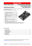
Figure 2.1: two simple nested loops, N is a size parameter, not known at compile
time.
As array A is addressed with identity function, the element of A accessed
in memory directly correspond to the values taken by vector (i, j) during the
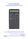
execution. The iteration space of the first loop is D1 = {i, j | 1 ≤ i ≤ N ; 1 ≤
j ≤ i} (see figure 2.2-(a)), the value of (i, j) accessed in the second loop nest
correspond to the polyhedron: D2 = {i, j | 1 ≤ i ≤ N ; 1 ≤ j ≤ N ; i + j ≥
N } see figure 2.2-(b)). On figure 2.2, we have represented these polyhedra as
well as the integer points contained in these polyhedra. Remind that, unless
otherwise specified, Polylib manipulates sets of integer points contained in a
polyhedron. The solution of the problem is simply obtained by intersecting
these two polyhedra: D3 = D1 ∩ D2 = {i, j | 1 ≤ j ≤ i ≤ N ; i + j ≥ N } (see
figure 2.2-(c)).
2.2
Using Polylib for solving it
This problem (computing the intersection of two given polyhedra) can be solved
by writing a C program that calls the functions defined in Polylib. For this, you
6
Figure 2.2: Polyhedra modeling the iteration spaces of the two loop nests of
figure 2.1 for N=5: (a) and (b), and the intersection of them: (c).
have to perform the following steps: install the library, write the C program,
write the input to the C program, compile and run the C program.
2.2.1
Install the library
The precise explanations of the installation procedure are present in chapter 11,
we briefly explain the main steps here. The following commands correspond to
an execution on a Sparc station under Solaris operating system. The commands
are quite identical on Windows (using cygwin) and linux platform.
1. Download the library (e.g. file polylib5.0.tgz at url :
http://www.irisa.fr/polylib/).
2. Decompress the archive:
gunzip polylib5.0.tgz
tar xvf polylib5.0.tar
This will create the Polylib directory where all Polylib files are.
3. Configure the makefile (for instance, if you want a 32 bit integer version):
cd Polylib
./configure --enable-int-lib
4. Compile the library (and run the tests):
make
make test
This installation procedure will place a library file called libpolylib32.a in directory Polylib/Obj.32.sparc-sun-solaris2.6/. This location can be modified by giving options to the configure script (see chapter 11).
7
2.2.2
Write the C program
The C program is represented in figure 2.3. The domains D1 and D2 will be entered to the program as constraints (implicit representation) because this is the
most intuitive way of representing them given the original problem. Hence, we
use the Matrix Read function to read them. Then, these constraints have to be
translated to polyhedra (i.e. the parametric representation has to be computed
by the Chernikova algorithm). Hence the use of the Constraints2Polyhedron
function (in the program of figure 2.3, we allow the domains to have 200 constraints or less). Finally we can intersect the polyhedra (DomainIntersection
function) and print out the result.
#include <stdio.h>
#include <polylib/polylib.h>
int main() {
Matrix *a1, *a2;
Polyhedron *D1, *D2, *D3;
a1 = Matrix_Read();
a2 = Matrix_Read();
D1 = Constraints2Polyhedron(a1, 200);
D2 = Constraints2Polyhedron(a2, 200);
D3 = DomainIntersection(D1,D2,200);
printf("\n D3 =");
Polyhedron_Print(stdout,P_VALUE_FMT,D3);
}
Figure 2.3: C program (file prog1.c) for solving the problem of section 2.1 with
Polylib
2.2.3
Write the input to the C program
The input format needed by the Matrix read function
is quite
¢ unconvenient.
¡
A constraint (say ~a · ~x ≥ b) is represented in a row ~a −b of a matrix. In
addition, as Polylib handles equality and inequalities, the first column of this
matrix will be a 1 (for inequality) or a 0 (for equality).
Hence, the¢ constraint
¡
i + 2j >= 3 will correspond to a the following row: 1 1 2 −3 (assuming
that i and j are the only indices and that we have chosen to order them in the
order (i, j)).
In our case, we have to enter the constraint corresponding to domain D1 =
{i, j | 1 ≤ i ≤ N ; 1 ≤ j ≤ i}. In Polylib, you have to consider N as an index
8
hence, the constraints of domain D1 could be represented in matrix form as:



−1 0 1 0
i
 1


0 0 −1 

 j  ≥ 0
 0


1 0 −1
N 
1 −1 0 0
1
Similarly a possible matrix form for the constraints of D2 = {i, j | 1 ≤ i ≤
N ; 1 ≤ j ≤ N ; i + j ≥ N } could be:




−1 0
1
0
i

 1
0
0 −1  


 0 −1 1
 j 
0 
 N  ≥ 0

 0
1
0 −1 
1
1
1 −1 0
From these matrices, we deduce the input file to be written which is represented
in figure 2.4.
4
1
1
1
1
5
1
1
1
1
1
5
-1 0 1
1 0 0
0 1 0
1 -1 0
5
-1 0 1
1 0 0
0 -1 1
0 1 0
1 1 -1
0
-1
-1
0
0
-1
0
-1
0
Figure 2.4: The input file (file prog1.in) to program of figure 2.3
Writing the input file of figure 2.4 is painful, you can use the programs
readPol and writePol that translate back and forth form the external format
of polyhedra (like : {i,j | 1<=i<= N; 1<=j<=i }) and the internal input
format used in figure 2.4 (see the ”interesting links” on http://www.irisa.fr/
polylib).
2.2.4
Compile and run the C program
Here, we decompose the compilation into compiling and linking to make things
clear. We assume that prog1.c is situated just above the Polylib directory
(the -D flag indicates to the compiler, which type of integer you are using). The
compilation command is:
gcc -c -g -O2 -I Polylib/include -DLINEAR_VALUE_IS_INT prog1.c -o prog1.o
Then link it with the library to provide an executable.
gcc prog1.o Polylib/Obj.32.sparc-sun-solaris2.6/libpolylib32.a -o prog1
9
In general it might be better to use a makefile for compiling the C program, because many flags are set up in the file vars.mk. A sample Makefile is provided
in the example of the Polylib) hierarchy.
Finally, run the program on the input file of figure 2.4.
prog1 < prog1.in2
The output of the execution shown on figure 2.5. In this output form, the first
column of the matrix is translated into:£ Inequality or¤ equality. Hence, for
1 −1 0 0 should be read as i ≥
instance, the first row: Inequality:
j. One can check that it corresponds to D3 = {i, j | 1 ≤ j ≤ i ≤ N ; i + j ≥ N }
Of course, Polylib should be used to solved more complex problem and it is
specifically dedicated to serve as a kernel library in a bigger program and not
as a stand-alone program.
D3 =POLYHEDRON Dimension:3
Constraints:5 Equations:0
Constraints 5 5
Inequality: [
1
-1
0
0 ]
Inequality: [
1
1
-1
0 ]
Inequality: [ -1
0
1
0 ]
Inequality: [
0
1
0
-1 ]
Inequality: [
0
0
0
1 ]
Rays 5 5
Ray:
[
1
0
1 ]
Ray:
[
1
1
1 ]
Ray:
[
1
1
2 ]
Vertex: [
1
1
2 ]/1
Vertex: [
1
1
1 ]/1
Rays:5
Lines:0
Figure 2.5: Result of the execution of the program of figure 2.3 on the input file
of figure 2.4
10
Chapter 3
Matrices and vectors
As any polyhedral operation exploits structures like matrices, vectors or values,
Polylib provides elementary functions on these data structures. This chapter is
devoted to these functions. Section 3.1 presents the basic operations. Section 3.2
describes operations on vectors. Finally, section 3.3 presents operations on
matrices.
3.1
Basic operations on elementary data structures
Before going into the details of the available functions, we have to say a word
about the typing mechanism of Polylib (A more complete description of the
data structures of the library is provided in chapter 9). The integer handling
is based on the ArithLib library which was originally part of the Pips compiler (http://www.cri.ensmp.fr/~pips/home.html) developed at the ensmp
in Fontainebleau. In order to handle different integer size (32 bits, 64 bits or
infinite precision with the gmp library), integers are stored in a data structured
called value. At compile time, a value is translated either into 32-bit integer
or 64-bit integer or gmp integer (depending on the options provided during the
compilation). These value are mainly used for the coefficient of the constraints
and ray/vertices of the polyhedra.
Polylib contains a large amount of relational, algebraic or structural operations on integers. Here are some examples of the operations implemented in
Polylib:
• Search for the greatest integer value with the power two less then a given
integer.
int polylib sqrt(int i)
• Least Common Multiple of two values.
void Lcm(value i, value j,value* result)
• Greatest Common Divisor of two values.
void Gcd(value i, value j, value* result)
11
• Factorial for a integer.
void Factorial(int n, value* result)
• Number of ways to choose ’b’ items from ’a’ items.
void CNP(int a, int b, value* result)
In addition, there are some operations that will work only on fixed types.
Exemples are given by MSB, TOP and NEXT functions defined over the integer
type but not on the value type:
• MSB: put a one in the most significant bit of an int.
• TOP: largest representable positive number.
• NEXT(j,b): right shift the one bit in b and increments j if the last bit in
b is one.
3.2
Vector operations
Polylib contains tools for manipulating vector data structures. These functions
are in the file vector.c.
These functions allows the following operations:
• allocating, reading printing or deleting vectors,
• setting a value in each position of a vector,
• sorting values of a vector. This is done in Polylib in the Vector Sort
function using the heap sort algorithm. Other sort operations exists, such
as in function AffinePartSort which perform sorting operation on a list
of lattices.
• unary operations on vectors. Finding the minimum, maximum or greatest
common divisor for a vector. Based on the GCD of a vector other unary
operations are available like Vector Normalize.
• logical operations on vectors components, algebraic computations between
vectors.
Main functions in vector.c
int First Non Zero (Value *p, unsigned length) return the smallest component index in ’p’ whose value is non-zero.
Vector * Vector Alloc (unsigned length): allocate memory space for a
vector.
void Vector Free (Vector *vector): free the memory space occupied by
Vector.
void Vector Print (FILE *Dst, char *Format, Vector *vector): print
the contents of a Vector.
12
Vector * Vector Read () read the components of a vector from the standard
input.
void Vector Set (Value *p, int n ,unsigned length): assign ’n’ to each
component of Vector ’p’.
void Vector Exchange : exchange the components of the vectors ’p1’ and
’p2’.
void Vector Copy (Value *p1, Value *p2, unsigned length): copy vector ’p1’ to vector ’p2’.
Vector Add (Value *p1, Value *p2, unsigned length): add two vectors
’p1’ and ’p2’ and store the result in ’p3’.
void Vector Sub (Value *p1, Value *p2, Value *p3, unsigned length):
subtract two vectors ’p1’ and ’p2’ and store the result in ’p3’.
void Vector Or (Value *p1, Value *p2, Value *p3, unsigned length):
compute bit-wise OR of vectors ’p1’ and ’p2’ and store it in ’p3’.
void Vector Scale (Value *p1, Value *p2, Value lambda, unsigned
length): scale (i.e. multiply) vector ’p1’ by factor ’lambda’ and store
it in ’p2’.
void Vector AntiScale (Value *p1, Value *p2, Value lambda, unsigned
length): antiscale (i.e. divide) vector ’p1’ by ’lambda’ and store it in ’p2’.
void Inner Product (Value *p1, Value *p2, unsigned length, Value
*result): return the inner product of two vectors ’p1’ and ’p2’.
void Vector Max (Value *p, unsigned length,Value *result): return the
maximum of the components of ’p’.
void Vector Min (Value *p, unsigned length, Value *result): return
the minimum of the components of Vector ’p’.
void Vector Combine (Value *p1, Value *p2, Value *p3, Value lambda,
Value mu, unsigned length): return the linear combination of two vectors.
int Vector Equal (Value *Vec1, Value *Vec2, unsigned n): return 1 if
’Vec1’ equals ’Vec2’, otherwise return 0.
void Vector Min Not Zero (Value *p, unsigned length, int *index,
Value *result): return the component of ’p’ with minimum non-zero
absolute value.
void Vector Gcd (Value *p, unsigned length, Value *result): return
the GCD of components of Vector ’p’.
void Vector Map (Value *p1, Value *p2, Value *p3, unsigned length,
Value *(*f )()): given vectors ’p1’ and ’p2’, and a pointer to a function
returning ’Value’ type, compute p3[i] = f(p1[i],p2[i]).
13
void Vector Normalize (Value *p, unsigned length): reduce a vector by
dividing it by its GCD.
void Vector Normalize Positive (Value *p, int length,int pos): reduce
a vector to a positive vector by dividing it by its GCD.
void Vector Reduce (Value *p,unsigned length,void(*f )(Value,Value
*), Value *result) : reduce ’p’ by operating binary function on its
components successively.
void Vector Sort (Value *vector, unsigned n): sort the components of a
vector ’vector’ using heap sort.
3.3
Matrix operations
Matrix operations in Polylib can be found in three source files:
• matrix.c
• Matop.c
• NormalForms.c
Polylib provides function to:
• allocate, free, read and print matrices,
• compute specific form like the identity matrix, Hermite Normal form (see
page 24), Smith normal forms (see page 35)
• add, remove columns and rows in order to perform basic modifications of
matrices,
• transpose and invert matrices.
Main functions in Matop.c, matrix.c and NormalForms.c
Matrix * Matrix Alloc (unsigned NbRows, unsigned NbColumns): allocate space for matrix of dimensions ’NbRows x NbColumns’.
void Matrix Free (Matrix *Mat): free the memory space occupied by Matrix ’Mat’.
void Matrix Print (FILE *Dst, char *Format, Matrix *Mat): print
the contents of the Matrix ’Mat’.
Matrix * Matrix Read (void) : read the contents of the matrix ’Mat’ from
standard input.
int MatInverse (Matrix *Mat, Matrix *MatInv ): given a integer matrix
’Mat’, compute its inverse rational matrix ’MatInv’.
void rat prodmat (Matrix *S, Matrix *X, Matrix *P): compute the
matrix product between an integer matrix and a rational one.
14
void Matrix Vector Product (Matrix *Mat, Value *p1, Value *p2):
compute the matrix-vector product.
void Vector Matrix Product (Value *p1, Matrix *Mat, Value *p2):
compute the vector-matrix product.
void Matrix Product (Matrix *Mat1, Matrix *Mat2, Matrix *Mat3):
compute the matrix-matrix product.
int Matrix Inverse (Matrix *Mat, Matrix *MatInv ): given a rational
matrix ’Mat’, compute its inverse rational matrix ’MatInv’.
static void transpose (Value *a, int n, int q): transpose a part of a matrix.
static void smith (Value *a, Value *b, Value *c, Value *b inverse,
Value *c inverse, int n, int p, int q): find the Smith Normal Form
of a matrix.
void ExchangeRows (Matrix *M, int Row1, int Row2) : exchange the
rows ’Row1’ and ’Row2’ of the matrix ’M’.
void ExchangeColumns (Matrix *M, int Column1, int Column2): exchange the columns ’Column1’ and ’Column2’ of the matrix ’M’.
Matrix * Transpose (Matrix *A): compute the transpose of a matrix.
int findHermiteBasis (Matrix *M, Matrix **Result): compute the Hermite basis for a matrix (see [NRi00]).
Matrix * Identity (unsigned size): return an identity matrix of size ’size’.
Bool isinHnf (Matrix *A) : check if the matrix ’A’ is in Hermite normal
form.
Matrix * AddANullRow (Matrix *M): add a row of zeros at the end of a
matrix.
Matrix * RemoveColumn (Matrix *M, int Columnnumber): remove a
column from the matrix.
15
Chapter 4
Polyhedra
This chapter has two parts. Section 4.1 presents some theoretical results concerning the theory of polyhedra. Then section 4.2 gives the list of Polylib functions related to the basic part of the library, that is to say, classical polyhedra
representation. These functions can be found in the Polyhedron.c source file
that was one of the first Polylib packages.
4.1
Theoretical background
A nonempty set C of points in a Euclidean space is called a (convex) cone if
λx + µy ∈ C whenever x, y ∈ C and λ, µ ≥ 0. A cone C is polyhedral if
C = {x|Ax ≤ 0}
for some matrix A, i.e. if C is the intersection of finitely many linear half-spaces.
Results from the linear programming theory [SCH86] shows that the concepts
of polyhedral and finitely generated are equivalent.
Theorem 1. (Farkas-Minkowski-Weyl) A convex cone is polyhedral if and only
if it is finitely generated.
A short definition of a polyhedra may be a finitely generated convex cone but
in fact we are talking about the geometric representation of a list of constraints
provided as a linear system of equations and inequalities.
Definition 1. (Polyhedron) A convex polyhedron if it is the set of solutions
to a finite system of linear inequalities. It is called a convex polytope if it is a
convex polyhedron and it is bounded. When a convex polyhedron (or polytope)
has dimension k, it is called a k-polyhedron (k-polytope).
Hence, a set P of vectors in Rn is called a (convex) polyhedron if:
P = {x|Ax ≤ b}
for some matrix A and a vector b, i.e P is the intersection of finitely many affine
half-spaces. In Polylib manipulated objects are -integer polyhedra- which are
integer points on polyhedra.
P 0 = {x ∈ Z n |Ax ≤ b} = P ∩ Z n
16
For simplicity reason, from now on, we refer to polyhedra for integer polyhedra.
The concept of polyhedron and polytope are related by the means of the
decomposition theorem for polyhedra.
Theorem 2. (Decomposition theorem for polyhedra) A set P of vectors in a
Euclidean space is a polyhedron, if and only if P = Q + C for some polytope Q
and some polyhedral cone C.
For a set of vectors a1 , · · · , an , if a vector b does not belong to the cone
generated by these vectors, then there exists a hyperplane separating b from
from a1 , · · · , an . This result has also been formulated in the Farkas’ lemma. A
variant of this result is the following:
Lemma 1. Let A be a matrix and let b be a vector. Then the system Ax ≤ b
of linear inequalities has a solution x, if and only of yb ≥ 0 for each row vector
y ≥ 0 with yA = 0.
In Polylib the decomposition theorem is extensively used (in its extended
form for polyhedra). A polyhedron P can be represented by a set of inequalities (usually, implicit equalities are represented in a separate matrix):
P = {x|Ax = b, Cx ≥ d}, this representation is called implicit. From the
Minkowski characterization, we know that P has a dual representation, called
the parametric representation.
X
P = {x|x = Lλ + Rµ + V ν, where ν ≥ 0,
ν = 1, µ ≥ 0}
Hence, each point of P can be expressed as a sum of:
• a linear combination of so called lines (columns of matrix L),
• a convex combination of vertices (columns of matrix V ), and
• a positive combination of extremal rays (columns of matrix R).
Although the polyhedra theory cannot be detailed here, we review a set of
important concepts that are used when manipulating polyhedra. For a more
precise description, please refer to [SCH86, Wil93].
• The characteristic cone of a polyhedron P = {x|Ax ≤ b} is the polyhedral
cone
char.cone(P ) = {y|x + y ∈ P, ∀x ∈ P } = {y|Ay ≤ 0}
.
Sometimes the characteristic cone is called the recession cone of P . If P =
Q + C, with Q a polytope an C a polyhedral cone, then C = char.cone(P )
.
• The lineality space of P = {x|Ax ≤ b} is the linear space
lin.space(P ) = char.cone(P ) ∩ −char.cone(P ) = {y|Ay = 0}
If the lineality space has dimension zero, P is said to be pointed.
17
.
• A supporting hyperplane of P = {x|Ax ≤ b} is the affine hyperplane
described by {x|cx = δ} where c is a nonzero vector and δ = max{cx|Ax ≤
b}.
• A subset F of a polyhedron P = {x|Ax ≤ b} is called a face if F = P or
if F is the intersection of P with a supporting hyperplane of P . In other
words F is a face if and only if there is a vector c for which F is the set of
vectors attaining max{cx|x ∈ P } provided that this maximum is finite.
A alternative description of a face is the nonempty subset F :
F = {x ∈ P |A0 x = b0 }
for some subsystem A0 x ≤ b0 of Ax ≤ b.
• The faces of a polyhedron P have the following important properties:
– P has finitely many faces;
– each face is a nonempty polyhedron;
– if F is a face of P and F 0 ⊆ F , then: F 0 is a face of P if and only if
F 0 is a face of F .
• A facet of P is a maximal face distinct from P . In other words if there is
no redundant inequality in the polyhedron definition system: Ax ≤ b then
there exists a one-to-one correspondence between the facets of P and the
inequalities given by
F = {x ∈ P |ai x = bi }
for any facet F of P and any inequality ai x ≤ bi from Ax ≤ b .
The faces of dimension 0, 1, k − 2 and k − 1 are called the vertices, edges,
ridges and facets, respectively. The vertices coincide with the extremal
points of the polyhedron, that are also defined as points which cannot be
represented as convex combinations of two other points in the polyhedron.
When an edge is not bounded, there are two cases: either it is a line or a
half-line starting from a vertex. A half-line edge is called an extremal ray.
• The convex hull of a set Q is the convex combination of all points in Q.
It is the smallest convex set which contains all of Q.
Polylib implements procedures to compute, from one representation of a
polyhedron P (implicit of parametric), its dual representation of P , given the
implicit on. The algorithms was proposed by Chernikova [Che65] which rediscovered the double description method introduced by Motzkin. Important
improvements were made in the conversion process between these representations by Fernandez [FQ88] and Le Verge [Le 92].
Based on this kernel algorithm, Polylib propose many computational function on polyhedra. More precisely, Polylib manipulates domains which are finite
unions of polyhedra 1 .
1 The user must be aware of the fact that Polylib is mostly used to represent the set of
integer points contained in domains, hence the set {x|x > 0} (which is not a polyhedron) will,
in fact, represent the set {x|x >= 1}. With this convention, Polylib is able to compute the
difference between polyhedra.
18
Polylib manipulates mixed inhomogeneous system of equations. The terms
inhomogeneous stands for the fact that it manipulates objects of an affine space
(not a linear space). To transform the inhomogeneous affine space of dimension
n into an homogeneous linear space of dimension n + 1, we use the following
mapping:
µ
¶
ξx
M : x −→
,
ξ≥0 .
ξ
With this mapping, a system P = {x | Ax = b, Cx ≥ d} in the original
inhomogeneous space is transformed into C = {x̃ | Ãx̃ = 0, C̃ x̃ ≥ 0} where
µ
¶
µ
¶
ξx
C −d
à = (A − b), x̃ =
and C̃ =
.
ξ
0
1
In the internal representation of Polylib, object manipulated are cones (the
Chernikova algorithm works on cones), but this is transparent for the user which
naturally manipulates polyhedra (or union of polyhedra). As many Polylib
functions refer to domain, we precisely define what a domain is:
Definition 2. (Domain) A polyhedral domain of dimension n is a union of
polyhedra of dimension n.
4.2
Main functions in Polyhedron.c
Here is a brief description of the main functions of Polylib operating on polyhedra. Please refer the the reference manual for a more complete description.
Some of these functions operate on polyhedra (i.e. convex polyhedra) other operate on domains (i.e. unions of polyhedra). Remind that, when using certain
functions (like DomainDifference for instance), the program assume that only
integer points inside the polyhedra are considered.
4.2.1
Computing on Domains or polyhedra
Polyhedron* Polyhedron Alloc (unsigned Dimension, unsigned NbConstraints, unsigned NbRays): allocate memory space for polyhedron.
void Polyhedron Free (Polyhedron *Pol) : free the memory space occupied by the single polyhedron.
void Domain Free (Polyhedron *Pol) : free the memory space occupied
by the domain.
void Polyhedron Print (FILE *Dst,char *Format,Polyhedron *Pol) :
print the contents of a domain.
Polyhedron * Empty Polyhedron (unsigned Dimension) : create and return an empty polyhedron of dimension ’Dimension’.
Polyhedron * Universe Polyhedron (unsigned Dimension) : create and
return a universe polyhedron of dimension ’Dimension’.
Polyhedron * Constraints2Polyhedron (Matrix *Constraints,unsigned
NbMaxRays): given a matrix of constraints ’Constraints’, construct and
return a polyhedron using Chernikova’s algorithm.
19
Matrix * Polyhedron2Constraints (Polyhedron *Pol) : given a polyhedron, extract its matrix of constraints.
Polyhedron * Rays2Polyhedron (Matrix *Ray,unsigned NbMaxConstrs)
: given a matrix of rays (i.e. vertices, rays ans lines) ’Ray’, create and
return a polyhedron using Chernikova’s algorithm.
Matrix * Polyhedron2Rays (Polyhedron *Pol) : given a polyhedron ’Pol’,
extract its matrix of rays (i.e. vertices, rays ans lines).
Polyhedron * AddConstraints (Value *Con, unsigned NbConstraints,
Polyhedron *Pol, unsigned NbMaxRays): add new constraints to a
polyhedron.
Polyhedron * DomainAddConstraints (Polyhedron *Pol, Matrix *Mat,
unsigned NbMaxRays): add constraints to each polyhedron in a polyhedral domain.
Polyhedron * AddRays (Value *AddedRays, unsigned NbAddedRays,
Polyhedron *Pol, unsigned NbMaxConstrs): add rays to a polyhedron.
Polyhedron * DomainAddRays (Polyhedron *Pol, Matrix *Ray, unsigned NbMaxConstrs): add rays to each polyhedron in a polyhedral
domain.
int PolyhedronIncludes (Polyhedron *Pol1, Polyhedron *Pol2): return 1 if ’Pol1’ contains ’Pol2’, 0 otherwise.
Polyhedron * AddPolyToDomain (Polyhedron *Pol, Polyhedron *PolDomain): add Polyhedron ’Pol’ to polyhedral domain ’PolDomain’.
Polyhedron * DomainIntersection (Polyhedron *Pol1, Polyhedron *Pol2,
unsigned NbMaxRays): return the intersection of two polyhedral domains ’Pol1’ an’Pol2’.
Polyhedron * Polyhedron Copy (Polyhedron *Pol): create a copy of a
polyhedron.
Polyhedron * Domain Copy (Polyhedron *Pol): create a copy of a polyhedral domain.
Polyhedron * DomainSimplify (Polyhedron *Pol1, Polyhedron *Pol2,
unsigned NbMaxRays): simplify ’Pol1’ in the context of ’Pol2’: find
the largest domain that, when intersected with polyhedral domain ’Pol2’,
equals ’Pol1’∩’Pol2’.
Polyhedron * DomainUnion (Polyhedron *Pol1, Polyhedron *Pol2, unsigned NbMaxRays): return the union of two polyhedral domains ’Pol1’
and ’Pol2’.
Polyhedron * DomainConvex (Polyhedron *Pol, unsigned NbMaxConstrs): concatenate the lists of rays and lines of the polyhedra of a domain
into one combined list. The result is the convex hull (a polyhedron) of a
domain.
20
Polyhedron * DomainDifference (Polyhedron *Pol1, Polyhedron *Pol2,
unsigned NbMaxRays) : create a new polyhedral domain which is the
difference of two domains.
Polyhedron * Polyhedron Image (Polyhedron *Pol, Matrix *Func, unsigned NbMaxConstrs): compute the image of a polyhedron.
Polyhedron * Polyhedron Preimage (Polyhedron *Pol, Matrix *Func,
unsigned NbMaxRays): compute the preimage of a polyhedron. Note:
Func is not a necessarily invertable. This function computes the set of all
points x such that Func x ∈ Pol.
4.2.2
Chernikova level functions
The following functions represent the core of operations in Polylib. They are
used in the conversion process and work with localy defined types like the saturation matrix. Their declaration is static so they are accessible to all the
functions declared in the file Polyhedron.c but not in any other functions.
In the following descriptions of functions we are using the term ”to saturate”.
As a short definition we can say that a ray or a line saturate a constraint if this
constraint is satisfied with equality. Extensive explanations regarding saturation
matrix can be found in the chapter 9.
struct SatMatrix : the saturation matrix is defined to be an integer (int type)
matrix but it is used at bit level by the Chernikova function: the ith bit
of the j th column is 1 if ray number i saturates constraint j.
static SatMatrix * BuildSat (Matrix *Mat, Matrix *Ray, unsigned
NbConstraints, unsigned NbMaxRays): build a saturation matrix
from constraint matrix ’Mat’ and a ray matrix ’Ray’.
void errormsg1 (char *f , char *msgname, char *msg): errormsg1 is
an external function which may be supplied by the calling program.
static SatMatrix * SMAlloc (int rows, int cols): allocate memory space
for a saturation matrix.
static void SMFree (SatMatrix **matrix): free the memory space occupied by a saturation matrix.
static void SatVector OR (int *p1, int *p2, int *p3, unsigned length):
compute the bitwise OR of two parts of saturation matrices.
static void Combine (Value *p1, Value *p2, Value *p3, int pos, unsigned length): compute the linear combination of two vectors ’p1’ and
’p2’, such that p3[pos]=0.
static SatMatrix * TransformSat (Matrix *Mat, Matrix *Ray, SatMatrix *Sat): return the transpose of the saturation matrix ’Sat’.
static void RaySort (Matrix *Ray, SatMatrix *Sat, int NbBid, int
NbRay, int *equal bound, int *sup bound, unsigned RowSize1,
unsigned RowSize2, unsigned bx, unsigned jx): sort the rays (Ray,
Sat) into three tiers as used in the Chernikova function.
21
static int Chernikova (Matrix *Mat, Matrix *Ray, SatMatrix *Sat,
unsigned NbBid, unsigned NbMaxRays, unsigned FirstConstraint,
unsigned dual): This function is the kernel of Polylib, it computes the
dual of matrix ’Mat’ and place it in matrix ’Ray’.
int Gauss (Matrix *Mat, int NbEq, int Dimension): compute a minimal
system of equations using Gausian elimination method.
static Polyhedron * Remove Redundants (Matrix *Mat, Matrix *Ray,
SatMatrix *Sat, unsigned *Filter): compute a polyhedron composed
of ’Mat’ as constraint matrix and ’Ray’ as ray matrix after reductions.
static void SimplifyEqualities (Polyhedron *Pol1, Polyhedron *Pol2,
unsigned *Filter): eliminate equations of ’Pol1’ using equations of ’Pol2’.
static int SimplifyConstraints (Polyhedron *Pol1, Polyhedron *Pol2,
unsigned *Filter, unsigned NbMaxRays): If the intersection is empty
then store the smallest set of constraints of ’Pol1’ which on intersection
with ’Pol2’ gives empty set, in ’Filter’ array.
22
Chapter 5
Lattices
Polylib contains functions to operate on lattices, which are used in the Zpolyhedra part of library. These functions are in the source file Lattice.c.
In this chapter, we provide first tome theoretical background, then we describe
the main lattice functions of Polylib.
5.1
Theoretical background
Lattice are manipulated in Polylib because they are used in constructing Zpolyhedra. A subset L in Qn is a lattice if is generated by integral combination
of finitely many vectors: a1 , · · · , am (ai ∈ Qn ).
L = L(a1 , · · · , am ) = {λ1 a1 + · · · + λm am |λ1 , · · · , λn ∈ Z}
If the ai vectors have integral coordinates, L is an integer lattice. If the
linear space generated by the vectors (a1 , · · · , am ) is Qn , the lattice is said to
be full dimensional. If the ai vectors are linearly independent, they constitute
a basis of the lattice.
The affine object corresponding to a lattice is called an affine lattice. It is
constructed by adding the same constant vectors to all the points of a lattice.
For instance, the set L1 = {2i + 1, 3j + 5 | i, j ∈ Z} can be interpreted as an
affine lattice: it is the lattice defined by any integral linear combinations of the
vectors (2, 0) and (0, 3), plus the vector (1, 5)
½ µ ¶
µ ¶ µ ¶
¾
2
0
1
L1 = i
+j
+
| i, j ∈ Z .
0
3
5
In Polylib, only full-dimensional affine integral lattices are considered. It
can easily be proven that an element of this subset of affine lattices can always
be represented by a non singular integral matrix and an integral vector. For
instance, lattice L1 above, will be mathematically represented by:
µµ
¶ µ ¶¶
2 0
1
L1 =
,
0 3
5
The data structure used to represent an affine lattice in Polylib is an affine
matrix. For example, lattice L1 will be represented in Polylib by the following
23
matrix:

2 0
L1 =  0 3
0 0

1
5 
1
Lattice manipulation naturally leads to an intensive use of the Hermite normal form (HNF).
Definition 3. (Hermite normal form) A matrix A of full row rank is said
to be in Hermite normal form (HNF) if it has the form [B 0] where B is a non
singular, lower triangular, non negative matrix, in which each row has a unique
maximum entry located on the main diagonal of B.
Theorem 1. For any rational matrix A of full row rank, there exists a unique
matrix B in Hermite normal form and a unimodular matrix U such that A =
BU .
Consider the following matrices A, B and U . Then BU is
decomposition of A.





1 2 3
1 0 0
1
2
A =  −3 2 0  B =  0 1 0  U =  −3 2
1 0 0
4 5 6
2 −3
the Hermite

3
0 
−2
Proposition 3. (uniqueness of the Hermite normal form) Let A and A0 be
rational matrices of full row rank, with Hermite normal forms [B 0] and [B 0 0],
respectively. Then the columns of A generate the same lattice as those of A0 , if
and only if B = B 0 .
In other words, two lattices are equal if and only if their respective matrices
have the same Hermite normal form.
Proposition 4. (lattice canonical form) Given a full-dimensional linear lattice
L, there exists a unique representation (H, 0) of L (i.e. L = {x | x = Hy, y ∈
Z n }), such that H is in Hermite normal form.
Proposition 5. (affine lattice canonical form) Given a full dimensional affine
lattice L, there exists a unique representation (H, h) of L (i.e. L = {x | x =
Hy + h, y ∈ Z n }), such that H is in Hermite normal form and 0 ≤ hi <
Hii , 1 ≤ i ≤ n.
For instance, consider the following lattice L:
µµ
¶ µ ¶¶
0 1
5
L=
,
= {j + 5, 4i + 7 | i, j ∈ Z}
4 0
7
,
its unique canonical form is
µµ
L=
1 0
0 4
¶ µ
0
3
¶¶
.
Polylib can also handle unions of (affine integral full dimensionnal) lattices.
This provides a set of objects which is closed under union, intersection, image
by invertible integral functions (see [NRi00]).
24
For instance, consider the following lattice L:
µµ
¶ µ ¶¶
0 1
5
L=
,
= {j + 5, 4i + 7 | i, j ∈ Z}
4 0
7
,
its unique normal form is
µµ
L=
5.2
1 0
0 4
¶ µ
0
3
¶¶
.
Important functions in Lattice.c
void PrintLatticeUnion (FILE *fp, char *format, LatticeUnion *Head):
print the contents of a list of Lattices ’Head’
void LatticeUnion Free (LatticeUnion *Head): free the memory allocated
to a union of lattices
LatticeUnion * LatticeUnion Alloc (void) : allocate a head for a list of
Lattices
Lattice * EmptyLattice (int dimension): create a empty lattice
Bool isEmptyLattice (Lattice *A): check if a lattice verifies the empty form
Bool isLinear (Lattice *A): check whether a lattice is linear (i.e. contains
0) or not
Bool LatticeIncludes (Lattice *A, Lattice *B): Verifies the lattice inclusion
Bool sameLattice (Lattice *A, Lattice *B): check the similarity of two
lattices
Lattice * ExtractLinearPart (Lattice *A): return the linear part (matrix)
of an affine lattice
Lattice * LatticeIntersection (Lattice *X, Lattice *Y): given two lattices
’A’ and ’B’, return their intersection
LatticeUnion * LatticeDifference (Lattice *A,Lattice *B): compute the
lattice difference
LatticeUnion * Lattice2LatticeUnion (Lattice *X,Lattice *Y): Decompose Lattice ’X’ as a union of shift of lattice ’Y’.
int FindHermiteBasisofDomain (Polyhedron *A, Matrix **B): find the
Hermite basis of a polyhedron
Lattice * LatticeImage (Lattice *A, Matrix *M): find the image of a
lattice
Lattice * LatticePreimage (Lattice *L, Matrix *G): find the preimage
of a lattice
25
Bool IsLattice (Matrix *m): check that the lattice is integral and full dimensional
static Bool SameLinearPart (LatticeUnion *A, LatticeUnion *B): check
the equality of the linear parts of lattices
LatticeUnion *LatticeSimplify (LatticeUnion *latlist): given a list of
lattices, return a simplified union of lattices
26
Chapter 6
Z-Polyhedra
Based on the results presented on previous chapters, the Z-polyhedra represent
a more recent part in Polylib. This chapter gives some exemples and motivates
the use of this structure. The functions working with Z-polyhedra can be found
in the Zpolyhedra.c source file.
This chapter contains two sections. The first one give some theoretical background on Z-polyhedra, and the second one lists the functions of Polylib related
to Z-polyhedra.
6.1
Theoretical background
Intuitively, Z-polyhedra are sparse polyhedra. They are used, for instance, to
model iteration domains of loops with non-unit stride. This object was first
introduced in the parallelization area by Corinne Ancourt in her PhD thesis
[ANC].
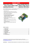
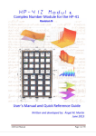
Definition 4. (Z-polyhedron) A Z-polyhedron is the intersection of a polyhedron and an affine integral full dimensional lattice.
A Z-polyhedron can be defined as the image of a polyhedron by an invertible,
integral function. Consider, for instance, the lattice L1 = {2i + 1, 3j + 5 | i, j ∈
Z} and the polyhedron Q1 = {i, j | 0 ≤ i ≤ 5, 0 ≤ 3j ≤ 20}. Then Z1 = L1 ∩ Q1
is a Z-polyhedron (see figure 6.1). Z1 can also be expressed as:
Z1 = {2i + 1, 3j + 5 | − 1 ≤ 2i ≤ 4, −15 ≤ 9j ≤ 5}
,
which is the image of polyhedron Q2 = {i, j| − 1 ≤ 2i ≤ 4, −15 ≤ 9j ≤ 5} by
the function (i, j → 2i + 1, 3j + 5). Q2 is obtained by taking the preimage of
Q1 by the function defining the lattice: (i, j → 2i + 1, 3j + 5).
As Polylib operates on domains made out of unions of polyhedra, it is natural
to define a similar object for Z-polyhedra. A Z-domain is a finite union of
intersections between a domain and a full dimensionnal integral affine lattice.
The set of Z-domains is closed under union, intersection, difference, and image
by integral invertible function.
The image and pre-image by rational functions is also implemented in Polylib,
but the result of the image (or pre-image) is always intersected with the canonical lattice (Z n ). See [NRi00] for further detail on this subject.
27
Figure 6.1: example of polyhedron Q1 = {i, j | 0 ≤ i ≤ 5, 0 ≤ 3j ≤ 20}, lattice
L1 = {2i + 1, 3j + 5 | i, j ∈ Z} and Z-polyhedron Z1 = Q1 ∩ L1 (the dotted line
represent the shape of the original rational polyhedron).
From the implementation point of view, a Z-polyhedron is represented internally as the image of a polyhedron by an affine, invertible mapping. Hence,
storing a Z-polyhedron amounts to storing a domain and a matrix.
6.2
Main functions of Zpolyhedron.c
As for the polyhedra, the function operating on Z-polyhedra are classified depending on whether they operate on Z-polyhedra or Z-domains (unions of Zpolyhedra. However, Z-polyhedra and Z-domains are stored in the same data
structure.
Bool isEmptyZPolyhedron (ZPolyhedron *Zpol): Returns True if ’Zpol’
is empty, False otherwise
ZPolyhedron * ZPolyhedron Alloc (Lattice *Lat, Polyhedron *Poly):
allocate space for a Zpolyhedron structure
void ZDomain Free (ZPolyhedron *Head): free the memory used by the
Z-domain ’Head’
static void ZPolyhedron Free (ZPolyhedron *Zpol): free the memory used
by the Z-polyhderon ’Zpol’
ZPolyhedron * ZDomain Copy (ZPolyhedron *Head): copy a Z-Domain
static ZPolyhedron * ZPolyhedron Copy (ZPolyhedron *A): return a
copy of the Z-polyhedron ’A’
static ZPolyhedron * AddZPolytoZDomain (ZPolyhedron *A, ZPolyhedron *Head): add a Z-polyhedron to a Z-domain performing a check
of inclusion
ZPolyhedron * EmptyZPolyhedron (int dimension): return the empty
Z-polyhedron
Bool ZDomainIncludes (ZPolyhedron *A, ZPolyhedron *B): test the
inclusion of two Z-Domains
Bool ZPolyhedronIncludes (ZPolyhedron *A, ZPolyhedron *B) : test
the inclusion of two Z-polyhedra
28
void ZDomainPrint (FILE *fp, char *format, ZPolyhedron *A): print
the contents of a Z-domain ’A’
static void ZPolyhedronPrint (FILE *fp, char *format, ZPolyhedron
*A): print the contents of a Z-Polyhedron ’A’
ZPolyhedron * ZDomainUnion (ZPolyhedron *A, ZPolyhedron *B):
return the union of two Z-polyhedra domain
ZPolyhedron * ZDomainIntersection (ZPolyhedron *A, ZPolyhedron
*B): return the intersection of two Z-polyhedra domain
ZPolyhedron * ZDomainDifference (ZPolyhedron *A, ZPolyhedron *B):
return the Z-domain difference of the domains ’A’ and ’B’
ZPolyhedron * ZDomainImage (ZPolyhedron *A, Matrix *Func): find
the image of a Z-domain
ZPolyhedron * ZDomainPreimage (ZPolyhedron *A, Matrix *Func):
find the preimage of a Z-domain
ZPolyhedron * ZPolyhedronIntersection (ZPolyhedron *A, ZPolyhedron *B): compute the Z-polyhedra intersection
static ZPolyhedron * ZPolyhedronDifference (ZPolyhedron *A, ZPolyhedron *B): return the difference of the two Z-polyhedra
static ZPolyhedron * ZPolyhedronImage (ZPolyhedron *ZPol, Matrix
*Func): return the image of a Z-polyhedron
static ZPolyhedron * ZPolyhedronPreimage (ZPolyhedron *Zpol, Matrix *G): return the preimage of a Z-polyhedron
void CanonicalForm (ZPolyhedron *Zpol, ZPolyhedron **Result, Matrix **Basis): find the canonical form for a Zpolyhedron
ZPolyhedron * IntegraliseLattice (ZPolyhedron *A) : transform a Zpolyhedron with a non integral Lattice
ZPolyhedron * ZDomainSimplify (ZPolyhedron *ZDom) : return the
simplified representation of the Z-domain ’ZDom’
Note: In all functions taking two Z-domains as input, they should have the
same affine integral lattice.
29
Chapter 7
Parametrized polyhedra
and Ehrhart polynomials
7.1
Theoretical background
In this chapter a class of methods for solving an Ehrhart polynomial, which
gives the exact formula for the number of integer points in the polytope, are
mentioned. These functions are working with special polyhedral structures:
parameterized polyhedron and validity domains. This work was theoretically
developed and then implemented at icps (Strasbourg) [Loe99].
7.1.1
Parameterized polyhedra representation
Polylib manipulates rational polyhedra as seen in the previous chapters. There
are two dual representations of polyhedra: the implicit representation, as a set
of constraints, and the Minkowski representation, as a set of lines, rays and
vertices.
A parameterized polyhedron is defined in the implicit form by a finite number
of inequalities and equalities, the difference from the classical approach being
that the constant part depends linearly on a parameter vector p for both equalities and inequalities:
D(p) = {x ∈ Qn | Ax = A0 p + a,
Bx ≥ B 0 p + b}
with p ∈ Qm
where A is a k × n integer matrix, A0 a k × m integer matrix, a is an integer
k-vector, B is a k 0 × n integer matrix, B 0 a k 0 × m integer matrix and b is an
integer k 0 -vector.
The Minkowski representation, as a set of lines, rays, and vertices, of a
parameterized polyhedron is:
n
o
X
D(p) = x ∈ Qn | x = Lλ + Rµ + V (p)ν, ∀λ, ∀µ ≥ 0, ∀ν ≥ 0,
ν=1
where L is the matrix containing the lines, R the matrix containing the rays,
and V (p) the matrix depending on the parameters p containing the vertices of
the polyhedron.
Polylib includes an algorithm computing the vertices V (p) of a parameterized
polyhedron.
30
7.1.2
Parameterized vertices representation
Each vertex of a parameterized polyhedron is an affine function of the parameters p, defined over a validity domain: each vertex exists only if p is included into
the validity domain associated to this vertex. There are two ways of representing
such a set of parameterized vertices and validity domains:
• as a list of pairs, each one containing a vertex and its validity domain,
• as a list of distinct validity domains, and the complete matrix V (p) associated to each validity domain.
There are two functions computing the parameterized vertices in these two
representations : Polyhedron2Param Vertices and Polyhedron2Param Domain
respectively.
7.1.3
Ehrhart polynomials representation
Ehrhart polynomials associated to each of the distinct validity domains correspond to the number of integer points contained in a parameterized polytope,
when the parameters are integers.
Ehrhart polynomials are pseudo-polynomials, that is to say, polynomials
whose coefficients are periodic numbers. Periodic numbers take different values depending on the rest of the division of the parameters by the period of this
periodic number.
The function Polyhedron Enumerate, returns a list of validity domains and
each corresponding Ehrhart polynomial.
7.2
Main functions in polyparam.c
Polyhedron *PDomainIntersection (Polyhedron *Pol1,Polyhedron *Pol2,unsigned
NbMaxRays): computes the polyhedral intersection and in the case
when the result is of lower dimension, it is discarded from the resulting
polyhedra list.
Polyhedron *PDomainDifference (Polyhedron *Pol1,Polyhedron *Pol2,unsigned
NbMaxRays): computes the polyhedral difference and discard the degenerated polyhedra.
Param Polyhedron *GenParamPolyhedron (Polyhedron *Pol): Create
a parameterized polyhedron with zero parameters..
Polyhedron **Elim Columns (Polyhedron *A,Polyhedron *E,int *p,int
*ref ): Eliminate columns from polyhedron A, using the equalities in polyhedron E.
voidCompute PDomains (Param Domain *PD,int nb domains,int working space): Given parametric domain and number of parametric vertices,
find the vertices that belong to distinct sub-domains.
Param Polyhedron *Polyhedron2Param Vertices (Polyhedron *Din,Polyhedron
*Cin,int working space): Given a polyhedron in combined data and
31
parameters space, a context polyhedron representing the constraints on
the parameter space and a working space size, returns a parametric polyhedron with a list of parametric vertices and their defining domains.
voidParam Vertices Free (Param Vertices *PV): Free the memory allocated to a list of parameterized vertices.
7.3
Main functions and variables in ehrhart.c
char **param name : global variable to print parameter names
enode * new enode (enode type type, int size, int pos): ehrhart polynomial symbolic algebra system
void free evalue refs (evalue *e): release all memory referenced by e
enode * ecopy (enode *e): realize a copy of the enode argument
void print evalue (FILE *DST, evalue *e, char **pname): display an
evalue
void print enode (FILE *DST, enode *p, char **pname): display an
enode
static int eequal (evalue *e1,evalue *e2): verifies the equality between
two enodes
static void reduce evalue (evalue *e): try to reduce an evalue
static void emul (evalue *e1, evalue *e2, evalue *res): multiply two
evalues
void eadd (evalue *e1,evalue *res): add two evalues
void edot (enode *v1, enode *v2, evalue *res) : compute the inner product of two vectors in enode form
static void aep evalue (evalue *e, int *ref ) : transform the references in
a evalues vector, using ref
static void addeliminatedparams evalue (evalue *e,Matrix *CT) : transform a vector of evalues in conformity with a given matrix
int cherche min (Value *min, Polyhedron *D, int pos): find an integer
point contained in polyhedron D
Polyhedron * Polyhedron Preprocess (Polyhedron *D, Value size, unsigned MAXRAYS): find the smallest hypercube of size ’size’ contained
in polyhedron D
Polyhedron *Polyhedron Preprocess2 (Polyhedron *D, Value *size,
Value *lcm, unsigned MAXRAYS): finds a hypercube of size ’size’,
containing polyhedron D
int count points (int pos,Polyhedron *P,Value *context): compute the
integer points enumeration
32
static enode * P Enum (Polyhedron *L, Polyhedron *LQ, Value *context, int pos, int nb param, int dim, Value lcm) : find the pseudo
polynomial representation for integer points
static Value * Scan Vertices (Param Polyhedron *PP, Param Domain
*Q, Matrix *CT) : compute the denominator of parameterized polyhedron
Enumeration * Enumerate NoParameters (Polyhedron *P, Polyhedron
*C, Matrix *CT, Polyhedron *CEq, unsigned MAXRAYS): count
points in a non-parameterized polytope
Polyhedron Enumerate : count points in a polytope. The function returns
a pseudo-polynomial depending on the parameters.
33
Chapter 8
Other tools
This chapter presents auxiliary functions of Polylib: a solver for linear diophantine equations, and functions to compute the Smith Normal Form or Hermite
Normal Form of a matrix.
Linear Diophantine equations
Linear Diophantine equations are linear equations in which only integer solutions
are allowed.
Consider a system of m equations in n variables for which we look for integral
solutions.
A∗x+b=0
A is a m × n matrix and b is a vector of order m.
In the homogeneous space, the equation is M x = 0 where
¸
·
A b
M=
0 1
To solve such a sytems, first the rows of M are rearranged in such a way
that the first rank rows of A are the ones which contribute to the rank. This is
done with:
static void RearrangeMatforSolveDio (Matrix *M) : rearrange the matrix in order to solve a diofantine equation.
Then the function SolveDiophantine for solving the equation can be used.
If a solution exists, the procedure returns rank, otherwise it returns −1.
int SolveDiophantine (Matrix *M, Matrix **U, Vector **X) : solve Diophantine Equations
Generally this functions is used in connection with operations on lattices
because a lattice can be seen as a solution of a Diophantine equation.
34
Smith decomposition
Theorem 2. Smith Decomposition. If A is an n × n non-singular integer
matrix, there exist unimodular matrices U and V such that:
i. U AV = ∆
ii. ∆ is a diagonal matrix with entries δi ∈ Z,
iii. δ1 | δ2 . . . | δn
∆ is unique and is called the Smith normal form of A.
For example, consider the matrix:


1 2 3
M =  −3 2 0 
1 0 0
Its Smith normal

1 0
∆= 0 1
0 0
decomposition is: U M V = ∆ where:




0
1 0 0
1
0  U =  1 0 −1  V =  0
6
2 1 1
0
−1
−1
1

0
3 
−2
In [NRi00], an Affine Smith Normal form has been defined for affine matrices.
The corresponding function in Polylib is:
void AffineSmith (Lattice *A, Lattice **U, Lattice **V, Lattice **Diag)
: compute the Smith normal form of a matrix
Hermite Normal Form
A matrix of full row rank is said to be in Hermite Normal Form if it has
the form [B 0], where B is a nonsingular, lower triangular, nonnegative matrix,
in which each row has a unique maximum entry, which is located at the main
diagonal of B.
Each rational matrix of full row rank can be brought in HNF by a series of
elementary column operations.
The following proposition solve the problem of existence of a normal form
for an affine lattice :
Given a full dimensional affine lattice L, there exists a unique matrix H in
Hermite normal form and a unique vector h such that such that L = L(H) + h,
with the property 0 ≤ hi < Hii ∀i.
The unique affine Hermite form of a lattice is stored in ’H’ and the unimodular matrix corresponding to A = H ∗ U is stored in the matrix ’U’.
Algorithm :
1. Check if the Lattice is Linear or not.
2. If it is not Linear, then Homogenise the Lattice.
3. Call hermite for a matrix.
4. If the Lattice was Homogenised, the HNF H must be Dehomogenised and
also corresponding changes must be made to the Unimodular Matrix U.
35
5. Return.
In Polylib we can find the following functions treating the Hermite Normal
Form:
static int hermite (matrix *H, Matrix *U, Matrix *Q) : compute the
hermite normal form of a matrix H.
void AffineHermite (Lattice *A, Lattice **H, Lattice **U) : find the
HNF for a lattice A.
int FindHermiteBasisofDomain (Polyhedron *A, Matrix *B) : find
the hermite basis of a polyhedron.
36
Chapter 9
Data structures
Data structures of Polylib are defined in the include/polylib directory of the
Polylib hierarchy (file types.h and arithmetique.h. We first present the basic
types and then the structured types (matrices, polyhedra, etc.).
9.1
9.1.1
Basic types
Integer representation
During Polylib computation, it may happen that integer size grow quite fast
(especially when using ehrhart). To avoid overflow, Polylib has adopted a
typing mechanism inherited from the Pips paralllelizer developed in ensmp
(Fontainebleau). This typing mechanism uses a macro called value for representing integer. The file arithmetique.h file defines macros for every usual
operations on integers (for instance: the macro value plus(v1,v2) adds the
two values v1 and v2). At compile time a value will be changed into and int,
long int, long long int or mpz t (the gnu multi-precision data-type for integer) depending on the flags given to the configure script (see chapter 11).
This typing mechanism is important to understand because, when using
the library for a project, one has to use its data structures by including the
polylib.h file, hence if this value macro is not used in the project, the developer has to perform explicit cast between int and values.
9.1.2
Error handling
Polylib use a catch-and-throw mechanism for overflow error that could happen
during execution (this mechanism is also taken from ArithLib). The correct
way tous the TRY, CATCH, UNCATCH, TRHOWand RETHROW macros can be seen by
looking at the code. However, these macros use the longjmp C function which
is not compatible with cygwin, these macro simply correspond to a print out on
the stderr on cygwin plateform.
9.1.3
The saturation matrix
The Saturation matrix is a boolean matrix which has a row for every constraint
and a column for every line or ray. Each element sij in S is defined as follows:
37
½
sij =
0,
1,
if constraint ci is saturated by ray(line) rj , i.e. cTi rj = 0
otherwise, i.e. cTi rj > 0
This saturation matrix is stored in a compact form. The bits in the binary
format of each integer in the stauration matrix stores the information whether
the corresponding constraint is saturated by a ray(line) or not.
Considering the fact that the rows associated with equations are all 0 and
all the column of the saturation matrix associated with lines are also 0 we can
conclude that only the entries associated with inequalities and rays can have 1’s
as well as 0’s.
S
Equations
Inequalities
Lines
0
0
Rays
0
0 or 1
typedef struct {
unsigned int NbRows;
unsigned int NbColumns;
int **p;
int *p_init;
} SatMatrix;
9.2
The homogeneous representation of affine
spaces
Polylib manipulates mixed inhomogeneous system of equations. The terms inhomogeneous stands for the fact that it manipulates objects of an affine space
(not a linear space). To transform the inhomogeneous affine space of dimension
n into an homogeneous vector space of dimension n + 1 we use the following
mapping:
µ
¶
ξx
M : x −→
,
ξ≥0 .
ξ
With this mapping, a system P = {x | Ax = b, Cx ≥ d} in the original
inhomogeneous space is transformed into C = {x̃ | Ãx̃ = 0, C̃ x̃ ≥ 0} where
µ
¶
µ
¶
ξx
C −d
à = (A − b), x̃ =
and C̃ =
.
ξ
0
1
An intuitive representation of this mapping is the following: the set P can be
seen as the intersection of the set C with the hyper-plane defined by the equality
ξ = 1. This transformation has the advantage of simplification in the storage
of the polyhedra (only cones are manipulated, hence only rays and lines are
stored). It also simplifies computations.
In this representation, the vector (ray) (1, 2, 1) in the homogeneous (linear)
space correspond to the vector (vertex) (1, 2) in the affine space and the vector
(ray) (1, 2, 2) in the homogeneous (linear) space correspond to the vector (vertex) ( 21 , 1) in the affine space. Hence, the homogeneous representation allow
to represent rational numbers by using only integers. Finally the vector (ray)
38
(1, 2, 0) in the homogeneous (linear) space correspond to the infinite direction
(ray) (1, 2) in the affine space.
Similarly, any affine
x 7→¶F.x+f
µ transformation
¶
µ
µ
¶is naturally extended to the
ξx
F f
ξx
linear transformation
7→
. Hence, in this system, all
ξ
0 1
ξ
integral affine transformations manipulated in Polylib must have a (0, 0, . . . , 0, 1)
as last row. However, the fact that the last element of this row is not one may be
used for
rational transformation. Consider, for instance, the matrix
µ expressing
¶
1 0
G =
. If we consider this matrix as a representation of an affine
0 2
transformation after mapping M, it represents the following function:
µ
¶
µ
¶ µ
¶
ξx
ξx
2ξ x2
M
G
M−1 x
x −→
−→
=
−→
ξ
2ξ
2ξ
2
µ
¶
1 0
Hence the function represented by
is equivalent to the function rep0 2
¶
µ 1
0
2
resented by:
.
0 1
9.3
Matrices and Polyhedra
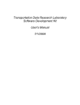
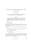
Figure 9.1: Polyhedron structure.
The data types for Vector, Matrix and Polyhedron are the following:
typedef struct {
unsigned Size;
39
Value *p;
} Vector;
typedef struct matrix {
unsigned NbRows, NbColumns;
Value **p;
Value *p_Init;
} Matrix;
typedef struct polyhedron {
unsigned Dimension, NbConstraints, NbRays, NbEq, NbBid;
Value **Constraint;
Value **Ray;
Value *p_Init;
struct polyhedron *next;
} Polyhedron;
The scheme of the polyhedron structure is represented on figure 9.1. Remind
that, in dimension n, each constraints is composed of n + 1 values, the last one
being the constant.
9.4
Lattices and Z-polyhedra
An affine lattice can be represented by an affine matrix. however, we name it
differently because usual operations on matrices normally do not correspond to
operations on lattices (like matrix product for instance). A special data type
has been created for unions of lattices.
typedef Matrix Lattice;
typedef struct LatticeUnion {
Lattice *M;
struct LatticeUnion *next;
} LatticeUnion;
Theoretically a Z-polyhedron can be represented either by the intersection
of a polyhedron and an affine integral full dimensional lattice or by the image
of a polyhedron by an affine integral full dimensional lattice. We choose this
second representation in Polylib. Hence the Zpolyhedron data structure below
represent the image of polyhedron P by the function corresponding to lattice
Lat. The Z-polyhedron represented is the union of all the Z-polyhedra if there
are other Z-polyhedra linked to the next pointer.
typedef struct ZPolyhedron {
Lattice *Lat ;
Polyhedron *P;
struct ZPolyhedron *next;
} ZPolyhedron;
40
9.5
Parametrized Polyhedra
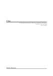
There are two ways of representing the vertices of parameterized polyhedra
(Param Vertices and Param Domain). Both use the same data structure, Param Polyhedron,
described below by the below and shown on figure 9.2.
Figure 9.2: Param polyhedron structure
typedef struct _Param_Poly
{
int
nbV;
Param_Vertices *V;
Param_Domain
*D;
}
Param_Polyhedron;
typedef struct _Param_V
{ struct Param V *next;
Matrix *Vertex;
Matrix *Domain;
}
Param_Vertices;
typedef struct _Param_Domain
{ struct _Param_Domain *next;
Polyhedron *Domain;
int
*F;
} Param_Domain;
41
Chapter 10
Example
This chapter illustrates the use of Polylib by means of a short example. This
example is a C source file which along with polyhedron.c and vector.c does
the following:
• Extraction of a minimal set of constraints from some set of constraints.
• Intersection of two convex polyhedra.
• Application of a linear function to a convex polyhedron.
• Verification that a convex polyhedron is included in some other convex
polyhedron.
These files are compiled together into an executable file called test. When
calling this application the polyhedral domains may be described in two input
files. We are using the file test.in as a sample input data and the file test.out
for the output produced by the program.
This program is shown in Fig. 10.1 and can be used as a pattern for your
own program.
In the following, we detail the different parts of the program. Each instruction of the program is numbered for reference in the following explanation.
Number 1 Read a matrix, for example:
4 4
1
1
1
1
0 1 -1
-1 0 6
0 -1 7
1 0 -2
This is a matrix for the following inequalities:
1
1
1
1
=
=
=
=
inequality, 0x + 1y -1
inequality, -1x + 0y +6
inequality, 0x + -1y +7
inequality, 1x + 0y -2
>=0
>=0
>=0
>=0
-->y
-->x
-->y
-->x
>=
<=
<=
>=
1
6
7
2
Notice that if the first number was a 0 instead of a 1, then that constraint
would be an equality instead of an inequality.
42
#include <stdio.h>
#include <polylib/polylib.h>
int main() {
Matrix *a, *b, *t;
Polyhedron *A, *B, *C, *D;
printf("Polyhedral Library Test\n\n");
a = Matrix_Read(); /* 1 */
b = Matrix_Read(); /* 2 */
A = Constraints2Polyhedron(a, 200);
B = Constraints2Polyhedron(b, 200);
/* 3 */
/* 4 */
Matrix_Free(a); /* 5 */
Matrix_Free(b); /* 6 */
a = Polyhedron2Constraints(A);
b = Polyhedron2Constraints(B);
/* 7 */
/* 8 */
printf("\na =");
Matrix_Print(stdout,P_VALUE_FMT,a);
printf("\nb =");
Matrix_Print(stdout,P_VALUE_FMT,b);
Matrix_Free(a); /* 11 */
Matrix_Free(b); /* 12 */
/* 9 */
/* 10 */
C = DomainIntersection(A, B, 200); /* 13 */
printf("\nC = A and B =");
Polyhedron_Print(stdout,P_VALUE_FMT,C); /* 14 */
t = Matrix_Read(); /* 15 */
D = Polyhedron_Preimage(C, t, 200); /* 16 */
Matrix_Free(t); /* 17 */
printf("\nD = transformed C =");
/* 18 */
Polyhedron_Print(stdout,P_VALUE_FMT,D); /* 19 */
Domain_Free(D); /* 20 */
if (PolyhedronIncludes(A,C))
/* 21 */
printf("\nWe expected A to cover C since C = A intersect B\n");
if (!PolyhedronIncludes(C,B)) /* 22 */
printf("and C does not cover B...\n");
Domain_Free(A);
Domain_Free(B);
Domain_Free(C);
return 0;
}
Figure 10.1: The test.c program
43
Number 2 Read in a second matrix containing a second set of constraints,
for example:
4
1
1
1
1
4
1 0 -1
-1 0 3
0 -1 5
0 1 -2
Number 3 and 4 Convert the constraints to a Polyhedron. This operation
computes the dual ray/vertice form of the system, and eliminates redundant
constraints and reduces them to a minimal form
The 200 parameter is the size of the working space (in terms of number of
rays) that is allocated temporarily and you can enlarge or reduce it as needed.
Number 5,6,11 and 12
Release variables ’a’ and ’b’.
Number 7 to 10 Illustrate how to translate back a polyhedron into a set of
constraints, and print them.
Number 13 Intersect the two polyhedra.
Number 14
itself.
This time, we call Polyhedron Print to look a the polyhedron
Number 15 to 20 Read in a third matrix t containing a transformation
matrix, for example this one that swaps the indices (x, y −→ y, x):
3
0
1
0
3
1 0
0 0
0 1
and take the preimage (transform the equations) of domain C to get D. Print
D, and free it.
Number 21 and 22 Checks the inclusion of A and C, and of C and B.
As a final note: some functions are defined for Domains, others for Polyhedra. A domain is simply a list of polyhedra. Every polyhedron structure has a
”next” pointer used to make a list of polyhedra.
For instance, the union of two disjoint polyhedra is a domain consisting
of two polyhedra. If you want the enclosing convex domain, you have to call
DomainConvex explicity. Note that the inclusion function does not work on
domains, only on simple polyhedra...
The output produced by the program is shown in Fig. 10.2.
44
Polyhedral Library Test
a =4 4
1
0
1
-1
1
0
1
1
1
0
-1
0
-1
6
7
-2
b =4 4
1
1
1
-1
1
0
1
0
0
0
-1
1
-1
3
5
-2
C = A and B =POLYHEDRON Dimension:2
Constraints:4 Equations:0
Constraints 4 4
Inequality: [
1
0
-2 ]
Inequality: [ -1
0
3 ]
Inequality: [
0
-1
5 ]
Inequality: [
0
1
-2 ]
Rays 4 4
Vertex: [
2
5 ]/1
Vertex: [
3
5 ]/1
Vertex: [
2
2 ]/1
Vertex: [
3
2 ]/1
Rays:4
D = transformed C =POLYHEDRON Dimension:2
Constraints:4 Equations:0 Rays:4
Constraints 4 4
Inequality: [
0
1
-2 ]
Inequality: [
0
-1
3 ]
Inequality: [ -1
0
5 ]
Inequality: [
1
0
-2 ]
Rays 4 4
Vertex: [
5
3 ]/1
Vertex: [
5
2 ]/1
Vertex: [
2
2 ]/1
Vertex: [
2
3 ]/1
Lines:0
Lines:0
We expected A to cover C since C = A intersect B
and C does not cover B...
Figure 10.2: The test.c output
45
Chapter 11
Installation
This chapter describes how to install the different parts of the Polylib package.
11.1
Hardware and software requirements
Operating system
Polylib is running on unix-like platform (Solaris, Linux, HPUX) and also on
Windows platforms (provided you have installed cygwin). The Polylib system
will occupy approximately 12MBytes.
Software Requirements
Polylib is built on top of GNU software. In order to install Polylib you will need
the following tools.
• The GNU make command.
• The GNU gcc compiler.
• uncompressing facilities (zcat, gunzip, tar)
On Windows platforms, all these GNU command are available if you install
cygwin: http://www.cygwin.com/.
Polylib may be compiled in 32 bit integer mode, 64 bit integer mode or
arbitrary precision integer mode. This last mode requires the GNU GMP library
(ftp://ftp.gnu.org). Note that this library is not mandatory, you can compile
polylib on 32 or 64 bit mode without having GMP installed.
Documentation is available in the distribution, however, if you want to rebuild documentation files from sources files you will need the Doc++ documentation tool http://docpp.sourceforge.net/ and a Latex Distribution.
11.2
Installation procedure
The Polylib-tree will require about 12 MB of disc space.
Download the polylibX.Y.tgz on http://www.irisa.fr/polylib/
Then type:
46
gunzip polylibX.Y.tgz
tar -xvf polylibX.Y.tar
This will extract the tar file and install all the files in a directory. This
top-directory for the distribution will be named Polylib. This directory will be
called Polylib hereafter. This is how the Polylib-directory will look like after
the extraction:
ArithLib/
Test/
include/
source/
Changes
configure.in
vars.mk
vars.mk.in
Makefile
install-sh
config.guess
config.sub
configure
The installation procedure is based on the configure.in file which checks
for conditions that may change from one system to another, such as the presence
of particular header files or functions. The config.sub and config.guess files are
provided for an auto configuration process. They are used to determine the host
operating system, cpu, etc and put them into a canonical form. The configure
script tries to set system-dependent variables and creates vars.mk which is used
then in the Makefile. It will report what it finds.
The commands that should be typed for installing Polylib and testing its
working are the following.
cd Polylib
./configure
make
make test
make install
By default, the configure script install the 64 bit integer mode, many parameter of the configure script can be changed (see the explanations hereafter).
The make comand already installs the library in order to build the executables. make install installs the documentation, the includes and the binaries.
11.3
Options of the configure script
In fact configure has multiple options. These options allow you to customize
your Polylib installation.
The usage is:
configure
[options] [host]
47
Options: [defaults in brackets after descriptions]
Configuration:
–cache-file=FILE
–help
–no-create
–quiet, –silent
–version
cache test results in FILE
print this message
do not create output files
do not print ‘checking...’ messages
print the version of autoconf that created configure
Directory and file names:
–prefix=PREFIX
–exec-prefix=EPREFIX
–bindir=DIR
–sbindir=DIR
–libexecdir=DIR
–datadir=DIR
–sysconfdir=DIR
–sharedstatedir=DIR
–localstatedir=DIR
–libdir=DIR
–includedir=DIR
–oldincludedir=DIR
–infodir=DIR
–mandir=DIR
–srcdir=DIR
–program-prefix=PREFIX
–program-suffix=SUFFIX
–program-transform-name=PROGRAM
install architecture-independent files
in PREFIX [/usr/local]
install architecture-dependent files
in EPREFIX [same as prefix]
user executables in DIR [EPREFIX/bin]
system admin executables in
DIR [EPREFIX/sbin]
program executables in DIR [EPREFIX/libexec]
read-only architecture-independent data
in DIR [PREFIX/share]
read-only single-machine data
in DIR [PREFIX/etc]
modifiable architecture-independent data
in DIR [PREFIX/com]
modifiable single-machine data
in DIR [PREFIX/var]
object code libraries in DIR [EPREFIX/lib]
C header files in DIR [PREFIX/include]
C header files for non-gcc in DIR [/usr/include]
info documentation in DIR [PREFIX/info]
man documentation in DIR [PREFIX/man]
find the sources in DIR [configure dir or ..]
prepend PREFIX to installed program names
append SUFFIX to installed program names
run sed PROGRAM on installed program names
Host type:
–build=BUILD
–host=HOST
–target=TARGET
configure for building on BUILD [BUILD=HOST]
configure for HOST [guessed]
configure for TARGET [TARGET=HOST]
Features and packages:
–disable-FEATURE
–enable-FEATURE[=ARG]
–with-PACKAGE[=ARG]
–without-PACKAGE
–x-includes=DIR
–x-libraries=DIR
do not include FEATURE (same as –enable-FEATURE=no)
include FEATURE [ARG=yes]
use PACKAGE [ARG=yes]
do not use PACKAGE (same as –with-PACKAGE=no)
X include files are in DIR
X library files are in DIR
48
–enable and –with options recognized:
–enable-int-lib
–enable-longint-lib
–enable-longlongint-lib
–enable-gmpint-lib
–enable-allint-lib
–enable-short-exec
Enable that only an int library is constructed
Enable that only a long int library is constructed (default)
Enable that only a long long int library is constructed
Enable that only a gmp int library is constructed
Enable that 32, 64 and gmp int library is constructed
Enable that the int library is used by the executables
(by default, the long library is used if built)
–enable-extra-suffix
Enable that the executables take an extra suffix depending
on the library size
–enable-all-exec
Enable that the two sized libraries are used to build
two executables of each, which take an extra suffix
depending on the library (by default, only the long library is used)
–enable-onlyshared
Enable that only a shared library is constructed
–enable-onlystatic
Enable that only a static library is constructed
–disable-install-lib
Disable installation of the library
–with-ldconfig-cache=FILE Run ldconfig -C < FILE >
–with-libgmp
DIR Location of the GMP Distribution
You should run ’./configure –enable-gmpint-lib’ to use gmp.
As mentioned earlier you can build the Polylib if you don’t have GMP, but
it will fail when an overflow occurs.
The output of the configure script can be found in vars.mk which is included
by the makefile.
For installing the lib in a private directory you can use the prefix option:
./configure --prefix=MyDir
11.4
Known problems
The configure script does not correctly guess integer size on cygwin platform.
it results in a message during configuration :
checking size of int... 0
... sorry 4
which does not provide any problem (i.e. the size of integer are correctly set by
the script so it is nt a bug).
The cygwin implementation does not correctly work with long long int. It is
apparently due to a bug of cygwin gcc compiler which does not handle correctly
long long int type. Hence, under cygwin, if you do not use gmp you have to
configure in the following way: configure --enable-int-lib
If you try to install the version present under CVS Repository, a possible
error may rise due to the presence of the CVS subdirectory in each directory of
Polylib.
If you install Polylib the tests may fail for long long int library. In this case
you have to use -enable-longint-lib option:
.configure --enable-longint-lib
Notice that the Makefile will try to install the library before building the executables, even when you do not run make install, unless you specify --disable-install-lib
as configure option.
49
Bibliography
[SCH86]
A. Schrijver, Theory of linear and integer programming, John Wiley
and Sons, NY, 1986
[Wil93]
D.K. Wilde, A library for doing polyhedral operations, Technical Report 785, IRISA, Rennes, France, 1993
[NRi00]
S. P. K. Nookala and T. Risset A library for Z-Polyhedral operations,
Technical Report 1330, IRISA, Rennes, France, 2000
[QRR97]
P. Quinton, S. Rajopadhye and T. Risset On manipulating ZPolyhedra Technical Report 1016, IRISA, Rennes, France, 1997
[Loe99]
V. Loechner, A library for Manipulating Parametrized Polyhedra
ICPS RR, March 1999
[Che65]
N.V. Chernikova, An algorithm for finding a general formula for the
non-negative solutions of linear inequalities U.S.S.R. Computational
Mathematics and Mathematical Physics, 5(2):228-133, 1965
[FQ88]
F. Fernandes and P. Quinton. Extemsion of Chernikova’s Alghorithm for Solving General Mixed Linear Programming Problems.
Technical Report 437, IRISA, Rennes, France, 1988
[Le 92]
H. Le Verge, A note on Chernikova’s Algorithm, Technical Report
635, IRISA, Rennes, France, 1992
[CH78]
P. Cousot and N. Halbwachs, Automatic discovery of linear restraints among variables of a program. In Conference Record of the
Fifth Annual ACM Symposium on Principles of Programming Languages, pages 84-96, Tucson, Arizona, 1978. ACM Press.
[MRTT]
T. S. Motzkin and H. Raiffa and G. L. Thompson and R. M. Thrall,
The double description method. In H. W. Kuhn and A. W. Tucker,
editors, Contributions to the Theory of Games - Volume II, number 28 in Annals of Mathematics Studies, pages 51-73. Princeton
University Press, Princeton, New Jersey, 1953.
[ANC]
Corinne Ancourt Génération de code pour multiprocesseurs à
mémoires locales PhD Thesis, France, 1991
50