1
T HE D ELTA
OBJECT TRACKING AND
LOCALIZATION ALGORITHM FOR SENSOR
NETWORKS
Master Thesis
der Philosophisch-naturwissenschaftlichen Fakultät
der Universität Bern
vorgelegt von
Michael Meer
November 2006
Leiter der Arbeit:
Professor Dr. Torsten Braun
Abstract
Wireless sensor networks are an emerging field of research in computer science. Tracking and
localizing mobile objects passing through a sensor network are important tasks for area surveillance in disaster or battle areas. It is a complicated task, because of the need for low reaction
times and cooperation within changing groups of sensor nodes.
We developed the DELTA algorithm to perform both object tracking and localization. It
features dynamic creation of groups tracking objects, requiring no creation and maintenance of
node clusters beforehand. A group leader is responsible for group maintenance, object localization calculations and reporting to the base station. This leader node is not elected randomly
among the nodes, but based on several configurable factors such as strength and tendency of the
sensor readings, interpolated target object position or node battery level. Unlike other tracking
algorithms, DELTA also works when the area where the nodes can sense a target object is bigger than the area within which they can communicate with other sensor nodes. This is mainly
due to an efficient broadcast algorithm spreading leader heartbeats. The leader node performs
localization of the object based on the sensor readings by the leader and at least three neighbour
nodes.
DELTA showed promising results in various tests performed in a network simulator. It was
able to reliably detect and localize target objects and maintain group coherence across a wide
area of parameters.
Contents
1
Introduction
1
2
Related Work
2.1 Object Localization . . . . . . . . . . . . . . . . . . . . . . . . . . . . . . . .
2.1.1 Sensor Network-Based Countersniper System PinPtr . . . . . . . . . .
2.1.2 Sextant . . . . . . . . . . . . . . . . . . . . . . . . . . . . . . . . . .
2.2 Object Tracking . . . . . . . . . . . . . . . . . . . . . . . . . . . . . . . . . .
2.2.1 Efficient Data Aggregation Middleware for Wireless Sensor Networks .
2.2.2 EnviroTrack, an environmentally immersive programming framework
for sensor networks . . . . . . . . . . . . . . . . . . . . . . . . . . . .
2.2.3 Lightweight EnviroSuite . . . . . . . . . . . . . . . . . . . . . . . . .
2.2.4 SensIT project, University of Washington . . . . . . . . . . . . . . . .
2.3 Dynamic Delayed Broadcasting . . . . . . . . . . . . . . . . . . . . . . . . .
2.4 ILA - Intensity-Based Localization Algorithm . . . . . . . . . . . . . . . . . .
3
3
4
5
6
8
9
12
13
15
17
Simulation Environment
3.1 Overview . . . . . . . . . . . . . . . . . . . . . . . . . . .
3.2 OMNeT++ - the Objective Modular Network Testbed in C++
3.2.1 Simple modules . . . . . . . . . . . . . . . . . . . .
3.2.2 Compound modules . . . . . . . . . . . . . . . . .
3.2.3 Network definitions . . . . . . . . . . . . . . . . . .
3.2.4 Running and evaluating a simulation . . . . . . . . .
3.2.5 Other noteworthy features of OMNeT++ . . . . . .
3.3 Mobility Framework . . . . . . . . . . . . . . . . . . . . .
3.3.1 Layers of a mobile node . . . . . . . . . . . . . . .
3.3.2 Mobility models . . . . . . . . . . . . . . . . . . .
3.3.3 Channel control . . . . . . . . . . . . . . . . . . . .
3.4 Own extensions to the simulation environment . . . . . . . .
3.4.1 Simulating a moving target object . . . . . . . . . .
3.4.2 Customized mobility models . . . . . . . . . . . . .
3.4.3 Adapting OMNeT++ vector log files to gnuplot . . .
21
21
21
22
23
24
24
25
25
26
27
28
29
29
31
31
3
iii
.
.
.
.
.
.
.
.
.
.
.
.
.
.
.
.
.
.
.
.
.
.
.
.
.
.
.
.
.
.
.
.
.
.
.
.
.
.
.
.
.
.
.
.
.
.
.
.
.
.
.
.
.
.
.
.
.
.
.
.
.
.
.
.
.
.
.
.
.
.
.
.
.
.
.
.
.
.
.
.
.
.
.
.
.
.
.
.
.
.
.
.
.
.
.
.
.
.
.
.
.
.
.
.
.
.
.
.
.
.
.
.
.
.
.
.
.
.
.
.
.
.
.
.
.
.
.
.
.
.
.
.
.
.
.
.
.
.
.
.
.
.
.
.
.
.
.
.
.
.
4
DELTA, a Distributed Energy-level Based Localization and Tracking Algorithm
4.1 Combination of Localization and Tracking . . . . . . . . . . . . . . . . . . . .
4.2 DELTA configuration . . . . . . . . . . . . . . . . . . . . . . . . . . . . . . .
4.3 Feasibility of Energy Level Based Localization . . . . . . . . . . . . . . . . .
4.4 Operation of DELTA . . . . . . . . . . . . . . . . . . . . . . . . . . . . . . .
4.4.1 Election running state . . . . . . . . . . . . . . . . . . . . . . . . . .
4.4.2 Leader state . . . . . . . . . . . . . . . . . . . . . . . . . . . . . . . .
4.4.3 Member state . . . . . . . . . . . . . . . . . . . . . . . . . . . . . . .
4.4.4 Idle state . . . . . . . . . . . . . . . . . . . . . . . . . . . . . . . . .
4.5 Distributed Election Winner Notification . . . . . . . . . . . . . . . . . . . . .
4.6 Leadership Election Factors . . . . . . . . . . . . . . . . . . . . . . . . . . .
4.7 Preventing multiple leaders . . . . . . . . . . . . . . . . . . . . . . . . . . . .
4.8 ILA - Intensity-Based Localization Algorithm improvements . . . . . . . . . .
37
37
38
39
40
41
43
43
45
45
49
53
55
5
Evaluation
5.1 Evaluation scenario . . . . . . . . . . . . . . . . . . . . . . . .
5.2 Comparison of tracking performance of DELTA and EnviroTrack
5.3 Performance of DENA . . . . . . . . . . . . . . . . . . . . . .
5.4 Localization precision of ILA . . . . . . . . . . . . . . . . . . .
5.5 Continuity of localization . . . . . . . . . . . . . . . . . . . . .
59
59
61
72
78
78
6
Conclusion and future work
.
.
.
.
.
.
.
.
.
.
.
.
.
.
.
.
.
.
.
.
.
.
.
.
.
.
.
.
.
.
.
.
.
.
.
.
.
.
.
.
85
Bibliography
87
iv
Chapter 1
Introduction
Sensor networks and their applications are an emerging field of research in Computer Science.
Composed of hundreds or thousands of tiny battery-powered devices (sensor nodes) equipped
with an array of sensors and a wireless radio to communicate with each other, sensor networks
are utilized to monitor and interact with the environment. Each sensor node should be robust
enough for deployment in hostile environments, low in energy usage to be able to run for several
months or years, and should nonetheless be inexpensive in production. The last goal is not
reached yet, as the current generation of sensor nodes costs around 100 to 200 C. Depending
on the application of a sensor network, sensor nodes may include facilities to sense temperature,
light, pressure, magnetism, sound, motion, chemical substances, GPS signals, etcetera.
There are many obstacles for sensor network applications. Often the sensor nodes are deployed randomly, e.g. dropped from a plane or thrown out of cars, which means the network has
to be able to configure itself and cannot rely on a predefined, static network topology. Battery
capacity is still quite limited and manual recharging is often not possible, therefore conserving
energy is a priority. Nodes might be error-prone, hence consistency checks have to be done.
The possibility of node failures leads to the requirement of redundancy. Radio communication
with other sensor nodes or the base station is expensive (a heuristic rule says 1000 times more
expensive than a calculation operation). Sensing and computing capabilities of single sensor
nodes are limited, making cooperation between several nodes necessary.
Many sensor network deployments require the capability to perform object localization,
meaning to determine the exact location of an event or object within the sensor network’s coverage area. Examples for such events are an outbreak of fire or a leakage of poisonous substance.
Different modalities can be used to localize different types of objects. Measuring the strength of
a magnetic field could be used to estimate the distance of a sensor node to a big metallic object
such as a tank, acoustic shock waves could be used to estimate the distance to an explosion.
An object tracking application has the goal of following a target object moving through the
sensor network’s area, observe certain aspects of the target object and regularly report about
them to the base station. This is complicated by the fact that such an object moves from the
sensor coverage area of certain nodes to the coverage area of other nodes. Tracking applications
might be needed by armed forces to do surveillance in a contested area and follow the path of
enemy vehicles, or keep a watch on endangered animals in national parks.
There are two distinct approaches to perform localization and/or tracking of an event or ob1
ject. In the centralized approach all data are sent from the sensor nodes to a base station, such
as a laptop computer, where all the calculations are done. The main disadvantage of the centralized approach is the big communication overhead, which strains the sensor nodes batteries
and utilizes the limited bandwidth of the sensor network. The distributed approach uses groups
of sensor nodes to perform collaborative signal processing (CSP), resulting in the object’s estimated location. This result is then sent to the base station by a single node in the group, usually
called the leader or the head of the group. The groups are either formed right after the sensor
network has been deployed, or then dynamically just after an event occured. One hurdle for the
distributed approach is the limited processing capability on the single sensor nodes.
Current tracking algorithms (with the exception of SensIt) do not provide proper localization
of the moving object. The result they send to the base station is either the position of the group
leader, which may or may not be the sensor node nearest to the object, or an average of the
positions of all group members.
To be able to track a target object moving through a sensor network reliably and determine
its exact location at the same time, we developed DELTA, the Distributed Energy-level Based
Localization and Tracking Algorithm. Our algorithm uses one or more modalities to detect
an object. A group of sensor nodes is dynamically formed around the object when the object
appears in the sensor networks area. Then a group leader is being elected based on several
user configurable factors such as for example the energy-level of the sensor readings, remaining
power in the node’s battery or distance to the expected path of the object in the future. This
leader informs the nodes in its vicinity about its election, receives the sensor energy-levels of its
one-hop neighbours and uses this information to localize the object with the Intensity-based Localization Algorithm (ILA), provided it has received the information from at least 3 neighbours.
The leader is responsible to inform the base station regularly about the object’s position and to
handover leadership once the object should move out of the leader nodes sensing range.
This master thesis is structured as follows. In the next chapter we provide an overview over
several existing algorithms for object localization and object tracking and describe related work,
done in our research group, that we build upon. In chapter 3 we provide an introduction to the
simulation environment we used to develop and evaluate our algorithm. The environment consists of OMNeT++, a discrete event simulator, and the Mobility Framework, an add-on product
to OMNeT++ to simulate networks with mobile hosts communicating over a wireless channel,
and several additional modules and scripts developed by ourselves. In chapter 4 we discuss
DELTA, our distributed algorithm for object localization and tracking. In chapter 5 we evaluate
DELTAs performance compared with EnviroTrack, an object tracking algorithm developed by
Abdelzaher et al. at the University of Virginia. Chapter 6 presents our conclusions and describes
future work.
2
Chapter 2
Related Work
2.1
Object Localization
Object detection and localization are common features in sensor network applications. The two
main challenges are how to observe potential event locations in a distributed manner and how to
compute the location of an object efficiently and accurately.
Some existing approaches such as [1] use the sensor nodes only to collect data and do the
computation of the event’s location at a base station equipped with more computing resources
and power (such as a laptop computer). This circumvents the limited computing resources at the
individual sensor nodes and the complexity of a distributed algorithm, but accepts the strain on
network bandwidth and sensor node batteries caused by the increased traffic between the nodes
around the event and the base station.
Other approaches observe events through clusters of sensor nodes, that were formed during
the self-configuration [2]. Cluster members are able to directly communicate with the cluster
head and send their information to it. The cluster head collects the data from all the cluster
members and computes the event location. The creation and maintenance of such clusters leads
to communication overhead, especially in wireless sensor networks with nodes being often subject of sudden failure.
Yet another approach is Sextant (see below in chapter 2.1.2), which is a fully distributed
algorithm and does not need a cluster head or base station for computation, but has to disseminate
network and sensor properties in its surroundings.
Other aspects in which localization approaches differ are the kind and number of sensing
modalities used, such as light, magnetism, seismic waves, angle of arrival or time of arrival of
acoustic waves.
With DELTA (see chapter 4) we will introduce a fully distributed algorithm that avoids the
drawbacks of increased communication with a base station and expensive cluster maintenance
and works with sensors for either a single or multiple modalities.
In this section, we will focus on two existing event localization approaches, PinPtr and
Sextant. Object tracking approaches are then discussid in the next section.
3
2.1.1
Sensor Network-Based Countersniper System PinPtr
The Institute for Software Integrated Systems at the Vanderbilt University developed a sensor
network based system to detect and locate shooters in urban environments named PinPtr [1].
This application is in demand of armed forces and law enforcement agencies.
Several sniper detection systems have been developed in the past. Most of these systems
work best in open, flat environments. They struggle to achieve good results in urban terrain
where several complicating factors such as multipath effects or shading effects of the buildings
may occur. Some of the physical phenomena used for sniper detection are:
• Muzzle flash of the weapon, can be detected through an infrared camera and the range
can be estimated through a microphone. It requires direct line of sight, the flash might be
suppressed by the shooter.
• Thermal signature of the bullet in flight.
• Acoustic shock-wave of the bullet travelling at supersonic speed. It is distinctive and
cannot be produced by natural phenomena.
The best results in existing systems have been achieved by employing the time of arrival (TOA)
of muzzle blasts, shock waves or a combination of both. These existing systems are centralized,
using only one or two arrays of microphones. The drawback of this approach is that the localization eventually becomes inaccurate already with a few sensors not detecting the signal; be it
because they are not in the line of sight to the muzzle blast or because the shock wave is shaded
through buildings.
With PinPtr, a system based on a sensor network is introduced as the solution for these
problems. Many sensor nodes distributed over the area of interest increase the chance that several
sensor nodes detect the direct signal and increase the robustness of the system.
The team at the Vanderbilt University implemented and tested a system based on Mica2
Motes sending their TOA information back to a base station, a laptop computer, where a fusion
algorithm calculates the shooters position based on the collected data.
One important prerequisite for successful localization is time synchronization between the
sensor nodes. TOA information of several nodes is used for the fusion algorithm, the more
accurate they are aligned in time, the more accurate the resulting localization can be. For this
implementation the Flooding Time Synchronization Protocol [3] was applied.
Another prerequisite is localization of the sensor nodes themselves. The team experimented
with acoustic localization using the internal sound generator and microphones to localize the
nodes relative to a few anchor nodes. This approach had some limitations such as the range of
the sounder, so the real live tests were done with hand-placed nodes. For this kind of application
it is important to note that the localization periodically has to be repeated, as the enemy might
displace nodes on purpose.
Routing services are very specific to the application, as there is a requirement for a maximum
latency of 2 seconds for the overall system. The TOA information originates from nodes in an
area around the shooter and are generated almost at the same time. PinPtr uses a best-effort,
converge-cast protocol, meaning that the messages are routed to a selected node of the network,
4
called root. Message delivery is not guaranteed, but due to the availability of redundant sensor
readings this requirement can be avoided.
The PinPtr system was tested with 56 nodes placed on an urban warfare training facility of
the US Army. The results are promising, with an average error of the estimated shot location on
the 2 dimensional plane of only 0.6m, for 98% of the shots. The results in 3 dimensional plane
were a little worse with an average error of 1.3m, but this is due to the fact that only few of the
nodes have been placed in elevated positions. Although the performance of PinPtr is already
superior to existing commercial systems, several points have to be improved for successful operations in the field: The sensor nodes have to become more robust and inexpensive, power saving
mechanisms have to be implemented for long deployment periods.
PinPtr has disadvantages compared with DELTA, as it requires centralized computing and
needs measurements of two different phyisical phenomena to perform localization.
2.1.2
Sextant
The Department of Computer Science at the Cornell University developed Sextant [4], a framework to determine the positions of sensor nodes and events in a sensor network. It is able to
determine the position of sensor nodes relative to a number of anchor nodes by solving a system
of geographical constraints. These constraints describe areas where a specific node may be found
(a positive constraint) or where this node definitely cannot be found (a negative constraint). The
wireless radio on each node is used to infer these constraints.
Sextant uses Bézier regions to represent constraints and positions. The advantage of this
approach over a single point representation is that it is able to account for localization errors and
show the whole area where the node, respectively the event, might be located. The advantage
over using a grid of points is a much more compact representation, as only the control points
of the Bézier curves need to be stored and transmitted, and efficient operations such as union,
intersection and subtraction exist.
The few nodes equipped with GPS receivers deliver absolute geographical constraints, as
their position is known exactly. The other nodes provide relative constraints based on their
radio performance and their ability to communicate with their neighbours: if a node A is able to
receive messages of a node B, a positive constraint in form of a circle with radius R around node
A is formed. If node A does not receive messages of node B, a negative constraint is formed
as a circle with radius r around node a. The radius r of the negative constraint is smaller than
the radius R. Determined by measurements with its wireless hardware, node A has to receive
broadcasts of every node within r. Within the larger radius r, it only may receive them, as there
might be coverage holes of the radios.
All Sextant sensor nodes save their sets of constraints locally, there is no central coordination. Each time a node calculates a new estimated location set (the area where the node should
be in, estimated from the set of constraints), it recalculates its assured and its maximal radio
coverage area and broadcasts it as positive respectively negative constraints. Positive constraints
are distributed only to the one-hop neighbours, as only they profit from this information. Negative constraints are distributed over 3 to 4 hops. All constraints are tagged with a validity period,
which is calculated based on the mobility rate of the originating node. Once the validity period
expires, the originating node resends the information.
5
Localizing events works among the same lines as localizing the nodes themselves, required
is only a sensor that can detect if an event occurs or not, a binary sensor. This contrasts with
DELTA, who requires the sensors to return discrete values. Similar as in the case above, the
sensor coverage area has to be examined. The result is the maximum sensor coverage area,
outside of which events cannot be sensed, and the assured sensor coverage area, inside which
all happening events definitely are sensed. After a node A senses an event and waits for a
small amount of time, it broadcasts a event-report request with a certain TTL unless it receives
such a message itself during the waiting time. Other nodes forward the request until the TTL
expires. A node B responds to the request of node A with its estimated location set and either
the maximum sensor coverage area as a positive constraint in case it detected the event too
or its assured sensor coverage area as a negative constraint if it did not. After all responses
are collected, Sextant determines the area where the event happened as the intersection of all
positive constraints minus the union of all negative constraints.
Additionally, through localizing events it is possible to refine the localization of the nodes
themselves. The positive and negative constraints based on the sensor characteristics are exchanged between the nodes and are then also added to the list of radio- respectively GPS-based
constraints used so far for sensor node localization.
Sextant was tested using a setup of 49 Mica2 motes on a 7 × 7 grid with a distance of 61cm
from node to node. The transmission power of the motes was throttled back to 1.5%, leading
to an assured wireless radio range of 121cm and a maximal wireless radio range of 183cm.
A random number of nodes were made anchor nodes and equipped with absolute constraints,
simulating the missing GPS receiver. The localization of more than 90% of the nodes was
accurate when 30% of the nodes where anchor nodes. When feedback of event localization
was used additionally, the mean error of node localization was reduced from 12.2cm to 1.6cm.
Sextant was able to localize 90% of the events within 6cm and all of them within 9cm. It has a
low mean-error and with more nodes its accuracy increases.
2.2
Object Tracking
We define the task of object tracking in wireless sensor networks as being able to observe an
object moving through the network’s area, frequently sending reports about it. Applications of
object tracking are battlefield surveillance, disaster management or protection of endangered
animals in national parks. Object tracking does not include object localization.
A distinction can be done between cooperative and non-cooperative tracking. When the
tracked objects are equipped with means to alert a sensor and identify themselves to the sensor
network, such as an RFID tag, we talk about cooperative tracking. Non-cooperating objects on
the other hand can only be detected through their sensor signatures. The difficulty of associating sensor signatures with a specific object and the mobility of objects lead to non-cooperative
tracking tasks being much more difficult than cooperative tracking tasks. In this thesis, we will
only look at non-cooperative tracking approaches.
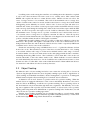
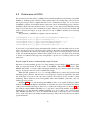
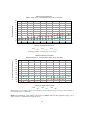
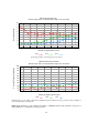
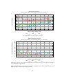
Existing object tracking algorithms can be classified according to several criteria, which
are shown in table 2.2 for the three different algorithms UW-CSP (University of Wisconsin
Collaborative Signal Processing), EnviroTrack and our own DELTA.
6
Table 2.1: Classification of tracking algorithms
Dynamic Groups
Assumption CR > SR
Prediction of object path
Localization
Classification
SensIt
No
Yes
Yes
Yes
Yes
EnviroTrack
Yes
Yes, CR > 2 · SR
No
No
No
Delta
Yes
No, SR < 2 · CR
Yes
Yes
No
The first criterion is the use of dynamically created groups of sensor nodes compared to
predefined clusters. The latter have the disadvantages of being expensive in maintenance as well
as having high overhead when objects are observed by multiple clusters. Dynamic groups on the
other hand might be a bit irresponsive at start when electing a group leader for a newly detected
object, but fit a tracking scenario better as individual nodes may join or leave groups when the
object enters, respectively leaves, their sensor range.
Many algorithms require the assumption that a node’s wireless radio communication range
(CR) is bigger than the sensor range (SR) in which it can detect an object. This assumption
simplifies matters, as all members of a group or cluster are able to communicate directly with
the group / cluster leader and vice versa. Especially algorithms using dynamic creation of groups
benefit: a newly elected leader node can notify all the other nodes sensing a target object about
it’s election with a single message. Later on the leader node can also communicate it’s aliveness
with a single heartbeat message. This simplifies maintaining group coherence.
For real life applications that assumption might not always be fulfilled though. In these
cases, outlying nodes might not hear the leader’s election notification and elect themselves,
leading to the creation of several tracking groups for just one object. In DELTA we are able to
overcome this obstacle through two steps. First, a node might not receive a leader’s broadcast
but the replies of the leaders one-hop neighbours. Upon receiving them, the node might put itself
into a passive mode, not competing for leadership anymore. Secondly, we are able to broadcast
the winner elected message and the following heartbeats efficiently over several hops, accepting
increased latency and bandwidth usage. For each real world application we would need to look
at the physical circumstances and adjust the parameters accordingly.
The SensIt and DELTA algorithms are able to predict the path of the object based on its
past movement and use this information to activate clusters that the object might enter soon
respectively elect group leaders that are crossed by the object in the future. This helps to achieve
a gap less coverage of the object and save energy, as the number of leader elections can be
reduced.
Object localization is a potential additional feature for tracking algorithms, beside SensIT
no other examined algorithm provides it though. What they do report to the base station is either
the position of the group leader or an average of the positions of all group members. Li et al. [5]
already envision localization based on the sensor energy levels, but use different algorithms than
our approach in DELTA.
7
Classification of objects is needed when several objects reside in a sensor networks area
and the tracking application should be able to distinguish between them. Classifiers work on
time-series data of one or several nodes and from one or several modalities, straining the limited
computing resources of sensor nodes and the limited bandwidth of their wireless radios when
transmitting these information. Li et al. [5] are using classifiers to differentiate between wheeled
and tracked vehicles and have some success with their approach. For us, object classification is
an important task and will be investigated in future work.
In this section we will have a closer look at several tracking algorithms that are of interest to
us, but first provide a quick overview over our approach DELTA. As the name of the algorithm
says, we utilize the energy levels returned by our sensors.
DELTA creates dynamic groups and elects the nodes with the highest energy levels to be
leaders of the groups. These leader nodes should be located near to the target object and therefore provide good tracking coverage. The leaders broadcast notification and heartbeat messages,
if necessary DELTA spreads them efficiently over several hops using Distributed Election Notification Algorithm (DENA). DENA is an adapted version of the Dynamic Delayed Broadcasting
(DDB) algorithm that we summarise in Section 2.3. The broadcast over several hops allows us to
get over the assumption that the communication range of the sensor nodes has to be significantly
larger than their sensing range.
Another use of the energy levels is to perform target object localization. One hop neighbours
of a DELTA leader node reply to its heartbeat messages with their current sensor readings. The
sensor readings cannot be taken directly to calculate the distance between a sensor node and a
target object, but in a first stage we can state the ratio of distances of two sensor nodes A and B
to a target object is equal to the inverse ratio of sensor energy leves sensed at both nodes. Our
Intensity-Based Localization Algorithm (ILA) uses data of 4 sensor nodes or more to construct
at least 3 of these ratios. These three equations it puts through a standard least-square approach
to find the location of the target object.
2.2.1
Efficient Data Aggregation Middleware for Wireless Sensor Networks
The Department of Computer Science at the Wayne State University describes an algorithm for
object detection in sensor networks [6] that allows an ad hoc group formation around newly
detected events. As only the group leader has to communicate with the base station and not all
the sensor nodes in the group, energy can be saved. Additionally, every sensor node keeps track
of its probability to gain consensus, meaning a minimum number of other nodes (a quorum)
agreeing with its sensor readings and yielding to it as a leader. When this probability is below a
certain threshold the node is put to sleep temporarily.
Key assumptions for the middleware are:
• Sensing range of a sensor node is entirely contained in its wireless communication range
• The wireless communication range is more than twice as big as the sensing range
• Nodes can determine if they sense the same event
Every node in the sensor network holds a variable with its probability to generate consensus.
Whenever the node is elected as a leader of the group, the variable is increased. Whenever the
8
nodes information contradict with the resulting consensus of the group, the variable is decreased.
If the variable falls below a certain threshold, the node puts itself to sleep for a certain period
and will awake afterwards with a reset probability variable. This is a way to keep faulty nodes
out of the network without rejecting them a chance for rehabilitation.
Whenever a node senses a new event, it schedules a small delay and then, provided no other
node was quicker, starts a consensus generation process by sending out a PROPOSE message.
The initial delay is chosen partly depending on the strength of the sensor readings, partly randomly. The intent to increase the chances for sensor nodes closer to the event to be elected as
leader is based on their higher probability to have neighbours which also sense the event. The
choice of the maximal possible delay is a trade-off, as increasing the delay is limiting communication due to less nodes trying to send concurrently and therefore saving energy, on the other
hand it also increases latency.
As the other nodes receive the PROPOSE message and they agree they sense the same event,
they send back acknowledgements ACK to the initial node, who keeps track of the number of
ACKs it received. Once this number has risen above the parameter QUORUM SIZE, consensus
has been generated and the newly confirmed leader node sends out a DECIDE message to let the
other nodes know.
The parameter QUORUM SIZE has to be selected according to the density of the sensor
nodes. It has to be at least (k + 1)/2 for k nodes inside the region of interest.
2.2.2
EnviroTrack, an environmentally immersive programming framework for
sensor networks
The Department of Computer science of the University of Virginia developed EnviroTrack [17],
a middleware to develop tracking applications for wireless sensor networks. It was implemented
on MICA motes running TinyOS.
EnviroTrack dynamically creates groups (called Context Labels in their terminology) of sensor nodes tracking an event, with one elected leader node responsible for maintaining aggregate
state of the group and running user supplied code to report about or interact with the tracked object. A user has to supply 3 pieces of information to create his own object tracking application:
• A sensee () function that simply returns a binary value if an individual node senses a
specific kind of target object or not. Depending upon the result, a node joins or leaves a
tracking group. An example of a sensing function for detecting a fire is sensef ire () =
(temperature > 180) and (light).
• Definitions of one or more aggregate state variables. Their numeric values are derived by
the group leader node aggregating measurements periodically sent to him by the group
member nodes. A user chooses one of several provided aggregation functions such as
sum, average or barycenter, specifies how fresh the sensor readings must be to be valid
and how many nodes at least must have sent fresh sensor readings for the state variable to
reach critical mass and be valid.
The authors consider it infeasible to maintain exact aggregate state in real time, as communication takes non-zero time and the membership of the groups change fast, that is why
9
they introduce some tolerance with the freshness parameter.
• Tracking objects, meaning functions that will be attached to tracking groups of a specific
kind and can reference the aggregate state variables. In the current version they are run
by the group leader. The functions are run either time-triggered or on arrival of messages
carrying function invocation requests. A typical tracking object might be responsible to
periodically send aggregate state values to a base station.
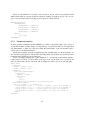
To illustrate the ease of defining a tracking application we present a code example:
(1)
(2)
(3)
(4)
(5)
(6)
(7)
(8)
(9)
(10)
(11)
begin context tracker
activation: magnetic_sensor_reading()
location: avg(position) confidence=2, freshness=1s
begin object reporter
invocation: TIMER(5s)
report_function() {
MySend(pursuer, self.label, location)
}
end
end context
This code snippet defines a tracking object called tracker. The sense function is referenced in
line 2, when a magnetic reading is detected the node would join a group or start a new one. In line
3 the aggregate state variable location is defined as the average of the group member positions,
where the member readings are maximally one second old and at least two valid sensor readings
from distinct sources need to be present for location to be valid. A tracking object reporter is
defined between the lines 5 and 10. Every five seconds it sends the value of the aggregate state
variable location to a node or base station called pursuer.
The group management services of EnviroTrack have two goals. First, they maintain tracking group coherence, meaning that a set of sensor nodes sensing a certain object form only one
tracking group and that the group persists even when the tracked object moves and members of
the group change. Secondly, they maintain the aggregate state of the group.
A leader is elected by the set of nodes sensing a newly appeared target object; as with our
algorithm DELTA the sensor nodes schedule messages to claim leadership with varied delays.
Unlike in DELTA, the delays are just assigned randomly and are not based on any knowledge of
the tracked object or the environment, such as the strength of the sensor readings. EnviroTrack
also splits the period between 0 and the maximal possible delay into discrete slots, increasing
the chances for the messages being sent simultaneously and therefore resulting in collisions.
After its election, the leader of the tracking group sends out periodic heartbeats to inform
group members about its aliveness. Non-member nodes overhearing the heartbeat messages save
the included group identification for a certain period. If these nodes later start sensing the target
object within that period, they join the specified group instead of creating a new one.
Although the authors write in their paper [17] that heartbeats might be spread over several
hops away from the tracking group to inform nearby nodes that a target object might be heading
10
their way, they do not discuss details of how to implement such a broadcast efficiently and do
not implement this feature in their publicly available implementation of EnviroTrack [7]. This
degrades the applicability of EnviroTrack whenever the sensor node radio communication range
is about the same size or smaller than its sensor range. Then, multiple leaders may cover the
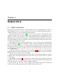
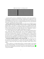
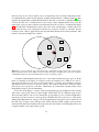
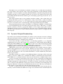
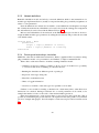
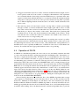
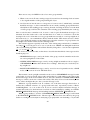
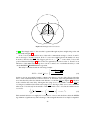
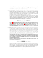
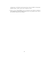
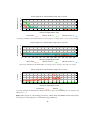
same target object, produce confusion and strain the network’s resources. As indicated in figure
2.1, even when the communication range is the same as the sensing range, a leader will not be
able to inform every node sensing the event that it is elected as a leader or still alive when it
is badly located. This is aggravated by the fact that EnviroTrack elects leaders randomly, thus
leaders located at the fringes are common.
Figure 2.1: A sensor network deployment with radio communication range equal to the sensing range.
The group leader L lies at the fringe of the area where the target object E can be sensed. L is able to
communicate with nodes in less than half the area where sensing is possible.
A situation with multiple leaders may also occur when heartbeat messages get lost. If the
timer of a member node expires as it did not receive any heartbeat for a while, it also tries to
elect itself. Probably it is not able to reach critical mass to start the object tracking operations
and therefore does not report to the base station. If it reaches critical mass, the base station
just receives more reports for some time. Additionaly, if a leader hears another leader, it will
immediately resign to prevent redundancy.
If a node not belonging to or aware of the existing tracking group suddenly becomes a leader
and creates a new group, the base station might assume there are two different target objects
where in reality there is only one. To remedy this, group leaders possess a certain weight that is
increased every time it receives a message from a member and is also passed on to a new leader
during leadership handovers. Group nodes receiving heartbeat messages from two leaders about
the same type of target object will ignore the leader with the smaller weight. If the spurious
leader itself should receive heartbeat messages from the older leader, it will immediately become
a regular member of the older leader’s group.
11
For the evaluation of EnviroTrack, the authors developed a scenario to track Russian tanks
using magnetic sensors. As they did not have any tank at hand, they scaled the scenario down
to a 1000:1 scale and used light sensors already installed on the MICA motes. Later on in the
evaluation of our algorithm DELTA, we will compare both of these algorithms and build some
evaluation scenarios based on this work of Abdelzaher et al. (see Section 5.1). In the scenario
here nodes area arranged in a rectangular grid, with a sensing range of 1 grid-length and a
communication range of 3 grid-lengths. They are able to track a simulated tank travelling with
a speed of simulated 33 km/h, while group coherence degraded when the speed is 50 km/h.
Although the EnviroTrack algorithm also uses dynamic creation of groups as DELTA, it’s
procedure to elect group leaders is quite complicated compared to the latter. Potential leader
nodes in EnviroTrack progress through several stages until one of them reaches leadership.
DELTA nodes in comparison start in ELECTION RUNNING status and then directly switch to
LEADER status respectively MEMBER status, depending on who first notifies the other nodes
claiming its leadership. DELTA necesseraly will produce a leader for the node sooner. In the
evaluation we will see that EnviroTrack indeed has a problem tracking fast moving target objects due to it’s slow election procedures. On the other hand DELTA is prone to elect multiple
leaders at the first appearance of a target object in the sensor network’s area (but resolves these
situations quickly), which is largely avoided by EnviroTrack.
Also EnviroTrack does treat the sensors on its nodes as simple binary sensors, just stating if
there is a target object present or not. DELTA reads the discrete results of the sensors and uses
this information on one hand to elect leaders who are near to the target object and on the other
to perform localization of the target object.
2.2.3
Lightweight EnviroSuite
The authors of EnviroTrack improve its group management services further and propose several enhancements in [8]. Unfortunately at the time of writing this thesis, the source for the
Lightweight EnviroSuite is not published as it is part of a DARPA project. As the paper is not
clarifying several aspects of the proposed algorithm, we compare DELTA in our evaluation with
the publicly available EnviroTrack source to obtain fair results.
The authors identified the dynamic leader election in EnviroTrack, respectively EnviroSuite,
as a bottleneck, hindering better system performance. If the back-off time, the maximal period
a node waits before declaring itself group leader, is too short, multiple nodes might declare
themselves as leader at the same time and create multiple tracking groups for the same target
object. On the other hand, during a longer back-off time fast target objects might already have
moved out of a nodes sensing area before it could be elected and spurious leader would emerge.
They propose 3 measures to improve to existing group management algorithms:
Semi-dynamic leader election
As a high number of sensor nodes participating in the leader election leads to a higher back-off
time to reduce the probability of multiple nodes being elected, the authors propose a mechanism
where only a subset of all nodes are participating in the election phase: the semi-dynamic leader
election.
12
This mechanism requires an initialization phase where some of the nodes are pre-elected to
be leader candidates. The other nodes will not have the possibility to become a leader, unless
they would turn to be leader candidates in a later repetition of the pre-election. Such repetitions
are frequently required, as sensor nodes often pass away and then areas void of any leader
candidates.
The pre-election ideally leads to one node being elected to leader candidate status inside a
radius x. It again uses a random back-off time, with the first node to send out a message being
elected as a leader candidate and the other nodes maximally x away resigning.
We consider this mechanism less than ideal, as it requires frequent maintenance even without
any target objects appearing. A smartly designed back-off function as in DELTA that does not
give every node of the group the same chance to be elected to leadership, but prioritizes nodes
lying near to the target object or fulfill other criteria will not lead to overhead maintenance, but
will still contend with a much shorter back-off time than EnviroTrack.
Piggy-backed heartbeat
The authors saw the possibility to reduce the number of messages being sent in the network by
piggy-backing heartbeat messages on other messages that are anyway sent frequently. One such
item are the reports that a group leader regularly sends to a base station, these are now used
by the Lightweight EnviroSuite as heartbeat messages at the same time. Another item are the
sensor reading messages that group member nodes regularly send to the group leader. They also
have a limited heartbeat functionality now, limited as they are only allowed to repeat heartbeat
messages sent from the leader, but are able to spread the knowledge about an present target
object much farther than if only the leader could notify other nodes.
Implicit leader election
With implicit leader election the authors further decrease protocol costs, provided again there
is continous communication between the group leader and a base station. Nodes usually start
sensing an object at different times due to different distances to the object. Now with an implicit
leader election, every node starts performing leadership duties like data aggregation whenever
they start sensing an object. But as soon as the first sensor node actually sends its data to the
base station, the other nodes will accept this node as a leader for the current cycle and be quiet
until the next cycle starts. The base station thus has the impression of only one group leader
being present. If the sensor node, who was successful with sending its report to the base station
suddenly dies, the other nodes do not notice and just continue doing their leader duties until
another node would reach the end of its cycle and report the results as the first one to the base
station.
2.2.4
SensIT project, University of Washington
In [5] Li et al. describe SensIT, a framework for target tracking, localization and classification.
The algorithms are based on sensing one single modality, such as seismic or acoustic shock
waves.
13
To enable tracking of an object, the sensor network is divided into cells to facilitate local
processing. The size of the cell depends on the velocity of the moving target and the decay
exponent of the sensing modality. Some of the nodes in each cell are designated as manager
nodes for coordinating signal processing and communication in that cell.
Cells are created in the areas where a potential target might enter the Sensor Network, in each
cell several nodes are activated to detect potential targets. These nodes run an energy detection
algorithm sampled at a rate adjusted to the expected targets characteristics.
Tracking a target consists of 5 steps:
1. A target enters cell A. Some or all of the active nodes detect the target. The active nodes
report their energy detector outputs to the manager nodes at N successive time instants.
2. At each time instant, the manager nodes determine the location of the target from the energy detector outputs of the active nodes. The simplest estimate of target location at an
instant is the location of the node with the strongest signal at that instant. More sophisticated localization algorithms justify their higher complexity only if the accuracy of their
location determination is finer than the node spacing. One such algorithm that SensIT
uses is described below.
3. The manager nodes use the calculated locations of the target in the past to predict the
location for a certain period in the future.
4. The predicted target positions are used to create new cells that the target is probably going
to enter.
5. When the target is detected in one of the new cells, this cell takes over as the new active
cell and the nodes in the previous active cell may be put in standby state to conserve
energy.
These steps are repeated for each new active cell. For each detected target, information like
certain past locations are transmitted from the old to the new active cells.
Besides assuming the target location is at the location of the node with the strongest signal
the authors propose a localization algorithm based on energy measurements at multiple nodes. It
combines the measurements of at least 4 nodes and assumes an isotropic exponential attenuation
for the target energy source. It computes the ratios of energy readings of two different nodes
for all the pairs of nodes, then the circles corresponding to the ratios intersect in only one point,
similar to our ILA approach
In case of noisy measurements, more than 4 nodes measurements can be used and the resulting equations are solved using a nonlinear least squares problem. Factors for the accuracy
of this localization method are the preciseness of the node location and the attenuation exponent
measurements. No implementation or detailed sensitivity analysis was conducted by the authors.
Tracking multiple targets complicates matters. If multiple targets sufficiently separated in
space and time exit, so they occupy distinct cells, the same steps as above can be used and a
different track is initiated and maintained for each different target. If the targets lie to close to
each other, classification algorithms are needed.
14
The authors focus on classification conducted on single nodes, as collaborative classification
puts a big burden on the network. They explore the performance of three different classifier
algorithms: k-nearest neighbour classifier, maximum likelihood classifier using Gaussian data
modeling and support vector machine classifier; the test data is real seismic and acoustic data
from tracked and wheeled vehicles with the goal of classifying a given target object into one of
this two classes.
The results with the support vector machine classifier working on the seismic data were
promising. The authors propose two enhancements to improve the results: to either use multiple
modalities in one node at once, or to do collaborative processing between different nodes. In
both cases it is needed to have some knowledge of the target characteristics beforehand.
The group management procedures of SensIT are very different to DELTA’s, as SensIT needs
to create and maintain groups even without any present target objects. This leads to a communication overhead, as well as to groups that might not cover a target object’s path as well as
dynamically created groups with a leader near to the target object. In SensIT it might well happen that a target object moves on the boundary between to groups and does not trigger any alert
in both groups.
2.3
Dynamic Delayed Broadcasting
To perform object localization and tracking in a wireless sensor network, we need to exchange
and spread information inside a certain area of the network. Especially we want to broadcast
leader heartbeat messages to maintain group coherence.
Sensor networks impose specific obstacles to broadcasting algorithms, so as a frequently
changing network topology and a high cost for transmissions. The Dynamic Delayed Broadcasting algorithms (DDB) proposed in [16] addresses these issues. The broadcasting algorithm
is stateless, so it does not need to maintain routing tables or keep track of a node’s frequently
changing neighbors, which would require periodic radio transmissions.
DDB requires sensor nodes to know their geographical positions, which is anyway a requirement for many applications in sensor networks. Whenever a node broadcasts or rebroadcasts a
message in DDB, it stores it’s position in the message header. Other nodes receiving this message use this information as the only external information to decide whether they rebroadcast
the message and when.
The author describes two variations of his DDB algorithms, both trying to deliver a message
reliably to all nodes. DDB 1 tries to minimize the number of transmission in the mean time,
while DDB 2 tries to extend the lifetime of the network. We will focus on DDB 1 in this section.
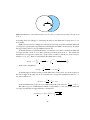
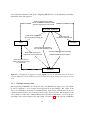
A node A receiving a broadcasted message use the concept of a dynamic forwarding delay
(DFD) and do not forward the received message right away. Instead it calculates the additional
area that a transmission of the message by A would cover, based on the position of the sender
and of A. Based on this additional coverage area, the node A calculates a forwarding delay: the
bigger the additional coverage area, the smaller delay and vice versa. This way, nodes that have
a better chance to reach other nodes will rebroadcast the message first.
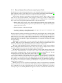
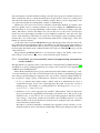
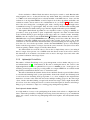
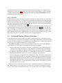
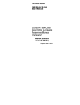
If a node A overhears the message a second time (meaning another node has already rebroadcasted it), it will recalculate the additional coverage area a transmission has and then adjust the
15
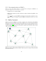
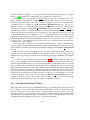
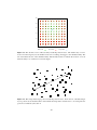
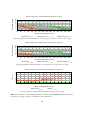
Figure 2.2: Illustration of the additional area a node B could cover when rebroadcasting a message from
node A
forwarding delay accordingly, i.e. increasing the delay as the additional coverage area of A is
now smaller.
DDB nodes may also be configured to rebroadcast a message only if the calculated additional
coverage area is greater than a specified rebroadcasting threshold (RT). Nodes anyway drop their
messages if they cannot cover any additional area at all.
To find the function to calculate the delays, we first have to be able to calculate an additional
coverage area that a node B overs after receiving a broadcast from node A . We assume the
transmission coverage area of all nodes to span a circle of radius 1, and the two nodes to have a
distance of d ∈ [0, 1]. Then we can calculate the additional coverage:
!
Z 1 p
Z −d+1 p
AC(d) = 2 ·
1 − x2 dx −
1 − (x + d)2 dx
− d2
− d2
which can be simplified to:
dp
d
4 − d2 + 2 arcsin ( )
2
2
To find the upper boundary for the possible additional coverage areas, we set the location of
the node B right on the edge of node A’s transmission coverage area and therefore fill in d = 1
into the formula above:
√
3 π
+ ) ' 1.91
ACM AX = (
2
3
AC(d) =
AX
So the maximum area a node can cover additionally with a rebroadcast is ACM
' 61%.
π
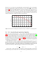
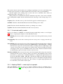
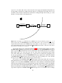
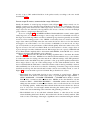
The author proposes a DFD function which is exponential to to the size of the additional
coverage area and takes its upper limit into consideration:
s
AC
e − e 1.91
Add Delay = M ax Delay ·
e−1
16
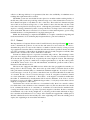
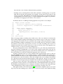
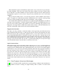
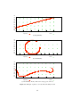
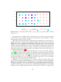
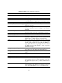
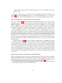
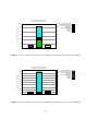
where AC ∈ [0, 1.91] is the size of the additionally covered area and M ax Delay is the parameter for the maximum delay a packet can experience at a node. The function’s curve is shown
in Figure 2.3. Nodes with a higher additional coverage area calculate delay values spread over a
larger interval. This reduces the chance for collisions. Nodes with smaller additional coverage
areas calculate their delays closer to each other. But as they would rebroadcast their transmissions much later, there is a big chance that they will overhear rebroadcasts of other nodes, who
calculated smaller delays, and then cancel their own transmission.
1
Delay
Add-Delay in s
0.8
0.6
0.4
0.2
0
0
0.2
0.4
0.6
0.8
1
1.2
1.4
1.6
1.8
Additional Coverage
Figure 2.3: The dynamic forwarding delay calculated according to the DDB 1 broadcasting algorithm.
2.4
ILA - Intensity-Based Localization Algorithm
Unlike some other existing approaches to object localization like PinPtr (discussed in Section
2.1.1), the Intensity-Based Localization Algorithm (ILA) described by Markus Wälchli [13]
does not need two different kind of sensors to distinguish between two different modalities. On
the other hand ILA is able to make use of the increasing sensitivity of current sensors, and not just
treat them as binary sensors like Sextant (see Section 2.1.2). We will demonstrate the viability
of using sensor intensity levels in Section 4.3. The ILA algorithm is generically computable and
not depending on specific hardware.
One requirement to be able to conduct localization and calculate the position (tx , ty ) of a
target T is any sensor node in the significance area the intensity determining the amplitude of
the target’s signature can be derived. Our assumption is that the intensity ωX sensed at a node
X is related to the distance dX the target is away from X. The farther the target is away, the
lower the sensed intensity is. This relationship is formalized in the following equation:
ωX ∼
1
dαX
with α > 1
(2.1)
The exponent α stands for the degree of attenuation of intensity depending on the distance
between the target object and the sensor node. The formula is generalized and can be used for
17
electromagnetic, acoustic and other path loss models. For magnetism the attenuation is similar
to d13 , for acoustic emissions the attenuation is similar to d12 .
We cannot use the sensed intensity directly to calculate the distance between a sensor node
and the source of the emissions, the target object. Instead we will show that a sensor node A
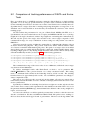
that knows its own intensity ωA and position (ax ,ay ) and also the intensities and positions of at
least three other non-collinear nodes, is able to calculate the position of the target object. The
distance dA of sensor node A from the target object T can be calculated with the theorem of
Pythagoras:
d2A = (ax − tx )2 + (ay − ty )2
(2.2)
From the equations 2.1 and 2.2 we derive the general equation to get the ratio of sensed
intensities of two sensor nodes A and B:
(ax − tx )2 + (ay − ty )2
=
(bx − tx )2 + (by − ty )2
ωB
ωA
2
α
(2.3)
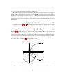
Equation 2.3 says that the ratio of distances of two sensor nodes A and B to the target object
position is equal to the inverse ratio of intensities sensed at both nodes. Unless the ratio is 1, the
equation forms a circle. The case of a ratio equal 1 will be discussed later on. When we form the
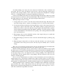
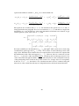
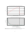
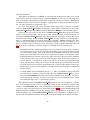
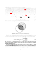
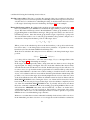
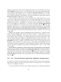
3 ratios between node A and one of the three nodes A, B and C we will get 3 circles. T will lie
on the uniquely determined intersection point of these circles, as long as the sensed intensities
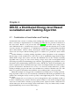
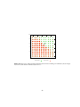
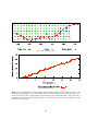
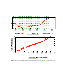
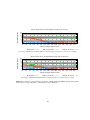
are correct. Please see Figure 2.4 for an illustration of this.
30
20
10
-20
-10
0
x
0
10
20
30
40
50
y
-10
-20
-30
-40
Figure 2.4: Multilateration based on 4 sensor nodes delivering information, forming 3 ratios
18
To prove the applicability of equation 2.3, we have to show that the denominator cannot be
zero. This is trivial, as equation 2.3 also says that the denominator can only become zero if
the sensor node B is positioned exactly at the same place as the target object. We can exclude
this case, as the calculation of the target’s position is trivial when it is exactly at a sensor node’s
position. Consequently, the position of a target object is only calculated if it does not lie precisely
at one of the sensor node’s positions. Only in these cases the denominator cannot be zero.
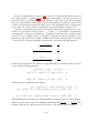
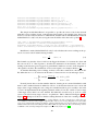
We want to calculate the intersection points of the circles formed through the ratios of intensities of n non-collinear sensor nodes S1 , . . . , Sn with n > 3. To facilitate our calculations,
we change the coordinate system without loss of generality so that the point of origin lies at the
position of node S1 and the x-axis goes through S2 . We will show that the calculation of the
intersection point of the circles is equal to multilateration. In the following equations we write
2 to increase readability. Using the ratios, we get the following equations:
φX instead of ωX
(s3x
t2x + t2y
(s2x − tx )2 + t2y
=
φS2
φS1
t2x + t2y
− tx )2 + (s3y − ty )2
=
φS3
φS1
..
.
(snx
t2x + t2y
− tx )2 + (sny − ty )2
=
φSn
φS1
We dissolve the equations to zero and leave out the denominator, from which we know it cannot
be zero, and get following equations:
φS1 (t2x + t2y ) − φS2 ((S2x − tx )2 + t2y ) = 0
φS1 (t2x + t2y ) − φS3 ((S3x − tx )2 + (S3y − ty )2 ) = 0
..
.
φS1 (t2x + t2y ) − φSn ((Snx − tx )2 + (Sny − ty )2 ) = 0
We transform these equations further and get:
(φS1 − φS2 )t2x + (φS1 − φS2 )t2y + 2φS2 S2x tx − φS2 S22x
(φS1 −
φS3 )t2x
+ (φS1 −
φS3 )t2y
+ 2φS3 (S3x tx + S3y ty ) −
φS3 (S32x
+
S32y )
= 0
= 0
..
.
(φS1 − φSn )t2x + (φS1 − φSn )t2y + 2φSn (Snx tx + Sny ty ) − φSn (Sn2x + Sn2y ) = 0
We can linearize the system above by subtracting the first equation from the rest of the equations.
φ −φ
φ −φ
Therefore the first equation has to be multiplied individually with φSS1 −φSS3 , . . . , φSS1 −φSSn . The
1
2
1
2
resulting equations are subtracted from the second to n-th equation. In all resulting n − 1
19
equations the unknown variables tx and ty are on the left hand side:
2φS3 (S3x tx + S3y ty ) −
2φS2 S2x tx (φS1 − φS3 )
φS1 − φS2
= φS3 (S32x + S32y ) −
φS2 S22X (φs1 − φs3 )
φA − φS2
..
.
2φSn (Snx tx + Sny ty ) −
2φS2 S2x tx (φS1 − φSn )
φS1 − φS2
= φSn (Sn2x + Sn2y ) −
φS2 S22X (φs1 − φsn )
φA − φS2
The equations above indicate that φS1 6= φS2 . We will discuss the special case of φS1 and φS2
being equal in the next paragraph. For now we assume that φS1 6= φS2 and therefore neglect the
denominator as soon as all terms are of the same denominator. If all terms are reordered, we get
a linear equation system of the form Ax = b, with
2(φS3 S3x Γ + φS2 S2x (φS3 − φS1 )) 2φS3 S3y Γ
..
A=
.
2(φSn Snx Γ + φS2 S2x (φSn − φS1 )) 2φSn Sny Γ
φS3 (S32x + S32y )Γ − φS2 S22x (φS1 − φS3 )
..
b=
.
2
2
2
φS3 (S3x + S3y )Γ − φS2 S2x (φS1 − φS3 )
For better readability we substituted here (φS1 −φS2 ) through Γ. This system can be solved using
a standard least-square approach: PT = (AT A)−1 AT B, where P is the estimated position of the
target object. When the inverse matrix cannot be computed, the location cannot be computed and
the multilateration fails. This can happen if φS1 − φS2 . However, this is no restriction as in the
case φS1 − φS2 the ratio of the sensed intensities is 1 and the position of the target object PT lies
on the vertical line through the middle of S1 , S2 . The intersection of this vertical line with any
of the participating circles results in the possible location PT of target object T Consequently,
in the case of φS1 − φS2 , the matrix is not calculated and the location is estimated using the
intersection of the vertical line with any two independent circles derived from the intensities.
20
Chapter 3
Simulation Environment
3.1
Overview
In this chapter we describe the simulation environment we utilized to implement and improve
our DELTA algorithm as well as compare it to our reference algorithm EnviroTrack. The following section is dedicated to the discrete event simulator OMNeT++, why we chose it and
how it functions. The third section describes the Mobility Framework, an add-on to OMNeT++
enabling it to simulate mobile hosts and wireless transmissions. The last section lists our own
extensions to the tools above. They include a simulated mobile target object whose emissions
can be sensed by Mobility Framework hosts, several new mobility modules and a few scripts to
analyze OMNeT++ log files.
3.2
OMNeT++ - the Objective Modular Network Testbed in C++
OMNeT++ [9] is a discrete event simulator developed by András Varga at the Technical University of Budapest, Department of Telecommunications (BME-HIT). Its main application is the
simulation of computer networks, but it is not limited to that domain. The source of OMNeT++
is available under the Academic Public License and it is free to use for academic and noncommercial use.
The main advantages OMNeT++ provides for our work are:
• Good possibilities to debug and evaluate simulation models. OMNeT++ provides a sophisticated graphical user interface to run simulations and interact with them. It also
offers tools to create in real time charts and plots from its logged data.
• Compatibility, OMNeT++ is running under all major operating systems (Windows, Linux,
Mac OS X, other flavors of Unix).
• Strong user-base and community. The mailing list for OMNeT++ is heavily frequented
(typically there are around hundred to two hundred messages each month) and usually
helpful. Additionally there is a wiki where OMNeT++ users share tutorials and frequently
asked questions. This can all be looked up on the OMNeT++ website1 .
1
http://www.omnetpp.org
21
• Expandability. Many simulation models and frameworks have been developed for
OMNeT++ and can be downloaded and applied. Beside the Mobility Framework discussed later in section 3.3, there are for example the INET Framework (containing implementations of the IPv4, IPv6, TCP, UDP protocols and several application models),
NesCT (to run NesC programs from TinyOS on OMNeT++) or OppBSD (an implementation of the FreeBSD network stack).
• Modularity. OMNeT++ is modular on two different levels: First of all when setting up a
simulation different modules implementing the same interface, for example routing modules, can be exchanged in the configuration file for that simulation, without the need to
recompile the simulation. Secondly the OMNeT++ user interface can be expanded by
plug-ins in several aspects, such as new scheduler classes, configuration classes or random number generators.
• Fast prototyping and sophisticated event based modeling paradigm
OMNeT++ simulations consists of hierarchically nested modules. Modules can be simple
modules or compound modules, which consist of sub-modules of either kind. Modules communicate through sending messages either over predefined connections or directly to its destination.
3.2.1
Simple modules
These modules are at the lowest level of the module hierarchy and encapsulate the according
protocol logic. They are written in C++ and are subclasses of cSimpleModule, their definition is
written in a .ned-File. To create customized simple modules, one has to overwrite the following
three functions:
initialize() is called when a new simulation run starts and the network has to be built up. It
may read parameters from the configuration file omnetpp.ini, it initializes custom state
variables and possibly set timers to send the first messages to get the simulation going.
handleMessage(cMessage *msg) is always called when a new message is received at the module, be it through a connection from another module or sent from the module itself (a
self-message, used to implement timers).
Typical functions that might be used within handleMessage() are send() and sendDelayed() to send messages to other modules at once respectively delayed in the future, scheduleAt() to send a self-message to itself at a certain point in the future and
cancelEvent(), to cancel a self-message that was already scheduled with scheduleAt().
finish() is called when a simulation terminates gracefully. Often used to write information to
a log-file. It is not meant to be a replacement for a destructor, as it might not always be
called, so necessary garbage collection might be skipped.
Simple modules may have parameters and gates that are configured in a .ned-File. Gates are
the endpoints of a connection between two nodes, so sending a message from node A to node B
might look like: send(cMessage *msg, cGate *gate);
22
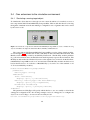
Below a .ned definition of a packet source module is shown, it has a few parameters that
define when and how long the module should keep sending out packets. It has only one outgate, as it is not interested in receiving any message from outside anyway.
simple PPSource
parameters:
sleepTime : numeric,
burstTime : numeric,
sendIaTime : numeric,
msgLength : numeric;
gates:
out: out;
endsimple
3.2.2
Compound modules
To help organize a simulation model OMNeT++ provides compound modules, who consist of
several sub-modules of either simple or compound type. Compound modules do not implement
any functionality on their own, they just bundle the functionality of the sub-modules and so
consist only of a .ned-File definition.
Beside the parameter and gate configuration in the .ned-Files like for simple modules, we
also find there paragraphs for sub-modules (meaning which sub-modules are around and what
parameters they might have) and connections.
In the following paragraph we see the definition of a compound module Mesh, which is
compromised of an array of sub-modules of the type Node. As the name says, it positions the
nodes in a mesh and connects each node with its neighbour on the top, bottom, left and right:
module Mesh
parameters:
height : numeric const,
width : numeric const;
submodules:
node: Node[height*width];
parameters:
address = index;
gatesizes:
in[4],
out[4];
display: "p=,,m,$width,40,40;i=misc/node_vs";
connections nocheck:
for i=0..height-1, j=0..width-1 do
node[i*width+j].out[0] --> node[(i+1)*width+j].in[1] if i!=height-1;
node[i*width+j].in[0] <-- node[(i+1)*width+j].out[1] if i!=height-1;
node[i*width+j].out[2] --> node[i*width+j+1].in[3] if j!=width-1;
node[i*width+j].in[2] <-- node[i*width+j+1].out[3] if j!=width-1;
endfor;
endmodule
23
3.2.3
Network definitions
Runnable simulation models are built by a network definition which is the instantiation of a
module type implemented before (usually a compound module) plus potentially assignments of
values to some parameters.
Network definitions are written also in .ned files, several definitions can find place in a single
file. Usually the desired network definition to be run is chosen in the omnetpp.ini configuration
file. Alternatively it can be selected in the Tkenv GUI (see 3.2.4).
Below a network definition is shown based on the Mesh module type seen before. It tries to
assign the Mesh module types parameters by asking the user directly and provides the user with
some default values.
network mesh : Mesh
parameters:
height = input(9,"Number of rows"),
width = input(7,"Number of columns");
endnetwork
3.2.4
Running and evaluating a simulation
OMNeT++ offers the two different user interfaces: Tkenv, a graphical UI most useful for debugging a simulation model or for presentations, and Cmdenv, a simple command-line UI.
Tkenv offers a rich environment to examine a running simulation model:
• Animation of message sending, possibility to show pop-ups on module icons, possibility
to colorize module icons, formatting of connection arrows
• Running the simulation at different speeds or pausing it
• Inspection of messages being sent
• Time-line of scheduled events
• Charts of logged information
• Overview of variables of the same type in a specified set of modules
Cmdenv is most useful for running a simulation in a batch many times, when direct user
interaction is not needed. During a batch run one or several parameters are be varied, as for
example the number of nodes or the seeds of the random number generators.
Often users might need to create custom charts or plots based on the logged data. This is
possible by transforming the present data into the required format using awk or sed, and then
plot it for example with gnuplot. Several examples of such custom plots can be found in section
5.1.
24
3.2.5
Other noteworthy features of OMNeT++
There are several other features that have to be mentioned in a description of OMNeT++, although they might not have been relevant to our work:
• Graphical editor for .ned-Files GNED
• Support to run simulations parallel on different computers distributed using MPI or other
mechanisms
• Tool opp neddoc to generate HTML documentation from the inline comments in .ned or
.msg files, support for doxygen to generate HTML documentation from the C++ source
files
3.3
Mobility Framework
Without any extension, OMNeT++ is only able to simulate static, wired networks. The Mobility
Framework was written by Marc Löbbers, Daniel Willkomm et al. from the Technische Universität Berlin to add support for node mobility, dynamic connection management and a model of
a wireless channel [10]. Therefore it is well-suited to simulate sensor networks. We use version
1.06a of the Mobility framework.
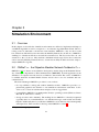
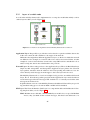
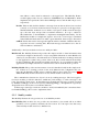
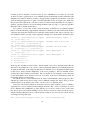
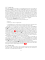
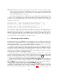
Figure 3.1: Typical simulation using the Mobility Framework. Several nodes are distributed randomly,
the node pairs that are within interference distance with each other are connected. On top left sits the
Channel Control module.
25
3.3.1
Layers of a mobile node
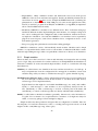
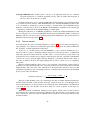
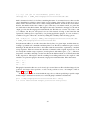
A node in the mobility framework is implemented as a composite module that mainly consists
of three layer modules (see also Figure 3.2):
(a) A mobile node
(b) The NIC Layer
Figure 3.2: A mobile node implemented in the Mobility Framework for Omnet++
Application Layer Responsible to provide the services that in cooperation with the other nodes
in the sensor network will contribute to the targets of the network.
Different nodes might have different Application Layers, as their roles inside the network
are different. One example is a network with a base station and several clients, another
example is a sensor network where several nodes carry GPS receivers and take the role as
anchor to help the other nodes calculate their own positions.
Network Layer Provides routing services to the Application Layer. The stock BasicNetwLayer
simple module encapsulates and decapsulates Application layer packets into Network
layer packets, translates network addresses and corresponding mac addresses, but otherwise directly sends messages from the upper to the lower layer and vice versa.
The Mobility Framework as of version 1.0 alpha 6 only provides one additional Network
Layer, Flood. It broadcasts packets passed from the Application Layer and rebroadcasts
received messages unless the messages TTL reached zero or it already received the same
message from another node.
In planned future versions of the Mobility Framework additional Network Layers providing standard routing protocols such as DSR or AODV will be included.
NIC Layer The Network Interface Card Layer is a compound module and includes the following simple modules (see also Figure 3.2b):
MAC Medium Access Module. The BasicMacLayer module does not provide Medium
Access, they just hand all the received messages, that have been addressed to its
26
mac address or have been broadcasted, to the upper layer. The Mobility Framework though provides also two subclasses CSMAMacLayer and Mac80211, which
implement non-persistent Carrier Sense Multiple Access and the 802.11b protocol,
respectively.
Decider This module decides whether a message from another node has been received
correctly or not. If it was indeed received correctly, it is passed on to the upper layer.
The BasicDecider module does not decide, it just passes all the received messages
up to the next layer and provides convenience functions. It is up to subclasses
like SnrDecider or Decider80211 to implement meaningful functionality. In the
SnrDecider module for example the signal to noise ratio of a message is calculated
in the SnrEval module and if it is under a given threshold, the message is discarded.
snrEval Sends and receives messages through the wireless channel, simulates that messages have non-zero receiving time. Received messages are handed over to the decider for further consideration.
Additionally to the layer modules we have two utility modules:
Blackboard The Mobility Framework provides this simple module to share information that
several layers might be interested in. A layer can publish information on the Blackboard,
other layers can subscribe to that information, be informed whenever it changes and read
it. One application of that is the position of the node, this is an information the mobility
model is publishing. The network layer might subscribe it to do geographical routing, the
application layer might subscribe it to inform a base station about the nodes position.
Mobility Module The position and movement of a node is handled locally in this simple module. If there is no starting position for the node defined in the configuration file omnetpp.ini, the Mobility module selects a random initial position. Below in section 3.3.2
different Mobility models and creation of customized models are discussed.
The communication between two layers is done by sending messages. The basic application layer modules provide the functions sendDown() and sendUp() to send a message to the
lower respectively upper layers. In the higher layer modules this message would be received
by handleLowerMsg(), in the lower layer by handleUpperMsg(). Encapsulation respectively
decapsulation are done by these convenience functions.
Self messages (messages sent from a module to itself) are handled by the convenience function handleSelfMsg(), this is used to implement timers.
3.3.2
Mobility models
The Mobility Framework only provides two stock Mobility models
BasicMobility This module does not provide any movement, it just stands still at an either
specified or if not specified, randomly chosen location. It is the super class that every
other mobility module class has to inherit from.
27
ConstSpeedMobility This module takes a velocity as an argument, then chooses a random
waypoint and travels to it with the specified velocity. Once it reaches that waypoint, it
chooses a new one and moves on again.
For many applications, more sophisticated Mobility models than these are required and have
to be written as a new subclass of the BasicMobility class. The handleSelfMsg() function has
to be overwritten to change the position according to our wish, then call the updatePosition()
method to write the new position on the Blackboard and finally to schedule a new self message
so that after a certain interval the handleSelfMsg() is called again.
During the evaluation of our DELTA algorithm we created four additional Mobility models
for our own purposes, as we needed Mobility models that are predictable (unlike ConstSpeedMobility) and also can move in more realistic patterns than straight lines. We present these new
Mobility models below in Section 3.4.2.
3.3.3
Channel control
As mentioned in the section concerning Omnet (see section 3.2), two modules exchanges messages (mainly) over connections between their gates. These connections are either predefined in
the .ned-Files or added dynamically at run-time.
In the case of a mobile ad-hoc network (MANET) or sensor network simulation it is to
laborious and error prone to manually calculate all pairs of nodes that are able to communicate
with each other and connect them in a .ned file. Due to excessive memory usage in the local
workstation it does not make sense to simply connect all pairs of nodes, especially as the number
of nodes in a sensor network might reach the hundreds or thousands and the radio range of
the nodes is limited. If the nodes might change their position, it turns out to be completely
impossible.
Here the module Channel control comes to our assistance. One instance of this module is
created in our network and will take care of creating connections only between these nodes that
might interfere with each other. The calculation of this interference distance is based on the
parameters transmitter power, wavelength, path-loss coefficient and a threshold for the minimal
receive power and looks like this:
interference distance =
waveLength2 · pMax
16 · π 2 · minReceivePower
α1
Please note that Channel control is connecting nodes that are within maximal interference
distance with each other; at this distance messages send from node A to node B might not be
received and understood correctly anymore at node B, but may still disturb the communication
of node B. It is up to the decider of node B to check for correct reception of messages (see
section 3.3.1).
When the network is initialized, Channel control queries all the nodes for their positions
and computes the connections between the different nodes the first time. It recomputes every
time a node moves (precisely, after the updatePosition() method is called from inside the nodes
mobility module).
28
3.4
3.4.1
Own extensions to the simulation environment
Simulating a moving target object
To simulate the object that moves through our sensor network and has to be tracked, we wrote a
new compound module EventAndMobilityCompoundHost. This module has the task of moving
through the simulated network and emitting a configurable sensor signature that can be sensed
by the sensor nodes.
Figure 3.3: Inside the compound module EventAndMobilityCompoundHost, used to simulate moving
objects. It includes the simple modules BasicEvent, Mobility and Blackboard
The compound module EventAndMobilityCompoundHost consists of three simple modules,
as seen in Figure 3.3: a Blackboard module, a Mobility module and a BasicEvent module. The
Blackboard module is provided by the Mobility Framework. The Mobility module publishes
its position information there, the BasicEvent module frequently requests this information. The
Mobility module makes the simulated object move through the sensor network. In the file EventAndMobilityCompoundHost.ned we do not hard-wire which Mobility module should be used,
but just declare it has to be a subclass of BasicMobility (so it can be one of the standard or one
of our custom Mobility modules):
module EventAndMobilityCompoundHost
parameters:
mobilityType: string;
submodules:
event: BasicEvent;
display: "p=70,70;i=block/star";
mobility: mobilityType like BasicMobility;
display: "p=130,140;i=cogwheel2";
blackboard: Blackboard;
display: "p=130,70;b=25,25;o=black";
endmodule
The parameter mobilityType will specify which subclass to use, we usually set it inside the
omnetpp.ini configuration file. In following example section of omnetpp.ini, we configure the
object to move according to our custom curve mobility model:
basicSim.eventAndMobilityCompoundHost.mobilityType="CurveMobility"
29
basicSim.eventAndMobilityCompoundHost.mobility.x = 100
basicSim.eventAndMobilityCompoundHost.mobility.y = 230
basicSim.eventAndMobilityCompoundHost.mobility.vHost = 15.0
basicSim.eventAndMobilityCompoundHost.mobility.direction = 45
basicSim.eventAndMobilityCompoundHost.mobility.movementArray =
"5 90 15 ; 7 70 15 ;"
basicSim.eventAndMobilityCompoundHost.mobility.updateInterval = 0.2
The simple module BasicEvent is responsible to provide the sensor nodes in the network
with their sensor readings, based on the distance between the nodes and the event. Below we
show how a node creates a reference to a BasicEvent, and then asks it with BasicEvent’s function
defineValueForCoord(Coord) how strong the event should be felt at the node’s position2 .
char *path = "trackingSim.eventAndMobilityCompoundHost.event";
cModule *calleeModule = simulation.moduleByPath(path);
BasicEvent *basicEventModule = check_and_cast< BasicEvent* >(calleeModule);
double sensorReading = basicEventModule->defineValueForCoord(getPosition());
BasicEvent’s method defineValueForCoord(Coord) calculates the sensor readings at the position of a sensor node X with following formula:
wX ∼
1
dαX
for a > 1
(3.1)
The formula says that the object is felt less the bigger the distance dX between the object and
the sensor node X is. The exponent α describes the attenuation of the intensity of the sensor
readings as the distance grows bigger. It is generalized formula for acoustic, electromagnetic or
other path loss models. The attenuation of an acoustic signal is for example similar to d12 .
To simulate fluctuating sensor readings, we have to introduce a random error into this model.
We define the error e to be related to the distance dX between sensor node and target object:
dX
4·arctan SD
Normal(0,
· λ) if dX ≤ SD
π
e=
(3.2)
0
if dX > SD
Normal() means here a random number function, drawing from a normal distribution with
mean 1 and a standard deviation defined as follows: as the distance between sensor node and
target object is approaching the sensor range, the standard deviation grows steadily to the value
λ (set in our implementation through the parameter stddev). For nodes outside of sensor range
of the target object, there is no error defined. We define the error this way, as we do not want
sensor nodes far from any target object to see phantoms. This is illustrated in Figure 3.4a. In
Figure 3.4b, the impact of the error and the resulting fluctuation of the sensor readings is shown.
2
This is a direct method call between modules. Usually OMNeT++ modules communicate by sending messages
over established connections, but for tightly coupled modules, such as sensor nodes polling their sensors a few times
every second, a direct method call is more efficient. A method called directly from other modules has to inform the
simulation kernel about it by itself calling the method Enter Method() right at the start. Else some internal procedures
of OMNeT++, like ownership management, might not work correctly anymore (see [11]).
30
This model is based on the idea that sensor readings are getting more erroneous, the farther away
from the target object they are taken, but that this erroneousness cannot grow indefinitely.
After the regular sensor reading value as well as the error is calculated, these values are
multiplied and sent to the clients: wX · (1 + e)
Other parameters for BasicEvent beside the attenuation exponent α, here in the .ned Definition called pathlossAlpha, and the standard deviation at the edge of the sensing range stddev
are:
frequency How often the event’s position should be logged for evaluation purposes
startTime The time when the BasicEvent should start emitting sensor values
period The time when the BasicEvent should stop emitting sensor values
stopTime The time when the BasicEvent should cease any activity
3.4.2
Customized mobility models
During our evaluation of DELTA, we created following four Mobility models, see also Figure
3.5 for plots of typical path examples for these Mobility models:
CircleMobility Host travels with a certain speed around a circle with specified center point and
radius.
TargetMobility Host travels with a certain speed from a start point to a target point and stops
there.
CurveMobility Host can travel in curves with varying speed. The movement can be configured
in a parameter with instructions in the form 10.0 20.0 5.0 ; 15.0 -45.0 25.0 ; , meaning
that in the first step the host should at time 10.0 be travelling in direction 20.0 degrees with
a speed of 5.0, in the second step the host should at time 15.0 be travelling in direction
-45.0 degrees with a speed of 25.0 Between the states at time 10.0 and 15.0, the mobility
model linearly progresses from the old state to the new state.
FixedCurveMobility Host can travel in curves, the followed path will be always the same independent from the velocity of the host. This is in contrast to CurveMobility, where a faster
speed leads to a wider curve. FixedCurveMobility is configured through instructions in
in the form 45 150 ; 0 300 ; 100 -90 ;, with the first number in each tuple being the
direction the host has to have at the end of that step, the second number being the distance
to be travelled until the end of that step. The velocity is a regular single parameter, the
host will always travel with constant speed.
3.4.3
Adapting OMNeT++ vector log files to gnuplot
Although OMNeT++ offers its own tools to analyse simulation results by visualizing the log
files (Plove and Scalar, [11, Chapter 10]), they did not fit our needs. Firstly we often needed to
31
Error for sensor readings, sensing distance 25, parameter for maximal standard deviation 50%
0.5
0.375
Error
0.25
0.125
0
0
25
Distance sensor node - target object
Fluctuation margin of erroneous sensor readings, sensing distance 25
1
0.875
Sensor reading
0.75
0.625
0.5
0.375
0.25
0.125
0
0
25
Distance sensor node - target object
Sensor reading plus 50% standard deviation of error
Sensor reading minus 50% standard deviation of error
Correct sensor readings
Figure 3.4: Error model for sensor readings. The sensing range in this example is 25 points, the standard
deviation is 0.50. This error of 0.50 can be found exactly at the edge of the sensing range
32
visualize positions and paths of several objects at once, which Plove is not able todo. Secondly
we had to be able to generate plots of our simulation runs automatically from the shell after each
simulation run, whereas in Plove we have to haggle with the graphical user interface every time
again (Loading the right vector log file, select the individual vectors we want to plot, make sure
the plots have the right layout). Last but not least we wanted to have flexibility in our output, to
generate .png files when we are just checking simulation runs for bugs or to generate .pdf files
which we want to include in this thesis.
To log data to a vector file, we first create an instance of cOutVector, set a human readable
name for it in the initialize() stage with the cOutVector.setName(const char *name) method, then
output the data using the cOutVector.record(double value) method. The output of all log vector
in a simulation will be saved in one file (typically omnetpp.vec), which will look similar to this:
vector 16 "basicSim.host[2].appl"
16 0.808116615003 5
vector 14 "basicSim.host[2].appl"
14 0.808116615003 151.475366005
14 0.808116615003 248.353089023
vector 17 "basicSim.host[2].appl"
17 0.808116615003 0.808116615003
vector 20 "basicSim.host[2].appl"
20 0.808116615003 7
vector 13 "basicSim.host[1].appl"
13 1.06068689898 8
20 1.308116615 10
13 1.53953630203 8
20 1.808116615 10
"Generated Event Tags"
1
"Leader Node Positions"
"Leader Elected Time"
"Sent Messages"
1
"Sent Messages"
1
1
1
In the log files we find two kind of lines. The first kind is the vector declaration line, like the
first line in our example above. It consists of the automatically defined vector identification, here
16, then the full name of the simple module that recorded the vector, the human readable name
for this vector, then at last the multiplicity of the vector (usually 1). The second kind of lines
are data lines, they hold the recorded data. The second line in our example is such a data line
for the immediately above declared vector 16. It consists of the vector identification, then the
time-stamp and the recorded value.
We will show how to extract information out of these often hundreds of lines long vector files
and then plot paths and positions using our most difficult example, the target object positions
calculated at the group leader sensor nodes over the course of a simulation run.
After every successful localization, the leader node records the resulting x and y coordinates
separately into a vector named Calculated Target Positions. The x and y coordinates are saved
in two different lines (OMNeT++ provides function to record two values at once on the same
line, but we never succeeded in making it work). First we need now to filter for all the vectors
named Calculated Target Positions, each node had created its own vector before. We do this by
executing following awk script:
awk ’/Calculated Target Positions/ {vectornames[$2]=$2}
33
/ˆ[0-9]/ {if ($1 in vectornames) {print $3}}’
omnetpp.vec > $TMP_DIR/targetpositionscalculated1.dat
Awk is instructed to first look for lines containing the name of our wanted vectors, then save the
vector identification, which is always in the second column of these lines, in the array vectornames. In the next line awk looks for lines starting with numbers, checks if the vector identification, the number in the first column, is part of the array vectornames and if yes, prints the
recorded value in the third column. The input for the awk command is omnetpp.vec, the whole
output goes into the file targetpositionscalculated1.dat. This file now consists only of the x and
y coordinates, but they are still spread over two lines instead of being on the same line and
separated by white-space as expected by our plotting application gnuplot. So now we have to
combine every pair of lines into one line by calling the sed utility with following options:
sed -e’N;s/\n/ /;P;D;’ $TMP_DIR/targetpositionscalculated1.dat
> $TMP_DIR/targetpositionscalculated.dat
Sed (the stream editor) is an editor that takes line by line of a given input, modifies them according to specified user commands and then prints it out. The first command we give sed is N;
meaning it should add the next line to the buffer with the current line, separated by a newline
escape sequence. Then we execute the substitute command s with a regular expression to look
for exactly this newline escape sequence \n and replace it with white-space, s/\n/ /;. Then we
just print it out with P; and jump over the next line in the buffer with D; as we already have that
in the output now. The input is the file resulting from calling awk before, the output is a file
suitable to be plotted in gnuplot afterwards, targetpositionscalculated.dat. It has the format:
120.0 70.0
125.0 68.0
130.0 66.0
The gnuplot instruction files we use obviously plot several data sets like calculated target object
positions, real target object positions or sensor node positions at once. An example of this is
Figure 5.1 on page 63.
To simply plot the file we created with the steps above, without specifying a specific output
format, range considerations etcetera, we could call gnuplot with these instructions:
plot ’/tmp/targetpositionscalculated.dat’ using
1:2 title "Calculated Target positions" with points
34
120
140
160
180
200
220
240
260
280
300
320
100
200
300
400
500
Target path
600
700
Nodes
(a) TargetMobility
140
160
180
200
220
240
260
280
300
320
100
150
200
250
300
350
400
450
Target path
500
550
600
650
Nodes
(b) CircleMobility
140
160
180
200
220
240
260
280
300
320
340
100
200
300
400
Target path
500
600
Nodes
(c) CurveMobility. Clearly visible is the varying speed of the host
Figure 3.5: Example of paths of our customized mobility models
35
700
Chapter 4
DELTA, a Distributed Energy-level Based
Localization and Tracking Algorithm
4.1
Combination of Localization and Tracking
As indicated in the overview on existing object tracking approaches in wireless sensor networks,
there is currently no implementation of a tracking algorithm that also performs localization of
the object itself. Based on our previous the work [12, 13] we use the sensor energy levels
at the individual nodes to calculate target object localizations and show that this does not add
excessive amounts of computation or communication compared to a plain tracking algorithm
such as EnviroTrack. On the contrary, knowing the current and past locations of our target
objects can also help us with the tracking aspect as it enables us to predict the object’s future
path.
Another limitation of existing tracking algorithms is their dependence on the assumption
that the range of radio transmissions of the sensor nodes is significantly bigger than the range
within which a target object can be sensed by the individual sensor nodes. Usually a tracking
algorithm forms a group out of the nodes sensing a target object, with one designated leader
node being responsible for maintaining group coherence, aggregating the group member’s sensor
information and communicating with the base station. The first two duties are facilitated by the
leader’s regular broadcast of heartbeat messages: Nodes receiving them know about the leader’s
presence and aliveness and therefore do not try to be elected as leader themselves, possibly
leading to multiple groups for the same object and therefore confusion. Then the nodes also take
them as a request for information and send their sensor readings back to the group leader.
When this assumption of a bigger radio communication area than sensor coverage area holds,
the group leader’s tasks are easy as it can directly communicate with all the group member nodes
(all the nodes sensing the object) as well as possibly some neighbouring nodes so far not sensing
the object.
If the assumption does not hold up in a real world application, these algorithms would not
be able to maintain group coherence and elect spurious leaders as some nodes sensing the target
object are not aware there is already a group leader present. Spurious leaders confuse the base
station with reports about several target objects where there is only one, unnecessarily consuming bandwidth and power resources while doing so.
37
In the case of Lightweight EnviroSuite, the radio communication range has to be at least
twice as big as the sensor coverage area [8, Section 2.2]. DELTA on the other hand is able to
circumvent this restriction with two approaches:
• When the direct neighbours (or also called one hop neighbours) of the leader node reply
to the heartbeat messages, the leader’s two hop neighbours (able to communicate directly
with the one hop neighbours, but not directly with leader) overhear these. They will
realize that there is a leader present and will remain passive, not trying to elect themselves
to leadership. Using this approach, the assumption can be made more tolerant: the sensing
range may be roughly the same as the radio communication range.
• If the sensing range is found to be bigger than the radio communication range, we have
to spread the heartbeats of the elected leader in the sensor coverage area. Two hop neighbours again overhear the communication of the one hop neighbours and will broadcast
passive heartbeats that can spread out over several hops, configured by the user in the
TTL field. The disadvantage in such a situation is that the leadership election delay must
be higher then to allow the notifying broadcasts to reach all nodes in the sensor coverage
area.
To be able to perform their duties, DELTA nodes need to know their own location information. The nodes may provide this information to DELTA either by GPS receivers incorporated
into the nodes, with the disadvantage of making the nodes bulkier and more power hungry, or by
other approaches using for example a few fixed landmark nodes to calculate the positions of the
rest of the nodes. A survey of localization methods can be found in [15], one method we already
discussed above in Section [4] is Sextant.
DELTA also requires one or several reliable sensors per node to be able to perform precise
object localization and not only object tracking. In the following Section 4.3 an experiment to
prove the feasibility of localization through sensor energy levels will follow.
What DELTA does not require are clocks that are synchronized between all nodes in the
network. The only activity that needs to be synchronized loosely is the periodic saving of sensor
energy levels on the leader node as well as on its one hop neighbours. However, this is already
synchronized through the broadcast of the leader’s heartbeat messages which arrive at the same
time at the neighbour nodes. The propagation delay is small enough to be ignored.
4.2
DELTA configuration
In Table 4.2 we give an overview of the important parameters of the DELTA application layer.
A user planning to deploy a DELTA-equipped sensor network will have to adapt these parameters according to present circumstances in the field. In following list we demonstrate several
environmental aspects and some of the parameters that have to be adapted depending on them:
• Sensor node capabilities
– Radio transmission distance, used to calculate some delays for efficient broadcasting
– Sensing distance, used to calculate some delays for efficient broadcasting
38
– Confidence threshold, used to distinguish real target objects from the noise
– TTL (Time to live) field of heartbeat messages to ensure group coherence in case the
sensing distance is farther than the radio transmission distance
• Sensor network topology
– Maximal Delay for Leader Elected Message, should be higher with high sensor node
density to reduce probability of multiple nodes starting to transmit at the same time
– Maximal Delay Leader IREP Message, should be higher with high sensor node density to reduce probability of multiple nodes starting to transmit at the same time
• Characteristics of the expected target objects
– Heartbeat Delay, should be lower when target object is expected to move fast
– Weights of the different leadership election factors will have to be adapted according
to the speed of the target objects, to the predictability of their paths and to the quality
of the sensors on the nodes. This is discussed in Section 4.6
4.3
Feasibility of Energy Level Based Localization
As no existing localization algorithm uses a combination of energy levels of sensors in different
nodes to calculate an object’s position, we performed a small feasibility study [12] to see if this
approach could lead to satisfying results with current sensor nodes. The potential problems are
the low quality of the sensors, especially fluctuating sensor readings or not calibrated sensors,
as well as physical phenomena such as echo and multipath effects.
For the experiments they utilised a number of Embedded Sensor Boards (ESB) from Scatterweb [14]. These sensor nodes are equipped with a MSP430F149 microcontroller, 2 kilobyte
RAM, 60 kilobyte flash memory, an infrared interface, a timer and a low power consuming
radio. They also are equipped with sensors for luminosity, noise detection, vibration, passive
infrared movement detection and a microphone. The manufacturer claims a lifespan for one
battery charge of 5 years with a duty-cycle of 1% sensing and transmitting or 17 years when
sending 25 bytes every 20 seconds.
The passive infrared motion detection sensor (PIR) was used in the experiments, its sensor
readings were fed to a base station, performing the Intensity-based Localization Algorithm (ILA)
which we also use as part of DELTA and explain later in Section 2.4.
Three different setups for the experiments were created:
1. A small static object (a hand) placed on a table, surrounded by 8 sensor nodes. The object
was positioned at 3 different locations for about 20 seconds each and the average of the
intensities used as input for ILA. The interval was so long as the current PIR sensors
showed a lot of variation. The experiment was conducted 8 times for each of the three
locations, the average distance errors for the locations were 22 cm, 18 cm and 11 cm.
39
2. A bigger, but still static object in a corridor of 5 meters width and 5 meters length, 5 sensor
nodes spread at each side of the corridor on a height of 90 centimeters. The experiment
was conducted with the object being located at the different spots, repeated 8 times each.
Again it could be demonstrated that there is a correlation between the calculated and the
real position of the person, but in one of the spots the variance was big. This is probably
due to different lighting situations inside the same room and/or variant sensitivities from
node to node.
3. The same big object as in the former scenario, moving with a constant speed straight
through a corridor of 4 meters width and 4 meters length, again with 5 sensors on each
side of the corridor. The corridor was reduced in size to increase the density of the nodes,
with the hope to improve the accuracy of the results. The results were promising with
localization errors of only a few dozen centimeters in the middle of the corridors. At the
start and end of the corridor the results were skewed to the middle of the corridor as a
result of lesser sensor coverage at this point.
We conclude that an energy-level based localization on existing sensor nodes is possible,
under certain restrictions. Especially the network density and the location of the sensor nodes
are influencing the accuracy of the location results. They identified the sensing limitations of
the ESB sensor nodes, especially the PIR sensor. Calibration of the sensors could enhance the
accuracy. To use ILA with more appropriate hardware seems to be promising.
4.4
Operation of DELTA
As DELTA is a distributed algorithm, the sensor nodes do not just blindly send their data back
to a base station where the data is getting aggregated into meaningful results. Instead they collaborate to compute the desired results. To achieve this, we assign different roles to the nodes:
one sensor node should be the leader of a group around the tracked object and be responsible
for maintaining group coherence, localization of the target object’s position and communication
with the base station; this node is in the state LEADER. Other sensors sensing the target object
should deliver their information about the object to the group leader, they are in the state MEMBER. Sensors not sensing the tracked object check their sensors regularly in case a target object
suddenly appears and should overhear the communication of other nodes to be warned when a
target object moves into their direction. These sensors are in the state IDLE. Unlike in some
other approaches like SensIT (discussed in Section 2.2.4) where the roles are defined before any
events happen, DELTA assigns roles to the nodes dynamically by electing a group leader and
telling the losers of the election to be group members. During the election phase, the sensor
nodes are in the state ELECTION RUNNING.
In the following subsections we outline the flow of the DELTA algorithm when a target
object appears, by describing the process from the point of view of nodes in all the four different roles. Furthermore in this chapter we will discuss some more advanced topics like the
Distributed Election Winner Notification (DENA) algorithm to broadcast information about a
tracking group farther into the network in an efficient manner, how to deal with multiple leaders
around the same tracking object, the Intensity-based Localization Algorithm (ILA) to perform
40
our localization calculations and about configuring DELTA best to work efficiently and reliably
in different real world situations.
Node stopped sensing object,
sends out REELECTION message,
will save event tag for some time
ELECTION_RUNNING
Node starts sensing and
did not posses event tag yet
Node sends out
notification message first
IDLE
LEADER
Node received notification
from elected LEADER node
Node starts sensing and
did posses event tag already
Received REELECTION message
or
Heartbeat Waiting Timer expired
Node stopped sensing
object, will save event tag
for some time
MEMBER
Figure 4.1: A simplified state diagram for a single DELTA sensor node. The dashed lines show actions
caused by influences from the tracked object, the solid lines show actions caused by messages from other
nodes.
4.4.1
Election running state
In the beginning, all DELTA sensor nodes are in the state IDLE. Every single sensor node checks
its sensors regularly to see if a target object appeared in its surroundings. The output of the
sensors is combined by the function confidenceValue(). If the result of this function is above a
confidence threshold, the sensor node knows that a target object is present. The frequency of the
sensor checks as well as the confidenceThreshold are parameters that have to be set by the user
according to the concrete situation in a deployment, see Section 4.2 for an overview of DELTA’s
41
important parameters.
Although in our simulations of DELTA we only modeled one physical modality to be sensed
by the sensor nodes, it would be trivial to implement DELTA on real sensor nodes using more
than one modalities. The benefit would be improved precision and error resilience. The function
confidenceValue() would need to be changed to aggregate the readings of the different sensors
into one value, probably by using fuzzy logics.
As soon as an exemplary sensor node A learned about a target object’s existence, it switches
to the mode ELECTION RUNNING and schedules a timer with a certain delay, to send a NOTIFICATION IREQ message (IREQ stands for Information REQuest) after the timer expires.
If node A does not receive another node’s NOTIFICATION IREQ message before its timer
expires, it elects itself as leader of the group of nodes sensing the target object and starts broadcasting the NOTIFICATION IREQ message. The calculation of the delay between the start of
the election and sending out the NOTIFICATION IREQ message is therefore extremely important, as it will define which node will be elected for leadership. DELTA calculates this delay
based on several leadership election factors including strengths of the sensor readings or proximity to a future location of the target object, these factors will be explained in depth in Section
4.6. Node A has to initialize some state variables concerning the newly formed group:
• An unique event tag to identify the tracked object, respectively the node group covering it,
is created by node A. It is used to announce the tracking group to the base station as well
as to nodes in the vicinity of the group. This event tag remains constant from the time the
target object enters until it leaves the sensor network’s area again, surviving the frequent
leadership handovers between sensor nodes. The event tag is spread over the boundaries
of the area where the nodes sensors can sense the target object. If the target object moves
into the direction of an idle node Q, this node will at some point start sensing the target
object, but instead of starting a new election it will join the group identified by the event
tag. If the target object should not appear in the node’s sensing range and also no messages
mentioning its group are overheard, the node will erase the event tag after a configurable
amount of time.
• A round number will be initialized and set to 1. This round number will be increased
every time before a leader of the group sends out a new NOTIFICATION IREQ or one of
the periodic HEARTBEAT messages and it will be included in the message . All sensor
nodes in the group receiving one of these messages use its round number value to check
if incoming messages are too old and can be ignored.
Through the broadcasted NOTIFICATION IREQ message, the direct neighbours of leader
node A are informed about its election to leadership, therefore they cancel their own timers and
switch to status MEMBER. How to inform neighbours outside the radio communication range
of node A of the successful election is discussed in Section 4.5 about the Distributed Election
Winner Notification (DENA), how far the message will be spread depends on the time to live
(TTL) field that is part of the NOTIFICATION IREQ message. The value is configured also by
the user and will determine until how many hops far away the neighbours should be informed.
42
4.4.2
Leader state
After a node A was elected to be leader of a group tracking the target object, it starts sending out
periodic HEARTBEAT messages (driven by a heartBeatTimer with a user configurable delay).
Their purpose is manifold: they inform the group members that the leader node is still alive,
an important aspect in wireless sensor network with nodes often dying of external damage or
lack of power. Furthermore, they intend to request replies containing the current sensor readings
from the direct neighbours. This information is used for localizing the target object. One nice
side effect of using the heartbeats is that because of them we do not need to synchronized every
node’s clock. One of the physical attributes of a wireless channel is that broadcasts arrive everywhere at the same time, therefore the nodes can save their sensor readings at the moment of the
broadcast’s reception. The propagation delay over such a distance is negligible.
The content of the HEARTBEAT messages consists of:
• Round number, increased by one for every new heartbeat cycle
• Event tag
• TTL field, set to the user configured value
• calculatedTargetPosition, optional field to inform the nodes about the calculated position
after the last heartbeat cycle. If it could not be calculated, this field is empty
If the TTL is set to be larger than one, group member nodes will reply with NOTIFICATION IREP messages containing their sensor readings. The messages are saved in an array.
After at least 3 of them have been received, plus the sensor readings of node A itself, the localization algorithm can be started. How the localization based on the sensor readings work is
explained later in Section 2.4. When the heartBeatTimer triggers a new heartbeat, the node also
resets the array with the saved NOTIFICATION IREP messages, increases the round number by
one, puts the last calculated target object position on top of the stack with the last few calculated
target positions (or a NULL, if there was no successful localization in the last heartbeat cycle).
If the TTL is set to be one, group members are not allowed to reply and we would have a
plain tracking algorithm without any object localization functionality.
Another duty of a LEADER node A is to ensure an ordered handover of leadership once
node A does not sense the target object anymore. A will realize the disappearance of the target
object quickly, as the node continues to poll its sensors. It will immediately send out a LEADERSHIP REELECTION message to its neighbours and then switch to IDLE status. Additionaly
it save the group tag for some time to be prepared if the target object should return.
Upon reception of a LEADERSHIP REELECTION message, member nodes will start electing a new leader while keeping the state of the group like the event tag and the round number
intact. This procedure is explained further in the Section 4.4.3.
4.4.3
Member state
The duties of group member nodes are: reply to information requests from the leader with the
current sensor values, spread periodic leader heartbeats to farther away nodes and detect if a
leader died, to start a leader reelection in that case.
43
There are two ways for DELTA nodes to become a group member:
1. When a sensor node B starts sensing a target object and loses the ensuing election, it turns
to be a regular member of the group tracking the object
2. An object moves into the sensor coverage area of a sensor node C, which lately overheard
heartbeat messages or other communication from a nearby tracking group and therefore
already knows the tracking group’s event tag. Instead of starting an election to be the head
of a new group, it will become a member of the existing group identified by the event tag.
Once a node becomes a member node, it starts to wait for periodic heartbeat messages to be
informed about the leader node’s state and that there is no need for a reelection. From the
description above it is clear that not every group member necessarily is a one hop neighbour of
the leader node, i.e. can communicate directly with the leader. This means we have to find a
way to periodically inform these nodes farther away about the existence of a group leader, else
they might start a leader reelection with confusing results.
This situation appears especially as the ratio of the sensing range and wireless communicaSR
tion range CR
of a node gets closer to one or even above it. DELTA can distinguish itself from
other object tracking algorithms such as EnviroTrack by being able to overcome the requirement
SR
1
SR
CR < 1 or even CR < 2 .
To show how we achieve that, we first have to describe the three kinds of messages used for
heartbeat purposes:
• HEARTBEAT messages, sent by the leader of the group, received at member nodes who
are one hop neighbours of the leader
• NOTIFICATION IREP messages, sent by one hop neighbour member nodes as a reply to
a HEARTBEAT, includes their current sensor readings. Obviously also received by two
hop neighbours
• PASSIVE HEARTBEAT messages, sent by second or more hop member nodes or IDLE
nodes, will be sent as far as its TTL field allows.
The moment a one hop neighbour member node receives a HEARTBEAT message from the
group leader, it saves its current sensor values and updates its round number to the value in the
received message. If the received TTL allows it, the node schedules a NOTIFICATION IREP
message to send its saved sensor values with a delay. This delay is based on the intensity of the
sensor values: the higher they are, the sooner the message is sent.
Whenever a group member node B overhears one of the three messages listed above, it
realizes the continued existence of a group leader and starts, respectively restarts, a HeartbeatWaitingTimer. As soon as this node B does not receive anymore heartbeat message, it
assumes the leader to be dead and starts a reelection of the leadership by sending out a LEADERSHIP REELECTION message and switching itself into ELECTION RUNNING mode.
When a group member C receives a LEADERSHIP REELECTION message, it will switch
to the ELECTION RUNNING mode. The message could have been sent either by the group
leader not sensing the event anymore and trying to properly hand over leadership, or by another
44
group member node that first assumed the leader dead. The ensuing election happens just as
described above in Section 4.4.1, with one exception: the node that finally is elected continues
to use the old event tag instead of creating a new one and bases its future HEARTBEAT messages
on the increased old round number.
4.4.4
Idle state
As idle nodes do not sense any target object, they only have two duties: first to be prepared for
a target object moving into its coverage area by overhearing communication from nodes that are
aware of a present target object. Second, to spread these messages about the object further. The
latter duty is performed through the Distributed Election Winner Notification algorithm (DENA)
and will be explained below in the Section 4.5.
To be aware of a present target object in the sensor network without sensing it, means overhearing heartbeat messages (from the different kinds listed in Section 4.4.3) and save the message’s event tag for a specified time. If a target object appears within this period, the idle node
assumes it is the target object identified by the event tag. If no target object appers in the node’s
range within this period and no further heartbeat messages were received, the event tag is reset.
The length of the period is specified by the parameter resetEventTagDelay.
4.5
Distributed Election Winner Notification
As already mentioned, current tracking algorithms assume that the radio communication range
of a sensor node is considerably bigger than the sensing range, within which a target object can
be observed. If this assumption is not fulfilled, these algorithms start to produce reports about
several target objects where in reality only one can be found.
The DELTA algorithm does not require this arbitrary assumption to be true when DELTA is
deployed in real world. We have two mechanisms in place that can help us:
• If the sensing range is just little less than the communication range, DELTA helps preventing spurious leaders through second hop neighbours overhearing the communication
between one hop neighbours and the leader node, thus realizing the presence of a leader.
So whenever a message is received by a second neighbour, the node resets its heartbeatWaitingTimer and then is passive (i.e. it does not attempt to start a reelection).
• If the sensing range is bigger than the communication range, the leader heartbeats will
have to be spread frequently over several hops to make sure all group member nodes not in
direct contact with the group leader yield to the leader. The DELTA user has to configure
the initial TTL field according to the physical conditions and the expected network density
in the deployment area to be sure the heartbeats will be spread over the entire area where
the target object can be sensed.
In this section we explain the latter point, how to spread the heartbeats over multiple hops.
A flooding broadcast over several hops in a wireless sensor network is an expensive operation
as every sensor node rebroadcasts the message over its radio and receives unnecessary many
45
copies of it. To reduce this strain on the network load we apply the Dynamic Delayed Broadcast algorithm. It prioritizes sending messages that are covering bigger areas that were not yet
touched by the broadcast transmissions and cancels sending messages that would go to areas
already covered by other nodes transmissions.
E
1) HEARTBEAT
L
1h
2) IREP
2h
3) PASSIVE
HEARTBEAT
I
SR
> 1. A
Figure 4.2: An example of communication in a DELTA sensor network with the property CR
leader node L sends out a HEARTBEAT message with a TTL value of 3. It is received only by a one hop
neighbour 1h, which replies with an IREP message with a TTL of 2. This message is overheard by the
group member 2h, which will send out a PASSIVE HEARTBEAT with TTL 1. The idle node I will not
rebroadcast it as the TTL does not allow it.
A typical broadcast cycle as illustrated in Figure 4.2 starts with the leader sending out either a
NOTIFICATION IREQ message if the node was just elected or else a HEARTBEAT message, in
either case the message includes the current round number and the TTL value the user specified.
With a TTL value of 2, only nodes up to the two hops away are informed about the leader
node, with a TTL value of 4 all neighbors up to 4 hops away etc. The first hop neighbors who
are also group members receive the HEARTBEAT message, update their round and schedule
a NOTIFICATION IREP message, the more intense the sensor readings, the sooner will the
message be sent. The TTL value of the message is decreased by 1.
One receiver of the NOTIFICATION IREP messages is the group leader, who uses the included information for its localization duties. The other receivers are obviously the second hop
neighbors, who can either be MEMBER or IDLE nodes. They check the round number included
in the message and discard it if it is smaller than the current round number in the node. Member
nodes then restart their heartbeatWaitingTimers, while idle nodes restart their resetEventTagTimers. If indicated by the TTL number, they schedule to send a PASSIVE HEARTBEAT message which compared to NOTIFICATION IREP messages does not contain the sensor readings
46
as the node cannot communicate with the leader node anyway.
The delay after which a node C broadcasts the PASSIVE HEARTBEAT message is calculated by a DFD mechanism, as described in the Section 2.3. Initially upon reception of the
first NOTIFICATION IREP or PASSIVE HEARTBEAT message of a new round, node C will
schedule its PASSIVE HEARTBEAT message based on the area additionally covered by it sending out the message. For that purpose, we first calculate the area covered by both sensor nodes
as in Equation 4.1, calculated as the intersection of the circles around the node location with
the radius of the radio range, and then the additional coverage area AC+ by subtracting this
intersection from the area covered by our node C in equation 4.2:
AC ∩ A1 = r2 · (2 · arccos(
d
d
) − sin(2 · arccos(
)))
2·r
2·r
AC+ = π · r2 − (AC ∩ A1 )
(4.1)
(4.2)
where r is the radio coverage radius, d the distance between the two nodes.
Figure 4.3: Illustration of terms used in calculating delays
Based on AC+ and the maximal possible additional coverage area AM AX+ (when the two
nodes lie exactly on the edge of each others radio coverage range), we can calculate a delay:
v
u
AC
+
u
t e − e AM AX+
(4.3)
DF D = M AX Delay ·
e−1
The reason to use an exponential function is to prioritize sensor nodes with a bigger additional coverage area and to minimize collisions when these sensor nodes broadcast their PASSIVE HEARTBEAT messages.
If a message of the same round arrives at node C before it could broadcasts its already
scheduled PASSIVE HEARTBEAT message, the added coverage is recalculated and the timer
adjusted as obviously a broadcast from node C now covers less untouched area and its importance decreased. For the recalculation of the delay, we apply the triangle heuristic rule introduced
47
Figure 4.4: Triangle rule for broadcast
in [13]. The triangle refers to the area that is spanned through any three neighboring nodes and
is illustrated in Figure 4.4.
Node C lies in the intersection area of the radio communication ranges of node A and B,
whose messages C already received. Node C covers more additional
area the farther it is away
√
from the connection line AB. The biggest gain AM AX = 43 · r2 occurs when C lies at the
position illustrated in Figure 4.4. We use the area spanned by the sensor nodes A, B and C as an
indication of the additional coverage area of node C and use it to recalculate the delay to send
out the PASSIVE HEARTBEAT message with.
The delay is calculated with the following formula:
v
u
AT riangle
ABC
u
t e − e AT riangleM AX
DF D = M AX Delay ·
(4.4)
e−1
Again we use an exponential formula to enhance the chances of nodes with a bigger triangular
area to send out their heartbeats without collisions. A drawback of the triangular heuristic is the
error introduced by all nodes with the same distance h to the line AB (see Figure 4.4). All these
nodes calculate the same delay, although nodes lying close to the middle of the line AB are
covering more additional area than nodes lying close to the edges. This error is at its maximum
when node C lies directly in the middle of line AB: in this case h is 0, but the additional area
covered is:
"Z r
#
Z rp
2 p
4
r2 − x2 dx −
r2 − x2 dx ∼ 0.22 · r2 π
(4.5)
0
r
2
This maximal deviation of roughly 2% is tolerable for our uses and should not affect the DELTA
algorithm in a significant way. The advantage of the triangular heuristic is its simple computabil48
ity and low memory demand, i. e. compared to the Dynamic Delayed Broadcast in its original
form (see [16]) which tries to calculate the precise additional coverage areas.
If a third message D (or even more messages after that) of the same round arrives, the sensor
node C checks if it lies inside the triangle ABD, formed by the nodes whose messages node C
already received. This check if the node is inside the triangle is easily done using barycentric
coordinates. If it is, C cancels its scheduled PASSIVE HEARTBEAT message. If it is not, C
adds it to the array of received heartbeat messages and continues to listen for other heartbeat
messages and waiting for the PASSIVE HEARTBEAT message send timer to expire. Now as a
fourth message E arrives, C checks again if it is lying inside the triangles ABE or BDE. We
will not check every possible choice of two messagesout of the already received ones, as for the
triangles. Instead we just linearly test the
x−th overheard message we would have to test x−1
2
triangle the sender of the newest message spans with the first and second, then second and third,
then third and fourth etc. This way the number of our tests grow much slower, just x − 2 tests to
be done for the x−th overheard message, but still we cover a considerable amount of the areas
covered by all possible triangles.
Once sensor node C either sent or canceled its scheduled message, C ignores other heartbeat
messages until a heartbeat message with a newer, higher round number arrives. Then we clear the
array with the received messages and start again with scheduling a new PASSIVE HEARTBEAT
message.
That C already receives a heartbeat message of a new round while it did not yet send its
scheduled one may be possible if DELTA is misconfigured. In this case it also just cancels the
scheduled message, the array with the received messages and starts scheduling the heartbeat
again.
As one can see in an exemplary situation in Figure 4.5, the triangle heuristic works quite
well to prevent sending of unnecessary heartbeats. In this example, a new event enters the sensor
network where the TTL being set to 3. A flooding algorithm (i.e. individual nodes not repeating
already sent messages) would have sent messages from 23 different idle sensor nodes. In the
figure, the turquoise nodes up to the fourth column received a notification directly from the leader
node and sent out passive heartbeats. The turquoise nodes in columns 6 and 7 in turn received
these passive heartbeats and rebroadcasted them. In-between are the nodes who received passive
heartbeats, but cancelled their rebroadcasts as they are lying in one of the triangles. As a result,
our triangle heuristic only 12 idle nodes sent their own PASSIVE HEARTBEAT messages, so
we have a reduction of 47.8%. In a scenario where the edges of the sensor network would lie
farther away from the target object, we can expect an even higher reduction.
4.6
Leadership Election Factors
The group leader election process in DELTA has the goal to quickly find a single leader node
who is able to cover a moving target object reliably. Reliability consists of several aspects: The
leader node should be close to the position or expected path of the target object, so that the
target does not move out of the node’s sensor coverage area immediately again, and the leader
node should have enough power left in its batteries to be able to bear the burden of increased
communication and computation compared to normal group members.
49
350
300
250
200
150
100
100
150
200
250
Idle Nodes
Member Nodes
300
350
400
Leader Nodes
Skipped Passive Heartbeat
450
500
550
600
650
Resent Passive Heartbeat
Figure 4.5: Effects of the triangle rule demonstrated. 1 group leader, 1 group member, TTL of heartbeat
messages set to 3.
The election process should be quick, so that the nodes soon can focus again on their main
task: report their sensor readings to the leader node respectively use these readings to localize
the target and report the outcome to the sink.
The result of the election should be a single leader and not multiple ones, as the presence of
multiple leaders leads to confusion at the sink and a bigger strain on the resources of all nodes
with more messages clogging the limited bandwidth of the wireless sensor network. Although
DELTA is not able to completely avoid the election of multiple leaders, it can respond to the
situation. Group member nodes have to reply to all heartbeats, as long as they are in the same
round, and once one of the leaders loses track of the target object and starts a reelection, it is
immediately claimed by the remaining leader, no new leaders can be elected. This subject will
be explored deeper in Section 4.7.
Existing tracking algorithms have different approaches to elect a group leader. In EnviroTrack [17] nodes freshly sensing a target object schedule a random delay, the nodes with the
smallest delay then first sends a notification message. The other nodes will submit to that and
turn into group member nodes. SensIt [5] on the other hand does not dynamically create groups
and elect their leaders once a set of nodes starts sensing a target object, it relies on statically
created groups consisting of regular and manager nodes.
DELTA nodes also employ the approach to schedule a notification message with a certain
delay. The node with the smallest delay turns out to be the leader. Unlike in EnviroTrack,
the delay is not random at all. It is calculated based on several factors, that are intended to
help elect group leaders, who are near to the position or the predicted path of the target object
and have enough battery power left. The user of a DELTA tracking application can configure
which factors have a higher priority than others and even ignore some factors completely. We
50
considered following five leadership election factors:
Absolute sensor values This factor considers the strength of the sensor readings at the time a
new target object was sensed respectively a leadership reelection message was received. If
only this factor is considered for calculating the delay, it should result in the node closest
to the target object being elected for leadership. See Figure 4.6 for an example.
Interpolated target position Provided a leader node has enough neighbours (see Section 2.4),
after every heartbeat cycle DELTA has calculated the approximate position of the target
object. The latest calculated position is then distributed to all the group member nodes by
piggybacking them on the heartbeat messages. The group nodes always save the last two
transmitted positions. Once the current group leader resigns, respectively a group node
discovers that the leader is out of order, all group member nodes perform a simple vector
calculation to interpolate the future position of the target object:
pi = p2 + (p2 − p1 ) · i
Where p2 here is the calculated position at the last heartbeat, p1 the position at the heartbeat before that, i is the interpolation stretch factor parameter. It specifies how many
heartbeat cycles into the future DELTA should interpolate.
Then the node calculates the delay based on its distance to the interpolated target object
position:
|pnx − pi |
delay =
· delaymax
SR
pnx is the position of the node x, SR is the sensor range, delaymax the upper limit of the
delay. See figure 4.7 for illustrating an example.
If the target object unexpectedly make a sharp turn and does then not move along the
expected path, two things can happen: First, the node that calculated the shortest delay
will still feel the event and therefore be elected. Probably the target object will move out
its sensor area soon, upon which another proper handover is initiated with possibly better
results (either fallback to absolute sensor values, leading to a leader node next to the target
object, or if localization still was successful another interpolated leader with the sharp turn
probably over). Second, the target object already might have moved out of the sensor area
of the node with the shortest delay. This node will then cancel its election. If there still are
ELECTION RUNNING nodes sensing the object, one of them will be elected for leader
but its delay will obviously be longer. If the target object should have completely moved
out of the area with ELECTION RUNNING nodes, it probably still is in an area where
the nodes overheard communication from its tracking group through DENA. These nodes
will switch into MEMBER status, then wait for heartbeats. As there’s no leader left to
send heartbeats, they’ll soon start a reelection. The result for a sharp turn of the target
object in all of these cases is a short interruption where no leader is present to report, but
DELTA can recover and maintain group coherence.
We have to note that there are times when this leadership election factor will not work, as
in the immediate past there were none or not enough successful localization estimations
51
calculated. This might be due to the target object freshly appearing in the sensor network
or crossing an area not covered by enough sensor nodes. In that case, this leadership factor
will fall back to the absolute sensor values election factor.
Sensor values tendency Assuming we have two nodes a and b who currently have the same
distance to the target object, but the target object is moving nearer to b. If an election
would start now, it would be wiser to elect node b to be the group leader as b would
probably be able to sense the target object longer than a and would have an increased
probability of having more direct neighbours sensing the object too.
For this reason we implemented a leadership election factor based on the sensor values
tendency. Every time a node polls the sensors it saves the results in a vector. When an
election is started it takes the difference dS between the latest sensor value and a sensor
value from the past and calculates the delay based on this formula:
delay = (
arctan(−dS ) 1
+ ) · delaymax
π
2
Figure 4.8 illustrates that function nodes with a positive sensor values tendency will calculate a small delay, nodes with a negative tendency will calculate a delay close to the
maximum delay. As you can see in Figure 4.8, nodes farther away from the target object’s path calculate delays with lower absolute values than closer nodes, as the absolute
tendencies are lower there.
Leadership count Another aspect that we may use for electing new leaders is how many times
a certain node has already been elected leader in a certain period before. This number
can be interpreted positively, as the node obviously had successful cause to be elected and
might also have them now. When vehicles in an area are tracked, sensors on or next to
streets might be elected more often then sensor more distant to streets. This leadership
election factor might then help electing a sensor on the street in case of doubt. More
general, movement patterns are often not arbitrary, but follow certain paths.
On the other hand, a high number of leaderships in the past might be interpreted negatively
as nodes might use that as an indicator for bigger amount of battery power spent on these
nodes. It depends on the usage of the DELTA application to set the appropriate weight
depending on the requirements.
The delay is calculated according to this formula (Lx is the number of times a node x has
been elected to leadership before):
delay = (−2 ·
arctan(Lx )
+ 1) · delaymax
π
We have to note that this election factor by itself would not lead to successful elections.
When a new target object enters the area of a sensor network, the leadership counters of all
nodes are still zero and would calculate exactly the same delay. The user should configure
the leadership count election factor to be only one part of several election factors.
52
Battery power level We may also use the battery power level in a node to calculate a delay.
Nodes with more power left would then have a shorter delay. So far we did not implement
this leadership election factor, as we currently focus on reliability and exactness rather
than extending the lifetime of the nodes.
As we already mentioned above, a DELTA user can configure how much weight he wants
to assign to every leadership election factor. The weights are parameters declared in the .ned
declaration file of the DELTA application layer and are typically assigned in the omnetpp.ini
configuration file like this:
basicSim.host[*].appl.weightInterpolatedTargetPosition = 0.50
basicSim.host[*].appl.weightAbsoluteSensorValues = 0.25
basicSim.host[*].appl.weightSensorValuesTendency = 0.25
basicSim.host[*].appl.weightLeadershipCount = 0.00;
basicSim.host[*].appl.interpolationStretchFactor = 6.0
We see here how all the nodes in the network basicSim are assigned to the weight 0.5 for the
interpolated target position, 0.25 for both absolute sensor values and the sensor values tendency
and that we ignore the leadership count. Additionally the nodes are told to interpolate the position of the target 6 heartbeat cycles into the future. The sum of the election factor weights have
to add up precisely to 1.0, else OMNeT++ will throw an error.
4.7
Preventing multiple leaders
One important design goal of DELTA is to form tracking groups consisting of a single group
leader and several group member nodes around a tracking object. We first explain how a situation
with multiple group leaders can arise, then what DELTA does to prevent such a situation and
finally how DELTA tries to solve such a situation if it arises nonetheless.
A superfluous leader node B generally emerges when B does not realize that there is already
a leader node A in the tracking group. This can happen if the notification or heartbeat messages
informing about the election respectively enduring presence of leader node A were lost due to
collisions or some disturbance in the wireless channel. A and B might also just lie too far away
from each other to be able to communicate directly.
We try to prevent two or more nodes electing themselves as leaders at the exactly same
time and therefore generating a collision of their notification messages by using an exponential
function to calculate the back-off delay. As we explained above in Section 4.6, this mechanism
prioritizes nodes fulfilling the above mentioned leadership election factors better.
Collisions between leader heartbeats and the NOTIFICATION IREP messages of their one
hop neighbours are avoided by setting the maximum possible back-off time for sending NOTIFICATION IREP back to the leaders to less than a heartbeat interval, so all one hop neighbours
will already have sent their replies before a new HEARTBEAT is triggered.
When a group member node C did not receive any HEARTBEAT messages from an existing leader, or other member nodes’ messages confirming a leader’s existence, for the time
specified in the HeartBeatWaitingDelay parameter (see Table 4.2), it assumes the leader dead
53
100
80
60
40
20
0
0
20
Node marker
40
Size of delay
60
80
100
Target Object
Figure 4.6: The absolute sensor values tendency leadership election factor. The farther away a sensor
node is from the target object, the smaller are the sensor readings, the bigger is the calculated delay. The
red dots indicate the size of the calculated delay. The rhombi are there to indicate the location of a node
when the delay is too small to be seen in the figure.
e
2
1
Figure 4.7: The interpolated target position leadership election factor. From the two calculated target
object positions at the heartbeat times 1 and 2 and the interpolation stretch factor 3, we interpolate the
position e 3 heartbeat cycles after 2
54
and starts a reelection procedure. If the existing leader in fact was not dead in this case, but just
its HEARTBEAT message lost due to some interferences, the reelection procedure might lead to
a new superfluous leader. Therefore we set the parameter HeartBeatWaitingDelay to more than
twice the length of the heartbeat period, so a single lost heartbeat would not lead to a reelection procedure. Depending on the reliability of the wireless channel in a given deployment, the
HeartBeatWaitingDelay might need to be set even higher.
If the area where an object can be sensed is about the same or larger than the area a sensor
node can cover with its radio transmissions, other existing tracking approaches are in trouble
as their leader notification / heartbeat messages do not traverse the whole group and therefore
multiple leaders will arise. In DELTA, we solve this problem by further nodes overhearing
the one hop neighbours communication or if needed, broadcasting PASSIVE HEARTBEAT
messages in an efficient way over the whole area of the group and possibly even beyond it. The
drawback is that we have to set a quite large maximal possible back-off time for the leadership
election, so when a node close to the target object is elected as a leader, the notification of its
election can be broadcasted to all the sensing nodes before they also consider themselves to be
elected. Additionaly also the interval between heartbeat messages / rounds has to be set to a long
enough value.
DELTA’s way to handle a situation with multiple leaders gracefully is to continue performing its duty with multiple leaders present and then to get back to a single leader as soon as
possible. One duty of DELTA is to report target object locations to a base station. If the nodes
around a target object are split into two tracking groups and only respond to heartbeats of their
respective group leader, there might not be enough information for both group leaders to perform localization calculations. Therefore DELTA group member and leader nodes reply to every
HEARTBEAT message, provided it is in the same or newer round, so both leaders can perform
their duties. This consumes more energy, but this is only temporary until DELTA can weed
out superfluous leaders and preferable to not performing the localization at all because member
nodes are split between multiple group leaders who then might not be able to collect enough
sensor readings.
The best chance of returning to a single leader is when one of the leaders is losing the tracking object as it is moving out of the node’s sensing range. This leader will start a reelection,
forcing all neighbouring group members to ELECTION RUNNING mode. Another already existing leader in the same group overhearing the leadership reelection message will not calculate
a delay like the group member nodes, but instantly claim leadership by sending out its NOTIFICATION IREQ message before the group member nodes do. This makes all group member
nodes join him.
4.8
ILA - Intensity-Based Localization Algorithm improvements
As current sensors deliver less than perfect data as input for ILA, from time to time localization
runs calculate outlying results far from the true location of the target object. To reduce these
outliers, we are taking two measures:
1. The group leader node checks if every computed target location is actually lying within its
55
sensing range. As the leader senses the target object, it must be within its sensing range.
With this measure, extreme outliers can be completely avoided.
2. The more sensor readings DELTA receives as an input, the more reliable its calculations
can be. Therefore we just use the last localization run of every heartbeat cycle, as this is
the one based on the most sensor readings.
56
Table 4.1: DELTA node configuration parameters
Name of parameter
Description
confidenceThreshold
When the sensor values lie above this threshold, the
node reports an event
Estimated transmission range of the radio
Sensing range of the sensor node; used to calculate
some DFD functions. Better put a conservative value
The pathloss alpha of this event-type
Upper limit for the leader node’s delay to broadcast its
election to its peers
Upper limit for group member nodes to reply IREP
messages with their sensor readings to the leader’s
heartbeat
Amount of time an idle node should wait without hearing from a target object before deleting its event tag
Period of the node checking its sensors
Period of heartbeats sent out by the leader
The time a node should wait for heartbeats, passive
heartbeats or IREP messages before it assumes the old
leader node to be dead and starts a new election
Time to live field of the heartbeat messages. Value 2 is
the minimum, so the heartbeat is sent out by the leader
and the one hop neighbours reply with their IREP messages. With value 3, two hop neighbours will overhear
the IREP messages and schedule to send out passive
heartbeat messages
Weight of leadership election factor: interpolated target position (see also interpolationStretchFactor)
Weight of leadership election factor: absolute sensor
values
Weight of leadership election factor: sensor values tendency
Weight of leadership election factor: leadership count
Parameter for the leadership election factor interpolated target position, how many heartbeat cycles into
the future the target object’s position should be interpolated.
Used to simulate a dying sensor node. Indicates a time
after which the node should stop replying to any messages. If playDeadTime is set to -1, it will never die
radioDistance
sensingDistance
pathlossAlpha
maxDelayLeaderElectedMessage
maxDelayIREPMessage
resetEventTagDelay
sensorReadingDelay
heartBeatDelay
heartBeatWaitingDelay
TTL
weightInterpolatedTargetPosition
weightAbsoluteSensorValues
weightSensorValuesTendency
weightLeadershipCount
interpolationStretchFactor
playDeadTime
57
100
80
60
40
20
0
0
20
40
Node marker
60
80
100
Size of delay
Figure 4.8: The sensor values tendency leadership election factor. During one heartbeat cycle, the target
object moved the distance indicated by the arrow.
58
Chapter 5
Evaluation
In this chapter we evaluate the performance of the DELTA algorithm, which we implemented
in the OMNeT++ discrete event simulator. In Section 5.1 the setup of our tests is described.
In Section 5.2 we compare the object tracking performance of DELTA to the performance of
EnviroTrack, our reference algorithm. In Section 5.3 we evaluate the Distributed Election Notification Algorithm (DENA), which is used by DELTA to spread heartbeats efficiently to its
vicinity, possibly over several hops. Then in Section 5.4 we measure the precision of DELTA’s
object localization, as well as in Section 5.5 DELTA’s ability to perform localization at different
velocities.
5.1
Evaluation scenario
We chose EnviroTrack, the distributed object tracking algorithm discussed in Section 2.2.2, as
our reference algorithm. The reason is that it has several similar characteristics to DELTA such
as a distributed election mechanism and an leadership handover mechanism. In DELTA we were
able to add the substantial feature of object localization and we improved several aspects such as
efficient broadcasting of heartbeat messages over a specified area, using several factors to elect
good leader nodes and provide better back-off functions to improve good potential leaders to be
elected while reducing the occurrence of message collisions. EnviroTrack lately was enhanced
to perform better with faster moving targets (far faster than the investigated and simulated T-72
tank ever could move), the result is named Lightweight EnviroSuite (discussed in section 2.2.3).
Unfortunately as it is closely coupled to a military project called VigilNet, the source code
remains classified as of July 2006. A complete reimplementation of Lightweight EnviroSuite
based on a conference paper alone would not lead to fair results. No other algorithms known to
us perform object tracking as well as object localization using dynamically created groups and
would therefore be a better choice for comparison than EnviroTrack.
In order to be able to directly compare the EnviroTrack and DELTA algorithms and get back
fair results, we had to port EnviroTrack to the OMNeT++ simulator environment. This allows us
to use the exact same parameters, use the same visualization and logging tools and then conduct
our analysis on a fair base.
The NesC source code of EnviroTrack version 1.0 is publicly available for download under
[7]. We did not port the whole framework to create tracking applications to OMNeT++, but
59
only the parts important for our comparison: the group management services. The base for the
port was to adapt the code to use OMNeT++ self-messages as timers, to rewire all the important
parameters to be accessible through .ned declarations, to use the simulated sensor readings we
provide with the same module we discussed in 3.4.1 and then to make sure the simulated time in
OMNeT++ runs about as fast as the one of TinyOS. The rest of the port was straightforward, as
NesC has a similar syntax to C++. Missing from the port is the ability to propagate heartbeats
outside a tracking group’s perimeter, as it was already not available in the original public source
code.
For the evaluation of the object tracking performance of DELTA in comparison to EnviroTrack, we will build upon a scenario created by the authors of EnviroTrack in [17, Section 6].
The goal of their simulated deployment was to track Russian-made T-72 battle tanks moving
through an off-road environment. A tank of this type has a weight of 44 tons and moves with
a maximum speed of approximately 45 km/h. The sensor nodes use magnetometers to sense
metallic objects, they can detect an object of the size of the tanks from about 100 meters away.
The authors show geometrically that with this sensing capacity a single tanks always in the covering area of at least one sensor node as long as the distance between nodes arranged in a grid
would be 140 meters (or less). A “front-line” area of 70 × 5 km requires a grid of about 18’000
sensor nodes using this spacing. The number of nodes seems low to us, as the authors do not
plan in redundancy at all. As a target object would often only be covered by a single sensor
node, performing localization the way we do with ILA would not be possible as it requires the
sensor measurements of 4 or more nodes. A T-72 tank travels one grid-length at top-speed in
11.2 seconds.
As the EnviroTrack-team did not have access to tanks and the needed sensors, they produced
a 1000:1 scale model of this scenario. Instead of the magnetometers they used light sensors, as
it is easier with them to simulate varying sensor range. Experiments were performed using a
target object speed of 10 seconds/hop and 15 seconds/hop, emulating a tank speed of 33 km/h
respectively 50 km/h.
In our evaluations we will use a network of nodes arranged on a grid, where node has a
distance of approximately 25 meters to its horizontal and vertical neighbours. We wrote a script
to generate these grids automatically, with a configurable amount of random misplacement of
every sensor node. This way our simulated sensor network may look more like a real sensor
network were the nodes might be thrown out of cars or dumped out of airplanes.
The target to be tracked moves on a path that should be realistic for a tank or generally an
off-road vehicle, meaning no sharp turns while travelling at high speed and not a single long
straight stretch either. The radio communication range and the sensing range of the individual
nodes will be set in grid-length intervals, e.g. with a communication range of 3 grid-lengths a
sensor node can transmit messages to and receive messages from nodes who lie within a circle
with a radius of 75 meters.
60
5.2
Comparison of tracking performance of DELTA and EnviroTrack
First, we evaluate how good DELTA performs compared to EnviroTrack as a simple tracking
algorithm, i.e. we do not pay specific attention to possible object localization results and only
use the leadership election factor absolute sensor values. Our criteria are how reliably these two
algorithms detect a target object that is entering and passing through the coverage area of our
simulated sensor network and how successful they can maintain the coherence of the formed
tracking groups.
We will evaluate the performance for our port of EnviroTrack, DELTA with TTL set to 1
(just heartbeats sent out from the leader node, no replies) and DELTA with TTL set to 2 (one hop
neighbour nodes reply to heartbeats, with two hop neighbours overhearing this communication).
We will vary the speed of the target object and the node’s sensor ranges compared to their
communication range, for every combination of these settings we will perform 8 test runs in
OMNeT++.
Our sensor networks consists of 160 nodes, arranged in a 8 × 20 grid with a distance of about
25 meters between the gridpoints. The position of the nodes will be random within a radius
of 2.5 meters around the mathematical grid points. The path of our target object is modelled
after a likely path of a vehicle driving through the countryside, neither turning sharply while
travelling at high speed nor only driving straight ahead the whole stretch. This is done by using
a FixedCurveMobility module (see Section 3.4.2) with following parameters:
trackingSim.eventAndMobilityCompoundHost.mobility.x = 100
trackingSim.eventAndMobilityCompoundHost.mobility.y = 235
trackingSim.eventAndMobilityCompoundHost.mobility.direction = 0
trackingSim.eventAndMobilityCompoundHost.mobility.movementArray =
"100 20 ; 100 50 ; 200 -20 ; 300 0 ; 200 -50 ; 400 0 ; "
The communication range of the sensor nodes is set to 100 meters, while their sensor ranges
vary between 25 and 100 meters.
To achieve meaningful results with EnviroTrack, we had to set its parameter RECRUIT TRESHOLD to 50 to prevent election of too many concurrent leaders. This setting
leads to a maximum back-off time in the leadership election of 0.76 seconds. The resulting
heartbeat interval is approximately 0.6 seconds. We set DELTA’s parameters accordingly to
ensure comparable results.
The sensors are polled every 0.2 seconds in both algorithms, all nodes are started with a
random delay between 0 and 0.2 seconds to simulate a real deployment where the sensor nodes
are not synchronized.
Specifically for DELTA, its leadership election factors weights are set that only the absolute
sensor values factor counts for this experiment. For the simulation runs with a TTL of 2, we set
the parameter maxDelayIREPMessage, the maximum back-off time for the one hop neighbour’s
replies, to 0.32 seconds.
As sensors in real-life do not deliver perfectly accurate data, we have to take the erroneous
data into consideration. We first test DELTA and EnviroTrack with perfect sensor readings, to
find out about the theoretical upper bound of performance. Then we test the algorithms with
61
an error of up to 50% standard deviation of the perfect results, according to the error model
described in 3.4.1.
Sensor range 25 meters, communication range 100 meters
Ideally, the number of created groups in figures such as Figure 5.1 is always exactly one, indicating a perfect group coherence being maintained. If its above one, it means in some cases
multiple groups were created for the same target object. If its below one, sometimes a present
target object was not detected by the algorithm at all. In case of doubt, it is better if multiple
groups exist for a single target than none at all.
As we see on Figure 5.1, both DELTA and EnviroTrack handled this scenario with a significantly large ratio of communication range to sensor range well for low and middle velocities of
the target object. Both algorithms were able to maintain group coherence generally successfully,
erroneous sensor readings present or not. DELTA occasionally elects two leaders for the same
target object when it just freshly enters the sensor network, but it is able to resolve the situation
and suppress one of the leaders soon. For velocities of 160 km/h (or in other words, two hops
per second) and above, the performance of EnviroTrack quickly deteriorates when sensor readings are erroneous. In some cases EnviroTrack is not able anymore to detect a target object as
it passes through our entire simulated network. When targets move at a speed of 290 km/h and
above, EnviroTrack completely fails to detect them while DELTA, both with TTL set to 1 and 2,
still detects all targets and maintains group coherence.
Figure 5.1c illustrates the time that both tracking algorithm take to elect their first leader
after the simulation run starts. DELTA has an efficient and deterministic way to elect leaders,
its result is the same for varying velocities and the two different settings of the TTL parameter.
EnviroTrack on the other hand cleary has a problem to elect group leaders quickly and therefore
allows target objects to slip out of the sensing ranges of nodes with scheduled election. This
factor combined with the randomness of the back-off time results in the big variability of time it
takes until finally one of the nodes was elected to leadership. Sometimes a target object already
travelled several hops into the network until a leader could be successfully elected, as seen on
Figure 5.2 for a test run with a speed of 135 km/h. The problem has two causes:
• EnviroTrack has a leadership election process consisting of several stages. When an
EnviroTrack node detects a fresh target object, it goes through the stages NONE →
NEW CANDIDATE → LEADER CANDIDATE → LEADER until it finally is elected.
Each of these 3 transitions take a random time. DELTA on the other hand has only the
transitions IDLE → ELECTION RUNNING → LEADER, with the first transition not
taking any time and the second transition timed to allow a well-suited node to be elected
for leadership quickly. Additionally EnviroTrack divides the back-off time into discrete
slots of 500/32768 seconds length, further increasing the chances that two prospective
leader nodes start transmitting at the same time and generating a collision.
• The individual notes do not take their estimated distance or other factors into account
when calculating their back-off times, instead the back-off time is entirely random. This
leads to nodes on the fringe of the target’s significance area sometimes having the smallest
62
Generated groups
Sensor range 25 m, communication range 100 m, no error
3
2
1
0
10
40
70
100
130
160
190
220
250
280
310
340
370
400
430
Velocity of target object in km/h
EnviroTrack
DELTA, ttl set to 1
DELTA, ttl set to 2
(a) Average, minimum and maximum number of created groups for one target object, no errors in sensor readings
Generated groups
Sensor range 25 m, communication range 100 m, 50% error
3
2
1
0
10
40
70
100
130
160
190
220
250
280
310
340
370
400
430
Velocity of target object in km/h
EnviroTrack
DELTA, ttl set to 1
DELTA, ttl set to 2
(b) Average, minimum and maximum number of created groups for one target object, 50% error setting for sensor
readings
Sensor range 25 m, communication range 100 m, error 50%
Time in s
9
7
5
3
1
10
40
70
100
130
160
190
220
250
280
310
340
370
400
430
Velocity of target object in km/h
EnviroTrack
DELTA
(c) Average, minimum and maximum time until the first leader node was elected
Figure 5.1: Comparison of the tracking performance of EnviroTrack and DELTA with the main parameters being sensor range 25 meters, communication range 100 meters
63
back-off time, but the target object might already have moved on when the node’s timer
finally expires.
When we compare that to an exemplary test run of DELTA with the same parameters in
Figure 5.3, we notice that DELTA was able to consistently maintain leaders on or near to the
path of the target object. Additionally there were at no point in time multiple leaders present.
Sensor range 50 meters, communication range 100 meters
As we see on Figure 5.4a, both EnviroTrack and DELTA with TTL set to 1 have problems
maintaining group coherence at lower speeds (at least in the theoretical perfect scenario), while
DELTA with TTL set to 1 does not suffer from this problem. At higher speeds, both configurations of DELTA are able to maintain group coherence and detect the target objects reliably,
while EnviroTrack again often fails to detect target objects travelling at speeds over 280 km/h.
Figure ?? illustrates a scenario often leading to problems with group coherence at low
speeds, when DELTA’s TTL is set to be only 1. A leader node A sends heartbeats to the members of the group and also idle nodes to inform them about the presence of the target object and
the leader node itself. The target object moves slowly away from the leader node and gradually comes within sensing range of a node B not belonging to the existing tracking group. The
heartbeats of A do not reach node B, so when it notices the object it will start an election. As
the node B lies on the edge of the area where the object can be sensed, its back-off time will be
quite big. Nonetheless, it will be eventually elected and creates a new group tag, spoiling the
group coherence.
As indicated by Figure 5.4a, the group coherence actually increases for DELTA with a TTL
of 1 when the speed of the target object is increased. Situations as described in the paragraph
above naturally still arise, but there is a difference now: As node B already started sensing the
object and started its election phase, the faster moving target object slips out of the current leader
node A’s sensing range before B’s timer expires and it elects itself as leader. A notices that the
object is out of range now and starts a reelection. A node C nearest to the target object will be
elected as it has the shortest calculated back-off time. Its notification will reach all nodes sensing
the object, as it lies in the middle of all of them. Also B receives this notification and cancels its
own election.
Sensor range 75 meters, communication range 100 meters
With a sensor range almost as big as the communication range, the performance of both EnviroTrack and DELTA with TTL 1 is degrading as there are too many superfluous leaders elected,
creating new group tags for old target objects. On the other hand, DELTA with TTL set to 2 is
able to maintain group coherence up to large speeds as we see on Figure 5.5.
The reason for EnviroTrack performing better than DELTA with TTL 1 is, that it broadcasts
a few notification messages after a successfull election.
64
(a) The path of the target object
(b) Leadership handovers
Figure 5.2: An exemplary run of EnviroTrack with the main parameters sensor range 25 meters, communication range 100 meters, speed 135 km/h. Due to the random back-off timers in the first few nodes,
the target object was able to slip by without a leader being elected until around time 6. The lower part of
the figure shows the flow of the leadership position, when leaders are elected, how long they stay leader,
when they hand over again.
65
(a) The path of the target object
(b) Leadership handovers
Figure 5.3: A test run of DELTA with the main parameters sensor range 25 meters, communication range
100 meters, speed 135 km/h.
66
Sensor range 100 meters, communication range 100 meters
In the previous scenario, EnviroTrack and DELTA with a TTL of 2 already demonstrated their
incapility to to keep up with a scenario where sensor range is almost the same as communication
range; here with both parameters being equal, their weakness is proved again.
DELTA with a TTL of 2 still performs well for target object speeds up to 100 km/h. Above
that, it performs satisfactory with multiple leaders, up to 4 leaders in a run, becoming more
frequent. In section 5.3 we test if DELTA can overcome the hurdle of bigger sensor ranges
than communication ranges by setting the TTL parameter higher than 2 and therefore spread the
heartbeats further into the sensor network.
Number of sent messages
To compare how much radio communication DELTA and EnviroTrack need to perform their
duties, we counted all the sent messages during the simulation runs. In the Figures 5.7 and
5.8 a comparison of the average number of messages of the different categories is shown both
for a target object speed of 36 and 180 kilometers per hour, a sensor range of 25 meters and
a communication range of 100 meters. Naturally EnviroTrack and DELTA with TTL send in
both cases almost the same amount of messages. EnviroTrack sends slightly more as leader
candidates already broadcast during the election phase.
DELTA with a TTL of 2 will send a significantly higher amount of messages than the other
two candidates. This is due to the fact that all the neighbours of the leader node will also
send messages as reply to the leader heartbeats, be it NOTFICATION IREQ IREP or PASSIVE HEARTBEAT messages.
67
Generated groups
Sensor range 50 m, communication range 100 m, no error
7
6
5
4
3
2
1
0
10
40
70
100
130
160
190
220
250
280
310
340
370
400
430
Velocity of target object in km/h
EnviroTrack
DELTA, ttl set to 1
DELTA, ttl set to 2
(a) Average, minimum and maximum number of created groups for one target object, no errors in sensor readings
Generated groups
Sensor range 50 m, communication range 100 m, 50% error
7
6
5
4
3
2
1
0
10
40
70
100
130
160
190
220
250
280
310
340
370
400
430
Velocity of target object in km/h
EnviroTrack
DELTA, ttl set to 1
DELTA, ttl set to 2
(b) Average, minimum and maximum number of created groups for one target object, 50% error setting
Sensor range 50 m, communication range 100 m, no error
Time in s
9
7
5
3
1
10
40
70
100
130
160
190
220
250
280
310
340
370
400
430
Velocity of target object in km/h
EnviroTrack
DELTA
(c) Average, minimum and maximum time until the first leader node was elected. DELTA performs exactly the same
with ttl set to 1 or 2
Figure 5.4: Comparison of the tracking performance of EnviroTrack and DELTA with the main parameters being sensor range 50 meters, communication range 100 meters.
68
Generated groups
Sensor range 75 m, communication range 100 m, no error
15
13
11
9
7
5
3
1
10
40
70
100 130 160 190 220 250 280 310 340 370 400 430
Velocity of target object in km/h
EnviroTrack
DELTA, ttl set to 1
DELTA, ttl set to 2
(a) Average, minimum and maximum number of created groups for one target, no errors in sensor readings
Generated groups
Sensor range 75 m, communication range 100 m, 50% error
15
13
11
9
7
5
3
1
10
40
70
100 130 160 190 220 250 280 310 340 370 400 430
Velocity of target object in km/h
EnviroTrack
DELTA, ttl set to 1
DELTA, ttl set to 2
(b) Average, minimum and maximum number of created groups for one target, 50% error setting
Sensor range 75 m, communication range 100 m, error 50%
Time in s
9
7
5
3
1
10
40
70
100
130
160
190
220
250
280
310
340
370
400
430
Velocity of target object in km/h
EnviroTrack
DELTA
(c) Average, minimum and maximum time until the first leader node was elected
Figure 5.5: Comparison of the tracking performance of EnviroTrack and DELTA with the main parameters being sensor range 75 meters, communication range 100 meters.
69
Generated groups
Sensor range 100 m, communication range 100 m, no error
15
13
11
9
7
5
3
1
10
40
70
100 130 160 190 220 250 280 310 340 370 400 430
Velocity of target object in km/h
EnviroTrack
DELTA, ttl set to 1
DELTA, ttl set to 2
(a) Average, minimum and maximum number of created groups for one target, no errors in sensor readings
Generated groups
Sensor range 100 m, communication range 100 m, 50% error
15
13
11
9
7
5
3
1
10
40
70
100 130 160 190 220 250 280 310 340 370 400 430
Velocity of target object in km/h
EnviroTrack
DELTA, ttl set to 1
DELTA, ttl set to 2
(b) Average, minimum and maximum number of created groups for one target, 50% error setting
Figure 5.6: Comparison of the tracking performance of EnviroTrack and DELTA with the main parameters being sensor range 100 meters, communication range 100 meters.
70
Average number of sent messages
Target object velocity 36 km/h
1200
1200
800
NOTIFICATION_IREQ
NOTIFICATION_IREQ_IREP
LEADER_REELECTION
HEARTBEAT
1000
PASSIVE_HEARTBEAT
CANDIDATE
RECRUIT
800
RESIGN
600
600
400
400
200
200
Average number of sent messages
1000
0
0
DELTA, TTL 1
DELTA, TTL 2
EnviroTrack
Figure 5.7: Average number of sent messages for simulation runs with a target object speed of 36 km/h.
Average number of sent messages
Target object velocity 180 km/h
500
500
300
NOTIFICATION_IREQ
NOTIFICATION_IREQ_IREP
450
LEADER_REELECTION
HEARTBEAT
400
PASSIVE_HEARTBEAT
CANDIDATE
RECRUIT
350
RESIGN
300
250
250
200
200
150
150
100
100
50
50
Average number of sent messages
450
400
350
0
0
DELTA, TTL 1
DELTA, TTL 2
EnviroTrack
Figure 5.8: Average number of sent messages for simulation runs with a target object speed of 180 km/h.
71
5.3
Performance of DENA
We are interested in the ability of DELTA and its Distributed Election Notification Algorithm
(DENA) to maintain group coherence in deployments where the sensing range of the nodes for
the expected target objects is higher than the node’s communication range. As we saw above
in DELTA’s comparison with EnviroTrack, it has better success in maintaining group coherence
than EnviroTrack, but with a heartbeat time-to-live value of 1 also has problems when the sensing
range is about the same as the communication range. Therefore we now increase the TTL and
want to measure the impact on group coherence as well as DENA’s abilities in broadcasting
efficiently.
The parameters of DELTA are adapted to the new situation:
trackingSim.host[*].appl.maxDelayLeaderElectedMessage = 1.5
trackingSim.host[*].appl.heartBeatDelay = 1
trackingSim.host[*].appl.heartBeatWaitingDelay = 2.2
trackingSim.host[*].appl.maxDelayIREPMessage = 0.8
trackingSim.host[*].appl.resetEventTagDelay = 6.0
To note here is especially the larger maximum back-off time for the leadership election. Nodes
near to the target object are still elected quite quickly as the function calculating their back-off
time is exponential. In contrast nodes lying on the edge of the area, where the target object can
be felt, are calculating big back-off times; hence when a node close to the target object is elected
as leader, its notification messages have enough time to spread over several hops and cover the
entire area.
Sensor range 75 meters, communication range 75 meters
The chart of created tracking groups for a single tracking object in Figure 5.9a indicates again
what we suspected already from the results of the DELTA - EnviroTrack comparison: That
DELTA with a TTL of 2 cannot fully satisfyingly maintain group coherence when the sensing
range is exactly the same size as the communication range.
When the TTL parameter is set to 3 or 4 though, DELTA does not have any problems with
maintaing group coherence. The few times a second group is created, are right at the start when
the fresh target object moves into the sensor network’s area and two nodes are able to claim
leadership. These situations are resolved quickly and for the remainder of the time, only one
tracking group is present.
In Figure 5.9b we see the advantage that DENA provides over regular flooding broadcast
methods. Indicated in the Figure is the number of nodes that were able to cancel their rebroadcast
of the passive heartbeat message as they were covered by the triangle rule (see Section 4.5). In
the situation at hand, DELTA with TTL set to 3 was able to decrease the number of sent passive
heartbeats by a bit less than 20%, DELTA with TTL set to 4 was able to save a bit more than
20%. DELTA with TTL set to one is also included in the chart, as the leader node is sometimes
able to reach a few idle nodes with its heartbeat messages. These idle nodes then also broadcast
passive heartbeats.
72
DELTA group coherence
Sensor range 75 m, communication range 75 m, error 50%
10
9
Generated groups
8
7
6
5
4
3
2
1
0
20
40
60
80
100
120
140
160
180
160
180
Velocity of target object in km/h
ttl 2
ttl 3
ttl 4
(a) Average number of created groups for one target
DENA Performance Increase
Sensor range 75 m, communication range 75 m, error 50%
% of saved Passive Heartbeats
100
90
80
70
60
50
40
30
20
10
0
20
40
60
80
100
120
140
Velocity of target object in km/h
ttl 2
ttl 3
ttl 4
(b) Percentage of nodes which could cancel sending their passive heartbeat messages as they lay inside a triangle of
nodes already having sent heartbeats
Figure 5.9: Evaluation of the tracking performance of DELTA with the main parameters being sensor
range 75 meters, communication range 75 meters
73
Sensor range 100 meters, communication range 75 meters
As indicated in Figure 5.10a, DELTA with a TTL set to 2 is definitely inaquedate for a sensor
range bigger than the communication range. Also with a TTL of 3 group coherence starts to
deteriorate at speeds of 50 km/h. For a concrete deployment where the characteristics of the
target object are more or less known and its maximum speed is less than this 50 km/h, this
TTL setting might suffice. With a TTL of 4, group coherence is maintained up to 100 km/h.
Obviously the number of sent messages increases dramatically the higher the TTL parameter is
set. By how much exactly will be shown in a later section.
The percentage of passive heartbeat messages that did not need to be sent thanks to DENA’s
triangle rule lies in the area between 20% and 30% for both TTL 3 and 4.
Sensor range 125 meters, communication range 75 meters
In this scenario, only DELTA with the TTL parameter set to 4 is able to maintain group coherence
satisfactorily up to a speed of about 60 km/h, the other two DELTA configurations create too
many tracking groups for the single present target object before that speed.
Number of sent messages
To measure the impact of the TTL settings on the amount of network communication done by
DELTA, we counted the total number of sent messages for several simulation runs in the 3
scenarios from above, with a target object speed of 36 km/h. In the resulting Figure 5.12 the size
of the impact is obvious. For the scenario with a sensing range of 3 hops and a communication
range of 3 hops, the average number of sent messages climbs from 860.4 for TTL 2 over 2227.6
for TTL 3 to 3789.8 for TTL 4.
This makes clear that users of a DELTA sensor network should be aware of the characteristics
of their deployment and the expected target objects. Then he has to configure DELTA so that it
has the capability to track target objects at the expected speeds, but do so with a minimal amount
of communication between the nodes. The most important parameters influencing the tracking
performance are beside the TTL, the heartbeat periodicity, the sensor reading periodicity and the
maximum back-off time of the leadership election.
74
DELTA group coherence
Sensor range 100 m, communication range 75 m, error 50%
10
9
Generated groups
8
7
6
5
4
3
2
1
0
20
40
60
80
100
120
140
160
180
160
180
Velocity of target object in km/h
ttl 2
ttl 3
ttl 4
(a) Average number of created groups for one target
DENA Performance Increase
Sensor range 100 m, communication range 75 m, error 50%
% of saved Passive Heartbeats
100
90
80
70
60
50
40
30
20
10
0
20
40
60
80
100
120
140
Velocity of target object in km/h
ttl 2
ttl 3
ttl 4
(b) Percentage of nodes which could cancel sending their passive heartbeat messages as they lay inside a triangle of
nodes already having sent heartbeats
Figure 5.10: Evaluation of the tracking performance of DELTA with the main parameters being sensor
range 100 meters, communication range 75 meters
75
DELTA group coherence
Sensor range 125 m, communication range 75 m, error 50%
10
9
Generated groups
8
7
6
5
4
3
2
1
0
20
40
60
80
100
120
140
160
180
160
180
Velocity of target object in km/h
ttl 2
ttl 3
ttl 4
(a) Average number of created groups for one target
DENA Performance Increase
Sensor range 125 m, communication range 75 m, error 50%
% of saved Passive Heartbeats
100
90
80
70
60
50
40
30
20
10
0
20
40
60
80
100
120
140
Velocity of target object in km/h
ttl 2
ttl 3
ttl 4
(b) Percentage of nodes which could cancel sending their passive heartbeat messages as they lay inside a triangle of
nodes already having sent heartbeats
Figure 5.11: Evaluation of the tracking performance of DELTA with the main parameters being sensor
range 125 meters, communication range 75 meters
76
Average number of sent messages
12000
11000
10000
Number of sent messages
9000
8000
7000
6000
5000
4000
3000
2000
1000
0
SR 3, CR 3
SR 4, CR 3
TTL 2
TTL 3
SR 5, CR 3
TTL 4
Figure 5.12: Average number of sent messages for 5 simulation runs with a target object speed of 36
km/h and an error of 50%
77
5.4
Localization precision of ILA
To evaluate how precise our Intensity-based Localization Algorithm (ILA) works, we set up
a scenario with the same network topology as in the tracking performance evaluations where
sensor nodes are arranged in a grid about 25 meters apart from each other and with a communication range of 100 meters. The speed of the target object is 18 km/h. We test the localization
preciseness with regard to these two parameters:
• A sensor range of either 25 or 50 meters. This way we can test how much influence the
number of nodes providing information for ILA is. 4 to 5 nodes usually participate when
the sensing range is set to 25 meters, 10 to 12 when the sensing range is set to 50 meters.
• An error for the sensor readings according to the error model described in Section 3.4.1.
The error model is configured through a parameter λ how big the standard deviation from
the flawless sensor reading is at the edge of the sensing range. We vary λ between 0% and
100%.
We performed several simulation runs for each combination of these parameter settings, calculated the localization error as the distance between the calculated target object positions and the
real positions at that time. Of this localization error we took 500 samples for the simulations
runs to calculate the statistics seen below. The tables 5.1 and 5.2 contain the setting for sensor
reading erroneousness λ, the average localization error over all the localization error samples,
the maximum localization error in a confidence interval of 95% (meaning we ignore the highest
5% of samples as outliers) and the maximum localization error of all samples. In the Figure 5.13
the same data is illustrated graphically.
Up to an sensor error setting of 50% standard deviation, the scenario with a sensor range of
50 meters, and therefore more sensor nodes providing data for the localiatzion, fares better than
the scenario with a sensor range of only 25 meters. Afterwards its performance degrades faster,
the more erroneous the sensor data becomes.
The average error of the localization is acceptable in both scenarios even when the error
parameter is set high. This shows that the ILA algorithm on one hand and our filtering method
are successful with filtering outliers.
In summary we can state that ILA provides target object localization with a much better
precision, compared to the rather blunt approximations of other tracking algorithms (position of
the group leader or average position of the group members), even when the underlying sensors
provide less than perfect data.
5.5
Continuity of localization
As the speed of target object increases, it is becoming more difficult to perform localization for
several reasons:
• Leadership elections take place more often, blocking the nodes in this area from performing other tasks
78
Table 5.1: Localization preciseness for sensing range 25 meters, all errors are in meters
λ
0.00
0.05
0.10
0.15
0.20
0.25
0.30
0.35
0.40
0.45
0.50
0.55
0.60
0.65
0.70
0.75
0.80
0.85
0.90
0.95
1.00
φ error
0.04
0.47
0.96
1.57
2.06
2.56
3.08
3.76
4.45
5.13
5.64
5.32
6.45
6.29
6.26
7.28
7.67
7.35
7.84
7.82
7.65
Max error in 95% confidence intervall
0.00
1.08
2.26
3.59
4.63
6.13
7.69
9.73
11.63
13.83
14.96
14.30
19.82
16.51
16.03
18.08
20.03
19.74
21.75
20.32
20.67
79
Max error
0.05
2.35
4.24
21.27
25.86
11.47
25.50
46.18
27.69
36.96
41.04
36.71
48.49
38.84
37.72
49.06
32.17
38.37
38.58
39.46
35.39
Table 5.2: Localization preciseness for sensing range 50 meters, all errors are in meters
λ
0.00
0.05
0.10
0.15
0.20
0.25
0.30
0.35
0.40
0.45
0.50
0.55
0.60
0.65
0.70
0.75
0.80
0.85
0.90
0.95
1.00
φ error
0.04
0.46
0.76
1.27
1.44
2.01
2.40
2.72
3.44
3.61
3.77
4.11
6.02
6.48
5.46
8.20
7.43
9.82
9.77
9.05
11.79
Max error in 95% confidence intervall
0.00
1.30
1.97
3.05
3.79
4.99
5.99
6.76
10.28
9.93
8.37
9.44
17.38
18.53
13.11
23.40
20.03
28.09
27.40
25.07
29.27
80
Max error
4.15
12.45
12.27
27.10
14.48
62.60
31.25
47.97
39.04
53.00
38.72
56.42
34.83
53.15
40.45
66.24
51.42
61.79
78.31
49.78
56.19
Localization error
DELTA localization error
sensor range 25 m, communication range 100 m, speed 18 km/h
40
35
30
25
20
15
10
5
0
0
0.2
0.4
0.6
0.8
1
Sensor reading error setting
Max error with a 95% confidence interval
Average error
Localization error
DELTA localization error
sensor range 50 m, communication range 100 m, speed 18 km/h
40
35
30
25
20
15
10
5
0
0
0.2
0.4
0.6
0.8
Sensor reading error setting
Max error with a 95% confidence interval
Average error
Figure 5.13: Localization error
81
1
• Target object moves out of group nodes’ sensor range before they could send their scheduled reply message with the sensor readings
We are interested in the continuity of DELTA’s object localization task, i.e. how fast can
the target object go before the frequency of performed localizations degrades to an unusable
level. Therefore we set up a scenario with the target object speed varying between 9 and 450
km/h, a heartbeat period of half a second, a wireless communication range of 100 meters, a
sensor readings error λ of 50% and a sensing range of either 25 or 50 meters, for each parameter
combination the simulation is run 5 times. From the log-files the number of heartbeat cycles
(sum of sent NOTIFICATION IREQ and HEARTBEAT messages) and the number of successful
localizations were extracted.
As in the evaluation of the preciseness of the object localization in Section 5.4, we expect that
the number of neighbours able to participate in the localization of an object is a big influence.
The number of neighbours itself is influenced through the size of the sensing range or through
the density of the sensor network. Our assumption is confirmed through the results in Figure
5.14a: DELTA with a sensing range of 50 meters is able to perform localization much more
often on average than with a sensing range of 25 meters. As we increase the speed, the obstacles
mentioned above take their toll and the percentage of successful cycles is going down linearly
for both settings, save for some bumps created by the high error setting.
Figures 5.14b and 5.14c show an exemplary test run at a speed of 135 km/h for sensing
ranges of 25 respectively 50 meters. With the former setting, DELTA could only localize the
target object twice during its travel through the simulated sensor network. With the latter setting
the target could be localized 20 times, which is enough to track the object path gaplessly.
82
Percentage of heartbeat cycles with successful localizations, communication range 100 m, 50% error
100
Percentage
80
60
40
20
0
10
40
70
100
130
160
190
220
250
280
310
340
370
400
430
Target object velocity in km/h
Sensing range 25 m
Sensing range 50 m
(a) Percentage of heartbeat cycles closing with a successful localization
(b) An examplary DELTA run for a sensing range of 25 meters and a target object speed of
75 points per second
(c) An examplary DELTA run for a sensing range of 50 meters and a target object speed of 75
points per second
83
Chapter 6
Conclusion and future work
Object tracking and localization are tasks frequently demanded in wireless sensor network applications. The DELTA algorithm was developed to perform both tasks simultaneously with a
combination of features that is not yet available in other algorithms: dynamic creation of groups
based on several configurable factors, no maintenance needed before events occur, able to work
in deployments where the node’s radio communication ranges are smaller than their sensing
ranges, efficient broadcast of heartbeat messages over several hops.
The evaluation of DELTA showed that the object localization using sensor energy levels is
feasible even as the sensors provide erroneous data for the multilateration. The localization error
is usually within a few percent of the average distance between sensor nodes. There are outliers
caused by bad data, but the worst ones are filtered out as a leader knows its own sensing range
and therefore can eliminate localization results lying outside this range.
Taken as a simple tracking algorithm only, DELTA is superior to the reference algorithm
EnviroTrack in several ways. Its leader election procedure is much quicker and results in better
leaders, as it prioritizes nodes near to the target object and consists only of one stage. EnviroTrack chooses leader nodes randomly in a multi-stage procedure. At higher velocities, target
object are often able to slip by a EnviroTrack network unnoticed, as its delay for electing leaders
is larger than the time target object needs to move out of the node’s sensing range. DELTA
elects leader nodes that are close to the position or the future path of the target object and who
are therefore able to observe the object longer. This increases the time available for the reporting
duties and decreases the time spent for elections. A drawback of DELTA is that it sometimes
creates two groups when a new target object enters the sensor network. The superfluous group
is eliminated soon though.
DELTA is able to track and gaplessly localize target objects that are moving at significantly
higher speeds than the simulated Russian tank in the EnviroTrack scenarios. As the target object
speed increases, fewer of the heartbeat cycles end with a successful localization. An important
factor for the precision of the object localization as well as the tracking performance of DELTA
is the density of the sensor network, i.e. the number of neighbour nodes that a certain node has.
The higher the density, the better the results of DELTA.
In our evaluation, DELTA has proved its ability to maintain group coherence in deployments
where the radio communication range is smaller than the area where the target object can be
sensed; other algorithms break down and produce multiple tracking groups in these situations.
85
But the ability comes with a price: the farther the heartbeats are spread, the higher is the latency
of the leadership election and the lower is the frequency of heartbeats and localizations.
The DELTA algorithm developed in this master thesis performed well in the simulator. To
test if DELTA lives up to its promise in real life, it has to be implemented on actual sensor
nodes. The RVS group at the University of Bern is planning to do so with their Embedded
Sensor Boards.
An important task of the DELTA implementation is to verify if the energy-levels measured
by the node’s sensors are exact enough to be used for our localization purposes and if the nodes
have enough computing ressources to perform tasks such as the matrix operations of ILA.
Further work is needed on the subject of object classification, which we did not cover in
this thesis at all. This will enable tracking applications to distinguish between different objects
or at least different classes of objects passing through the sensor networks on paths crossing
each other. Currently DELTA is only able to distinguish between objects distant to each other.
Objects crossing their paths might lead to one group tag for both target objects, even when they
already separate ways again, or to creation of multiple unnecessary new group tags.
A central consideration in sensor network applications is the lifetime of the sensor nodes
and therefore their energy consumption. How much energy nodes running DELTA do consume
will be tested in the ESB implementation, neither OMNeT++ or the Mobility Framework model
energy consumption yet. A list of possible optimizations that could be incorporated into the
DELTA implementation :
• Idle nodes could reduce the frequency with which they sample their sensor and test for
newly appeared target objects
• For slow moving target objects, low heartbeat frequencies might suffice. It would not have
an impact on maintaining group coherence, but would decrease the rate with which target
object localizations could be sent to the base station
• One hop neighbours sensing the object might also cancel sending their NOTIFICATION IREP messages if the leader node already received enough information to perform
localization and the broadcast would not cover any additional area
86
Bibliography
[1] G. Simon, M. Maróti, A. Lédeczi, G. Balogh, B. Kusy, A. Nádas, G. Pap, J. Sallai, and
K. Frampton, “Sensor network-based countersniper system,” in SenSys ’04: Proceedings
of the 2nd international conference on Embedded networked sensor systems. New York,
NY, USA: ACM Press, 2004, pp. 1–12. 3, 4
[2] Y. Zou and K. Chakrabarty, “Sensor deployment and target localization in distributed sensor networks,” Trans. on Embedded Computing Sys., vol. 3, no. 1, pp. 61–91, 2004. 3
[3] M. Maróti, B. Kusy, G. Simon, and A. Lédeczi, “The flooding time synchronization protocol,” in SenSys ’04: Proceedings of the 2nd international conference on Embedded networked sensor systems. New York, NY, USA: ACM Press, 2004, pp. 39–49. 4
[4] S. Guha, R. Murty, and E. G. Sirer, “Sextant: A unified node and event localization framework using non-convex constraints,” in Proceedings of ACM International Symposium
on Mobile Ad Hoc Networking and Computing (MobiHoc), Urbana-Champaign, IL, May
2005, pp. 205 – 216. 5, 38
[5] D. Li, K. Wong, Y. H. Hu, and A. Sayeed, “Detection, classification, and tracking of targets,” Signal Processing Magazine, IEEE, vol. 19, no. 2, pp. 17–29, March 2002. 7, 8, 13,
50
[6] M. Kumar, L. Schwiebert, and M. Brockmeyer, “Efficient data aggregation middleware for
wireless sensor networks,” in Mobile Ad-hoc and Sensor Systems, 2004 IEEE International
Conference on, 25-27 Oct. 2004, pp. 579–581. 8
[7] L. Luo, “Envirotrack 1.0.” [Online]. Available: http://www.cs.uiuc.edu/homes/lluo2/
EnviroTrack/ 11, 59
[8] L. Luo, T. F. Abdelzaher, T. He, and J. A. Stankovic, “Design and comparison of
lightweight group management strategies in envirosuite.” in DCOSS, 2005, pp. 155–172.
12, 38
[9] The OMNeT++ Discrete Event Simulation System.
ence, 2001. 21
European Simulation Multiconfer-
[10] W. Drytkiewicz, S. Sroka, V. Handziski, A. Koepke, and H. Karl, “A mobility framework
for omnet++,” 3rd International OMNeT++ Workshop, at Budapest University of Technol87
ogy and Economics, Department of Telecommunications Budapest, Hungary, Jan. 2003.
25
[11] A. Varga, OMNeT++ Discrete Event Simulation System Version 3.1 User Manual, March
2005. 30, 31
[12] M. Wälchli, S. Bissig, and T. Braun, “Intensity-based object localization and tracking with
wireless sensors,” in ACM Workshop on Real-World Wireless Sensor Networks (REALWSN’06), Uppsala, Sweden, June 2006. 37, 39
[13] M. Wälchli, M. Scheidegger, and T. Braun, “Intensity-based event localization in wireless
sensor networks,” in Proceedings of IFIP Third Annual Conference on Wireless On Demand Network Systems and Services (WONS’06), Les Ménuires, France, January 2006.
17, 37, 48
[14] J. Schiller, A. Liers, H. Ritter, R. Winter, and T. Voigt, “Scatterweb - low power sensor
nodes and energy aware routing,” in System Sciences, 2005. HICSS ’05. Proceedings of the
38th Annual Hawaii International Conference on, 03-06 Jan. 2005, pp. 286c–286c. 39
[15] J. Hightower and G. Borriello, “Location systems for ubiquitous computing,”
IEEE Computer, vol. 34, no. 8, pp. 57–66, August 2001. [Online]. Available:
citeseer.ist.psu.edu/article/rey01location.html 38
[16] M. Heissenbüttel, T. Braun, M. Wälchli, and T. Bernoulli, “Optimized stateless broadcasting in wireless multi-hop networks,” in IEEE Infocom (Infocom 2006), Barcelona, Spain,
Apr. 2006. 15, 49
[17] T. Abdelzaher, B. Blum, Q. Cao, Y. Chen, D. Evans, J. George, S. George, L. Gu, T. He,
S. Krishnamurthy, L. Luo, S. Son, J. Stankovic, R. Stoleru, and A. Wood, “Envirotrack:
towards an environmental computing paradigm for distributed sensor networks,” in Distributed Computing Systems, 2004. Proceedings. 24th International Conference on, 2004,
pp. 582–589. 9, 10, 50, 60
88