Download The BNC Handbook by Guy Aston, Lou Burnard

The BNC Handbook
Exploring the British National Corpus with
SARA
Guy Aston and Lou Burnard
September 1997
ii
Preface
The British National Corpus is a collection of over 4000 samples of modern
British English, both spoken and written, stored in electronic form and selected
so as to reflect the widest possible variety of users and uses of the language.
Totalling over 100 million words, the corpus is currently being used by lexicographers to create dictionaries, by computer scientists to make machines
‘understand’ and produce natural language, by linguists to describe the English
language, and by language teachers and students to teach and learn it — to name
but a few of its applications.
Institutions all over Europe have purchased the BNC and installed it on
computers for use in their research. However it is not necessary to possess a
copy of the corpus in order to make use of it: it can also be consulted via
the Internet, using either the World Wide Web or the SARA software system,
which was developed specially for this purpose.
The BNC Handbook provides a comprehensive guide to the SARA software
distributed with the corpus and used on the network service. It illustrates some
of the ways in which it is possible to find out about contemporary English
usage from the BNC, and aims to encourage use of the corpus by a wide and
varied public. We have tried as far as possible to avoid jargon and unnecessary
technicalities; the book assumes nothing more than an interest in language and
linguistic problems on the part of its readers.
The handbook has three major parts. It begins with an introduction to the
topic of corpus linguistics, intended to bring the substantial amount of corpusbased work already done in a variety of research areas to the non-specialist
reader’s attention. It also provides an outline description of the BNC itself.
The bulk of the book however is concerned with the use of the SARA search
program. This part consists of a series of detailed task descriptions which (it
is hoped) will serve to teach the reader how to use SARA effectively, and at
the same time stimulate his or her interest in using the BNC. There are ten
tasks, each of which introduces a new group of features of the software and of
the corpus, of roughly increasing complexity. At the end of each task there
are suggestions for further related work. The last part of the handbook gives a
summary overview of the SARA program’s commands and capabilities, intended
for reference purposes, details of the main coding schemes used in the corpus,
and a select bibliography.
The BNC was created by a consortium led by Oxford University Press,
together with major dictionary publishers Longman and Chambers, and research
centres at the Universities of Lancaster and Oxford, and at the British Library.
Its creation was jointly funded by the Department of Trade and Industry and
iv
the Science and Research Council (now EPSRC), under the Joint Framework
for Information Technology programme, with substantial investment from the
commercial partners in the consortium. Reference information on the BNC
and its creation is available in the BNC Users’ Reference Guide (Burnard 1995),
which is distributed with the corpus, and also from the BNC project’s web site
at http://info.ox.ac.uk/bnc.
This handbook was prepared with the assistance of a major research grant
from the British Academy, whose support is gratefully acknowledged. Thanks
are also due to Tony Dodd, author of the SARA search software, to Phil Champ,
for assistance with the SARA help file, to Jean-Daniel Fekète and Sebastian
Rahtz for help in formatting, and to our respective host institutions at the
Universities of Oxford and Bologna. Our greatest debt however is to Lilette,
for putting up with us during the writing of it.

v
Contents
I: Corpus linguistics and the BNC
1
Corpus linguistics . . . . . . . . . . . . . . . . . . . . .
1.1
What is a corpus? . . . . . . . . . . . . . . . . .
1.2
What can you get out of a corpus? . . . . . . . .
1.3
How have corpora been used? . . . . . . . . . . .
1.3.1
What kinds of corpora exist? . . . . . .
1.3.2
Some application areas . . . . . . . . .
1.3.3
Collocation . . . . . . . . . . . . . . .
1.3.4
Contrastive studies . . . . . . . . . . .
1.3.5
NLP applications . . . . . . . . . . . .
1.3.6
Language teaching . . . . . . . . . . .
1.4
How should a corpus be constructed? . . . . . . .
1.4.1
Corpus design . . . . . . . . . . . . .
1.4.2
Encoding, annotation, and transcription
2
The British National Corpus . . . . . . . . . . . . . . .
2.1
How the BNC was constructed . . . . . . . . . .
2.1.1
Corpus design . . . . . . . . . . . . .
2.1.2
Encoding, annotation, and transcription
2.2
Using the BNC: some caveats . . . . . . . . . . .
2.2.1
Source materials . . . . . . . . . . . .
2.2.2
Sampling, encoding, and tagging errors
2.2.3
What is a BNC document? . . . . . . .
2.2.4
Miscellaneous problems . . . . . . . . .
3
Future corpora . . . . . . . . . . . . . . . . . . . . . . .
.
.
.
.
.
.
.
.
.
.
.
.
.
.
.
.
.
.
.
.
.
.
.
.
.
.
.
.
.
.
.
.
.
.
.
.
.
.
.
.
.
.
.
.
.
.
.
.
.
.
.
.
.
.
.
.
.
.
.
.
.
.
.
.
.
.
.
.
.
II: Exploring the BNC with SARA
1
Old words and new words . . . . . . . . . . . . . . . . . . . .
1.1
The problem: finding evidence of language change . . .
1.1.1
Neologism and disuse . . . . . . . . . . . .
1.1.2
Highlighted features . . . . . . . . . . . . .
1.1.3
Before you start . . . . . . . . . . . . . . . .
1.2
Procedure . . . . . . . . . . . . . . . . . . . . . . . .
1.2.1
Starting SARA . . . . . . . . . . . . . . . .
1.2.2
Logging on . . . . . . . . . . . . . . . . . .
1.2.3
Getting help . . . . . . . . . . . . . . . . .
1.2.4
Quitting SARA . . . . . . . . . . . . . . . .
1.2.5
Using Phrase Query to find a word: ‘cracksmen’ . . . . . . . . . . . . . . . . . . . . .
1
4
4
5
10
10
12
13
15
18
19
21
21
24
28
28
28
33
36
37
38
39
40
42
45
48
48
48
48
49
49
49
49
50
50
51

vi
1.2.6
1.2.7
2
3
Viewing the solutions: display modes . . . . .
Obtaining contextual information: the Source
and Browse options . . . . . . . . . . . . . .
1.2.8
Changing the defaults: the User preferences
dialogue box . . . . . . . . . . . . . . . . .
1.2.9
Comparing queries: ‘cracksmen’ and ‘cracksman’ . . . . . . . . . . . . . . . . . . . . .
1.2.10
Viewing multiple solutions: ‘whammy’ . . . .
1.3
Discussion and suggestions for further work . . . . . . .
1.3.1
Caveats . . . . . . . . . . . . . . . . . . . .
1.3.2
Some similar problems . . . . . . . . . . . .
What is more than one corpus? . . . . . . . . . . . . . . . . .
2.1
The problem: relative frequencies . . . . . . . . . . . .
2.1.1
‘Corpus’ in dictionaries . . . . . . . . . . . .
2.1.2
Highlighted features . . . . . . . . . . . . .
2.1.3
Before you start . . . . . . . . . . . . . . . .
2.2
Procedure . . . . . . . . . . . . . . . . . . . . . . . .
2.2.1
Finding word frequencies using Word Query
2.2.2
Looking for more than one word form using
Word Query . . . . . . . . . . . . . . . . .
2.2.3
Defining download criteria . . . . . . . . . .
2.2.4
Thinning downloaded solutions . . . . . . .
2.2.5
Saving and re-opening queries . . . . . . . .
2.3
Discussion and suggestions for further work . . . . . . .
2.3.1
Phrase Query or Word Query? . . . . . . . .
2.3.2
Some similar problems . . . . . . . . . . . .
When is ajar not a door? . . . . . . . . . . . . . . . . . . . . .
3.1
The problem: words and their company . . . . . . . .
3.1.1
Collocation . . . . . . . . . . . . . . . . . .
3.1.2
Highlighted features . . . . . . . . . . . . .
3.1.3
Before you start . . . . . . . . . . . . . . . .
3.2
Procedure . . . . . . . . . . . . . . . . . . . . . . . .
3.2.1
Using the Collocation option . . . . . . . .
3.2.2
Investigating collocates using the Sort option .
3.2.3
Printing solutions . . . . . . . . . . . . . . .
3.2.4
Investigating collocations without downloading: are men as handsome as women are
beautiful? . . . . . . . . . . . . . . . . . . .
3.3
Discussion and suggestions for further work . . . . . . .
51
52
54
57
58
60
60
61
63
63
63
63
64
64
64
65
66
68
70
72
72
72
74
74
74
75
75
76
76
78
81
82
83

4
5
6
vii
3.3.1
The significance of collocations . . . . . . . 83
3.3.2
Some similar problems . . . . . . . . . . . . 85
A query too far . . . . . . . . . . . . . . . . . . . . . . . . . 86
4.1
The problem: variation in phrases . . . . . . . . . . . . 86
4.1.1
A first example: ‘the horse’s mouth’ . . . . . 86
4.1.2
A second example: ‘a bridge too far’ . . . . . 86
4.1.3
Highlighted features . . . . . . . . . . . . . 86
4.1.4
Before you start . . . . . . . . . . . . . . . . 87
4.2
Procedure . . . . . . . . . . . . . . . . . . . . . . . . 87
4.2.1
Looking for phrases using Phrase Query . . . 87
4.2.2
Looking for phrases using Query Builder . . 91
4.3
Discussion and suggestions for further work . . . . . . . 95
4.3.1
Looking for variant phrases . . . . . . . . . . 95
4.3.2
Some similar problems . . . . . . . . . . . . 95
Do people ever say ‘you can say that again’? . . . . . . . . . . . 98
5.1
The problem: comparing types of texts . . . . . . . . . 98
5.1.1
Spoken and written varieties . . . . . . . . . 98
5.1.2
Highlighted features . . . . . . . . . . . . . 98
5.1.3
Before you start . . . . . . . . . . . . . . . . 99
5.2
Procedure . . . . . . . . . . . . . . . . . . . . . . . . 99
5.2.1
Identifying text type by using the Source option 99
5.2.2
Finding text-type frequencies using SGML
Query . . . . . . . . . . . . . . . . . . . . 100
5.2.3
Displaying SGML markup in solutions . . . . 103
5.2.4
Searching in specific text-types: ‘good heavens’ in real and imagined speech . . . . . . . 105
5.2.5
Comparing frequencies in different text-types 107
5.3
Discussion and suggestions for further work . . . . . . . 108
5.3.1
Investigating other explanations: combining
attributes . . . . . . . . . . . . . . . . . . . 108
5.3.2
Some similar problems . . . . . . . . . . . . 110
Do men say mauve? . . . . . . . . . . . . . . . . . . . . . . . 112
6.1
The problem: investigating sociolinguistic variables . . . 112
6.1.1
Comparing categories of speakers . . . . . . 112
6.1.2
Components of BNC texts . . . . . . . . . . 112
6.1.3
Highlighted features . . . . . . . . . . . . . 114
6.1.4
Before you start . . . . . . . . . . . . . . . . 115
6.2
Procedure . . . . . . . . . . . . . . . . . . . . . . . . 115
6.2.1
Searching in spoken utterances . . . . . . . . 115

viii
6.2.2
6.2.3
7
8
Using Custom display format . . . . . . . . .
Comparing frequencies for different types of
speaker: male and female ‘lovely’ . . . . . . .
6.2.4
Investigating other sociolinguistic variables:
age and ‘good heavens’ . . . . . . . . . . . .
6.3
Discussion and suggestions for further work . . . . . . .
6.3.1
Sociolinguistic variables in spoken and written texts . . . . . . . . . . . . . . . . . . .
6.3.2
Some similar problems . . . . . . . . . . . .
‘Madonna hits album’ — did it hit back? . . . . . . . . . . . .
7.1
The problem: linguistic ambiguity . . . . . . . . . . .
7.1.1
The English of headlines . . . . . . . . . . .
7.1.2
Particular parts of speech, particular portions
of texts . . . . . . . . . . . . . . . . . . . .
7.1.3
Highlighted features . . . . . . . . . . . . .
7.1.4
Before you start . . . . . . . . . . . . . . . .
7.2
Procedure . . . . . . . . . . . . . . . . . . . . . . . .
7.2.1
Searching for particular parts-of-speech with
POS Query: ‘hits’ as a verb . . . . . . . . . .
7.2.2
Searching within particular portions of texts
with Query Builder . . . . . . . . . . . . .
7.2.3
Searching within particular portions of particular text-types with CQL Query . . . . .
7.2.4
Displaying and sorting part-of-speech codes .
7.2.5
Re-using the text of one query in another:
‘hits’ as a noun . . . . . . . . . . . . . . . .
7.2.6
Investigating colligations using POS collating
7.3
Discussion and suggestions for further work . . . . . . .
7.3.1
Using part-of-speech codes . . . . . . . . . .
7.3.2
Some similar problems . . . . . . . . . . . .
Springing surprises on the armchair linguist . . . . . . . . . . .
8.1
The problem: intuitions about grammar . . . . . . . .
8.1.1
Participant roles and syntactic variants . . . .
8.1.2
Inflections and derived forms . . . . . . . . .
8.1.3
Variation in order and distance . . . . . . . .
8.1.4
Highlighted features . . . . . . . . . . . . .
8.1.5
Before you start . . . . . . . . . . . . . . . .
8.2
Procedure . . . . . . . . . . . . . . . . . . . . . . . .
116
117
123
125
125
126
129
129
129
129
130
131
131
131
133
135
137
138
139
140
140
141
143
143
143
144
145
146
146
147

ix
8.2.1
9
10
Designing patterns using Word Query: forms
of ‘spring’ . . . . . . . . . . . . . . . . . . . 147
8.2.2
Using Pattern Query . . . . . . . . . . . . . 150
8.2.3
Varying order and distance between nodes in
Query Builder . . . . . . . . . . . . . . . . 150
8.2.4
Checking precision with the Collocation and
Sort options . . . . . . . . . . . . . . . . . . 153
8.2.5
Saving solutions with the Listing option . . . 154
8.3
Discussion and suggestions for further work . . . . . . . 157
8.3.1
Using Two-way links . . . . . . . . . . . . . 157
8.3.2
Some similar problems . . . . . . . . . . . . 158
Returning to more serious matters . . . . . . . . . . . . . . . 161
9.1
The problem: investigating positions in texts . . . . . . 161
9.1.1
Meaning and position . . . . . . . . . . . . 161
9.1.2
Laughter and topic change . . . . . . . . . . 161
9.1.3
Highlighted features . . . . . . . . . . . . . 162
9.1.4
Before you start . . . . . . . . . . . . . . . . 162
9.2
Procedure . . . . . . . . . . . . . . . . . . . . . . . . 163
9.2.1
Searching in sentence-initial position: ‘anyway’ and ‘anyhow’ . . . . . . . . . . . . . . 163
9.2.2
Customizing the solution display format . . . 165
9.2.3
Sorting and saving solutions in Custom format 168
9.2.4
Searching at utterance boundaries: laughs
and laughing speech . . . . . . . . . . . . . 170
9.3
Discussion and suggestions for further work . . . . . . . 176
9.3.1
Searching near particular positions . . . . . . 176
9.3.2
Some similar problems . . . . . . . . . . . . 177
What does ‘SARA’ mean? . . . . . . . . . . . . . . . . . . . . 179
10.1 The problem: studying pragmatic features . . . . . . . . 179
10.1.1
How are terms defined? . . . . . . . . . . . 179
10.1.2
Highlighted features . . . . . . . . . . . . . 179
10.1.3
Before you start . . . . . . . . . . . . . . . . 180
10.2 Procedure . . . . . . . . . . . . . . . . . . . . . . . . 180
10.2.1
Looking for acronyms with POS Query . . . 180
10.2.2
Classifying solutions with bookmarks . . . . . 181
10.2.3
Searching in specified texts . . . . . . . . . . 182
10.2.4
Serendipitous searching: varying the query type184
10.2.5
Finding compound forms: combining Phrase
and Word Queries . . . . . . . . . . . . . . 186

x
10.3
10.2.6
Viewing bookmarked solutions . . .
10.2.7
Including punctuation in a query . .
Discussion and suggestions for further work . .
10.3.1
Using Bookmarks . . . . . . . . . .
10.3.2
Punctuation in different query types
10.3.3
Some similar problems . . . . . . .
.
.
.
.
.
.
.
.
.
.
.
.
.
.
.
.
.
.
.
.
.
.
.
.
.
.
.
.
.
.
187
189
191
191
191
192
III: Reference Guide
195
1
Quick reference guide to the SARA client . . . . . . . . . . . 196
1.1
Logging on to the SARA system . . . . . . . . . . . . 196
1.2
The main SARA window . . . . . . . . . . . . . . . . 197
1.3
The File menu . . . . . . . . . . . . . . . . . . . . . . 199
1.3.1
Defining a query . . . . . . . . . . . . . . . 200
1.3.2
Defining a Word Query . . . . . . . . . . . 200
1.3.3
Defining a Phrase Query . . . . . . . . . . . 202
1.3.4
Defining a POS Query . . . . . . . . . . . . 203
1.3.5
Defining a Pattern Query . . . . . . . . . . 204
1.3.6
Defining an SGML Query . . . . . . . . . . 206
1.3.7
Defining a query with Query Builder . . . . 207
1.3.8
Defining a CQL Query . . . . . . . . . . . 210
1.3.9
Execution of SARA queries . . . . . . . . . 212
1.3.10
Printing solutions to a query . . . . . . . . . 213
1.4
The Edit menu . . . . . . . . . . . . . . . . . . . . . 213
1.5
The Browser menu . . . . . . . . . . . . . . . . . . . 215
1.6
The Query menu . . . . . . . . . . . . . . . . . . . . 216
1.6.1
Editing a query . . . . . . . . . . . . . . . . 216
1.6.2
Sorting solutions . . . . . . . . . . . . . . . 217
1.6.3
Thinning solutions . . . . . . . . . . . . . . 218
1.6.4
Options for displaying solutions . . . . . . . 218
1.6.5
Additional components of the Query window 221
1.6.6
Saving solutions to a file . . . . . . . . . . . 222
1.6.7
Displaying bibliographic information and browsing . . . . . . . . . . . . . . . . . . . . . . 223
1.6.8
The Collocation command . . . . . . . . . . 224
1.7
The View menu . . . . . . . . . . . . . . . . . . . . . 225
1.7.1
Tool bar command . . . . . . . . . . . . . . 225
1.7.2
Status bar command . . . . . . . . . . . . . 226
1.7.3
Font . . . . . . . . . . . . . . . . . . . . . 227
1.7.4
Colours . . . . . . . . . . . . . . . . . . . . 227
1.7.5
User preferences . . . . . . . . . . . . . . . 227

2
3
4
1.8
The Window menu . . . . . . . . . . . .
1.9
The Help menu . . . . . . . . . . . . . .
1.10 Installing and configuring the SARA client
Code tables . . . . . . . . . . . . . . . . . . . .
2.1
POS codes in the CLAWS5 tagset . . . . .
2.2
Text classification codes . . . . . . . . . .
2.3
Dialect codes . . . . . . . . . . . . . . .
2.4
Other codes used . . . . . . . . . . . . .
SGML Listing format . . . . . . . . . . . . . . .
Bibliography . . . . . . . . . . . . . . . . . . . .
xi
.
.
.
.
.
.
.
.
.
.
.
.
.
.
.
.
.
.
.
.
.
.
.
.
.
.
.
.
.
.
.
.
.
.
.
.
.
.
.
.
.
.
.
.
.
.
.
.
.
.
.
.
.
.
.
.
.
.
.
.
.
.
.
.
.
.
.
.
.
.
228
229
229
230
230
234
238
239
240
242
xii

I: Corpus linguistics and the
BNC
1
Introduction
This part of the BNC Handbook attempts to place the British National Corpus
(BNC) within the tradition of corpus linguistics by providing a brief overview
of the theoretical bases from which that tradition springs, and of its major
achievements. We begin by defining the term corpus pragmatically, as it is
used in linguistics, proceeding to review some uses, both actual and potential,
for language corpora in various fields. Our discussion focuses chiefly on the
areas of language description (with particular reference to linguistic context and
collocation, and to contrastive and comparative studies), of Natural Language
Processing, and of foreign language teaching and learning.
We then present an overview of some of the main theoretical and methodological issues in the field, in particular those concerned with the creation,
design, encoding, and annotation of large corpora, before assessing the practice
of the British National Corpus itself with respect to these issues. We also
describe some particular characteristics of the BNC which may mislead the
unwary, and finally suggest some possible future directions for corpora of this
kind.
3
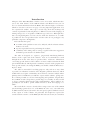
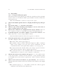
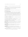
corpus ... pl. corpora ... 1. The body of a man or animal. (Cf. corpse.) Formerly
frequent; now only humorous or grotesque. 1854 Villikins & his Dinah (in Mus. Bouquet, No. 452), He
kissed her cold corpus a thousand times o’er. 2. Phys. A structure of a special character or function
in the animal body, as corpus callosum, the transverse commissure connecting the cerebral
hemispheres; so also corpora quadrigemina, striata, etc. of the brain, corpus spongiosum and
corpora cavernosa of the penis, etc.; corpus luteum L. luteus, –um yellow (pl. corpora lutea),
a yellowish body developed in the ovary from the ruptured Graafian follicle after discharge of
the ovum; it secretes progesterone and other hormones and after a few days degenerates unless
fertilization has occurred, when it remains throughout pregnancy. 1869 Huxley Phys. xi. 298 The
floor of the lateral ventricle is formed by a mass of nervous matter, called the corpus striatum. 1959 New
Biol. XXX. 79 As in mammals, glandular bodies known as corpora lutea are produced in the ovaries of
viviparous (and also of some oviparous) reptiles, in places from which the eggs have been shed at ovulation.
3. A body or complete collection of writings or the like; the whole body of literature on any
subject. 1727-51 Chambers Cycl. s.v., Corpus is also used in matters of learning, for several works of the
same nature, collected, and bound together.. We have also a corpus of the Greek poets.. The corpus of the
civil law is composed of the digest, code, and institutes. 1865 Mozley Mirac. i. 16 Bound up inseparably
with the whole corpus of Christian tradition. 4. The body of written or spoken material upon
which a linguistic analysis is based. 1956 W. S. Allen in Trans. Philol. Soc. 128 The analysis here
presented is based on the speech of a single informant.. and in particular upon a corpus of material, of
which a large proportion was narrative, derived from approximately 100 hours of listening. 1964 E. Palmer
tr. Martinet’s Elem. General Linguistics ii. 40 The theoretical objection one may make against the ‘corpus’
method is that two investigators operating on the same language but starting from different ‘corpuses’, may
arrive at different descriptions of the same language. 1983 G. Leech et al. in Trans. Philol. Soc. 25 We hope
that this will be judged.. as an attempt to explore the possibilities and problems of corpus-based research by
reference to first-hand experience, instead of by a general survey. 5. The body or material substance
of anything; principal, as opposed to interest or income. 1884 Law Rep. 25 Chanc. Div. 711 If these
costs were properly incurred they ought to be paid out of corpus and not out of income. phr. corpus
delicti (see quot. 1832); also, in lay use, the concrete evidence of a crime, esp. the body of a
murdered person. corpus juris: a body of law; esp. the body of Roman or civil law (corpus
juris civilis). 1891 Fortn. Rev. Sept. 338 The translation.. of the Corpus Juris into French. 1922 Joyce
Ulysses 451 (He extends his portfolio.) We have here damning evidence, the corpus delicti, my lord, a
specimen of my maturer work disfigured by the hallmark of the beast. 1964 Sunday Mail Mag. (Brisbane)
13 Sept. 3/3 An enthusiastic trooper, one of a party investigating river, dam and hollow log in search of the
corpus delicti, found some important evidence in a fallen tree. corpus vile Pl. corpora vilia Orig. in
phr. (see quot. 1822) meaning ‘let the experiment be done on a cheap (or worthless) body’. A
living or dead body that is of so little value that it can be used for experiment without regard
for the outcome; transf., experimental material of any kind, or something which has no value
except as the object of experimentation. 1822 De Quincey Confess. App. 189 Fiat experimentum
in corpore vili is a just rule where there is any reasonable presumption of benefit to arise on a large scale.]
1865 C. M. Yonge Clever Woman I. iii. 80 The only difficulty was to find poor people enough who would
submit to serve as the corpus vile for their charitable treatment. 1953 Essays in Criticism III. i. 4, I am
not proposing to include among these initial corpora vilia passages from either Mr Eliot’s criticism or Dr
Leavis’s.
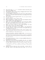
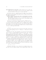
Definitions of corpus from OED 2
1 Corpus linguistics
1.1
What is a corpus?
We shall discuss what a corpus is by looking at how the word is used, in particular
by linguists. What kind of an object is a corpus, and what is it likely to be useful
for?
We learn the sense of a newly-encountered word in different ways. Young
children experimentally combine or mutate words to see which uses meet
with approval; older ones do the same in the process of defining peer groups
based on a shared exotic vocabulary. In both cases, meaning is exemplified
or confirmed by repeated, socially sanctioned, usage. One of the objectives of
traditional linguistics was to overcome this requirement of exposure to “language
in use” — an impractical option for those wishing to learn a new language
in a short time, or to understand a language no longer spoken anywhere —
by defining powerful general principles which would enable one to derive
the sense of any newly-encountered word simply by applying etymological or
morphological rules. Knowles (1996), arguing that linguistic theory is above all
a matter of organizing linguistic knowledge in this way, points for example to
the success with which such models have been used in training generations of
schoolchildren to understand Latin or Greek unseens.
While only experience can tell us what a word “is understood to mean”,
such analytic methods tell us what a word “ought to mean”. A modern
dictionary combines the strengths of both methods, by organizing evidence of
usage into an analytic framework of senses.
What, then, does the word ‘corpus’ actually mean? We might do worse
than consider the five distinct senses listed in the second edition of the Oxford
English Dictionary as a starting point (see figure on preceding page). Of these,
two particularly refer to language. The first is that of “A body or collection
of writings or the like; the whole body of literature on any subject”. Thus we
may speak of the ‘Shakespearean corpus’, meaning the entire collection of texts
by Shakespeare. The second is that of “the body of written or spoken material
upon which a linguistic analysis is based”. This is the sense of the word from
which the phrase ‘corpus linguistics’ derives, and in which we use it throughout
this book. The two senses can, of course, overlap — as when, for example, the
entire collection of a particular author’s work is subjected to linguistic analysis.
But a key distinction remains. In the words of John Sinclair, the linguist’s corpus
is “a collection of pieces of language, selected and ordered according to explicit
linguistic criteria in order to be used as a sample of the language” (Sinclair 1996).
It is an object designed for the purpose of linguistic analysis, rather than an object
defined by accidents of authorship or history.
1.  
5
As such, corpora can be contrasted with archives or collections whose components are unlikely to have been assembled with such goals in mind (see further
Atkins et al 1992). Given this emphasis on intended function, the composition
of a corpus will depend on the scope of the investigation. It may be chosen
to characterize a particular historical state or a particular variety of a particular
language, or it may be selected to enable comparison of a number of historical
states, varieties or languages. Varieties may be selected on geographical (for
example, British, American, or Indian English), sociological (for example, by
gender, social class, or age group), or generic bases (for example written vs.
spoken; legal or medical; technical or popular; private or public correspondence). Generally the texts to be included in a corpus are defined according
to criteria which are external to the texts themselves, relating to the situation of
their production or reception rather than any intrinsic property they may have.
Discovery of such intrinsic properties (if any) may, indeed, be the purpose of the
exercise.
Corpora stored and processed by computer, once the exception, are now
the norm. It is worth noting however that there is very little in the practice
of corpus linguistics which could not equally well be done in principle by nonautomatic means. However, in general, corpora are understood to be computerprocessable corpora.
The British National Corpus (BNC) consists of a sample collection which
aims to represent the universe of contemporary British English. Insofar as it
attempts to capture the full range of varieties of language use, it is a balanced
corpus rather than a register-specific or dialect-specific one; it is also a mixed corpus,
containing both written texts and spoken ones — transcriptions of naturallyoccurring speech.
1.2 What can you get out of a corpus?
A corpus can enable grammarians, lexicographers, and other interested parties
to provide better descriptions of a language by embodying a view of it which
is beyond any one individual’s experience. The authoritative Comprehensive
Grammar of the English Language (Quirk et al 1985) was derived in part from
evidence provided by one of the first modern English corpora, the Survey
of English Usage. Svartvik and Quirk (1980: 9) observe that: “Since native
speakers include lawyers, journalists, gynaecologists, school teachers, engineers,
and a host of other specialists, it follows: (a) that no individual can be expected to
have an adequate command of the whole ‘repertoire’: who, for example, could
equally well draft a legal statute and broadcast a commentary on a football game?
(b) that no grammarian can describe adequately the grammatical and stylistic
6
:     
properties of the whole repertoire from his own unsupplemented resources:
‘introspection’ as the sole guiding star is clearly ruled out.”
A corpus which is designed to sample the entire ‘repertoire’ offers a tool
for the description of properties with which even the grammarian may not be
personally familiar. Corpus-based descriptions have produced a few surprises,
sometimes contradicting the received wisdom. Sampson (1996) describes how
he became a corpus linguist as a result of his experience with theories of
recursive ‘central embedding’ in sentences such as ‘the mouse the cat the dog
chased caught squeaked’, where component clauses nest within each other like
Russian dolls. Most discussions of this phenomenon had used linguistic intuition
to analyze entirely imaginary sentences, claiming that such constructions were in
some sense ‘unnatural’, though syntactically feasible. However, when Sampson
turned to look at corpus data, he found that such centrally embedded structures
were actually far from rare, and used in ways which appeared entirely ‘natural’.
While it does not eliminate linguistic intuition in classifying and evaluating
instances, the use of corpora can remove much of the need to invent imaginary
data, and can provide relatively objective evidence of frequency.
The utility of a corpus to the lexicographer is even more striking: careful
study of a very large quantity and wide range of texts is required to capture and
exemplify anything like all the half-million or more words used in contemporary
British English. It is no coincidence that dictionary publishers have played
major roles in setting up the two largest current corpora of British English:
the Bank of English (HarperCollins) and the BNC (Oxford University Press,
Longman, Chambers); or that, in the increasingly competitive market for
English language learners’ dictionaries, four new editions published in 1995
(the Collins Cobuild Dictionary, the Cambridge Dictionary of International English,
the Longman Dictionary of Contemporary English, the Oxford Advanced Learner’s
Dictionary) should all have made the fact of their being ‘corpus-based’ a selling
point.
Linguists have always made use of collections of textual data to produce
grammars and dictionaries, but these have traditionally been analyzed in a
relatively ad hoc manner, on the basis of individual salience, with a consequent
tendency to privilege rare and striking phenomena at the expense of mundane
or very high frequency items. Corpora, in particular computer-processable corpora, have instead allowed linguists to adopt a principle of ‘total accountability’,
retrieving all the occurrences of a particular word or structure in the corpus
for inspection, or (where this would be infeasible) randomly selected samples.
This generally involves the use of specialized software to search for occurrences
(or co-occurrences) of specified strings or patterns within the corpus. Other
1.  
7
software may be used to calculate frequencies, or statistics derived from them, for
example to produce word lists ordered by frequency of occurrence or to identify
co-occurrences which are significantly more (or less) frequent than chance.
Concordances are listings of the occurrences of a particular feature or combination of features in a corpus. Each occurrence found, or hit, is displayed with
a certain amount of context — the text immediately preceding and following
it. The most commonly used concordance type (known as KWIC for ‘Key
Word In Context’) shows one hit per line of the screen or printout, with the
principal search feature, or focus, highlighted in the centre. Concordances also
generally give a reference for each hit, showing which source text in the corpus
it is taken from and the line or sentence number. It is then up to the user to
inspect and interpret the output. The amount of text visible in a KWIC display
is generally enough to make some sense of the hit, though for some purposes,
such as the interpretation of pronominal reference, a larger context may have to
be specified. Most concordancing software allows hits to be formatted, sorted,
edited, saved and printed in a variety of manners.
Frequency counts are implicit in concordancing, since finding all the occurrences of a particular feature in the corpus makes counting the hits a trivial
task. Software will generally allow numbers to be calculated without actually
displaying the relevant concordance — an important feature where thousands or
even millions of occurrences are involved. Frequency counts can be elaborated
statistically, in many cases automatically by the concordancing software, but
should be interpreted with care (see further 2.2.4 on page 40).
Concordances and frequency counts can provide a wide variety of linguistic
information. We list some of the kinds of questions which may be asked, relating
to lexis, morphosyntax, and semantics or pragmatics.
A corpus can be analyzed to provide the following kinds of lexical information:
How often does a particular word-form, or group of forms (such as the
various forms of the verb ‘start’: ‘start’, ‘starts’, ‘starting’, ‘started’) appear
in the corpus? Is ‘start’ more or less common than ‘begin’? The relative
frequency of any word-form can be expressed as a z-score, that is, as the
number of standard deviations from the mean frequency of word-forms
in the corpus. The number of occurrences of a word-form in the entire
BNC ranges from over 6 million for the most frequent word, ‘the’, to
1 for ‘aaarrrrrrrrggggggghhhhhh’ or ‘about-to-be-murdered’. The mean
frequency is approximately 150, but the standard deviation of the mean is
very high (over 11,000), indicating that there are very many words with
frequencies far removed from the mean.
8
:     
With what meanings is a particular word-form, or group of forms, used?
Is ‘back’ more frequently used with reference to a part of the body or a
direction? Do we ‘start’ and ‘begin’ the same sorts of things?
How often does a particular word-form, or group of forms, appear near
to other particular word forms, which collocate with it within a given
distance? Does ‘immemorial’ always have ‘time’ as a collocate? Is it more
common for ‘prices’ to ‘rise’ or to ‘increase’? Do different senses of the
same word have different collocates?
How often does a particular word-form, or group of forms, appear in
particular grammatical structures, which colligate with it? Is it more
common to ‘start to do something’, or to ‘start doing it’? Do different
senses of the same word have different colligates?
How often does a particular word-form, or group of forms, appear in
a certain semantic environment, showing a tendency to have positive or
negative connotations? Does the intensifier ‘totally’ always modify verbs
and adjectives with a negative meaning, such as ‘fail’ and ‘ridiculous’?
How often does a particular word-form, or group of forms, appear in
a particular type of text, or in a particular type of speaker or author’s
language? Is ‘little’ or ‘small’ more common in conversation? Do women
say ‘sort of ’ more than men? Does the word ‘wicked’ always have positive
connotations for the young? Is the word ‘predecease’ found outside legal
texts and obituaries? Do lower-class speakers use more (or different)
expletives?
Whereabouts in texts does a particular word form, or group of forms,
tend to occur? Does its meaning vary according to its position? How
often does it occur within notes or headings, following a pause, near the
end of a text, or at the beginning of a sentence, paragraph or utterance?
And is it in fact true that ‘and’ never begins a sentence?
A corpus can also be analyzed to provide the following kinds of morphosyntactic information:
How frequent is a particular morphological form or grammatical structure? How much more common are clauses with active than with passive
main verbs? What proportion of passive forms have the agent specified in
a following ‘by’ phrase?
With what meanings is a particular structure used? Is there a difference
between ‘I hope that’ and ‘I hope to’?
How often does a particular structure occur with particular collocates or
colligates? Is ‘if I was you’ or ‘if I were you’ more common?
1.  
9
How often does a particular structure appear in a particular type of text,
or in a particular type of speaker or author’s language? Are passives
more common in scientific texts? Is the subjunctive used less by younger
speakers?
Whereabouts in texts does a particular structure tend to occur? Do writers
and speakers tend to switch from the past tense to the ‘historic present’ at
particular points in narratives?
And, finally, a corpus can be analyzed to provide semantic or pragmatic
information. Rather than examining the meanings and uses of particular forms,
we can use it to identify the forms associated with particular meanings and uses:
What tools are most frequently referred to in texts talking about gardening?
What fields of metaphor are employed in economic discourse?
Do the upper-middle classes talk differently about universities from the
working classes?
How do speakers close conversations, or open lectures? How do chairpersons switch from one point to another in meetings?
Are pauses in conversation more common between utterances than within
them?
What happens when conversationalists stop laughing?
Not all of these types of information are equally easy to obtain. In using
concordancing software, specific strings of characters have to be searched for.
In order to disambiguate homographs or to identify particular uses of words or
structures, it may be necessary to inspect the lines in the output, classifying them
individually. Thus while it is relatively easy to calculate the frequency of a wordform and of its collocates, it may be more difficult to calculate its frequency
of use as a particular part of speech, with a particular sense, or in a particular
position or particular kind of text.
To help in such tasks, computer corpora are increasingly marked up with
a detailed encoding which encompasses both external characteristics of each
text and its production, and internal characteristics such as its formal structure.
Such information will typically include details of what kind of text it is and
where it comes from, details relating to the structure of the text and the status of
particular components — division into chapters, paragraphs, spoken utterances,
headings, notes, references, editorial comments etc., as well as any linguistic
annotation, indicating for instance the part-of-speech value or the root form of
each word. Such encoding permits the user to search for strings or patterns in
:     
10
particular kinds, parts or positions of texts, or with particular types of linguistic
annotation.
It can be equally difficult to find instances of particular syntactic, semantic
or pragmatic categories unless these happen to have clear lexical correlates, or
the corpus markup clearly distinguishes them. For instance, the markup of the
BNC might be used to find occurrences of highlighting (typically through italics
or underlining in the original), to investigate headings and captions, to generate
a list of the publishers responsible for the texts in the corpus, or to identify those
texts published by specific publishers.
While the examples just cited have all concerned analyses within a particular
corpus, it is evident that all these areas can also be examined contrastively,
comparing data from corpora of different languages, historical periods, dialects
or geographical varieties, modes (spoken or written), or registers. By comparing
one of the standard corpora collected twenty years ago with an analogous corpus
of today, it is possible to investigate recent changes in English. By comparing
corpora collected in different parts of the world, it is possible to investigate
differences between, for instance, British and Australian English. By comparing
a corpus of translated texts with one of texts originally created in the target
language, it is possible to identify linguistic properties peculiar to translation.
By comparing a small homogeneous corpus of some particular kind of material
with a large balanced corpus (such as the BNC), it is possible to identify the
distinctive linguistic characteristics of the former.
1.3
How have corpora been used?
This section describes a few major corpora which have previously been created
and discusses some of the work done with them, to illustrate current concerns
in the field.
1.3.1 What kinds of corpora exist?
We begin by listing some of the main corpora developed for English in the past,
grouped according to the main areas of language use they sample. For a fuller
annotated list, see Edwards (1993) or Wichmann et al (in press).
geographical varieties The earliest corpus in electronic form, compiled at
Brown University in 1964, contained 1 million words of written American English published in 1961 (Kucera and Francis 1967). The Brown
corpus has since been widely imitated, with similarly-designed corpora
being compiled for British (the Lancaster-Oslo-Bergen corpus or LOB:
Johansson 1980), Indian (the Kolhapur Corpus of Indian English: Shastri
1988), Australian (the Macquarie Corpus of Australian English: Collins
and Peters 1988) and New Zealand varieties (the Wellington corpus:
1.  
11
Bauer 1993). The International Corpus of English project (ICE) is
currently creating a corpus with similarly-designed components representing each of the major international varieties of contemporary English
(Greenbaum 1992).
spoken language corpora The earliest computer corpora, such as Brown and
LOB, were collections of written data. A number of corpora consisting
of transcripts of spoken English have since been developed. These vary
enormously both in the types of speech they include and in the form and
detail of transcription employed (see 1.4.2 on page 26). The best-known is
probably the London-Lund Corpus, a computerised version of just under
half-a-million words of the Survey of English Usage conversational data
(Svartvik 1990; Svartvik and Quirk 1980), which has been widely used
in comparisons with the LOB corpus of written English. The Corpus of
Spoken American English under development at Santa Barbara (Chafe et
al 1991) is collecting a similar quantity of American conversational data.
mixed corpora The major large mixed corpus to precede the BNC was the
Birmingham collection of English texts, developed at the University of
Birmingham with the dictionary publishers Collins during the 1980s as
a basis for the production of dictionaries and grammars (see e.g. Sinclair
1987). This originally contained 7.5 million words, growing eventually
to nearly 20 million, of which approximately 1.3 million were transcripts
of speech. The collection has continued to grow since, having now been
incorporated into the 300 million word Bank of English (see 1.4.1 on
page 21).
historical varieties The most extensive corpus of historical English is probably
the Helsinki corpus of English texts: diachronic and dialectal (Kytö 1993).
The corpus has three parts, corresponding with three historical periods
(Old, Middle, and Early Modern English); within each period, there are
samples of different dialects, permitting not only diachronic comparisons
but also synchronic comparisons of different geographical varieties.
child and learner varieties A number of corpora have been compiled relating to particular categories of language users, in particular children
who are acquiring English as their first language, and foreign learners of
English. They are sometimes termed special corpora (Sinclair 1996), because
they document uses of language which are seen as deviant with respect to
a general norm. Instances include the Polytechnic of Wales corpus of child
language (O’Donoghue 1991), and the International Corpus of Learner
English (ICLE) being created at Louvain (Granger 1993).
12
:     
genre- and topic-specific corpora Other corpora have been designed to
include only samples of language of a particular type, for example dealing
with a particular topic, or belonging to a particular genre or register.
There are many examples, ranging from psycholinguistically motivated
experiments such as the HCRC map task corpus (Anderson et al 1991),
consisting of 128 transcribed performances of map-reading tasks, to
corpora created for other purposes, such as the Hong Kong corpus
of computer science texts, designed to support analysis of technical
vocabulary (Davison 1992). In the USA, the Linguistic Data Consortium
has produced a large number of corpora of specific genres of speech and
writing on CD-ROM, ranging from telephone conversations to stockexchange reports.
multilingual corpora Monolingual corpora of languages other than English
are not mentioned here for reasons of space, but a number of multilingual
corpora containing texts in both English and one or more other languages
have been developed. Some are fairly heterogeneous collections, while
others are carefully constructed ensembles of texts selected on the basis of
similar criteria in each language. In the former category, the European
Corpus Initiative (ECI) has produced a multilingual corpus of over 98
million words, covering most of the major European languages, as well
as Turkish, Japanese, Russian, Chinese, Malay and more (ArmstrongWarwick et al 1994). In the latter category, an EU-funded project called
PAROLE is currently building directly comparable corpora for each major
European language.
1.3.2 Some application areas
The range of corpus-based descriptive work is well documented by Altenberg’s
bibliographies of corpus linguistics (Altenberg 1990, 1995), and is also covered
in a number of introductory textbooks on the field. Recent examples include
Sinclair (1991), Stubbs (1996) and McEnery and Wilson (1996); Leech and
Fligelstone (1992) and Biber et al (1996) provide accessible short introductions.
In this section, we review a handful of studies in order to illustrate some of the
areas in which corpus-based work has been carried out, and to raise some of the
key methodological issues. No claim to completeness of coverage is intended, as
the field is both very varied and rapidly expanding. For up-to-date information,
and for a wider (more corpus-like!) perspective, the reader could do a lot worse
than to search the World Wide Web for pages on which the phrase ‘corpus
linguistics’ appears.
Corpus-based research naturally grounds its theorizing in empirical observation rather than in appeals to linguistic intuition or expert knowledge. It thus
1.  
13
emphatically rejects one of the major tenets of Chomskian linguistics, namely
that the linguist’s introspection provides the only appropriate basis for describing
language, insofar as “information about the speaker-hearer’s competence . . . is
neither presented for direct observation nor extractable from data by inductive
procedures of any known sort” (Chomsky 1965: 18). Corpus users have taken
varying positions on these issues, ranging from the ‘weak’ view, that sees corpus
data as complementing the ‘armchair’ linguist’s intuitive insights by providing
real-life examples and a reliable testbed for hypotheses (see 8.1 on page 143),
to the ‘strong’ view, according to which corpus data should always override
intuition, and discussion should be confined solely to naturally-occurring examples. In either case, corpus-based work has wider affinities than many other
branches of linguistics, since the study of language-in-use has something to offer
historical, political, literary, sociological, or cultural studies, and has profited
from the resulting synergy.
Our discussion focuses on four application areas: the emergence of collocation
as a key component in linguistic description; the opportunities afforded by
corpus-based methods for contrastive studies of different languages, varieties and
registers; the use of corpora in natural language processing (NLP); and finally, their
use in foreign language teaching.
1.3.3 Collocation
One of the forefathers of contemporary corpus linguistics, J.R. Firth, observed
that part of the meaning of the word ‘ass’ consists in its habitual collocation
with an immediately preceding ‘you silly’ (Firth 1957: 11). (Whether this use is
still current some fifty years later is a question the BNC can answer: there are
in fact only 8 occurrences of ‘silly ass’ in the corpus, none of them preceded
by ‘you’.) There are a great many cases in English where the occurrence of
one word predicts the occurrence of another, either following or preceding
it. Kjellmer (1991) notes such examples as ‘billy’, which predicts ‘goat’ or
‘can’ following, and ‘bail’, which predicts ‘jump’ or ‘stand’ preceding. Such
collocational patterns tend to be highlighted by KWIC concordances, since
these show just the few words which precede and follow the keyword or focus,
and can typically be sorted according to these words. It is also relatively easy
to calculate the frequency with which a particular collocate appears within a
certain range of the focus — its collocation frequency within a given span — and to
compare such frequencies to find the most common collocates occurring, say,
up to two words before ‘ass’.
Jones and Sinclair (1974) claim that the probabilities of lexical items occurring in English are generally affected by collocational norms within a span
of up to four words. Co-occurrence of two or more words within a short
14
:     
space can be important insofar as that co-occurrence is expected and typical
(whether in the language in general, in a particular text-type, or in the style
of a particular speaker or author), or insofar as it is unexpected and atypical.
Sinclair (1991) argues that recurrent collocational patterns effectively distinguish
different senses of the same word — a ‘silly ass’, while potentially a quadruped,
is statistically a biped — and that consequently collocational frequencies can be
used to disambiguate word senses. In this he builds on Firth’s view that for
the lexicographer, “each set of grouped collocations may suggest an arbitrary
definition of the word, compound or phrase which is being studied” (Firth
1957: 196). From a converse perspective, deviation from a collocational norm
— ‘since breakfasts immemorial’, say — can be a means of generating particular
effects, such as irony (Louw 1993).
The tendency for one word to occur with another has both grammatical and
semantic implications. The collocation of a word with a particular grammatical
class of words has been termed colligation. For instance, unlike ‘look at’, the
verb ‘regard’ appears always to colligate with adverbs of manner, as in ‘She
regarded him suspiciously’ (Bolinger 1976). From a semantic perspective, the
habitual collocations of some words mean that they they tend to assume the
positive or negative connotations of their typical environments — a particular
semantic prosody. For example, Sinclair (1991) notes that the verb ‘set in’ has a
negative prosody, because things which typically set in are ‘rot’, ‘decline’ etc.,
making it extremely difficult to use this verb with positive implications. In
the same way, the typical collocations of many apparently neutral terms may
reveal deep-seated cultural prejudices: Stubbs (1996: 186ff.) notes how the
high-frequency collocates of terms such as ‘Welsh’ or ‘Irish’ tend to reinforce
nationalistic stereotypes.
Other than in set phrases, collocations and their frequencies are not generally
accessible to intuition. They can however be easily identified and quantified by
computational methods, in corpora which are sufficiently large for the purpose.
Work based on the Birmingham collection of English texts, revealing the
extent of collocational patterning in English, has contributed to change current
views of psycholinguistic organization, by providing important evidence that
lexical items are to a large extent co-selected rather than combined individually,
following what Sinclair terms an idiom principle rather than an open-choice one.
A collection of concordances showing the most frequent collocates of some
10,000 words in the Bank of English has recently been published on CDROM (Cobuild 1995). Much discussion and research has also been dedicated
to the development of appropriate measures of the strength of collocational
1.  
15
links (Dunning 1993; Stubbs 1995), and to the automatic listing of significant
collocations.
1.3.4 Contrastive studies
The construction of the LOB corpus of British English, on closely parallel lines
to the Brown corpus of American English, and their subsequent morphosyntactic annotation (see 1.4.2 on page 24), stimulated a variety of comparative studies,
facilitated by the wide distribution of both corpora on a single CD-ROM by
ICAME, a highly influential organization of European corpus linguists based at
the University of Bergen in Norway. This section reviews some examples of
contrastive studies, involving both different corpora and different components
of a single corpus, with the purpose of illustrating some of the methodological
issues involved.
Comparing geographical varieties and languages Hofland and Johansson (1982) and Johansson and Hofland (1989) report detailed studies of word
frequencies in the Brown and LOB corpora, showing, for instance, that 49 of
the 50 most frequent words in each corpus are the same. Contrasts concern
not only such areas as spelling (e.g. ‘colour’ vs. ‘color’), and different choices
of synonyms (e.g. ‘transport’ vs. ‘transportation’, ‘film’ vs. ‘movie’), but
also different subject matter (e.g. ‘tea’ vs. ‘coffee’, ‘London’ vs. ‘Chicago’).
Leech and Falton (1992) suggest that some of these differences in frequency may
indicate cultural, rather than simply linguistic differences. Noting, for instance,
the considerably more frequent use in Brown of military terms, such as ‘armed’,
‘army’, ‘enemy’, ‘forces’, ‘missile(s)’, ‘warfare’, they suggest that this may reflect
a greater concern in the US with military matters (remembering that 1961, the
year of the Brown texts, was also that of the Cuban missile crisis). And faced
with the greater frequency in LOB of conditional and concessive conjunctions
(‘if ’, ‘but’, ‘although’, ‘though’) and words denoting possibility or uncertainty
(‘possible’, ‘perhaps’, ‘unlikely’ etc.), they speculate that this may conform to
the stereotype of the “wishy-washy Briton who lacks firmness and decisiveness”
(Leech and Falton 1992: 44).
In reaching these (tentative) conclusions, they note that a relatively small
number of words can be analyzed in this way. The LOB and Brown corpora
each contain only 50,000 word types (less than the number of headwords in a
single-volume dictionary), and among the less frequent words, relative frequency
or infrequency may be due to sampling bias. Even at higher frequency levels,
differences may be the product of a skewed distribution across texts. While the
influence of these sources of error can be reduced by comparing groups of words
identified by semantic or other criteria, careful examination of concordances
remains necessary to check how often the word or words in question are in fact
16
:     
used with a particular sense — not all occurrences of the word ‘film’ refer to
cinema, and ‘tea’ is a meal in some parts of Britain, as well as a drink.
Multilingual, comparable and parallel corpora There is an increasing
tendency to apply corpus techniques to the task of comparing different languages. Where a corpus consists of texts selected using similar criteria in two
or more languages, comparisons can be made at many different levels, ranging
from lexicogrammatical preferences to rhetorical organization. One particularly
interesting type of multilingual corpus is the parallel corpus, consisting of texts that
are actually translations of each other: prototypical instances are official documents produced in multilingual environments, such as the UN and EU, or the
Canadian Hansard, which is published in both English and French. Such corpora
have clear utility for the study of translation itself, as well as providing a useful
focus for contrastive studies of the differences between particular languages.
To facilitate comparison, the texts in parallel corpora may be aligned,
identifying equivalences on a sentence-by-sentence, phrase-by-phrase, or wordby-word basis, and much effort has gone into the development of software to
align parallel texts automatically. The major fields of application have so far
been in developing and testing machine translation packages and producing
computerized translation aids (such as bilingual dictionaries and terminology
databanks), but such corpora also have much to teach about the universals and
specifics of language, and the process of translation. For instance, the EnglishNorwegian parallel corpus project (Johansson and Hofland 1993; Johansson
and Ebeling 1996; Aijmer et al 1996) lists among its fields of investigation not
only the similarities and differences in the lexicogrammatical, rhetorical, and
information structure of texts in the two languages, but also such questions as:
To what extent are there parallel differences in text genres across languages?
In what respects do translated texts differ from comparable original texts
in the same language?
Are there any features in common among translated texts in different
languages (and, if so, what are they)?
Comparing diachronic varieties English-language corpus-building dates
back at least thirty years. The continued availability of these pioneering corpora
has made possible a range of contrastive studies investigating changes in the
English language over time. There is also a growing interest in the construction
of specifically designed diachronic corpora which sample language production over
much longer time periods.
1.  
17
Examples of the first kind include a 1991 version of LOB, using identical
sampling criteria as far as possible, recently completed at Freiburg (Mair 1993).
As well as facilitating diachronic comparison of particular linguistic features, such
corpora may also provide a useful yardstick for comparing studies based on the
larger corpora of recent years with ones based on the smaller corpora which
preceded them.
Notable examples of the second kind include the Archer corpus (Biber,
Finegan and Atkinson 1994), which contains samples of eleven different registers
from different historical periods, and the Helsinki corpus of English texts:
diachronic and dialectal (Kytö 1993: see 1.3.1 on page 10). Kytö et al (1995)
provides a useful checklist of new projects in this expanding field.
Change over time can also be investigated by contrasting the usage of
different age groups, as further discussed in the next section.
Comparing categories of users Where corpora provide information as
to the social and linguistic provenance of speakers and hearers, or of writers
and readers, they can be used to compare the language of different groups
according to such variables as region, age, sex, and social class, provided that a
demographically balanced sample of language users has been taken. For instance,
Stenström (1991) used the London-Lund corpus to study the relationship
between gender and the use of expletives relating to religion, sex and the body
in speech. She found that while female speakers tended to use such words more
often than male, they tended to choose expletives from a ‘heaven’ group, while
male speakers used ones relating to ‘hell’ and ‘sex’. Investigating the function of
these words in the light of their position in the utterance, she also found that the
male speakers used them to emphasize their own contributions, whereas female
speakers used them to give responses and invitations to continue.
Comparing different uses of language The construction of the LondonLund corpus of spoken English spawned a large number of studies comparing
speech with writing, generally using the LOB corpus as evidence of the latter.
These have highlighted differences in the relative frequencies of words and
structures in the two modes (in speech the most common word is ‘I’, while
in writing it is ‘the’), as well as facilitating the identification and description of
features whose use appears to be specific to the spoken language, most notably
discourse-structuring elements such as ‘well’, ‘I mean’, and ‘you know’.
Corpora have also been extensively used to investigate the ways in which
genres differ linguistically, attempting to characterize genres by the relative
frequency of particular features. Conversely, insofar as texts can be categorized
statistically according to linguistic features, what correspondence is there between those categorizations and the lists of text-types employed, for instance, in
18
:     
corpus design? Biber (1988) compared the frequencies of a range of linguistic
features which can be automatically counted (word length, type/token ratio,
nouns, prepositions, first/second/third person pronouns, tense, voice, aspect,
‘wh-’ relative clauses, synthetic vs. analytic negation, ‘private’ vs. ‘public’ verbs,
etc.) in samples from texts of different types in the LOB and London-Lund
corpora, using cluster and factor analysis to identify eight basic classes of text,
grouped by similar scores on five dimensions of variation. Biber and Finegan
(1994) employ similar methods to investigate variation within texts, showing
that in medical research articles, frequencies of a number of lexicogrammatical
phenomena vary according to the section of the article sampled.
1.3.5 NLP applications
There has recently been an increased awareness of the potential which corpus
methods offer for tackling a number of problems in the field of natural language
processing (NLP), that is, the development of automatic or semi-automatic
systems for analyzing, ‘understanding’, and producing natural language.
Corpora are increasingly used in the development of NLP tools for applications such as spell-checking and grammar-checking, speech recognition,
text-to-speech and speech-to-text synthesis, automatic abstraction and indexing,
information retrieval, and machine translation. A major problem to be faced by
all NLP systems is that of resolving ambiguity, be this selecting which of two
or more possible orthographic transcriptions might match a given acoustic input
(‘whales’, ‘Wales’, or ‘wails’?), or deciding whether an instance of the word
‘bank’ refers to a financial institution or a landscape feature, and hence how it
should be translated into, say, French, or how the text that contains it should be
classified for retrieval purposes.
The limited results achieved in such areas using traditional rule-based models
of language have led to an increasing interest in probabilistic models, where
probabilities are calculated on the basis of frequencies in corpus data (Church
and Mercer 1993). Traditional spell-checkers, for instance, are based only on
a dictionary of possible orthographic forms in the language, so that they fail
to recognize errors which are nonetheless acceptable forms (such as ‘form’
for ‘from’). Performance in such cases can be improved by considering the
probability that the form typed by the user will occur after the previous word,
where this probability has been calculated by analyzing a corpus for the language
concerned. (For instance, it is highly unlikely that the word between ‘the’ and
‘typed’ in the previous sentence could be ‘from’.)
The analysis of frequencies of particular features in corpora underlies a wide
variety of NLP applications based on probabilistic techniques, such as:
1.  
19
categorization of specific texts, for instance by identifying their type,
semantic field, and keywords as a basis for automatic indexing and
abstracting, or extracting terminology;
refinement of question-answering and information retrieval systems, enabling them to employ or suggest additional or alternative search terms
to interrogate textual databases, on the basis of collocational regularities in
corpus data, and to filter retrieved information by checking its conformity
to the typical collocational patterns of the search terms proposed;
improvement of multilingual retrieval of texts, and identification of terminological equivalents in different languages, on the basis of lexical
and collocational equivalences identified in parallel multilingual corpora
(see 1.3.4 on page 15).
A further use of corpora in NLP is as testbeds to evaluate applications, be
these theoretically motivated or probabilistic. Probabilistic models of language
can, to a certain extent, be self-organizing, and in this respect corpora can
provide training instruments for software which learns probability through
experience, or refines an initial model in a bootstrapping process (Atwell 1996).
A system which needs to disambiguate the term ‘bank’, for instance, can analyze
a corpus to learn that the landscape sense generally collocates with ‘river’,
‘flower’, etc., while the financial one collocates with ‘merchant’ and ‘high street’.
Such uses typically call for substantial annotation of corpora in order to reduce
ambiguity in the training materials, and NLP applications in many cases overlap
with applications designed to annotate corpora in various ways (see 1.4.2 on
page 24).
1.3.6 Language teaching
The growing variety of corpus applications in the field of English language
teaching is reviewed by Murison-Bowie (1996). Corpora have already had a
considerable influence in the creation of new dictionaries and grammars for
learners, where the use of corpus data has allowed:
more accurate selection of words and senses for inclusion, based on
frequency of occurrence;
introduction of information concerning the relative frequency of each
word and of the different senses of each, and their use in different genres
and registers;
citation of actual rather than invented examples, selected to illustrate
typical uses and collocations.
Sinclair (1987) provides a detailed discussion of these issues in reference to
the creation of the Collins Cobuild Dictionary.
20
:     
Kennedy (1992) reviews the long tradition of pre-electronic corpus work
in language teaching. Many of the studies he discusses aimed to identify the
most frequent words and grammatical structures in the language, with a view
to optimizing the design of syllabuses and the grading of materials. Such goals
have received new impetus from the availability of electronic corpora. Analysis
of the Birmingham collection of English texts underlay the selection of the
‘lexical syllabus’ proposed by Willis (1990); Grabowski and Mindt (1995) used
the Brown and LOB corpora to create a list of irregular verbs ordered according
to frequency, arguing that by following this order in syllabus design, teaching
should achieve maximum yield for the student’s effort, irrespective of when the
learning process is broken off.
Corpus data have also provided a means of evaluating conventional syllabuses. Ljung (1991) compares the lexis of textbooks of English as a foreign
language with that of a corpus of non-technical writing, while Mindt (1996)
compares the treatment of future time reference in textbooks and learner
reference grammars with corpus data. Such studies use corpora to highlight
actual frequency of occurrence, which, while not the only criterion for deciding
syllabus content or the form of materials (Widdowson 1991), can clearly provide
teachers and textbook writers with an important tool to assess the pedagogic
suitability and adequacy of particular choices (Biber et al 1994).
There is also a growing interest in providing teachers and learners with direct
access to corpora as resources for classroom or individual work. Fligelstone
(1993) suggests that learners can use corpora to find out about the language
for themselves and hence to question prescriptive specifications, for instance
by exploring the nature of idioms and collocations, rhetorical questions, the
use of sentence-initial ‘and’, etc. Similarly, Aston (in press) argues that with
appropriate training, advanced learners can use large corpora as reference tools
which overcome many of the limitations of existing dictionaries and grammars
by providing a much larger number of more contextualized examples. Corpora
may not only be a source of information about the language in question:
Fligelstone notes that they can also provide encyclopedic knowledge, making
them a useful tool to gather ideas about a subject in order to write or talk about
it, while Aston (1995) suggests that concordancing software enables learners
to browse the corpus texts in a serendipitous process where they not only
analyze language but experience it as communicative use. In such ways the
growing availability of corpora offers learners a new kind of resource which can
complement the traditional dependency on teacher, textbook, and reference
book.
1.  
21
1.4 How should a corpus be constructed?
We noted above that a corpus is not a random collection of text. In this
section, we review some of the major issues relating to corpus construction.
We discuss first some basic design principles, concerning size, sampling practice,
and composition, and then consider the various kinds of encoding, annotation,
and transcription policies which may be adopted.
1.4.1 Corpus design
In designing a corpus to address a particular purpose, two groups of criteria must
be considered. On the one hand the size of the corpus and of its component
parts, and on the other the material actually selected for inclusion, may each
have crucial effects on its usability.
Corpus size and sample size The frequency of different word forms in a
corpus generally follows a Zipfian distribution (Zipf 1935), whereby the second
most frequent word occurs approximately half as often as the most frequent one,
the third most frequent word approximately one third as often, and so on. All
but the most frequent words are extremely rare. Corpora therefore need to be
very large and heterogeneous if they are to document as wide as possible a range
of uses of as many linguistic features as possible.
Even where they are relatively frequent, features which are unevenly distributed across different types of text in the corpus may not be adequately
represented. Sinclair (1991: 24) notes of the Brown and LOB corpora that
they only provide reliable sources of information concerning relatively frequent
words that occur in a wide range of texts. They are much less reliable for words
which occur only in certain text-types, because “the sub-categories necessary
to balance the sample are not in themselves reasonable samples because they are
too brief ”. Increasing corpus size can go some way to solving these problems
by providing larger samples for each sub-category.
While an increase in size provides more data, it also tends to entail less
detailed analyses: it is striking how many descriptive studies have analyzed only
small corpora (or small samples of larger ones), often because of the need to
inspect and categorize data manually. The analysis of larger corpora is heavily
dependent on the use of automatic or semi-automatic procedures able to identify
particular linguistic phenomena (see 1.4.2 on page 24). The availability of such
procedures is still limited in many areas.
Sinclair (1991: 24ff.) has argued that the static sample corpus consisting of
a fixed collection of data should ideally give way to the monitor corpus where
information could be gleaned from a continuous stream of new text “as it
passes through a set of filters which will be designed to reflect the concerns
of researchers.” In the lexicographical field, for instance, procedures might be
22
:     
designed to capture new word forms or usages, and shifts in frequency of use.
Such a corpus would allow the user to detect phenomena which would be
inadequately represented in even a very large sample corpus, and to monitor
changes in the language as they took place. The Bank of English project at the
University of Birmingham puts this idea into practice (Sinclair 1992). At the
time of writing, this corpus contains over 300 million words, but is continually
expanding and being monitored by a set of software tools which categorize
incoming data automatically for particular purposes.
In order to include both a wide range of text-types and a large number
of different texts of each type, early corpora included relatively brief extracts
from each text sampled: the one million-word Brown and LOB corpora
each consisted of randomly-selected 2000-word samples from 500 texts, of 15
different types. A corpus composed of short samples of equal length is less likely
to give skewed results due to the influence of particular source texts, but is of
little use for the study of large textual features such as narrative organization, or
of within-text variation (Biber and Finegan 1994). To permit the study of such
phenomena, Sinclair (1996) has argued that large corpora should be composed
of whole texts wherever possible.
The continued growth in the size of corpora has generally implied an
increase in sample sizes as well as in the number of samples. However, the
inclusion of complete texts may not always be possible, either for copyright
reasons, or because the notion of ‘completeness’ is inappropriate or problematic
(Is a newspaper a complete text? Is each story in a newspaper a complete text?).
Complete texts may also vary greatly in size, giving rise to problems of balance.
Corpus composition A corpus which claims to ‘characterize the state of a
language’ must define both the linguistic universe which has been sampled and
the sampling procedures followed. Is it intended to characterize only the speech
and writing of competent native-speakers? If so, how are the latter to be defined?
Is it to include as wide a variety of different types of language as possible? Should
its composition reflect the relative frequencies with which these different types
occur? And if so, should these frequencies be calculated on the basis of reception
(the language people hear and read), production (the language people speak and
write), or both? In the first case priority will be given to those text-types
which are most widely and frequently experienced, such as casual conversation,
everyday workplace and service encounters, television, radio and the popular
press. In the second case, while much of the everyday dialogue content may
be similar, the rest of the corpus may look very different, since most texts are
produced for small audiences.
1.  
23
Many of the criteria for the composition of a corpus are determined by its
intended uses. The Survey of English Usage aimed to describe the grammatical
repertoire of adult educated speakers of English with the aid of a corpus which
was “reasonably representative of the repertoire of educated professional men
and women in their activities, public and private, at work and at leisure, writing
and speaking” (Quirk 1974: 167). Given these goals, it was designed to sample
a wide range of text types, deciding the proportions of each largely on their
assumed frequency of production in the language as a whole. Most large mixed
corpora have tended to follow the Survey in aiming to cover users’ production
repertoires (though not merely the educated, professional and adult) by drawing
up a list of text types to be included, deciding the proportions of the corpus to be
constituted by each, and then selecting texts for each type using a combination
of random and controlled sampling techniques.
There are, of course, many different ways of characterizing texts, and hence
many text typologies. One of the more fundamental distinctions is between
spoken and written materials. The Survey of English Usage contained equal
quantities of each, and subsequent compilers of mixed corpora have generally
agreed that ideally this proportion should be respected — though there is no
particular reason for thinking that writing and speech are equally present in
either production or reception of the language as a whole. However, since it is
for the moment much more expensive to obtain speech data, which has to be
recorded and transcribed, than written texts, many of which are already available
in machine-readable form, large mixed corpora generally contain much smaller
proportions of speech.
More complex text typologies have been based on such concepts as the
field (that is, the topic and purpose) of the text; on sociolinguistic factors
determining its tenor (for example, the context in which the text is produced or
received, the participants and their inter-relationships, etc.); or on its mode (that
is, whether speech is monologue or dialogue, face-to-face or broadcast, prepared
or spontaneous; or whether writing is published or unpublished). Atkins et al
(1992) list as many as 29 parameters to be considered in constructing a ‘balanced’
corpus. Within each category, reception criteria may be used to complement
production ones, for instance by preferring bestsellers to remaindered novelettes
when sampling published fiction.
There is ample evidence that word frequencies and other linguistic features
vary widely within different text-types, both with respect to each other, and
with respect to the whole of a corpus, whatever typology is employed. For
instance, in most forms of speech, ‘sure’ is more common than ‘certain’, while
in written social science texts the opposite is the case (Biber and Finegan 1989).
24
:     
Biber (1993) demonstrates that analyses based on restricted samples cannot be
generalized to language as a whole. It has consequently been argued that a
balanced corpus is useful in a specific application only to the extent that it
includes an adequate sample of the category in question, which can be separated
out and treated as a corpus in its own right. However, balanced corpora can at
least provide a baseline against which variation amongst pre-defined categories
can be measured. Halliday (1992: 69) argues “if we recognize departure from a
norm, then there has to be a norm to depart from. If we characterize register
variation as variation in probabilities, as I think we must, it seems more realistic
to measure it against observed global probabilities than against some arbitrary
norm such as the assumption of equiprobability in every case.”
1.4.2 Encoding, annotation, and transcription
Simple lexical analysis of a corpus of written texts requires only a computerprocessable version of the text. However, for the full range of analytic possibilities sketched out in section 1.2 on page 5 above, some thought must also be given
to the ways in which the text and its context are to be encoded, that is, the way
in which particular features of them can be made explicit and hence processable.
This is especially important for corpora derived from spoken language, where
the process of transcription immediately confronts the analyst with many difficult
theoretical and methodological issues.
Encoding and annotation A corpus may simply consist of sequences of
orthographic words and punctuation, sometime known as plain text. However,
texts are not just sequences of words; they have many other features worthy of
attention and analysis. At the very least, we want to distinguish and describe
the different texts in the corpus, as well as their different components. Such text
descriptions may include bibliographic details, details of the nature of the sample
(complete or otherwise), or classification in terms of the parameters employed
in designing the corpus.
When describing the components of written texts (other than words), it is
useful to indicate the boundaries of chapters, sections, paragraphs, sentences,
etc., and the specialized roles of headings, lists, notes, citations, captions,
references, etc. For spoken texts, indications of the beginnings and ends of
individual utterances are essential, as is an indication of the speaker of each. It
may also be desirable to encode paralinguistic phenomena such as pausing and
overlap, and non-verbal activity such as laughter or applause. For either kind
of text, it may be helpful to include editorial information about the status of
the electronic text itself, for example to mark corrections or conjectures by the
transcriber or editor.
1.  
25
A further type of information which may be provided is linguistic annotation
of almost any kind, attached to components at any level from the whole text
to individual words or morphemes. At its simplest, such annotation allows the
analyst to distinguish between orthographically similar sequences (for example,
whether the word ‘Frank’ at the beginning of a sentence is a proper name or an
adjective), and to group orthographically dissimilar ones (such as the negatives
‘not’ and ‘-n’t’). More complex annotation may aim to capture one or more
syntactic or morphological analyses, or to represent such matters as the thematic
or discourse structure of a text.
Types of linguistic annotation that have been employed with corpora include
the following:
part-of-speech or word-class Placing a tag alongside each word in the corpus to indicate its word-class can disambiguate different grammatical uses
of a word such as ‘works’, which may be a plural noun or a singular verb.
Such part-of-speech tagging can also help identify grammatical patterns.
While many existing corpora have been manually or automatically tagged
in this way, no standard set of part-of-speech tags has yet been defined.
lemmatization and morphological analysis Lemmatization involves the use
of tags to indicate the relationship of each word-form to its root (e.g.
that ‘took’ is the past tense form of ‘take’). It enables derived and
inflected forms of a word to be retrieved and counted along with its root.
While lemmatization provides a useful way of grouping data for many
descriptive purposes, particularly in languages with many declensions
and conjugations, corpus-based research suggests that different forms of
lemmas do not always share the same meaning, but tend to occur in
distinctive contexts (Sinclair 1991).
word-sense Tags can also be used to distinguish different senses of the same
word (e.g. ‘table’ meaning ‘piece of furniture’ as opposed to ‘data in
rows and columns’), on the basis of an existing dictionary or thesaurus.
While word-sense annotation is quite extensively used in the fields of
machine translation and information retrieval (Guthrie et al 1994), it
clearly prejudges the issue for corpora whose goals include lexicographic
description.
syntactic role The parsing of corpora involves the addition of annotation to
indicate the grammatical function of each word, describing the structure
of each sentence as a set of labelled bracketings or tree. A number of
small parsed corpora have been derived from pre-existing larger corpora.
These include the Gothenberg corpus (Ellegård 1978) derived from
parts of Brown; the LOB corpus treebank (Leech and Garside 1991)
26
:     
derived from LOB; and the Susanne corpus (Sampson 1994), which
combines results from both. While most parsing has been done by hand,
considerable research effort has gone into the development of automatic
parsers. Notable examples include the English Constraint Grammar Parser
developed at Helsinki (Karlsson 1994) and the TOSCA system developed
at Nijmegen (van Halteren and Oostdijk 1993). As syntactic analysis is
often necessary to decide who did what to whom in English, parsed
corpora have an important role in many NLP applications. Parsing
schemes are, however, highly theory-dependent, and there is relatively
little consensus in the field.
pragmatic annotation In a sentence like ‘Not there they won’t’, pronouns,
deixis, and ellipsis refer to concepts which are (probably) more fully
expressed elsewhere in the text. Identifying those concepts is often
important for natural language understanding systems and for machine
translation. Substantial work has been carried out on procedures to insert
pragmatic annotation linking such anaphoric features to their antecedents
(Fligelstone 1992; Garside 1993). Annotation indicating other pragmatic
features such as the function of individual speech acts and overall discourse
structure (Coulthard 1994) has been so far limited to very small samples,
given the lack of consensus as to relevant units and categories, and of
explicit algorithms for their identification.
Much of the concern with annotated corpora derives from the need to
provide training materials and testbeds for software which will annotate text
automatically for various NLP applications (see 1.3.5 on page 18). Some
descriptive linguists have on the other hand argued that corpora should only be
made available as plain text, given that annotation always involves introducing
an interpretation of some kind (Sinclair 1991).
Transcribing speech No transcript, however detailed, is able to provide all
the information on which hearers draw when understanding speech (Cook
1995). French (1992) proposes four levels of transcription, ranging from a
broad orthographic representation of the words spoken, to a narrow phonetic
transcription with detailed prosodic information. The act of transcribing spoken
data is in itself a kind of encoding, making explicit an interpretation of the
original sound wave. Even a broad transcription generally implies, for instance,
distinguishing different speakers’ utterances, dividing these into sentences or
prosodic units, and dividing the latter into words, with a disambiguation of homophonous elements with distinct orthographic forms. Narrower transcription
involves additional encoding of prosodic features, such as stress and intonation, as
1.  
27
well as of paralinguistic ones such as changes in voice quality, pausing, and nonvocal events (phone rings, applause, shifts in position and eye-contact, etc.).
For studies of phonology and dialectology, an orthographic transcription is
clearly unlikely to be adequate unless supported by more detailed phonemic or
phonetic data. Such coding systems are not discussed here. Their complexity,
requiring highly-specialized expertise, has meant they are only currently available for relatively small corpora of speech. Given its costs, there has generally
been a trade-off between size and detail in corpus transcription. Edwards and
Lampert (1993) provide a detailed survey of different transcription systems, both
in terms of the features encoded and their representation (for a summary, see
Edwards 1995).
2 The British National Corpus
2.1
How the BNC was constructed
Here we review the status of the British National Corpus with respect to the
corpus construction issues discussed in the previous section. The discussion
follows the same order as that used above.
2.1.1 Corpus design
Corpus size and sample size Looking back over the history of computer
corpora, we can see that corpus sizes have increased by roughly one order
of magnitude per decade. It has been estimated that the 100 million word
BNC would take 4 years to read aloud, at 8 hours a day. The Associated Press
newswire, by comparison, generates some 50 million words per year. The overall
size of the BNC corresponds to roughly 10 years of linguistic experience of the
average speaker in terms of quantity — though not, of course, in quality, given
that it aims to sample the language as a whole, rather than that experienced by
any particular type of speaker.
Most samples in the BNC are of between 40,000 and 50,000 words;
published texts are rarely complete. There is, however, considerable variation
in size, caused by the exigencies of sampling and availability. In particular, most
spoken demographic texts, which consist of casual conversations, are rather longer,
since they were formed by grouping together all the speech recorded by a single
informant. Conversely, several texts containing samples of written unpublished
materials such as school essays or office memoranda are very short.
Corpus composition The BNC was designed to characterize the state of
contemporary British English in its various social and generic uses. A more
detailed discussion of the design criteria and their implementation is provided
in chapters two and three of the BNC Users’ Reference Guide (Burnard 1995). In
selecting texts for inclusion in the corpus, account was taken of both production,
by sampling a wide variety of distinct types of material, and reception, by
selecting instances of those types which have a wide distribution. Thus, having
chosen to sample such things as popular novels, or technical writing, best-seller
lists and library circulation statistics were consulted to select particular examples
of them.
Although the BNC distinguishes several different geographical, sociological,
and generic varieties, it does not necessarily provide a reliable sample for any
particular set of such criteria. Different considerations applied to the procedures
used when choosing material for inclusion in the written and spoken parts of
the corpus, which are therefore discussed separately.
2.    
29
Written texts Ninety per cent of the BNC is made up of written texts,
chosen according to three selection features: domain (subject field), time (within
certain dates) and medium (book, periodical, unpublished, etc.). In this way, it
was hoped to maximize variety in the language styles represented, both so that
the corpus could be regarded as a microcosm of current British English in its
entirety, and so that different styles might be compared and contrasted.
Each selection feature was divided into classes and target percentages were
set for each class. Thus for the selection feature ‘medium’, five classes (books,
periodicals, miscellaneous published, miscellaneous unpublished, and writtento-be spoken) were identified. Samples were then selected in the following
proportions: 60 per cent from books, 30 per cent from periodicals, 10 per cent
from the remaining three miscellaneous sources. Similarly, for the selection
feature ‘domain’, 75 per cent of the samples were drawn from texts classed as
‘informative’, and 25 per cent from texts classed as ‘imaginative’. The following
list illustrates each selection criterion, and indicates the actual numbers of texts
and words in each category — words being counted according to the criteria
described in 2.1.2 on page 34.
Domain The evidence from catalogues of books and periodicals suggests
that imaginative texts account for less than 25 per cent of published
output. Correspondence, reference works, unpublished reports, etc.
add further to the bulk of informative text which is produced and
consumed. Nevertheless, the overall distribution between informative
and imaginative text samples in the BNC was set to reflect the influential
cultural role of literature and creative writing. The target percentages for
the eight informative domains were arrived at by consensus within the
project, based loosely upon the pattern of book publishing in the UK
during the past 20 years or so.
Imaginative
Arts
Belief and thought
Commerce and finance
Leisure
Natural and pure science
Applied science
Social science
World affairs
Unclassified
texts
625
259
146
284
374
144
364
510
453
50
percentage
19.47
8.07
4.54
8.85
11.65
4.48
11.34
15.89
14.11
1.55
words
19664309
7253846
3053672
7118321
9990080
3752659
7369290
13290441
16507399
1740527
percentage
21.91
8.08
3.40
7.93
11.13
4.18
8.21
14.80
18.39
1.93
:     
30
Time Informative texts were selected only from 1975 onwards, imaginative
ones from 1960, reflecting their longer ‘shelf-life’, though most (75 per
cent) of the latter were published no earlier than 1975.
1960-1974
1975-1993
Unclassified
texts
53
2596
560
percentage
1.65
80.89
17.45
words
2036939
80077473
7626132
percentage
2.26
89.23
8.49
Medium This categorization is broad, since a detailed taxonomy or feature
classification of text medium would have led to such a proliferation of
subcategories as to make it impossible to represent them all adequately.
The labels used were intended to be comprehensive in the sense that
any text can be assigned with reasonable confidence to these macro categories. ‘Miscellaneous published’ includes brochures, leaflets, manuals,
advertisements. ‘Miscellaneous unpublished’ includes letters, memos, reports, minutes, essays. ‘Written-to-be-spoken’ includes scripted television
material, play scripts etc.
Book
Periodical
Misc. published
Misc. unpublished
To-be-spoken
Unclassified
texts
1488
1167
181
245
49
79
percentage
46.36
36.36
5.64
7.63
1.52
2.46
words
52574506
27897931
3936637
3595620
1370870
364980
percentage
58.58
31.08
4.38
4.00
1.52
0.40
Written texts are further classified in the corpus according to sets of descriptive
features (see 5.2.3 on page 103 for a complete list). This information was
recorded to allow more delicate contrastive analysis of particular sets of texts.
These descriptive features were monitored during the course of data collection,
and, in cases where a free choice of texts was available, text selection took
account of the relative balance of these features. For example, although no
relative proportions were pre-defined for different target age groups, it was
2.    
31
possible to ensure that the corpus contained texts intended for children as well
as texts intended for adults.
Spoken texts Ten percent of the BNC is made up of transcribed spoken
material, totalling about 10 million words. Roughly equal quantities were
collected in each of two different ways:
a demographic component of informal encounters recorded by a sociallystratified sample of respondents, selected by age group, sex, social class and
geographic region;
a context-governed component of more formal encounters (meetings, debates, lectures, seminars, radio programmes and the like), categorized by
topic and type of interaction.
This dual approach was chosen in the absence of any obvious objective
measures that might be used to define the target population or to construct
a sampling frame for spoken language. Demographic sampling techniques alone
would have resulted in the omission from the corpus of many types of spoken
text produced only rarely in comparison with the total output of all speech
producers. Examples include broadcast interviews, lectures, legal proceedings,
and other texts produced in situations where — broadly speaking — there are
few producers and many receivers. Reliance on a previously drawn-up list of
spoken text types alone would have been very difficult to justify, given the lack of
agreement on ways of categorizing speech and the impossibility of determining
the relative proportions of each type..
The following classifications apply to both the demographic and contextgoverned components:
Region where text captured
texts percentage
South
296
32.34
Midlands
208
22.73
North
334
36.50
Unclassified
77
8.41
words
4728472
2418278
2636312
582402
percentage
45.61
23.33
25.43
5.61
words
1932225
7760753
672486
percentage
18.64
74.87
6.48
Interaction type
Monologue
Dialogue
Unclassified
texts
218
672
25
percentage
23.82
73.44
2.73
:     
32
Crowdy (1995) describes in more detail the procedures adopted both for
sampling and for transcribing the spoken part of the BNC. For the demographic
component, random location sampling procedures were used to recruit 124
adults (aged over 15) from across the United Kingdom, with approximately equal
numbers of both sexes and from each of five age groups and four social classes.
Each recruit used a portable tape recorder to record their own speech and the
speech of people they conversed with over a period of up to a week. Additional
recordings were gathered for the BNC as part of the University of Bergen COLT
Teenager Language Project (Stenström and Breivik 1993). This project used the
same recording methods and transcription scheme, but selected only respondents
aged 16 or below.
As with any sampling method, some compromise had to be made between
what was theoretically desirable and what was feasible within the constraints of
the BNC project. There is no doubt that recruiting 1000 people would have
given greater statistical validity but the practical difficulties and cost implications
made this impossible. Nevertheless, the total number of participants in all
conversations was well in excess of a thousand, producing a total of 4.2 million
words of unscripted conversational English.
The context-governed component consists of 762 texts (6.1 million words).
As in the written component, the range of text types was selected according to
previously-defined criteria, based in the first place on domain:
Educational and informative
Business
Institutional
Leisure
Unclassified
texts
144
136
241
187
54
percentage
18.89
17.84
31.62
24.54
7.08
words
1265318
1321844
1345694
1459419
761973
percentage
20.56
21.47
21.86
23.71
12.38
Each of these categories was divided into the subcategories monologue (40 per
cent) and dialogue (60 per cent), and within each category a range of contexts
defined as follows:
educational and informative Lectures, talks and educational demonstrations;
news commentaries; classroom interaction etc.
business Company and trades union talks or interviews; business meetings;
sales demonstrations etc.
2.    
33
institutional Political speeches; sermons; local and national governmental
proceedings etc.
leisure Sports commentaries; broadcast chat shows and phone-ins; club meeting and speeches etc.
The overall aim was to achieve a balanced selection within each category,
taking into account such features as region, level, gender of speakers, and topic.
Since the length of these text types varies considerably — news commentaries
may be only a few minutes long, while some business meetings and parliamentary proceedings may last for hours — an upper limit of 10,000 words per text
was generally imposed.
2.1.2 Encoding, annotation, and transcription
The encoding of the BNC is designed to capture an extensive variety of
information. It includes the various design features described in the previous
section, bibliographic details, and a great deal of detail about the structure of
each text, that is, its division into sections or chapters, paragraphs, verse lines,
headings, etc. for written text, or into speaker turns, conversations, etc. for
spoken texts.
In the corpus, such information must be represented in a manner which
distinguishes it from the words of the plain text. In the BNC this is achieved
through the use of special purpose markup, following a scheme known as the
Corpus Data Interchange Format (CDIF), itself strongly influenced by the Text
Encoding Initiative’s Guidelines for the encoding of electronic text (SperbergMcQueen and Burnard 1994). The purpose of CDIF is to allow the portability
of corpora across different types of hardware and software environments, and
the comparability of different corpora, as well as to make it easy to search for
occurrences of particular encoded features, or for linguistic phenomena which
occur in particular contexts.
Contextual information common to all texts is described in an initial corpus
header. Contextual information specific to a given text is listed in a text header
which precedes each text. Detailed structural and descriptive information is
marked at appropriate positions within each text. The BNC Users’ Reference
Guide includes a full description of the markup conventions employed, from
which the following brief description is taken.
CDIF uses an international standard known as SGML (ISO 8879: Standard
Generalized Mark Up Language), now very widely used in the electronic
publishing and information retrieval communities. In SGML, electronic texts
are regarded as consisting of named elements, which may bear descriptive attributes
and can be combined according to a simple grammar, known as a document type
34
:     
definition (Goldfarb 1990). In an SGML document, element occurrences are
delimited by the use of tags. There are two forms of tag, a start-tag, marking the
beginning of an element, and an end-tag marking its end. Tags are delimited by
the characters < and >, and contain the name of the element, preceded by a
solidus (/) in the case of an end-tag. For example, a heading or title in a written
text will be preceded by a tag of the form <> and followed by a tag in the
form </>. Everything between these two tags is regarded as the content of
an element of type <>.
Instances of elements may also be assigned particular attributes. If present,
these are indicated within the start-tag, and take the form of an attribute name,
an equal sign and the attribute value. For example, the <> element may
take an attribute  which categorizes it in some way. A main heading will
thus appear with a start-tag < =>, and a subheading with a
start-tag < =>. Attribute values are used for a variety of purposes
in the BNC, notably to represent the part of speech codes allocated to particular
words by the CLAWS tagging scheme, described below.
End-tags are omitted for the elements <>, <> and <> (i.e., for
sentences, words, and punctuation). For all other non-empty elements, every
occurrence in the corpus has both a start-tag and an end-tag. In addition,
attribute names are omitted for the elements <> and <> to save space. A list
of the elements employed in the BNC is provided in the BNC Users’ Reference
Guide.
A restricted range of characters is used in element content: specifically,
the upper- and lower-case alphabetics, digits, and a subset of the common
punctuation marks. All other characters are represented by SGML entity
references, which take the form of an ampersand followed by a mnemonic for
the character, and terminated by a semicolon where this is necessary to resolve
ambiguity. For example, the pound sign is represented by the string &pound;,
the character é by the string &eacute; and so forth. The mnemonics used are
taken from standard entity sets, and are also listed in the BNC Users’ Reference
Guide.
Since the publication of the BNC, its encoding scheme, or derivations
from it, have been widely adopted by other corpus building projects. It also
forms the basis of the ‘Corpus Encoding Standard’ (CES) recommended by the
European Union’s Expert Advisory Group on Language Engineering Standards
(EAGLES).
Part-of-speech annotation Leech et al (1994) describe how the 100 million
words of the BNC were automatically tagged, using the CLAWS4 system
developed at Lancaster University, originally by Roger Garside, with additional
2.    
35
software developed by Michael Bryant. CLAWS was first used for the tagging
of the LOB Corpus (Garside et al 1987) using an annotation scheme described
in Johansson et al (1986). The CLAWS system automatically attaches a tag to
each word indicating its grammatical class, or part of speech (POS), and to each
punctuation mark. The aim is to provide distinct codings for all classes of words
having distinct grammatical behaviour. A set of 58 POS codes, known as the
C5 tagset, is used in the first release of the BNC; these are listed in section 2.1
on page 230.
CLAWS generally assumes that an orthographic word (separated by spaces
from the adjacent words) is the appropriate unit for tagging. The following
particular cases should however be noted:
A single orthographic word may contain more than one grammatical, or
L-word: thus in the case of contractions, such as ‘she’s’, ‘they’ll’, ‘we’d’,
‘don’t’, ‘won’t’, ‘d’ya’, ‘gotta’, ‘ ’twas’, and of possessives (‘John’s’, ‘pupils”
etc.), separate tags are assigned to each grammatical component of the
orthographic word. A list of cases where orthographic words are treated
as multiple L-words is given in the BNC Users’ Reference Guide.
The opposite circumstance is also quite common, where two or more
orthographic words behave as a single grammatical word: for example,
compound prepositions such as ‘instead of ’ and ‘up to’ are assigned a
single preposition tag. Foreign phrases such as ‘hoi polloi’ or ‘viva voce’
are also tagged as single items. Again, a list of such multi-word L-words is
given in the BNC Users’ Reference Guide.
Otherwise, spaces determine treatment as single or multiple L-words. Note
that compounds, where orthographic practice is often uncertain (for example
‘fox holes’, ‘fox-holes’, and ‘foxholes’, all of which appear in the BNC), may
occur tagged as two words (if they are separated by spaces), or as one (if they
appear as a single word, or with a hyphen). Truncated words in spoken data are
also tagged as separate L-words which are unclassified.
For approximately 4.7% of the L-words in the corpus, CLAWS was unable
to decide between two possible POS codes. In such cases, a two-value POS
code known as a portmanteau is applied. For example, the portmanteau code
VVD-VVN means that the word may be either a past tense verb (VVD), or a past
participle (VVN).
The automatic tagging system had an overall error-rate of approximately
1.7%, excluding punctuation marks. With such a large corpus, there was no
opportunity to undertake post-editing to correct annotation errors. However,
in a successor project, due to complete in 1997, the Lancaster team has been
36
:     
refining the tagging of the whole corpus, using as input a new set of data derived
from a 2% sample of the BNC which was manually checked and corrected.
Speech transcription The spoken texts of the BNC are transcribed at a level
roughly corresponding to French’s (1992) level 2 (see 1.4.2 on page 26). It
is an orthographic transcription, rather than a phonological or prosodic one, in
which changes of speaker, pausing, overlap, and a variety of non-verbal and
non-vocal events identified by the transcribers are made explicit by means of
SGML markup.
The basic unit is the utterance, marked as a <> element, with an attribute
 whose value specifies the speaker, where this is known. Overlapping
speech is marked using a system of pointer elements, explained in 9.2.4 on
page 172. Pausing is marked using a <> element, with an indication
of its length if this seems abnormal. Gaps in the transcription, caused either
by inaudibility or the need to anonymize the material, are marked using the
<> or <> elements as appropriate. Truncated forms of words,
caused by interruption or false starts, are also marked, using the <>
element.
A semi-rigorous form of normalization is applied to the spelling of nonconventional forms such as ‘innit’ or ‘lorra’; the principle adopted was to spell
such forms in the way that they typically appear in general dictionaries. Similar
methods are used to normalize such features of spoken language as filled pauses,
semi-lexicalized items such as ‘um’, ‘err’, etc. Some light punctuation was also
added, motivated chiefly by the desire to make the transcriptions comprehensible
to a reader, by marking (for example) questions, possessives, and sentence
boundaries in the conventional way.
Paralinguistic features affecting particular stretches of speech, such as shouting or laughing, are marked using the <> element to delimit changes in
voice quality. Non-verbal sounds such as coughing or yawning, and non-speech
events such as traffic noise are also marked, using the <> and <>
elements respectively; in both cases, the values supplied for the  attribute
specifies the phenomenon concerned. It should, however, be emphasized that
the aim was to transcribe as clearly and economically as possible rather than to
represent all the subtleties of the audio recording.
2.2
Using the BNC: some caveats
Although the BNC was designed to represent the full variety of the English
language at a particular point in time, users of the corpus should be cautious
in generalizing from the evidence it provides about the frequency of particular
linguistic phenomena in the language. The very all-inclusiveness of the BNC
means that it necessarily contains instances of untypical, irregular, accidental, and
2.    
37
possibly erroneous phenomena. Defining ‘erroneous’ in the context of corpus
linguistics is not methodologically neutral, for no corpus is error free, and indeed
to decide finally that some aspects of a corpus are erroneous may be a non-trivial
operation.
We list some features of the BNC which may mislead the unwary, relating
to
the nature of the materials included in the corpus;
the sampling, encoding and annotation procedures adopted;
the division of the corpus data into separate documents, and the division
of those documents into text headers and the texts themselves.
Many of these difficulties are inherent in the materials making up the BNC.
Others are attributable to errors or inconsistencies in the process of sampling,
encoding, and annotating the corpus. Corrigible errors of these kinds will be
corrected, as resources permit, in later versions of the BNC.
2.2.1 Source materials
As with any other large corpus, the texts themselves contain a wide variety of
potentially deceptive features. These include:
orthographic error and variation Texts were not systematically proof-read
or corrected prior to inclusion in the corpus, with the result that any
errors in the original will normally be reproduced in the BNC. In
particular, printing errors in the original may lead to incorrect division
of the text into words, as when a dash is printed as a hyphen, or a full stop
without a following space is interpreted as an abbreviation rather than a
sentence boundary. Written English also accepts a wide range of spelling
variants, as with ‘-ise’ and ‘- ize’ forms. This is particularly problematic
where compounds are concerned, since the number of words may also
vary: for instance, the forms ‘busybody’, ‘busy-body’ and ‘busy body’ are
all present in the BNC.
features of spoken performance Spontaneous speech not only involves a
range of conventionally ‘non-verbal’ elements whose orthographic transcription is relatively unstandardized (‘uhuh’, ‘haha’, ‘heheh’ and the like),
but also what are (by written standards) lexical and grammatical errors.
False starts, changes of mind etc. may be cut short or subsequently
corrected by their producers, with the effect that the transcript retains
both the original and its repetition or reformulation.
variation in transcription practice Every effort was made to achieve accuracy and consistency in transcriptions, but unquestionably some errors
38
:     
remain. It should not be assumed, for example, that one transcriber’s
‘erm’ or ‘going to’ is necessarily phonetically distinct from another’s ‘um’
or ‘gonna’.
non-standard usage Although a check was made that all identifiable authors
represented in the corpus were native speakers of British English, no such
check was (or could have been) applied to the authors of unattributed
material, or to all speakers in the spoken part of the corpus. In fact there
are many non-standard usages, not all of them produced by non-native
speakers or writers. It should also be borne in mind that both speech
and writing contain wilfully deviant forms, as in puns or poetry. The
demographically sampled part of the corpus contains a number of jokey
discussions of the likely use of the tape recordings. In the written part
of the corpus, extracts from electronic mail discussion lists, and personal
letters, contain equally informal and unorthodox usages.
quotation and allusion Apparent inconsistencies may also be due to the presence of quotations or allusions, or of explicit references to linguistic features. Quotations in languages other than English are also occasionally to
be found, which may lead to confusion where they include forms which
are identical to English words — for example, a fragment in German may
contain many occurrences of the word ‘die’ but have nothing to do with
mortality.
homographs Foreign words are only one category of unexpected homographs
in the corpus: others include names, abbreviations, and acronyms, as
well as misprints. The wide range of material included in the BNC
means that almost any possible variant is likely to appear. Analyses of
word frequency should pay particular attention to homographic forms:
for example, any attempt to repeat Holmes’ (1994) study of changes in
gender-related usages with the BNC data, would need to take as much
care as she does to separate out occurrences of ‘Miss’ as a term of address
from the verbal and nominal usages, and to distinguish ‘Ms’ from the
disease ‘MS’ and the abbreviation ‘ms’ before attempting to tabulate their
relative frequencies.
2.2.2 Sampling, encoding, and tagging errors
The BNC is probably more richly encoded and annotated than any other corpus
of comparable size. Despite the best endeavours of all involved, the need to
complete the project on time and within a tight budget meant that errors and
inconsistencies remain in the corpus. Some typical errors are listed:
sampling errors Some texts, or parts of texts, appear in the corpus more
than once. This particularly applies to newspaper materials, and is
2.    
39
a consequence of the way such texts were prepared and selected for
inclusion in the corpus.
encoding errors Not all structural features of the texts are consistently encoded. For instance, not all quotations are marked as SGML <>
elements, many being simply implied by the appearance of inverted
commas; list items are sometimes tagged as <> (paragraph) elements; not
all headings are correctly identified, and so forth. In general, items which
are tagged at all are tagged correctly, but inferences about the frequency
distribution of structural elements in the BNC should be made only with
great caution.
tagging errors There are part-of-speech tagging errors and inconsistencies.
Although the part-of-speech tagging has high overall accuracy, errors in
part-of-speech assignment to words which have more than one possible
POS value can still be frequent. Furthermore, the parameters of the
tagging system were modified during the tagging process, in the light
of experience. This means that in the first release of the corpus some
instances of the same sequence of words have received different taggings.
Similar inconsistencies may be observed in the case of phrases which are
treated as a single L-word, or of orthographic words which are treated as
two or more L-words: for example, the phrase ‘innit’ (for ‘isn’t it’) appears
in the first release of the corpus both as a single lexical item, with a single
POS code, and (correctly) as a phrase, with three.
It is hoped to correct many of the errors listed in these three categories in
later versions of the BNC.
2.2.3 What is a BNC document?
The overall organization of the BNC entails the following problems:
BNC documents None of the 4124 BNC documents making up the corpus
should properly be regarded as a complete written or spoken text. Either
for reasons of length or, more frequently, for reasons of copyright, only
samples of original written texts are included, of size between 40 and 50
thousand words. Care should therefore be exercised when interpreting
such features as co-occurrence and position within a document. The
sampling method (beginning, middle, or end) is included along with other
text classification information provided by the <R> element in
the header of each text. Some BNC documents, by contrast, contain
more than one text in the everyday sense of the word. Documents taken
from newspapers and periodicals, for example, are likely to be composed
of a considerable number of articles. For spoken demographic material,
:     
40
all the conversations recorded by a particular respondent are combined
to form a single document. In these cases co-occurrence within the
document clearly does not imply co-occurrence within the same article
or conversation. For spoken texts in general, the notion of completeness
is rather hard to define: it cannot be assumed that an entire speech event
has been successfully recorded in every case. Even where an entire event
was recorded, it may have been only partially transcribed, whether for
ethical or technical reasons.
Text headers Each BNC document contains a header as well as the text itself.
The header contains information about the text of a largely repetitive
nature. Consequently, searches which include headers in their scope
may find a surprisingly high number of occurrences of words such as
‘publication’ or ‘press’. The amount of information provided in headers
varies considerably from text to text: for instance only a few texts have
lists of keywords included in the header.
2.2.4 Miscellaneous problems
Further sources of potential misinterpretation have to do with the composition
of the BNC. Some results may be biassed by the fact that the corpus was
collected at a particular time, with the result that certain ‘buzzwords’ occur more
frequently than might otherwise have been the case. Others may be influenced
by atypically frequent recurrences in one or a few particular texts.
Although the BNC contains many different kinds of text, it should not
be assumed that it contains every possible kind of material. There are almost
as many ways of classifying texts as there are text-classifiers; if therefore you
are seeking texts in a category not specifically identified by the BNC’s own
classification scheme, you may find it very hard to identify them, even if they
are present in the corpus, or they may be present in only very small quantities.
In general, it should be borne in mind that numbers of occurrences in a
corpus are quite likely to be too small to be interpreted with confidence: half
the word-forms in the corpus occur only once. Nor should it be assumed,
where higher frequencies are involved, that these are necessarily adequate for
any statistical procedure. In principle, corpora lend themselves to quantitative
analysis: it is relatively easy to draw up frequency lists of words, collocations,
or grammatical patterns, and to compare these in particular categories of use
or user. It may also seem obvious to use traditional statistical tests (such as chisquare or t-test) to assess whether such frequencies, or the differences between
them, are significant. However, the use of such tests involves some questionable
assumptions:
2.    
41
The statistics traditionally used in frequency-based analyses assume that
observations are independent of each other (i.e. that the probability of
seeing a particular event is constant — such as the probability of seeing
a head or a tail when tossing a coin). In texts, however, the likelihood
of a particular word occurring at any point is heavily constrained by
neighbouring choices and by the nature of the text — indeed probabilistic
tagging techniques such as those employed by the CLAWS program
(see 2.1.2 on page 34) are based precisely on the failure of this assumption.
This calls into question the use of statistics based on this assumption to
interpret language data. It is a separate decision, perhaps carried out after
consideration of non-statistical data, whether or not particular statistical
values are ‘linguistically interesting’ (Stubbs 1995: 33).
Many statistical procedures assume that the events being analyzed are
normally distributed, an assumption which can only be made for relatively
common events. The reliability of the assumption of normal distribution
can be calculated using the formula np(1-p)>5, where n is the number
of events in the sample, and p the probability of the event in question
occurring as the next event. As most words, and even more so phrases and
collocations, are extremely rare, the value of this formula is near enough to
np, meaning that a reliable inference can only be made when the expected
frequency of an event is 5 or more. This condition is quite likely not
to be satisfied even in the case of very large corpora, particularly where
occurrences in limited sections of the corpus are concerned, or specific
collocations required.
3 Future corpora
It may not be too soon to ask how the widespread use of computer-held
corpora has changed and is changing the study of language in its widest sense,
and to hazard some practical consequences. We have already commented on
the way in which corpus usage encourages a probabilistic rather than a rulebased approach to fundamental issues of language description. However the
question of how these two approaches can best be integrated into a consistent
theoretical framework, as well as practically combined in order to maximize
the advantages of each for NLP work, remains largely open. Another widelynoted trend is the blurring of traditional linguistic categories as corpus-based
analyses reveal complex patternings of language. For instance, the categorical
distinction between lexis and grammar is being increasingly questioned, as the
extent of collocational patterning of lexis, and the idiosyncracy of the grammar
of individual words, are revealed (Sinclair 1991; Francis 1993). Understanding
of such features will predictably increase with growth in the number and the
size of corpora available. The progressive accumulation of corpus evidence is
also providing material that enables linguists to chart changes in the language as
they occur, and to understand more deeply the diachronic processes involved.
Natural language processing applications currently provide much of the
momentum for new developments in corpus creation, with a trend towards
ever-larger corpora, towards greater standardization of sampling procedures and
of encoding, and towards more sophisticated and reliable automatic annotation
procedures. As the number and the dimensions of available corpora increase, so
both the need for more sophisticated automatic analyses, and the feasibility of
creating tools to produce them increase.
Advances in computer storage and processing capabilities suggest that it will
soon be commonplace to include digital audio along with the transcriptions
which make up corpora of speech data. This will help overcome some of the
limitations of current transcripts, though the process of automatically aligning
the two, or of generating the transcription from the audio, still poses many
technical problems. There is an interesting synergy of applications here with
recent developments in the computer processing of ancient texts, where there is
a need to align a digital image of a manuscript with a ‘diplomatic’ transcription
of it. In both cases, the transcription is an essential indexing aid to the original.
Efforts towards standardization, going hand in hand with efforts to expand
the availability of directly comparable corpora for many different languages, are
of particular importance in a European context, where there are nine official
languages as well as a political commitment to support several other so-called
‘minority’ languages. Corpus-based techniques are seen by many as central
3.  
43
in the development of the European Language Industry, which is attracting
significant levels of investment, both private and governmental.
One function served by large reference corpora such as the BNC may be
supplied by other resources in the near future. It is already commonplace
to comment on the immense quantities of raw electronic text now available
from the World Wide Web, and to speculate about ways in which it might
be organized as a linguistic corpus resource. It seems probable that as the
sophistication of web indexing, search and retrieval systems increases, it will
become easier for individuals to create corpora of their own design, representing
particular areas of language use by searching for relevant components on the web.
Whatever form corpora of the future may take, it can be predicted that the
range and quantity of corpus applications will increase in both academic and
everyday fields, with a variety of potential social consequences. Corpus-based
analyses may come to influence areas such as public communication, where
speakers and writers may begin to rely on demographically-organized corpus
evidence as a means of matching their language to a particular target group or
groups, or the interpretation of language in legal contexts, either as a means of
demonstrating what is generally meant by a particular expression, or of revealing
stylistic idiosyncracies in questions of disputed authorship (Coulthard 1993). In
language teaching increasing access to corpora may modify the traditional role
of the teacher as an authority about the use of the language to be learned,
and reduce the sense of inferiority felt by many non-native speaker teachers.
More generally, there is much to be said about the way in which thinking about
language, particularly the English language, is politicized, and hence about the
political implications of changing the basis on which assessments of correctness
or appropriateness of usage are made.
II: Exploring the BNC with
SARA
45
Introduction
This part of the BNC Handbook contains a series of ten tasks, which introduce
you to the main features of the SARA software and illustrate how you can
use it to obtain information from the BNC. The tasks investigate several issues
which we noted in section 1.2 on page 5 as being important application areas
for corpus-based analysis. The topics covered range from the meanings and
contexts of particular words and phrases to differences between the language of
writing and speech, or of speakers of different ages and sexes. Although these
issues are largely linguistic, we have tried to make the discussion as accessible
as possible for the non-specialist reader and the tasks do not presuppose any
particular competence in linguistics.
Each task has three parts:
an outline of the problem or issue to be analysed, and the relevant software
features to be used;
step-by-step instructions for performing the analysis;
a summary of the main points to emerge, together with some suggestions
for further practical work of a similar nature.
The tasks are designed as a sequence, progressively introducing different
features of the corpus and of the software. You are recommended to work
through them in the order they are presented here. Reference information
concerning specific features of the software can most easily be found in the final
part of this handbook, which provides a summary overview of the program. For
more specific details concerning the BNC, you should consult the BNC Users’
Reference Guide.
The tasks are intended for teaching purposes only, and in no way claim
to provide an exhaustive treatment of the linguistic problems discussed, which
would in all cases require considerably closer and more extensive analysis. Their
primary aim is to familiarize you with the corpus and the software, giving some
idea of their potential as a means of investigating such problems. In particular,
since SARA can take a long time to provide large sets of results, we have tended
to choose examples which involve rather small numbers. These numbers are
generally far too small to permit reliable inferences about the language as a
whole.
We tested all the exercises described here using version 930 of the SARA
system running against release 1.1 of the BNC. In some cases, our results may
be different from yours if you run the the same query against a different version
of the corpus or of the software. In particular, the frequencies reported for
several words in version 1.0 of the BNC (the first released version) are somewhat
47
lower than those for version 1.1. New versions of the corpus and software are
announced as they become available at http://info.ox.ac.uk/bnc on the
BNC website.
We have assumed that you have some acquaintance with the Microsoft
Windows environment, and are familiar with its terminology. If you don’t know
what a dialogue box is, or how to double-click your mouse, or how to re-size or
iconify a window, you may find it helpful to have a quick look at any introduction
to the Microsoft Windows environment before beginning to work through what
follows. The buttons displayed on the screen when using SARA are reproduced
and briefly explained on the inside cover of this handbook.
1 Old words and new words
1.1 The problem: finding evidence of language change
1.1.1 Neologism and disuse
One of the most widespread uses of large corpora of contemporary language
is to identify changes in vocabulary. Many recently-published dictionaries of
English have used corpora to hunt for neologisms, or for evidence that words
or senses have fallen into disuse, in order to decide what words and senses they
should include. This task takes two examples, using SARA to look in the BNC
for evidence of the use of one old word which such dictionaries exclude, and of
one new word which they include.
An old word: ‘cracksman’ In his turn-of-the-century stories about the
gentleman-thief Raffles, E.W. Hornung refers to the latter as a ‘cracksman’.
Cited in the Shorter Oxford as a slang term first found in the 19th century,
‘cracksman’ is absent from recent corpus-based dictionaries such as the Collins
COBUILD, the Cambridge International Dictionary of English, the Oxford Advanced
Learner’s Dictionary, and the Longman Dictionary of Contemporary English. This first
example examines whether the BNC provides evidence of contemporary use of
the term ‘cracksman’ and its plural, ‘cracksmen’, with the meaning of burglar.
A new word: ‘whammy’ The word ‘whammy’ was introduced in the 1995
editions of all the dictionaries just cited. All define a ‘whammy’ as an unpleasant
or difficult experience, and note the phrase ‘double whammy’. This second
example examines the BNC for evidence of this use, and looks to see whether
‘whammy’ is also found in other phrases or with other senses.
1.1.2 Highlighted features
This task shows you:
how to start and leave SARA, and obtain on-line help;
how to look for a word in the corpus using the P Q option;
how to display solutions either on separate pages or as a one-per-line
(KWIC) concordance display, using the C option;
how to scroll through and select individual solutions;
how to display bibliographic details of the source of a selected solution
and browse the text from which it comes, using the S and B
options;
how to copy a selected solution to the Windows clipboard using the C
option;
how to change the default display settings using the V P
option;
1.     
49
how to switch between windows showing solutions from different queries
using the W menu.
1.1.3 Before you start
This task assumes that:
you are familiar with the basic conventions of operation under Microsoft
Windows using a mouse, such as moving and sizing windows, starting,
exiting and switching between programmes, clipboard operation, and file
management;
the SARA software has been correctly installed on your computer;
your computer has a TCP/IP connection to the machine running the
server;
you know your SARA username and password, which you should obtain
from your local network manager or SARA adviser.
1.2 Procedure
1.2.1 Starting SARA
The BNC icon should be visible on your desktop.
1
2
Double-click on the icon and wait for the program to load. The A
SARA box will be displayed, showing the version of the SARA software you
are using.
Click on OK (or press E NTER). The L dialogue box should be
displayed, showing the server version of the SARA software installed, and
prompting you for your username and password. SARA works by linking your
computer to the one where the corpus is stored, which functions as a server. You use your
computer (the client) to formulate queries about the BNC and send them to the server,
and to manipulate the solutions to these queries returned by it. To start the program, a
connection between the client and server must be established. If this cannot be done, a
‘Cannot connect to server’ message will be displayed. Clicking on OK will then display
the C dialogue box, which allows you to R the connection,
if necessary changing the server specification, or to C the display and exit from
the program. You should not normally alter the settings in this dialogue box without
consulting your network manager.
1.2.2 Logging on
3
4
Type in your username, then press TAB and type in your password.
Your password will not be displayed as you type it.
Click on OK (or press E NTER). If you entered an incorrect username or
password, the L dialogue box will be re-displayed. Otherwise a message
50
5
6
7
:     
box will confirm that you are logged on to the SARA server. It may also provide
messages from the network manager about the system you are using.If you make
a mistake while entering your username and password, clicking on the C button
will clear the contents of the dialogue box.
If you repeatedly enter an incorrect username or password, a ‘Cannot log on to server’
message will be displayed. Clicking on OK will clear this message and take you to the
C dialogue box (see 1.2.1 on the preceding page).
You can change your password using the V menu P option (see 1.2.8
on page 56) — but only after you have logged on using your current password.
Click on OK (or press E NTER) to remove the message box. The main
window will now be revised to display the title SARA-bnc. A BNC icon will
also appear in the bottom left-hand corner: you should resist the temptation to
click on this icon. The purpose of this icon is to show which corpora or subcorpora are
currently available for searching. In the current version of this software, only the full BNC
corpus is available. Clicking on the icon will simply open a view of the first text in the
corpus; closing this will close the corpus and SARA will have nothing to search!
If necessary, use the Windows buttons to enlarge the SARA-bnc window
to full screen size.
Click on the V IEW menu, and check that TOOLBAR and S TATUS BAR
are both ticked.
You are now ready to formulate queries about the contents of the BNC.
When you use SARA, you will usually be asking it to find examples of the
occurrences of particular words, phrases, patterns, etc. within the BNC. We
refer to the request you make of the system as a query; the set of examples or
other response which this request produces we refer to as the solutions to the
query. The distinction is important, because SARA allows you to save and
manipulate queries and their solutions independently.
1.2.3 Getting help
At the bottom of the screen, on the status bar, is a reminder that you can get
help at any point by pressing F1. You can also do this from the H menu,
or by clicking on the C H button situated at the right-hand end of
the toolbar. Clicking on this button creates a cursor which you can move to
any button or box and then click to display help concerning that object. The
buttons on the toolbar and their names are shown on the inside cover of this
handbook
1.2.4 Quitting SARA
When you want to leave the program, select E under the F menu (or
press A+F4).
1.     
51
1.2.5 Using Phrase Query to find a word: ‘cracksmen’
Let us begin by investigating which forms of the word ‘cracksman’ appear in the
BNC. We will start by looking for occurrences of the plural form ‘cracksmen’.
8
9
10
Move the mouse to the toolbar, and click on the P HRASE QUERY
button. The Phrase Query dialogue box will be displayed.You can also reach this
dialogue box by selecting N  then P from the F menu.
Type in the string cracksmen, then click on OK (or press E NTER)
to send the query to the server.The options in the Phrase Query dialogue box
are described in 1.3.3 on page 202. They allow you to C the dialogue box
and return to the previous window, losing any input you have entered; to S
, looking for solutions to the query within both the texts and the text headers,
which contain information about the corpus and its component texts (for fuller details,
see 5.1.1 on page 98); and to I  (the default setting), searching for solutions
regardless of their use of upper and lower case letters. If the Ignore case box is unchecked,
SARA searches only for solutions which match the case pattern used in the input string
— a considerably slower process (for examples see 1.3.2 on page 61 and 10.2.4 on
page 184).
Wait while the server searches for solutions and downloads them to the
client. A new window called Query1 will open to display them.You may briefly
see a red B dot flashing on the status bar at the bottom of the window as text begins
to appear. The red dot means that your computer is exchanging data with the server: it
will stop flashing as soon as downloading is complete. You should not attempt to give new
commands while the red dot is flashing, but if you want to abandon a search you can either
press E before downloading begins, or simply close the query window after downloading
has commenced.
1.2.6 Viewing the solutions: display modes
Enlarging the context There is exactly one occurrence of the word ‘cracksmen’ in the BNC, which you are currently looking at. However the amount of
context displayed is probably too small for you to understand how the word is
being used.
11
Position the mouse on the solution and double-click the right mouse
button. The amount of context will be increased, up to the maximum download
length (see 1.2.8 on page 55).
Page and Line display modes Depending on the default settings being used
to display solutions, you will see either:
a page display, showing this solution with a few lines of context, or
52
:     
a line display, showing this solution on a single line, with a dashed
surround.
In both display modes, the query focus (the word ‘cracksmen’) will be shown
in a highlight colour: in Line display mode, it will be in the centre of the line.
12
Click on the C ONCORDANCE button on the toolbar to change the
display mode (or select C ONCORDANCE under the QUERY menu).
The C button allows you to switch between Page and Line display modes.
Whichever of the two modes you are in, clicking on the button will change to the other.
Clicking on it a second time will return you to your original display mode. You can also
toggle the display mode by checking or unchecking the C option under the
Q menu. For full details, see 1.6.4 on page 218.
To change the default display mode and the highlight colour, use the V menu
(see 1.2.8 on page 54).
Character display You will see that in Page display, the solution contains the
sequence ‘wrong &hellip;’ at the end of the sentence following that containing
‘cracksmen’. All characters outside the basic alphabet are represented in the
BNC by SGML entity references (see 9.2.2 on page 165, 2.4 on page 239), which
SARA converts into appropriate symbols as far as possible when displaying
solutions. There is no way of displaying three dots (horizontal ellipsis) as a
single character under Microsoft Windows, and so here SARA displays the
unconverted entity reference. You can change the way in which entity references are
displayed by configuring your own C display format (see 1.2.8 on page 55, 9.2.2
on page 165).
1.2.7 Obtaining contextual information: the Source and Browse options
On the status bar you will see the code ANL, followed by the number 368. The
source text from which the current solution is taken is indicated by the threecharacter text identifier code, displayed in the third box from the left on the status
bar. In each text in the BNC, sentences are consecutively numbered, and the
number of the sentence from which the current solution comes is shown in the
fourth box on the status bar.
The codes used for text identifiers do not provide any information about
the nature of the source text. To see the full bibliographic details (author, title,
and publication details for written texts; participant details for spoken texts), you
can use the S option. This also allows you to browse the whole of the
source text. A complete bibliographical listing of the texts in the BNC, in order of their
text identifier codes, is provided in the BNC Users’ Reference Guide.
1.     
13
14
15
16
53
Click on the S OURCE button on the toolbar (or select S OURCE from
the QUERY menu). The B  box will be displayed,
showing that this solution comes from a written text, taken from a murder story
published in 1991.The OK button in the Bibliographic data box returns you to the
solutions display.
Click on the B ROWSE button in the Bibliographic data box to display
the source text. SARA will switch to browse mode, opening a bnc window to
display the source text. This will be represented as a series of SGML elements
between angle brackets. Initially only the element identifying the BNC document
or <D> (the highest level of structure) will be shown, followed by a
red line and box indicating the point in the document structure at which the
solution occurs.
Click in the red box to show the portion of text which contains the
solution. The text will start to be expanded, showing its header and various
subdivisions (such as chapters or sections). When the whole text has been
downloaded from the server, the paragraph which contains the current solution
will be displayed in its fully expanded form, with the query focus highlighted.
Every word in this paragraph should have a tag next to it (shown between angle
brackets).
If you cannot see these tags, select the B ROWSER menu and check
TAGS. If you look carefully, you will see that each sentence is preceded by an
<> tag with its consecutive number; each word is preceded by a <> tag with
its part-of-speech code (see 7.1.2 on page 129), and each punctuation mark by
a <> tag.
The text will be easier to read if these tags are removed from the display.
17
18
Select the B ROWSER menu and uncheck TAGS. Then scroll through
the text till you find the highlighted query focus. The <> element
containing the solutions will be expanded as formatted text, with each sentence
beginning on a new line. The <>, <> and <> tags have been removed
from the display. You can choose to have these tags omitted from browse mode displays
the next time you start SARA by unchecking S  in the B section of
the U  dialogue box (see 1.2.8 on the following page).
Use the scroll bar to show the text immediately preceding the expanded paragraph. You will see that the preceding text is represented as a
series of <> elements, each of which represents a paragraph of the text. These
unexpanded elements are preceded by plus signs; whereas the <> element
which has been expanded to show its internal structure is preceded by a minus
sign.
54
19
20
21
22
:     
Click on the minus sign to remove the expansion of this paragraph.
The minus sign will be replaced by a plus, showing that this element is not
expanded, and a red box will be added to the display, to indicate the position of
the solution.
Use the scroll bar to scroll back to the beginning of the browser display.
You will see that the fifth <1> element in the text (the one which contains
the solution) is expanded to show its internal structure as a <> element
(i.e. a heading) followed by a series of <> elements.
Click on the plus sign next to the < HEAD > element. You will see that
the heading to this section of the text reads ‘5’ — it is in fact the fifth chapter
of the book.The B option is the only way in which you can examine the whole
text from which a particular solution is taken, rather than just the context immediately
surrounding the query focus. You cannot save or print Browse displays.
Click in the Query1 window (or select QUERY 1 from the W INDOW
menu) to return to the solutions display. You will be returned to the
solutions to your query for ‘cracksmen’.
Copying solutions to the Windows clipboard When using SARA, you
may often want to save a particular solution in order to analyze or quote it
elsewhere. Start by saving the current solution.
23
Click on the C OPY button on the toolbar (or select C OPY from the
E DIT menu). You can now paste this solution into a Windows word processor,
such as Word, Notepad or Write. Solutions are copied together with the source
information displayed on the status bar. The amount of context copied and the format
will generally correspond to those visible in Page display mode (see 8.2.5 on page 154).
Remember that copying to the clipboard deletes the clipboard’s previous contents.
To save an entire set of solutions to file, use the L option (see 8.2.5 on page 154);
to print a Line mode display use the P option (see 3.2.3 on page 81).
1.2.8 Changing the defaults: the User preferences dialogue box
Before formulating any further queries, let us change the default query display
settings, so that solutions will from now on automatically be downloaded in an
appropriate format.
24
Under the V IEW menu, select P REFERENCES. The U 
dialogue box will be displayed.
From this box you can change SARA’s default settings for a variety of
features. We will start by requesting a maximum amount of context (1000
characters) and a maximum number of hits (100).
1.     
55
Download parameters These specify the maximum amounts of data that
should be sent from the server to your computer in response to a query.
25
26
Click on the M AX DOWNLOAD LENGTH box and type in 1000. The
greatest maximum download length that can be specified is 2000 characters.
This includes SGML markup, and corresponds to around 150 words of plain
text.
Click on the M AX DOWNLOADS box and type in 100. There is no
intrinsic limit to the maximum number of solutions that can be downloaded,
but the current version of the software cannot display more than 2000 solutions.
On most systems, it will take a long time to download more than a few hundred.
Default query options: Format These specify the way in which SGML
markup is to be displayed on the screen.
27
Click on the P LAIN radio button. P is the fastest display format. It
shows words and punctuation only. Entity references (see 1.2.6 on page 52) are
converted to their conventional typographical equivalents. The query focus is
shown in the highlight colour selected under the V F and C
options (see 1.7.4 on page 227). Format options are fully described in 1.6.4 on
page 219. POS displays different parts of speech in different fonts and colours (see 7.2.4
on page 137), according to the default F and C selections. The default
C format behaves differently in Line and Page display modes: in Line mode,
paragraph and utterance boundaries are shown as vertical lines, whereas in Page mode the
appearance of a printed page is reproduced (see 6.2.2 on page 116). You can edit Custom
format to display particular features as you wish (see 9.2.2 on page 165). SGML
displays the text with full SGML markup, showing all elements and attributes in anglebracketed tags, and entity references in their coded form (see 1.2.6 on page 52; for an
example see 5.2.3 on page 103).
Default query options: Scope These specify the amount of context to be
displayed for each solution, within the limits set by the Max download length as
defined in the Download parameters (see above).
28
Click on the PARAGRAPH button. This will display one paragraph of
written text, or one utterance of spoken text. It will generally provide enough
context to understand the sense in which the query focus is used, and the nature
of the source text. The S options are fully described in 1.6.4 on page 219.
A will normally display the sentence (or a similarly-sized unit) in which
the query focus occurs, unless the query has to be satisfied within the span of a given
number of words, in which case as many sentences as are necessary to show that span
will be displayed (see 8.2.3 on page 152); S displays the sentence in which
56
:     
the query focus occurs; M will display the Max download length specified in
the Download parameters, trimmed to complete sentences. Since you cannot in any case
show more text than specified as the Max download length, you may not see a complete
sentence or paragraph if the Max download length is small or the sentence or paragraph is
particularly long, regardless of the scope selected.
Default query options: View These options specify the layout of the
window in which solutions will be displayed.
29
30
Check QUERY and A NNOTATION to show the text of the query and a
space for notes above the solutions.
Check the C ONCORDANCE box so as to display solutions in Line
mode. The V options are fully described in 1.6.5 on page 221. Q displays
the text of the query above the list of solutions. This provides a useful way of checking
complex queries, as well as of learning the syntax of CQL (the SARA Corpus Query
Language: see 7.2.3 on page 135). It also shows the number of solutions, and details
of any thinning which has taken place (see 2.2.3 on page 66). A opens
a space for notes above the list of solutions, which can be saved with the query and
re-displayed when you re-open it (see 4.2.2 on page 94). C indicates
whether solutions are to be displayed in Line (i.e. concordance) or Page mode (see 1.2.6
on page 51).
Browser options The checkbox indicates whether low-level tags (<>,
<>, <>) are to be shown in browser displays (see 1.2.7 on page 52).
Changing this setting will only take effect the next time you log on to SARA.
Other default settings To change the default display font and colours, use
the F and C options under the V menu (see 1.7.4 on page 227).
The other options in the U  dialogue box are fully described in 1.7.5
on page 227. C enables you to change the server address, port and timeout
interval, while P enables you to change the password you use to log on to
SARA. C returns you to the current solutions window without changing the
current defaults.
Applying changed defaults Any change you make in the U  dialogue box will apply to all further queries in this session, as well as
the next time you log on to SARA. It will not however affect queries for which
solutions have already been downloaded and displayed on the screen, nor will it
affect the B display in the current session (see above). You can change
the settings for individual sets of solutions after they have been downloaded
by using the O (see 5.2.3 on page 103), Q T (see 2.2.3 on
page 67), A (see 2.2.3 on page 67) and C options
(see 1.2.6 on page 51) under the Q menu.
1.     
31
57
Click on OK to return to the solutions window. Since the alterations
made to the defaults only affect the display of solutions to subsequent queries,
the display in the current solutions window (Query1) will be unchanged.
1.2.9 Comparing queries: ‘cracksmen’ and ‘cracksman’
We are now ready to perform another query, this time looking for occurrences
of the singular form ‘cracksman’.
32
33
Click on the P HRASE QUERY button on the toolbar. The Phrase Query
dialogue box will be displayed.
Type in the string cracksman and click on OK (or press E NTER).
SARA will open a new solutions window entitled Query2.
If you have changed the default options according to the instructions in the
last section, you should find that:
the text of the query (‘cracksman’) is displayed at the top of the
window;
this is followed by a space where you can write notes if you click in it;
the four solutions are displayed in Line mode, the first of them being
current.
34
35
Click on the C ONCORDANCE button on the toolbar to switch to Page
display mode. You should find that a full paragraph of context (2-3 lines) is
displayed for the first solution.
Press P G D N to show the next solution. Repeat to see the following
solutions. Of the four solutions, three are references to the title of Hornung’s
book.
Apart from the references to the book title, there is thus only one example
for each of the forms ‘cracksman’ and ‘cracksmen’ in the corpus. Are these
occurrences merely idiosyncratic uses of an archaism by an isolated writer?
You can see whether these solutions both come from the same source text by
comparing their text identifier codes, which are displayed in the third box from
the left on the status bar.
36
37
38
39
Read the last ‘cracksman’ example and note its text identifier.
Click on the S OURCE button on the toolbar to display the bibliographic data for this text.
Click on OK (or press E NTER) to return to the solutions display.
Click in the Query1 window, if it is visible, or select QUERY 1 from the
W INDOW menu.
58
40
:     
Check the text identifier and source for this solution. You will see that
the source texts are two different novels. A difference in text identifier codes is
not a completely reliable indicator that solutions come from different source texts. For
written materials, each distinct BNC document is a sample of up to 45,000 words from a
distinct text. However, some very large and miscellaneous texts such as the Dictionary of
National Biography were sampled more than once, as were newspapers and periodicals,
with a view to representing the wide variety of types of language such texts contain.
Consequently there are a few cases where different text identifiers indicate the same source
text. For spoken texts, the material gathered demographically (i.e. the collections of
spontaneous informal conversation) is grouped so that each respondent’s conversations make
up a single text. This has not however been done for other kinds of spoken material, with
the result that such things as radio phone-ins or meetings are occasionally split across several
texts.
We can perhaps infer that the word ‘cracksman’ has not totally died out
in contemporary British English, at any rate within the genre of thrillers. It
would however seem to be very very rare, which would justify its absence from
the one-volume dictionaries cited earlier, many of which are designed primarily
with foreign learners in mind.
1.2.10 Viewing multiple solutions: ‘whammy’
‘Cracksman’ and ‘cracksmen’ are very rare in the BNC. We now look at the
word ‘whammy’, which we would expect to occur rather more frequently, since
it is included in all the dictionaries cited in 1.1.1 on page 48.
41
42
Click on the P HRASE QUERY button on the toolbar. Wait for the
dialogue box to be displayed, then type in the string whammy and click
on OK (or press E NTER) to send the query to the server. If you have
followed all the steps in this task up to now, the results should be displayed in
a window called Query3, using the default display options selected in 1.2.8 on
page 54, i.e. in Line mode.
Wait until the red BUSY dot on the status bar has stopped flashing,
showing that all the solutions have been downloaded. The solutions are
displayed in the order they appear in the corpus, i.e. according to their text
identifier code and sentence number. In the second box from the left on the
status bar, you will see the numbers 1:46(31). These numbers indicate that a
total of 46 solutions have been downloaded, taken from 31 different texts, and
that the current solution is 1, i.e. the first in the display. The difference between the
second and the third numbers provides an indicator of dispersion of solutions across texts:
if the difference is large (relative to the total number of solutions), this implies that the
solutions tend to be concentrated in particular texts, rather than being evenly dispersed.
1.     
43
59
If necessary, use the Windows buttons to enlarge the solutions window
to full screen size.
Changing the current solution Many of the solutions contain the expression ‘double whammy’. Can a ‘whammy’ be more than double?
44
45
46
Click on the Windows scroll bar to scroll through the solutions until
you reach the final one. You will find a ‘triple Conservative tax whammy’ in
the last solution, and a ‘quadruple whammy’ twelve lines above it.
Look at the first of the numbers in the second box from the left on
the status bar. You will see that the current solution is still number 1. Using
the scroll bar (unlike the keyboard cursor keys) to scroll through a Line mode
display does not change the current solution.
Click on the last solution in the list to make it the current solution.
You will see that the first of the numbers in the second box on the status bar
is now the same as the second number, i.e. the current solution is now the last
solution in the list.
Scrolling through solutions using the arrow buttons You can also move
through a list of solutions (in either Line or Page display mode) by using the
A buttons on the toolbar. The inner pair of arrow buttons take you to
the previous or next solutions, while the outer pair take you to the first or last
solutions. Clicking on any of these buttons also changes the current solution.
47
48
49
50
Click repeatedly on the inner backward arrow button to make the
current solution number 38.The number of the current solution is displayed
on the Status bar, and changes as you click on the arrows. In Line mode, the
current solution is always displayed with a dashed surround.
Click on the C ONCORDANCE button on the toolbar to switch to Page
display mode. Use the inner forward arrow button to look through this and the
following two solutions, which give an account of the origins of the expression
‘double whammy’.When looking up a rare word in the corpus, it is quite common to
find examples which define or explain the meaning of the word.
Click on the C ONCORDANCE button to return to Line display mode,
then click on the outer backward arrow button to return to the first
solution. From the number display on the status bar, you can see that the first
solution in the display is now the current one.
Look through the initial solutions again to see if they all use the word
‘whammy’ in the same sense. Following a few ‘double whammy’ examples,
you will see a group of solutions which use the word in such phrases as ‘whammy
bar’ and ‘whammy pedal’.
60
51
52
:     
Unless you already know what a ‘whammy bar’ is, click on the first
of these examples to make it the current solution, then click on the
C ONCORDANCE button to switch to Page display mode.
Use the inside forward arrow button (or the P G D N key) to page
through the other solutions in this group, until you have roughly
understood this second meaning of ‘whammy’. While you can use the
arrow buttons on the toolbar to scroll through solutions in either Line or Page display
mode, the keyboard cursor keys behave differently according to the display mode. To scroll
through solutions one at a time, you must use the up and down arrow keys in Line mode,
and the PU and PD keys in Page mode. In Line mode, pressing the PU
and PD keys moves you through the display half a screenful at a time, whereas in
Page mode, pressing the up and down arrow keys moves you within the single solution
displayed. Scrolling through solutions using the cursor keys or arrow buttons also changes
the current solution.
Results It seems clear from the solutions that as well as the ‘double whammy’
sense of misfortune, ‘whammy’ quite often has the sense of ‘whammy bar’
(or pedal) on an electric guitar. This meaning is not included in any of the
dictionaries mentioned — perhaps because it is less frequent, or considered a
specialized use.
53
54
Close each of the open windows individually by pressing C TRL -F4, or
select C LOSE ALL from the W INDOW menu. SARA will switch to browse
mode, displaying the beginning of the corpus in a bnc window.
Press A LT-F4 to leave SARA, or else iconify the browse window, and
proceed to experiment with the queries described in the next section.
1.3 Discussion and suggestions for further work
1.3.1 Caveats
Before drawing conclusions from frequency data, you should evaluate the
precision of your query — that is, whether all the solutions being counted
concern the phenomenon you are interested in. You should look carefully at
the solutions themselves, which may include unexpected proper names, foreign
words, quotations, deliberate archaisms, misspellings, or misprints. You should
also evaluate the query’s recall — that is, whether it is likely to have found all
the occurrences of the phenomenon you are interested in, or whether the latter
may take other forms. Finally, you should consider the texts and the corpus
from which the numbers have been derived. Even relatively high frequencies
may have limited dispersion, being due to the influence of just one or two texts.
Conversely, if a word is absent from the corpus, this need not mean it does not
occur in the language: at most it may suggest that it occurs relatively infrequently,
1.     
61
or in text-types which are under-represented in the corpus in question. Such
methodological issues are further illustrated in the following exercises.
1.3.2 Some similar problems
‘thine’ and ‘wight’ The first example in this task suggested that the word
‘cracksman’ is still occasionally used in contemporary English. Perform queries
to find evidence in the BNC for contemporary use of two other relatively
archaic words, ‘thine’ (other than in addressing God), and ‘wight’ (other than in
the name ‘Isle of Wight’). To increase precision, type in the search terms in lower case,
and uncheck I  in the Phrase Query dialogue box. This will avoid references
to God and to the Isle of Wight. Read through the solutions to check that the word is
not merely mentioned or quoted from an older English text, or an attempt to imitate an
archaic style.
The main non-religious use of ‘thine’ is in a quoted saying: ‘Know thine enemy’.
The ‘wight’ query demonstrates how occurrence in the corpus does not always mean that a
word is normally used in contemporary English. Of the 17 solutions, several appear to be
misprints of ‘might’ or ‘weight’; some reproduce deliberate mispronunciations in a punning
conversation (‘Quite wight’); some are mentions of Chaucer’s ‘gentil wight’; while others
are references to the names of creatures in J.R.R. Tolkien’s fairy world — based largely on
Old English vocabulary.
‘Avatars’ Neal Stephenson’s novel Snow Crash (1993) tells the story of a
struggle for power in two worlds, that of twenty-first century America, and
that of the Metaverse, a virtual reality where the characters interact assuming
computer-generated physical forms. Stephenson terms these computerized
personae their ‘avatars’. Does the BNC provide any evidence for the use of
‘avatar’ in this sense? If you look up both singular and plural forms, you will find a
total of 10 solutions. Using Page display mode to see a full paragraph of context, you will
see that the main use of ‘avatar’ is in relation to gods and demons — arguably a similar
use to Stephenson’s?
‘Psykers’ Look up the word ‘psyker’ (and its plural ‘psykers’) in the BNC. Do
you feel there is evidence of sufficient use to warrant its inclusion in a dictionary
of contemporary English? Taken together, the two forms occur a total of 21 times.
However if you notice the display of the number of texts from which the solutions are
taken on the status bar, you will see that they have zero dispersion. As you can find out
by using the S button, they all come from a single science-fiction story.
‘In-your-face’ One of the new words in the 1995 edition of the Collins
COBUILD dictionary is the adjective ‘in-your-face’ (or ‘in-yer-face’), which
is defined as follows: “If you say that someone has an in-your-face attitude, you
62
:     
mean that they seem determined to behave in a way that is unconventional or
slightly shocking, and that they do not care what people think of them.”
Is this word attested in the BNC? Does it always have this meaning? Which
of the spellings is more widely used? While the COBUILD definition takes ‘inyour-face’ to refer to people, in the corpus examples it is mainly used to describe drama
and music. The ‘in-yer-face’ spelling occurs only once. However, it is possible that we
have not found all the occurrences, since we cannot be sure that ‘in your/yer face’ is always
hyphenated. You will see how to design queries to include orthographic variations of this
kind in 10.2.5 on page 186.
2 What is more than one corpus?
2.1 The problem: relative frequencies
2.1.1 ‘Corpus’ in dictionaries
In the last task we used the BNC to find evidence of the occurrence of particular
forms and senses of words. In this exercise, we examine the evidence it provides
about the relative frequencies of different forms and senses. There is, of course,
a big difference between saying that one form or sense is ten times as common
as another in a particular corpus, and saying the same thing of the language as a
whole; this issue of the representativeness of a corpus is discussed in 2.2 on page 36.
Here we are primarily concerned with ways of obtaining numeric information
from the BNC rather than with its interpretation.
This task investigates plural forms of the word ‘corpus’ in the BNC, and
the senses in which they are used. According to the entry for ‘corpus’ in the
second edition of the Oxford English Dictionary reproduced at the start of this
Handbook, the plural form of this noun is ‘corpora’. The definitions given
include five main senses and several phrasal uses, all of them rather esoteric. This
suggests that ‘corpus’ is likely to be a fairly rare noun in the BNC — we shall
see in a moment just how rare.
Three smaller recent dictionaries, the Collins COBUILD, the Longman
Dictionary of Contemporary English, and the Cambridge International Dictionary of
English, give only the ‘text collection’ meanings (senses 3 and 4 in the OED2),
but list both ‘corpora’ and ‘corpuses’ as alternative plural forms. What evidence
is there of the regularized plural ‘corpuses’ in the BNC? And is this regularized
form only found for the ‘text collection’ sense?
2.1.2 Highlighted features
This task shows you:
how to find the frequency of a word or group of words in the BNC using
the W Q option;
how to look for occurrences of a word or group of words using the W
Q option;
how to download only one solution from each source text using the
options in the T   dialogue box;
how to mark and delete particular solutions using the T option;
how to save and re-open a query.
It assumes you already know how to:
log on to SARA and display the toolbar and status bar (see 1.2.1 on
page 49);
:     
64
change the default settings using the View Preferences option (see 1.2.8
on page 54);
look up a word using Phrase Query (see 1.2.5 on page 51).
2.1.3 Before you start
Log on to SARA and wait for the SARA-bnc window to be displayed (see 1.2.2
on page 49). Under the V menu, check that the T and S 
options are ticked, and then use the P option (see 1.2.8 on page 54)
to set the default settings as follows:
M  
M 
F
S
V: Q and A
C
B: S 
1000 characters
100
Plain
Paragraph
checked
checked
unchecked
Click on OK (or press E) to return to the SARA-bnc window.
2.2 Procedure
2.2.1 Finding word frequencies using Word Query
The W Q option allows you to specify a list of one or more words,
and to search for occurrences of all of them. It also enables you to find out
quickly how often any word or group of words occurs in the BNC.
1
2
Click on the WORD QUERY button on the toolbar to display the Word
Query dialogue box. You can also reach the Word Query dialogue box by choosing
F from the menu bar, then N , then W.
Type in the string corpus and click on the L OOKUP button. An
alphabetical list will be displayed showing all the word forms in the BNC which
begin with the characters ‘corpus’. Notice that the list contains hyphenated forms
like ‘corpus-based’, as well as some foreign phrases like ‘corpus delicti’ and ‘corpus juris’.
Each form in the list is a separate entry in the BNC word index, or L-word. As well as
conventional orthographic words, L-words include conventional and foreign phrases which
function as single units, such as ‘in spite of’ or ‘corpus juris’, as well as clitics, i.e.
morphological components used in contracted and possessive forms, such as ‘’s’, ‘ca’ and
‘n’t’. For a list of clitics and phrasal L-words used in the BNC, see the BNC Users’
Reference Guide.
2.      ?
3
4
65
If the index contains more than 200 L-words which begin with the string entered, an
error message will be returned. Either a longer string or a more precise pattern should be
specified (see 8.2.1 on page 147).
Click on the first word in the list, i.e. ‘corpus’. Clicking on a word in
the list selects it and shows how often it occurs in the BNC. You will see that
‘corpus’ occurs 724 times, with a z-score of 0.0518. z-scores indicate how frequent
an L-word (or group of L-words) is compared with the mean frequency of all the L-words
in the corpus, which is 149.3. The z-score is the number of standard deviations from the
mean frequency: a positive score indicates that a word is more frequent than the mean,
a negative one that it is less frequent. Thus ‘corpus’ occurs 0.0518 times the standard
deviation more frequently than the mean.
Use the scroll bar to scroll through the list past ‘corpuscle’, ‘corpuscular’, etc. until you come to ‘corpuses’. Click on ‘corpuses’ to select
it and display its frequency and z-score. ‘Corpuses’ occurs 9 times, with a
z-score of -0.0126.
The other form we are interested in, ‘corpora’, does not appear in the
current list of matching words, since it does not begin with the characters
‘corpus’.
5
6
Click in the input box and delete the final us of ‘corpus’. Then
click on L OOKUP again. The longer list which now appears contains some very
strange L-words, such as ‘corp*’ and ‘corp-apple’. The word index includes compounds,
abbreviations, foreign words, and misprints, clitics and phrasal L-words, as well as cases
where two words had no space between them in the source text. The more peculiar L-words
rarely occur more than a few times in the corpus, so that for most purposes they can be
safely ignored.
Scroll through the list of matching words until you find ‘corpora’, and
click on it to select it. You will see that ‘corpora’ occurs 111 times in the
BNC, over ten times more often than ‘corpuses’. The Latin plural form given
by OED2 is thus clearly the more frequent one.
2.2.2 Looking for more than one word form using Word Query
While these figures tell us something of the relative frequency of the two forms,
they do not tell us if they are both used over the full range of senses. To compare
their uses we must examine the contexts in which they occur.
We shall do this by downloading occurrences of both forms. W Q
allows you to select several entries from a list of matching words and combine
them into a single query. After selecting a first item, you simply add other items
by holding down the C key when you click on them.
:     
66
7
8
Check that you have selected ‘corpora’ (i.e. that it is highlighted), then
scroll down the list of matching words till you find ‘corpuses’. Hold
down C TRL and click on ‘corpuses’ to add it to the selection. The total
number of occurrences of ‘corpora’ and ‘corpuses’ will now be displayed, along
with their combined z-score.
Now click on OK to send the query to the server. You can also select a
group of consecutive items in the list by clicking on the first item and then dragging the
mouse, or by then holding down the S key and clicking on the last of the group.
The options in the W Q dialogue box are fully described in 1.3.2 on
page 200. If the P box is checked, SARA interprets the string entered as a
pattern, which may include alternatives and wildcards (see 8.2.1 on page 147). This
means that if you look up ‘corpus’ with P checked, the list will contain only the
L-word ‘corpus’, instead of all the L-words beginning with the characters ‘corpus’ (for an
example, see 3.3.1 on page 83). C copies the input string to the Windows clipboard
(for examples, see 7.2.1 on page 131). C leaves the dialogue box without starting
a query, while C deletes any previous input and selections from the dialogue box.
2.2.3 Defining download criteria
Selecting from the solutions If you have set the Maximum downloads
number at 100 in the default Download parameters, the T  
dialogue box will be displayed.
Where the number of solutions to the query is smaller than the number
specified in the default settings, all the solutions are automatically downloaded
and displayed. Where, on the other hand, a greater number of solutions is found,
the Too many solutions dialogue box is displayed prior to any downloading.
The dialogue box tells you:
how many solutions to the query have been found by the server;
in how many different texts these solutions occur;
the Maximum downloads number specified as a default under V
P (see 1.2.8 on page 54). The number of solutions found will
normally be the same as the total frequency of the selected items in the Word Query
dialogue box. It may however differ where a selected word also occurs as part of
a phrasal L-word. For instance, while the index lists the frequency of ‘corpus’ as
724, a Word Query for ‘corpus’ will find 776 solutions, since the latter will also
include occurrences of the phrases ‘corpus juris’, ‘habeas corpus’, etc.
You can choose how many and which of these solutions to download,
namely:
the I n solutions found in the corpus, where n is any number
specified in the D  box (this is the fastest alternative);
2.      ?
67
a R set of n solutions;
A the solutions found;
only O   (where the number of texts is greater than the
number in the D  box, this alternative can be combined
with the I or R or D  options).The O
  option discards all but the first solution in any text.
The number initially displayed in the D  box is always that
specified in the Max Downloads box under V P (see 1.2.8 on
page 54). You can change this number temporarily by typing a new number
in the box, or by clicking on the D  radio button. If the O
  box is checked, clicking on the Download all button will change the
number to the number of texts. If it is not, the number will change to the total
number of hits.
In this example, we shall use One per text as the criterion for downloading.
The total number of solutions found (120) is very much larger than the number
of different texts in which they appear (17). This limited dispersion in the corpus
suggests that ‘corpora’ and ‘corpuses’ are — at least in some of their senses —
highly specialized: they appear in very few texts, but in those texts they appear
on average several times. Given publishers’ tendencies to standardize spellings, it
seems unlikely that both forms will occur in the same text.
For the moment, we will assume that relatively little information will be lost
by downloading only one solution per text, thereby reducing the total number
of solutions to 17. We will return to check the validity of this assumption in
section 2.3.2 on page 72.
9
10
Check the O NE PER TEXT box.
Click on OK (or press E NTER) to start downloading the solutions.
The Query Text and Annotation displays Provided you checked the
Q and A boxes under V P in 2.1.3 on
page 64, the text of the query which was sent to the server will be displayed
above the solutions, along with details of any thinning procedure adopted in the
T   dialogue box. In addition there will be a blank pane
for notes below the query text. The query is shown in the SARA Corpus Query
Language, or CQL for short. While not necessary for simple searches, you may at some
stage want to formulate queries directly in CQL (see 7.2.3 on page 135). Displaying
the query text as you use SARA is a convenient way of learning the CQL syntax. Thus
you will see that the query finding any instance of ‘corpora’ or ‘corpuses’ is expressed as
"corpora"|"corpuses". Each word form is enclosed in double quotation marks,
while the vertical line indicates a disjunction. The thinning procedure is shown as OPT
68
:     
(one per text), with the number of downloaded solutions (17) and the total number of hits
found on the server (120) in brackets.
11
12
Click in the Annotation pane between the query text and the solutions.
A cursor will appear at the point where you can type in notes. For instance, you
might like to note the meaning of the query text. Any annotations can be saved
along with the query by using the S option under the F menu (or by
clicking on the S button on the toolbar: see 2.2.5 on page 70). You can also
copy text to the annotation pane from the Windows clipboard using S+I.
Click anywhere in the solutions display to leave the Annotation pane.
You can switch the Q T and A displays on and off in the current
window from the Q menu.
Aligning solutions If this is your first query since starting SARA, the
solutions will be displayed in the Query1 window. Provided you checked
C under V P in 2.1.3 on page 64, they will
be displayed in Line mode, with the query focus (‘corpuses’ or ‘corpora’)
highlighted in the centre of each line.
If you glance through the solutions, you will see that all the occurrences
of ‘corpuses’ and ‘corpora’ are aligned to begin in the same column. You can
change the alignment to the centre or to the final character of the query focus
using the A button on the toolbar.
13
14
15
Click on the A LIGN button on the toolbar. You will see that the solutions
are now aligned around the central point in the focus, and that the pattern on
the A button on the toolbar has changed to a symbol indicating central
alignment.
Click again on the A LIGN button to see the third possibility, i.e. right
alignment. The pattern on the button changes, and the solutions are aligned
on the final character of the query focus. Where, as in this example, the query
focus varies in length, changing the alignment can be a convenient way of highlighting the
patterns immediately preceding or following the query focus. For instance, in the rightaligned display, solutions where the word following the query focus is ‘of’ are now more
clearly identifiable.
Click again on the A LIGN button to return to left alignment.
2.2.4 Thinning downloaded solutions
With such a small number of solutions it is relatively easy to count the instances
of each form and sense by inspection. However we shall take the opportunity
to divide them up into groups using the T option.
Glancing through the 17 solutions, you will see that two main senses of
‘corpuses’ or ‘corpora’ are present:
2.      ?
69
collections of texts or knowledge;
body parts (‘corpora lutea’ etc.).
There is however also one instance which is a citation from the Latin (with
an English gloss), “Ne polluantur corpora. Lest our bodies be polluted”. Let us
start by discarding this solution, as it is irrelevant to a study of the plural forms
of ‘corpus’ in English.
16
17
18
Click on this solution to select it. The dashed surround shows that it is now
the current solution.
Mark this solution by double-clicking on it (or pressing the space bar).
The solution will now be displayed in reverse video.
From the QUERY menu, select T HIN then R EVERSE SELECTION. The
list of solutions will be re-displayed, this time without the one you marked. You
will see that the total number of solutions indicated on the status bar is now
only 16, and that the thinning description in the Query Text pane records this
further selection as SEL 16/17. The T menu is fully described in 1.6.3 on
page 218. While R  keeps the unmarked solutions, deleting marked
ones, S does the opposite, keeping the marked solutions and deleting unmarked
ones. R keeps a specified number of randomly selected solutions, while O 
 keeps only the first solution from each source text: these options are analogous to
those in the T   dialogue box (see 2.2.3 on page 66), with the
difference that using T allows you to see all the solutions before reducing their number.
The R and O   options do not distinguish between marked and
unmarked solutions, and any previous marking will be lost in the thinned display.
You cannot recover solutions once they have been removed by thinning, unless you have
saved the query in its previous state (see 2.2.5 on the next page).
We now want to divide the remaining solutions according to the sense of
the query focus.
19
20
21
Glance through the solutions to decide whether the ‘body part’ or
‘text collection’ sense is the less frequent. Overall, there appear to be
fewer solutions with the ‘body part’ sense.
Scroll through the solutions using the arrow buttons on the toolbar.
Press the space bar (or double-click) on all those with the ‘body part’
sense to mark them. If you mark a solution by mistake, pressing the space bar or
double-clicking a second time will unmark it.
If you are uncertain of the sense used in a particular solution, click
on the C ONCORDANCE button on the toolbar to display the solution
in Page mode and show a larger amount of context. Click on the
70
:     
C ONCORDANCE button a second time to return to Line display mode.
You may also be able to expand the context even further by double-clicking on
the right mouse button (see 1.2.6 on page 51).
2.2.5 Saving and re-opening queries
You should now have marked all the solutions which have the ‘body part’ sense.
If you were now to use the S option under the T menu, you
would obtain a display of only these solutions. If instead you used the R
 option, you would delete them, obtaining a display of only those
solutions with the ‘text collection’ sense. We shall now create a second copy
of the solutions in another window, so that by thinning each window using a
different criterion, we can obtain separate displays of the two sense groups. As
we cannot display different sets of solutions for a single query, we must first make
a second copy of the query by saving it with two different names, one for each
window.
22
23
24
Click on the S AVE button on the toolbar. The File Save As dialogue box
will be displayed, proposing the name query1.sqy for the query.
Click on OK to save the query.
If you are asked whether a preceding file with the same name should
be replaced, click on OK (or press E NTER). When saving is complete, you
will see the solutions window has been renamed QUERY1.SQY. Where displayed
solutions correspond to a saved query, the window name is that of the query file, and is
displayed in upper case.
SARA can save two kinds of files: Query files, which record queries, and Listing files,
which record solutions (see 8.2.5 on page 154). Unless the defaults are overridden, they
are automatically assigned .SQY and .SGM extensions respectively. To save queries and
solutions for future use, you are advised to use these filetype extensions, but to choose
filenames which will act as appropriate mnemonics.
You now need to save a second copy of the same query, this time with a
different name.
25
26
Select S AVE A S from the F ILE menu. The File Save As dialogue box will
be displayed once more, again proposing to save the file as query1.sqy.
Type in a new name for the query (such as query1a) and click on
OK. You will see that the title of the current solutions window now shows
the new name. As well as the text of the query itself, saving a query records the
display options selected at the time (including annotations); any bookmarks (see 10.2.2
on page 181); any thinning selections, whether made when downloading solutions or
subsequently (see 2.2.3 on page 66, 2.2.4 on page 68). Saved queries which were
randomly thinned are re-opened with the same randomization.
2.      ?
71
Now re-open your first copy of the query in a new window.
27
Under the F ILE menu, click on QUERY1.SQY to open it. (Alternatively, click on the O PEN button on the toolbar, then select query1.sqy
from the F ILE O PEN dialogue box). A new window will be opened with
the title QUERY1.SQY. This new window should contain exactly the same
solutions as the other window (QUERY1A.SQY ). The other options on the F
menu are described in 1.3 on page 199. These allow you to formulate a N 
of any type; to C the current window; to P the current solutions display (oneper-line) or to P and change the P S (see 3.2.3 on page 81); and to
E from SARA.
We shall now thin the solutions in each window according to their senses.
28
29
30
31
32
33
34
35
36
From the W INDOW menu, select T ILE to display both windows.
Unfortunately the solutions are now barely visible, the screen being mainly
occupied by the Query Text and Annotation panes. Let us therefore remove
these from the display.
Under the QUERY menu, click on QUERY T EXT to uncheck it. The
Query Text pane will be removed from the window.
Again under the QUERY menu, uncheck A NNOTATION. The Annotation pane will also be removed from the window, which should now show only
the solutions.
Click in the other window to make it the active window.
Following the same procedure as above, remove the Query Text and
Annotation panes. You should now be able to see most of the solutions, and
to scroll through them using the scroll bar.
In the QUERY1A.SQY window, the solutions with the ‘body part’ sense
are marked. Mark the same solutions in the QUERY1.SQY window by
double-clicking on them.
Under the QUERY menu, select T HIN followed by S ELECTION. This
window will now include only the marked solutions — those with the ‘body
part’ sense.
Click in the other window to make it the active window (or select it
from the W INDOW menu).
Under the QUERY menu, select T HIN followed by R EVERSE SELEC TION. This window will now include only the unmarked solutions — those
with the ‘text collection’ sense.
You will see that the solutions in this window contain instances of both
‘corpuses’ and ‘corpora’, whereas the solutions in the other window only
contain instances of ‘corpora’.
:     
72
Results The plural ‘corpuses’ occurs only in the ‘text collection’ sense in the
BNC. While the numbers involved are too small to draw reliable conclusions, it
is nonetheless interesting that the dictionaries cited offer no information on this
point.
2.3 Discussion and suggestions for further work
2.3.1 Phrase Query or Word Query?
We have so far seen two different ways of formulating a query. While in many
cases either procedure can be used, note that only P Q allows you
to:
make a query case-sensitive (for instance to include or exclude proper
names: see 1.3.2 on page 61, 10.2.4 on page 184);
search the text headers as well as the texts (for instance to include occurrences of keywords, or of a particular author or publisher name);
search for multi-word phrases (see 4.2.1 on page 87);
search for orthographic words which are not treated as L-words in the
word index (e.g. ‘polloi’, which only appears in the index under ‘hoi
polloi’; ‘don’t’ or ‘gonna’, which are listed under the clitics ‘do’, ‘n’t’,
‘gon’ and ‘na’; etc.);
specify punctuation in the query (see 10.2.7 on page 189).
Only W Q, on the other hand, allows you to:
generate a list of words matching a pattern from which to make selections
(see 2.2.1 on page 64, 8.2.1 on page 147);
include multiple selections in a query (see 2.2.3 on page 66);
consult the index to see whether a word occurs in the corpus and with
what frequency;
consult the index to see whether a phrase or clitic is treated as a single
L-word.
These last two options are illustrated in the problems in the next section.
2.3.2 Some similar problems
The dispersion of different forms In the task above, we only examined
one solution from each text, assuming that no text would use both of the plurals
of ‘corpus’. Is this in fact the case? Are publishers always consistent? Carry out
a W Q for ‘corpuses’, then thin the solutions to O   and note
their number. Then carry out a second query for ‘corpora’. You can either download one
solution per text, or simply read off the number of texts containing solutions from the Too
many solutions dialogue box.
2.      ?
73
The sum of the two numbers is 18 — whereas the number of texts found in the query
in 2.2.3 on page 66 was only 17. So there is in fact one text in the corpus where both
plural forms are used. You can find out which one it is by comparing the text identifier
codes in the two sets of solutions. If you look at the bibliographic data for this text using
the S option, you can also discover its publisher.
Strong and weak verb forms Some English verbs have both strong and
weak past tense or past participle forms, which may not be used with the same
frequency. In the one million word LOB corpus of British English from the
early 1960s, for instance, the strong form ‘dreamt’ occurs only once, whereas
the weak form ‘dreamed’ occurs 14 times (Hofland & Johansson 1982). Does
the BNC confirm that ‘dreamt’ is less common than ‘dreamed’? What about
‘knelt’ and ‘kneeled’? These instances of strong and weak forms are chosen deliberately.
In contrast with ‘burned/burnt’, say, ‘dreamed’ and ‘dreamt’ and ‘kneeled’ and ‘knelt’
have clearly distinct pronunciations, so their frequencies should not be influenced by the
spelling preferences of the transcribers of the spoken BNC texts. They are also only used
as verbs, unlike ‘burned’ and ‘burnt’, which may have different relative frequencies as
verbs and as adjectives.
If you use W Q to look them up in the word index, you will find
substantial differences in the relative frequencies of both ‘dreamed’ and ‘dreamt’ (776:284)
and ‘kneeled’ and ‘knelt’ (24:546). Being derived from a far larger corpus, these figures
probably provide a more reliable estimate of relative frequency than those derived from
LOB. The LOB figures are unfortunately too small to warrant hypotheses as to whether
the relative frequencies of ‘dreamed’ and ‘dreamt’ have changed since the 1960s.
A topical reference: ‘annus horribilis’ In her 1992 Christmas speech,
Queen Elizabeth referred to that year as an ‘annus horribilis’, punning on
the Latin expression ‘annus mirabilis’. Look up both of these expressions in
the corpus, and find out which is more frequent, and what the uses of each
refer to. If you look up the string annus using W Q, you will find that
‘annus’, ‘annus horribilis’ and ‘annus mirabilis’ are all present in the word index, with
a combined total of 45 occurrences. As you will discover, there are good reasons to include
all three forms in the query, which you can do either by selecting all of them, or just
‘annus’. Download all the solutions, then use the T option to remove those which
are irrelevant.
‘Annus horribilis’ (including associated misspelled variants) is the more common form,
but with a much narrower range of reference — virtually always alluding to the Queen’s
speech, and very often in quotation marks. This illustrates how frequency may be affected
by the topicality of a particular event at the moment when the corpus texts were created,
and may or may not reflect wider trends in the use of the language.
3 When is ajar not a door?
3.1 The problem: words and their company
3.1.1 Collocation
The playground riddle “When is a door not a door? — When it’s a jar” plays on
the fact that the word ‘ajar’ is closely associated with the word ‘door’ in English.
Intuitively, we would therefore expect ‘ajar’ to co-occur with ‘door’ in texts,
or collocate with it, with greater than chance frequency (see 1.3.3 on page 13).
However, not only doors can be ajar. OED2 defines this sense of the word as
follows:
Of a door or window: On the turn, slightly opened.
[...]
1708 Swift Abol. Chr. Wks. 1755 II. i. 90 Opening
a few wickets, and leaving them at jar.
1786 Beckford Vathek (1868) 92 With a large door
in it standing ajar.
1815 Scott Ld. of Isles v. iii, But the dim lattice
is ajar.
The examples here indicate some other possible referents. They also indicate
that ‘ajar’ may occur either as a complement of copular verbs such as ‘be’
and ‘stand’ (‘the door stood ajar’), or of complex transitive verbs such as ‘leave’
(‘he left the door ajar’). They provide no information, on the other hand,
concerning possible adverbial modifiers indicating, for example, degree (does
one say ‘fractionally ajar’?). Nor do they indicate possible metaphorical uses.
And there is no information concerning the relative frequency of alternative
referents.
OED2 also gives a second sense of ‘ajar’:
In a jarring state, out of harmony, at odds.
1860 Hawthorne Marble Farm (1879) I. xiii. 129 Any
accident.. that puts an individual ajar with
the world.
1877 H. Martineau Autobiog. I. 83 My temper was
so thoroughly ajar.
This sense would seem to be distinguished from the first by having different
collocates — we would probably not speak of ‘putting’ a door ajar, or of a door
being ‘thoroughly’ ajar.
This task looks at ‘ajar’ in the corpus to see:
3.      ?
75
in which of these two senses ‘ajar’ is mainly used;
what things tend to be ‘ajar’;
in what verb complement structures ‘ajar’ appears;
what adverbs modify ‘ajar’.
3.1.2 Highlighted features
This task shows you:
how to investigate collocates and their frequencies using the C option;
how to highlight collocates adjacent to the query focus using the S
option;
how to  solutions in one-per-line (KWIC) format;
how to use the P option in W Q to look up a particular
word-form in the index.
It assumes you already know how to:
adjust the default display settings using the View Preferences option
(see 1.2.8 on page 54);
carry out a Phrase Query (see 1.2.5 on page 51) and a Word Query
(see 2.2.2 on page 65);
adjust downloading procedure in the Too many solutions dialogue box
(see 2.2.3 on page 66);
align displayed solutions (see 2.2.3 on page 68).
3.1.3 Before you start
Log on to SARA and wait for the Sara-BNC window to be displayed (see 1.2.2
on page 49). Using the P option under the V menu, set the
default settings as follows:
M  
M 
F
S
V: Q and A
C
B: S 
400 characters
200
Plain
Paragraph
checked
checked
unchecked
:     
76
3.2 Procedure
3.2.1 Using the Collocation option
The C option allows you to find out exactly how often a particular
word occurs in a set of solutions within a given number of words on either side
of the query focus.
First, let us find all the occurrences of ‘ajar’ in the corpus.
1
2
3
4
5
Click on the WORD QUERY button to display the Word Query dialogue
box.
Type in the string ajar and click on L OOKUP.
Click on ‘ajar’ in the matching words display to select it, then click on
OK to send the query to the server.
Wait for the solutions to be displayed in the Query1 window. There are
133 occurrences of ‘ajar’, so it may take some time to download them all.
Scroll through the concordance display to look at the solutions. You
will see that ‘door’ occurs in a large number of them.
Now let us find out just how often ‘door’ appears as a collocate.
6
From the QUERY menu, select C OLLOCATION. The Collocation dialogue
box will be displayed. The box initially shows:
the name of the current query (Query 1);
the number of hits on which collocation frequencies will be calculated.
Where all the solutions to the query have not been downloaded, the U
   option will be available (see 3.2.4 on page 82);
an empty C window, where you can type or paste in words to
find out how often they collocate with the query focus;
the collocation S, i.e. the maximum number of words from the focus
within which an occurrence is to be counted as a collocation.
7
8
Click in the C OLLOCATE window and type in door. The collocate must be
a single L-word which is included in the Sara word index, a single punctuation symbol,
or an SGML element (entered between angle brackets). Phrases or patterns will return
zero scores.
Click on the CALCULATE button (or press E NTER). The word ‘door’
will appear listed beneath the C window. The numbers in the display
indicate:
the collocation frequency, i.e. the number of times the collocate appears
within the selected span in the solutions (25);
3.      ?
77
the collocation ratio, i.e. the ratio of the collocation frequency to the number
of solutions (0.19 = 19%).
Assuming that ‘ajar’ always follows its referent (we do not say ‘an ajar door’),
this means that almost one in five ‘ajar’s is immediately preceded by the word
‘door’ (as in ‘he left the door ajar’). Particularly frequent collocates (especially function
words such as ‘the’, ‘of’, ‘that’ etc.) may occur more than once within the span in a
particular solution. In such cases the collocation ratio may be greater than 1.00. Any such
cases of upwards collocation (Sinclair 1991) will be displayed in the highlight colour.
Changing the collocation span A glance at the solutions shows that ‘door’
may also appear several words before ‘ajar’. To include cases where ‘door’ is a
non-adjacent collocate, you must increase the span within which collocation is
calculated.
9
Click in the S PAN box and change the value to 3, then click on the
CALCULATE button. You will see that the numbers for ‘door’ have changed
to 71 and 0.53. In other words over half the solutions for ‘ajar’ have ‘door’ as a
collocate within a span of 3 words on each side of the focus. The collocation span
may be varied up to a maximum of 9, i.e. 9 words to each side of the first word of the
query focus. Span is calculated in L-words (see 2.2.1 on page 64); punctuation symbols
also count as words. The default span value is 1, i.e. one word to either side of the first
word of the query focus.
While tending to increase collocation frequency, increasing the span decreases the probability
that this frequency indicates a strong association between the collocate and the focus, since
it makes it more likely that these occur in different clauses, sentences or even paragraphs
dealing with different topics. For instance, were you to use a span of 7 or more to calculate
occurrences of ‘OED2’ as a collocate of ‘next’ in this sentence, you would also include the
‘OED2’ from the first sentence of the next section.
Investigating other potential collocates The OED2 entry (see 3.1.1 on
page 74) suggests that nouns which are semantically similar to ‘door’ may also
collocate with ‘ajar’. You can investigate these by calculating the collocation
frequencies of words which you have observed in the solutions or expect to be
present in them.
10
Click in the C OLLOCATE window and type window. Then click in
the S PAN box and set the value to 9, so as to maximize collocation
frequency. You will see that the collocate list now contains both ‘door’ and
‘window’, in alphabetical order. Notice that the collocation frequency and ratio
for ‘door’ have been recalculated for the new span. ‘Window’ collocates very
much less frequently with ‘ajar’ than ‘door’ does: only 5 times, or in a ratio of
78
:     
0.04, as opposed to 108 times (ratio 0.81) for ‘door’. You will also notice that the
collocate ‘door’ is now displayed in a different colour. This is because its collocation ratio
is close to being that of an upward collocate (between 0.80 and 1.0).
Printing collocation data So far we have only considered the singular forms
‘door’ and ‘window’. From the point of view of understanding the semantic
categories which can be ‘ajar’, it may also be relevant to check the collocation
frequencies of the plural forms.
11
12
Type windows in the collocate window, and reduce the span to 3. Then
click on the CALCULATE button. ‘Windows’ collocates only once with ‘ajar’
in this span; the collocation frequency of ‘window’ is reduced to 4.
Now type the form doors and click on CALCULATE. ‘Doors’ occurs 5
times in this span.
At the end of this task, we shall compare the collocation frequencies of
‘door’ and ‘window’ to see whether they differ significantly. To obtain a record
of these numbers, let us print the current contents of the Collocation dialogue
box.
13
14
Click on the P RINT button. The Windows Print dialogue box will be
displayed.
Check that the printer indicated is available, and click on OK to print.
In the current release of the software, this is the only way of saving the results of a
collocation analysis.
3.2.2 Investigating collocates using the Sort option
Other words which come into mind as possible collocates of ‘ajar’ are degree
adverbs such as ‘a little’, and copular verbs such as ‘be’, ‘stand’, etc. As the
C option only allows you to investigate specific words, you will
probably need to return to the concordance display in order to identify further
words which may recur as collocates.
One way to highlight such words is to use the S option. When solutions
to a query are first downloaded, they are displayed in the order in which they
appear in the corpus. Using S enables you to re-order solutions, grouping
those which have similar patternings.
15
16
Click on C LOSE to leave the Collocation dialogue box and return to
the concordance display. Closing the Collocation dialogue box does not delete its
contents: re-selecting C will return you to the previous display.
Select S ORT from the QUERY menu to display the Sort dialogue box.
S is only available from a solution display in Line mode.
3.      ?
79
The S option allows you to specify two sets of criteria, or keys, by which
downloaded solutions are to be sorted. For each key you can choose:
D IRECTION whether to sort the solutions by the:
L EFT the words which precede the query focus;
C ENTRE the query focus itself (this is relevant where the query is
satisfied by a range of different forms, as in the ‘corpora/corpuses’
example in the last task: see 2.2.2 on page 65);
R IGHT the words which follow the query focus.
O RDER whether to display the sorted solutions in:
A SCENDING order (A-Z, so that ‘antelope’ precedes ‘zebra’);
D ESCENDING order (Z-A, so that ‘zebra’ precedes ‘antelope’).
S PAN the number of words to consider in sorting. The maximum span is 5
words. With this span, when sorting by the L, Sara will discriminate
between solutions which have the same four words preceding the focus,
but the fifth preceding word is different.
The default values for both Primary and Secondary keys are for left sorting,
in ascending order, with a span of one word — meaning that solutions will
be ordered alphabetically by the word immediately to the left of the query
focus. The Secondary key is used where the Primary key does not discriminate
between solutions. The C options in the Sort dialogue box are fully
described in 1.6.2 on page 217. They determine the alphabet which will be used
in sorting. ASCII orders words orthographically using the ASCII character sequence,
roughly corresponding to A-Z followed by a-z. I  (the default collating
order) instead treats upper and lower case letters as identical. I  uses the
ASCII sequence, but treats accented and unaccented letters as identical. POS orders words
according to their part-of-speech codes rather than their orthographic form; this option is
only available when solutions are displayed in POS format (see 7.2.4 on page 137).
In the current query, using the default sort and collating values will mean
that ‘door ajar’ will precede ‘window ajar’, but that ‘a door ajar’ and ‘the door
ajar’ will not be distinguished. Solutions in which particular words recur directly
preceding ‘ajar’ will also be grouped together.
17
18
Click on the S ORT button and wait for SARA to display the sorted
concordance.
Check that the solutions are aligned by the left of the query focus,
clicking on the A LIGN button if necessary (see 2.2.3 on page 68).
80
19
:     
Use the scroll bar to scroll through the solutions. You will see that the
solutions where ‘door’ directly precedes ‘ajar’ now form a clearly visible group.
You should also see some other groups of solutions where the same word recurs
prior to ‘ajar’ — for instance ‘slightly ajar’ and ‘left ajar’.
Collocate positions Many collocates have fixed positions, for instance immediately before or after the word they collocate with. While we have seen that
the distance between ‘door’ and ‘ajar’ varies, the positions of other collocates of
‘ajar’ may be fixed. For instance, do ‘slightly’ and ‘left’ always directly precede
‘ajar’? Used together, the S and C options can provide answers
to such questions.
20
21
22
23
24
Count the number of occurrences of ‘slightly ajar’ in the sorted
solutions display.
Select C OLLOCATION from the QUERY menu to re-display the Collocation dialogue box.
Find the collocation frequency of ‘slightly’ in a span of 1, then of 3,
5, and 7 words. The collocation frequency is 15 in each case. This is also
the same as the number of ‘slightly ajar’s. ‘Slightly’ thus appears to have a fixed
position as a collocate of ‘ajar’, directly preceding it.
Click on C LOSE to return to the solutions display.
Repeat the previous four steps for ‘left’, increasing the span progressively from 1 to 7 words. You will find that it may occur at any point within
a span of 5 words from ‘ajar’.
Phrasal collocates Sorting also provides a useful heuristic to identify phrases,
rather than just single words, which collocate with a particular query focus. For
instance, in some of the solutions where ‘door’ precedes ‘ajar’, ‘door ajar’ forms
part of a larger recurrent phrase.
25
26
27
28
Select S ORT from the QUERY menu. The S dialogue box will be
displayed, showing the selections of the last sort performed.
Change the Primary key span to 3, then click on S ORT. The solutions
will be re-sorted, grouping those where the same three words precede ‘ajar’.
Scroll through the solutions, and make a list of cases where three or
more share the same two or more words preceding ‘ajar’. Your list
should include ‘leave the door ajar’, ‘the Gates of Heaven Ajar’, ‘a little ajar’, ‘a
door stood ajar’, ‘it was ajar’, etc.
Using the C OLLOCATION option, vary the span to see if any of the
words in these sequences, such as ‘gates’ and ‘little’, always occur in
the same position. You will find that ‘little’ only occurs as the first word to
the left of ‘ajar’.
3.      ?
29
81
Click on C LOSE to close the Collocation dialogue box. As well as using
S to highlight collocations where the query focus forms part of a recurrent phrase, you
can also highlight cases where the query focus forms part of a recurrent sequence of word
classes, or colligations (Sinclair 1991), by sorting solutions with POS rather than ASCII
or I  collating (see 7.2.4 on page 137).
3.2.3 Printing solutions
Other senses of ‘ajar’ Is the second sense of ‘ajar’ provided by OED2, that
of ‘out of harmony’, present in these solutions?
Rather than scrolling through the sorted solutions, looking for instances
which might have this meaning, you may find it easier to work with a printout.
30
31
32
33
Click on the P RINT button on the toolbar (or select P RINT from the
F ILE menu). The Print dialogue box will be displayed, showing your currently
selected Windows printer.
If your printer supports landscape orientation, but this is not currently
selected, click on S ETUP to display the Windows P RINT S ETUP
dialogue box. You can also access P S at any time from the F menu.
Click on the L ANDSCAPE orientation radio button, then on OK to
return to the Print dialogue box. Landscape orientation allows a larger context
to be printed for each solution.
Click on OK to begin printing. The solutions in the window will be printed
as a one-per-line (KWIC) concordance, corresponding to Line display mode in
the format currently selected. The corresponding text identifier and sentence
number for each solution will be printed at the beginning of each line. You
can get a rough idea of the appearance of a printout with the current settings by selecting
P  from the F menu.
Now examine the solutions.
34
35
Mark any solutions which look as if they may involve the ‘out of
harmony’ sense of ‘ajar’. If you do not have a printout, double-click on
them in the Line display. You can safely ignore those where ‘ajar’ is preceded by
‘door’, ‘left’, ‘slightly’, ‘stood’, etc.
Check any candidates by switching to Page display mode to see a wider
context. You will see there are no solutions where ‘ajar’ is used with the ‘out of
harmony’ sense, unless you count it to be implied in the following: “The court
accepted that the minister would not be expected to hear such representations as
if he were a judge. The minister would not be expected to approach the matter
with an empty mind, but his mind should, in the words, of the court, at least be
ajar.”
82
:     
3.2.4 Investigating collocations without downloading: are men as handsome as women are beautiful?
In looking at collocates of ‘ajar’, we were able to download all the solutions and
study these individually. For queries which have large numbers of solutions, it
may be impractical to download all of them, but it is still possible to use SARA
to calculate the frequencies of particular collocates in all the solutions.
Taking the corpus as a whole, the collocates of the words ‘women’ and
‘men’ seem likely to differ. For instance, we might expect the former to be
‘beautiful’, but the latter to be ‘handsome’. In this section we look to see if the
BNC confirms this stereotype.
36
37
Click on the P HRASE QUERY button to open the Phrase Query
dialogue box.
Type in the string men and click on OK to send the query to the server.
The Too many solutions dialogue box will be displayed, showing that there are
38,892 solutions.
To investigate the frequencies of particular collocates in these solutions, it is
only necessary to download one of them.
38
39
40
41
42
43
44
Change the D OWNLOAD HITS number to 1, then click on OK. Only
the first solution in the corpus will be downloaded.
Select C OLLOCATION from the QUERY menu. The Collocation dialogue
box will be displayed, showing the number of hits for the query as 1.
Uncheck the U SE DOWNLOADED HITS ONLY box. The number of hits
indicated will change to the total number of solutions that were found to this
query, i.e. 38,892.
Type the string beautiful in the collocate window and click on the
CALCULATE button (or press E NTER). The collocation frequency and ratio
will be shown.
Now enter the string handsome in the collocate window and repeat
the operation. You will see that men appear more frequently handsome than
beautiful in the corpus.
Increase the span to 3, then 5, then 7 words. You will notice that at a span
of 5 words, ‘beautiful’ becomes a more common collocate than ‘handsome’.
While ‘beautiful’ is less closely associated with ‘men’ than is ‘handsome’, it is a
much more common word overall.
Repeat the procedure for ‘women’. You will see that ‘handsome’ is much
less common as a collocate than ‘beautiful’. Again, notice that increasing the
span for which collocations are calculated has a proportionally greater effect on
the more weakly associated collocate: for ‘women’ the proportion of ‘beautiful’
3.      ?
83
to ‘handsome’ is, with a span of 1, 70:2; with a span of 5, 105:10; with a span
of 9, 134:22.
The numbers of occurrences of ‘women’ and ‘men’ in the corpus are very
similar, but there are clear differences in their collocates, men being more rarely
beautiful and women more rarely handsome.
3.3 Discussion and suggestions for further work
3.3.1 The significance of collocations
By using the C option, we have seen that things ajar are generally
doors, but also occasionally windows and gates (and even minds and lips!), which
are, are left, or stand slightly or a little ajar; that men are rarely beautiful and
women rarely handsome. To assess the significance of these results, however, we
must consider both the collocation ratios of these words with the query focus,
and their relative frequencies in the corpus overall. Fairly frequent recurrence of
a relatively rare word as a collocate is likely to be of greater significance than the
very frequent recurrence of a very common word, such as ‘the’ or ‘of ’. Thus,
while we have seen there are very many more beautiful women than there are
handsome ones in the corpus (70:2 with a span of 1), we cannot judge whether
the former is a stronger association without taking into consideration the fact
that ‘handsome’ is a much less common word in English.
You can get a rough idea of the relative significance of the collocation ratios
of two words in a particular set of solutions by comparing these with their zscores (see 2.2.1 on page 64). For instance, the collocation ratios of ‘door’ and
‘window’ with ‘ajar’, for a span of 3 words, were 0.53 and 0.03 respectively
(see 3.2.1 on page 77). Now use W Q to find out their z-scores.
45
46
47
48
49
Click on the WORD QUERY button on the toolbar.
In the Word Query dialogue box, type in the string door and check
the PATTERN box before clicking on L OOKUP. If the P box is
checked, only the word which precisely matches the string ‘door’ will be listed,
rather than all the words which begin with those characters.
Select ‘door’ in the matching words list and read off its z-score. ‘door’
has a z-score of 2.2725 in the corpus.
Do the same for ‘window’. ‘window’ has a z-score of 0.9408.
Divide the collocation ratio for each word by its z-score. ‘door’ has a
much stronger collocational link with ‘ajar’ than ‘window’ does (0.238 vs 0.032).
Corpus linguistics has developed a variety of methods for assessing collocational significance. The best known is probably the mutual information score
(Church & Hanks 1990), which compares the frequency of co-occurrence of
:     
84
two words in a given span with their predicted frequency of co-occurrence, i.e.
that which would be expected were these words each randomly distributed in
the corpus. Mutual information can be calculated using the following formula
(Stubbs 1995):
I = log2 ((f(n,c) x N)/(f(n) x f(c))
where f(n,c) is the collocation frequency, f(n) is the frequency of the
node word (the query focus), f(c) is the frequency of the collocate, and N is
the number of words in the corpus.
For instance, using W Q to look up the overall frequencies in
the corpus, the mutual information scores for ‘men’ and ‘handsome’, and for
‘women’ and ‘beautiful’ in a span of 3 can be calculated as follows:
‘handsome/men’
f(n,c) = 23 (the collocational frequency of ‘handsome’ with ‘men’ in a
span of 3: see 3.2.4 on page 82);
f(n) = 1683 (the overall frequency of ‘handsome’);
f(c) = 38,892 (the overall frequency of ‘men’);
N = 100,000,000 (the approximate total number of words in the BNC);
I = log2 ((23 x 100,000,000)/(1683 x 36,892)) = log2 (35.1) = 5.13.
‘beautiful/women’
f(n,c) = 92 (the collocational frequency of ‘beautiful’ with ‘women’ in a
span of 3: see 3.2.4 on page 82);
f(n) = 8670 (the overall frequency of ‘beautiful’);
f(c) = 39,916 (the overall frequency of ‘women’);
N = 100,000,000 (the approximate total number of words in the BNC);
I = log2 ((92 x 100,000,000)/(8670 x 39,916)) = log2 (26.6) = 4.75.
It thus emerges that ‘handsome’ and ‘men’ have a marginally higher mutual
information score than ‘beautiful’ and ‘women’. Church and Hanks (1990)
suggest that for a span of 3 words on either side of the focus, a mutual
information score greater than 3 may indicate a significant collocational link.
The formula should not however be relied on where the collocates are relatively
infrequent — as a rule of thumb, where the product of their individual
frequencies is less than the size of the corpus. For this reason, in the case
just examined it would have been more prudent to also include collocations
of ‘beautiful’ and ‘handsome’ with the singular forms ‘man’ and ‘woman’ before
making the calculation.
3.      ?
85
3.3.2 Some similar problems
Time immemorial How often does ‘immemorial’ have ‘time’ as a collocate,
and is this always in the phrase ‘time immemorial’? Use W Q to
download all 81 occurrences of ‘immemorial’ in the corpus. Calculate the collocation
ratio of ‘time’ with a span of 1, and then increase the span to see if the collocation ratio
also increases. (As collocation span is calculated on either side of the query focus, you
should also sort all the solutions by the first word to the right in order to make sure that
there are no cases where ‘time’ follows rather than precedes ‘immemorial’.)
‘Time’ collocates with ‘immemorial’ 45 times within a span of 1, so this is quite the
most common use of the latter word. Increasing the span to 9 only increases the collocation
frequency by 1 (to 46), suggesting that the position of ‘time’ as a collocate is fixed.
Wild things Which are more commonly wild in the corpus: animals or
flowers? As there are over 5000 occurrences of ‘wild’, you should download the minimum
number of solutions, and uncheck the U    box.
‘Flowers’ and ‘animals’ collocate with ‘wild’ with almost identical frequency in a span
of 1, but at wider spans, ‘animals’ becomes the more frequent, reflecting its higher z-score.
The singular ‘animal’ is more frequent than the singular ‘flower’ at all spans, but both
are far less common than the plural forms.
The Clapham omnibus How frequently do ‘Clapham’ and ‘omnibus’ occur
in collocation? What longer phrasal collocates appear in the solutions?In order to
examine phrasal collocates, you will have to download all the solutions. As Sara can take
a long time to download and sort, you should generally aim to keep numbers as low as
possible. If you first use W Q to look up the frequencies of both ‘clapham’ and
‘omnibus’, you can then send the query for the less frequent form, downloading all the
solutions and then calculating the collocation frequency of the other. Sorting the solutions
using the 5 words to the left as Primary key, and the 5 words to the right as Secondary
key will group, inter alia, occurrences of the phrase ‘the man on the Clapham omnibus’.
Mad hatters What proportion of BNC hatters are mad? Carry out one W
Q for ‘hatter’ and another for ‘hatters’, and see if their collocation ratios with ‘mad’
are different. You should use a span of several words if you are to include cases of ‘mad as
(a) hatter(s)’ as well as ‘mad hatter(s)’: varying the span from 1 to 4 should provide an
indication of the relative frequencies of these two forms.
There are only two cases where ‘hatters’ has ‘mad’ as a collocate, and both of them
appear to be misprints of ‘hatter’s’. The singular ‘hatter’, on the other hand, has ‘mad’
as a collocate from 28 to 44 percent of the time, according to the span selected. There thus
appears to be a strong collocational link for the singular form: for a span of 3 there are 26
occurrences, with a mutual information score of over 13 (see 3.3.1 on page 83). And this
is excluding the two cases misprinted as ‘hatters’ (not to mention a further ‘loopy’ one).
4 A query too far
4.1 The problem: variation in phrases
4.1.1 A first example: ‘the horse’s mouth’
Many idiomatic phrases occur in environments which, while less fixed in form
than the phrase itself, vary relatively little. Consider ‘a stone’s throw’. You may
‘live within a stone’s throw’, but perhaps not ‘go a stone’s throw from here’;
you may live ‘a stone’s throw away’, but probably not ‘a stone’s throw round the
corner’. Accounts of idioms in dictionaries rarely describe such limitations,
giving at most a few examples of environments they consider typical. The
Cambridge International and Collins COBUILD dictionaries, for instance, illustrate
the phrase ‘from the horse’s mouth’ with the examples “hear something from the
horse’s mouth” and “straight from the horse’s mouth”. These examples suggest
that ‘hear’ and ‘straight’ are frequent collocates of ‘from the horse’s mouth’ (the
Longman Dictionary of Contemporary English in fact lists the expression as ‘straight
from the horse’s mouth’). This task examines the BNC to find out what parts
of the phrase appear to be fixed, and the range of the environments in which it
occurs.
4.1.2 A second example: ‘a bridge too far’
Even relatively fixed parts of an idiomatic phrase can occasionally be varied,
often for ironic or humorous effect. A headline in The Guardian in July 1995
referred to a Bosnian peace conference as ‘a fudge too far’. Native speakers of
English will recognize this as a punning variant of ‘a bridge too far’, playing
on the latter idiom’s meaning of an overambitious objective. ‘A bridge too far’
is absent from the dictionaries mentioned, and even were it present, we would
probably not expect to find variants like ‘fudge’ illustrated. The second part of
this task uses the BNC to investigate the range of such variants.
4.1.3 Highlighted features
This task shows you:
how to look for occurrences of a phrase using P Q;
how to look for variant forms of a phrase using the A wildcard
character;
how to look for alternative forms of a phrase using the Q B;
how to edit queries for re-use using the E option on the Q
menu;
how to sort solutions to highlight variant forms and environments using
P and S keys.
It assumes you already know how to:
4.    
87
adjust default settings using the View Preferences option (see 1.2.8 on
page 54);
find occurrences of a word using Phrase Query and Word Query
(see 1.2.5 on page 51, 2.2.1 on page 64);
look up the frequency of a word in the SARA index using the Word
Query Pattern option (see 3.3.1 on page 83);
adjust downloading procedure in the Too many solutions dialogue box
(see 2.2.3 on page 66);
mark and thin solutions (see 2.2.4 on page 68);
sort solutions using a Primary key (see 3.2.2 on page 78).
4.1.4 Before you start
Log on to SARA and wait for the SARA-bnc window to be displayed. Using
the V menu P option, set the default settings as follows:
M  
M 
F
S
V: Q and A
C
B: S 
400 characters
50
Plain
Automatic
checked
checked
unchecked
4.2 Procedure
4.2.1 Looking for phrases using Phrase Query
To investigate variation in the form and environment of a phrase, we must decide
which features of the phrase to treat as fixed, and which as potentially variable.
All the dictionaries cited in 4.1.1 on the facing page treat ‘from the horse’s
mouth’ as a fixed sequence. Should we therefore design the query to look for
occurrences of ‘from the horse’s mouth’, ‘the horse’s mouth’, ‘the horse’s’, or
‘the X’s mouth’? The first of these options will reduce the risk of spurious
solutions, but at the cost of excluding all variation within the sequence. The
third and fourth options will capture such variation, but risk finding many
spurious solutions which have nothing to do with the idiom, such as ‘the horse’s
bridle’ or ‘the patient’s mouth’. In this example, we shall start from the most
restrictive option (maximizing precision), and then progressively relax it so as to
increase recall.
88
:     
Formulating the Phrase Query You have already seen how to use P
Q to look for a word in the corpus (see 1.2.5 on page 51). As its name
suggests, Phrase Query also accepts a sequence of words as input. Any number
of words may be given, but the query cannot exceed 200 characters in total
length.
1
2
3
4
Click on the P HRASE QUERY button to display the Phrase Query
dialogue box.
Type in the string from the horse’s mouth
Click on OK (or press E NTER) and wait for SARA to download the
solutions in the Query1 window. There are 9 solutions.
Look through these solutions to check that they all involve metaphorical uses of the phrase, rather than literal references to veterinary
dentistry. Assuming you have checked Q in the V P option
(see 4.1.4 on the preceding page), you will also see the text of the query displayed in CQL
(Corpus Query Language) format. It reads: ’from the horse\’s mouth’. The
backslash symbol indicates that the apostrophe following it has a literal, not a parenthetical
function.
If you want to search for occurrences of possessive or other contracted forms (such as ‘can’t’,
‘wanna’ and ‘you’d’ve’), you must use P Q rather than W Q,
since these forms are not listed in the word index, other than under their component clitics
(see 2.2.1 on page 64). You may type such forms into the Phrase Query dialogue box
either as one word or else separated by spaces, e.g. you ’d ’ve. A list of contracted
forms which are treated as multiple L-words in the BNC is given in the BNC Users’
Reference Guide.
Looking for variants: the Query Edit option Now let us look for possible
variants of ‘from the horse’s mouth’. Rather than typing in a new query, you
may find it easier to modify the current one. You can do this using the E
option under the Q menu.
First let us remove the word ‘from’.
5
6
7
Select QUERY then E DIT. You will be returned to the Phrase Query dialogue
box, still showing the current query.
Click on the beginning of the string and use the D ELETE key to cancel
the word from.
Click on OK to send the revised query to the server, and wait for the
solutions to be downloaded. The number of solutions displayed will increase
to 20. Note that these solutions replace the previous ones in the Query1 window. If you
wish to keep the previous solutions, you should design a new query rather than editing the
current one.
4.    
8
89
Scroll through the solutions to see what words other than ‘from’ appear
before the query focus, and whether these solutions involve literal or
metaphorical uses of ‘the horse’s mouth’. You should find that as well
as several literal uses (‘flies enter the horse’s mouth’), there are also some new
metaphorical ones with prepositions other than ‘from’, such as ‘go to the horse’s
mouth’.
From these 20 solutions, let us now remove the literal horses, and sort the
metaphorical ones according to the words which precede them.
9
10
Double-click on the literal solutions to mark them, and use T HIN then
R EVERSE SELECTION to remove them from the list.
Use the S ORT option to sort the remaining solutions by the left with a
span of 3.
This will group together several phrasal collocates found to the left of ‘the
horse’s mouth’ — ‘heard it from’, ‘straight from’, and ‘go to’. Most of the
solutions appear to follow either one of these patterns or a combination of them
(such as ‘go straight to the horse’s mouth’).
Looking for further variants The first word in the original phrase, the
preposition ‘from’, thus appears to be variable. Is there any indication in the
corpus that the final word of the phrase, ‘mouth’, may also vary?
11
12
Select QUERY then E DIT. You will be returned to the Phrase Query dialogue
box.
Click on the beginning of the input string and add the word from at
the beginning, then delete the word mouth from the end. Then click
on OK to send the query to the server. 18 solutions will be displayed.
Now see whether any of these solutions involve metaphorical uses.
13
Sort the solutions by the right with a span of 3, in order to group them
according to the words following the query focus. There appear to be no
metaphorical uses other than with ‘mouth’.
Variants within the phrase: the Anyword wildcard We have so far
considered variation on the boundaries of the original phrase: initial prepositions
other than ‘from’, and final parts of the body other than ‘mouth’. The results
suggest that ‘mouth’ is fixed, but that ‘from’ varies. However we have not
yet considered whether the central elements of the phrase may also vary. For
example, are there any variants of ‘horse’, such as ‘from the cow’s mouth’?
You can investigate this issue by formulating a P Q which
contains an empty slot in the place of the word ‘horse’. The slot is represented
90
:     
by the underline character _. This is an Anyword wildcard character, which will
match any L-word in the word index.
14
15
16
Select E DIT from the QUERY menu. The Phrase Query dialogue box will
be displayed.
Type in the string the _ ’s mouth (be careful to follow the underline
character with a space). More than one Anyword character may be used in the
same Phrase Query, but the string cannot begin or end with one. The underline must be
preceded and followed by a space.
Searching for the Anyword character is generally faster than searching for a specific but
very frequent word. For example, the query stone _ crows is very much faster than
stone the crows, because the latter involves processing all of the several million
occurrences of ‘the’ in the corpus. However, in the current example it is not possible to
avoid doing this, since ‘the’ is the first word of the phrase, and an Anyword character can
only be used in the middle of a Phrase Query string.
Click on OK to send the query to the server. The Too many solutions
dialogue box will eventually be displayed, stating that there are 146 solutions in
116 texts.
Sorting with dual keys Given the relatively large number of solutions, we
will download and sort only a random selection, in order to get an idea whether
variants of the idiomatic phrase are at all frequent.
17
18
19
Click on R ANDOM, then on OK to download 50 solutions.
Sort the solutions on C ENTRE with a span of 2 as Primary key, and on
L EFT with a span of 2 as Secondary key. This will group the solutions
according to the variant following ‘the’ in the query focus, and order the
solutions within each group according to the two preceding words. Dual sort
keys are a convenient way of sorting solutions where the form of the query focus varies.
Scroll through the solutions to see which words other than ‘horse’
appear in the query focus, and whether any of them are also used
metaphorically. There appear to be no metaphorical variants of ‘horse’ among
the solutions, suggesting that the sequence ‘the horse’s mouth’ is in fact fixed.
If you choose to download a Random selection, you can always check your findings by
selecting Query Edit and repeating the operation to download a different random selection.
Results The phrase ‘from the horse’s mouth’ appears to allow variation of its
initial preposition, while the rest of the sequence is fixed. This fixed component
appears to occur only in a limited range of environments (‘straight from’, ‘heard
it from’, ‘go to’, etc.). While these results should be treated with caution given
the small number of occurrences of the phrase in the corpus (and hence even
4.    
91
smaller numbers of the different environments mentioned), it is worth noting
that none of the dictionaries cited provides such detail.
4.2.2 Looking for phrases using Query Builder
We now look at an idiomatic phrase which appears to permit a greater range of
variation, ‘a bridge too far’. Taking the lead from the Guardian’s ‘a fudge too far’
example, we will look for occurrences of the patterns ‘a _ too far’ and ‘an _ too
far’.
With respect to the ‘horse’s mouth’ example, the main difficulty is designing
a query to include solutions where the initial article can be either ‘a’ or ‘an’.
The only way to do this using P Q would be to reduce the phrase to
‘too far’; however this would generate thousands of spurious solutions, allowing
anything to precede it. To allow only specific alternatives, we must resort to a
more sophisticated query tool, the Q B.
20
Click on the QUERY BUILDER button on the toolbar. The Query Builder
dialogue box will be displayed. You can also access Query Builder from the F menu
by selecting N  then Q B.
The Query Builder allows you to construct a complex query whose components are represented by nodes. Each query consists of two kinds of nodes: a
single scope node, and one or more content nodes, the latter being joined together
by links.
The initial dialogue box contains two nodes. The black node on the left is
the scope node, and indicates the scope of the query, i.e. the unit or distance
within which a solution must be found. The default scope is any one text in
the corpus, or BNC document, represented by the SGML element <D>.
The scope of the query may either be an SGML element, or a span of anything up to 99
words. It can be edited by clicking on it: see 6.2.1 on page 115 and 7.2.2 on page 133.
The red node on the right is an empty content node, which you must fill in
with a part of the query — typically a word, phrase, pattern, or SGML element.
Further content nodes can be created by clicking on the branches attached to
the first one: vertical branches indicate AND links, and horizontal branches OR
links. Thus, if we fill a first content node with the word ‘a’, we can link it with a
horizontal OR branch to a further node containing the alternative ‘an’, and then
link it with a vertical AND branch to further nodes containing the elements ‘_
too far’.
Editing the content node Nodes which are displayed in red must be filled
in before the query can be sent to the server.
21
Click on the empty red node. A menu will appear by the box offering E
as the sole alternative which is not grayed out.
92
22
23
24
25
26
:     
Select E DIT. A submenu will be opened up, listing W, P, POS,
P, SGML and A as alternatives.
Select WORD. The Word Query dialogue box will be displayed. You can use
this box to select a word or list of words to form the content of the current
node, in exactly the same way as you used it to formulate Word Queries in 2.2
on page 64. The options in the Content node menus are fully described in 1.3.7 on
page 207. They allow you to D the node, to E its content, or to C its
current content and change its type, as well as to C its content to the clipboard, or
to P from the clipboard into it. The following types may be selected: Word, Phrase
(see 4.2.1 on page 89), POS (see 7.2.1 on page 131), Pattern (see 8.2.2 on page 150),
SGML (see 5.2.2 on page 101), and Any (the A underline symbol).
Type in a, then check the PATTERN box to limit matching to this
word. You must check the Pattern box here, as otherwise L will try to list
all the words in the word index which begin with ‘a’, which would exceed the permitted
maximum of 200 (see 2.2.1 on page 64).
Click on L OOKUP to display the matching word list. The word ‘a’ will
be displayed.
Click on ‘a’ to select it, then click on OK to insert this selection in the
Query Builder node. You will be returned to the Query Builder dialogue
box. You will see that the content node is now black, showing that it is no
longer empty. It contains the string "a", which is the CQL representation of
this part of the query.
Linking nodes horizontally: OR Let us now create a second content node
containing "an" as an alternative to "a".
27
28
29
30
Click on the horizontal branch of the ‘a’ node. A new red content node
will be created at the end of the branch.
Click on this node and select E DIT then WORD to display the Word
Query dialogue box once more.
Make sure the PATTERN box is checked, then type in the string an and
click on L OOKUP.
Click on ‘an’ in the matching words list to select it, then on OK to
insert it in the Query Builder node. You will be returned to the Query
Builder dialogue box. The second content node is now also black, and contains
the string "an". The two nodes jointly represent the disjunction ‘a OR an’.
Linking nodes vertically: AND
the query, namely ‘_ too far’.
31
We now need to add the remaining part of
Click on the downward vertical branch of the ‘a’ node. A new red
content node will be added to the branch, and the branch will become a
4.    
32
33
34
35
93
downwards arrow. The arrow indicates that the link between the two nodes
has the value O-, i.e. that the content of the second node must follow
that of the first, not necessarily directly.
Click on the downward vertical branch of this new node. A further
empty red node will be added to the previous one, connected by a further oneway link.
Click in the first red node, and select E DIT then A NY. The Anyword
symbol (_) will be placed in the node, showing that the content of this node
may be any L-word. The node will remain red, even though it has been filled,
but a message will be displayed reminding you that an Anyword symbol must be
placed between two N links (see below).
Click in the remaining red node, and select E DIT then P HRASE. The
Phrase Query dialogue box will be displayed.
Type in the phrase too far and click on OK to insert it in the Query
Builder node. You will be returned to the Query Builder dialogue box.
One aspect of the query remains to be specified: how exactly are the various
content nodes to be linked? The O- links inserted by default mean that
the content of the upper node must precede that of the lower, but may be at any
distance from it (within the specified scope for the entire query — here, an entire
BNC document). As they concern adjacent components of a single phrase, we
want the three successive content nodes to be adjacent to one another. So we
must change the links between the nodes.
36
37
38
Click on the first One-way link, then on L INK TYPE. The Link type
menu will be displayed, offering a choice of N, O-, and T-.
Click on N EXT. The downward arrow will be replaced by a thick vertical line
representing a N link, meaning that the content of the second node must
directly follow that of the first.
Click on the second link, and change its value to N EXT in the same
way. All the nodes should now be black. If the constructed query is syntactically
correct, the message ‘Query is OK’ will be displayed at the bottom of the box.
Clicking on a link enables you either to change its type, or to insert an additional node. A
N link, indicated by a thick line, means the content of the lower node directly follows
that of the upper node, without any intervening words or punctuation. A O-
link, indicated by a downwards arrow, means that the content of the lower node follows
that of the upper node, but is not necessarily adjacent to it (see 5.2.4 on page 105). A
T- link, indicated by a bidirectional arrow, means that the contents of the two
nodes may occur in either order, not necessarily adjacently (see 8.2.3 on page 152). The
A symbol can only be used in a node between two N links.
94
39
:     
If you I a node, the link between the upper node and the new one maintains the
previous value, while the one between the new node and the lower one is assigned the
default value O-. However, you must ensure that all nodes are joined by links
of the same type in the final query. For a full description of links in Query Builder,
see 1.3.7 on page 207.
Click on OK to send the query to the server. There are 36 solutions from
32 texts.
Saving the query The full text of the query will be displayed above the
solutions in CQL format. It should read ("a"|"an")(_)(’too far’).
Given the work involved in constructing complex queries using Query Builder,
it is a good idea to save such queries for future reference. Even if you do not
want to repeat exactly the same query, you may want to examine or edit it in
order to construct a similar one.
40
Select F ILE then S AVE (or click on the S AVE button on the toolbar).
Assuming that the solutions are displayed in a window entitled Query2, SARA
will propose to save the query to your working directory with the name
query2.sqy. You are advised to choose a more memorable filename: SARA
will add the .sqy extension automatically.
Examining the solutions First, let us sort the solutions according to the
word occupying the variable slot, so as to identify any which do not involve
variants of the idiomatic phrase ‘a bridge too far’.
41
42
43
Select QUERY then S ORT to display the Sort dialogue box.
Select C ENTRE with a span of 2 as Primary key.
Click on OK to carry out the sort.
There are two main types of solutions which seem spurious. The first is
where the variable is a unit of measure with the literal sense of physical distance
(‘an inch/a foot/a centimetre/a mile too far’), rather than the metaphorical
one of over-ambitiousness. The second is where the noun in the variable slot
functions as object rather than as an adverbial quantifier: ‘taking a hobby too
far’, ‘drive a man too far’, ‘relying on a person too far away’, etc.
First, thin the solutions to remove these spurious cases.
44
45
Mark all those solutions which do not have the metaphorical sense by
double-clicking on them.
Select T HIN and R EVERSE SELECTION under the QUERY menu to
remove the marked solutions from the display.
4.    
95
You should now have about 25 solutions containing ‘a bridge too far’ or
variants of it. Near the top of the list there are two instances where ‘a _ too far’
occurs in quotation marks (the collating sequence places quotation marks at the
beginning of the alphabet). Both are of ‘a bridge too far’, in the metaphorical
sense, confirming that this is the citation form of the phrase. Of the remaining
occurrences, several refer to the film or to the historical event behind it, while
others pun on the literal sense of ‘bridge’. However there are also a number
of solutions where other geographical features, physical and even social artifacts
are metaphorically invoked with the sense of overambitiousness: ‘bomb’, ‘fair’,
‘party’, ‘peak’, ‘ridge’, ‘toll’, ‘treaty’. With the exception of ‘treaty’, which
occurs in a book title mentioned three times, all these forms occur once only
in the corpus. This suggests that they are creative rather than conventionalized
variants of the basic phrase.
4.3 Discussion and suggestions for further work
4.3.1 Looking for variant phrases
This task has introduced you to a number of ways in which you can look for
variant forms of a phrase using SARA.
In P Q or Q B, variants of an element within the
phrase can be found by using the A symbol _ in the relevant slot, while
in Query Builder, specific alternatives can also be expressed as alternative content
nodes. In either case, the S option allows you to group similar solutions.
Variants of the first or last element of the phrase are most easily identified
by excluding that element from the query itself, and then sorting the solutions
by the words to the left or right of the query focus. Sorting solutions by several
words to the left or to the right also highlights recurrent environments in which
a phrase is used.
These strategies are appropriate where the phrase can be defined as a fixed
sequence of components — as is generally the case with sayings, proverbs and the
like. To find variants of phrases where the form and sequencing of components
can vary (such as active and passive forms of phrasal verbs: compare ‘break ranks’
and ‘ranks were broken’), you must use more complex query techniques; for
some examples, see 8.1.2 on page 144, 8.1.3 on page 145.
4.3.2 Some similar problems
Silver linings When proverbs are cited in English, they are frequently varied
or curtailed with respect to their canonical form. Formulate a Phrase Query for
‘silver lining’, and sort the solutions to see how often it is preceded by ‘every
cloud has a’. Then compare this with the collocation frequency of ‘cloud’ within
a span of 5, using the C option (see 3.2.1 on page 76). ‘Silver lining’
96
:     
occurs 53 times in the corpus, and is preceded by ‘every cloud has a’ in only 7 of these
cases. On the other hand ‘cloud’ occurs as a collocate of ‘silver lining’ 21 times in a span
of 5 (collocation ratio 0.40), showing that variation of the proverb is more common than
exact citation.
To be or not to be How frequent are quotation and variation of Hamlet’s
“to be or not to be”? What verbs can replace ‘be’ in this saying? Is the quotation
typically continued with the phrase ‘that is the question’ or some variant of it?
As in the ‘horse’s mouth’ example (see 4.2.1 on page 87), there is a trade-off to be made
between precision (minimizing the number of spurious solutions) and recall (finding all the
relevant solutions). The Phrase Query to _ or not to finds (after a considerable
time) 78 solutions. Note however that this excludes any variant using phrasal verbs, such
as ‘to give up or not to give up’. To include these in a Phrase Query, you would have
to simply use the string or not to, which would find very many spurious solutions.
(A possible alternative would be to use the S scope option in Q B to
specify that a variable number of words can appear between ‘to’ and ‘or not to’: see 8.2.3
on page 150).
Sort the solutions using C with span 2 as Primary key, and R with
span 2 as Secondary key. This will group the solutions according to the verbs before
and after ‘or not to’. Remove any spurious solutions with T. You will find that
you cannot use the C option (see 3.2.1 on page 76) to find how often
‘question’ collocates with ‘to be or not to be’, because if it appears it will do so more than
9 words after the start of the query focus.
Dirty looks The phrase ‘give someone a dirty look’ would seem to offer
numerous possibilities of variation. As well as allowing varying verb tenses, and
any number of recipients, it can be pluralized (you can ‘give someone dirty
looks’) and it may be used with other verbs than ‘give’. Design a query to
find occurrences of ‘dirty look(s)’, see what verbs occur with it, and whether
these are used with both the singular and plural forms. Use Q B
to construct a query where a content node containing ‘dirty’ is joined by a N link to
alternative nodes containing ‘look’ or ‘looks’. You can specify these three nodes with either
W Q or P Q. Sort the solutions according to the two words of
the focus as Primary key and according to the three words to the left of it as Secondary
key.
As well as people giving (a) dirty look(s), their behaviour can earn them (or it).
And finally. . . Tired of working on linguistic problems? Try using the BNC
as an oracle! Type in the Phrase Query what’s for dinner? (including the
question mark), and see what suggestions the corpus provides. To see the answers
as well as the questions, which may occur in different utterances or paragraphs, you should
select Page mode display and expand the context to the maximum by double-clicking on
4.    
97
the right mouse button (see 1.2.6 on page 51). You may have to browse extensively in
the source text (see 1.2.7 on page 52) to find out what ‘curried Geraldo’ is, to go with
all the broccoli.
5 Do people ever say ‘you can say that again’?
5.1 The problem: comparing types of texts
5.1.1 Spoken and written varieties
The BNC provides a wide range of information on the origin and nature of
its component texts. Most of this information is encoded in the <> to
each text, which contains, for example, the bibliographic information displayed
using the S option (see 1.2.7 on page 52). Every text header also includes
a category reference or <R> element, which categorizes that text according
to a series of parameters such as:
type: whether written, spoken, or written-to-be-spoken (as in the case of
drama or broadcasting scripts);
for written texts: author type (individual, multiple, corporate), author
characteristics (age, sex, origin), region of publication, target audience,
circulation, cultural level, subject domain, medium (book, periodical,
unpublished, etc.);
for spoken texts: interaction type (monologue or dialogue), speaker
characteristics (age, sex, origin, class), region of recording, and, for
the non-conversational or context-governed texts (see 6.1.2 on page 112),
subject domain.
SARA treats these parameters as attributes of the <R> element, each
of which may have a particular value. For instance, a book for children would
have the value child for the attribute _. By searching
for instances of <R> elements which have certain attribute values, you
can use SARA to find all the texts in the corpus of a certain type. (A list of
<R> attribute values is provided in section 5.2.3 on page 103.)
This information can also be used to investigate and compare the use
of specific words or phrases in particular text-types. This task asks how far
somewhat clichéd expressions which are generally considered to belong to an
informal spoken register, actually do occur in real spoken dialogue. The first
example inspects instances of ‘You can say that again’ in the corpus to see in
what kinds of texts they appear, and then compares their frequency in real
spoken dialogue with that in the imaginary written dialogue of plays, stories
and novels. The second instead uses <R> attribute values to compare the
use of the phrase ‘Good heavens’ in spoken and written texts.
5.1.2 Highlighted features
This task shows you:
5.     ‘    ’?
99
how to use the SGML Q option to count texts where the
<R> element has particular attribute values (for instance those texts
written for child audiences in the domain of science);
how to count numbers of solutions without downloading them, using the
M  option as a filter;
how to look for words or phrases in texts which have particular
<R> attribute values using O- links in the Q B;
how to display SGML markup in solutions, using SGML  under
Q O.
It assumes you already know how to:
adjust the default download and display settings using the View menu
Preferences option (see 1.2.8 on page 54);
use Word Query and Phrase Query to search for words and phrases
(see 2.2.2 on page 65, 4.2.1 on page 87);
design complex queries with multiple content nodes using the Query
Builder (see 4.2.2 on page 91);
adjust downloading procedure in the Too many solutions dialogue box
(see 2.2.3 on page 66).
5.1.3 Before you start
Using the V menu P option, set the SARA defaults as follows:
M  
M 
F
S
V: Q and A
C
B: S 
400 characters
10
Plain
Paragraph
checked
checked
unchecked
5.2 Procedure
5.2.1 Identifying text type by using the Source option
The Longman Dictionary of Contemporary English lists ‘you can say that again’ as a
spoken phrase, used to indicate complete agreement. But does it in fact occur
in real speech? Let us begin by using P Q to find all its occurrences
in the corpus.
100
1
2
3
4
5
6
7
:     
Click on the P HRASE QUERY button on the toolbar to display the
Phrase Query dialogue box.
Type in the string you can say that again and click on OK to
send the query to the server. The Too many solutions dialogue box will
be displayed, showing that ‘you can say that again’ occurs 32 times in 26 texts.
As we are only interested in the kinds of texts in which ‘you can
say that again’ appears, check O NE PER TEXT and then click on the
D OWNLOAD ALL button to change the download hits number to 26.
Then click on OK to download these solutions. You will see that the
vast majority occur within quotation marks. This suggests that they come from
fictional dialogue, since quotation marks are not used in spoken texts in the
corpus.
Select S ORT from the QUERY menu and sort the solutions by the
Centre with a span of 1 as Primary key, and by the left with a span of
1 as Secondary key. The solutions in which the focus begins with quotation
marks will be grouped near the top of the display.
Scroll through the remaining solutions, and double-click on those
which seem to you to come from actual speech. Then select T HIN
and S ELECTION from the QUERY menu to delete the rest.
Using the S OURCE button on the toolbar, check the bibliographic
data to see how many of these solutions actually do come from spoken
texts. The bibliographic data displays for written and spoken texts have different
formats, the latter including a window showing a list of the participants in the
interaction.
Click on OK to close the Bibliographic data box.
Only 3 out of the 26 texts in which ‘you can say that again’ appears are
actually spoken ones, while 23 are written. To interpret these figures, however,
we need to take into account the relative frequencies of the relevant written
and spoken texts in the corpus. We can do this by finding out how often the
values of attributes on the <R> element classify the text it heads as spoken
dialogue or imaginative writing. While written dialogue is not, of course, found
exclusively in imaginative texts, a glance at the solutions would suggest that this
is a reasonable approximation in this case.
5.2.2 Finding text-type frequencies using SGML Query
The SGML Q option allows you to find:
instances of a particular SGML element;
instances of a particular SGML element with a particular attribute or
attributes having a particular value or values.
5.     ‘    ’?
101
Here we shall use it to count the number of texts in a particular category
in the corpus. As was explained in 5.1.1 on page 98, we can do this by finding
all the instances of <R> elements which have particular attribute values,
and counting the number of solutions.
Using the Max downloads option to obtain numerical information
Where we are only interested in finding out the number of solutions to a
query, rather than in inspecting them, it is not necessary to download the
solutions from the server. Instead, we can simply use the information in the
T   dialogue box, which reports the number of solutions
found. This dialogue box is displayed when the number of solutions exceeds the
number specified for the M  option under V P
(see 1.2.8 on page 54). If this number is small (you should have set it to 10 for
this task in 5.1.3 on page 99), the Too many solutions dialogue box will appear
in response to almost all queries. You can then simply read off the number
of solutions from the dialogue box, and click on C to abort the query
without actually downloading any solutions from the server.
Formulating the SGML Query Let us find out how many imaginative
written texts there are in the corpus, and how many spoken dialogue ones. A
comparison of the numbers of texts in these two categories will provide a rough
yardstick against which to evaluate the difference in the frequencies of ‘you can
say that again’. Most written texts in the BNC are of roughly similar length (40,000
words) regardless of their type. Spoken texts from the demographically organized part of
the corpus are of a similar average length, but with more variability. Spoken texts from
the context-governed part of the corpus are on average very much shorter (8,000 words);
however only 60% of these involve dialogue. The BNC Users’ Reference Guide
provides full details of the numbers of texts, sentences and words in the main categories of
texts in the corpus: for summary figures, see 2.1.1 on page 31.
8
9
10
Click on the SGML QUERY button on the toolbar (or select N EW
QUERY then SGML from the F ILE menu). The SGML dialogue box will
be displayed.
Check the S HOW HEADER TAGS box. The dialogue box contains an
alphabetical list of all the types of SGML elements used in the BNC. If the
S   box is not checked, the list will be much shorter, containing only
those elements which form part of actual texts, and excluding those which are only found
in text headers. As the <R> element appears in text headers, you must use the
full list here. This handbook describes some of the most important element types; you will
find a complete list in the BNC Users’ Reference Guide.
Scroll through the list until you find the < CAT R EF > element, and click
on it to select it. A brief description of the element will be displayed to the
102
:     
right of the list. The list of attributes for the element will be displayed in the
bottom left-hand window.
SARA treats the <R> element as having a large number of possible
attributes, whose names indicate whether they are applicable to all, to spoken,
or to written texts. They are listed with their values in section 5.2.3 on the
facing page.
11
12
13
14
15
Scroll through the list of attributes until you find SPOKEN _ TYPE, and
click on it to select it.
Click on the A DD button to include this attribute in the query. The
A dialogue box will be displayed, showing possible values for this
attribute.
Click on the value dialogue to select it, then on OK to insert it in the
query. You will be returned to the SGML dialogue box. Your selected attribute
value pair is now displayed in the right-hand window of the box. Where attributes
permit wide ranges of values, you must type in the required value in a modified version
of the Attribute dialogue box (see 6.3.2 on page 126, 9.2.4 on page 170, 10.2.3 on
page 182 for examples).
Click on OK to send the query to the server. The Too many solutions
dialogue box will be displayed, showing the number of solutions to this query.
Since there is only one <R> element per text, the number of texts is the
same as the number of solutions.
Make a note of the number of solutions, and click on CANCEL to
return to the SGML dialogue box. The box will still display your previous
query, with the <R> element highlighted.
Now find the number of imaginative written texts.
16
17
18
19
20
Scroll through the attribute list till you find the WRITTEN attributes.
Click on WRITTEN _ DOMAIN to select it, then on the A DD button. The
Attribute dialogue box will be displayed, showing the values for this attribute in
the BNC.
Click on imaginative to select it, then on OK to insert this attribute
value pair in the SGML dialogue box. Your new attribute value selection
will be added to the right hand window of the box.
Remove the previous attribute value selection by clicking on it to select
it, then clicking on R EMOVE.
Click on OK to send the query to the server. The Too many solutions
dialogue box will be displayed, stating that there are 625 solutions in 625 texts.
5.     ‘    ’?
103
The proportion of texts in each category containing one or more instances
of ‘you can say that again’ is thus:
imaginative written texts
spoken dialogue texts
21/625
3/654
This suggests that texts with ‘you can say that again’ are more frequent in
the ‘imaginative written’ category, though the figures are too small for reliable
generalization.
5.2.3 Displaying SGML markup in solutions
To see how <R> attributes appear in the BNC, you may like to look at
some examples containing the written_domain="imaginative" attribute
value pair.
21
In the Too many solutions dialogue box, click on OK to download the
first 10 solutions.
If you look at the solutions, you will find that the <R> element is
not displayed. The query focus is represented only by a vertical red line. This is
because we have set the default display as P (see 5.1.3 on page 99), which
only shows the words and punctuation in the text. To display SGML markup,
such as <R> elements, you must choose a different display format.
22
23
Select O PTIONS under the QUERY menu. The Q O dialogue
box will be displayed.
Select SGML as format, then click on OK and wait for the solutions
to be re-displayed. You will now see the solutions with their complete SGML
markup, shown as tags enclosed in angle brackets. The <R> element is
highlighted as the query focus in each concordance line. The Q O
dialogue box allows you to change the display values of the current query with respect
to the defaults selected under V P. The options available are identical
to those listed under F and S in the User preferences dialogue box under
V P (see 1.2.8 on page 54), except that the Query Options dialogue
box also allows you to edit the C display format using the C option
(see 9.2.2 on page 165 for an example).
Assuming you checked the Q box under V P, the
Query Text will be displayed above the solutions. This shows the text of the
query in CQL (Corpus Query Language) format: <catRef target=wriDom1>.
104
:     
If you look at any solution to this query in SGML format, you will see that the
<R> start-tag actually contains a long string of codes. Each of these
codes is made up of a sequence of letters and a number. The letters are used
to indicate such features as the text availability (allAva), its type (allTy), its
target audience (allAud), its cultural level (wriLev), its domain (wriDom), etc.,
while the number indicates a value for this attribute. For example, wriDom1
represents the first of the _ values (‘imaginative’). A complete
list of the <R> codes used in the corpus is given in 2.2 on page 234.
These codes are translated into more comprehensible attributes and values by the
SARA software, to make selection easier. The following table shows the translations
of these codes into attributes, and the values which can be selected for them in the Attribute
dialogue box. Each attribute can also take a value indicating ‘information not available’.
Attribute
_
_
_
_
_
_
_
_
_
_
_
_
_
_
_
_
_
Values
free; restricted (to various areas)
spoken demographic; spoken context-governed; written
books and periodicals; written-to-be-spoken; written miscellaneous; spoken; written; unclassified
(of demographic respondent) under 15; 15-24; 25-34; 3544; 45-59; 60 or over
(of demographic respondent) AB; C1; C2; DE
(context-governed) educational/informative; business; public/institutional; leisure
south; midlands; north
(of demographic respondent) male; female
monologue; dialogue
(of author) under 15; 15-24; 25-34; 35-44; 45-59; 60
or over
child; teenage; adult; any
imaginative; natural and pure sciences; applied sciences;
social science; world affairs; commerce and finance; arts;
belief and thought; leisure
(of author) country or region
(of target audience) male; female; mixed; unknown
(of circulation) low; medium; high
book; periodical; misc published; misc unpublished; to-bespoken
(of publication) country or region
published; unpublished
continued on next page
5.     ‘    ’?
Attribute
_
_
_
_
_
_
105
Values
whole text; beginning sample; middle sample; end sample;
composite
selective; random
(of author) male; female; mixed; unknown
(of reception) low; medium; high
1960-1974; 1975-1993
(of author) corporate; multiple; sole; unknown
5.2.4 Searching in specific text-types: ‘good heavens’ in real and imagined speech
The Q B option allows you to combine not only searches for
different words or phrases (see 4.2.2 on page 91), but also different query types.
Thus you can join the SGML Query formulated in the last section with a Word
or Phrase Query, so as to find all the cases where a word or phrase occurs in
texts which have a particular <R> attribute value or values.
Like ‘you can say that again’, the expression ‘good heavens’ seems more
typical of imagined than of real contemporary speech. As you can discover
by using P Q, it occurs 140 times in the corpus, making it too
frequent to simply inspect the solutions and their sources with any comfort.
We can instead use the Q B to restrict the search to occurrences
in imaginative written texts, and then to occurrences in spoken dialogue texts,
before comparing their frequencies.
‘Good heavens’ in imaginative written texts: joining different query
types Let us begin by designing a query to find the frequency of ‘good
heavens’ in texts which fall into the imaginative written category.
24
25
26
27
28
29
30
Click on the QUERY BUILDER button to display the Query Builder
dialogue box.
Click in the content node (displayed in red), and select E DIT then
SGML. The SGML dialogue box will be displayed.
Scroll through the list of elements and click on < CAT R EF > to select
it.
Scroll through the attribute list and select WRITTEN _ DOMAIN.
Click on the A DD button to display the Attribute dialogue box.
Select imaginative, then click on OK to insert it in the SGML Query.
Click on OK to return to the Query Builder. The content node will now
contain the specification <catRef target=wriDom1>. The angle brackets
indicate that this part of the query regards an SGML element.
106
31
32
33
:     
Click on the downwards branch to add a new empty node to the query.
Click in this new node and select E DIT then P HRASE. The Phrase Query
dialogue box will be displayed.
Type in the string ‘good heavens’ and click on OK to insert it in the
Query Builder node. You will see that the second content node now contains
the string ’good heavens’, representing this Phrase Query.
We now need to consider the relationship between these two nodes, and the
scope within which the two nodes must be satisfied. At the moment, they are
joined by a downwards arrow, representing the link value O-, meaning
that the content of the second node follows that of the first within the scope
of the query, not necessarily directly (see 4.2.2 on page 91). The scope of the
query is any <D> element. For this query, both these default values
are correct. The <R> element always occurs in the text header, and this
precedes the text, in which the phrase ‘good heavens’ can occur at any point.
The scope must contain both the text header and the text: the only element to
do so is <D>.
34
35
36
Check that the ‘Query is OK’ message is displayed at the bottom of
the box, and click on OK to send the query to the server. The Too
many solutions dialogue box will be displayed.
Read off the number of solutions and the number of texts in which
they occur. There are 90 solutions in 64 texts.
Change the D OWNLOAD HITS number to 30 and download a random
set of the solutions. You will see that the vast majority are in quotation marks,
confirming that they come from fictional dialogue. Note that the query focus is the
phrase ‘good heavens’: in Query Builder the query focus is always the final content node,
or the final group of nodes where these are joined by N links.
‘Good heavens’ in spoken dialogue: using Query Edit Let us now look
at the use of ‘good heavens’ in spoken dialogue. The easiest way to do this is
to edit the current query, specifying spoken_type="dialogue" instead of
written_domain="imaginative".
37
38
39
Select E DIT under the QUERY menu. You will be returned to the Query
Builder. This will still show the previous query.
Click on the < CAT R EF > content node and select E DIT. The SGML
dialogue box will be displayed, showing your previous <R> attribute
value selection.
Click on R EMOVE A LL to remove the previous attribute value selection.
5.     ‘    ’?
40
41
42
43
44
45
46
107
Select SPOKEN _ TYPE from the attribute list.
Click on the A DD button to display the Attribute dialogue box.
Select dialogue from the value list, then click on OK. You will see
that the right hand window of the box now shows the attribute value pair
spoken_type="dialogue".
Click on OK to insert this SGML Query in the Query Builder
node. The node will now contain the string <catRef target=spoLog2>.
spoLog2 corresponds to the second defined value for the _ attribute, that
of dialogue; see 2.2 on page 234.
Check that the ‘Query is OK’ message is displayed, then click on OK
to send the query to the server.
Read off the number of solutions and the number of texts from the
TOO MANY SOLUTIONS dialogue box. There are 32 solutions in 20 texts.
Click on the D OWNLOAD ALL radio button, then on OK, to download
all the solutions.
5.2.5 Comparing frequencies in different text-types
We now know that there are only 32 occurrences of ‘good heavens’ in 20 spoken
dialogue texts, while there are 90 in 64 imaginative written texts.
To compare the relative frequency of ‘good heavens’ in each of the above
text categories, however, we need to choose an appropriate unit for comparison.
One possibility is to compare numbers of occurrences per text for each text-type,
as we did in 5.2.2 on page 100. Given the variability of the length of texts in
the corpus, however, a more satisfactory way may be to compare numbers of
occurrences per million words or per million sentences.
The BNC Users’ Reference Guide lists the numbers of words and sentences
for the main text categories in the corpus. These are also summarized in 2.1.1
on page 28 of this Handbook. Figures for the categories of interest here are as
follows:
imaginative written 1,580,771 sentences, 19,664,309 words. The 90 occurrences of ‘good heavens’ in this text type are thus equivalent to 56.9 per
million sentences, or 4.6 per million words.
spoken dialogue 888,535 sentences, 7,760,753 words. The 32 occurrences of
‘good heavens’ in this text type are thus equivalent to 36.0 per million
sentences, or 4.1 per million words.
By both criteria, ‘good heavens’ is rather more common in imaginative
written texts than it is in actual speech. This difference is the more striking
because written dialogue forms only a small part of most imaginative written
texts. However, for the same reason it makes little sense to test the difference
108
:     
statistically. If data for the category you are interested in are not provided in the BNC
Users’ Reference Guide, you can always find out the number of sentences in a particular
text category using the Query Builder. If you place a <R> specification in a first
content node, and a <> (sentence) element in a second content node, and join the two
nodes with a O- link, the query will eventually find all the sentences in texts
matching the <R> specification, and you can read off their number from the T
  dialogue box. You cannot count words in this way, because SARA
does not allow you to formulate SGML queries using the <> (word) element.
5.3
Discussion and suggestions for further work
5.3.1 Investigating other explanations: combining attributes
There are a number of other possible explanations which come to mind for
the difference in the frequency of ‘good heavens’ in these two text types. One
is historical change: the written component of the BNC is, on average, rather
older than the spoken component. While all the spoken texts in the corpus were
collected after 1990, you may have noticed that the list of <R> attributes
(see 5.2.3 on page 103) includes _, which has 1960-1974
and 1975-1993 as values. It is thus possible that use of ‘good heavens’ is
concentrated in the older written texts, since when it has progressively been
falling into disuse. For the same reason, it is possible that in spoken dialogue,
‘good heavens’ is only used in texts involving older speakers.
We can check to see whether time and age are relevant variables by designing
further queries using the <R> element, and comparing the number
of occurrences of ‘good heavens’ with the number of sentences in each case.
To do this, you need to repeat the procedure used in the last section, this
time designing queries where multiple attribute values are specified for the
<R> element, for instance wriDom1 (i.e. ‘written domain: imaginative’)
and wriTim1 (i.e. ‘written time: 1960-1974’).
47
48
49
50
51
Start a new query using QUERY BUILDER, and click on the empty
content node.
Select E DIT then SGML.
In the SGML dialogue box, select < CAT R EF > from the list of elements
and WRITTEN _ DOMAIN from the list of attributes, then click on A DD
to display the Attribute dialogue box.
Select imaginative from the list of values, and click on OK to insert
the attribute value pair in the SGML dialogue box.
Now select WRITTEN _ TIME from the attribute list, and click on A DD
to re-display the Attribute dialogue box.
5.     ‘    ’?
52
53
54
55
56
57
58
59
60
61
109
Select 1960-74 from the list of values, and click on OK to add this
attribute value pair to the query.
Click on OK to return to the Query Builder. You will see that the node
now lists two attribute value pairs for the <R> element.
Create a second content node below the first containing the Phrase
Query ‘good heavens’, and join the two nodes with a O NE - WAY link.
Check that the ‘Query is OK’ message is displayed, and click on OK
to send the query to the server.
Wait for the solutions to be downloaded and read off their number
from the box on the status bar. This corresponds to the number of
occurrences of ‘good heavens’ in older written imaginative texts.
Select QUERY then E DIT. You will be returned to the Query Builder.
Click on the bottom content node and select C LEAR then SGML. You
must use the C option here, since the E option only allows you to change the
content of the query specified for the node, not its query type.
Select the < S > element and click on OK to insert it in the Query
Builder node.
Click on OK to send the query to the server.
Read off the number of solutions from the Too many solutions
dialogue box. This corresponds to the number of sentences in older written
imaginative texts.
If you now calculate the frequency of ‘good heavens’ per million sentences in
this text category, you will find that it is rather greater than the frequency for all
imaginative written texts which we calculated in 5.2.5 on page 107, suggesting
that there may be a historical decline in its use.
To assess the impact of speaker age, edit the <R> node to include
values for both the _ and _ attributes. The latter
indicates the age of the respondent who recorded the text in question. If you
design a query to look for occurrences of ‘good heavens’ with different values
for this attribute, you will find that there are only two occurrences in dialogue
where the respondent’s age is under 35. This suggests that ‘good heavens’ may
be a feature of speech involving older people. While the <R> element
only indicates the age of the respondent (the person who recorded the dialogue), the next
task will show you how to find out the age (and sex, class, dialect, education, etc.) of
the speaker of a particular utterance (see 6.2 on page 115), and hence how often ‘good
heavens’ is used by speakers from particular age groups (see 6.2.4 on page 123).
:     
110
5.3.2 Some similar problems
Talking about politics At the time the tapes for the spoken component of
the BNC were recorded, John Major was first Chancellor of the Exchequer, and
then Prime Minister, and Neil Kinnock the Leader of the Opposition. Which
of the two men is more frequently mentioned in spoken dialogue? Are they
referred to in similar terms? Use the Q B to find all the occurrences of
‘Major’. Join an SGML Query for the <R> element where the _
attribute has the value dialogue to a Phrase Query for ‘Major’, unchecking I
 in the Phrase Query dialogue box in order to make the search for ‘Major’ casesensitive. Download all the solutions, and sort them according to the 2 words to the left
in order to check that they do in fact refer to John Major rather than Major Barbara.
Mark and thin any spurious solutions, then scroll through the remaining ones to identify
adjectives used to describe Major. Then do a similar query for ‘Kinnock’.
There are many more references to Major (over 120 as compared to 35), who is
variously described as ‘bloody’, ‘blooming’, ‘bumbling’, while Kinnock is referred to as ‘a
funny’ and ‘a daft Welsh git’. Notwithstanding this complimentary tone, both are almost
always referred to as ‘Mr’ or with their first name.
Spoken bodies and written ones In their Comprehensive grammar of the
English language, Quirk et al (1985: 6.4) state that pronominal forms with‘one’
(‘someone’, ‘anyone’, etc.) are more commonly used than forms with ‘body’,
citing frequencies in the LOB and Brown corpora of written English in the
1960s. Is this claim borne out by the BNC? And is it also true of spoken
English? Compare the frequencies of ‘everyone’ and ‘everybody’ in the spoken
and in the written texts of the BNC. Which of the two forms is more frequent
in the category of ‘written-to-be-spoken’ texts? Use the Q B to
join an SGML Query for the text-type to a Word or Phrase Query for ‘everyone’ or
‘everybody’. As we are only interested in numbers here, you can abort the query from the
Too many solutions dialogue box without downloading the solutions: pressing C
will then return you to the Query Builder, where you can edit the query to change the
word or text-type. You can access the category --- using either
the _ or the _ attribute on the <R> element.
The following tables show the actual frequencies found for these two words in the
BNC. First, within the 3209 written texts, totalling 89,740,544 words:
form
everybody
everyone
occurrences
3317
12110
per text
1.03
3.77
per million words
40.0
134.9
5.     ‘    ’?
111
For the same two terms, within the 915 spoken texts, totalling 10,365,464 words:
form
everybody
everyone
occurrences
2767
1227
per text
3.02
1.34
per million words
266.9
118.4
These figures make it very clear that the two forms are differently distributed in speech
and in writing. While there are too few written-to-be-spoken texts to permit confident
generalization, the difference in the frequencies of the two forms parallels that of writing
rather than of speech (‘everybody’ 25; ‘everyone’ 213).
Talking metric Since the early 1970s, Britain has in theory been ‘going
metric’, with a gradual changeover to international standards of weights and
measures. What evidence is there in the BNC that people now actually talk
about ‘metres’ rather than ‘yards’, about ‘litres’ rather than ‘pints’, or about
‘grams’ (or ‘grammes’) rather than ‘ounces’?
Compare the frequencies of some imperial and metric measurement terms
in spoken dialogue (<R> attribute value spoken_type="dialogue")
and in written texts which have a high level of circulation (<R> attribute
value written_level="high"). You should include the singular and plural form
of the measurement term as alternative nodes in each query (see 4.2.2 on page 91). Note
that it would be impossible to do this query sensibly for the measures ‘foot’ or ‘pound’,
given the many other uses of these words.
The only case where a metric measure is more frequent than its imperial equivalent is
‘gram’, which is more frequent than ‘ounce’ in spoken dialogue. Even here, however, it
occurs in fewer texts. You might also like to compare the relative frequencies of these words
in spoken texts involving respondents from different age groups.
6 Do men say mauve?
6.1 The problem: investigating sociolinguistic variables
6.1.1 Comparing categories of speakers
In a much-cited book, Language and woman’s place, Robin Lakoff (1975) argues
that men and women differ in their use of many linguistic features. Women,
she claims, make use of a wider colour vocabulary, with terms like ‘mauve’,
‘lavender’, or ‘beige’ rarely being used by men; and of different evaluative
words, such as ‘adorable’, ‘charming’, ‘sweet’ and ‘lovely’. Such sociolinguistic
hypotheses readily lend themselves to testing against corpus data. For instance
Stenström (1992) compares men and women’s use of expletives in the LondonLund spoken corpus, finding that women use proportionally more expletives
from a ‘heaven’ group (‘heavens’, ‘gosh’, ‘blimey’ etc.), while men make
greater use of a ‘hell’ group (‘bastard’, ‘damn’ and ‘devil’). The BNC provides
information as to the age, sex, social and regional provenance of speakers and
writers as attributes on a range of SGML elements, which can be used in queries
to investigate language use in relation to these variables. Note that not all this
information may be available for every written text, or for every utterance in speech.
You can however always find out how many texts and utterances have attributes of any
one type, and compare this with the total number of texts and utterances in the corpus
(see 6.2.1 on page 115).
As a first example, this task asks whether female speakers in the corpus
use ‘mauve’ (a relatively rare word) more often than males. It looks at all the
occurrences of ‘mauve’ in spoken utterances, inspecting them to see if they are
produced by male or female speakers.
As a second example, it considers whether female speakers use the much
commoner word ‘lovely’ more than males. In this case we shall design separate
queries to count the number of utterances containing this word produced by
each category of speaker.
Lastly, it returns to a case discussed in the previous task, to see whether
use of the expression ‘good heavens’ is the prerogative of any particular speaker
age-group.
6.1.2 Components of BNC texts
Each text document in the BNC, or <D>, has the same hierarchic
structure, composed of SGML elements. At the highest level, each written text
document contains a <> element, containing information about the
text, and a <> element, containing the text itself. The header contains the
<R> element discussed in the previous task (see 5.1.1 on page 98), along
with a series of other elements containing bibliographic information and the like.
6.    ?
113
The structure of the <> element reflects the organization of the text itself.
Thus at the highest level, it may contain <1> elements, each representing a
chapter of a book, an act of a play, an article from a periodical, etc. These may
in turn contain <2> elements representing sections or scenes, which may in
their turn contain <3> elements representing sub-sections, etc. These are
further divided into paragraphs (<> elements). Portions of written texts which
have particular functions, such as headings, lists, quotations, speeches and stage
directions, notes, captions, etc., are also marked up in particular ways.
In spoken text documents, the <> element also contains details
concerning the setting and the participants, and is followed by an <>
element, containing a transcript of the original tape recordings. Each spoken text
from the demographic component of the corpus consists of all the conversations
recorded by a particular respondent, and is divided into <> elements, each
of which corresponds to a single conversation. Each <> element is in turn
divided into a series of <> (utterance) elements corresponding to turns of
the various speakers. Spoken texts from the context-governed component of the
corpus consist of public speech events of various kinds, ranging from phone-ins
and meetings to sermons and classroom interaction. They may be dialogue, in
which case they consist of a series of <> elements, or monologue, in which
case they consist of a single <> element. In either case, various paralinguistic
features are also identified (see 7.1.2 on page 129, 9.2 on page 163).
At the lower end of the hierarchy, paragraphs and utterances alike consist
of sentences (<> elements), while sentences contain L-words and punctuation
(<> and <> elements).
All of these features are indicated in the same way in the BNC, using startand end-tags placed at the beginning and end of each element. The tags contain
the name of the element, placed between angle brackets: in the case of endtags, the name is preceded by a solidus. Thus the tags <> and </>
indicate the beginning and end of a written text, <> and </> indicate the
start and end of a spoken utterance, and so on. As well as allowing you to design
queries to find the start or end of a particular element (see 9.3.2 on page 177),
these tags enable you to restrict queries so that solutions are found only where
they occur within the scope of an element, i.e. between a start- and end-tag of
that element-type. In this way you can search for only those occurrences of a
feature which appear within headings, quotations, speeches, spoken utterances,
etc. The smallest elements of text structure (<>, <> and <> elements) do not
have end-tags, since the ending of any sentence is implied by the beginning of the next
sentence, just as the ending of any word or punctuation element is implied by the beginning
of the next instance of one of these categories.
:     
114
All the elements composing the text may have attributes of various kinds,
which are specified following the element name in the start-tag, along with
their values. For instance, all <> (sentence) elements have an  attribute,
whose value is the number of that sentence within the text in question. This is
the number which is displayed on the status bar at the bottom of the solutions
window, and might be represented in the corpus by the tag <s n=123>. All
spoken utterances are similarly numbered, and also have a  attribute, whose
value is a code identifying the speaker. The easiest way to appreciate the internal
structuring of texts in the BNC is to use the Browser display with the S 
option checked. This can be accessed via the S option (see 1.2.7 on page 52),
and shows a high-level SGML representation of the entire text from which the current
solution is taken. Clicking on the + sign preceding any element in the display shows its
components at the next level, enabling you to progressively expand the representation until
you reach the lowest level.
This task shows you how to count the number of utterances which are
produced by a particular speaker or category of speaker, by using the SGML
Query option to find occurrences of <> elements whose  attributes have
particular values. It then shows you how to to restrict other queries to particular
classes of speaker by specifying <> elements with particular  attribute
values as the query scope.
6.1.3 Highlighted features
This task shows you:
how to search for words or phrases occurring in particular SGML elements with particular attribute values using the Query Builder SGML
 option;
how to use C display format to show utterance or paragraph
boundaries and speaker codes;
how to identify the characteristics of speakers of particular utterances using
the S option;
how to search for particular collections of speaker- or author-types by
combining multiple attributes and values in an SGML Q.
It assumes you already know how to:
adjust the default download and display settings using the View Preferences option (see 1.2.8 on page 54);
use the Word Query, Phrase Query, and SGML Query options (see 2.2.1
on page 64, 4.2.1 on page 88, 5.2.2 on page 100);
6.    ?
115
design complex queries using Query Builder (see 4.2.2 on page 91, 5.2.4
on page 105);
adjust downloading procedure using the Too many solutions dialogue box
(see 2.2.3 on page 66);
count the occurrences of particular elements and attribute configurations
using the Too many solutions filter (see 2.2.3 on page 66, 5.2.2 on
page 100);
modify queries using the Query Edit option (see 4.2.1 on page 88);
save and re-open queries (see 2.2.5 on page 70, 4.2.2 on page 94).
6.1.4 Before you start
Using the V menu P option, set the SARA defaults as follows:
M  
M 
F
S
V: Q and A
C
B: S 
2000 characters
5
Plain
Automatic
checked
checked
unchecked
6.2 Procedure
6.2.1 Searching in spoken utterances
Let us first design a query to find all the occurrences of ‘mauve’ in spoken
utterances.
1
2
3
4
5
Click on the QUERY BUILDER button on the toolbar. The Query Builder
will be displayed.
Click in the red content node and select E DIT then WORD to display
the Word Query dialogue box.
Type in the string mauve, then check the PATTERN box and click on
L OOKUP. The word ‘mauve’ will be displayed in the matching words list.
Select ‘mauve’ from the matching words list, then click on OK to
insert it in the Query Builder node. You will be returned to the Query
Builder, where the content node now contains the string "mauve". The double
quotation marks indicate that this is a Word Query.
Click in the scope node (displayed in black). This currently contains the
default value <D>, meaning a complete BNC document.
116
6
7
8
9
10
:     
Select SGML. The SGML dialogue box will be displayed.
Scroll through the list of elements and click on < U > to select it. As
<> is an element which occurs within texts rather than text headers, there is
no need for S   to be checked.
Click on OK to insert it in the Query Builder scope node. You will be
returned to the Query Builder, where the scope node now contains the string
<u>, indicating that the entire content of the query must be found within the
scope of a single spoken utterance.
Check that the ‘Query is OK’ message is displayed, then click on OK
to send the query to the server. The Too many solutions dialogue box will
be displayed, stating that there are 14 solutions in 11 texts.
Click on the D OWNLOAD ALL button, then on OK to download all
the solutions.
6.2.2 Using Custom display format
We now want to find out the sex of the speaker in each of these solutions.
At first glance, many solutions may make little sense. This is because they
come from spoken dialogue, but do not show where one utterance ends and
another begins. While P display format (selected as default in 6.1.4 on the
preceding page) shows only the words and punctuation of the text, C
display format additionally shows selected SGML elements and attribute values.
It is particularly useful for viewing solutions from spoken texts. We shall now
select this format, using the Query Options command (see 5.2.3 on page 103).
11
12
Select O PTIONS from the QUERY menu. The Query Options dialogue
box will be displayed.
Click on C USTOM to select it, then click on OK. You will have to
wait while the solutions are downloaded from the server once more, with the
additional information required for this display format. You can select Custom
as the default display format using the V P option (see 1.2.8 on
page 55). You can also design your own custom display to visualize such features as
truncations, pauses, gaps, overlaps, voice quality and vocal and non-vocal events by using
the C option in the Query Options dialogue box (see 9.2.2 on page 165).
Custom format operates differently in Line and Page display modes. Assuming you are using the default version of Custom format and are in Line display
mode, you will see that the solutions now contain vertical lines. These indicate
paragraph or utterance boundaries.
13
Use the arrow buttons to select the last solution, then click on the
C ONCORDANCE button on the toolbar to switch to Page display mode.
6.    ?
14
15
16
17
117
You will see that the display shows each utterance beginning on a new line,
preceded by a speaker identification code between curly brackets. Each speaker
has a unique identification code, even those whose identity is unknown. The
code PS000 is used for an unidentifiable speaker. In written texts, the default
Custom format for Page mode displays shows the start of each paragraph indented on a new
line. To exploit its ability to display utterance and paragraph boundaries fully, Custom
format should be used selecting M scope with a high M 
 under V P (see 1.2.8 on page 56).
Make a note of the speaker identification code for the utterance
containing the query focus in this solution.
Click on the S OURCE button on the toolbar (or select S OURCE from
the QUERY menu). The Bibliographic data box will be displayed, showing
the data for the source of the current solution. The lower window lists the
participants in this text, giving their speaker identification code, name, sex, class,
age, profession and relationship to the other speakers, where these are known.
Note down the sex of the speaker with this identification code, then
click on OK to return to the solutions display.
Use the left arrow button on the toolbar or the P G U P key to page
through the remaining solutions, looking up the sex of the speaker who
says ‘mauve’ in each case. If the amount of context displayed is insufficient
to show the beginning of the utterance with the speaker identification code, you
can always double-click on the right mouse button to expand the context, or, if
this is still insufficient, use the B option (see 1.2.7 on page 52).
In 11 cases, the speaker is identified as female; in 2 as a male; in one case,
the speaker’s sex is unknown. While these numbers are too small for reliable
inferences, they suggest that ‘mauve’ may be more common in women’s speech
than in men’s.
6.2.3 Comparing frequencies for different types of speaker: male and
female ‘lovely’
Let us now examine a case where the word is sufficiently frequent to allow a
statistical comparison in terms of speaker sex. To adopt a chi-squared test, for
instance, the observed and expected frequencies for each category should both
be greater than 5. As you can discover by looking up the word index with Word
Query, ‘lovely’ occurs a total of 6278 times in the corpus as a whole, so it seems
almost certain to meet this requirement. To find whether it is more frequently
used in utterances by male or female speakers, we shall find out:
the number of utterances containing ‘lovely’ produced by male speakers;
the number of utterances containing ‘lovely’ produced by female speakers;
:     
118
the total number of utterances produced by male speakers;
the total number of utterances produced by female speakers.
With this information we can carry out a chi-squared test to compare
the observed and expected frequencies of utterances containing ‘lovely’ for
each speaker-type, and assess the significance of any difference. Another way
of comparing male and female use of ‘lovely’ might be to calculate the total number
of occurrences of ‘lovely’, and compare that with the total number of words produced.
However the current release of SARA does not allow you to count the number of words
produced by a particular speaker or speaker-type, only the number of sentences or utterances.
Counting SGML elements with particular attribute values Let us start
by counting the total numbers of utterances by male and female speakers in the
spoken texts of the corpus. The last task showed you how to use the SGML
Query option to count occurrences of a <R> element with particular
attribute values (see 5.2.2 on page 101). Here we shall use a similar procedure
to count occurrences of the <> (utterance) element with particular attribute
values.
18
19
20
21
Click on the SGML QUERY button on the toolbar (or select N EW
QUERY then SGML from the F ILE menu). The SGML dialogue box will
be displayed.
Scroll through the list of elements and click on < U > to select it. The
list of attributes for the <> element will be displayed in the bottom left hand
window of the box.
Scroll through the attributes list and click on WHO. SEX to select it,
then on the A DD button. The Attribute dialogue box will be displayed,
showing the list of values for the . attribute.
Click on m to select male speakers, then on OK to insert this attribute
value pair in the SGML Query.
Other attributes whose values can be specified to find utterances by particular types
of speaker include the following: they do not apply to any <> element for which the
speaker is unknown.
Attribute
.
Meaning
speaker’s age
.
speaker’s dialect
Values
0 (under 15); 1 (15-24); 2 (2534); 3 (35-44); 4 (45-59); 5
(60 or over); X (unknown)
(see 2.4 on page 239 for values)
continued on next page
6.    ?
Attribute
.
Meaning
speaker’s level of
education
Values
.
speaker’s first
language
speaker who
recorded the text
(see 2.4 on page 239 for values)
.
.
.
.
22
23
119
speaker’s role in
recording
speaker’s sex
speaker’s social
class
still in education;
-14; 15-16; 17-18; 19+;
unknown
identifier of respondent (only for
utterances produced by other participants)
respondent; other
m; f; u (unknown)
AB; C1; C2; DE; UU (unknown)
Click on OK to send the query to the server.
Read off the number of solutions from the TOO MANY SOLUTIONS
dialogue box. This corresponds to the number of utterances produced by
male speakers.
If you are interested in examining gender as a variable, this number is a useful
piece of general information, so it is a good idea to save this query for future
reference.
24
25
Click on OK to download the first 5 solutions. You cannot save a query
without downloading at least some solutions.
Click on the S AVE button on the toolbar (or select S AVE from the F ILE
menu). Choose a suitable mnemonic as a name, such as USEX_M, then
click on OK to save the query.
Now find out the number of utterances produced by female speakers.
26
27
28
29
Select E DIT from the QUERY menu. You will be returned to the SGML
dialogue box showing the previous query.
In the list of attributes, click on the WHO. SEX attribute to select it,
then on A DD. The Attribute dialogue box will be displayed.
Click on f to select female, then on OK to insert this attribute value
pair in the query. The previous selection for the same attribute will be
removed automatically.
Click on OK to send the query to the server.
:     
120
30
31
32
Wait to read off the number of solutions from the TOO MANY
SOLUTIONS dialogue box. This corresponds to the number of utterances
produced by female speakers.
Click on OK to download the first 5 solutions.
Select S AVE A S from the F ILE menu, and save the query with a new
mnemonic, such as USEX_F. If you edit a saved query, then want to save the edited
version under a different name, you must use the S A option under the F menu:
using the S button on the toolbar will automatically overwrite the saved version.
You should also find out the total number of utterances in the corpus, in
order to check what proportion of the utterances in the corpus are in fact
categorized as by male or female speakers. You can do this by simply removing
the attribute value specification from the query.
33
34
35
36
37
38
Select E DIT from the QUERY menu to return to the SGML dialogue
box.
Click on R EMOVE ALL.
Click on OK to send the query to the server.
Wait to read off the number of solutions from the TOO MANY SOLU TIONS dialogue box. This corresponds to the total number of utterances in
the corpus.
Click on OK to download the first 5 solutions, then select S AVE A S
from the F ILE menu.
Save the query with a suitable mnemonic, such as UALL.
You should now have the following numbers:
female utterances: 307,539
male utterances: 304,278
total utterances: 753,395
As you can see, the BNC contains similar numbers of utterances by male and
female speakers. The difference between the total for female and male utterances
(611,817), and the grand total gives the number of utterances for which either
no speaker has been identified, or the speaker’s sex is unknown (141,578).
Searching in elements with particular attribute values We now want to
find out how often ‘lovely’ appears in male and female speech. To do this we
must first limit the scope of a query for the word ‘lovely’ to utterances produced
by a particular speaker-type.
39
Click on the QUERY BUILDER button on the toolbar to display the
Query Builder.
6.    ?
40
41
42
121
Click in the scope node and select SGML. The SGML dialogue box will
be displayed.
Using the same procedure as in the last section, select the < U > element
and the attribute value pair who.sex=f.
Click on OK. You will see that the node now contains the string
<person ID=_0 sex="f">#<u who=_0>
meaning an utterance by a female speaker. The complexity of the query syntax here
is due to the fact that strictly speaking, <> elements in the BNC do not have all the
attributes and values listed in the SGML and Attribute dialogue boxes, but merely a
 attribute whose value is a speaker identification code. SARA interprets choices from
the lists displayed for the <> element in the SGML and Attribute dialogue boxes by
matching this speaker identification code against the information given in the corresponding
<> element in the text header.
Now specify the content node, namely the word ‘lovely’.
43
44
45
46
47
Click in the red content node, and select E DIT then WORD. The Word
Query dialogue box will be displayed.
Check the PATTERN box and type in the string lovely, then click on
L OOKUP.
Click on ‘lovely’ in the matching words list to select it, then on OK to
insert it in the Query Builder node. The content node should now contain
the string "lovely".
Check that the ‘Query is OK’ message is displayed, and click on OK
to send the query to the server.
Read off the total number of solutions from the Too many solutions
dialogue box. This corresponds to the number of ‘lovely’s produced by female
speakers.
Now find out the number of ‘lovely’s produced by male speakers.
48
49
50
51
52
Click on CANCEL to abort the query. You will be returned to the Query
Builder dialogue box.
Click in the scope node and select SGML. The SGML dialogue box will
be displayed.
Select the < U > element, then select the value m for the WHO. SEX
attribute.
Click on OK to insert this query in the scope node.
Click on OK to send the revised query to the server.
122
53
54
:     
Read off the total number of solutions from the Too many solutions
dialogue box. This corresponds to the number of ‘lovely’s produced by male
speakers.
Click on CANCEL to return to the Query Builder.
We have so far counted the numbers of occurrences of ‘lovely’ in utterances
by male and female speakers respectively. These may not however be the same as
the numbers of utterances containing the word ‘lovely’, since it is possible that
in some utterances the word ‘lovely’ is used more than once. To calculate the
number of utterances with ‘lovely’, we must count the number of times there
are two occurrences of ‘lovely’ within a single utterance, and subtract this figure
from the totals we obtained above.
55
56
57
58
59
60
Click on the downward branch of the "lovely" content node to create
a second node.
Click in the new node and select E DIT then WORD.
Type in the string lovely and click on L OOKUP.
Select ‘lovely’ from the list of matching words and click on OK to
insert the query in the Query Builder node. The two nodes are connected
with a O- link, meaning that the second occurrence of ‘lovely’ follows
the first at any distance within the specified scope, i.e. a single utterance.
Check that the ‘Query is OK’ message is displayed, and click on OK
to send the query to the server.
Read off the number of solutions from the Too many solutions
dialogue box, then click on CANCEL to return to the Query Builder.
There are 42 solutions, corresponding to the number of repetitions of ‘lovely’
within male utterances.
Now find the number of times there are two occurrences of ‘lovely’ in
female utterances, by changing the scope of the query.
61
62
63
64
65
Click in the scope node and select SGML. The SGML dialogue box will
be displayed.
Select the value f for the WHO. SEX attribute on the < U > element.
Click on OK to insert the query in the scope node, then click on OK
to send the query to the server.
Read off the number of solutions from the Too many solutions
dialogue box. There are 83 repetitions of ‘lovely’ within female utterances.
Click on OK to download the first five solutions.
6.    ?
123
Results The numbers of occurrences of ‘lovely’ and of repetitions of ‘lovely’
in male and female utterances respectively are thus:
female speakers: 1439, of which 83 are repetitions
male speakers: 716, of which 42 are repetitions
This means that the numbers of utterances containing ‘lovely’ are respectively 1356 and 674. If, for each type of speaker, you divide the number of
utterances containing ‘lovely’ by the total number of utterances, you can then
compare their frequencies per 1000 utterances. These are:
female speakers: (1356/307,539) x 1000 = 4.4
male speakers: (674/304,278) x 1000 = 2.2
With the same data, you can also perform a chi-squared test of significance
for the absolute frequencies. Given the combined number of utterances and the
combined number of utterances containing ‘lovely’, the expected frequencies of
utterances with ‘lovely’ for women and men would respectively be 1020 and
1010, in comparison with the observed frequencies of 1356 and 674. This
difference is significant, corresponding to a probability of p < .0001 for one
degree of freedom, and it therefore seems plausible to claim that women do use
the word ‘lovely’ more frequently than men.
6.2.4 Investigating other sociolinguistic variables: age and ‘good heavens’
The last query looked at the hypothesis that women use the word ‘lovely’ more
than men. Such questions may also be posed concerning other sociolinguistic
variables encoded as utterance attributes.
Take the expression ‘good heavens’. In the last task, we found that this
was more common in written than in spoken dialogue, and, in the latter, more
common in data collected by older respondents (see 5.2.4 on page 105). Can
we also link its use to any particular age-group of speakers?
Using the Query Builder, first design a query to find all the occurrences of
this phrase in spoken utterances.
66
67
68
69
70
Click on the QUERY BUILDER button on the toolbar. The Query Builder
dialogue box will be displayed.
Click in the scope node and select SGML.
In the SGML dialogue box, select < U > from the list of elements.
Click on OK to insert it in the Query Builder node.
Click in the content node and select E DIT then P HRASE to display the
Phrase Query dialogue box.
124
71
72
73
74
75
76
77
78
79
80
:     
Type in the string good heavens and click on OK to insert the query
in the Query Builder node.
Check that the ‘Query is OK’ message is displayed, then click on OK
to send the query to the server.
Note the number of solutions and texts from the Too Many Solutions
dialogue box, and then download the first ten, checking the O NE PER
TEXT option.
Select O PTIONS from the QUERY menu. The Query Options dialogue
box will be displayed.
Click on C USTOM to select it, then on OK.
When downloading is complete, click on the C ONCORDANCE button
on the toolbar to select Page display mode.
Make a note of the speaker identification code for the first solution,
then click on the S OURCE button on the toolbar. The Bibliographic data
box will be displayed, showing the data for the current solution.
Make a note of the sex and age of the speaker with that code, then
click on OK to return to the solutions display.
Use the right arrow button on the toolbar to page through the
remaining solutions, looking up the details of the speaker who says
‘good heavens’ in each case.
Do you notice any features shared by many of these speakers? While
roughly equal numbers of speakers of each sex seem to use ‘good heavens’, they
tend to be relatively old — most of them over 40.
Testing the hypothesis: alternative attribute values The hypothesis just
formulated was derived from the first ten solutions. Let us now see exactly how
often ‘good heavens’ is used by older and by younger speakers, searching first for
all occurrences in utterances by speakers over 45, then for all those in utterances
by speakers under 35.
81
82
83
Select QUERY then E DIT to return to the Query Builder dialogue box,
showing the previous query.
Click in the scope node and select SGML. Select the < U > element
and the attribute WHO. AGE, then click on A DD. The Attribute dialogue
box will be displayed, showing values for the . attribute. Values for age
are listed in bands (0 = under 15, 1 = 15-24, 2 = 25-34, 3 = 35-44, 4 = 45-59,
5 = 60 or over, unknown). You can combine two or more bands in a single query by
co-selecting them.
Holding down the C TRL key, click on the value 4 (45-59), then on
the value 5 (60+) to select them, then click on OK. The selection will
6.    ?
84
85
86
87
88
125
be displayed in the right hand window of the SGML dialogue box, with the
alternative values for the attribute shown as a disjunction separated by a vertical
bar.
Click on OK to insert this scope in the Query Builder node.
Check that the ‘Query is OK’ message is displayed, and click on OK
to send the query to the server.
Read off the number of solutions from the Too many solutions
dialogue box, then click on CANCEL to return to the Query Builder.
Now re-edit the query to consider the under-35 age group (age-band
values 0, 1 and 2), and read off the number of solutions. You will
find that out of the 33 occurrences of ‘good heavens’ in spoken utterances, 20
occur in utterances produced by speakers aged 45 or over, whereas only 6 are in
utterances by speakers aged under 35.
Click on CANCEL once to return to the Query Builder, and once more
to return to the previous solutions display.
As in the case of ‘lovely’, we can interpret these figures by comparing the
numbers of utterances containing ‘good heavens’ with the total numbers of
utterances produced by speakers over 45 and under 35 respectively. As you
can find out by designing appropriate queries and drinking large amounts of
coffee while waiting for the results, the spoken component of the BNC contains
210,666 utterances produced by speakers over 45, and 232,476 utterances
produced by speakers under 35. Since the total numbers of utterances are similar
for each of the two groups, the expected frequencies of ‘good heavens’ are also
similar (13). Comparison of the two groups is also simplified by the fact that there are no
cases where ‘good heavens’ occurs twice in the same utterance.
6.3 Discussion and suggestions for further work
6.3.1 Sociolinguistic variables in spoken and written texts
The design of queries concerning categories of speakers in spoken texts and
categories of authors in written texts requires different approaches. In spoken
texts, the relevant unit of analysis is the individual utterance or <> element,
each of which is associated with a particular speaker. In this task you have
seen how to restrict queries to particular categories of speakers by restricting
their scope to <> elements with specific attribute values. In written texts,
on the other hand, the relevant unit is generally the entire text. As we saw
in the previous task (see 5.1.1 on page 98), authorship is not indicated as an
attribute value on the <> element, but in the text header, as an attribute
value on the <R> element. Since the latter element does not contain the
text itself, this means that you cannot specify authorship as a scope restriction.
:     
126
Instead, to find cases where a particular feature is produced by a particular
category of author, you must follow a procedure analogous to that described
in the previous task (see 5.2.4 on page 105):
design a first content node containing an SGML query for the value of
the  attribute on the <R> element;
join this with a O- link to a second content node containing a
query for the desired text feature;
use the default scope of <D> (the only element to contain both
the text header and the text: see 6.1.2 on page 112).
Restricting the scope of a query to the <> element limits the search to
spoken texts for the reason that utterances only occur within spoken texts in the
BNC. Other scope selections have similar effects: <> elements (paragraphs)
only occur within written texts, and <> elements (speeches) only occur
within written-to-be-spoken texts. Numbered divisions (<1>, <2>
etc.) occur only in written texts, while unnumbered divisions (<>) occur
only in spoken ones. You can find out what type(s) of text an element occurs
in by clicking on its name in the list of elements in the SGML dialogue box
(see 5.2.2 on page 100).
Using any of these structural elements to restrict the scope of a search to a
particular text-type will also of course exclude any portions of the text which
are not contained within them. For instance, if you restrict the scope of a search
to <> or <>, you will also exclude headings, captions, stage directions, lists
and notes, since these do not generally appear within paragraphs or speeches.
Moreover, any scope restriction based on text elements will necessarily exclude
elements contained within the text header, such as <R> elements and
attributes. This means, for example, that Query Builder does not allow you
to combine a restriction of scope to female utterances with a restriction of
text-type to spoken monologue, nor in general to limit queries to particular
elements occurring in texts of particular types, such as headlines in periodicals,
stage directions in plays, or recipes by male and female cooks. The next task
shows how you can overcome this difficulty using a CQL Q (see 7.2.3 on
page 135).
6.3.2 Some similar problems
Ruddy When the spoken component of the BNC was collected, the compilers noticed that the expletive ‘ruddy’ seemed to be predominantly used by older
speakers (Rundell 1995). What proportion of the spoken occurrences of ‘ruddy’
are in fact by speakers over the age of 45? Are similar proportions also found
for authors of written texts? Use Q B to restrict the scope of a Word
6.    ?
127
Query for ‘ruddy’ to utterances whose speakers are aged over and under 45, following the
procedure adopted for ‘good heavens’ (see 6.2.4 on page 123). Count the numbers of
occurrences, then carry out SGML queries to find the total number of utterances produced
by speakers in these age-bands.
While SARA allows you to treat speaker age as an attribute of utterances (see 6.2.4
on page 123), author age is only indicated as an attribute of the <R> element
in the text header (see 5.2.2 on page 101). Consequently, to find figures for written
texts you should use the Query Builder default scope of <D>, then join an
SGML Query for the <R> attribute values written_age=45-59 and
written_age=60+ to a Word Query for ruddy with a One-way link.
There are 204 occurrences of ‘ruddy’ in the corpus, 78 of them in speech. In no
case is ‘ruddy’ repeated within a single utterance. 57 of these occurrences are produced by
speakers over 45, and only 11 by speakers under 45, even though there are 50% more
utterances by the younger group. Most written occurrences of ‘ruddy’ are in texts which
are unclassified for author age. There are only 7 occurrences produced by authors over
45 as opposed to 14 by authors under 45: numbers of texts in the corpus produced by
each age group are equal. However, a glance at these occurrences suggests that ‘ruddy’ is
used mainly in the sense of ‘red’ in writing, e.g. ‘a ruddy complexion’, rather than as an
expletive, as it is in speech.
Foreign speakers A potentially weak point of the methodology in this task
is that frequencies in utterances by different categories of speakers have been
compared without considering the number of speakers in each category. While
for variables such as sex and age, numbers of speakers in each category are
predictably large enough to even out the effects of individual styles, this may not
be the case when categories have few members. For instance, the .
and . attributes have values indicating the first language and the
dialect of the speaker (for a list of languages and dialects, see 2.4 on page 239).
For some of these values, there may only be a single speaker in the BNC. Design
queries to find out how many speakers in the BNC have French as their first
language, and how many of their utterances are contained in the corpus. To find
the number of speakers, use an SGML Q to count occurrences of the <>
element with the attribute value pair flang=FR-FRA, which indicates French-fromFrance. You will have to type the value FR-FRA (in upper case) in the Attribute
dialogue box. Then edit the query to count occurrences of the <> element where the
. attribute has the value FR-FRA.
There are only three French speakers from France in the BNC (2 women and 1
man), who produce a total of 873 utterances. Clearly this is too few to allow any reliable
inferences about the characteristics of utterances produced by French speakers.
128
:     
Class consciousness Where known, the social class of speakers in the BNC
is indicated by the value of the . attribute on utterance elements.
However, due to the way the corpus was collected, for spoken demographic texts
this information is only reliable for the social class of the respondents who made
the recordings. Bearing this in mind, does the corpus provide any evidence of
class differences in ways of speaking about the establishment and its institutions,
such as universities? Use Query Builder to design queries to find occurrences of the
forms ‘university’ and ‘universities’ in the utterances of speakers who are indicated as
respondents (i.e. whose . attribute has the value resp) and as upper-middle
class (i.e. whose . attribute has the value AB). Then design a similar query
for respondents from lower class (DE) backgrounds. Note the numbers of solutions in each
case, and download them using C display format.
Frequencies of the words ‘university’ and ‘universities’ are similar for respondents in
the two social groups. It is however interesting that many of the references in the ‘DE’
group occur in explanations of why the recordings are being made, suggesting that the data
collection procedure may be a source of bias here.
7 ‘Madonna hits album’ — did it hit back?
7.1 The problem: linguistic ambiguity
7.1.1 The English of headlines
The newspaper headline in the title to this task is mildly amusing insofar as
it is syntactically and semantically ambiguous. On one reading, ‘hits’ is a plural
noun; on another, it is a singular verb in the present tense. As a verb, it may have
its literal sense of physical aggression, or the metaphorical meaning of criticism.
While the most likely reading is perhaps the noun one — an album of Madonna’s
hits — the fact that the phrase comes from a newspaper headline, where present
tense verbs are frequent (Bell 1991), underlines the ambiguity, suggesting the
alternative interpretation of ‘hits’ as a verb.
How justified is such an interpretation? This task examines the word ‘hits’
in the BNC, to see whether it is generally used in headlines as a verb or a noun,
and whether it is used literally as well as metaphorically — as the joke would
seem to require.
7.1.2 Particular parts of speech, particular portions of texts
There are three main problems to be faced in carrying out the task:
how to find occurrences of a word as a particular part-of-speech (in the
case of ‘hits’, as a singular verb rather than as a plural noun);
how to restrict a query to particular portions of texts, such as headlines;
how to further restrict a query to particular portions of particular texttypes, such as headlines in newspapers and periodicals.
As you will have noticed when examining solutions in SGML format
(see 5.2.3 on page 103) and when browsing texts using the S  option
(see 1.2.7 on page 52), every L-word in the BNC is tagged as a <> element
with a Part-of-speech or POS code. Assigned by the probabilistic CLAWS program
(see 2.1.2 on page 34), this code indicates whether the word is a noun (common
or proper, singular or plural), a verb (in its root, ‘-s’, ‘-ing’, past, or past participle
form), an adjective, a determiner, a conjunction, etc. SARA enables you to use
these POS codes to:
restrict queries to cases where a word is tagged with a particular POS
code, or one of a series of such codes, using the POS Q option;
display solutions with different parts-of-speech in different colours, using
the POS  display option;
sort solutions by their POS codes rather than by their orthographic form,
using the POS  collating option.
:     
130
The POS codes used in the BNC are listed in 2.1 on page 230, as well as in the
H file.
As we saw in the last task, structural components of texts such as sections,
paragraphs, utterances, sentences, etc. are indicated as SGML elements in the
BNC (see 6.1.2 on page 112). In the Q B, these can be used
to restrict the scope of a query to occurrences within a particular type of
component (see 6.2.3 on page 117). Specialized components such as headings,
captions, quotations, notes, etc. are similarly marked, so that by restricting
the scope of a query to <> elements, for example, you can find all the
occurrences in headings of a particular word or phrase.
The Query Builder does not permit you to restrict a query to a particular
text-type as well as to a particular type of component. To do this you must
instead use a CQL Q.
7.1.3 Highlighted features
This task shows you:
how to copy a string from the Word Query dialogue box to a different
dialogue box using the C option;
how to use the POS Q option to search for a word as a particular
part of speech;
how to use the Q B to restrict the scope of a query to
particular components of texts;
how to use the POS  option to display different parts of speech
in different colours;
how to sort solutions according to part-of-speech values using POS 
collating;
how to use a CQL Q to restrict a query to particular portions of
particular text-types by combining S and <R> specifications.
It assumes you already know how to:
adjust default settings using the View menu Preferences option (see 1.2.8
on page 54);
carry out a Word Query (see 2.2.1 on page 64);
carry out an SGML Query (see 5.2.2 on page 100);
use the Query Builder to join queries and restrict query scope (see 4.2.2
on page 91, 5.2.4 on page 105, 6.2.3 on page 117);
adjust downloading procedure in the Too many solutions dialogue box
(see 2.2.3 on page 66);
7. ‘  ’ —    ?
131
sort solutions using Primary and Secondary keys (see 3.2.2 on page 78, 4.2.1
on page 89);
mark and thin selected solutions (see 2.2.4 on page 68).
7.1.4 Before you start
Using the V menu P option, set the default settings as follows:
M  
M 
F
S
V: Q and A
C
B: S 
400 characters
10
Plain
Paragraph
checked
checked
unchecked
7.2 Procedure
7.2.1 Searching for particular parts-of-speech with POS Query: ‘hits’
as a verb
SARA’s POS Q option enables you to search for an L-word with a
particular POS code or codes. This is particularly useful where the word is a
frequent one, and can act as more than one part of speech, since searching only
for a particular part-of-speech value will reduce the total number of solutions
and may increase overall precision.
Let us begin by looking up the frequency of ‘hits’ in the word index.
1
2
3
Click on the WORD QUERY button on the toolbar, and type the string
hits in the dialogue box.
Check the PATTERN box so as to search the index for this word only,
then click on L OOKUP.
Select ‘hits’ from the matching words list. You will see that ‘hits’ occurs
1319 times in the corpus.
Let us now find out the frequency of ‘hits’ as a verb.
4
Click on C OPY to copy the string hits to the clipboard, then click on
CANCEL to leave Word Query. Using the C option in Word Query saves
you from having to retype the string if you decide to switch to another query type. Note
that it copies the input string, not selections from the matching words list.
132
5
6
7
8
9
10
:     
Click on the POS QUERY button on the toolbar (or select N EW QUERY
and POS from the F ILE menu). The POS Query dialogue box will be
displayed.
Click in the L- WORD window, and press S HIFT+I NSERT to paste in
the string hits from the clipboard. Only those words which appear in the word
index (L-words: see 2.2.1 on page 64) can be used in a POS Query. To find out what
L-words start with a particular string of letters, or match a particular pattern, you must
first look them up in the index using Word Query (see 2.2.1 on page 64, 8.2.1 on
page 147).
Click in the PART - OF - SPEECH window (or press TAB). The POS codes
used with the word ‘hits’ will be displayed, in alphabetical order. These are:
NN2, NN2-VVZ, and VVZ, .
Click on the NN2 code. An explanation of the code will appear to the right
of the window.
Do the same for the VVZ and NN2-VVZ codes. The latter is an ambiguous
portmanteau code, meaning that CLAWS was unable to decide whether a NN2
or VVZ code should be assigned — i.e. whether ‘hits’ was a plural noun or
a singular present-tense verb. Portmanteau codes list the two most probable parts of
speech for the L-word in question. They are used for some 5% of words in the corpus.
The two alternatives are given in alphabetical order.
Click on VVZ to select it, then on OK to send the query to the server.
The Too many solutions dialogue box will be displayed, stating that there are
404 cases where ‘hits’ has a VVZ code.
While much smaller than the total frequency of ‘hits’, 404 is still a very large
number of solutions to have to deal with. Moreover, we do not know how many
other instances of ‘hits’ as a verb may lurk among the cases with portmanteau
NN2-VVZ codes. If the emphasis is on recall (finding all the relevant solutions),
rather than precision (minimizing the number of spurious solutions: see 1.3.1
on page 60, 4.2.1 on page 87, 4.3.2 on page 96), you should always include
relevant portmanteau instances in POS queries. We should certainly check how
many occurrences of ‘hits’ have portmanteau codes before drawing conclusions
as to its frequency as a verb.
11
12
Click on CANCEL to return to the POS Query dialogue box. The list of
POS codes for ‘hits’ should still be displayed.
Holding down the C TRL key, click on NN2-VVZ and on VVZ to select
both. Holding down C when clicking in the POS code display box allows
you to select multiple codes.
7. ‘  ’ —    ?
13
133
Click on OK to send the revised query to the server. The Too many
solutions dialogue box will be displayed, telling you that 780 cases of ‘hits’ have
now been found.
This is almost double the previous number, showing that there are a great
many cases where the coding of ‘hits’ is uncertain. It means you should
undoubtedly include portmanteau instances in a query aiming to examine
occurrences of ‘hits’ as a verb. You will then have to inspect the solutions and
use the T option to delete those occurrences with portmanteau codes where
‘hits’ is in fact a noun (see 7.2.4 on page 137).
Inspecting 780 solutions would be no joke, however, so let us first further
restrict the query to those cases of ‘hits’ as VVZ or NN2-VVZ which occur in
portions of texts marked as headings.
14
15
Click on CANCEL in the Too many solutions dialogue box to abort the
query. You will be returned to the POS Query dialogue box.
Click on CANCEL to return to the main SARA-bnc window.
7.2.2 Searching within particular portions of texts with Query Builder
Specifying the content node First, let us transfer the POS Query for ‘hits’
to a Query Builder content node.
16
17
18
19
20
Click on the QUERY BUILDER button on the toolbar (or select N EW
QUERY and QUERY BUILDER from the F ILE menu). The Query Builder
will be displayed.
Click in the empty content node and select E DIT, then POS. The POS
Query dialogue box will be displayed.
Click in the L-word window, then press S HIFT+I NSERT to paste in the
string hits from the clipboard.
Click in the Part-of-speech window (or press TAB) to display the POS
codes associated with ‘hits’.
Holding down the C TRL key, click on VVZ and NN2-VVZ to select them,
then click on OK to insert this query into the Query Builder node. This
component of the query is displayed in the node as:
"hits"=VVZ|"hits"=NN2-VVZ
In CQL, POS specifications are represented by double quotes round the L-word, followed
by an equals sign and the POS code. The vertical bar represents the disjunction between
the alternative values.
134
:     
Specifying the scope node We now need to add the requirement that
‘hits’ should fall inside a heading. While this will potentially include not only
headlines from newspapers and periodicals, but also chapter and section titles
in other written text-types, it should significantly reduce the overall number of
solutions.
To do this we must change the scope of the query. The default value shown
in the scope node on the left of the Query Builder, <D>, implies that
the content of the query may occur anywhere in the text or text header. We
shall change this to <>, i.e. those portions of text marked as headings.
Other elements which can be used to restrict the scope of queries to particular portions of
texts include <> (stage direction), <> (verse), <> (of a table or
figure), <> (in a list), <> (in a letter). As seen in the last task, you can
also use structural elements such as <> (sentence), <> (utterance), <> (paragraph)
or <> (speech) to restrict scope in the same way (see 6.2.1 on page 115).
21
22
23
24
25
26
27
Click on the scope node and select SGML. The SGML dialogue box will
be displayed.
Make sure that the S HOW HEADER TAGS box is unchecked. This reduces
the length of the list of elements in the display, excluding those which only
appear in text headers.
Scroll through the list of elements and click on < HEAD > to select it.
The list of attributes for the <> element will be displayed. You should not
confuse <> elements, which contain information about entire texts, and precede
the text itself, with <> elements, which indicate headings within texts.
Click on TYPE, then on the A DD button. The Attribute dialogue box
will be displayed, showing the list of values for the  attribute. These include
main (the main heading to a chapter, article, or section), sub (a sub-heading following
a main heading), byline (a byline, typically giving the name of the author or source),
and unspec (type unspecified).
Click on main, then on OK to select this attribute value pair. You will
be returned to the SGML dialogue box.
Click on OK to insert this selection into the Query Builder scope node.
The scope is displayed as <head type="main">.
Check that the ‘Query is OK’ message is displayed, then click on OK
to send the query to the server. The Too many solutions dialogue box will
be displayed, showing that there are 98 solutions in 58 texts.
Since the query did not specify the text-type in which the verb ‘hits’ should
occur, it is now advisable to check whether these solutions generally come from
headings in newspapers and periodicals or from other text-types. We can get
7. ‘  ’ —    ?
135
some idea by looking at a sample of the 58 texts from which the solutions are
taken.
28
29
Change the D OWNLOAD HITS number to 20, select O NE PER TEXT,
and click on the R ANDOM button. Then click on OK to send the
query to the server.
Scroll through the solutions, clicking on the S OURCE button on the
toolbar to find where each comes from. Nearly all the solutions appear to
come from newspapers and periodicals. This is also evident from the fact that
many are followed by a byline giving the name of the author — a feature typical
of headlines in periodicals.
While it would be convenient to formally restrict this query to periodicals
— not least so as to further reduce the number of solutions — we cannot
do this using the Query Builder. This is because the scope restriction in the
Query Builder applies to the entire content of the query, so that restricting the
scope to <> elements within the text excludes the text header where the
<R> element specifying the text-type is located (see 5.2.2 on page 101).
In the current version of SARA, the only way to get round this problem is
to formulate the query directly in the corpus query language, using the CQL
Q option. This requires you to write the full text of the query yourself
without the aid of the Query Builder.
To formulate a CQL Query, you must first find out exactly how the various
components of the query and their links need to be represented. You can do
this by carefully examining the texts of other queries you have designed using
the Query Builder.
7.2.3 Searching within particular portions of particular text-types with
CQL Query
Provided that you checked the Q option in the display preferences under
the V menu (see 7.1.4 on page 131), you will see the text of the current
query displayed above the solutions in the Query1 window. It should read:
((("hits"=VVZ|"hits"=NN2-VVZ))/<head type="main">)
This query matches any occurrence of ‘hits’ which has been given a POS
code of either VVZ or NN2-VVZ, provided that it occurs within the scope of a
<> element whose  attribute has the value main. In order to further
restrict this query to periodicals, we now need to discover how to represent a
restriction to this text-type in CQL, and how to join such a restriction to the
rest of the query.
:     
136
30
31
32
33
34
35
36
Click on the QUERY BUILDER button on the toolbar to display a new
Query Builder window.
Click in the content node and select E DIT then SGML. The SGML
dialogue box will be displayed.
Check the S HOW HEADER TAGS box. The <R> element, which
appears in the text header, will now be included in the list of elements.
Select < CAT R EF > from the list of elements. The list of attributes for
<R> will be displayed.
Select WRITTEN _ MEDIUM, then click on the A DD button. The
Attribute dialogue box will be displayed, showing the list of values for the
_ attribute.
Select Periodical and click on OK to return to the SGML dialogue
box.
Click on OK to insert this component of the query in the Query
Builder node. You will see this component is displayed as:
<catRef target=wriMed2>
wriMed2 is the code for periodicals, the second of the categories of written media in the
BNC. For a full list, see 2.2 on page 234.
We now need to find out how to represent the link between this component
and the rest of a query. We can do so by completing the current query with a
search for any word that occurs in written periodicals.
37
38
39
Click on the downward branch of the content node to add a second
node to the query.
Click on the new node, and select E DIT then P HRASE. The Phrase
Query dialogue box will be displayed.
Type in dummy, and click on OK to insert it in the Query Builder node.
The link between the two nodes currently has the default value O-,
displayed as a downward arrow, meaning that the <R> node precedes the
‘dummy’ node. This is correct (see 5.2.4 on page 105).
40
41
Check that the ‘Query is OK’ message is displayed and click on OK to
send the query to the server. The Too many solutions dialogue box will be
displayed.
Click on OK to download the first 10 solutions. The query text will be
displayed above the solutions in the Query2 window. It should read: (<catRef
target=wriMed2>)*("dummy")
The One-way link between the two components of the query is represented
by a star. Each of the two components is enclosed in parentheses.
7. ‘  ’ —    ?
137
Formulating the CQL Query You should now be able to formulate the text
of a CQL Query which combines the desired text-type and scope restrictions.
It should read:
(<catRef target=wriMed2>) *
(("hits"=VVZ|"hits"=NN2-VVZ)
/ <head type="main">)
42
43
44
Click on the CQL QUERY button on the toolbar (or select N EW
QUERY and CQL from the F ILE menu). The CQL dialogue box will
be displayed.
Type in the text of the query exactly as above, taking special care over
case and parentheses. Spaces around the * and / operators are not significant.
The text will automatically wrap round to the next line as you type it.
Click on OK to send the query to the server. The Too many solutions
dialogue box will be displayed, stating that there are 77 solutions in 44 texts.
These numbers are only a little smaller than those for the earlier query
(Query1), which did not include a <R> restriction (see 7.2.2 on
page 134). This confirms that most of the occurrences of ‘hits’ in headings
in the corpus do indeed come from periodicals (77/98).
45
Download all the solutions. The solutions should be displayed in the Query3
window.
7.2.4 Displaying and sorting part-of-speech codes
Since we have included cases where ‘hits’ has the portmanteau code NN2-VVZ
in the query, in some of the solutions ‘hits’ may be a noun rather than a verb.
We therefore need to inspect all the solutions where ‘hits’ has a portmanteau
code in order to delete these cases. We can do this by displaying the solutions
in POS format and then using the POS  collating option to sort them
according to their part-of-speech codes.
46
47
Select O PTIONS from the QUERY menu. The Query Options dialogue
box will be displayed.
Select POS format, then click on OK, and wait while SARA downloads the part-of-speech information from the server. The solutions will
be re-displayed, using different colours for different parts of speech.
The query focus (the word ‘hits’) may not always appear in the same colour.
Unless you have radically modified the default colour scheme (see 1.7.4 on
page 227), cases of ‘hits’ with a VVZ code will be in a different colour from
138
:     
those with a portmanteau NN2-VVZ code. First, check to make sure this is the
case.
48
49
Position the mouse on the word ‘hits’ in the first solution, and hold
down the right mouse button. The POS code for this word will be displayed.
Release the button, and go through the solutions until you find one
where ‘hits’ is displayed in a different colour. Repeating the above
procedure, you will find it has a different POS code. In a POS format display,
positioning the mouse on any word on the screen and holding down the right mouse button
will display its POS code.
We now want to remove any solutions where ‘hits’ has a NN2-VVZ portmanteau code but is in fact a plural noun. We shall first sort the solutions by the
POS code for ‘hits’, so as to group those with portmanteau codes.
50
51
52
53
54
55
Select S ORT from the QUERY menu.
Select C ENTRE as Primary key with a span of 1.
Select POS CODE collating.
Click on OK to perform the sort. As the sorting of POS codes is
alphabetical, solutions where ‘hits’ is coded as NN2-VVZ will be grouped before
those where it is coded as VVZ. In each group, the word ‘hits’ should be displayed
in a different colour. You can only use POS code collating in a POS format display.
Scroll through the NN2-VVZ group of solutions, and mark those where
‘hits’ is in fact a noun by double-clicking on them (or pressing the
space bar). The solutions with nouns are virtually all cases where ‘hits’ has the
meaning of ‘successes’, as in ‘Beatles hits’, ‘video hits’, etc.
Select T HIN then R EVERSE SELECTION from the QUERY menu to
delete the marked solutions. The solutions should now only contain
instances where ‘hits’ is a verb. You can see how many of these there are by
looking at the number on the status bar.
7.2.5 Re-using the text of one query in another: ‘hits’ as a noun
Having determined the frequency of ‘hits’ as a verb in periodical headings, it is
relatively straightforward to compare it with the frequency of ‘hits’ as a noun.
If we design a new query to find the frequency of ‘hits’ in periodical headings
regardless of part of speech, subtracting the number of verbs from this latter
figure will give us the number of nouns.
The easiest way to produce this new CQL query is to copy the text of the
previous version to the clipboard, and then edit it.
56
Select E DIT from the QUERY menu to return to the CQL query. The
query text will be displayed in reverse video, showing that it is selected.
7. ‘  ’ —    ?
57
58
59
60
139
Press C TRL+I NSERT to copy the query text to the clipboard. Only the
Word Query dialogue box has a dedicated C button (see 7.2.1 on page 131). To
copy query text from a Phrase Query, Pattern Query or CQL dialogue box, you must
select it and then use the Windows C+I command.
Click on CANCEL to return to the solutions display, then click on the
CQL QUERY button on the toolbar. A new CQL dialogue box will be
displayed.
Press S HIFT+I NSERT to copy the text of the previous query into the
dialogue box.
Delete the POS code specifications. The query should now read:
(<catRef target=wriMed2>)
* (("hits")/<head type="main">)
61
Click on OK to send the query to the server. The Too many solutions
dialogue box will be displayed, stating that there are 100 solutions. This suggests
that the vast majority of occurrences of ‘hits’ in periodical headings are in fact
verbs. You can if you want verify this by displaying the solutions in POS format
and sorting them by the focus using POS code collating, then examining those
tagged as nouns.
7.2.6 Investigating colligations using POS collating
Literal and metaphorical uses Let us now see what sorts of things hit and
are hit in the headlines where ‘hits’ is a verb, i.e. whether there are literal as well
as metaphorical uses. When the word is being used in the literal sense, there will
typically be a noun both before and after it, so we can make these cases somewhat
easier to find simply by sorting the solutions according to the parts-of-speech of
the words to the left and to the right. This will highlight grammatical patterns,
or colligations, which typically precede and follow the query focus.
62
63
Download the first 10 solutions, then use the W INDOW menu to return
to the window of solutions where ‘hits’ is a verb (Query3).
Re-sort these solutions using the two words to the right of the focus
as Primary key, with POS CODE collating. The solutions will be grouped
according to the codes of the two words following ‘hits’.
This grouping highlights many phrasal and prepositional verb forms, such as
‘hits back’ and ‘hits at’. There are also a number of verb-adverb-preposition
combinations, like ‘hits back at’, ‘hits out at/over’, etc. All these seem
metaphorical. We also find a range of metaphorical uses indicating increase or
decline: ‘hits high’, ‘hits record’, ‘hits target’, ‘hits the roof ’, ‘hits rock bottom’,
‘hits buffers’ etc. In the group where a noun immediately follows ‘hits’, we find
140
:     
a wide range of affected people, companies, places and objects, but only “Train
hits getaway van” and “Baby hurt as firework hits her on head” stand out as
clearly literal. When you enlarge the context, the mysterious “Blunt instrument
hits Oslo” turns out to be a pun on the name of a sportsman whose team beat
Oslo’s.
Now let us see what precedes ‘hits’.
64
Re-sort the solutions using the two words to the left of the focus as
Primary key, again with POS CODE collating. The solutions will be
grouped according to the part-of-speech sequence preceding the verb ‘hits’ —
typically including some noun as its subject.
Many preceding nouns denote violent catastrophes (‘attack’, ‘blast’, ‘blaze’,
‘blow’, ‘bombshell’, ‘hurricane’), and negative economic and political events
(‘letdown’, ‘confusion’, ‘scandal’, ‘gloom’, ‘crisis’). All of these involve
metaphorical uses of ‘hits’. Where names of people, companies and institutions
occur, they are generally followed by a phrasal or prepositional verb form —
again, as we have seen, metaphorical. In no case do we find an animate agent
acting as the subject of ‘hits’ in a literal sense.
Results There is thus little evidence in the corpus to warrant a literal reading
of ‘hits’ as a verb in the headline ‘Madonna hits album’. While considerably
more frequent as a verb than as a noun, the verb ‘hits’ seems overwhelmingly
metaphorical in headings, and where literal, not to refer to deliberate human
action. A literal reading would seem to depend on the application of a ‘personhits-object’ schema which is probably associated with other types or components
of texts.
7.3 Discussion and suggestions for further work
7.3.1 Using part-of-speech codes
You may have noticed that even after eliminating spurious solutions to the query
involving portmanteau codes, there still remain a few solutions where ‘hits’
is clearly a noun — but is coded unambiguously as a verb! CLAWS, like all
automatic part-of-speech tagging programs, is less than 100 percent accurate, so
any POS Q or sort with POS  collating is likely to involve some
errors. One useful indication of the probable accuracy of the tagging of a
particular word as a given part of speech is the relative frequency with which
portmanteau tags have been assigned: generally speaking, the smaller the number
of cases with a given portmanteau code as compared to the number which are
assigned unambiguously to one or other of the categories in the portmanteau,
the more reliable the tagging of the word. Thus in the case of ‘hits’, we found
7. ‘  ’ —    ?
141
a very high proportion of occurrences with portmanteau tags, a fact reflected in
the number of tagging errors encountered.
SARA does not allow you to formulate queries in terms of parts of speech
without specifying the words in question. If you are interested (say) in finding
cases where an adverb precedes a modal verb and a pronominal subject, as in
‘Nor could I’, you cannot simply look for this sequence of POS codes. The
only way to find particular part-of-speech sequences is as colligations: you
must specify a word, word-POS pair, pattern, or phrase (with disjunctions as
necessary, such as nor|neither), and then sort the solutions to this query
according to the POS codes of the surrounding words. In this manner those
solutions which match the desired pattern of codes can be grouped, and the
remainder removed by thinning. The main difficulty with this procedure is that
the number of solutions initially downloaded may be very large in comparison
with the number which match the desired colligational pattern.
7.3.2 Some similar problems
‘Blasts’ A verb which appears to be used in headlines with a similar metaphorical meaning to ‘hits’ is ‘blasts’. How frequent is it, and does it also occur in
headlines as other parts of speech? Is it ever used literally? Use the Q
B to design a query which looks for occurrences of ‘blasts’ which have VVZ codes,
in <> elements whose  attribute has the value main. Then edit the query
to look for occurrences which have other POS codes.
There are 20 occurrences of ‘blasts’ coded as a verb, nearly all of them metaphorical.
In the second version of the query, if you download all 16 solutions and display them
using POS format, you will see that there are only two unambiguous noun uses, which
stand out in a different colour. All the cases with portmanteau codes appear to be verbs.
The most frequent verb use is in the phrasal form ‘blasts back’.
Whose ‘Whom’? The use of ‘whom’ is often considered formal, particularly
where it is preceded by a preposition. How frequently does ‘whom’ appear in
informal conversation, as represented by the spoken demographic component
of the BNC? Which prepositions usually precede it? And how do these figures
compare with its use in the spoken context-governed component of the corpus,
which contains more ‘public’ speech (see 6.1.2 on page 112)? Use Q
B to search for occurrences of ‘whom’ where the <R> _
attribute has the value spoken_demographic. Then design a second query where
it has the value spoken_context-governed. In both cases, use POS 
collating to sort the solutions according to the first word to the left of the query focus, in
order to group those where ‘whom’ is preceded by PRF (the code for ‘of’) or PRP (other
prepositions). Mark the solutions in these groups and delete the remainder using the
T S option. Then re-sort, again according to the first word on the left,
142
:     
but this time using I  collating. This will group the solutions according to
the orthographic form of the preceding preposition.
There are only 21 occurrences of ‘whom’ in the spoken demographic component of
the BNC, in 10 of which ‘whom’ is preceded by a preposition (‘from’, ‘of’, ‘to’, or
‘with’). In the similarly-sized context-governed component, on the other hand, there are
250 occurrences: the most common prepositions appear to be the same.
Exit ‘exeunt’ Are the words ‘exit’ and ‘exeunt’ still used in stage directions in
contemporary English? Rather than the number of occurrences of ‘exit’ and ‘exeunt’
in stage directions, a better indicator of their use might be the proportion of texts containing
stage directions in which they appear. You can calculate this by first performing an SGML
Q to find occurrences of the <> element (see 5.2.2 on page 100) and reading
off the number of texts containing solutions, and then using Q B to find
occurrences where ‘exit’ or ‘exeunt’ appear within the scope of a <> element, again
reading off the number of texts.
This question is too specialized to be answered using the BNC. There are only 9
texts which include <> elements, and only 2 occurrences of ‘exit’ or ‘exeunt’ in
such elements, both of them in the same text. These numbers are clearly far too small to
permit reliable inferences.
8 Springing surprises on the armchair linguist
8.1 The problem: intuitions about grammar
8.1.1 Participant roles and syntactic variants
In discussing the role of corpora in aiding those ‘armchair linguists’ who work
with intuitive judgements, Fillmore (1992) argues that corpora cannot fully
replace native-speaker intuitions about a language. No corpus can exhaustively
indicate what is and is not grammatical. However large, it will not attest every
form which is correct, and will indeed attest many forms which are incorrect
in the terms of any descriptive grammar (Aarts 1991). Moreover, corpus data
may not provide appropriate instances to illustrate every kind of grammatical
distinction. Noting that dictionaries do not distinguish between ‘running risks’
and ‘taking’ them, Fillmore argues that unlike ‘running a risk’, ‘taking a risk’
seems to imply that harm may occur as a result of deliberate action by the subject.
Thus, the second of the following sentences seems unacceptable because a car
cannot take deliberate action, as it is not a volitional subject:
A car parked here runs the risk of getting dented.
*A car parked here takes the risk of getting dented.
Looking at corpus examples, however, Fillmore found no cases where ‘run’
could not apparently be substituted by ‘take’, or vice-versa. Nor did he find
examples which contradicted his proposed generalization, i.e. where ‘take’ did
not have a volitional subject. The use of corpora, he argues, still leaves a place
for invented examples in order to highlight such distinctions.
Fillmore’s examples concern the semantic restrictions on the kinds of participants that can be associated with ‘take a risk’. Restrictions on the use of such
expressions may also be syntactic. Discussing the phrase ‘bear love’, Bolinger
(1976: 9) argues that “it is normal to have ‘bear’ in a relative clause in an
expression like ‘the love that I bear them’ [. . . ]. A declarative or interrogative
is all right with a negation or implied negation: ‘I bear them no love’. But
a simple straightforward affirmative declaration is out of the question: ‘*I bear
them love’.” Again, corpora may not provide clear evidence to support these
intuitions. What is intuitively ‘normal’ may nonetheless be too rare to be
adequately documented in a corpus, and what is ‘out of the question’ may on
occasion be found in creative (or linguistics) texts.
Evidence from corpora may nonetheless help armchair linguists to refine
their hypotheses. What occurs in the corpus must be accounted for in some
way; the absence of what does not occur is at any rate matter for reflection.
This task uses the BNC to look at limits on the use of the expression ‘spring a
:     
144
surprise’, seeing what sorts of participants it involves, and what syntactic forms
it takes. Questions to be asked include:
Does ‘spring a surprise’ require an animate agent as subject, or can an
event also spring a surprise (‘The rain sprang a surprise on us’)?
What sort of syntactic variation is possible? Do we find plurals (‘spring
surprises’), passives (‘a surprise was sprung’), continuous forms (‘he was
springing a surprise’), definite uses (‘they sprang the surprise on him
after lunch’), nominalizations (‘the springing of surprises’ or ‘a springer
of surprises’)?
In what collocations does it occur? For instance, what modifiers are used
with ‘surprise’ (e.g. ‘he sprang a big surprise’, ‘springer of an unexpected
surprise’)?
To look at these questions poses two main problems in the design of
appropriate queries:
how to include inflections and other derivates of a base or root form, such
as variants in number, tense, aspect, mood, and voice, etc., nominal forms
derived from a verb, verbal forms derived from a noun or adjective, etc.;
how to include variants of phrases where components appear in different
orders, or at different distances from each other.
8.1.2 Inflections and derived forms
While English morphology has fewer inflections than most other European
languages, there are still a significant number to be considered. Most nouns
have two different forms, a singular and a plural, or four if singular and plural
possessives are included (SARA counts possessives as two L-words: see 2.2.1 on
page 64). Adjectives and adverbs may have a comparative and a superlative in
addition to their base form, while regular verbs have an ‘-s’ form for the third
person singular present, an ‘-ing’ participle, and an ‘-ed’ form used in the past
tense and as past participle. Many irregular verbs also have distinct forms for past
tense and past participle. In the case of ‘spring a surprise’, alongside the base
forms ‘spring’ and ‘surprise’, we need to consider the inflected forms ‘springs’,
‘springing’, ‘sprang’, ‘sprung’, and ‘surprises’.
English also uses affixation to derive other words from a base form. Thus
adverbs, nouns and verbs may be derived from adjectives (‘softly’, ‘softness’,
and ‘soften’ from ‘soft’), nouns and adjectives from verbs (‘proof ’, ‘proven’,
‘provenly’, ‘provable’, ‘provably’ from ‘prove’), etc. When examining possible
variants, we may also want to take such derived forms into consideration — for
instance, is ‘springer of surprises’ found in the corpus?
8.      
145
We have already seen two ways in which SARA allows you to include a
range of alternative forms in a single query. The L facility in W
Q provides an alphabetical list of all the words in the corpus which begin
with the same string of characters: thus typing in ‘limit’ generates a list including
‘limitation’, ‘limitations’, ‘limited’, ‘limitedly’, ‘limiting’, ‘limits’, etc. From this
list you can select those items you wish to include in the query (see 2.2.1 on
page 64). This approach is not always adequate, however. Looking up words
beginning with the letters ‘go’ is hardly the way to list forms derived from the
verb ‘go’: it will include an enormous number of spurious items (from ‘goad’ to
‘gout’ via ‘Gotham’), and it will not include ‘went’.
One way to avoid this difficulty is to specify each of the forms required as
an alternative node in Q B, using OR links (as we did for ‘a’ and
‘an’ in the phrase ‘a/an _ too far’: see 4.2.2 on page 92). A more economical
alternative is to specify a pattern which matches only the required forms. Thus
in the case of ‘go’, we can reduce the number of spurious matches by specifying
that if there is a third character following the letters ‘go’, it must be either an
‘e’ (‘goes’, ‘goer’, ‘goers’), an ‘i’ (‘going’, ‘goings’), or an ‘n’ (‘gone’). ‘Goad’
and ‘gout’ will now be excluded. We will still have ‘Goebbels’ and ‘Goethe’ to
contend with, but these too might be eliminated by specifying that any fourth
character must be ‘e’, ‘n’, ‘r’ or ‘s’.
SARA allows you to create queries using patterns in two ways. You can
use the P option under W Q to create a list of words which
match the pattern, or else you can use the P Q option to include
a pattern in the query directly. In this task we shall use Word Query in order to
design and test particular pattern specifications, and then apply them using the
Pattern Query option.
8.1.3 Variation in order and distance
In the case of a phrase such as ‘spring a surprise’, we need to consider not
only possible inflected and derived forms of its components, but also variations
in their order and distance. Syntactic variants might involve modifiers (‘spring
an unpleasant surprise’), passives (‘a surprise was sprung on them’), or relative
constructions (‘the surprise he sprang on them’). To include these we must
design a query where forms of ‘spring’ and ‘surprise’ may occur in either order,
and at a variable distance from each other.
Q B allows you to search for different orderings of the components of complex queries by using a T- link-type, and to vary the
distance between them by using the S scope option.
:     
146
8.1.4 Highlighted features
This task shows you:
how to list words which match a specified pattern using the P
option in W Q;
how to find occurrences of words which match specified patterns using
P Q;
how to combine query components in any order using T- links
between nodes in Query Builder;
how to restrict the scope of a query to a maximum number of words using
the S scope option in Query Builder;
how to save solutions to a file using the L option.
It assumes you already know how to:
adjust default settings (see 1.2.8 on page 54);
carry out a Word Query look up (see 2.2.1 on page 64);
design complex queries using Query Builder (see 4.2.2 on page 91, 5.2.4
on page 105, 6.2.3 on page 117, 7.2.2 on page 133);
adjust downloading procedure in the Too many solutions dialogue box
(see 2.2.3 on page 66);
sort and thin solutions (see 3.2.2 on page 78, 2.2.4 on page 68);
calculate collocates (see 3.2.1 on page 76);
save queries (see 2.2.5 on page 70).
8.1.5 Before you start
Using the V menu P option, set the defaults as follows:
M  
M 
F
S
V: Q and A
C
B: S 
500 characters
10
Plain
Paragraph
checked
checked
unchecked
8.      
147
8.2 Procedure
8.2.1 Designing patterns using Word Query: forms of ‘spring’
To investigate the use of ‘spring a surprise’, what inflections and derived forms
must be considered? The only inflected form of the noun ‘surprise’ which seems
relevant is the plural, with its ‘-s’ suffix. Inflections of the verb ‘spring’, on the
other hand, include not only the suffixed forms ‘springs’ and ‘springing’, but
also those with a changed stem, namely ‘sprang’ and ‘sprung’.
If you are familiar with Unix regular expressions, you will understand how a
pattern can easily be constructed to match all these forms. If you are not, you
will need to learn only a small amount of their syntax in order to understand
how to construct patterns using SARA.
The easiest way to master the syntax of regular expressions is through W
Q. If you check the P option in the dialogue box, Word Query
allows you to type in a pattern and obtain a list of the words in the word index
that match that pattern. This provides a good way of testing a pattern and of
seeing what the effect is before you apply it.
We will begin by using Word Query to create a pattern which matches the
base, inflected and derived forms of ‘spring’. If you are already familiar with the
syntax of regular expressions you may prefer to go directly to 8.2.2 on page 150.
1
2
Click on the WORD QUERY button, then check the PATTERN option
in the dialogue box. Checking the Pattern option indicates that the input string is
to be interpreted as a pattern rather than as a normal character sequence.
Type in the string spring and click on L OOKUP. Where the pattern is
a string of letters without variables, there can be at most one word in the word
index that will match it — in this case, the word ‘spring’.
Any character: the dot symbol A variable in a regular expression is part of
a pattern which can match more than one letter. For instance, to include the
forms ‘sprang’ and ‘sprung’ as well as ‘spring’, we can use a pattern which will
match any one character in place of the vowel ‘i’.
3
4
Change the input string to spr.ng The dot variable matches any single character
at all, vowel or consonant.
Click on L OOKUP. The list of matching words now contains all the six-letter
words in the word index which have ‘s p r n g’ as their first, second, third, fifth
and sixth characters respectively. This includes ‘sprang’, ‘spring’, ‘sprung’, but
also ‘spreng’ and ‘sprong’ — remember that the index includes proper names,
acronyms, foreign words, printing and spelling errors.
Alternation in pattern components: square brackets To exclude the
forms ‘spreng’ and ‘sprong’ from this list, you can either:
:     
148
specify that the second character must be ‘a’, ‘i’, or ‘u’;
specify that the second character must not be ‘e’ or ‘o’.
We demonstrate both methods.
5
6
Change the input string to spr[aiu]ng and click on L OOKUP. The
list of matching words now includes only ‘sprang’, ‘spring’ and ‘sprung’. Square
brackets indicate that any one of the characters listed between them must match for the
pattern to be successful.
Change the input string to spr[^eo]ng and click on L OOKUP. The list
of matching words should be unchanged. A carat symbol (^) immediately following
the opening square bracket indicates that any character other than those listed between the
brackets must match for the pattern to be successful.
Whether it is more appropriate to list permitted or excluded alternatives will
depend on which is more accurate and/or easy to formulate. In this case there
is little difference, so for the moment let us stick to the list of exclusions just
constructed.
Repetition of pattern components: the ? and * characters The list of
matching words now includes the base and irregular inflected forms of the verb
‘spring’. It does not yet include the regular inflected forms, i.e. with the suffixes
‘-s’ and ‘-ing’.
7
8
9
10
11
Change the input string to spr[^eo]ng.* by adding a dot and a star. A
character followed by a star matches any number of occurrences of that character (including
zero). Thus AB* matches ‘A’, ‘AB’, ‘ABB’ etc. The dot character followed by a star
(.*) matches any number of any characters (including zero). This sequence should not be
used as the first component of a pattern.
Click on L OOKUP. The list of matching words is now much longer, and
clearly includes many spurious items, from ‘spranger’ and ‘spring-cleaning’ to
‘springsteen’ and ‘spryngabedde’. The final .* sequence clearly allows too many
matches.
Change the input string to spr[^eo]ng.? A character followed by a question
mark matches one or zero occurrences of that character. Thus the dot character followed by
a question mark matches one or zero occurrences of any character.
Click on L OOKUP. The list of matching words is now shorter, being limited
to six-and seven-letter words, but it still includes ‘spring-’ and ‘springy’ as well
as ‘springs’.
Change the input string to spr[^eo]ngs? and click on L OOKUP. By
substituting the dot with an ‘s’ followed by a question mark, you have stated that
any seventh letter must be ‘s’, and the list of matching words now includes only
8.      
12
13
149
‘springs’ in addition to the previous six-letter forms. The list still however lacks
the ‘-ing’ inflection.
Change the input string to spr[^eo]ngs?i?n?g? and click on
L OOKUP. This pattern allows each of the characters ‘s i n g’ to appear after
the base stem, provided that they occur in that order, and the matching words
list now includes all the inflections of the verb ‘spring’. It still however excludes
other derived forms, notably ‘springer’ and ‘springers’.
Change the input string to spr[^eo]nge?r?s?i?n?g? and click on
L OOKUP. The list of matching words now includes ‘springer’ and ‘springers’,
but has also introduced ‘spranger’ and ‘springen’. You can also use the question mark
to include prefixed or infixed forms in a pattern. For instance, u?n?necessary will
match both ‘necessary’ and ‘unnecessary’; orienta?t?ed will match both ‘oriented’
and ‘orientated’.
A question worth asking at this point is whether it is really necessary for the
pattern to exclude all spurious matches.
14
Click on ‘spranger’, then on ‘springen’, to find out their respective
frequencies in the corpus. ‘Springen’ occurs only once in the BNC, so even
if it were included in the solutions to a query, it would be easy to identify and
eliminate it using the S and T options (see 3.2.2 on page 78, 2.2.3 on
page 66). ‘Spranger’, however, occurs ten times, so it might be better to make
the effort to exclude it from the pattern. The problem is how to do so without
excluding other similar forms, such as ‘springer’ and ‘springers’.
Alternative patterns: the vertical bar symbol We can exclude ‘spranger’
but not ‘springer’ by only allowing [iu] as variants for the base vowel in our
pattern, specifying ‘sprang’ as a separate alternative.
15
16
Change the input string to spr(ang|[iu]nge?r?s?i?n?g?) and click
on L OOKUP. The matching words list now includes only the forms ‘sprang’,
‘spring’, ‘springen’, ‘springer’, ‘springers’, ‘springing’, ‘springs’, and ‘sprung’.
In the next section we will use this pattern to include variants of ‘spring’ in a
P Q. The | symbol indicates a disjunction, i.e. words in the list must
match either the pattern preceding the | or that following it. The parentheses indicate
the part of the string for which alternatives are given. The | symbol is particularly useful
where there is one form (in this case ‘sprang’) which radically differs from the others to be
included, as is often the case with the past tense form of irregular verbs.
To avoid having to retype the pattern you have so painstakingly
designed, click on C OPY to copy the input string to the clipboard
for later re-use, then on CANCEL to close the Word Query dialogue
box.
:     
150
8.2.2 Using Pattern Query
Let us now construct a P Q which will include these inflected and
derived forms of the verb ‘spring’.
Why not just use W Q, selecting all the relevant forms from the
word index as alternatives? The main reason is economic: Word Query allows
you to include multiple selections from the index in a single query (see 2.2.2
on page 65), but if too many are chosen, the server may not be able to handle
them all. The Pattern Query option, on the other hand, sends the server a
pattern which is treated as a single alternative regardless of the number of words
which match it. It thus makes fewer demands on resources. This is particularly
important where, as in this task, you want to design a complex query involving
more than one pattern. Note that Pattern Queries are very much slower where they
include disjunctions at the start of the pattern. For this reason you should always use a
pattern like spr(ang|ing) rather than sprang|spring.
Other procedures which may overload the server are multiple OR disjunctions in
Q B (see 4.2.2 on page 92), and multiple selections from the POS list
using POS Q (see 7.2.1 on page 131).
17
18
19
20
Click on the PATTERN QUERY button on the toolbar (or select
PATTERN under N EW QUERY from the F ILE menu). The Pattern Query
dialogue box will be displayed.
Press S HIFT+I NSERT to paste the pattern you designed in the last
section from the clipboard. The clipboard should still contain the required
string: spr(ang|[iu]nge?r?s?i?n?g?). Type it in, if it does not. The text
of the query will wrap automatically at the end of the line.
Click on OK to send the query to the server. The Too many solutions
dialogue box will be displayed.
Click on OK to download the first 10 solutions. You will see that these
already include two instances of the phrase ‘spring a surprise’.
8.2.3 Varying order and distance between nodes in Query Builder
We are now in a position to build a complex query combining the pattern for
forms of ‘spring’ with one for forms of ‘surprise’. We need to design a query
which:
finds cases where ‘spring’ and ‘surprise’ co-occur, including inflected and
derived forms of either word (for instance ‘springer of surprises’);
finds cases where the two forms are not adjacent (‘spring a big surprise’ as
well as ‘springing surprises’);
finds cases where these forms appear in either order (both ‘spring a
surprise’ and ‘the surprise he sprang’).
8.      
151
Using the Q B, you can satisfy these requirements by specifying
two patterns as content nodes, to be joined in either order, and restricting the
scope of the query to a small number of words.
Specifying the content nodes First, let us create the two content nodes in
the query, one corresponding to forms of ‘spring’, and one to forms of ‘surprise’.
21
22
Click on the QUERY BUILDER button on the toolbar to display the
Query Builder.
Click on the downward branch of the empty content node to create a
second content node.
In the first node, we need to provide a pattern which will include inflections
and derived forms of the base form ‘spring’.
23
24
25
Click on the first node, and select E DIT then PATTERN. The Pattern
Query dialogue box will be displayed.
Press S HIFT+I NSERT to paste the pattern you designed in the last
section from the clipboard. The clipboard should still contain the required
string: [spr(ang|[iu]nge?r?s?i?n?g?). Type it in, if it does not.
Click on OK to return to the Query Builder. You will see that the pattern
has been inserted in the first content node. The curly brackets surrounding the
string indicate that it is to be interpreted as a pattern.
We now need to design a Pattern Query for the second node, corresponding
to forms of ‘surprise’. As a regular noun, this may have the forms ‘surprise’ and
‘surprises’. To make sure that the pattern is correct, we will again use Word
Query to design and test it before copying it to the Pattern Query. You can do
this without leaving the Query Builder.
26
27
28
29
30
31
Click in the second node and select E DIT then WORD to display the
Word Query dialogue box.
Type in the string surprises? and click on L OOKUP, making sure
that the PATTERN box is checked. You will see that the matching words list
includes only the desired forms.
Click on C OPY to copy this pattern to the clipboard, then on CANCEL
to return to the Query Builder.
Click in the second content node again, this time selecting E DIT then
PATTERN.
Paste the pattern from the clipboard into the Pattern Query dialogue
box using S HIFT+I NSERT.
Click on OK to insert this component in the Query Builder node.
152
:     
Linking the content nodes We now need to specify the link-type between
the two content nodes. The downward arrow joining the nodes indicates that
this currently has the default value of O-, meaning that the ‘surprise’
pattern follows the ‘spring’ pattern. As we also want to find cases where these
nodes occur in the opposite order, we must change the link-type to T-.
32
Click on the link between the two nodes and select L INK TYPE then
T WO - WAY. The link between the two nodes will be displayed as a two-way
arrow, indicating that the contents of the nodes in question may occur in either
order, and not necessarily adjacently (see 4.2.2 on page 92).
Scoping the query Lastly, we need to specify the scope of the query —
the limit within which all the content nodes must occur. The default scope
(<D>) requires only that ‘spring’ and ‘surprise’ be present in the same
BNC document, which is clearly excessive.
In selecting a scope we need to find a balance between, on the one hand,
maximizing recall (ensuring that all the relevant solutions are found), and on the
other hand maximizing precision (ensuring that only relevant solutions are found).
For instance, if we restrict the scope to a single sentence (an <> element), this
will exclude any cases where ‘spring’ and ‘surprise’ occur in different sentences,
along such lines as ‘They were unaware they were in for a surprise. He sprang
it on them after lunch.’ If, on the other hand, we use a larger element as
scope, such as a paragraph (a <> element), we will increase the risk of spurious
solutions — as well as excluding any occurrences in spoken texts, where <>
elements do not occur.
Where it is difficult to identify an appropriate element, you can specify the
scope as a number of words, using the Query Builder S option. This allows
you to indicate the maximum number of L-words within which all the content
nodes must be found.
33
34
35
36
Click on the scope node and select S PAN. The Span dialogue box will be
displayed.
Type in the number 10 and click on OK. You will see that the scope node
now contains the number 10, meaning a span of 10 L-words. The maximum span
permitted is 99 L-words. The default value is 5 L-words.
Check to see that the ‘Query is OK’ message is displayed, then click on
OK to send the query to the server. After a while, the Too many solutions
dialogue box will be displayed, telling you that there are 62 solutions.
Click on the D OWNLOAD ALL button, then on OK to download all the
solutions. Provided that you checked Q in the V P options
8.      
153
(see 8.1.5 on page 146), the query text will be displayed at the top of the solutions in its
CQL form. You will see that:
each Pattern Query is surrounded by curly brackets;
the Two-way link is indicated by a sharp sign;
the scope is indicated at the end of the query by a slash followed by the number of
words selected as span.
8.2.4 Checking precision with the Collocation and Sort options
We now need to remove any spurious solutions from the display — i.e. which
do not contain some form of the phrase ‘spring a surprise’. Ultimately, the only
way of doing this is by inspecting the solutions, but you can facilitate the process
using the C and S options.
You may remember from designing the component of the query relating
to forms of ‘spring’ that this pattern also matched the spurious item ‘springen’
(see 8.2.1 on page 148). Before going any further, let us make sure that this
form is not included among the solutions to the query.
Because the second node in the query, {surprises?}, is highlighted as the
query focus (see 8.3.1 on page 157), and its distance from the first node varies,
you cannot locate ‘springen’ by sorting the solutions. You can however find out
if it occurs within a span of up to 9 L-words by using the C option
under the Q menu (see 3.2.1 on page 76). In the example here, a collocation
span of 9 is equivalent to a span of 10 as a scope in Query Builder. This is because
S is measured differently in the Collocation option from the way it is measured in
the Query Builder. In the Query Builder, a span is the number of L-words within which
the entire query must be satisfied; that is, it must include everything from the beginning
of the first node to the end of the query focus. Thus, if the query focus is a single word,
a span of 2 will include the query focus and one word either to the left or to the right of
it. In the Collocation option it is assumed that the query focus will normally be a single
L-word, and the span is calculated as the distance of the collocate from the leftmost word
of the query focus, not counting the latter. Thus a collocation span of 2 will include the
two words to the left and the two words to the right of the leftmost word of the query focus
— a total of five words as measured in Query Builder. In the example here, we wish to
find occurrences within the 9 L-words which precede the query focus — a span of 9 in
Collocation, and one of 10 in Query Builder.
37
38
39
Select QUERY then C OLLOCATION.
Type the string springen in the C OLLOCATE box and set the span to
the maximum value of 9 words.
Click on CALCULATE. The collocation frequency of ‘springen’ is 0, meaning
that this form does not occur as a collocate.
154
40
:     
Click on C LOSE to return to the solutions display.
Sorting and thinning the solutions A glance through the solutions suggests
that active forms (where ‘spring’ precedes ‘surprise’) are much more frequent
than passive or relative ones (where ‘surprise’ precedes ‘spring’). For this reason
it would seem most appropriate to sort the solutions by the left. This will group
recurrent articles and modifiers preceding forms of ‘surprise’ (such as ‘a’ and
‘big’), together with the varying forms of ‘spring’ occurring before the same
article or pre-modifier.
41
42
43
44
Click on QUERY then S ORT, and specify the Primary key as L EFT
with a span of 5 and I GNORE CASE collating.
Click on S ORT to sort the solutions. Note that when sorting Plain format
displays, span is counted in terms of orthographic (blank-delimited) words rather than
L-words.
Scroll through the solutions to identify spurious ones. You may find a
number of cases where ‘spring’ refers to the season, or ‘springer’ to a breed of
dog.
Double-click on these solutions (or press the space bar) to mark them,
then eliminate them using T HIN and R EVERSE SELECTION from the
QUERY menu.
Saving the query Given the amount of hard work you have dedicated to its
design, it may be a good idea to save this query for future reference.
45
Click on the S AVE button on the toolbar (or select S AVE from the
F ILE menu), and type in an appropriate mnemonic as the filename.
The query will automatically be saved with the extension .sqy (see 4.2.2 on
page 94).
8.2.5 Saving solutions with the Listing option
You should now inspect and categorize the remaining solutions. You may find
this easier using a printout. Printing directly using the P button on the
toolbar will provide only one line of context for each solution (see 3.2.3 on
page 81), which may not be enough to see both ‘spring’ and ‘surprise’. It may
therefore be better to save the solutions with a larger context and then print
them using another application. The L option under the Q menu
allows you to save the solutions to a query together with the full downloaded
context. You can then retrieve the Listing file into a word processor, or SGMLaware browser, and edit or print it.
8.      
46
47
48
49
155
Select QUERY then L ISTING. The Listing S A dialogue box will
be displayed, proposing the current window title as filename, with an .sgm
extension. SARA automatically assigns .sgm extensions to Listing files.
Click on OK to save the solutions. You will be returned to the solutions
display. Listing files save solutions in the currently displayed order, with the currently
selected format and scope (see 1.2.8 on page 55, 5.2.3 on page 103). P format
listings consist only of the words and punctuation. POS and SGML format listings show
all SGML markup, with the angle brackets of the original SGML tags replaced by square
brackets. C format listings follow the indications in the Custom linefmt.txt
file, which you can edit using the C option (see 9.2.2 on page 165).
Remember that you can also save individual solutions by copying them to the clipboard
using the C option (see 1.2.7 on page 54). Copying to the clipboard only preserves
Plain, Custom, or SGML format, however: POS format is converted to Plain.
Without exiting from SARA, switch to a word processor, retrieve your
.sgm file, and print it.
When you have finished, exit from your word processor and return to
SARA.
The following extract from an .sgm listing file (saved from a Plain format
display with Paragraph scope) shows the markup inserted in listing files. Each
solution is marked up as an SGML <> element, whose attributes specify the
text identifier and sentence number displayed on the status bar. The query focus
and the text to the left and right of it are indicated by <>, <> and
<> tags respectively.
<hit text=A05 n=386><left>
Glasser orders his events thematically,
while also wanting to tell a story and to
spring <focus>surprises.<right> Charlie’s
departure is the first of several, and this
event is succeeded by the announcement of
a further theme when the rabbi’s thunderings
pass over the heads of his congregation.
</hit>
50
Study your printout of the solutions (or scroll carefully through the
solutions on screen) to see:
whether there are any more spurious solutions to be deleted;
whether the subject of ‘spring’ is always animate;
156
:     
how frequently ‘surprise’ is pre-modified, and whether these modifiers fall
into any particular class;
what sorts of syntactic variants are present, e.g. passive and relative
constructions, nominalization with ‘springing’, ‘springer’, etc.
Results Inspecting the solutions shows that:
There are quite a few spurious solutions. The main reason appears to
be the frequency of the noun ‘spring’, as in “to her great surprise she
is asked to the Spring ball”. It would be possible to exclude these occurrences
by limiting the Pattern Query and using POS Q to search for those forms
which need to be specified as verbs (see 7.2.1 on page 131). We would thus have
three alternative content nodes:
{spr([au]ng|inging)}
"spring"=VVB|"spring"=VVI
"springs"=VVZ
By no means all the solutions have animate individual or institutional
agents as their subjects. Along with Mr Kinnock, Calvin Smith, and a
number of racehorses and football teams, we find discussion, bad news,
a Scottish burn, the onset of spring, the domestic financial system, and
technology can all spring surprises.
Relatively few instances use an ‘on’ phrase to specify the victim of the
surprise (“we decided to spring a little surprise on two friends”). It is far
more common for this participant to be left unspecified.
‘Spring’ most frequently appears in the active singular, with ‘surprise’
directly preceded by the indefinite article ‘a’ (21 occurrences). The article
is omitted in two cases from newspaper headlines, as is typical in such
contexts.
Pre-modifiers of ‘surprise’ generally indicate size or pleasantness: ‘a little
surprise’, ‘a major surprise’, ‘maximum surprise’, ‘a dazzling surprise’, ‘a
This is Your Life surprise’, ‘a nasty surprise’, and ‘the cruellest surprise (of
all)’. With the plural ‘surprises’ we find ‘some’, ‘any’ and ‘many’, as well
as ‘one of the biggest surprises’, and ‘unpleasant’, ‘ghastly’ and ‘delicious’
ones.
‘Surprise’ occurs both as a countable and as an uncountable or mass noun,
as in ‘spring maximum surprise’.
There are only a few cases where ‘surprise’ precedes ‘spring’, all involving
post-modifying relative or infinitive structures: “Norwich’s victory was a
8.      
157
triumph for the tactical surprise sprung by manager Walker”, “a new and
exciting field of research which no doubt has many surprises to spring”,
and “if you’ve got any more surprises waiting to spring on us, then warn
me about them now”. There are no simple passives.
There are no cases with continuous aspect: ‘springing’ only occurs as a
gerund following a preposition.
There are no cases of nominalization with ‘springer’ or ‘springers’.
With respect to the questions posed at the beginning of the task, there would
seem to be plenty of evidence that ‘spring a surprise’ does not require an animate
subject. As far as syntactic restrictions are concerned, there is little evidence of
passive or continuous forms, or of nominalized derivates.
8.3 Discussion and suggestions for further work
8.3.1 Using Two-way links
Where a T- link is used to join two content nodes in the Query Builder,
the query focus always corresponds to the content of the lower node, regardless
of the order in which matches for the two nodes appear in the text. This means
that according to which of the two nodes is placed above, and which below,
different displays of solutions will be provided to otherwise identical queries.
When using a Two-way link, you should therefore think carefully which node
you wish to be treated as the query focus, and consequently used as a basis for
sorting solutions and for calculating collocates.
As well as providing a different query focus, you should also note that
inverting the nodes may provide different numbers of solutions where there
is more than one match for either node within the scope specified. Roughly,
SARA interprets any query involving a one-way or two-way link as "find all the
cases matching the lower node where there is also a match for the upper node".
This means that if we take as our scope the part of the previous sentence in
inverted commas, and design a query with a two-way link where the first node
contains the word ‘the’ and the second one ‘node’, there will be two solutions,
with ‘node’ as the query focus. If, on the other hand, the two nodes are inverted,
there will be three solutions, with ‘the’ as the focus.
One case where this feature can be useful is in obtaining information from
the text headers relative to a group of solutions. For instance, you may want to
know what text-types are represented in the solutions to, say, a Phrase Query
for ‘time immemorial’. This phrase, you may remember, occurs 45 times in the
BNC (see 3.3.2 on page 85). You could, of course, use the Browse option to
examine the attributes of the <R> element in the header of each text
(see 5.2.4 on page 105). However this would be a tedious process. A more
158
:     
practical option is to join the Phrase Query to an SGML query for <R>
with a Two-way link.
51
52
53
54
55
56
57
58
Invoke the QUERY BUILDER, and join a first node containing the
SGML Query < CAT R EF > to a second node containing the Phrase
Query time immemorial with a Two-way link.
Leaving the scope as < BNC D OC >, click on OK to send the query to
the server. The Too many solutions dialogue box will be displayed, stating that
there are 45 solutions in 40 texts.
Download one solution per text. The solutions will be displayed with ‘time
immemorial’ as the query focus.
Click on the QUERY BUILDER button to start a new query.
Design exactly the same query as before, but with the two content
nodes inverted. The upper node should now contain the Phrase Query and
the lower node the SGML Query.
Click on OK to send the query to the server. The Too many solutions
dialogue box will be displayed, stating that there are 40 solutions in 40 texts.
Download all the solutions, and select SGML under QUERY O PTIONS
to display them in SGML format. The solutions will be displayed with the
<R> element highlighted as the query focus.
Select T ILE from the W INDOW menu to display both sets of solutions.
As the solutions in both windows are in the same order, you can see what texttype each of the solutions with ‘time immemorial’ comes from by examining
the corresponding solution in the other window. As the two queries find different
numbers of solutions, it is essential to thin the solutions to the first query to O 
 in order to obtain an exact correspondence between the concordance lines in the two
displays.
8.3.2 Some similar problems
Taps Suppose that, having an interest in plumbing or the interception of
telephone calls, you want to find all the occurrences of the word ‘tap’ and its
inflections in the BNC. Use W Q to design an appropriate pattern.
If you type in the string tapp?i?n?g?e?d?s?, you will find that as well as ‘tap’,
‘tapped’, ‘taps’, and ‘tapping’, the list of matching words includes ‘tape’, ‘taped’, ‘tapes’,
‘tapie’, ‘tapin’ and ‘taping’. However relevant many of these may be to the activity in
question, they are not inflections of the verb ‘tap’. The problem is a common one: verbs
whose base form ends in a short vowel plus consonant usually double that consonant in
their ‘-ing’ and ‘-ed’ inflections. One answer is to specify separate alternatives for the
forms with single and double consonants: for instance tap(s?|p[ie].*)
8.      
159
Spelling babysitting Are forms of ‘baby-sit’ more commonly hyphenated
or unhyphenated in the BNC? Within Q B, design a Pattern Query
which includes both hyphenated and unhyphenated forms of ‘baby-sit’, by placing a ?
character after the hyphen. As this query concerns orthography, you should limit it to
written texts, by using the <> element as scope.
Sorting the solutions by the query focus shows that only about a quarter are
hyphenated.
Running risks Is there any evidence in the BNC to support Fillmore’s
hypothesis that, unlike ‘running risks’, ‘taking risks’ requires a volitional subject
(see 8.1.1 on page 143)? As in the ‘spring a surprise’ example, you should use
Q B to specify patterns for each of two content nodes, with a two-way
link, and a limited span as scope, since both ‘run’/‘take’ and ‘risk’ may be inflected,
occurring in either order, and at a variable distance apart. For the patterns with forms of
‘run’/‘take’, you need to provide the forms ‘ran’/‘took’ as separate alternatives (see 8.2.1
on page 147).
There are 418 occurrences of forms of ‘run’ and ‘risk’ within a span of 5 words,
and 971 of forms of ‘take’ and ‘risk’ within the same span. Examining the first 50
solutions to each query, we find that both are fairly precise, there being relatively few
cases not involving the compounds ‘take/run risks’, such as “Crawl out onto the road
and risk getting run over”. While the subjects of forms of ‘take risks’ all appear to be
volitional, there are several solutions with forms of ‘run risks’ that have non-volitional
subjects, such as “a meal that didn’t run any cholesterol risks”; “things that have run the
risk of acquiring the patina of nostalgia”; “the reforms run a very high risk of being set
back”. There also appear to be differences in the colligational patterns associated with the
two sets of forms, the plural ‘risks’ being more frequent with ‘take’, and the phrase ‘the
risk of’ with ‘run’. This suggests that the choice of verb may be determined by colligational
as well as semantic criteria.
Bearing love What evidence is there in the BNC to support Bolinger’s claim
that the expression ‘bear love’ is found in negative and relative constructions but
not simple declaratives (see 8.1.1 on page 143)? To exclude people who love bears or
bores, you can use POS Q to specify that ‘love’ should be a noun.
Using Q B to join a Pattern Query matching forms of ‘bear’ to a
POS Query for the noun ‘love’, in either order and within the scope of an <> (sentence)
element, finds 48 solutions. Of these, only 5 seem relevant. While 4 of them occur in
relative constructions, along the lines of ‘the love they bore him’, there is also one example
of a simple declarative, “because she bore them so much love”, suggesting that Bolinger’s
claim may not be fully accurate.
Looking up Is it more common to ‘look something up’ in a dictionary or
to ‘consult’ one? Which do you do with a corpus? First design a query to find
160
:     
out how often a form of ‘look’ and a form of ‘dictionary’ co-occur in a span of 10 words.
(You need to specify the pattern dictionar[iy]e?s? in order to include the plural
‘dictionaries’.) Then formulate a second query to include forms of ‘consult’. After you
have looked at the solutions, edit the two queries to replace the pattern for ‘dictionary’
with one for ‘corpus’ (bearing in mind that the latter has both ‘corpora’ and ‘corpuses’ as
plurals: see 2.1 on page 63).
There are 79 cases where a form of ‘look’ co-occurs with a form of ‘dictionary’ within
a span of 10 words, some 50 of them involving the phrasal verb ‘look up’. In contrast
there are only 8 where a form of ‘consult’ does. Neither ‘look up’ nor ‘consult’ occurs with
forms of ‘corpus’ — so what do you do with one?
Many happy returns Try looking up your birthday in the corpus, bearing in
mind that dates can be written and said in a variety of ways, with the day before
or after the month, and with varying distances between them . . .
9 Returning to more serious matters
9.1 The problem: investigating positions in texts
9.1.1 Meaning and position
One of the main differences between the salutations ‘Hello’ and ‘Goodbye’ is
that the former tends to open conversations, while the latter closes them. The
word ‘yet’ generally means something different when it appears at the beginning
and at the end of clauses (compare ‘Yet I don’t miss her’ with ‘I don’t miss her
yet’). There are many other words and phrases whose meanings are closely linked
with their position within the structural components of a text — the paragraphs,
speeches, sentences, or clauses of which it is composed. This task looks at ways
in which you can use SARA to examine usage in particular positions. This will
involve searches that take account of the beginnings and ends of such units as
sentences, utterances, paragraphs, sections, conversations, etc. (for an overview
of the units marked up in the BNC see 6.1.2 on page 112).
The task focuses on occurrences of the adverbs ‘anyway’ and ‘anyhow’.
Most dictionaries regard these two words as virtually synonymous. With one
exception, they both have exactly the same three senses. One of these senses is
roughly equivalent to ‘besides’, a second corresponds to ‘nevertheless’, whereas
a third is generally described in pragmatic terms, as a means of changing or
cutting short a topic in speech, for example when returning from a digression
to the main point, cutting out minor details, or closing down the conversation.
(The exception is that ‘anyhow’ has an additional specific sense ‘in a disorderly
manner’.)
One distinctive aspect of the third use described is that almost all the
examples provided by dictionaries place ‘anyway/anyhow’ as the first word in
the sentence: “Anyhow, let’s forget about that for the moment” (Oxford Advanced
Learners Dictionary); “Anyway, in the end I didn’t wear your jacket” (Cambridge
International Dictionary of English); “Anyway, I’d better let you have your dinner”
(Collins COBUILD Dictionary). In this task we begin by checking whether or
not this third sense of ‘anyway’ and ‘anyhow’ is specific to appearances of the
words at the beginning of spoken sentences and whether the two forms are used
interchangeably in this position.
9.1.2 Laughter and topic change
Speakers frequently digress from the main line of talk when they make a mistake,
or see a possibility for teasing or joking. Such shifts of ‘footing’, as Goffman
(1979) calls them, often lead to laughter, leaving participants with the task of
then shifting the back to more serious matters. In the second part of this
task, we look at some ways in which this is achieved, examining cases where
:     
162
sentence-initial ‘anyway’ or ‘anyhow’ are used to change the topic following
laughs or laughing speech. In particular, the task investigates whether these
words are typically produced by the participant who has just laughed, or by
another speaker.
9.1.3 Highlighted features
This task shows you:
how to design an SGML Q to find the beginning or end of the
structural units encoded as elements in the BNC;
how to design an SGML Q to find non-verbal and non-vocal events
(such as laughs and applause) and features of voice quality (such as laughing
and whispering);
how to display utterance boundaries and speaker codes, overlapping
segments, non-verbal and non-vocal events, and other features of spoken
texts by configuring the C display format;
how to sort solutions by reference to these features.
It assumes you already know how to:
adjust default settings (see 1.2.8 on page 54);
carry out an SGML Query (see 5.2.2 on page 100);
use the Pattern option in Word Query to find all the forms which match
a pattern (see 8.2.1 on page 147);
design complex queries using the Query Builder (see 4.2.2 on page 91, 5.2.4
on page 105, 6.2.3 on page 117, 7.2.2 on page 133, 8.2.3 on page 150);
adjust downloading procedure in the Too many solutions dialogue box
(see 2.2.3 on page 66);
sort and thin solutions (see 3.2.2 on page 78, 2.2.4 on page 68);
save and re-open queries (see 2.2.5 on page 70);
save listings of solutions (see 8.2.5 on page 154).
9.1.4 Before you start
Using the V P option, set the defaults as follows:
M  
M 
F
S
V: Q and A
C
B: S 
1500 characters
25
Custom
Maximum
checked
checked
unchecked
9.     
163
9.2 Procedure
9.2.1 Searching in sentence-initial position: ‘anyway’ and ‘anyhow’
Frequencies in speech Let us begin by finding out how frequent these two
forms are, first in the corpus in general, and then in spoken texts in particular.
1
2
3
4
Click on the WORD QUERY button on the toolbar, and check the
PATTERN option in the dialogue box.
Type in any(how|way) and click on L OOKUP. The matching words list
will contain the two forms ‘anyhow’ and ‘anyway’.
Click on ‘anyhow’ to find out its frequency in the corpus, then do the
same for ‘anyway’. You will see that ‘anyway’ is about 25 times more frequent
than ‘anyhow’ (12,232 as opposed to 471 instances).
Copy the input string to the clipboard, then click on CANCEL to close
the dialogue box.
If you look up the frequency of a word using Word Query, you can only
find its total frequency in the entire corpus. To find its frequency in a subset of
the corpus, you must use Q B to restrict the scope of your query
(see 5.2.4 on page 105).
5
6
7
8
9
10
11
12
Click on the QUERY BUILDER button on the toolbar. The Query Builder
will be displayed.
Click in the scope node, then select SGML. The SGML dialogue box will
be displayed.
Check that the S HOW HEADER TAGS box is unchecked, then scroll
through the element list and select < STEXT >.
Click on OK to insert this selection in the Query Builder scope node.
Click in the content node, and select E DIT then WORD. The Word
Query dialogue box will be displayed.
Check the PATTERN box and paste in the string any(how|way) from
the clipboard, then click on L OOKUP.
Select ‘anyway’ from the matching words list and click on OK to insert
it in the Query Builder node.
Check that the ‘Query is OK’ message is displayed, then click on OK
to send the query to the server. The Too many solutions dialogue box will
be displayed, stating that there are 5221 occurrences of ‘anyway’ in 584 texts.
Now find the frequency of ‘anyhow’ in spoken texts.
13
Click on CANCEL to return to the Query Builder.
164
14
15
16
:     
Click in the content node and select E DIT. You will be returned to the
Word Query dialogue box, still highlighting your selection of ‘anyway’ in the
matching words list.
Change the selection to ‘anyhow’, then click on OK to insert it in the
Query Builder node.
Click on OK to send the revised query to the server. The Too
many solutions dialogue box will again be displayed, stating that there are 178
occurrences of ‘anyhow’ in 81 texts.
In speech, the difference in the frequency of the two forms is thus even
greater than in writing, with ‘anyway’ 30 times more frequent than ‘anyhow’.
Given the size of this difference, it is perhaps surprising that some dictionaries
list ‘anyway’ as a variant of ‘anyhow’, rather than vice-versa.
Sentence-initial position Let us now move on to examine occurrences of
‘anyway’ and ‘anyhow’ at the beginning of sentences in spoken texts. One
obvious way of doing this might be simply to search for cases where ‘anyway’
or ‘anyhow’ are capitalised. Although this is technically possible using a P
Q (see 10.2.4 on page 184), it cannot be relied on to find all and only
sentence-initial occurrences of these words. In the BNC spoken component,
the first word of a sentence is not always capitalised, while in the written
component, it is common for all the words in headings etc. to be capitalized. We
will instead use the SGML tagging in the corpus, which unequivocally identifies
the start of every sentence.
17
18
19
20
21
22
23
24
Click on CANCEL to return to the Query Builder.
Click on the upward branch of the ‘anyhow’ content node to create a
further node above it.
Click in this node, and select E DIT then SGML.
In the SGML dialogue box, select the < S > element (which represents
a new sentence), then click on OK to insert it in the Query Builder
node. The two nodes are linked by a downwards arrow, indicating the default
O- value for the link-type. To find only cases where a new sentence tag
is immediately followed by ‘anyhow’, we must change the link-type to N.
Click on the link and select L INK TYPE then N EXT. The link will be
shown as a thick vertical bar.
Click on OK to send the query to the server.
Read off the number of solutions from the Too many solutions
dialogue box, then click on CANCEL to return to the Query Builder.
Click in the second content node and select E DIT. You will be returned
to the Word Query dialogue box.
9.     
25
26
165
Select ‘anyway’, then click on OK to insert it in the node.
Click on OK to send the revised query to the server, and wait for the
new number of solutions to be displayed in the Too many solutions
dialogue box. While there are 53 occurrences of sentence-initial ‘anyhow’ in
spoken utterances, from 28 texts, there are 1009 occurrences of sentence-initial
‘anyway’, from 279 texts.
Roughly half the occurrences in spoken utterances of these forms thus
occur in sentence-initial position. The relative proportions of ‘anyway’ and
‘anyhow’ are still around 20:1, suggesting that position in the sentence makes
little difference to the relative frequency of the two forms.
9.2.2 Customizing the solution display format
We now want to find out if these sentence-initial uses typically mark a change in
topic. Let us begin by looking at sentence-initial ‘anyway’. Clearly, to examine
1009 solutions individually would take an inordinately long time, so we will
limit ourselves to the first 50.
27
In the Too many solutions dialogue box, change the D OWNLOAD HITS
number to 50, click on the I NITIAL radio button, then on OK. If
you have correctly selected C as the default display format (see 9.1.4 on
page 162), and have not modified the default configuration, you will see that
there is a vertical line before many of the ‘anyway’s in the solutions display. This
line indicates a new utterance (i.e. a change of speaker).
To see whether ‘anyway’ generally introduces a new topic, we must compare
what occurs before and after ‘anyway’ in these solutions. A written transcript of
conversational data can never fully capture the information which was available
to the participants, but it will be easier to understand what is going on if you
show more of the available contextual information. It may be particularly useful
to display:
overlapping speech A plain transcript where one utterance is shown following another hides those cases where speakers talk at the same time,
overlapping with each other.
pausing, gaps and unclear speech A plain transcript does not show pauses,
which may indicate that the previous topic has exhausted itself or that a
section has come to a close. Nor does it show where personal references
have been omitted from the transcription, or where portions of the speech
were too unclear to transcribe reliably.
:     
166
non-verbal and non-vocal events A plain transcript does not show nonverbal events, such as laughs, or non-vocal ones, such as applause, which
may in fact mark the end of a topic or section of the talk.
All of these features are explicitly tagged in the BNC, along with others.
Choosing the C display format allows you to specify your own rules for
the display of such features.
Select QUERY O PTIONS then click on C ONFIGURE in the F OR MAT section. The L (linefmt.txt) and P (pagefmt.txt)
files will be displayed, listing the current rules for custom display when in
Line mode and Page mode respectively.
You may now edit these files, changing these rules or adding new ones.
The format of the two files is identical. Each consists of a series of rules,
one per line. Each line begins with the name of an SGML element, followed
in the simplest case by just a single replacement string enclosed in double quotes.
For example, if you are currently using the default versions, you will see that the
linefmt.txt file begins with the rule:
p "|"
This indicates that in Line mode, the replacement string "j" (vertical bar) is
to appear at the beginning of every <> element, i.e. at the start of each new
paragraph.
Since rules can only occupy a single line, a special code is needed to indicate
where new lines are required within the replacement string. The convention
used is to represent new lines by the sequence \n . The sequence \t can be
used similarly to insert a  character. For example, you will see that several of
the elements in the Page file (<1>, <2>, etc.) have a replacement string
consisting of the text "\n" while the <> element in this file has a replacement
string "\n\t". This means that sections will always begin on a new line in Page
mode displays, while paragraphs will begin with both a new line and an indent.
Important information about an SGML element occurrence is often represented by its attributes. You can display the value of any SGML attribute
by including its name in the rule together with the special symbol %s in the
replacement string. For example, towards the bottom of the Page file, you will
see a sequence of rules like the following:
gap desc "[%s]"
This indicates that when a <> element is to be displayed in Page mode,
the value of its  attribute should be inserted within square brackets. You
9.     
167
can mix attribute values with any other text, simply by specifying where each is
to appear in the replacement string by a distinct %s symbol. For example, the
default Page format file has a rule like this:
u who "\n{%s}: "
This states that in Custom format the start of each utterance (<>) should
begin on a new line, followed by whatever value its  attribute has between
curly braces, a colon, and a space. If you want to display more than one attribute
value for a given element, you can do so simply by supplying more than one
name, and including a %s sequence for each value. For example, the following
rule would display both description and duration for every <> element:
vocal desc dur "[%s for %s seconds]"
Finally, you can also supply a second replacement string if you want to
specify some additional formatting for the end of an element, for example to
output a string at its end. An example of this procedure is given below for the
<> element.
28
In the PAGE file, change the pause and unclear lines to read:
pause dur "(.%s)"
unclear "(...)"
and add the following lines at the end of the file:
ptr "^"
trunc "" "-"
&hellip "..."
These changes will affect the Page display as follows:
each <> element will be displayed as a dot followed by its duration,
in parentheses (in the BNC, pause duration is only specified where over 5
seconds);
each <> element will be displayed as three dots in parentheses;
each <> element (which in spoken texts indicates the beginning or
end of overlapping speech) will be displayed as a carat;
a dash will be displayed after each <> element to indicate that the
content of that element is truncated. (Note that an empty string has to be
supplied for the start-tag as well.)
168
:     
each entity reference representing a horizontal ellipsis will be displayed as
three dots. (Ellipses pose a particular display problem in that there is no
single Windows character corresponding to their conventional representation as a sequence of three dots.) In the BNC all characters outside the
basic alphabet are displayed as SGML entity references. These take the form of
a brief mnemonic preceded by an ampersand (&) and followed by a semi-colon (;).
Thus the string &bquo; indicates the opening of a quotation, while &equo;
indicates the end of a quotation. Apart from &hellip;, SARA converts most
other entity references to appropriate screen characters automatically, other than in
SGML . A full list of entity references used in the corpus is included in
the BNC Users’ Reference Guide.
29
30
31
32
33
Copy all the lines from u who "{%s}: " onwards to the clipboard,
then paste them into the L INE file, replacing the previous rule for < U >
in Line mode. This will provide the same low-level information in Page and
Line mode displays.
Click on OK to save the edited format files. The formats you have defined
will be used for all subsequent displays in Custom format. You will be returned
to the Query Options dialogue box.
Click on OK to return to the solutions display. The solutions will be
re-displayed in your new Custom format, with Maximum scope, as specified
in the V P options (see 9.1.4 on page 162). M scope
displays all the complete sentences contained within the M  
specified under V P (see 1.2.8 on page 54). If you want to display
conversational data in Custom format, you should always use Maximum scope, since this
is the only option to provide more than a single utterance as context. You can change
the display format and scope for the current query at any time from the Query Options
dialogue box (see 5.2.3 on page 103).
Click on the C ONCORDANCE button on the toolbar to change from
Line to Page display mode. You will now see the current solution displayed
as in a playscript, with the code for the speaker given at the beginning of each
utterance. This makes it much easier to follow the talk.
Using the arrow buttons on the toolbar (or the P G D N key), page
through the solutions to see what happens before and after ‘anyway’.
You will find that in the vast majority of cases, ‘anyway’ marks a topic shift. You
will also see from the carets in the display, representing <> elements, that it
often seems to overlap with the end of the preceding utterance.
9.2.3 Sorting and saving solutions in Custom format
We can highlight recurrent patterns in what precedes and follows ‘anyway’ in
these examples by sorting them. In Custom format solutions are sorted as they
9.     
169
appear on the screen: that is, if you introduce new characters (for example to
indicate utterance boundaries) these will be taken into account as well the actual
words of the solutions when sorting.
34
35
Click on the C ONCORDANCE button to return to Line display mode.
Select S ORT from the QUERY menu, and set the Primary sort key to
L EFT with a span of 3 words. Then click on OK to sort the solutions.
If you scroll through the solutions you should see groups where ‘anyway’ is
preceded by an utterance boundary and ‘Yeah’ or ‘Right’, that is, following an
expression of agreement by another speaker which concludes a previous topic.
You may also notice that ‘anyway’ is often preceded by a laugh by another
speaker.
Now let us look at the solutions for sentence-initial ‘anyhow’. Since editing
the current query would replace the current display of solutions, we shall design
a second query in a new window so as to be able to compare the two sets of
solutions.
36
37
38
39
40
41
42
Click on the QUERY BUILDER button on the toolbar to display the
Query Builder dialogue box.
Follow the same procedure as in 9.2.1 on page 163 to insert < STEXT >
in the scope node, and < S > in the content node. Then create a second
content node below the first, this time specifying the word ‘anyhow’,
and join the nodes with a N EXT link.
Check that the ‘Query is OK’ message is displayed, and click on OK
to send the query to the server.
In the Too many solutions dialogue box, click on the D OWNLOAD ALL
radio button, then on OK. The solutions will be displayed in the revised
Custom format.
Click on the C ONCORDANCE button to display the solutions in Page
mode, and page through them using the arrow buttons on the toolbar
(or the P G D N key). You will see that ‘anyhow’ also generally appears to mark
a change of topic.
Switch back to Line display mode and sort the solutions by the left
and then by the right, to see what precedes and follows ‘anyhow’.
Use the Window menu to switch between this and the ‘anyway’ query.
Do you notice any differences between the contexts of the two words?
We also find agreement markers before ‘anyhow’, so in this respect there appears
to be no particular difference in the environments of the two words. You may
find it easier to compare these solutions if you print them. Since the P option only
allows you to print one line for each solution, and you may need to see a relatively large
170
:     
context to identify topic change, you should first use the L option to save the
solutions to a file, which you can then print by switching to a word processor (see 8.2.5
on page 154).
In sentence-initial position, ‘anyhow’ and ‘anyway’ both generally seem to
indicate a shift of topic in speech.
9.2.4 Searching at utterance boundaries: laughs and laughing speech
One particular use of ‘anyway’ and ‘anyhow’ appears to be to shift the topic
back to more serious issues following laughter. A question which arises is
whose job this is: is it more usually the producer of the laughter who follows
this with ‘anyway/anyhow’, or is it more often another participant? We can
answer this question by seeing what proportion of the occurrences of sentenceinitial ‘anyway/anyhow’ subsequent to laughter follow a change of speaker,
occurring at the beginning of an utterance. If ‘anyway/anyhow’ is produced
indiscriminately, both by producers and by recipients of laughter, we would
expect it to be utterance-initial in approximately half the cases.
Laughter and topic change Let us first design a query to find all the cases
where sentence-initial ‘anyway’ or ‘anyhow’ follows laughter. We shall work
backwards from the final component of the query.
43
44
45
46
47
Click on the QUERY BUILDER button on the toolbar to display the
Query Builder.
Click in the content node and select E DIT then WORD to display the
Word Query dialogue box.
Check the PATTERN box, paste in the pattern any(way|how), and
click on L OOKUP.
Select both ‘anyhow’ and ‘anyway’ by dragging the mouse or holding
down C TRL when clicking on these items in the matching words list.
Click on OK to insert this component in the Query Builder node.
Now add the requirement that ‘anyway/anyhow’ must be directly preceded
by a sentence boundary.
48
49
50
51
Click on the upwards branch of the upper content node to add a
further node to the query.
Change the link type to N EXT.
Click in the new content node and select E DIT then SGML to display
the SGML dialogue box.
Select < S > from the element list, then click on OK to insert this
component in the Query Builder node.
9.     
171
Now add the requirement that the new sentence beginning with ‘anyway/anyhow’ should be directly preceded by laughter.
In the BNC, laughter is represented in two manners, which we shall consider
separately. In the first, most frequent case, it is treated as a vocal event occurring
between two segments of speech, and is represented using the <>
element. The  attribute for this element is assigned the value laugh. The
full representation is thus <vocal desc="laugh">. Other values of the 
attribute on the <> element include cough, sigh, clears throat, etc.
52
53
54
55
56
57
58
59
60
61
Click on the upwards branch of the content node to add a further node
to the query.
Change the link type to N EXT.
Click in the new content node and select E DIT then SGML to display
the SGML dialogue box.
Select < VOCAL > from the list of elements. The list of attributes for the
<> element will be displayed.
Select DESC from the list of attributes, then click on A DD to display
the Attribute dialogue box. As the possible values for the  attribute are
not a predetermined set, SARA does not provide a list; you must type in the
value you require.
Type in the value laugh and click on OK to return to the SGML
dialogue box.
Click on OK to insert this component in the query.
Check that the scope node contains the element < BNC D OC >. As
<> elements only occur in spoken texts in the BNC, it is not necessary
to restrict the query explicitly by specifying <>as scope.
Check that the ‘Query is OK’ message is displayed and click on OK to
send the query to the server. There are 42 solutions.
Click on the D OWNLOAD ALL radio button and download the solutions. You will see that the query focus begins with [laugh] (indicating
non-verbal laughter), generally followed by a speaker code and ‘anyway’. Where
the bottom node of a query is joined to a previous node or nodes with N links, the
query focus corresponds to this entire sequence of nodes.
Thinning the solutions Even though we joined the various nodes of the
query with N links, you may notice that in some solutions, there are features
occurring between a laugh and ‘anyway/anyhow’. A N link simply means
that no words may occur between the content of the two nodes in question
(see 4.2.2 on page 92). Other elements, however, may intervene. For instance,
there might be:
172
:     
<> or <> elements indicating intervening speech which
could not be transcribed;
<>, <> or <> elements of significant length (these
elements are assigned a  (duration) attribute value where they exceed
5 seconds);
<> elements, indicating that parts of two utterances were spoken
simultaneously rather than consecutively.
Most significantly for our purposes, the current query also allows an utterance boundary to occur between a laugh and the sentence beginning with
‘anyway/anyhow’. You should therefore inspect the solutions to make sure none
of them are spurious in these respects.
First, let us sort the solutions by the query focus. This will help group cases
where particular features occur between laughs and ‘anyway/anyhow’.
62
63
Select S ORT from the QUERY menu, and set the Primary sort key
to C ENTRE with a span of 4 words. Then click on OK to sort the
solutions.
Scroll through the solutions looking for any feature displayed between
a laugh and ‘anyway/anyhow’ which is not an indication of a new
speaker, and double-click on those cases where this implies that
‘anyway/anyhow’ does not immediately follow the laughter.
There are a couple of cases where there is intervening unclear speech, clearly
implying a space between laughter and ‘anyway’, and which should therefore
be marked. On the other hand, there are cases where there is an intervening
laugh by another participant, or where ‘anyway’ is preceded by a shift to a
laughing voice quality (see 9.2.4 on the next page), which should be maintained.
Finally, towards the top of the display you will find cases with intervening
<> elements (represented by carets), which indicate overlaps. To assess
the implications of these for the sequencing of the talk, they will need to be
examined more closely.
Overlaps in spoken dialogue In spoken dialogue texts in the BNC, <>
elements are placed at the beginning and end of those portions of utterances
which overlap with others, for example where one speaker begins to speak before
another has finished. For each of the overlapping segments, the <> elements
marking the beginning of overlap have the same value on their  attribute.
Similarly, the elements marking the end of overlap also have the same value on
this attribute. By comparing the attribute values of the various <> elements,
you can thus identify what overlaps with what. As our Custom format display
9.     
173
does not show these attribute values, we shall examine the solutions in SGML
format.
64
65
66
67
68
Delete the solutions you have already marked as spurious using T HIN
and R EVERSE SELECTION under the QUERY menu.
Again under the QUERY menu, select O PTIONS then SGML.
Examine all the solutions where < PTR > elements occur between the
< VOCAL > element and ‘anyway/anyhow’. These should be grouped at
the top of the display.
Double-click on any cases where the overlapping implies that there is
a gap between the laughter and ‘anyway/anyhow’. In most cases, you
will find that the <> elements indicate either that the laughter overlaps
with the previous utterance, or that it overlaps with ‘anyway’ or with further
laughter produced prior to it. None of these implies a gap between laughter and
‘anyway/anyhow’.
Delete any solutions you have marked using T HIN and R EVERSE
SELECTION from the QUERY menu.
All the remaining solutions to the query should now be cases where
‘anyway/anyhow’ directly follows laughter, with or without a change of speaker.
Scrolling through them, you will see that in the vast majority there is a change
of speaker, and that there are no occurrences of ‘anyhow’.
Laughing speech and topic change Not all laughter in the BNC is
encoded using the <> element. Speakers may also utter words while
laughing, or speak in a laughing tone. In these cases, laughter is considered
to be a feature of the voice quality with which a particular piece of speech is
produced. Such changes in voice quality are represented by <> element,
whose  attribute describes the quality. The end of the piece of speech with
this voice quality is indicated by a second <> element, this time without
attributes. For example, if the word ‘Yeah’ is spoken with a laughing voice, the
full representation is:
<shift new="laughing">Yeah<shift>
To find instances of laughing voice quality immediately before ‘anyway’ or
‘anyhow’, we must identify cases where the latter is preceded by a <>
element indicating the end of laughing voice quality. However, the particular
type of voice quality is only indicated at the point where it begins (by the
value of the  attribute), not where it ends. Consequently, you cannot
formulate a query to find the end of a specific kind of changed voice quality,
but only one which will find a return to unmarked voice quality. The
174
:     
solutions to such a query will thus include cases where other voice qualities are
involved, and these spurious solutions will have to be identified by inspection
and removed by thinning. Other values of the  attribute on the <>
element include reading, shouting, singing, whispering, imitating
Italian accent, mimicking baby voice etc. You can generate a more
complete list of such values by designing an SGML Q to find occurrences of the
<> element, and sorting the solutions in SGML format.
First, let us save the solutions to the last query, involving non-verbal laughs.
69
70
71
72
73
Select S AVE from the F ILE menu, and save the query as laugh. The
window title will change to LAUGH.SQY.
Select E DIT from the QUERY menu to display the Query Builder.
Click in the <vocal desc=laugh> node and select E DIT to display the
SGML Query dialogue box.
Select < SHIFT > from the list of elements, and click on OK to insert it
into the Query Builder node.
Click on OK to send the query to the server. There are 7 solutions.
We now need to remove any solutions where the shift in voice quality
preceding ‘anyway/anyhow’ does not involve laughing. These will be easier
to identify if we view the solutions in Custom format.
74
75
76
Select O PTIONS from the QUERY menu and display the solutions in
C USTOM format. Assuming you have adopted the format specified in 9.2.2
on page 165, the <> element indicating the end of marked voice quality
will appear as a box-shape — actually, an empty pair of square brackets.
Scroll through the solutions, using the buttons on the horizontal scroll
bar to examine the text to the left of the query focus. Note the
NEW attribute value on the previous < SHIFT > element indicating the
beginning of marked voice quality, which should be displayed between
square brackets. You will find cases of [singing], [screaming] and
[whispering] as well as [laughing].
Mark all the solutions where the marked voice quality prior to the
query focus does not involve laughing, then use R EVERSE SELECTION
from the T HIN menu to remove them from the display.
As in the previous query, we now need to examine the remaining solutions
and remove any where other SGML elements between laughing speech and
‘anyway/anyhow’ indicate that these are not consecutive.
77
Select O PTIONS then SGML from the QUERY menu to re-display
the solutions in SGML format. You will see that there is one solution
9.     
175
where laughing speech is followed by a laugh from the same speaker prior to
an utterance boundary and ‘anyway’. As this instance should already have been
included in the previous query as a case of laughter preceding ‘anyway/anyhow’,
we can delete it here.
78
Mark this solution and remove it from the display using the T HIN
R EVERSE SELECTION option.You will be left with 3 solutions. In all of
these, the next sentence following laughing speech begins with ‘anyway’. There
are no occurrences with ‘anyhow’.
79
Select S AVE A S from the F ILE menu and save the query as laughing.
You must use S A rather than S here, in order not to overwrite the
previous query (laugh.sqy).
Results Having removed all the spurious solutions, we can now examine both
queries to see whether, following laughter or laughing speech, ‘anyway/anyhow’
is typically produced by the same or by a different speaker. This involves
establishing the proportion of solutions in which there is an utterance boundary
between laughter or laughing speech and ‘anyway/anyhow’. We can do this by
sorting them in Custom format. As new utterances are indicated by the speaker
code between curly brackets, sorting by the centre (the query focus) will group
those cases where shifts in voice quality or laughs are followed by an utterance
boundary.
80
Select O PEN from the F ILE menu and re-open the query laugh.sqy
in a new window.
81
Download all the solutions, and display them in Custom format.
82
Sort the solutions by the Centre, with a span of 4.
83
Scroll through the solutions to see if there are any cases where there is
no utterance boundary between laughter and ‘anyway/anyhow’. While
there are some cases where more than one speaker laughs prior to ‘anyway’,
there are none where laughter is only produced by the same speaker who says
‘anyway’.
84
Use the W INDOW menu to switch to your second query (LAUGHING.SQY).
85
Display the solutions in C USTOM format, and see if there are any of
these where ‘anyway’ is produced by the same speaker as the preceding
laughing speech. In contrast with the previous query, in two of the three
occurrences there is no intervening utterance boundary, the speaker who laughs
going on to produce ‘anyway’.
176
:     
We are now in a position to provide answers to some of the questions posed
at the beginning of this section concerning the use of ‘anyway’ and ‘anyhow’
following laughter.
As far as their relative frequencies are concerned, if we take the two queries
together, there are 43 occurrences of ‘anyway’ following a laugh or laughing
speech, and none of ‘anyhow’. However, given the overall proportions of these
two forms in speech in the BNC (30:1), we would not have expected to find
more than a few occurrences of ‘anyhow’, and its absence here can hardly be
judged significant.
‘Anyway’ tends to follow laughter by another rather than by the same
speaker. There are only two cases where laughter is followed by ‘anyway’ with
no intervening utterance boundary, both involving laughing speech. Since they
appear to be exceptions, it may be of interest to look at these two cases in greater
detail.
86
Click in the LAUGHING.SQY window, then click on the C ONCOR DANCE button on the toolbar to change to Page display mode, and
examine the two solutions where laughing speech is followed by an
‘anyway’ from the same speaker.
You will see that in both these solutions ‘anyway’ marks a switch from
dialogue to monologue. If you look up their sources using the S option,
you will find that both in fact come from television programmes. This provides
further support for the hypothesis that after laughter, the job of changing topic
with ‘anyway’ is preferably performed by a different participant from the one
who laughed. As often happens in corpus-based work, it is this exception which
seems to confirm the rule.
9.3 Discussion and suggestions for further work
9.3.1 Searching near particular positions
We have now confirmed our hypothesis that most sentence-initial occurrences
of ‘anyway’ and ‘anyhow’ in speech appear to indicate a topic change. We
have not however attempted to see if occurrences which are not in sentenceinitial position can have this function. We can investigate this issue in a number
of ways, most simply by formulating a query to search for occurrences of
‘anyway/anyhow’ as the second word of the sentence in speech.
Using the Query Builder, we can use the A option under E to insert
a one-word slot between an <> node and an ‘anyway/anyhow’ node, within
the scope of an <> element. This shows that the most common words
to preface ‘anyway/anyhow’ are ‘and’, ‘but’ and ‘so’. In most of these solutions,
‘anyway/anyhow’ again seems to indicate a topic change.A wider range of positions
9.     
177
can be investigated by using the S scope option (see 8.2.3 on page 150). For instance,
to find cases where ‘anyway’ or ‘anyhow’ occurs within the first four words of a sentence,
we can join an SGML Query for <> to a Pattern Query for {any(way|how)}
with a One-way link, specifying the scope of the query as a span of 4 words. Such a
query will not, however, be restricted to spoken texts: Query Builder will only allow us to
define a single scope node, which we have used to specify the span of 4 words. To supply
the additional constraint that this must be done within a spoken text, it is necessary to use
a CQL Q (see 7.2.3 on page 135), with a formulation such as the following:
<stext>*((<s>*("anyway"|"anyhow"))/5)
This specifies that the scoped part of the query is to be joined to an SGML Query for
an <> element, where the latter (whose start-tag occurs at the beginning of each
spoken text in the corpus) may occur outside the span of 5 words in which the rest of the
query is to be solved.
9.3.2 Some similar problems
And so to bed Prescriptive grammars traditionally deplore the use of
sentence-initial ‘And’ (such as Pepys’ “And so to bed”). Design a query to
find sentence-initial occurrences of ‘And so to’ in written texts in the BNC.
Use the <> element to restrict the scope of the query to written texts.
Bed may be a good place to go at this point, as you will have a long wait for solutions,
there being an enormous number of occurrences of ‘and’, of ‘so’, and of ‘to’ in the BNC
for SARA to examine, even if there are in fact only 47 solutions where they occur together
as a phrase, 4 of them preceding ‘bed’.
How are you? Faced with the everyday question ‘How are you?’, it seems
that everybody has to lie for much of the time if they are to get on to other
topics of conversation (Sacks 1975, 1992). How do people actually answer this
question in the corpus? Design a query to find occurrences of ‘how are you?’
at the end of a spoken utterance, then select Plain display format and sort the
solutions by the right to identify the most frequent answers. Use P Q
to specify ‘how are you?’ (including the question mark) as the content of a first node in the
Query Builder. Then attach it with a N link to a second node containing a </>
end-tag. You can select the end-tag by clicking on the E radio button in the SGML
dialogue box.
There are 128 occurrences of utterance-final ‘how are you?’ in the BNC. Sorting
these by the right, you will find that the most frequent responses are ‘(I’m) fine’ and ‘All
right’/‘Alright’. ‘Very well’ and ‘Not too bad’ are less common. Negative responses are
very rare indeed.
178
:     
Goodbye When we say ‘goodbye’, do we mean it? Is that really the end of
the conversation? In the BNC, each recorded conversation is treated as a distinct
<> element (only used in spoken texts: see 6.1.2 on page 112). Find out
how often ‘Bye’, ‘Good-bye’ and ‘Goodbye’ occur within the scope of a <>
element. Then, design a query to find out how often they occur near the close
of that element, i.e. within (say) the 10 words before a </> end-tag. While
it is easy to find the number of occurrences of these forms within <> elements (1260),
it is less straightforward to find how often they occur near the end of such elements. In
Query Builder, when two or more content nodes are joined with One- or Two-way links,
the query focus corresponds to the bottom node, and the number of solutions is the number
of times that this bottom node is found. Thus, if you use a one-way link to join an upper
node containing forms of ‘goodbye’ to a lower node containing a </> end-tag, you
will find the number of times a </> tag is preceded by ‘goodbye’, rather than the
number of times that a form of ‘goodbye’ occurs before a </> tag. So, for example, if
someone says ‘Goodbye, goodbye’ at the end of a conversation, this will only count once.
There are two ways of getting round this problem.
You can place the </> node before the ‘Goodbye’ node, joining them with
a Two-way link. This will count all occurrences of ‘Goodbye’ whether they
immediately precede or follow the end of a conversation; you will then have to
run a separate query to find the occurrences immediately following the end of a
conversation and subtract them from the total.
You can simply do an SGML query for the </> tag and then use the
C option to count the number of times a form of ‘Goodbye’ is
found within the required span. Again, however, this will also include occurrences
which follow the end of the conversation, which will have to be separately counted
and subtracted from the total.
In either case, counting the number of ‘false positives’ is easily done: use Query
Builder to search for a </> tag followed by a form of ‘Goodbye’ within the required
span using a One-way link.
Only 17% (211/1260) of occurrences of forms of ‘goodbye’ occur within the last ten
words of a <> element in speech. Overall, it appears that saying “Goodbye” in
conversation may be anything but final. However, we need to bear in mind that strictly
speaking, a </> tag only marks the end of a recording, so in many cases we cannot
be sure that this was in fact the end of the conversation.
10 What does ‘SARA’ mean?
10.1 The problem: studying pragmatic features
10.1.1 How are terms defined?
Rather than a particular language form, this final task investigates a particular
pragmatic function of language: the definition of terms. Obviously, there is
no way we can design a query or queries to locate all of the ways definitions
are provided in the BNC, so we must follow an ad hoc procedure. We will
start by examining some contexts where definitions seem likely to be found, in
the hope that by progressively accumulating examples, we may find recurrent
features which can then be investigated more systematically. The procedure will
illustrate how different options and query-types may be used to complement
each other in a wider research perspective.
10.1.2 Highlighted features
This task shows you:
how to classify and retrieve particular solutions from different queries
using the B command;
how to search for solutions in specific texts in the corpus by using the 
attribute on the <D> element;
how to design queries which are case-sensitive, or which include punctuation, using the P Q option;
how to group solutions according to case using the ASCII collating
option;
how to combine a W Q and a P Q to find occurrences of compounds which may be written as one word, two words, or
with a hyphen;
how to use the C option as a heuristic to evaluate potential
queries.
It assumes you already know how to:
design Word, Phrase, POS, Pattern, and SGML queries, and combine these using the Query Builder (see 5.2.4 on page 105, 6.2.3 on
page 117, 7.2.2 on page 133);
design CQL queries (see 7.2.3 on page 137);
copy a selected solution to the Windows clipboard using the Copy option
(see 1.2.7 on page 54);
sort and thin solutions (see 3.2.2 on page 78, 2.2.4 on page 68);
save and re-open queries (see 2.2.5 on page 70);
:     
180
look up collocation frequencies using the Collocation option (see 3.2.1
on page 76);
browse through individual texts (see 1.2.7 on page 52).
10.1.3 Before you start
Set the following defaults using the V P option:
M  
M 
F
S
V: Q and A
C
B: S 
2000 characters
15
Plain
Maximum
unchecked
checked
unchecked
10.2 Procedure
10.2.1 Looking for acronyms with POS Query
Let us start by choosing an easily-recognisable class of expressions which are
likely to be defined in texts: acronyms. We shall attempt to make a collection of
acronym definitions, arbitrarily beginning with definitions of ‘SARA’. Since the
BNC was collected some time before the baptism of the SARA described in this
handbook, we are hardly likely to find references to an ‘SGML Aware Retrieval
Application’. However, it is quite probable that the same series of letters will be
used as an acronym with other senses in the corpus.
As acronyms are generally proper nouns, we shall use the POS Q
option (see 7.2.1 on page 131).
1
2
3
Click on the POS QUERY button on the toolbar. The POS Query
dialogue box will be displayed.
Type in the string sara, and click in the Part-of-speech display window
(or press TAB) to display the POS codes associated with ‘sara’ in the
corpus. Select NP0 (proper noun) and click on OK to send the query
to the server. The Too many solutions dialogue box will be displayed, stating
that there are 1266 solutions in 149 texts.
Check the O NE PER TEXT box and download all the solutions. It
seems reasonable to assume that repeated references to ‘sara’ in any one text will
probably have the same meaning, and that the first one in each text is as likely
as any to be flanked by a definition or explanation.
10.   ‘’ ?
4
181
Scroll through the solutions to see if you can find any acronyms. While
most of the solutions involve reference to women called Sara, you may notice
some cases where ‘SARA’ is in upper case throughout, suggesting that it may be
an acronym.
Let us start by looking at these cases.
5
6
7
Sort the solutions with Centre and span 1 as Primary key, and Right
and span 2 as Secondary key, using ASCII collating. ASCII collating
distinguishes upper and lower case, and will group solutions where ‘SARA’ is
in upper case throughout at the top of the display. Several of these appear to be
acronyms — ‘SARA title’, ‘SARA rules’, ‘SARA the Severn Auxiliary Rescue
Association’, and ‘super SARA’, for example.
Mark these solutions and remove the rest by thinning; then click on
the C ONCORDANCE button to switch to Page display mode.
Page through the remaining solutions to see which, if any, provide
definitions of ‘SARA’. Of the cases listed above, only ‘SARA, the Severn
Auxiliary Rescue Association’ is defined in these solutions.
10.2.2 Classifying solutions with bookmarks
The one definition of ‘SARA’ we have found takes the form of a parenthetical
explanation immediately following the acronym, placed between commas. Let
us mark and classify it so that we can find it again without difficulty. We can do
this using the B option.
8
9
10
11
12
13
Click on the C ONCORDANCE button to return to Line display mode.
Select the solution referring to the ‘Severn Auxiliary Rescue Association’ by clicking on it.
Select B OOKMARK from the E DIT menu. The B  dialogue
box will be displayed. The name of the current query is shown in the top left of
the box: bookmark names are stored together with the name of the query.
Click in the input window at the top of the box and type in a
suitable name for this acronym definition, such as ACR, DEF. The name
is a mnemonic indicating that the acronym is followed by a comma and the
definition. Unlike Query names, Bookmark names can contain spaces and punctuation,
with a total of up to 12 characters. You can if you want give more than one name to a
solution, but each name can only refer to one solution in a given query.
Click on A DD to register the bookmark. The Bookmark name dialogue
box disappears.
To check that your bookmark has been registered, select B OOKMARK
from the E DIT menu again. You will see that the bookmark name now
182
14
15
:     
appears in the lower window of the dialogue box. The D option in the
dialogue box allows you to remove a selected bookmark from the list in the lower window.
Click on CANCEL to close the dialogue box.
Save the query as sara.sqy. The bookmark will be saved along with the
query.
10.2.3 Searching in specified texts
The solutions in the window SARA.SQY all come from different texts, and all
appear to involve different meanings of ‘SARA’. Only some of them include
definitions, however. It seems worthwhile to look in each text to see whether
the acronym is defined at some other point. To do this, we need to restrict our
search to the specific texts identified during the last query.
16
17
18
19
20
21
22
23
24
25
Scroll through the solutions in the SARA.SQY window using the arrow
buttons or the cursor keys, and make a note of the text identifier code
(displayed on the Status bar) for each of the solutions in which no
definition is given.
Invoke the QUERY BUILDER and insert the POS QUERY "sara"=NP0
in the content node.
Click on the upward branch of this node to create a new content node.
Click in the new node and select E DIT then SGML. The SGML dialogue
box will be displayed.
Select < BNC D OC > from the list of elements. The list of attributes for this
element will be displayed.
Select ID from the list of attributes, and click on A DD to display the
Attribute dialogue box. The text identifier of each document is indicated
as a value of the  attribute on the <D> element. It takes the form
<bncDoc id=BDXXX>, where ‘XXX’ corresponds to the text identifier code
displayed on the status bar.
Type in as the value the letters BD followed by the first text identifier
code (all in upper case). The first text identifier code should be B7L.
Click on OK to insert this attribute value pair in the right hand
window of the SGML dialogue box. You can only type in a single explicit
value as the target for an attribute search like this one: patterns or wildcards are not
allowed.
Click on OK to insert this component in the Query Builder node. It
will be displayed as <bncDoc id="BDB7L">.
Click on the right-hand branch of this content node to create an
alternative content node, then click in the new node and select E DIT.
10.   ‘’ ?
183
26
Select SGML and repeat the previous procedure, specifying the next
text identifier code in your list (K5A).
27
Create a third alternative content node corresponding to the next text
in your list (K9E).
28
Create a fourth alternative content node corresponding to text B75,
the final text in your list. If you were looking for all the solutions in only one text,
you could specify this text as the scope of the query rather than as a content node.
29
Check that the ‘Query is OK’ message is displayed, and click on OK
to send the query to the server. There are 6 solutions.
30
Save the query using a suitable mnemonic, such as sara2.sqy.
31
Use the S OURCE option to browse through the text preceding each hit.
You will find that one of the things SARA stands for is the ‘Scottish Amateur
Rowing Association’.
In this example, the acronym ‘SARA’ is used some way after the full name,
and it is assumed that the reader will associate the acronym to the referent
without this link being specifically marked. We will treat this as a new category,
of implicit definition by anaphora.
32
Return to the solutions display and bookmark this solution with the
name ACR ANA Remember to save the query again in order to keep this new
bookmark.
In this text (a collection of newspaper articles from The Scotsman),
you may have noticed that the full name precedes what is in fact the second use of
‘SARA’. Here we would hardly want to say that the third use of the acronym is
explained subsequently, since the explanation appears in a different article. BNC texts
from periodicals often consist of more than one text in the usual sense of the word, just
as those from the spoken demographic component consist of more than one conversation
(see 6.1.2 on page 112). Where such texts are involved, you should carefully consider the
implications of selecting One-per-text thinning, or of using One-way or Two-way links to
join content nodes in the scope of a single <D> element.
There remain three texts in which ‘SARA’ appears not to be defined. One
is a reference to ‘SARA title 111’ in text K9E — a specialised report, where
it appears to be assumed that readers are already familiar with the acronym.
The others are references to ‘Super SARA’ and ‘Super- SARA’ in texts B7L
and B75. In both these texts, however, you may have noticed that there is also a
hyphenated one-word version of the acronym (‘Super-SARA’), which is defined
as a nuclear reactor safety project. We will return to the problem of dealing with
such variants in 10.2.5 on page 186.
184
:     
10.2.4 Serendipitous searching: varying the query type
Solutions to queries often contain unexpected or curious features, which may
or may not be related to the original purpose of the query. It is tempting —
and often rewarding — to go off at a tangent to investigate casually-encountered
features, following a ‘serendipity principle’. For instance, a glance through the
solutions in the SARA2.SQY window shows that acronyms may flock together.
The first solution, which refers to ‘Super SARA’, also contains references to
‘LOFT’ and to ‘Super-SARA’— a hyphenated version of the acronym found by
our original query. We can design queries using these other acronyms to look
for further definitions, and then look through the solutions to these queries
for further acronyms to use in further queries, in an ever-widening cycle. In
each case, however, it is important to select the type of query which will best
maximise recall and precision.
33
34
35
36
37
38
39
40
Design a POS QUERY for ‘loft’ as a proper noun (NN1-NP0 or NP0).
There are 15 solutions, three of them involving acronyms rather than attics. One
of these follows the acronym with an explanation in parentheses (‘Line Oriented
Flight Training’). It also contains a reference to something called ‘OATS’.
Thin the solutions to remove the attics, and bookmark the solution
containing an explanation as ACR (DEF).
Save the query with a suitable mnemonic, then design a further query
to find occurrences of ‘OATS’. If you use POS Query, you will find that
‘oats’ is not tagged as a proper noun in the corpus. To avoid references to
porridge or horse-breeding, you might either use the Query Builder to restrict a
Word Query to the text which contained the acronym, as in 10.2.3 on page 182,
or else design a case-sensitive Phrase Query. The fact that ‘Oats’ is not tagged as a
proper noun here is a reminder that the automatic POS annotation applied to the BNC
is not one hundred percent reliable (see 7.3.1 on page 140).
Click on the P HRASE QUERY button on the toolbar. The Phrase Query
dialogue box will be displayed.
Uncheck the I GNORE CASE box and type in the string OATS (in upper
case). Then click on OK to send the query to the server.
Page through the 10 solutions to see if any provides a definition. You
will discover that ‘OATS’ stands for ‘Oxford Air Training School’ and for ‘Office
Automation Technology and Services’.
Bookmark these definitions and save the query with suitable mnemonics.
Page through the solutions to look for any further acronyms. You will
find, inter alia, a reference to ‘CPL/IR’.
10.   ‘’ ?
185
Now design a query to find occurrences of ‘CPL’ and its compounds, such
as ‘CPL/IR’.
41
42
43
Invoke the QUERY BUILDER, click in the content node, and select
E DIT then WORD. The Word Query dialogue box will be displayed.
Type in the string cpl and click on L OOKUP to display the forms in
the index beginning with this string. You will see that as well as ‘cpl’, the
list contains a number of compound forms.
Select all the forms in the list to see their total frequency in the corpus.
There are 63 occurrences of forms beginning ‘cpl’.
‘Cpl’ is of course not merely an acronym in English, but also an abbreviation
for ‘Corporal’. In this latter sense, it is likely to be written with its first letter
in upper case. Acronyms, on the other hand, are likely to be completely in
upper case. One way to exclude occurrences of the military sense is therefore
to make the query case-sensitive, specifying that the string ‘CPL’ must be in
upper case throughout. To make a query case-sensitive, however, you must use
Phrase Query, which, unlike Word Query, does not allow you to specify a list
of alternative forms. Here we shall use the Query Builder in order to combine
both query types to maximise the advantages of each.
44
45
46
47
48
49
In the Word Query dialogue box, select all the forms in the list other
than ‘cpl’, then click on OK to insert this query into the Query
Builder. This part of the query does not need to be case-sensitive, since there
is little risk of confusion with abbreviations except for ‘Cpl’, which we have
excluded.
Click on the right-hand branch of the content node to create an
alternative content node.
Click in the new node and select E DIT then P HRASE.The Phrase Query
dialogue box will be displayed.
Uncheck the I GNORE CASE box and type in the string CPL (in upper
case). Then click on OK to insert this component in the Query
Builder.
Check that the ‘Query is OK’ message is displayed, and click on OK
to send the query to the server. The Too many solutions dialogue box will
be displayed, stating that there are 35 solutions in 12 texts.
Download all the solutions, then select QUERY T EXT under QUERY
O PTIONS to display the query text. You will see that the text of the query
is: ("cpl/ir"|"cpl/irs"|"cpls"|$(’CPL’)) The dollar sign indicates
that the final component of the query is case-sensitive. You can also use the $
symbol to make all or part of a CQL Q case-sensitive (see 7.2.3 on page 137).
186
50
51
52
:     
Turn off the Query Text display, then page through the solutions
looking for acronym definitions. You will discover that ‘CPL’ has a variety
of meanings, including ‘Command Processing Language’, ‘Communist Party of
Lithuania’, and ‘Cats’ Protection League’.
Create bookmarks for those solutions which provide definitions, using
appropriate mnemonics. If the same pattern occurs more than once,
add a number to the bookmark name. The bookmarks you create should
include a number of versions of ACR (DEF) and of DEF (ACR). Within any
single query, each bookmark must have a different name, providing an unambiguous
indication of the solution it refers to. If, as in this task, you are using bookmarks to
categorize solutions, this means that you must give solutions in the same category slightly
different names, for instance by adding a different number in each case.
Save the query as cpl.sqy.
We could go on with the process of browsing through solutions for
acronyms, and then designing appropriate queries to find their definitions, more
or less ad infinitum. Such lateral movement through the corpus can be extremely
productive: here we have in a matter of minutes come up with a fair number
of definitions. As we have categorized them using bookmark names, we can
now retrieve and compare the solutions in particular categories. Before doing
so, however, let us return briefly to one of the acronyms in the original query,
‘Super SARA’.
10.2.5 Finding compound forms: combining Phrase and Word Queries
The spelling of compound forms in English is notoriously varied. We have
found, for instance, both ‘Super SARA’ and ‘Super-SARA’ in one text, as
well as ‘Super- SARA’ in another, and it would not be surprising to also find
‘Supersara’ as a single unhyphenated form, nor other combinations of upper and
lower case. One-word forms, whether unhyphenated or hyphenated, are listed
in the SARA word index, and can therefore both be included in a Word (or
Pattern) Query by specifying a pattern such as super-?sara: the pattern will
also match any case variants (see 8.3.2 on page 159). Two-word realisations,
on the other hand, can only be found by a Phrase Query (the Ignore case box
must be checked to match case variants). To include all these possibilities in
a single query, we must therefore use the Query Builder, specifying the Word
or Pattern Query super-?sara and the Phrase Queries super sara and
super- sara in alternative nodes.
53
Invoke the QUERY BUILDER and insert a Pattern Query to find
occurrences of the pattern super-?sara in the content node.
10.   ‘’ ?
54
55
56
57
187
Add an alternative content node containing a Phrase Query to find
occurrences of the two-word form super sara. I  should be
checked.
Add a further alternative node containing a Phrase Query for the twoword form super- sara.
Check that the ‘Query is OK’ message is displayed, and click on OK
to send the query to the server. There are 48 solutions in 9 texts.
Download all the solutions, then page through them to look for any
definitions.
These solutions illustrate further ways in which acronyms may be defined.
For instance, the acronym may pre-modify a general noun such as ‘project’
or ‘experiment’ (‘Europe’s Super-SARA experiment into nuclear safety’, ‘the
Super-sara nuclear safety experiment’, ‘Europe’s super-SARA project’). Or it
may post-modify a general noun followed by ‘known as’ (“the project, known
as Super-SARA [. . . ]”).
58
Bookmark these solutions with suitable names, such as ACR GN and
GN, KA ACR, adding numbers if the same pattern occurs more than
once. Then save the query with a suitable mnemonic.
10.2.6 Viewing bookmarked solutions
We have now identified several categories of acronym definitions. Let us try and
summarise the results of the investigation so far by examining the bookmarked
solutions in the various queries.
59
60
61
Check that all the queries you have designed in this task are still open;
re-open any that have been closed. You can only work with bookmarks in
queries that are currently open.
Under the E DIT menu, select G OTO. The G dialogue box will be
displayed. The list should include all the bookmarks you have assigned in
alphabetical order: each bookmark name is followed by the name of the query
in which it is found.
Scroll through the bookmarks and make a list of the various categories
to which you have given different names. These categories should include
ones where:
the acronym is followed by a definition between commas or parentheses:
ACR, DEF and ACR (DEF);
a definition is followed by the acronym between commas or parentheses:
DEF (ACR) and DEF, ACR;
:     
188
the acronym pre-modifies a general noun which partly explains it, such as
‘project’ or ‘experiment’: ACR GN;
a definition using a general noun is followed by a comma and ‘known as’,
plus the acronym: DEF, KA ACR;
the acronym refers anaphorically to a definition earlier in the text: ACR
ANA.
Commas vs parentheses in definitions Using the Windows T or
C commands in order to show multiple windows, we can now select and
simultaneously display all the solutions from a particular category or categories.
Let us start by examining all the examples of the following:
ACR, DEF
ACR (DEF)
This will enable us to see whether there are differences between the use of
commas and parentheses to introduce definitions of acronyms.
62
63
64
65
66
67
68
69
Scroll through the bookmarks and make a list of the names of all the
queries which contain solutions in these categories.
Click on CANCEL to close the Goto dialogue box, then close any
queries which are not included in the list.
Select G OTO from the E DIT menu once more, and scroll through the
bookmarks to find the first from the category ACR, DEF.
Click on OK to display the solution corresponding to the bookmark.
The window containing this solution will become the active window.
Click on the C ONCORDANCE button to display the solution in Page
mode.
Select G OTO from the E DIT menu once more, and find the next
bookmark in this category. If this bookmark indicates a solution in a
different query to the previous one, select and click on OK to display
it.
If this bookmark indicates a solution in the same query as the previous
one, click on CANCEL to close the Goto dialogue box, and select the
N EW W INDOW command from the Window menu. Then return to
the Goto dialogue box and select this bookmark. Click on OK to
display it. The corresponding solution will be displayed in the new (duplicate)
window. You must create additional windows in order to simultaneously display more
than one bookmarked solution from a given query.
Return to the G OTO dialogue box and repeat the procedure for each
bookmark from the same category.
10.   ‘’ ?
70
71
189
Select T ILE from the W INDOW menu to view all the bookmarked
solutions.
Repeat the procedure with the bookmarks ACR (DEF).There appears to
be little difference between the examples with parentheses and commas.
Now do the same for the bookmarks where these components are in the
reverse order:
DEF, ACR
DEF (ACR)
72
73
74
Use the C LOSE ALL option from the W INDOW menu to close the
current array of windows.
Re-open all the original queries and select G OTO to display the full
list of saved bookmarks.
Repeat the procedure described in this section for these new categories.
10.2.7 Including punctuation in a query
Clearly, we have not found anything like all the ways acronyms are defined in
the corpus. We have however identified some patterns such definitions take,
and may now be able to design queries to find all the occurrences of particular
patterns in order to see how widely they are used, and whether they have other
functions. There are limits to this procedure, since it is only feasible to look for
patterns containing specific words. It would, for example, be absurd to attempt
a query looking for the pattern ACR, DEF, as this would involve finding all the
commas in the corpus. We could at most download a sample of the solutions,
sort them using POS  collating to group those where the comma was
preceded by a proper noun (see 7.2.4 on page 137), and then look to see how
many of this group involved acronyms — probably a miniscule proportion.
Similarly, were we to try to investigate acronyms which pre-modify a general
noun, we could at most look for specific general nouns, such as ‘project’ and
‘scheme’, and sort the solutions to group the relatively few cases where the
general noun was preceded by a proper noun.
Where, on the other hand, the acronym and its definition are linked by a
recurrent lexical form, we can design a query which has much greater precision.
The pattern DEF, known as ACR contains a fixed lexical sequence which we
can incorporate in a Phrase Query. To increase precision, this query can include
not only the words ‘known as’, but also the comma which precedes them in the
pattern.
190
75
76
77
:     
Click on the P HRASE QUERY button on the toolbar to display the
Phrase Query dialogue box. Then type in the string , known as and
click on OK to send the query to the server. The Too many solutions
dialogue box will be displayed, stating that there are 767 solutions in 487 texts.
Check the O NE PER TEXT box and download the first 250 solutions.
We are once more assuming that the first occurrence in any text is as likely as
any to involve a definition.
Sort the solutions using the first three words to the right as Primary
key, with ASCII collating. This will group the solutions where ‘known as’ is
followed by a word beginning with an upper case letter, such as an acronym, at
the top of the display.
You will see that many of the solutions at the beginning of the list have
the next word in inverted commas — generally a nickname. Following these,
however, you should find some acronyms in upper case.
78
79
80
Save the query as known_as.sqy.
Scroll through the solutions and mark those which correspond to
acronym definitions. While the majority of acronyms are in upper case, there
may be some in which only the first letter is capitalised.
Delete the unmarked solutions using the T HIN option. You should be
left with 5-10% of the original solution set.
Results: the Collocation option as a query heuristic While ‘, known as’
clearly has a wide range of other uses (particularly in introducing nicknames),
one of its regular functions would appear to be that of defining or explaining
acronyms. There appear to be two main patterns in the data: in the first, the
full name is spelt out, followed by ‘, known as [acronym]’; in the second, an
expression including a general noun such as ‘project’, ‘method’, or ‘scheme’ is
used to describe the referent, followed by ‘, known as [acronym]’.
As we have not downloaded all the solutions (or even a random set), we
do not know exactly how frequent these two patterns are. There is no way to
design a query to investigate the first pattern, but we can do so for the latter, for
instance in the form:
("project"|"scheme"|"method")(’, known as)
To decide whether it is worthwhile doing so (i.e. whether recall will be
enhanced, with many more solutions than those already noted being found),
you can use the C option in the current query in order to
find how frequently these three words occur close to ‘, known as’. Not
all these occurrences will necessarily be definitions, but their number may
10.   ‘’ ?
191
indicate whether this idea is worth following up. When calculating collocations,
remember to use all the available solutions, not just the ones downloaded in the
current query results.
10.3 Discussion and suggestions for further work
10.3.1 Using Bookmarks
While the limited investigation in this task does not allow any generalised
conclusions as to ways in which definitions are provided in the corpus, we have
seen how SARA allows you to accumulate instances of particular features which
have been located, memorising them under the form of bookmarks, so as to
return to them when the range of instances is sufficient to warrant tentative
conclusions, or to formulate testable hypotheses. Bookmarks allow you to
record particular solutions so you can return to them easily;
annotate particular solutions by assigning them distinctive names;
record and annotate solutions from several queries, so that similarly classified solutions can be retrieved and displayed simultaneously in different
windows.
These features are particularly useful when you are
working simultaneously on various features of a solution set, since different types of bookmark names can be assigned to solutions displaying
different features, and more than one bookmark can be assigned to a
particular solution;
working with provisional categories of solutions, since bookmarks do not
affect the composition of the solution set and can be deleted, relocated or
renamed as required (unlike the T option, which deletes marked or
unmarked solutions irrevocably: see 2.2.4 on page 68).
10.3.2 Punctuation in different query types
SARA only allows you to search for sentence punctuation using P
Q. In a W Q, you can only use punctuation where this forms
part of an L-word, typically in abbreviations such as ‘Dr.’ or ‘M.P.’ You
cannot include such forms in a P Q, as the punctuation will not be
interpreted as being part of the word. P Q functions in the same
way as Word Query, always providing that dots, parentheses, inverted commas or
question marks are preceded by a backslash to indicate that the character is to be
interpreted literally, not as a variable or special character. In a CQL Q the
interpretation of any punctuation will depend on whether it is included within a
word — i.e. whether it is included in the double inverted commas surrounding
the word — or within a phrase, i.e. within single inverted commas.
192
:     
10.3.3 Some similar problems
More serendipity The solutions to the final query in the last section
(see 10.2.7 on page 189) included some very strange nicknames. How not to
be intrigued by ‘Bridget Bostock, known as the Cheshire Pythoness’ or ‘Zen
Sharpik, known as Nostrils’? Reopen the unthinned version of the query
(_.) and allow yourself a few minutes to browse through the
solutions, switching to Page display mode, checking sources and browsing in
the original text as and when your curiosity is aroused.
If nothing else takes your fancy, find out what else comes from Cheshire in
the corpus, or whether any other people called Zen are mentioned. Download a
random 30 occurrences of ‘Cheshire’ to see what collocates appear to recur with Cheshire
in the solutions. Then use the C option to investigate their frequency in
the entire set of solutions on the server. Use POS Q to find occurrences of the name
‘Zen’, downloading one per text.
There are many more Cheshire cats in the BNC than there is cheese. As well as Zen
philosophy, you will find a number of restaurants, a 5-year-old twin, an Italian detective,
and an elkhound.
Looking for misunderstandings Not all pragmatic phenomena are so
easily identified as definitions. How might you attempt to find instances of
misunderstandings in spoken dialogue in the BNC? As, presumably, anything can
be misunderstood in talk, we can hardly predict particular features which are likely to give
rise to misunderstandings in the way we could predict that acronyms might be defined.
But we can think of expressions which are likely to be used when a misunderstanding is
suspected or discovered: ‘What I meant was’; ‘I thought you said’; ‘I didn’t mean’; ‘Ah,
I see’ and the like. Use the Query Builder to design queries to find these and similar
phrases in spoken dialogue, and browse the preceding context of their solutions to see if
they index misunderstandings. Bookmark those which appear to do so, and see which
queries appear most effective as a means of locating misunderstandings.
Several of these phrases appear to regularly occur in contexts of misunderstanding,
including ‘what I meant was’ (all 4 occurrences), and ‘I didn’t mean’ (about half the
46 occurrences). Many of the solutions to the latter query occur in apologies — another
pragmatic function which it might be interesting to investigate using the BNC.
Not Ms(.) Thatcher What proportion of the uses of ‘Mrs’ or ‘Mrs.’ in
the BNC are in reference to Margaret Thatcher? Is she ever referred to as ‘Ms
Thatcher’ or ‘Ms. Thatcher’? Use W Q to look up the joint frequency
of ‘Mrs’ and ‘Mrs.’ in the word index, then use the Q B to find all the
occurrences of either form together with ‘Thatcher’ as a proper noun, in a span of 3. Read
off the number of solutions from the Too many solutions dialogue box, then edit the query
to find the frequency of ‘Ms Thatcher’ or ‘Ms. Thatcher’.
10.   ‘’ ?
193
Mrs Thatcher is referred to 1759 times in 336 texts, out of a total of 22,150
occurrences of ‘Mrs’ or ‘Mrs.’. She is never referred to as ‘Ms’ or ‘Ms.’. Interestingly, the
opposite is true of Ms. Bhutto.
Other SARA acronyms The acronym ‘SARA’ has a variety of meanings in
the BNC. What about some of the other acronyms used in this handbook, such
as ‘POS’ or ‘CQL’? A search for ‘pos’ as a proper noun yields 7 solutions, mainly
referring to postal orders and point-of-sale debiting equipment. There are no solutions for
‘cql’, which is absent from the word index.
The British National Pumpkin Acronyms are often defined by spelling
out the corresponding name immediately before or afterwards, as in the various
‘CPL’ examples (see 10.2.4 on page 184). This suggests that a further strategy we
might use to find acronyms is to look for common name components and see if
they have acronyms associated with them. For instance, this handbook regularly
uses the acronym ‘BNC’ to refer to the British National Corpus. Design a
query to find out if the words ‘British National’ form part of other names,
and whether any of these define acronyms. To look for occurrences of ‘British’ and
‘National’ you cannot productively use POS queries, since both these forms are tagged
as adjectives, regardless of whether they form part of a name. Instead you should use the
I  option in Phrase Query to restrict the query to cases where ‘British’ and
‘National’ are both capitalised. Sort the solutions by the right with a span of 1, using
ASCII collating, so as to group at the head of the display those solutions where the word
following ‘British National’ begins with a capital letter.
As well as the BNC, you will encounter the BNB (‘British National Bibliography’)
and the BNP (‘British National Party’) — a rather different organization from the
‘British National Pumpkin society’, which, alas, has no acronym cited.
III: Reference Guide
195
1 Quick reference guide to the SARA client
This section summarizes the facilities provided by the SARA client program. In
the previous part of the BNC Handbook, these facilities were introduced in the
context of specific tasks, and as a means of exploring the BNC. In this section,
for ease of reference we review them in the same order as they are presented
on the initial menu bar. In a number of cases, references are also provided
to the tasks in which particular functions listed here are used. You will also
find extensive cross references between the descriptions, and in the on-line help
system.
We begin by describing the process of logging on to the server. Once logged
on you will see a menu bar across the top of the screen, from which all the
functions of the client program are accessible. The remainder of this section of
the BNC Handbook describes these functions.
1.1
Logging on to the SARA system
Once the SARA client program has been correctly installed on your system,
you launch it in the same way as any other Windows application, for example
by double-clicking on an icon. A box will appear, displaying version information
for the release of SARA you are using. Click on OK or press E and the
L dialogue box will appear. You must have a username and a password
before you can access a networked SARA server, for licensing reasons. These
will normally be allocated by the person responsible for managing the BNC
server to which you are connecting. Note that the username may be quite
different from that you use for other network services such as e-mail. SARA
can also be run in local mode (i.e. with both the server and the client running
on the same machine). In this case, you may not need to log on.
When you have typed in your username, press the T key to move to the
password box, and type in your password. It will not appear on the screen, but
will be validated by the server when you press the E key or click on the
OK button. If you have typed a valid password and username, the box will
be replaced by the message of the day, identifying the server to which you are
connected. Press E again, or click on OK, and you will see the main
SARA screen. If you make a mistake entering your password, the system will
let you try again. If you want to give up, click on the C button. You can
change your password — but only once you have successfully logged on! (see
further section 1.7.5 on page 227).
If your system is not configured correctly, or if the server which you are
trying to reach is not available, you will be offered the chance to select a
different server address, or to run SARA in local mode, as further discussed
1.       
197
in section 1.7.5 on page 227. Do not change the server address unless you need
to: any changes made here will apply to all subsequent use of SARA on your
machine. Press on the C button to close the Communications dialogue
box if you simply want to try the same server again later.
See section 1.2.1 on page 49 for a more detailed description of the log on
procedure.
1.2 The main SARA window
All use of SARA is done within the main SARA window. There is a menu bar
across the top of this window, which can be used to select the various SARA
commands available to you, and a tool bar which can be used to select particular
commands rapidly. The buttons on this bar are reproduced on the inside cover
of this book: see section 1.7.1 on page 225 for a summary of the commands
accessible from the tool bar. At the bottom of the screen, there is an iconified
representation of the corpus which you are currently searching (in the current
release, this is always the whole of the BNC).
The SARA client can operate in either of two modes. In query mode (the
default, and usual mode of operation) the client accepts queries, acts on them,
and displays their solutions in one or more query windows. In browse mode, the
client opens a browse window showing the whole of a particular text, which
you can then read. In browse mode, the Query menu is replaced by a Browser
menu.
We use the terms query and solution throughout this handbook to refer to
two distinct aspects of your interaction with the system. When you use SARA,
you will usually be asking it to find examples of the occurrences of particular
words, phrases, patterns, etc. within the BNC. We refer to the request you make
of the system as a query; the set of examples or other response which this request
produces we refer to as the solutions. For example the query dog _ cat will
find occurrences of phrases such as ‘dog and cat’, ‘dog or cat’, etc., which may
be sorted or thinned in a variety of ways; these are called solutions to the query.
The distinction is important, because SARA allows you to save and manipulate
queries and their solutions independently.
To use SARA you give various commands, selected from the menu bar or
the tool bar. Some commands affect the behaviour of the client or the server, for
example by setting limits for the amount of text to be downloaded in response
to a query, or to change the format of text being displayed by the client. Other
commands create new queries and open new windows in which to display their
solutions.
198
:  
The commands available are logically grouped together according to Microsoft interface guidelines. The order in which they are discussed follows their
order on the menu bar.
To select an item from the menu bar, click on the appropriate word with the
mouse, or type the appropriate keyboard shortcut. A menu will open up, from
which further options can be selected with the mouse, possibly with further
sub-menus in some cases.
The following options are available from the top level menu structure.
F ILE Most choices on this menu manipulate SARA query files. Select it to
create, re-use, or save a query, as well as to print the solutions to a query,
or to exit from the program, as further described in section 1.3 on the
next page.
E DIT Choices on this menu manipulate the current SARA query. Use it to
copy selected solutions to the Windows clipboard, or to attach named
bookmarks to particular solutions, for later recovery, as further described
in section 1.4 on page 213.
B ROWSER This menu option appears instead of the Q menu option if
no query is currently open, or when SARA is in browse mode; choices
on this menu control how texts are displayed when you are browsing
through them. Use it to turn on or off the display of low level SGML tags
in browse mode, as further described in section 1.5 on page 215.
QUERY This menu option appears only when you have sent a query to the
server to be processed, when it replaces the B menu option. Most
choices on this menu modify the solutions to the current SARA query.
Use it to re-submit a modified version of the current query, to thin, save,
or sort the solutions to the current query, or change the way they are
displayed. It can also be used to calculate collocations and to view the
source of a particular solution, as further described in section 1.6 on
page 216.
V IEW Choices on this menu determine how solutions are displayed by
SARA. Use it to limit the length of downloaded solutions, and their
number, to choose a default format for displaying them, to set the
colours and format of the display, and to configure various options for
this and subsequent SARA sessions, as further described in section 1.7 on
page 225.
W INDOW Choices on this menu allow you to manipulate the windows on the
screen. Use it to open a new main SARA window, to tidy the way that
existing windows are displayed, etc., as further described in section 1.8 on
page 228.
1.       
199
H ELP Choices on this menu allow you to read the built-in SARA help file.
Use it to browse the on-line SARA documentation, as further described
in section 1.9 on page 229.
1.3 The File menu
Most of the commands on this menu manipulate queries, as opposed to the
solutions which they return from the corpus: the exceptions are P and
P , both of which relate to the solutions returned by the current
query.
The following commands are provided on the File menu.
N EW QUERY Open a submenu, from which you can select the kind of query
you wish to define. A new query window is then opened for you to define
that kind of query. See 1.3.1 on the following page for information about
the types of query that may be defined.
O PEN Open a previously defined query.
C LOSE Close the current query and its associated window.
S AVE Save the current query as a file, using the name specified in the title bar
of the query window.
S AVE A S Save the current query as a file, giving an option to change its name
from that specified in the title bar of the query window.
P RINT Print the solutions to the current query.
P RINT PREVIEW Display on the screen the format in which the current
solutions will be printed.
R ECENT F ILE Open a recently accessed query (a list of filenames is displayed
in the menu at this point).
E XIT Exit from the Client program.
By default, the first query defined during your SARA session is named
Query1, the second Query2, and so on. The name of a query appears in the
title bar of the window containing its solutions, and is also used to identify the
file in which the query is saved. This implies that a query name must also be
a valid MS-DOS filename. You can rename a query by means of the S A
command, provided that the name you supply contains only characters which
are legal in filenames under MS-DOS, and does not exceed eight characters in
length. The file extension .sqy is assigned by default.
Queries are opened or saved using the normal Windows dialogue boxes for
file manipulation, which allow you to change drives, specify filenames, etc. If
you do not know how to use these, consult any introductory text on using
Microsoft Windows.
:  
200
1.3.1 Defining a query
The N  option on the File menu opens a submenu from which you
can select which type of query you want to perform. SARA allows you to
define the following different kinds of query:
WORD searches the SARA word index, and then optionally also searches the
BNC for a word or words selected from those found (see section 1.3.2);
P HRASE searches the BNC for a phrase (see section 1.3.3 on page 202);
POS searches the BNC for a word with a specific part of speech (POS) code
or codes (see section 1.3.4 on page 203);
PATTERN searches the BNC for words matching a pattern or regular expression (see section 1.3.5 on page 204);
SGML searches the BNC for SGML tags (see section 1.3.6 on page 206);
QUERY BUILDER combines queries of different or the same kinds into
a single complex query using a visual interface (see section 1.3.7 on
page 207);
CQL searches the BNC using a query defined in the Corpus Query Language
(CQL), SARA’s own internal command language (see section 1.3.8 on
page 210).
More detail about each kind of query is given in the appropriate section.
There is a button on the tool bar for each kind of query: it is generally quicker
to press the button than to select it from the menu. All the buttons on the
toolbar are reproduced on the inside of the cover of this book, along with the
names used to refer to them.
1.3.2 Defining a Word Query
Example Word Queries are discussed in sections 2.2.1 on page 64 and 2.3.1 on
page 72. A Word Query may be defined in any of the following ways:
select W from the submenu of the N  option on the F
menu;
press the W Q button on the tool bar;
within Query Builder, select W from the E submenu..
Any of the above will cause the Word Query dialogue box to be displayed,
containing a window into which you can type a word, or part of a word, to
be searched for in the SARA index. If the P checkbox to the right of
the window is checked, whatever you type will be interpreted as a pattern. If it
is not checked, whatever you type will be interpreted as a word stem. (Strictly
1.       
201
speaking, a word stem is also a kind of pattern: the word stem XXX is exactly
equivalent to the pattern XXX.*)
The L button carries out a search of the SARA index. Every form
found in the index which starts with the same letters as the word or part of
a word you typed in will be displayed in the lower window. If the P
checkbox was checked, every word matching the pattern you typed in will be
displayed.
For example, typing in colour with the P checkbox unchecked
will produce a list of words beginning with the letters ‘colour’, (‘colour’,
‘colours’, ‘colouring’, etc.) If the box is checked, only the word ‘colour’ will
be produced, since this is the only word which matches that pattern. (Patterns
are described in section 1.3.5 on page 204.) Typing in colou?r.* with the
pattern box checked will produce a list of all words beginning with the letters
‘color’ and ‘colour’. Note that, in this case, if the box is not checked, no words
will be returned, since there is no word beginning ‘colou?r.*’ in the BNC.
A pattern expression which begins with anything other than a literal will
usually involve a search through the whole BNC index, which will take a very
long time indeed, and should be avoided. This implies that searches for wordendings are not easily done.
Hyphenated words and words followed by some punctuation characters
may not always be indexed in the way you expect. Note that not every
item in the index is a conventional orthographic word: as further discussed
in section 2.1.2 on page 34, the index uses L-words which may be parts of
conventional orthographic words, such as ‘n’t’, or orthographic phrases, such as
‘in spite of ’.
The lower window will not display more than 200 items: a warning message
will appear if the word or word part you typed was not specific enough, perhaps
because it was too short. If the word you wish to look up is also a very common
prefix, check the P box to select only the word, rather than all words
beginning with that string of characters.
You can click on one or more of the word forms displayed in the lower
window to select them. As is usual with Windows application, clicking on one
or more items with the C key depressed will select each of them; clicking
one and then another with the S key depressed will select both those two
and all the other items between them in the list.
When an item is selected in this way it is highlighted on the screen, and
a count is displayed in the box indicating the frequency and z-score for the
selected word forms within the texts (but not the headers) making up the BNC.
(For fiurther discussion of these statistics, see section 2.2.1 on page 64.)
:  
202
When items are selected, the Q button can be pressed to carry out a
search for these word forms within the BNC. Section 1.3.9 on page 212 gives
further details of the process of downloading the solutions found.
The other buttons in the Word Query dialogue box have the following
effects:
C OPY copies the input string to the Windows clipboard;
C LEAR deletes any previous input and selections from the dialogue box;
CANCEL leaves the dialogue box without starting a query.
When a Word Query is carried out as a part of a Query Builder query
(see 1.3.7 on page 207 below), the Q button is labelled OK and clicking
on it simply adds the selected word or words into the query being constructed.
1.3.3 Defining a Phrase Query
Example Phrase Queries are discussed in sections 1.2.5 on page 51 and 4.2.1 on
page 87. A Phrase Query may be defined in any of the following ways:
select P from the submenu of the N  option on the F
menu;
press the P Q button on the tool bar;
within Query Builder, select P from the E submenu.
Any of the above will cause the Phrase Query dialogue box to be displayed.
This dialogue box contains a window into which you can type a word or phrase,
a checkbox labelled I , and a checkbox labelled S .
You can type any sequence of words, or a single word, into the window.
Press the OK button (or the E key) and a search is carried out for the
specified phrase within the BNC.
If the S  checkbox is checked, then the search is carried
out within the text headers as well as the texts. Otherwise, only the texts are
searched.
If the I  checkbox is checked, the search treats upper and lower
case forms of a letter as identical. For example, with the box checked, a search
for SARA will recover occurrences of ‘SARA’, ‘Sara’, or ‘sara’; otherwise, only
the first of these will be found.
These two check boxes are the only ways SARA provides for searching in
a case sensitive way, or for searching within the headers, other than by using a
CQL query (on which, see section 1.3.8 on page 210).
A Phrase Query can contain punctuation characters as well as words. For
example, the query , whereas will find occurrences of ‘whereas’ only where
they are preceded by a comma. When searching for a match, new lines between
1.       
203
components of a Phrase Query are not significant: for example, it makes no
difference if the comma is at the end of one line and the ‘whereas’ at the start of
the next.
A special punctuation character known as the Anyword character _ can be
used within a Phrase Query (but not at the start or end of one). It will match
any L-word, that is, any item in the index. For example, the Phrase Query home
_ centre will recover phrases such as ‘home loan centre’, ‘home improvement
centre’, ‘home planning centre’, etc. As noted above, an L-word may be a clitic
(such as ‘n’t’) or a phrase (such as ‘matter of fact’): this should be borne in mind
when defining queries containing the Anyword character.
Each part of a Phrase Query is searched for separately, and the results are
then combined. Consequently, if a Phrase Query contains any very common
words (for example, ‘to’, ‘the’, etc.) it may take a very long time to execute: in
such cases it is usually better to replace the very high frequency word with an
Anyword character. For example, to find the phrase ‘die the death’, type die
_ death and discard the (fairly small) number of false positives such as ‘die a
death’, using the T command described in section 1.6.3 on page 218.
There is no limit on the number of words a Phrase Query may contain, but
the total length of the string may not exceed 200 characters.
Click on the OK button to send the query to the server, or click on the
C button to cancel it; see further 1.3.9 on page 212.
1.3.4 Defining a POS Query
An example POS Query is discussed in section 7.2.1 on page 131. A POS, or
part of speech query behaves in the same way as a Word Query, except that it
can only search for a single word, which can be further restricted according to
its part of speech (POS) code. It may be defined in any of the following ways:
select POS from the submenu of the N  option on the F
menu;
press the POS Q button on the tool bar;
within Query Builder, select POS from the E submenu.
All of the above will cause the POS Query dialogue box to be displayed,
containing two display windows. When the word to be searched for is typed
into the upper window, and the mouse is clicked in the lower window, the
lower window is filled with a list of the different parts of speech that the word in
question has been assigned within the corpus. The same effect can be obtained
by typing in a word and pressing the T key.
For example, the word ‘snore’ appears in the corpus as the base form of a
verb (VVB), as a singular common noun (NN1), and as a portmanteau (NN1-VVB),
:  
204
as well as with various other less frequent codes. All these possibilities appear
in the lower box. (The POS codes used in the BNC are further discussed in
section 2.1.2 on page 34.)
To search for the nominal senses only, highlight the NN1 in the lower
window, and press OK. To search for both nominal and portmanteau cases,
hold down the control key while highlighting the NN1 and NN1-VVB entries,
and then press OK.
Note that it is not possible to search for a particular part of speech without
specifying the word to which it is attached. This implies that you cannot use
SARA to search for such things as sequences of three or more adjectives, nor for
occurrences of a specific word preceded by any word with a particular part of
speech. You can however group together solutions which have particular POS
codes on either side of a given word form by using the S option (see further
section 1.6.2 on page 217).
The Help system contains an annotated list of POS codes used in the current
version of the corpus: this list also appears in appendix 2.1 on page 230. A brief
explanation of each POS code is also displayed when you select it from the upper
box in the POS Query dialogue box.
Click on the OK button to send the query to the server, or click on the
C button to cancel it; see further 1.3.9 on page 212.
1.3.5 Defining a Pattern Query
An example Pattern Query is discussed in section 8.2.2 on page 150. A Pattern
Query may be defined in any of the following ways:
select P from the submenu of the N  option on the F
menu;
press the P Q button on the tool bar;
within Query Builder, select P from the E submenu.
All of the above will cause the Pattern Query dialogue box to be displayed.
This dialogue box contains a window into which you can type a pattern. The
pattern is validated, and a search is carried out for all the words which match it.
See further 1.3.9 on page 212.
As noted above in section 1.3.2 on page 200, a pattern can also be typed
as part of a Word Query in order to produce a list of matching words. This
is a very useful way of checking the result of a Pattern Query without actually
carrying it out by searching the BNC: for an example, see 8.2.1 on page 147.
A pattern is a string of characters which is used as a template to match words
in the SARA index. The characters making up a pattern can be:
1.       
205
literal characters, such as A, B or C, which simply match occurrences of the
same character; pattern-matching is never case-sensitive, so a and A are
equivalent;
special characters which behave in a special way within patterns; if a special
character is to be used within a pattern but interpreted as if it were a
literal, it must be preceded by the backslash character.
The special characters recognized by SARA are:
. - [ ] ( ) ^ ? * + | \
The dot special character matches any single character. For example the
pattern f... matches any four letter word beginning with F.
A bracketed sequence matches any one of the characters contained within it.
For example, the pattern [aeiou] matches any vowel.
A sequence can contain a hyphen to express a range. For example, the
patterns [0-9] and [0123456789] are equivalent: either one will match any
digit.
The caret special character can appear at the start of a sequence, to indicate
that any character not in the sequence should be matched. For example, the
pattern [^aeiou] will match any which is not a vowel; the pattern [^0-9]
will match anything which is not a digit.
Single characters or bracketed sequences can be repeated as often as necessary
to make up a complete pattern. For example, the pattern [0-9][0-9][0-9]
will match all three-digit numbers; the pattern m[0-9][0-9] will match an M
followed by two digits.
The question mark special character can follow either a single character or a
bracketed sequence of characters, to indicate that the character is optional. For
example, the pattern colou?r will match either ‘colour’ or ‘color’; the pattern
[0-9][0-9][0-9]? will match all two- or three- digit numbers, e.g. 99 or
42 or 123 or 912.
The star special character can follow either a single character or a bracketed
sequence of characters, to indicate that the character is optional and may be
repeated. For example, the pattern hm[hm]* will match words beginning with
HM and containing only those two letters, no matter how long they are, for
example ‘hm’ or ‘hmmmm’ or ‘hmmhmhmmmm’; the pattern sorrow.* will
match any word beginning with the letters ‘sorrow’, including ‘sorrow’ itself.
The plus special character can follow either a single character or a bracketed
sequence, to indicate that the character appears at least once. For example, the
pattern sorrow.+ will match any word beginning with the letters ‘sorrow’,
except for ‘sorrow’ itself; the pattern m[0-9]+ will match all words composed
:  
206
of the letters M followed by at least one digit, and nothing but digits, e.g. ‘M1’,
‘M2345’; similarly, the pattern e+k will find ‘ek’, ‘eek’, ‘eeeeek’, etc.
The plus or star characters can be used to indicate repetition at any point
in a pattern. However, matching of patterns beginning with such sequences
(for example, .*ing to recover all words ending with ‘ing’) is likely to be
unacceptably slow, since it requires a scan through the entire word index.
In general, it is best to make the first component of any pattern a literal.
Repetition can however be effectively used in the middle of a pattern: for
example effec.*ly will match ‘effectively’ or ‘effectually’.
Two or more patterns can be combined as alternatives using the disjunction
special character. For example, the pattern seek|sought will match either the
word ‘seek’ or the word ‘sought’. Parentheses can be used to group parts of a
pattern together: for example, the same effect could be obtained by the pattern
s(eek|ought).
Any character preceded by the backslash special character will be treated as a
literal even if it is a special character. For example, the pattern Mr?s?\. will
match any of ‘M.’, ‘Mr.’, ‘Mrs.’ or ‘Ms.’. Without the backslash, the final dot
would be interpreted as a special character, matching any character at all. A
backslash is unnecessary within square brackets: the pattern M[rs.]* would
have a similar effect to the above, except that it would also match forms lacking
a final dot (plus a number of probably unintended matches, such as ‘mss.’).
1.3.6 Defining an SGML Query
Example SGML Queries are discussed in sections 5.2.2 on page 100 and 6.2.1 on
page 115. An SGML Query searches for an SGML start- or end-tag, optionally
further qualified by attribute values. (SGML — the ISO Standard Generalized
Markup Language — is briefly described above at section 2.1.2 on page 33; see
also chapter 5 of the BNC Users’ Reference Guide.) An SGML Query may be
defined in any of the following ways:
select SGML from the submenu of the N  option on the F
menu;
press the SGML Q button on the tool bar;
within Query Builder, select SGML from the E submenu.
All of the above will cause the SGML dialogue box to be displayed.
As well as information about words and their parts of speech, the BNC index
searched by SARA contains details of where the SGML elements of which the
corpus is composed begin and end. The start of an SGML element is indicated
by a start-tag; its end is indicated by an end-tag. Start-tags may additionally carry
1.       
207
named attributes, with particular values, to convey additional information about
the element occurrences they delimit.
You can use this information to restrict searches to particular types of text
(the categorization of a text is indicated by attributes of a <R> element
within its header), or to find particular types of text component — for example
newspaper headlines, which are mostly tagged < => in the
BNC, or pauses (<>) in spoken texts.
The SGML dialogue box contains a scrollable list of the element names
defined for the corpus. For an explanation of the way these elements are used in
the corpus, refer to the BNC Users’ Reference Guide. If the S  
checkbox is checked, the names of all elements used in the corpus will appear;
if it is not, then those which are used only in the headers will be excluded. To
search the corpus for an SGML start- or end-tag, you select the name of the
element concerned from this list by clicking on it. A brief description of the
way this element is used is then displayed.
Provided that the S radio button is selected, a list of any attributes
defined for this element will be displayed in the lower left hand window. You
can restrict the search to occurrences of this element having particular values for
some combination of these attributes by selecting attribute names from the list,
one at a time, and adding them into the query. Alternatively, if you do not select
any attribute name fom the list, the query will select occurrences of this SGML
element whatever attribute values it may have.
When you select an attribute name from the list, clicking on the A button
will open a further dialogue box in which you can specify the desired value for
the attribute you have selected. For some attributes, the range of possible values
is defined in advance, and SARA will therefore present you with a list from
which you can select one or more particular values; for other attributes, the
range of possible values is not defined, and SARA will therefore present you
with a window into which you must type the required value explicitly. In either
case, when you have specified the value, press OK to close this dialogue box.
Several attribute value constraints may be added in this way. You can also remove
a particular constraint by selecting it from the right hand window in the SGML
dialogue box, and then clicking on the R button, or remove all of them
by clicking on the R A button.
Click on the OK button to send the query to the server, or click on the
C button to cancel it; see further 1.3.9 on page 212.
1.3.7 Defining a query with Query Builder
Query Builder is a special purpose tool which allows you to create complex
queries using a visual interface. Some sample uses of Query Builder are
208
:  
described in sections 4.2.2 on page 91, 4.3.2 on page 95, and 5.2.4 on page 105.
The Query Builder command can be used in either of the following ways:
select Q B from the submenu of the N  option on
the F menu;
press the Q B button on the tool bar.
Either of these will cause the Query Builder dialogue box to be displayed.
This dialogue box is used to define a Query Builder query as further described
in this section.
Parts of a complex query are represented in the Query Builder dialogue box
by nodes of various types. A Query Builder query always has at least two nodes:
one, the scope node, defines the scope (that is, context) within which a complex
query is to be evaluated. The other nodes, which may be linked in various
ways, are known as content nodes. These define the various things which are to
be found within this scope. Any form of query can be used in a content node
(except for a CQL or Query Builder query).
For example, you might use the Query Builder to search for the word ‘fork’
followed or preceded by the word ‘knife’ within the scope of a single <>
(sentence) element. Alternatively, you might specify the same search but define
its scope as a number of L-words. The default scope for all Query Builder
queries is a <D> element, i.e. any one of the 4124 distinct text samples
making up the BNC.
The scope of a query is represented in the scope node which appears on
the left of the dialogue box. To the right of this is a single empty content
node. Clicking with the mouse inside a content node opens a submenu, from
which you can select either E, C, or (for nodes other than the first
one) D. Selecting E opens a further submenu, from which you select
the type of query you wish to define for that node, or, if you have already
defined a query for the node, to edit it. Selecting C cancels any previous
choice, allowing you to select a new query type for the node. D removes
the content node, but leaves the rest of the query unchanged. When a node has
been defined, its content can be copied to the clipboard by selecting C from
the submenu; this content can then be retrieved into another node by selecting
P.
Further content nodes can be added to the right of, above, or below the
initial node, simply by clicking the mouse on the branch in that direction.
Nodes added to the right of a node represent alternatives to it. For example,
the Query Builder representation of a query to find either the word ‘fork’ or
the word ‘knife’ within the scope of a single <> element would have two
content nodes linked horizontally, one searching for ‘knife’ and the other for
1.       
209
‘fork’. (An alternation of this kind could also be represented within a single
content node by using a Pattern Query, or a Word Query with alternatives.)
The scope node for this query would indicate the SGML element <>.
Nodes added above or a content node represent additional constraints. If a
content node searching for ‘fork’ is placed below one searching for ‘knife’, then
both terms must be found within the scope defined by the scope node, rather
than just one of them. The vertical line linking the two content nodes indicates
the order and proximity required. Clicking on the line opens a submenu from
which you can select one of the following possibilities:
N EXT (represented by a thick line): no words or punctuation can appear
between the query term indicated above the line and the term below
the line;
O NE - WAY (represented by a downwards pointing arrow): the query term
indicated above the line must precede the term below the line within the
scope indicated by the scope node. This is the default link type;
T WO - WAY (represented by a double-headed arrow): the query terms above
and below the line may appear in any order within the scope indicated by
the scope node.
In the current version of SARA, you must use the same kind of link (Next,
One-way, or Two-way) between all the content nodes of a single query. If the
content nodes in a query are joined by different kinds of link, no solutions are
found.
To change the scope, click on the scope node. A submenu opens, from
which you can choose either SGML or S. Choosing SGML opens the
SGML dialogue box, from which you can select an SGML element, possibly
modified by attribute values, as in an SGML Query (see further section 1.3.6
on page 206). Choosing S opens a dialogue box in which you can enter the
number of L-words within which the whole query must be satisfied. With a
span of n words, the total number of L-words matched (including both content
nodes and any intervening words) may not exceed n. For example, searching
for ‘knife’ and ‘fork’ within a span of 4 will find ‘knife and sharp fork’ as well as
‘knife and fork’ but not ‘knife and very sharp fork’. The maximum span is 99
L-words.
All the content nodes making up a Query Builder query must be satisfied
one way or another. Where several content nodes are specified as alternatives,
at least one of them must be satisfied in addition to any constraints expressed by
content nodes specified or above the set of alternatives, and vice versa. Thus, a
query in which ‘fork’ or ‘spoon’ are specified as alternatives, with an additional
:  
210
node below specifying ‘knife’ with a one-way link, will find ‘fork and knife’ and
‘spoon and knife’ but will not find either ‘spoon’ on its own or ‘fork and spoon’.
A content node can contain any kind of query (other than a CQL or a
Query Builder query) — one or more alternatives chosen from the Word Query
dialogue box; a Phrase Query; a POS Query; a Pattern Query; or an SGML
Query. The Anyword character can also be entered as a content node in its own
right.
Once you have completed defining the query, press the OK button to carry
out a search, or press C to cancel it; see further 1.3.9 on page 212.
1.3.8 Defining a CQL Query
CQL is short for the Corpus Query Language. It is the command language which
the SARA client program uses to communicate with the SARA server. Usually
expressions in CQL are generated for you by the client program, but there is no
reason why you should not type them in directly as well. There are also a few
features of the command language which cannot be easily (or at all) expressed
by the current client except in this way.
Some example CQL Queries are discussed in sections 7.2.3 on page 135
and 9.3.1 on page 176. A CQL Query may be defined in either of the following
ways:
select CQL from the submenu of the N  option on the F
menu;
press the CQL Q button on the tool bar.
Either of the above causes the CQL dialogue box to be displayed. This
dialogue box contains a window into which you can type a CQL Query.
The query is then validated, and a search is carried out (see further 1.3.9 on
page 212).
The syntax of CQL is defined informally here. More detailed information
about the language is provided with the SARA server documentation. The
CQL form of any query can always be viewed by switching on the Q
T option on the Q menu (see 1.6.4 on page 218).
Atomic queries A CQL Query is made up of one or more atomic queries. An
atomic query may be one of the following:
a word, punctuation mark, or delimited string, e.g.
"Mrs.";
a word-and-POS pair, e.g. "can"=NN1;
a phrase, e.g. ’not on your life’;
jam, ?,
1.       
211
a pattern, e.g. {reali?e};
an SGML query, that is, a search for a start- or end-tag: attribute
values may also be searched for, e.g. <head type="main">;
the A character _, which will match any single L-word.
Unary operators The following unary operators are defined in CQL:
CASE The $ operator makes the query which is its operand casesensitive.
H EADER The @ operator makes the query which is its operand search
within headers as well as in the bodies of texts.
Binary operators A CQL expression containing more than one atomic query
may use the following binary operators:
S EQUENCE One or more blanks between two queries matches cases
where solutions to the first immediately precede solutions to the
second.
D ISJUNCTION The j operator between two queries matches cases
where either query is satisfied.
J OIN The * operator between two queries matches cases where both
queries are satisfied in the order specified; the # operator between
two queries matches cases where both queries are satisfied in either
order.
Query scope When queries are joined, the scope of the expression may be
defined in one of the following ways:
SGML A joined query followed by a / operator and an SGML start-tag
query matches cases where the joined query is satisfied within the
scope of the specified SGML element.
N UMBER A joined query followed by a / operator and a number
matches cases where the joined query is satisfied within the number
of L-words specified.
Some simple examples follow:
cat _ dog finds three-word phrases of which the first word is ‘cat’ and the
last is ‘dog’
cat*dog finds occurrences of ‘dog’ preceded anywhere within the same document by ‘cat’
:  
212
cat#dog finds occurrences of ‘dog’ preceded or followed by ‘cat’ anywhere
within the same document
cat*dog/10 finds occurrences of ‘dog’ preceded by ‘cat’ within a span of 10,
i.e. with fewer than eight L-words intervening
cat*dog/<head> finds occurrences of ‘dog’ preceded by ‘cat’ within a single
<> element
1.3.9 Execution of SARA queries
Whichever type of SARA query you define, the process of executing it is the
same, and proceeds as follows:
press the OK button to send the query to the server;
the red B light on the status bar at the bottom of the main window
will be lit, indicating that the server is processing your query;
the server returns a count of the number of hits found to the client;
if this number is less than the Max Downloads figure set in the User
Preferences dialogue box (see 1.7.5 on page 227), solutions will start to
appear in a new window, named Query  (where  is the number of this
query in the session);
if the number of hits is greater than the Max Downloads figure, the T
  dialogue box will appear.
The Too many solutions dialogue box allows you to reset the download
limit temporarily, and also to specify which of the available solutions should be
displayed. For an example of its use, see 2.2.3 on page 66. The number of
solutions to be downloaded can be re-set manually, by typing a new number
into the box at the bottom, or automatically, by clicking on either or both of
the D  and O   buttons.
In either case, when solutions are downloaded, they appear in order, starting
from the beginning of the corpus. If the R checkbox is selected,
solutions are chosen at random until the specified number has been reached;
if it is not, then either all solutions are chosen, or (if O   is chosen)
the first in each text, until the limit has been reached.
When downloading is complete, the red B light will go out.
You can scroll, sort, thin, save, see the sources of, or otherwise manipulate
the solutions using options from the Query menu, as described in section 1.6
on page 216.
You can interrupt execution of a query at any time before downloading of
solutions begins by pressing the E key. This will abort processing of the query
as soon as possible.
1.       
213
1.3.10 Printing solutions to a query
You can print the solutions to a query in three different ways:
using the P command on the F menu (or the P button on
the toolbar), you can print the currently displayed set of solutions oneper-line;
using the C command on the E menu (or the C button on
the toolbar), you can save a single solution on the Windows clipboard,
and then import it to a word processor for later printing;
using the L command on the Q menu, you can save the
whole of a set of solutions to a file in SGML format, and then import it
to a word processor for later printing.
Only the first of these is discussed in this section; for an example of its
use, see section 3.2.3 on page 81. The other two are discussed in sections 1.4
and 1.6.6 on page 222 respectively.
Choosing the P command will open a standard Windows Print dialogue box. You can select whether printing should be done in landscape or
portrait mode, the printer to be used, and configure the printer in the normal
Windows manner, either from the P dialogue box or directly from the
P S command on the F menu.
The current version of SARA does not allow you to change the page layout
of the report printed: it contains a running title, derived from the query, and
page numbering. References for each solution are printed down the left margin,
indicating the text and the sentence number from which it comes. As much of
each solution as will fit on a single line is included.
You can use the P  command on the F menu to see a rough
indication on the screen of how the solutions will look when printed.
For more flexible formatting of query solutions, use the L command
on the Q menu to save the solutions in SGML format, as described
in section 1.6.6 on page 222. This file can then be formatted in any way
appropriate using the word processor of your choice.
1.4 The Edit menu
The Edit menu allows you to save or manipulate one of the solutions to a query,
known as the current solution. The menu has three commands:
C OPY copies the current solution to the Windows clipboard;
B OOKMARK creates a bookmark, that is, a named pointer to the current
solution;
214
:  
G OTO moves to a previously defined bookmark, and makes the solution to
which it points the current solution.
At any time one of the set of solutions being displayed is known as the
current solution: in Page display mode, this is the solution which is visible on the
screen; in Line display mode, it is the solution which has a broken line above
and below it (see 1.6.4 on page 218). In Line mode you make a solution current
by scrolling to it, and clicking on it with the mouse. In either mode, you can
move forward or backward through the solutions by using the arrow keys on the
tool bar or the cursor keys on the keyboard. For examples of their use, see 1.2.6
on page 51.
Choosing the C command from the Edit menu copies the current
solution to the Windows clipboard, in whatever format it has on the screen.
For an example of its use, see 7.2.1 on page 131. If you now open a Windows
application such as Notepad or some other word processor, and select the P
command from its Edit menu, the current solution will be available to that
application. This is a simple way of copying information from SARA to other
programs.
A bookmark is a name which you can attach to the current solution so that
you can refer to it again, after it has ceased to be current. Bookmarks are specific
to particular queries, and are saved and retrieved along with queries. For an
example of their use, see 10.2.2 on page 181.
To create a bookmark for the current solution, select the B
command from the Edit menu. The B  dialogue box will
appear, into which you can type any short name for the bookmark. If the
name is already in use, you will be offered the choice of overwriting the current
bookmark of that name. A list of the names you are currently using appears in
the lower part of the window.
To make a different solution current, you can choose one of your named
bookmarks by means of the G command on the Edit menu. Choosing this
command opens the G dialogue box.
Clicking on a bookmark in this window will make the solution to which it
points the current one, assuming that the solutions concerned are still available.
If you delete a solution, for example by thinning, any associated bookmark will
also be deleted. Sets of solutions remain available for as long as they are either
visible in an open window or present as minimized icons on the desk top. If
you save a query (using the S or S A command on the F menu),
its associated bookmarks are saved along with it. If you subsequently close the
query (using the C command on the F menu, or the window controls),
1.       
215
its associated bookmarks disappear from the Goto dialogue box, but will reappear if you re-open the query.
1.5 The Browser menu
The Browser menu is available only when SARA is in browse mode. In this mode,
you are able to browse through the whole text of any part of the corpus in a
special purpose window. For an example of its use, see 1.2.7 on page 52.
When SARA starts, it is initially in browse mode. As soon as you open
a query, or create a new one, SARA switches out of browse mode, and the
Browser menu is replaced by the Query menu, discussed in section 1.6 on the
following page. To open the browse window, click on the BNC icon at the
bottom left of the SARA main screen, or click on the B button which
appears on the bottom right of the S window described in section 1.6.7
on page 223.
In browse mode, you can move from one text in the corpus to the next,
simply by using the arrow keys on the button bar, or their equivalent keyboard
shortcuts. The texts appear in alphabetical order, according to their three
character identifiers.
Each text sample of the BNC has a similar structure, represented by
SGML elements. Each text is represented by a <D> element, which
is composed of a <> element and either a <> or an <>
element, depending on whether the text is written or spoken. These elements
are all further subdivided into elements of other named kinds. <>
elements have a rather complex substructure, following international standards
for bibliographic description. Both <> and <> elements are
composed fundamentally of <> (sentence) elements, which contain a mixture
of <> (word) elements and <> (punctuation) elements. In written texts,
these are grouped into elements such as <> (paragraph) or <> (heading);
in spoken texts, they are grouped into <> (utterance) elements. (For a more
detailed description, see the BNC Users’ Reference Guide.)
In browse mode, this structure is presented visually in the form of a list of
container elements, each of which can be selectively expanded. When a text is
first displayed, only the outermost <D> element containing it is visible.
It appears in the Browse window, with a plus sign to the left of the SGML starttag, which indicates that this element is not yet fully expanded. Click on the
plus sign to see the SGML elements of which it is composed: a <>
element, and a <> or <> element. Click on the plus sign before
one of these elements to expand this in its turn.
When an element is expanded, the plus sign in front of its start-tag turns
into a minus sign, indicating that that element has been expanded. You can
:  
216
continue in this way, expanding elements down to the lowest level <> and
<> elements for any text. If you click on a minus sign, the expansion of the
element will be removed.
If you entered browse mode by clicking on the B button during
display of the solutions to a SARA query, a red horizontal line will also appear
in the Browse window. This line marks the place in the text where the current
solution was found; you can move directly to this point by clicking on the box
at the left end of the red line. Since this requires that the whole of the text must
be downloaded from the server to the client, there may be some delay between
your clicking on the box, and the display of the element containing the solution.
Once the text is available, the display will automatically scroll to it.
You can now inspect the content of any elements before or after the hit by
clicking on the plus signs, as before.
You use the T command on the B menu to determine which
of the SGML tags around parts of the text are to be displayed. By default, all
tags are displayed in the Browse window (the T command on the B
menu is checked); click on this command to switch off display of the low-level
tags <>, <> and <>.
1.6
The Query menu
The Query menu allows you to manipulate the solutions to a query in various
ways. You can edit a query using the E command; sort the solutions in
various ways using the S command; thin the solutions using the T
command; set various options about the appearance of the solutions using
the C, O, Q T or A commands;
save the solutions to a file in SGML format using the L command; or
display bibliographic information about a particular solution using the S
command. You can also calculate collocational information for the solutions to
a query using the C command.
1.6.1 Editing a query
For an example of the use of the E command, see section 4.2.1 on page 88.
Selecting the E command from the Query menu will re-display whichever
dialogue box it was that launched the query whose solutions are currently
displayed. The command is grayed out and unavailable if no solutions are being
displayed.
The query dialogue box will be displayed as it was when the query was
sent to the server by pressing the OK button. You can change any part of the
dialogue box, and resubmit it by pressing the OK button again, or press C
to close the dialogue box and return to the previous display of solutions.
1.       
217
1.6.2 Sorting solutions
By default, the solutions to a query are displayed in their order of appearance
within the corpus, alphabetically ordered by its three character filenames. This
is rarely of any particular significance, except to group solutions from the same
text, and so it is generally desirable to re-order a line mode (concordance) display.
This is done by selecting the S command from the Query menu, which
displays the S dialogue box. For an example of its use, see section 3.2.2 on
page 78.
You can use the radio buttons in this dialogue box to specify either one or
two keys for the sort, and a single collating sequence, applicable to both keys.
The keys determine which part of each hit is to be used to sort the solutions;
the collating sequence determines how these keys are to be compared when
deciding on their relative order.
The P keys for all the context lines are compared first, according to
the collating sequence indicated. If any duplicates are found, the S
keys are used to order them. Note that the same collating method must be used
for both keys.
The S box indicates how many words make up the key in each case.
The L, C or R radio buttons indicate the position of the key
relative to the query focus (i.e. the hit word, phrase, or SGML element in the
context). If the L radio button is selected, and the S is 1, the key will be
the word to the left of each query focus. If the C radio button is selected,
and the S is 1, the key will be the first word of the query focus itself. If the
R radio button is selected and the S is 1, the key will be the first word
following the query focus.
The A and D radio buttons indicate whether the keys
are to be sorted into ascending or descending alphabetical order.
The collating method used for both keys is indicated by the radio buttons
to the right of the dialogue box. With the ASCII radio button selected,
keys are compared according to the ASCII character sequence, in which all
uppercase letters precede all lower case ones: ‘Zebra’ precedes ‘antelope’. With
the I  button selected, case distinctions are ignored, so that ‘Zebra’
and ‘zebra’ are regarded as the same key. With the I  button
selected, accented letters are treated as if they were unaccented, so that ‘élève’
and ‘élevé’ are regarded as the same key.
In Plain and Custom format displays, span is calculated and sorting carried
out by orthographic (i.e. blank-delimited) words, as displayed on the screen. If
the solutions being sorted are being displayed in either POS or SGML format
(see further section 1.6.4 on the following page), then span is calculated and
218
:  
sorting carried out by L-words; additionally, the POS  button is available
for selection. Selecting it causes keys to be sorted not by their orthographic
form but the alphabetical order of their part of speech code. This has the effect
of grouping together keys with the same POS code. You can use it, for example,
to sort a set of solutions by the POS code of the word following the query focus.
1.6.3 Thinning solutions
Selecting the T command from the Q menu opens up a sub-menu
from which four selections are available, each of which allows you to reduce
the number of solutions for the current query. For an example of its use, see
section 2.2.4 on page 68. The commands available are:
S ELECTION discards from the solutions all those which have not previously
been selected (i.e. all those solutions which do not appear on the screen
in reverse video are discarded);
R EVERSE SELECTION discards from the solutions all those which have
previously been selected (i.e. all those solutions which appear on the
screen in reverse video are discarded);
R ANDOM solutions are discarded at random until the number of solutions
matches the number you specify in a sub-window;
O NE PER TEXT discards all but the first solution from any one text.
The current item in a displayed list can be selected either by double-clicking
on it, or by pressing the space bar.
Each time you request a random selection from a given set of solutions, you
will get a different random sequence. The only way to get the same random
selection more than once is to save the query after thinning it. When a thinned
query is saved, any thinning is saved at the same time.
1.6.4 Options for displaying solutions
The solutions to a query can be displayed in one of two modes and in one
of four different formats. You can also vary the amount of context or scope
displayed for each solution. Which options are in effect for a particular query
will depend on the initial settings specified by the U  dialogue
box (see 1.7.5 on page 227).
Display mode In Line mode, each occurrence of the item searched for is
displayed as a single line on the screen; in Page mode, each occurrence is
displayed in full on the screen, taking as many lines as necessary. For a detailed
discussion, see section 1.2.6 on page 51.
The C button is used to switch between one mode and the
other. The initial mode is set by the C checkbox in the U
1.       
219
 dialogue box (see 1.7.5 on page 227): if this is checked, Line mode
is used; otherwise Page mode is used. Clicking on the C button
or selecting the C command from the Q menu enables you
to switch modes for a particular set of solutions.
The usual Windows controls are available to enable you to display different
parts of a large set of solutions. In Line mode, you can use the vertical scroll bar
to the right of the window to scroll up and down the solutions; in either mode,
you can use the arrow buttons in the tool bar to step through the solutions one
at a time. You can also use the cursor keys, PU and PD, H and E,
to move through the solution set in the usual way.
Display format For further discussion of the four display formats, see section 1.2.8 on page 55. Select the O command from the Q menu
to display the Q  dialogue box. The radio buttons selected here
determine the format used to display the current solutions and the amount of
context (or scope) visible to either side of the query focus, as further discussed in
section 1.6.4.
The following four display formats are available:
P LAIN only the words and punctuation of each hit are displayed, optionally
with the query focus in a different colour or typeface (as determined by
the fonts and colour selected: see 1.7.4 on page 227);
POS part of speech information for any word on the screen can be displayed
by clicking on it with the right mouse button; in addition, words may
be displayed in different colours depending on their part of speech, as
determined by the colour scheme in use (see 1.7.4 on page 227); selecting
this format also makes it possible to sort the solutions by their part of
speech code (see 1.6.2 on page 217);
SGML each hit is displayed with its full SGML markup;
C USTOM each hit is displayed according to a user-defined format, as further
discussed in section 1.6.4 on the following page; the C button
can be used to change this format if the default is inappropriate.
Changing any of these options will affect the display of the current query
only. To change the display of all subsequent queries, changes must be made
in the U  dialogue box (see 1.7.5 on page 227). Note also
that changing the format of the display will usually require that the solutions be
downloaded again.
Display scope The maximum amount of context which can be displayed
for each hit is set by the M   specified in the U
 dialogue box (see 1.7.5 on page 227). This sets an upper limit, as
220
:  
a number of characters. Setting it very high will result in long download times;
setting it too low will limit the usefulness of what can be displayed on the screen.
Within this overall limit, there are four options for determining the amount
of context displayed on the screen by default:
AUTOMATIC the whole of the smallest unit (larger than a <>) within
which the query focus appears;
S ENTENCE the whole of the <> element within which the query focus
appears;
PARAGRAPH the whole of the <> or <> element within which the query
focus appears;
M AXIMUM as many <> elements as possible on either side of the query
focus, up to the limit imposed by the Max download length.
If the scope setting results in less than the Max download length being
displayed, you can always expand what is displayed up to that maximum by
double-clicking on the display with the right mouse button. This will expand
the context up to what would have been obtained if the Maximum scope setting
were in force, for the current hit only.
The query focus is that part of a downloaded hit which is normally highlighted
within the display. In a simple Word, Pattern, or Phrase Query, it is the whole
of the word or phrase found which matched the query. In an SGML Query, it
is the SGML start- or end-tag which matched the query. In a Query Builder
query, it is either the part of the text which was matched by the last content
node, i.e. that nearest the bottom of the screen, or the part matched by a group
of content nodes joined by N links.
Custom display format In C format, hits are displayed according to
a format which you can tailor to your own liking. You can specify whether
or not particular SGML elements should be displayed starting on a new line,
whether or not their associated attributes should be displayed, and also specify
additional characters to be displayed in association with them.
Two such specifications can be supplied; one, held in the file linefmt.txt
determines how hits should be displayed in Line mode displays; the other, held
in a file called pagefmt.txt, determines how hits should be displayed in Page
mode displays. These are ordinary ASCII files which can be edited and displayed
by any editor (such as Notepad), or by pressing the C button in the
Q O dialogue box. The files must be held in the working directory
used by the SARA client on your system, and must be writable. (See further
section 1.10 on page 229.)
1.       
221
The syntax of these files is fairly self explanatory. Each line specifies how a
particular element type is to be displayed: if no line is supplied for any element,
no special action is taken for it. A line begins with the name of an element
(optionally followed by one or more attribute names) or an entity. This is
followed by a quoted string, which gives the replacement value for the named
entity or for the element’s start-tag. A second quoted string can also be supplied
to provide a replacement for an element’s end-tag. Within replacement strings,
the string %s is used to represent the value of the attribute whose name was
specified. Formats intended for use in Page mode displays can also use the string
\n to indicate a new line and \t to indicate a tab indent.
For example, the default page format file contains the following lines:
div1 "\n"
pause "..."
event desc "[%s]"
u who "\n{%s}: "
The first line indicates that the display should start a new line at the start
of each new <1> element. The second line indicates that any <>
element should be displayed as three dots. The third line indicates that any
<> element should be displayed as whatever value has been supplied for
its  attribute, enclosed in square brackets. Finally, the last line indicates that
the content of every <> element should be prefixed by the start of a new line,
the value of its  attribute within curly brackets, followed by a colon and a
space.
For a more detailed example, see section 9.2.2 on page 165. Care should
be taken in preparing custom format files, as no syntax checking is currently
performed; if you plan to modify them extensively, you are recommended to
make back-up copies of the files linefmt.txt and pagefmt.txt before you
begin.
1.6.5 Additional components of the Query window
In addition to the display of solutions, the query window can contain two other
components, each in a separate pane.
QUERY T EXT The Q T command from the Q menu opens
or closes a pane in which the CQL text of the current query appears.
This cannot be changed, but is useful for documentary purposes. For
the syntax of CQL, see section 1.3.8 on page 210. Any thinning options
applied to the query are also displayed.
:  
222
A NNOTATION The A command from the Q menu opens
or closes a pane in which you can write any comment or annotation you
wish. Such documentation may be useful for future reference when rerunning a query.
Both query text and annotation are saved together with the query, along
with any valid bookmarks you defined for it.
1.6.6 Saving solutions to a file
Selecting the L command from the Q menu opens a standard file
dialogue box in which you can specify a name for the file in which the current
solutions are to be saved. For an example of its use, see section 8.2.5 on page 154.
The solutions are saved in SGML format in a file with the same name as the
query itself and with the suffix .sgm.
Here is the start of a sample listing file, showing the results of a search for
the word ‘corpuses’.
<!DOCTYPE bncXtract
PUBLIC "-//BNC//DTD BNC extract 1.0//EN">
<bncXtract>
<hdr date=’10-Nov-1996 00:03:29’ user=lou
server=’163.1.32.247’ format=untagged>
<source>This data is extracted from the
British National Corpus. All rights in the
texts cited are reserved. This data may not
be reproduced or redistributed in any form,
other than as provided for by the Fair Use
provisions of the Copyright Act</source>
<query><![CDATA["corpuses"] ]></query>
</hdr>
<hit text=EWA n=531><left> Where an absolute norm
for English cannot be relied on, the next best
thing is to compare the corpus whose style is
under scrutiny with one or more comparable
<focus>corpuses<right>, thus establishing a
relative norm. </hit>
<hit text=FRG n=1222><left> These methodological
difficulties are associated with a more general
problem of deriving generalizations
1.       
223
from <focus>corpuses<right>. </hit>
</bncXtract>
Housekeeping information about the query itself is saved in a <>
element at the start of the file, giving the date the query was solved, the name
of the user, and the server machine, as well as the actual text of the query. Each
solution to the query is saved as a separate <> element. The  attribute
gives the three character identifier of the text in which the hit was found; the 
attribute gives its sentence number. The query focus of the hit is represented as
a <> element; its left context is represented as a <> element, and its
right context as a <> element.
Solutions are saved in a listing file in the format in which they are displayed.
Thus, if the solutions include SGML tags (i.e. solutions are being displayed in
POS or SGML format), these tags will also appear in the listing file, which may
make it difficult to process by other SGML-aware software. To make this less
problematic, any angle brackets appearing as content of a <> element are
converted to square brackets before the listing file is produced. For example, the
second <> element above would appear as follows if the same query were
saved in SGML mode:
<hit text=FRG n=1222><left>[s n=1222] [w DT0]These
[w AJ0]methodological [w NN2]difficulties [w VBB]are
[w VVN]associated [w PRP]with [w AT0]a [w AV0]more
[w AJ0]general [w NN1]problem [w PRF]of
[w AJ0-VVG]deriving [w NN2]generalizations
[w PRP]from [w NN2]<focus>corpuses<right>[c PUN].
</hit>
Note that both the above examples have been reformatted to fit on the
printed page: in an actual listing file, no extra line breaks are introduced within
the body of a <> element. A full specification of the listing file format is
included in 3 on page 240.
1.6.7 Displaying bibliographic information and browsing
Selecting the S command from the Q menu or clicking on the
S button on the tool bar will display a B  window
containing information about the text in which the currently selected solution
appears. It also gives an indication of the size of the text in words and sunits. The information presented is the same as that available from the reference
list included in the BNC Users’ Reference Guide. Further information about a
224
:  
text, for example its classification, is available only by inspecting elements in its
header.
The Bibliographic data for a written text will generally specify its author,
title, date, and publisher. The Bibliographic data for a spoken text will identify
the situation in which it was recorded, and will also supply demographic or
descriptive details for each person speaking in a lower window. This window
can be scrolled left to right or up and down as needed.
Click on the OK button to close the Bibliographic data window. Click
on the B button to switch to browse mode, enabling you to inspect the
whole of this text, as discussed above in section 1.5 on page 215.
1.6.8 The Collocation command
The C command allows you to calculate how frequently words
collocate, i.e. appear together within the current results. For an example of its
use, see section 3.2.1 on page 76. For example, if your current query solutions
show occurrences of the word ‘death’, you might wish to see how often the
word ‘die’ appears within a certain number of words of the query focus.
Selecting the C command from the Q menu opens the
C dialogue box. The name of the current query is displayed,
together with the number of hits. Enter the L-word, punctuation mark, or
SGML start-tag for which a collocation score is required (the collocate) in the
box labelled C and press the C button. Two counts appear
in the box, indicating how often this collocate appears within a specified span,
and what proportion of the hits this represents. You can repeat this process as
often as you like, with each new collocate appearing in the same results box. If
the collocate appears more frequently than the query focus itself, it is displayed
in the highlight colour.
Collocation scores are calculated within the S (i.e. number of L-words)
indicated in the box at the bottom left of the dialogue box, by default one word
to either side of the first word in the query focus. The span is always counted
from the leftmost end of the query focus. Changing the span causes the scores
for all words to be recalculated. The maximum span is 9 L-words to either side
of the first word in the query focus.
You can calculate collocation scores either with respect to the number of hits
actually downloaded, or with respect to the number of hits present in the corpus,
depending on the setting of the U    checkbox in the
top left corner of the dialogue box.
Note that it is not possible to find out which words collocate strongly with a
given word other than by trial and error: you must specify the words for which
1.       
225
a collocation score is required. It is also impossible to specify a pattern or phrase
as a collocate.
You can print the contents of the Collocation dialogue box at any time, by
clicking on the P button. This is the only way of saving the results of a
Collocation analysis in the current release of the software.
1.7 The View menu
This menu contains commands which allow you to customize the appearance of
the main SARA window.
1.7.1 Tool bar command
Choose this command to display or hide the tool bar at the top of the window.
A check mark appears next to this menu item when the tool bar is displayed.
The tool bar contains a row of buttons, each of which provides rapid access
to one of the following commonly used SARA functions. The buttons on the
tool bar are reproduced inside the cover of this handbook. Here they are listed
in left to right order, together with a brief description of what each one does.
O PEN Opens an existing query. Equivalent to selecting O from the F
menu (see 1.3 on page 199).
S AVE Saves the current query. Equivalent to selecting S from the F
menu (see 1.3 on page 199).
C OPY Copies the current solution to the clipboard. Equivalent to selecting
C from the E menu (see 1.4 on page 213).
P RINT Prints the solutions to the current query. Equivalent to selecting P
from the F menu (see 1.3 on page 199).
WORD QUERY Opens the Word Query dialogue box (see 1.3.2 on page 200).
P HRASE QUERY Opens the Phrase Query dialogue box (see 1.3.3 on page 202).
POS QUERY Opens the POS Query dialogue box (see 1.3.4 on page 203).
PATTERN QUERY Opens the Pattern Query dialogue box (see 1.3.5 on
page 204).
SGML QUERY Opens the SGML dialogue box (see 1.3.6 on page 206).
QUERY BUILDER Opens the Query Builder dialogue box (see 1.3.7 on
page 207).
CQL QUERY Opens the CQL dialogue box (see 1.3.8 on page 210).
C ONCORDANCE Toggles between Line and Page mode for display of solutions. Equivalent to selecting C from the Q menu
(see 1.6.4 on page 218).
A LIGN Toggles between left, centre, and right alignment of the highlighted
query focus in a Line mode display (no menu equivalent).
:  
226
F IRST
SOLUTION
Selects the first of a set of solutions (no menu equivalent).
P REVIOUS SOLUTION Selects the solution preceding the current one (no
menu equivalent).
N EXT SOLUTION Selects the solution following the current one (no menu
equivalent).
L AST SOLUTION Selects the last of a set of solutions (no menu equivalent).
S OURCE Opens a Bibliographic data window for the currently selected solution. Equivalent to selecting S from the Q menu (see 1.6.7
on page 223).
H ELP Opens the on-line Windows help file. Equivalent to pressing F1 (see 1.9
on page 229).
C ONTEXT H ELP Switches to Context Help mode (no menu equivalent). In
this mode, the cursor changes to a large question mark. Move the cursor
to any button or box and click on it to display a brief explanation of its
function.
1.7.2 Status bar command
Choose this command to display or hide the status bar at the bottom of the main
SARA window. A check mark appears next to the menu item when the status
bar is displayed.
The status bar has three areas: the leftmost part is used to display messages
describing the action to be executed by the currently selected menu item or tool
bar button; the central part provides information about the currently selected
solution; the rightmost part displays information about the current state of the
keyboard.
The left area of the status bar describes actions of menu items as you use the
arrow keys to navigate through menus. This area similarly shows messages that
describe the actions of tool bar buttons as you depress them, before releasing
them. If after viewing the description of the tool bar button command you wish
not to execute the command, then release the mouse button while the pointer
is off the tool bar button.
The centre area of the status bar identifies the corpus (BNC) and then the
currently selected solution. The first pane shows the number of this solution,
the total number of solutions and the number of texts from which they are
taken; the next shows the three letter identifier of the text in which the current
solution occurs; and the last gives the number of this <> element within this
text. For example, if the currently selected solution occurs in the 145th s-unit
of text ABC, and is the third of 12 solutions taken from 8 texts, the display will
read 3:12(8) ABC 145.
1.       
227
The status bar display may not be updated until a set of solutions has been
completely downloaded.
The rightmost part of the status bar indicates which if any of the three
lockable keys on the keyboard (C, N, or S) is currently latched down.
1.7.3 Font
Selecting F from the V menu causes the standard Windows Font
dialogue box to appear. This dialogue box lists the fonts available on your system.
You can use it to set the font in which solutions are to be displayed.
1.7.4 Colours
Selecting C from the V menu causes the C dialogue box to
appear. This is used to specify the colours used to display parts of the solutions.
Different colours may be specified for each part of speech code, for the query
focus (i.e. the actual hit word) and for the default. You can also specify that any
of these items is to be displayed in a bold face, in italic, or both.
To change the colour used for words of a particular type, first highlight the
relevant item or items from the list at the left of the dialogue box by clicking
on them with the mouse, in the same way as words are selected from the Word
Query box. Next press the C button, which causes the Windows Color
dialogue box to open. Click on the desired colour. The dialogue box disappears,
and the S window in the C dialogue box changes to show the
effect of the choice just made. If this is unsatisfactory, click the R button
to revert to the original colour. The B and I check boxes can be
selected to change the weight and slant of the selected items independently of
their colour.
A set of such specifications is known as a colour scheme. Each colour scheme
is saved in a file with extension .col. The name of the colour scheme currently
in force is displayed at the top right of the Colours dialogue box: to select a new
scheme, press the O  button. This opens a file dialogue box, in
which the scheme may be named. The S  button saves the set of
colours currently defined. The M  button opens an existing colour
scheme and allows you to modify it further.
Click the OK button to close the dialogue box and save all changes. Click
the C button to leave without changing the colour scheme.
1.7.5 User preferences
Selecting P from the V menu causes the U 
dialogue box to be displayed.
This dialogue box is used to set the default behaviour of the SARA client.
Changes made here affect all subsequent queries in this and following sessions,
:  
228
but not any currently displayed solutions. In addition to changing the defaults
for the way that results are displayed (as discussed above in section 1.6.4 on
page 219) you can reset
the maximum download length;
the maximum number of hits to be downloaded;
the address of the server to which the client will attempt to connect;
your personal password.
Pressing the C button displays the C dialogue box.
To connect to a different server, you will need to know two numbers: the
host name or IP address of the computer concerned, and the port on which it
listens for calls from a SARA client. Consult your local administrator for more
information on these.
Pressing the P button displays the P dialogue box. To
change your password, you must supply your current password, and type the
new password twice. The new password will take effect from the next time you
try to log in.
1.8
The Window menu
The commands on this menu allow you to move and manipulate the windows
on the screen, in the same way as most other Microsoft Windows applications.
The following commands are available:
N EW W INDOW Opens a new window with the same contents as the currently active window. You can open multiple query windows to display
different parts or views of a query at the same time. If you edit the query
or thin the set of solutions, all other windows containing the same query
reflect those changes. When you open a new window, it becomes the
active window and is displayed on top of all other open windows.
CASCADE This command arranges the open windows so that they overlap
each other, with the title bar of each window staying visible.
T ILE This command re-arranges the open windows so that none of the
windows overlaps any other.
A RRANGE ICONS Choose this command to arrange the icons for minimized
windows at the bottom of the main window. If there is an open query
window at the bottom of the main window, then some or all of the icons
may not be visible because they will be underneath this query window.
W INDOW 1, 2, . . . At the bottom of the Window menu SARA displays a
list of all currently open query windows, with a check mark in front of
1.       
229
the one which is currently active. You can choose a different query name
from this list to change the currently active window.
1.9 The Help menu
The commands on this menu allow you to consult SARA’s built-in help system,
in the same way as most other Microsoft Windows applications. The following
commands are available:
I NDEX Displays the opening screen of the built-in help file, which contains
an index of its contents.
U SING H ELP Displays general instructions on using the Windows help system.
A BOUT SARA Displays the copyright notice and version number of your
copy of SARA.
1.10 Installing and configuring the SARA client
Before trying to install the SARA client, you should find out the following
information:
the host name or IP address of the computer system on which the server
you plan to use is running;
the port on this computer system where the server you plan to use listens
for incoming calls.
You should also check that the computer on which you plan to install the
client has the following characteristics:
direct connection to a TCP/IP network from which the server you plan
to use is accessible;
about 1 Mb free disk space;
runs either Microsoft Windows 3.1 or above, or Windows95.
The installation process creates a SARA directory to hold client executables
and a number of parameter files. If you are installing the software on a local
network, you should take care that these parameter files are installed in a writable
directory, though the executable itself need not be.
Please read the README file supplied with the software for details of any
changes and for specific details of the installation process. Up to date information
about the current state of the SARA software is also regularly announced on the
Bnc-discuss mailing list, and on the BNC’s own web site. For further details, see
http://info.ox.ac.uk/bnc/sara.html
2 Code tables
2.1
POS codes in the CLAWS5 tagset
The following tables list the codes used for part of speech. These codes appear as
attribute values within <> or <> elements as appropriate. Note that some
punctuation marks (notably long dashes and ellipses) are not tagged as such in
the corpus, but appear simply as entity references.
Code
AJ0
AJC
AJS
AT0
AV0
AVP
AVQ
CJC
CJS
CJT
CRD
DPS
DT0
Usage
adjective (general or positive), e.g. ‘good’, ‘old’.
comparative adjective, e.g. ‘better’, ‘older’.
superlative adjective, e.g. ‘best’, ‘oldest’.
article, e.g. ‘the’, ‘a’, ‘an’, ‘no’. Note the inclusion of ‘no’:
articles are defined as determiners which typically begin a
noun phrase but cannot appear as its head.
adverb (general, not sub-classified as AVP or AVQ), e.g.
‘often’, ‘well’, ‘longer’, ‘furthest’. Note that adverbs, unlike adjectives, are not tagged as positive, comparative, or
superlative. This is because of the relative rarity of comparative or superlative forms.
adverb particle, e.g. ‘up’, ‘off ’, ‘out’. This tag is used for
all ‘prepositional adverbs’, whether or not they are used
idiomatically in phrasal verbs such as “Come out here”, or
“I can’t hold out any longer”.
wh-adverb, e.g. ‘when’, ‘how’, ‘why’. The same tag is used
whether the word is used interrogatively or to introduce a
relative clause.
coordinating conjunction, e.g. ‘and’, ‘or’, ‘but’.
subordinating conjunction, e.g. ‘although’, ‘when’.
the subordinating conjunction ‘that’, when introducing a
relative clause, as in “the day that follows Christmas”. Note
that this is treated as a conjunction rather than as a relative
pronoun.
cardinal numeral, e.g. ‘one’, ‘3’, ‘fifty-five’, ‘6609’.
possessive determiner form, e.g. ‘your’, ‘their’, ‘his’.
general determiner: a determiner which is not a DTQ, e.g.
‘this’ both in “This is my house” and “This house is mine”.
A ‘determiner’ is defined as a word which typically occurs
either as the first word in a noun phrase, or as the head of a
noun phrase.
continued on next page
2.  
Code
DTQ
EX0
ITJ
NN0
NN1
NN2
NP0
ORD
PNI
PNP
PNQ
PNX
231
Usage
wh-determiner, e.g. ‘which’, ‘what’, ‘whose’, ‘which’. The
same tag is used whether the word is used interrogatively or
to introduce a relative clause.
existential ‘there’, the word ‘there’ appearing in the constructions “there is. . . ”, “there are . . . ”.
interjection or other isolate, e.g. ‘oh’, ‘yes’, ‘mhm’, ‘wow’.
common noun, neutral for number, e.g. ‘aircraft’, ‘data’,
‘committee’. Singular collective nouns such as ‘committee’
take this tag on the grounds that they can be followed by
either a singular or a plural verb.
singular common noun, e.g. ‘pencil’, ‘goose’, ‘time’, ‘revelation’.
plural common noun, e.g. ‘pencils’, ‘geese’, ‘times’, ‘revelations’.
proper noun, e.g. ‘London’, ‘Michael’, ‘Mars’, ‘IBM’. Note
that no distinction is made for number in the case of proper
nouns, since plural proper names are a comparative rarity.
ordinal numeral, e.g. ‘first’, ‘sixth’, ‘77th’, ‘next’, ‘last’. No
distinction is made between ordinals used in nominal and
adverbial roles. ‘next’ and ‘last’ are included in this category,
as ‘general ordinals’.
indefinite pronoun, e.g. ‘none’, ‘everything’, ‘one’ (pronoun), ‘nobody’. This tag is applied to words which always
function as heads of noun phrases. Words like ‘some’ and
‘these’, which can also occur before a noun head in an
article-like function, are tagged as determiners, DT0 or AT0.
personal pronoun, e.g. ‘I’, ‘you’, ‘them’, ‘ours’. Note that
possessive pronouns such as ‘ours’ and ‘theirs’ are included
in this category.
wh-pronoun, e.g. ‘who’, ‘whoever’, ‘whom’. The same
tag is used whether the word is used interrogatively or to
introduce a relative clause.
reflexive pronoun, e.g. ‘myself ’, ‘yourself ’, ‘itself ’, ‘ourselves’.
continued on next page
:  
232
Code
POS
Usage
the possessive or genitive marker ‘’s’ or ‘ ’ ’.
Note that this marker is tagged as a distinct Lword. For example, “Kids’ work or someone else’s”
is tagged <w NP0>Kids<w POS>’ <w NN1>work <w
CJC>or <w PNI>someone <w AV0>else<w POS>’s
PRF
PRP
PUL
PUN
PUQ
PUR
TO0
UNC
VBB
VBD
VBG
VBI
VBN
VBZ
VDB
VDD
VDG
VDI
VDN
VDZ
VHB
VHD
VHG
VHI
the preposition ‘of ’. This word has a special tag of its
own, because of its high frequency and its almost exclusively
postnominal function.
preposition other than ‘of ’, e.g. ‘about’, ‘at’, ‘in’, ‘on behalf
of ’, ‘with’. Note that prepositional phrases like ‘on behalf
of ’ or ‘in spite of ’ are treated as single words.
left bracket (i.e. ( or [ )
any mark of separation ( . ! , : ; - ? )
quotation mark ( ‘ ’ “ ” )
right bracket (i.e. ) or ] )
the infinitive marker ‘to’.
unclassified items which are not appropriately classified as
items of the English lexicon. Examples include foreign
(non-English) words; special typographical symbols; formulae; hesitation fillers such as ‘errm’ in spoken language.
the present tense forms of the verb ‘be’, except for ‘is’ or
‘’s’, i.e. ‘am’, ‘’m’, ‘are’, ‘’re’, ‘be’ (subjuntive or imperative),
‘ai’ (as in ‘ain’t’).
the past tense forms of the verb ‘be’, i.e. ‘was’, ‘were’.
the -ing form of the verb ‘be’, i.e. ‘being’.
the infinitive form of the verb ‘be’, i.e. ‘be’.
the past participle form of the verb ‘be’, i.e. ‘been’.
the -s form of the verb ‘be’, i.e. ‘is’, ‘’s’.
the finite base form of the verb ‘do’, i.e. ‘do’.
the past tense form of the verb ‘do’, i.e. ‘did’.
the -ing form of the verb ‘do’, i.e. ‘doing’.
the infinitive form of the verb ‘do’, i.e. ‘do’.
the past participle form of the verb ‘do’, i.e. ‘done’.
the -s form of the verb ‘do’, i.e. ‘does’.
the finite base form of the verb ‘have’, i.e. ‘have’, ‘’ve’.
the past tense form of the verb ‘have’, i.e. ‘had’, ‘’d’.
the -ing form of the verb ‘have’, i.e. ‘having’.
the infinitive form of the verb ‘have’, i.e. ‘have’.
continued on next page
2.  
Code
VHN
VHZ
VM0
VVB
VVD
VVG
VVI
VVN
VVZ
XX0
ZZ0
233
Usage
the past participle form of the verb ‘have’, i.e. ‘had’.
the -s form of the verb ‘have’, i.e. ‘has’, ‘’s’.
modal auxiliary verb, e.g. ‘can’, ‘could’, ‘will’, ‘’ll’, ‘’d’,
‘wo’ (as in ‘won’t’).
the finite base form of lexical verbs, e.g. ‘forget’, ‘send’,
‘live’, ‘return’. This tag is used for imperatives and the
present subjunctive forms, but not for the infinitive (VVI).
the past tense form of lexical verbs, e.g. ‘forgot’, ‘sent’,
‘lived’, ‘returned’.
the -ing form of lexical verbs, e.g. ‘forgetting’, ‘sending’,
‘living’, ‘returning’.
the infinitive form of lexical verbs, e.g. ‘forget’, ‘send’,
‘live’, ‘return’.
the past participle form of lexical verbs, e.g. ‘forgotten’,
‘sent’, ‘lived’, ‘returned’.
the -s form of lexical verbs, e.g. ‘forgets’, ‘sends’, ‘lives’,
‘returns’.
the negative particle ‘not’ or ‘n’t’.
alphabetical symbols, e.g. ‘A’, ‘a’, ‘B’, ‘b’, ‘c’, ‘d’.
The following portmanteau codes are used to indicate where the CLAWS
system has indicated an uncertainty between two possible analyses:
Code
AJ0-AV0
AJ0-NN1
AJ0-VVD
AJ0-VVG
AJ0-VVN
AVP-PRP
AVQ-CJS
CJS-PRP
CJT-DT0
CRD-PNI
NN1-NP0
NN1-VVB
NN1-VVG
NN2-VVZ
Usage
adjective or adverb
adjective or singular common noun
adjective or past tense verb
adjective or -ing form of verb
adjective or past participle
adverb particle or preposition
wh-adverb or subordinating conjunction
subordinating conjunction or preposition
‘that’ as conjunction or determiner
‘one’ as number or pronoun
singular common noun or proper noun
singular common noun or base verb form
singular common noun or -ing form of verb
plural noun or -s form of lexical verb
continued on next page
:  
234
Code
VVD-VVN
2.2
Usage
past tense verb or past participle
Text classification codes
We list here all classification codes that may appear within the <R>
element in the header of each text. Not all of the values defined here are actually
used within the BNC. Furthermore, not all of them are searchable using SARA,
although they may appear in solutions to SGML queries. A list of the searchable
codes is given in section 5.2.3 on page 103.
The following table shows the codes which can be used to classify all kinds
of text, according to their availability, or their type.
Code
allAva
allAva1
allAva2
allAva3
allAva4
allAva5
allAva6
allAva7
allTyp
allTyp1
allTyp2
allTyp3
allTyp4
allTyp5
Usage
Text availability
free, world: Freely available worldwide
restricted, world: Available worldwide
restricted, Not-NA: Not available in North America
restricted, Not-US: Not available in U.S.A.
restricted, EU: Not available outside the European Union
restricted, Not-USP: Not available in U.S.A. & Philippines
restricted, Not-NAP: Not available in North America & Philippines
Text type
Spoken demographic
Spoken context-governed
Written books and periodicals
Written-to-be-spoken
Written miscellaneous
The following table lists the classification codes which can be specified for
spoken texts (either demographic or context-governed) only. Note that the
classifications for demographically sampled texts apply to the respondent only,
not necessarily to all speakers transcribed.
Code
scgDom
scgDom1
scgDom2
scgDom3
Usage
Domain for context-governed material
Educational
Business
Institutional
continued on next page
2.  
Code
scgDom4
sdeAge
sdeAge1
sdeAge2
sdeAge3
sdeAge4
sdeAge5
sdeAge6
sdeCla
sdeCla1
sdeCla2
sdeCla3
sdeCla4
sdeSex
sdeSex1
sdeSex2
spoLog
spoLog1
spoLog2
spoReg
spoReg1
spoReg2
spoReg3
235
Usage
Leisure
Age band for demographic respondent
0-14
15-24
25-34
35-44
45-59
60+
Social class for demographic repondent
AB
C1
C2
DE
Sex of demographic respondent
Male
Female
Interaction type
Monologue
Dialogue
Region where text captured
South
Midlands
North
The following table lists all classification codes which may be specified for
any written text.
Code
wbpSel
wbpSel1
wbpSel2
wmiPub
wmiPub1
wmiPub2
wriAAg
wriAAg1
wriAAg2
wriAAg3
Usage
Books & periodicals: selection method
Selective
Random
Miscellaneous materials: publication status
Published
Unpublished
Author age band
0-14
15-24
25-34
continued on next page
236
Code
wriAAg4
wriAAg5
wriAAg6
wriADo
wriAD036
wriAD124
wriAD250
wriAD276
wriAD372
wriAD380
wriAD422
wriAD492
wriAD554
wriAD620
wriAD702
wriAD756
wriAD826
wriAD840
wriAD920
wriAD921
wriAD922
wriASe
wriASe1
wriASe2
wriASe3
wriASe4
wriATy
wriATy1
wriATy2
wriATy3
wriATy4
wriAud
wriAud1
wriAud2
wriAud3
wriAud4
wriDom
wriDom1
:  
Usage
35-44
45-59
60+
Author domicile
Australia
Canada
France
Germany
Ireland
Italy
Lebanon
Monaco
New Zealand
Portugal
Singapore
Switzerland
United Kingdom
United States
UK North (north of Mersey-Humber line)
UK Midlands (north of Bristol Channel-Wash line)
UK South (south of Bristol Channel-Wash line)
Sex of author
Male
Female
Mixed
Unknown
Type of author
Corporate
Multiple
Sole
Unknown
Intended age of audience
Child
Teenager
Adult
Any
Domain
Imaginative
continued on next page
2.  
Code
wriDom2
wriDom3
wriDom4
wriDom5
wriDom6
wriDom7
wriDom8
wriDom9
wriLev
wriLev1
wriLev2
wriLev3
wriMed
wriMed1
wriMed2
wriMed3
wriMed4
wriMed5
wriPPl
wriPP372
wriPP826
wriPP840
wriPP920
wriPP921
wriPP922
wriSam
wriSam1
wriSam2
wriSam3
wriSam4
wriSam5
wriSta
wriSta1
wriSta2
wriSta3
wriTas
wriTas1
wriTas2
237
Usage
Informative: natural & pure science
Informative: applied science
Informative: social science
Informative: world affairs
Informative: commerce & finance
Informative: arts
Informative: belief & thought
Informative: leisure
Circulation level
Low
Medium
High
Medium
Book
Periodical
Miscellaneous published
Miscellaneous unpublished
To-be-spoken
Place of publication
Ireland
United Kingdom
United States
UK North (north of Mersey-Humber line)
UK Midlands (north of Bristol Channel-Wash line)
UK South (south of Bristol Channel-Wash line)
Type of sample
Whole text
Beginning sample
Middle sample
End sample
Composite
Reception status
Low
Medium
High
Target audience sex
Male
Female
continued on next page
:  
238
Code
wriTas3
wriTas4
wriTim
wriTim1
wriTim2
Usage
Mixed
Unknown
Time period
1960-1974
1975-1993
For all the classifications listed above, the absence of of information may
be indicated either by the absence of any code, or by the presence of a code
ending with a zero instead of a number. For example, written texts for which
type of author is unknown may be indicated either by the absence of any value
beginning wriAty or by the presence of the specific value wriAty0.
2.3
Dialect codes
A single set of codes, derived from the International Standard for language and
country identification, is used to identify regional origins, first language, and
dialects spoken by participants, as specified in the <> element in the
text header. Speakers for whom such information was recorded will use one
or more of the following codes as values for the . or .
attributes.
Code
CAN
CHN
DEU
FRA
GBR
IND
IRL
USA
XXX
ZZG
XDE
XEA
XFR
XHC
XHM
XIR
XIS
XLC
Usage
Canada
China
Germany
France
United Kingdom
India
Ireland
United States
Unknown
Europe
accent: German
accent: East Anglia
accent: French
accent: Home Counties
accent: Humberside
accent: Irish
accent: Indian subcontinent
accent: Lancashire
continued on next page
2.  
Code
XLO
XMC
XMD
XME
XMI
XMS
XMW
XNC
XNE
XNO
XOT
XSD
XSL
XSS
XSU
XUR
XUS
XWA
XWE
Usage
accent:
accent:
accent:
accent:
accent:
accent:
accent:
accent:
accent:
accent:
accent:
accent:
accent:
accent:
accent:
accent:
accent:
accent:
accent:
239
London
central Midlands
Merseyside
north-east Midlands
Midlands
south Midlands
north-west Midlands
central northern England
north-east England
northern England
unidentifiable
Scottish
lower south-west England
central south-west England
upper south-west England
European
U.S.A.
Welsh
West Indian
2.4 Other codes used
Chapter nine of the BNC Users’ Reference Guide includes exhaustive tables for
the following:
all SGML elements used in the corpus, with a brief description of each;
all SGML entity references used in the corpus, with a brief description of
each;
all values used in the corpus for the  attribute on division elements
(<1>, <2> etc.);
all values used in the corpus for the  (rendition) attribute, chiefly on
<> elements, to indicate typographic rendering of the source;
all values used in the corpus for the  attribute on the <>
element, to indicate changes in voice quality for spoken texts;
codes used to identify relationships documented between participants, as
specified in the <> element in the text header;
all non-orthographic words (‘L-words’) recognized by the CLAWS system
in the current version of the corpus.
3 SGML Listing format
This section defines the format in which the L command on the
Q menu saves its results. The files produced are valid SGML documents,
conforming to a simple document type description specified, and distributed
with the SARA client. The purpose of this format is to preserve contextual
information about the source of each solution in the Listing file, and to make
possible subsequent re-processing of the results file by software which may or
may not be SGML-aware.
Each file begins with the following DOCTYPE statement:
<!DOCTYPE bncXtract PUBLIC
"-//BNC//DTD BNC extract 1.0//EN">
Any SGML tags present in the solutions are retained but made invisible
by changing their delimiters from < and > to [ and ]
Each file contains a single <X> element, conforming to the
following document type definition:
<!ELEMENT bncXtract - - (hdr,hit+)>
<!ATTLIST hdr date CDATA #required
user CDATA #REQUIRED
server CDATA #REQUIRED
format (plain|tagged) plain>
<!ELEMENT hdr - - (source,query,note?)>
<!ELEMENT (source|note) - o (#PCDATA)>
<!ELEMENT query - - (CDATA)>
<!ELEMENT hit - - (left, focus, right)>
<!ATTLIST hit text CDATA #REQUIRED
n NUMBER #REQUIRED>
<!ELEMENT (left|focus|right) - o (#PCDATA)>
A more detailed description of the elements used by this DTD, specifying
their possible contents and attributes follows. Elements are described in the
order in which they appear within a <X>.
< HDR > contains only <>, <>, and <> elements, which
must be supplied in that order. The first two are mandatory; the last
can be omitted if no comment is attached to the query. The following
attributes must be supplied:
 date the file was saved, in form DD-MMM-YYYY HH:MM:SS;
3.   
241
 SARA user name under which the query was performed;
 IP address (name or number) of the server from which the client
obtained this set of solutions;
 value either tagged (solutions were displayed in POS, Custom, or
SGML format) or plain (solutions were displayed in Plain format).
< SOURCE > contains the following (fixed) text:
This data is extracted from the British National
Corpus. All rights in the texts cited are reserved.
This data may not be reproduced or redistributed
in any form, other than as provided for by the Fair
Use provisions of the Copyright Act.
< QUERY > text of the CQL query as displayed by SARA (including any
thinning information). Enclosed within a CDATA marked section.
< NOTE > any user-supplied annotation may appear here. The element may be
omitted if no annotation was supplied.
< HIT > a single solution from the solution set. It always contains three elements
<>, <> and <>, described below, and always bears the
following attributes:
 three-character identifier of the text in which this solution appears;
 sequence number of the <> element within which the query focus
of this solution begins, taken from its  attribute.
< LEFT > the left context for the solution, i.e. everything preceding the query
focus.
< FOCUS > the focus of the solution, i.e. the part which is highlighted in Line
display mode.
< RIGHT > the right context for the solution, i.e. everything following the
query focus.
For an example Listing file, see 1.6.6 on page 222.
4 Bibliography
Aarts, J. 1991. ‘Intuition-based and observation-based grammars’ in Aijmer and
Altenberg 1991. 44-62.
Aarts, J., de Haan, P. and Oostdijk, N. (eds.) 1993. English language corpora: design,
analysis and exploitation. Amsterdam: Rodopi. 57-71.
Aijmer, K. and Altenberg, B. (eds.) 1991. English corpus linguistics. Harlow:
Longman.
Aijmer, K., Altenberg, B. and Johansson, M. (eds.) 1996. Languages in contrast.
Lund: Lund University Press.
Alatis, J. (ed.) 1991. Georgetown round table on language and linguistics. Lingustics and
language pedagogy: the state of the art. Washington DC: Georgetown University
Press.
Altenberg, B. 1991. ‘A bibliography of publications relating to English computer
corpora’ in Johansson and Stenström 1991. 355-396.
Altenberg, B. 1990-1994. ICAME Bibliography, parts 1 to 3. Bergen:
Computing Centre for the Humanities (files available from
ftp://nora.hd.uib.no/ICAME).
Anderson, A.H., Badger, M., Bard, E.G., Boyle, E., Doherty, G., Garrod, S.,
Isard, S., Kowtko, J., McAllister, J., Miller, J., Sotillo, C., Thompson, H.S.
and Weinert, R. 1991. ‘The HCRC map task corpus’ Language and speech 34:
351-366.
Armstrong, S. (ed.) 1994. Using large corpora. Cambridge MA: MIT Press.
Armstrong-Warwick, S., Thompson, S., McKelvie, D. and Petitpierre, D. 1994.
‘Data in your language: the ECI multilingual corpus 1’ in Matsumoto 1994.
Aston, G. 1995. ‘Corpora in language pedagogy: matching theory and practice’
in Cook and Seidlhofer 1995. 257-270.
Aston, G. in press. ‘Enriching the learning environment: corpora as resources
for ELT’ in Wichmann et al in press.
Atkins, S., Clear, J. and Ostler, N. 1992. ‘Corpus design criteria’ Literary and
linguistic computing 7: 1-16.
Atwell, E. 1996. ‘Machine learning from corpus resources for speech and
handwriting recognition’ in Thomas and Short 1996. 151-166.
Baker, M., Francis, G. and Tognini-Bonelli, E. (eds.) 1993. Text and technology:
in honour of John Sinclair. Amsterdam: Benjamins.
Bauer, L. 1993. ‘Progress with a corpus of New Zealand English and some early
results’ in Souter and Atwell 1993. 1-10.
Bell, R. 1991. The language of news media. Oxford: Blackwell.
4. 
243
Biber, D. 1988. Variation across speech and writing. Cambridge: Cambridge
University Press.
Biber, D. 1993. ‘Using register-diversified corpora for general language studies’
in Armstrong 1994. 219-241.
Biber, D. and Finegan, E. 1989. ‘Styles of stance in English: lexical and
grammatical marking of evidentiality and affect’ Text 9: 93-124.
Biber, D. and Finegan, E. 1991. ‘On the exploration of computerized corpora
in variation studies’ in Aijmer and Altenberg 1991. 204-220.
Biber, D. and Finegan, E. 1994. ‘Intratextual variation within medical research
articles’ in Oostdijk and De Haan 1994. 201-221.
Biber, D., Conrad, S. and Reppen, R. 1994. ‘Corpus-based approaches to issues
in applied linguistics’ Applied linguistics 15: 169-189.
Biber, D., Conrad, S. and Reppen, R. 1996. ‘Corpus-based investigations of
language use’ Annual review of applied linguistics 16: 115-136.
Biber, D., Finegan, E. and Atkinson, D. 1993. ‘ARCHER and its challenges:
compiling and exploring a representative corpus of historical English registers’
in Fries et al. 1993. 1-13.
Blount, B. and Sanches, M. (eds.) 1975. Sociocultural dimensions of language use.
New York: Academic Press.
Bolinger, D. 1976. ‘Meaning and memory’ Forum linguisticum 1: 1-14.
Burnard, L. (ed.) 1995. Users’ reference guide to the British National Corpus.
Oxford: Oxford University Computing Services.
Butler, C. (ed.) 1992. Computers and written texts. Oxford: Blackwell.
Chafe, W., Du Bois, J.W. and Thompson, S.A. 1991. ‘Towards a new corpus of
spoken American English’ in Aijmer and Altenberg 1991. 64-82.
Chomsky, N. 1965. Aspects of the theory of syntax. Cambridge MA: MIT Press.
Church, K.W. and Hanks, P. 1990. ‘Word collocation norms, mutual information, and lexicography’ Computational linguistics 16: 22-29.
Church, K.W. and Mercier, R.L. 1993. ‘Introduction to the special issue on
computational linguistics using large corpora’ in Armstrong 1994. 1-22.
Cobuild 1995. COBUILD collocations on CD-ROM. London: HarperCollins.
Collins, P.C. and Peters, P. 1988. ‘The Australian corpus project’ in Kytö et al
1988. 103-121.
Cook, G. 1995. ‘Theoretical issues: transcribing the untranscribable’ in Leech et
al. 1995. 35-53.
Cook, G. and Seidlhofer, B. (eds.) 1995. Principle and practice in applied linguistics.
Oxford: Oxford University Press.
244
:  
Coulthard, M. 1993. ‘On beginning the study of forensic texts: corpus concordance collocation’ in Hoey 1993. 86-97.
Coulthard, M. (ed.) 1994. Advances in written text analysis. London: Routledge.
Crowdy, S. 1995. ‘The BNC spoken corpus’ in Leech et al. 1995. 224-235.
Davison, R. 1992. ‘Building a million-word computer science corpus in Hong
Kong’ ICAME journal 16: 123-124.
Dunning, T. 1993. ‘Accurate methods for the statistics of surprise and coincidence’ in Armstrong 1994. 61-74.
Edwards, J. 1993. ‘Survey of electronic corpora and related resources for language researchers’ in Edwards and Lampert 1993. 263-310.
Edwards, J. 1995. ‘Principles and alternative systems in the transcription, coding
and mark-up of spoken discourse’ in Leech et al. 1995. 19-34.
Edwards, J. and Lampert, M.D. (eds.) 1993. Talking data: transcription and coding
in discourse research. Hillsdale NJ: Erlbaum.
Ellegård, A. 1978. The syntactic structure of English texts: a computer-based study of
four kinds of text in the Brown University Corpus. Gothenberg Studies in English
43. Gothenberg: Acta Universitatis Gothoburgensis.
Fillmore, C.J. 1992. ‘Corpus linguistics or computer-aided armchair linguistics’
in Svartvik 1992. 35-60.
Firth, J.R. 1957. Papers in linguistics 1934-1951. London: Oxford University
Press.
Fligelstone, S. 1993. ‘Some reflections on the question of teaching, from a
corpus linguistic perspective’ ICAME journal 17: 97-109.
Fligelstone, S. 1992. ‘Developing a scheme for annotating text to show
anaphoric relations’ in Leitner 1992. 153-170.
Francis, G. 1993. ‘A corpus-driven approach to grammar. Principles, methods
and examples’ in Baker et al. 1993. 137-156.
French, J.P. 1992. ‘Transcription proposals: multi-level system’ NERC-WP450. Working paper for NERC.
Fries, U., Tottie, G. and Schneider, P. (eds.) 1993. Creating and using English
language corpora. Amsterdam: Rodopi.
Garside, R. 1987. ‘The CLAWS word-tagging system’ in Garside et al. 1987.
30-41.
Garside, R, 1993. ‘The marking of cohesive relationships: tools for the construction of a large bank of anaphoric data’ ICAME journal 17: 5-27.
Garside, R. 1996. ‘The robust tagging of unrestricted text: the BNC experience’
in Thomas and Short 1996. 167-180.
4. 
245
Garside, R., Leech, G. and Sampson, G. (eds.) 1987. The computational analysis
of English: a corpus-based approach. Harlow: Longman.
Goldfarb, C. 1990. The SGML handbook. Oxford: Clarendon Press.
Goffman, E. 1979. ‘Footing’ in Goffman 1981. 124-159.
Goffman, E. 1981. Forms of talk. Oxford: Blackwell.
Granger, S. 1993. ‘International corpus of learner English’ in Aarts et al. 1993.
57-71.
Grabowski, E. and Mindt, D. 1995. ‘A corpus-based learning list of irregular
verbs in English’ ICAME journal 19: 5-22.
Greenbaum, S. 1991. ‘The development of the International Corpus of English’
in Aijmer and Altenberg 1991. 83-91.
Greenbaum, S. 1992. ‘A new corpus of English: ICE’ in Svartvik 1992. 171179.
Guthrie, L., Guthrie, J. and Cowie, J. 1994. ‘Resolving lexical ambiguity’ in
Oostdijk and De Haan 1994. 79-93.
Halliday, M.A.K. 1992. ‘Language as system and language as instance: the corpus
as a theoretical construct’ in Svartvik 1992. 61-77.
Hoey, M. (ed.) 1993. Data, description, discourse: papers on the English language in
honour of John McH. Sinclair. London: HarperCollins.
Hofland, K. and Johansson, S. 1982. Word frequencies in British and American English. Bergen: Norwegian Computing Centre for the Humanities/London:
Longman.
Holmes, J. 1994. ‘Inferring language change from computer corpora: some
methodological problems’ ICAME journal 18: 27-40.
Johansson, S. 1980. ‘The LOB corpus of British English texts: presentation and
comments’ ALLC journal 1: 25-36.
Johansson, S., Atwell, E., Garside, R. and Leech, G. 1986. The tagged LOB
corpus: user’s manual. Bergen: Norwegian Computing Centre for the Humanities.
Johansson, S. and Ebeling, J. 1996. ‘Exploring the English-Norwegian parallel
corpus’ to appear in the Proceedings of the Sixteenth ICAME Conference,
Toronto, May 1995.
Johansson, S and Hofland, K. 1989. Frequency analysis of English vocabulary and
grammar based on the LOB corpus. Oxford: Clarendon Press.
Johansson, S. and Hofland, K. 1993. ‘Towards an English-Norwegian parallel
corpus’ in Fries et al. 1993. 25-37.
246
:  
Johansson, S. and Stenström, A.-B. (eds.) 1991. English computer corpora: selected
papers and research guide. Berlin: Mouton de Gruyter.
Jones, S. and Sinclair, J.McH. 1974. ‘English lexical collocations’ Cahiers de
lexicologie 24: 15-61.
Karlsson, F. 1994. ‘Robust parsing of unconstrained text’ in Oostdijk and De
Haan 1994. 122-142.
Kennedy, G. 1992. ‘Preferred ways of putting things with implications for
language teaching’ in Svartvik 1992. 335-373.
Kjellmer, G. 1991. ‘A mint of phrases’ in Aijmer and Altenberg 1991. 111-127.
Knowles, G. 1996. ‘Corpora, databases and the organization of linguistic data’
in Thomas and Short 1996. 36-53.
Kucera, H. and Francis, W.N. 1967. Computational analysis of present-day American
English. Providence RI: Brown University Press.
Kytö, M. 1993. Manual to the diachronic part of the Helsinki corpus of English texts.
Helsinki: University of Helsinki, Department of English.
Kytö, M., Ihalainen, O. and Rissanen, M. (eds.) 1988. Corpus linguistics hard and
soft. Amsterdam: Rodopi.
Kytö, M. and Rissanen, M. 1996. ‘English historical corpora: report on
developments in 1995’ ICAME journal 20: 117-32.
Lakoff, R. 1975. Language and woman’s place. New York: Harper and Row.
Leech, G. in press. ‘Teaching and language corpora: a convergence’ in Wichmann et al. in press
Leech, G. and Falton, R. 1992. ‘Computer corpora — what do they tell us
about culture?’ ICAME journal 16: 29-50.
Leech, G. and Fligelstone, S. 1992.‘Computers and corpus analysis’ in Butler
1992. 115-41.
Leech, G. and Garside, R. 1991. ‘Running a grammar factory: the production
of syntactically analysed corpora or treebanks’ in Johansson and Stenström
1991. 15-32.
Leech, G., Garside, R. and Bryant, M. 1994. ‘The large-scale grammatical
tagging of text: experience with the British National Corpus’ in Oostdijk
and De Haan 1994. 47-63.
Leech, G., Myers, G. and Thomas, J. (eds.) 1995. Spoken English on computer:
transcription, mark-up and application. Harlow: Longman.
Leitner, G. (ed) 1992. New directions in English language corpora. Berlin: Mouton
de Gruyter.
4. 
247
Ljung, H. 1991. ‘Swedish TEFL meets reality’ in Johansson and Stenström 1991.
245-256.
Louw, B. 1993. ‘Irony in the text or insincerity in the writer? The diagnostic
potential of semantic prosodies’ in Baker et al. 1993. 157-176.
Mair, C. 1993. ‘Is see becoming a conjunction? The study of grammaticalisation
as a meeting ground for corpus linguistics and grammatical theory’ in Fries et
al. 1993. 127-137.
McEnery, A. and Wilson, A. 1996. Corpus linguistics. Edinburgh: Edinburgh
University Press.
Matsumoto, Y. (ed). 1994. International workshop on shareable natural language
resources. (Proceedings of the 15th International Conference on Computational
Linguistics.) Nara: Institute of Science of Technology.
Miller, G. 1990. ‘Wordnet: an on-line lexical database’ International journal of
lexicography 3: 235-312.
Mindt, D. 1996. ‘English corpus linguistics and the foreign language teaching
syllabus’ in Thomas and Short 1996. 232-247.
Murison-Bowie, S. 1996. ‘Linguistic corpora and language teaching’ Annual
review of applied linguistics 16: 182-199.
O’Donoghue, T. 1991. ‘Taking a parsed corpus to the cleaners: the EPOW
corpus’ ICAME journal 15: 55-62.
Oostdijk, N. and De Haan, P. (eds.) 1994. Corpus-based research into language.
Amsterdam: Rodopi.
Quirk, R. 1974. The linguist and the English language. London: Arnold.
Quirk, R., Greenbaum, S., Leech, G. and Svartvik, J. 1985. A comprehensive
grammar of the English language. Harlow: Longman.
Rundell, M. 1995. ‘The word on the street’ English today 43: 29-35.
Sacks, H. 1975. ‘Everyone has to lie’ in Blount and Sanches 1975. 57-80.
Sacks, H. 1992. Lectures on conversation. Oxford: Blackwell.
Sampson, G. 1994. English for the computer. Oxford: Oxford University Press.
Sampson, G. 1996. ‘From central embedding to corpus linguistics’ in Thomas
and Short 1996. 14-26.
Shastri, S.V. 1988. ‘The Kolhapur corpus of Indian English and work done on
its basis so far’ ICAME journal 12: 15-26.
Sinclair, J.McH. (ed.) 1987. Looking up. London: Collins.
Sinclair, J.McH. 1991. Corpus, concordance, collocation. Oxford: Oxford University Press.
248
:  
Sinclair, J.McH. 1992. ‘The automatic analysis of corpora’ in Svartvik 1992.
379-397.
Sinclair, J.McH. 1996. ‘Preliminary recommendations on corpus typology’ EAGLES Document TCWG-CTYP/P (available from http:
//www.ilc.pi.cnr.it/ EAGLES /corpustyp /corpustyp.html).
Souter, C. and Atwell, E. (eds.) 1993. Corpus-based computational linguistics.
Amsterdam: Rodopi.
Sperberg-McQueen, C.M. and Burnard, L. 1994. Guidelines for electronic text
encoding and interchange (TEI P3). Chicago and Oxford: Text Encoding
Initiative.
Stenström, A.-B. 1991. ‘Expletives in the London-Lund corpus’ in Aijmer and
Altenberg 1991. 230-253.
Stenström, A.-B. and Breivik, L.E. 1993. ‘The Bergen corpus of London
teenager language (COLT)’ ICAME journal 17: 128.
Stubbs, M. 1995. ‘Collocations and semantic profiles: on the cause of the trouble
with quantitative studies’ Functions of language 2: 23-55.
Stubbs, M. 1996. Text and corpus analysis. Oxford: Blackwell.
Svartvik, J. (ed.) 1990. The London-Lund corpus of spoken English. Lund: Lund
University Press.
Svartvik, J. (ed.) 1992. Directions in corpus linguistics. Berlin: Mouton de Gruyter.
Svartvik, J. and Quirk, R. 1980. A corpus of English conversation. Lund: Gleerup.
Thomas, J. and Short, M. (eds.) 1996. Using corpora for language research: studies in
the honour of Geoffrey Leech. Harlow: Longman.
van Halteren, H. and Oostdijk, N. 1993. ‘Towards a syntactic database: the
TOSCA analysis system’ in Aarts et al. 1993. 145-61.
Wichmann, A., Fligelstone, S., McEnery, A. and Knowles, G. (eds.) in press.
Teaching and language corpora. Harlow: Addison-Wesley-Longman.
Widdowson, H.G. 1991. ‘The description and prescription of language’ in Alatis
1991. 11-24.
Willis, D. 1990. The lexical syllabus. Glasgow: Collins.
Zipf, G. 1935. The psychobiology of language. Boston: Houghton-Mifflin.
Index
Automatic, 55, 219
NOTE In the following index, italics are
used for technical terms, and typewriter font
for SGML element names. Attribute names
are given in lower case, while Commands,
menu options, etc. in the SARA program
are capitalised.
backslash, 206
balanced, 5
Bibliographic data, 53, 223
BNC, 49, 50
BNC document, 39, 53, 91
<bncDoc>, 53, 91, 106, 112, 115,
126, 127, 134, 152, 158,
171, 179, 182, 183, 208,
215
<bncXtract>, 240
Bold, 227
bookmark, 213, 214
Bookmark, 179, 181, 191, 213, 214
Bookmark name, 181, 214
bracketed sequence, 205
browse mode, 53, 60, 197, 214
Browse, 48, 53, 54, 117, 215, 224
Browser, 53, 56, 64, 75, 87, 99,
115, 131, 146, 162, 180,
198, 216
Busy, 51, 58, 212
About SARA, 49, 229
Add, 102, 105, 107, 108, 118, 119,
124, 134, 136, 171, 181,
182, 207
Align, 68, 79, 225
aligned, 16
All, 67
all_availability, 104
all_type, 104, 110, 141
Alt, 50, 60
AND, 91, 92
Annotation, 56, 64, 67, 68, 71,
75, 87, 99, 115, 131, 146,
162, 180, 216, 221
Any, 92, 93, 176
Anyword, 86, 89, 92, 93, 95, 210
anyword, 90, 203
archives, 5
Arrange icons, 228
Arrow, 59
Ascending, 79, 217
ASCII, 79, 81, 179, 181, 193, 217
atomic queries, 210
attribute, 34, 98, 114, 207
Attribute, 102
author, 126
<c>, 34, 53, 56, 113, 215, 216, 230
Calculate, 76–78, 82, 153, 224
Cap, 226
<caption>, 134
caret, 205
Cascade, 188, 228
Case, 211
case-sensitive, 72
249
INDEX
250
category reference, 98
<catRef>, 39, 98–106, 108–112,
118, 125–127, 130, 135–
137, 141, 157, 158, 207,
234
Centre, 79, 90, 94, 96, 138, 172,
217
chi-square, 40
Clear, 66, 92, 109, 202, 208
client, 49
Close, 71, 78, 80, 81, 154, 199, 214
Close all, 60, 189
collating, 217
Collating, 79
collections, 5
colligate, 8
colligation, 14, 81, 139
collocate, 8, 86, 224
Collocate, 76, 77, 153, 224
Collocation, 75, 76, 78, 80, 82,
83, 95, 96, 153, 178, 179,
190, 192, 216, 224
collocation frequency, 13, 76
collocation ratio, 77
Colour, 227
colour scheme, 227
Colours, 55, 56, 227
Comms, 56, 228
Communications, 49, 50, 228
complex transitive, 74
concordance, 7
Concordance, 48, 52, 56, 57, 59,
60, 64, 68–70, 75, 87, 99,
115, 116, 124, 131, 146,
162, 168, 169, 176, 180,
181, 188, 216, 218, 225
Configure, 103, 116, 155, 166, 219,
220
content, 34
content nodes, 91, 92, 208
context, 7
Context Help, 50, 226
context-governed, 31, 32, 98, 113
contrastive, 13
copular, 74
Copy, 48, 54, 66, 92, 130, 131, 139,
149, 151, 155, 202, 213,
214, 225
corpus, 2
Corpus Data Interchange Format, 33
corpus header, 33
Corpus Query Language, 67, 210
CQL, 56, 67, 137, 200, 210
CQL Query, 126, 130, 135, 137,
139, 177, 185, 191, 210,
225
Ctrl, 60, 65, 66, 124, 132, 133, 139,
170, 201
current solution, 213
Custom, 52, 55, 103, 114, 116,
124, 128, 155, 162, 165,
166, 168, 174, 175, 219,
220
date, 240
Delete, 88, 92, 182, 208
demographic, 31, 113
desc, 36, 166, 171, 221
Descending, 79, 217
descriptive features, 30
diachronic corpora, 16
dialect-specific, 5
dialogue, 32
dialogue box, 47
Direction, 79
disjunction, 92, 206, 211
dispersion, 58, 60, 67
<div>, 113, 126, 178
</div>, 178
INDEX
<div1>, 54, 113, 126, 166, 221,
239
<div2>, 113, 126, 166, 239
<div3>, 113
document type definition, 34
domain, 29
dot, 205
double-click, 47
Download all, 67, 100, 107, 116,
152, 169, 171, 212
Download hits, 66, 67, 82, 106,
135, 165
dur, 172
elements, 34, 112
encoded, 24
End, 177, 219
end-tag, 34, 113, 206
entity references, 34, 52, 168
Esc, 51, 212
<event>, 36, 172, 221
Exit, 50, 71, 199
external, 5
F1, 50, 226
F4, 50, 60
field, 23
File, 50, 51, 64, 68, 70, 71, 81, 91,
94, 101, 118–120, 132,
133, 137, 150, 154, 174,
175, 198, 200, 202–204,
206, 208, 210, 212–214,
225
File Open, 71
First solution, 225
focus, 7
<focus>, 155, 223, 241
Font, 55, 56, 227
foreign language teaching, 13
251
Format, 64, 75, 87, 99, 103, 115,
131, 146, 162, 166, 180,
241
frequency counts, 7
<gap>, 36, 166, 172
general noun, 187
Goto, 187–189, 213, 214
<hdr>, 222, 240
<head>, 34, 54, 130, 134, 135,
141, 207, 211, 215
</head>, 34
header, 40
Header, 211
<header>, 98, 112, 113, 134, 215
Help, 50, 130, 199, 226
<hi>, 239
hit, 7
<hit>, 155, 222, 223, 241
Home, 219
hyphen, 205
iconify, 47
id, 179, 182
idiom principle, 14
Ignore accents, 79, 217
Ignore case, 51, 61, 79, 81, 110,
142, 154, 184, 185, 187,
193, 202, 217
independent, 41
Index, 229
Initial, 66, 67, 165
Insert, 68, 94, 132, 133, 139, 150,
151
Italic, 227
<item>, 134
Join, 211
keys, 79, 217
INDEX
252
keywords, 40
KWIC, 7
Landscape, 81
Last solution, 226
<left>, 155, 223, 241
Left, 79, 90, 154, 169, 217
lemmatization, 25
line, 52
Line, 166, 168, 218
linguistic annotation, 25
link, 91
Link type, 93, 152, 164
listing, 70
Listing, 54, 146, 154, 155, 170,
213, 216, 222, 240
literal characters, 205
logging on, 196
Logon, 49, 196
Lookup, 64, 65, 76, 83, 92, 115,
121, 122, 131, 145, 147–
149, 151, 163, 170, 185,
201
L-word, 35, 64, 132, 144, 201
markup, 9, 33
Max download length, 51, 55, 64,
75, 87, 99, 115, 117, 131,
146, 162, 168, 180, 219
Max downloads, 55, 64, 75, 87, 99,
101, 115, 131, 146, 162,
180
Maximum, 56, 117, 168, 220
medium, 29
menu bar, 196
Merge scheme, 227
mixed, 5
mode, 23
monitor corpus, 21
monologue, 32
mutual information, 83
n, 114, 212, 223, 241
natural language processing, 13, 18
new, 173, 174, 239
New query, 51, 64, 71, 91, 101,
118, 132, 133, 137, 150,
199, 200, 202–204, 206,
208, 210
New Window, 188, 228
Next, 93, 96, 106, 164, 169–171,
177, 209, 220
Next solution, 225
nodes, 91, 208
non-verbal, 24
normally distributed, 41
<note>, 240, 241
Num, 226
Number, 211
One per text, 67, 69, 72, 100, 124,
135, 158, 180, 190, 212,
218
One-way, 93, 94, 99, 106, 108,
109, 122, 126, 136, 152,
164, 209
Open, 71, 175, 199, 225
Open scheme, 227
open-choice, 14
Options, 56, 99, 103, 116, 124,
137, 158, 166, 173, 174,
185, 216, 219, 220
OR, 91, 92, 145, 150
Order, 79
orthographic transcription, 36
overlap, 172
<p>, 39, 53, 54, 113, 126, 134,
152, 166, 215, 220
page, 51, 218
Page, 166, 167
INDEX
Paragraph, 55, 220
paralinguistic, 24
parallel corpus, 16
parentheses, 206
parsing, 25
part-of-speech, 129, 132
part-of-speech tagging, 25
Password, 56, 228
Paste, 92, 208, 214
pattern, 145, 200, 204
Pattern, 66, 75, 83, 92, 115, 121,
131, 145–147, 150, 151,
163, 170, 200, 201, 204
Pattern Query, 145, 146, 149, 150,
191, 204, 225
<pause>, 36, 167, 172, 207, 221
<person>, 121, 127, 238
PgDn, 57, 60, 168, 169, 219
PgUp, 60, 117, 219
Phrase, 51, 92, 93, 106, 123, 136,
185, 200, 202
Phrase Query, 48, 51, 57, 58, 72,
82, 86–89, 91, 95, 96, 99,
100, 105, 164, 177, 179,
184, 186, 190, 191, 202,
225
Plain, 55, 103, 116, 155, 219
plain text, 24
plus, 205
<poem>, 134
port, 228
portmanteau code, 35, 132, 233
POS, 55, 79, 81, 92, 132, 133, 137,
155, 200, 203, 219
POS code, 129
POS code, 129, 130, 137–141, 189,
217
POS format, 129, 130
253
POS Query, 129–132, 140, 150,
156, 159, 180, 182, 184,
192, 203, 225
pragmatic annotation, 26
precision, 60, 87, 96, 152
Preferences, 48, 50, 54, 64, 66–68,
75, 87, 88, 99, 103, 115–
117, 131, 146, 152, 162,
168, 180, 227
Previous solution, 225
Primary, 86, 217
Print, 54, 71, 75, 78, 81, 154, 169,
199, 212, 213, 224, 225
Print preview, 81, 199, 213
Print Setup, 71, 81, 213
probabilistic models, 18
production, 22
<ptr>, 167, 168, 172, 173
<q>, 39
query, 49, 50, 70 197
<query>, 240, 241
Query Builder, 86, 91, 95, 96, 99,
105, 108, 110, 115, 120,
123, 126, 130, 133, 136,
141, 142, 145, 150, 151,
158, 159, 163, 169, 170,
182, 185, 186, 192, 200,
208, 225
query focus, 52, 217, 219, 220
query mode, 197
Query Text, 56, 67, 68, 71, 103,
185, 210, 216, 221
question mark, 205
r, 239
Random, 67, 69, 90, 135, 212, 218
recall, 60, 87, 96, 152
Recent File, 199
reception, 22
254
register, 12
register-specific, 5
regular expressions, 147
<relation>, 239
Remove, 102, 207
Remove All, 106, 120, 207
replacement string, 166
representativeness, 63
Reset, 227
respondent, 109
Retry, 49
Reverse selection, 69–71, 89, 94,
138, 154, 173–175, 218
re-size, 47
<right>, 155, 223, 241
Right, 79, 96, 217
<s>, 34, 53, 56, 108, 109, 113,
114, 134, 152, 159, 164,
169, 170, 176, 177, 208,
215, 216, 220, 226, 241
<salute>, 134
Sample, 227
sample corpus, 21
Save, 68, 70, 94, 119, 120, 154,
174, 175, 199, 214, 225
Save As, 70, 120, 155, 175, 199,
214
Save scheme, 227
scope, 113, 208, 219
Scope, 55, 64, 75, 87, 99, 103, 115,
130, 131, 146, 162, 180
scope node, 91, 208
Scrl, 226
Search headers, 51, 202
Secondary, 86, 217
Selection, 69–71, 100, 141, 218
selection features, 29
semantic prosody, 14
Sentence, 55, 220
INDEX
Sequence, 211
server, 49, 241
Setup, 81
SGML, 33
SGML, 55, 92, 101–103, 105, 108,
109, 116, 118–124, 126,
134, 136, 155, 158, 163,
164, 170, 171, 173, 174,
182, 183, 200, 206, 209,
211, 219
SGML elements, 206
SGML format, 99, 168
SGML Query, 99–101, 114, 118,
127, 142, 162, 174, 206,
225
SGML scope, 114
<shift>, 36, 173, 174, 239
Shift, 66, 68, 132, 133, 139, 150,
151, 201
Show header tags, 101, 116, 134,
136, 163, 207
Show tags, 53, 64, 75, 87, 99, 114,
115, 129, 131, 146, 162,
180
solutions, 49, 50, 197
Sort, 75, 78–81, 89, 94, 95, 100,
138, 149, 153, 154, 169,
172, 204, 216, 217
<source>, 240, 241
Source, 48, 52, 53, 57, 61, 73, 98–
100, 114, 117, 124, 135,
176, 183, 215, 216, 223,
226
<sp>, 126, 134
span, 13
Span, 76, 77, 79, 96, 145, 146, 152,
153, 177, 209, 217, 224
special characters, 205
special corpora, 11
INDEX
spoken demographic, 28
spoken text, 113
spoken_age, 104, 109
spoken_class, 104
spoken_domain, 104
spoken_region, 104
spoken_sex, 104
spoken_type, 102, 104, 107, 109,
110
<stage>, 134, 142
star, 205
Start, 207
start-tag, 34, 113, 206
Status bar, 50, 64, 226
<stext>, 113, 163, 169, 171,
176, 177, 215
t, 172
Tab, 49, 132, 133, 166, 180, 196,
203
tag, 25, 34, 53
Tags, 53, 216
tenor, 23
<text>, 112, 113, 125, 159, 177,
215
</text>, 113
text, 222, 241
text header, 33, 51, 72
text identifier, 52
Thin, 63, 68–71, 73, 89, 94, 96,
100, 133, 138, 141, 149,
154, 173–175, 190, 191,
203, 216, 218
thinning, 56
Tile, 71, 158, 188, 189, 228
time, 29
Too many solutions, 63, 66, 67, 69,
101, 107, 108, 119, 120,
212
Toolbar, 50, 64
255
<trunc>, 36, 167
Two-way, 93, 145, 146, 152, 157,
209
type, 34, 134, 135, 141, 239
t-test, 40
<u>, 36, 113, 114, 116, 118, 121–
127, 134, 167, 168, 215,
220, 221
</u>, 113, 177
<unclear>, 36, 167, 172
under-represented, 60
upwards collocation, 77
Use downloaded hits only, 76, 82,
85, 224
user, 241
User preferences, 53, 54, 56, 218,
219, 227
Using Help, 229
value, 98, 114, 207
variable, 147
View, 48, 50, 52, 54–56, 64, 66–68,
75, 87, 88, 99, 101, 103,
115–117, 131, 135, 146,
152, 162, 180, 198, 227
<vocal>, 36, 167, 171–173
vocal event, 171
voice quality, 173
<w>, 34, 53, 56, 108, 113, 129,
215, 216, 219, 230
who, 36, 114, 121, 167, 221
who.age, 118, 124
who.dialect, 118, 127, 238
who.educ, 119
who.flang, 119, 127, 238
who.resp, 119
who.role, 119, 128
who.sex, 118, 119, 121, 122
who.soc, 119, 127, 128
256
Window, 49, 54, 57, 71, 139, 158,
175, 189, 198
Window 1, 2, 60, . . . , 228
Word, 64, 92, 115, 121, 122, 151,
163, 170, 185, 200
Word Query, 63–66, 72, 73, 75, 76,
83–85, 88, 96, 131, 145–
147, 150, 158, 163, 179,
186, 191, 192, 200, 225
word-sense annotation, 25
written, 102
written text, 112
written_age, 104
written_audience, 98, 104
written_domain, 102, 104, 105, 108
written_domicile, 104
written_gender, 104
written_level, 104
written_medium, 104, 110, 136
written_place, 104
written_pubstatus, 104
written_sample, 105
written_selection, 105
written_sex, 105
written_status, 105
written_time, 105, 108
written_type, 105
written-to-be-spoken, 110
Zipfian distribution, 21
z-score, 7, 65
INDEX