Download PDF format - ParaPhrase Enlarged

Project no. 288570
PARA P HRASE
Strategic Research Partnership (STREP)
P ARALLEL P ATTERNS FOR A DAPTIVE H ETEROGENEOUS M ULTICORE S YSTEMS
User Manual of the Pattern Candidate Browser
D4.3
Contents
1
2
Pattern Candidate Browser
1.1 ParaPhrase Refactoring Tool includes RefactorErl . . . . . .
1.1.1 Installation guide . . . . . . . . . . . . . . . . . . .
1.2 Users’ manual . . . . . . . . . . . . . . . . . . . . . . . . .
1.2.1 Usage of the integrated ParaPhrase Refactoring Tool
1.2.2 Features provided by the web-based user interface .
1.2.3 Usage of the web-based user interface . . . . . . . .
1.2.4 Data types of the exported formats . . . . . . . . . .
.
.
.
.
.
.
.
.
.
.
.
.
.
.
.
.
.
.
.
.
.
2
2
2
3
3
4
5
7
Implementation Details
2.1 UI workflow . . . . . . . . . . . . . . . . . .
2.1.1 Static Analysis for Pattern Discovery
2.1.2 Cost Analysis . . . . . . . . . . . . .
2.1.3 Web UI . . . . . . . . . . . . . . . .
2.2 Further improvements . . . . . . . . . . . . .
.
.
.
.
.
.
.
.
.
.
.
.
.
.
.
8
8
8
9
13
15
1
.
.
.
.
.
.
.
.
.
.
.
.
.
.
.
.
.
.
.
.
.
.
.
.
.
.
.
.
.
.
.
.
.
.
.
.
.
.
.
.
Chapter 1
Pattern Candidate Browser
1.1
ParaPhrase Refactoring Tool includes RefactorErl
The ParaPhrase–Enlarged project targets the identification of pattern candidates
that can be transformed into the application of high-level parallel patterns in an
Erlang program by the ParaPhrase Refactoring Tool. The analyses for pattern candidate identification can be implemented with RefactorErl, which is a static analysis and transformation tool for the Erlang language. Therefore we have integrated
RefactorErl into the ParaPhrase Refactoring Tool. After this integration Wrangler
and RefactorErl can be used together, RefactorErl providing analyses, and Wrangler executing transformations requested by users. The integration makes it possible to call RefactorErl from within Wrangler, i.e. (the user interface of) the ParaPhrase Refactoring Tool. More precisely, Wrangler and RefactorErl are connected
with each other by a duplex communication channel, therefore more sophisticated
collaboration of the tools is possible. We provide an installation bundle that can be
used to install the extended ParaPhrase Refactoring Tool containing both Wrangler
and RefactorErl.
1.1.1
Installation guide
To be able to install the integrated ParaPhrase Refactoring Tool on Unix platforms
(including different versions of OS X), the following packages should have been
successfully installed:
• gcc (>= 4.5)
• make
• tar
• bash
• m4
2
• ncurses
• Erlang/OTP (>= R15B02)
First download and unpack the zip file containing the ParaPhrase Refactoring
Tool installation files into an arbitrary directory (the “root directory” of the tool).
This root directory will contain a script named para_script. To install the tool,
the following command should be executed in that directory:
./para_script -refactorerl /path/to/refactorerl
-wrangler /path/to/wrangler -build tool
Some non-mandatory options also exist and can be used to customize the installation process. These are the following:
• -wrangler_dest PATH: where to install Wrangler. The default is the
root directory of the tool.
• -qc PATH: a path to a custom Quick Check library that can be used by the
tool. By default, the tool uses a “Quick Check mini” shipped with the tool.
If a custom Quick Check library is preferred, make sure that the app file of
that library suits the requirements of a valid Erlang app file.
After a successful installation, 3 generated scripts will be placed in the root directory of the tool. These scripts should be used for starting, building and uninstalling
the tool. All the scripts should be executed in the root directory of the tool. Use
• ./generated_start_script to start the tool,
• ./generated_build_script to rebuild the tool, and
• ./generated_clean_script to uninstall the tool.
1.2
Users’ manual
Parts of the Users’ Manual are available as interactive help in the tool.
1.2.1
Usage of the integrated ParaPhrase Refactoring Tool
The tool can be started by executing the generated start script, named
generated_start_script, located in the root directory of the tool. It is
important to note that only one instance of the tool can be run at a time. After a
successful start up, a named Erlang shell is given to the user. From this shell every
Wrangler command can be invoked.
In order to search for candidates, the source code to analyze has to be loaded
into the database of the tool. This can be done by executing the following command
in the given Erlang shell:
referl_api:request({add, "/absolute/path/to/source"}).
3
If a list of loaded files are needed, the following command should be executed:
referl_api:request({sem_query, "files"}).
If an empty database is requested, the following command should be executed:
referl_api:request({reset}).
If some contents of the loaded files have been changed since the last addition
operation, their contents may be refreshed in the database of the tool. This can be
done by executing the following command:
referl_api:request({db_sync}).
The tool can be stopped by executing the following command:
referl_api:stop().
To start pattern discovery, the following command should be executed:
referl_api:request({search_and_show_candidates}).
After pattern discovery and the cost analysis have been finished, a web browser
(Safari on OS X, Firefox on Linux) starts displaying a web application with the
transformation sequences recommended by the cost analysis. This web application
is detailed in the rest of the section.
1.2.2
Features provided by the web-based user interface
The interface is responsible for storing and displaying the suggested transformation
sequences. These sequences can also be exported in different formats for further
usage.
Pattern discovery and cost analysis can be time and resource consuming tasks,
therefore the results of the analysis are stored permanently until a new analysis is
started. The stored results can be displayed via the web-based interface. Multiple
users (for example, a developer team) can browse its results at the same time.
The tool presents the transformation sequences to our users in a way that avoids
overloading them with unnecessary detail, but which highlights the key decisions
that must be made. Thus, transformation sequences are displayed partially. The
sequences are sorted based on their expected speedups, so the top 10 of the most
valuable transformation sequences are displayed in a table at first sight. Only those
properties of each sequence are shown with which decisions can be made. If a user
is interested in the details of a sequence, a fully detailed view can be requested. In
this detailed view, all of the information can be found with which the transformations can be done, and the prediction of the tool can be validated.
For further studying the suggested transformation sequences, the results can be
exported in CSV file format. By choosing this format, a CSV file is sent to the
browser, which contains either all of the sequences (even the hidden ones), or the
details of a selected transformation sequence, depending on the request of the user.
For further processing the results, XML format should be chosen. By choosing
this format, an XML file is sent to the browser, which contains both the properties
and the defined transformations of all of the sequences (even the hidden ones).
4
1.2.3
Usage of the web-based user interface
Note that the tool can only be used correctly when JavaScript is enabled in
the browser!
Help messages are available in the web page, and can be activated by clicking on the i icons.
The web-based interface starts automatically after pattern discovery and cost
analysis have been finished. The interface also starts when the previously stored
results are requested to be shown. To show the previous results without re-running
static analyses, the following command should be executed:
referl_api:request({show_candidates}).
Whether a new pattern discovery has been started, or the previously stored
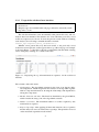
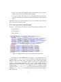
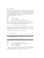
results have been requested, a table appears in the top of the web page. An example
is shown in Figure 1.1. The table is already sorted initially, but this initial ordering
can be changed by clicking on a column of the table.
Figure 1.1: Displaying the top 10 transformation sequences via the web-based
interface
The columns of the table mean:
• Configuration: The algorithmic structure in the form of an abstract skeletal configuration, which encapsulates the structure of the algorithm together
with its component information, showing the relationships and dependencies
among the components.
• Module, Function and Arity: The function, identified by the given M:F/A,
which contains the entry point of the algorithmic structure.
• Number of workers: The maximum number of workers required by this
transformation sequence.
• Expected speedups: After applying all the transformations, the tool predicts
that the analysed source can achieve these speedups. The prediction is based
on the measured sequential execution times.
5
• Recommended?: A transformation sequence is recommended if the analysed
source can accomplish either real CPU speedup or real GPU speedup by
applying the defined transformations. (Note that GPU estimates have not
been implemented so far.)
By clicking on the combo-box labelled Chart options, and selecting the
requested file format from the appearing local-menu, data export can be initiated.
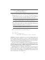
By clicking on a transformation sequence, its detailed view, containing all of
the transformation descriptions, appears in a table in the bottom of the web page.
An example is shown in Figure 1.2.
Figure 1.2: Detailed view of a transformation sequence
The columns of the table mean:
• Configuration: The algorithmic structure in the form of an abstract skeletal configuration, which encapsulates the structure of the algorithm together
with its component information, showing the relationships and dependencies
among the components.
• Location information: How to find the corresponding code fragments on
which the suggested transformation can be applied.
• Program text: The program text of the corresponding code fragment.
• Number of workers: The maximum number of workers required by this code
fragment after applying the suggested transformation.
• Sequential CPU/GPU times: The average of the measured execution times
of the corresponding code fragments.
• Parallel CPU/GPU times: After applying all the transformations, the tool
predicts that the corresponding code fragment can be executed within these
time bounds. The prediction is based on the measured sequential execution
times.
6
• Expected speedups: After applying all the transformations, the tool predicts
that the analysed source can achieve these speedups.
• Used stream length: The length of the stream with which the tool has measured the sequential execution times and has predicted the parallel execution
times.
This table can also be sorted by clicking on any of its columns, and its data can
also be exported in CSV file format.
1.2.4
Data types of the exported formats
In order to correctly import the CSV file, the following delimiters should be used:
• Text delimiter: ‘
• Field delimiter: ,
• Row delimiter: \n
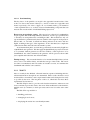
Figure 1.3: XML document exported from the web-based interface
A document exported in XML format (see Figure 1.3 for example) has a root
element, named tr_seq_entities, whose attributes hold the timestamp of the
XML generation and a hash value of the database contents. Each child element
of the tr_seq_entities container element corresponds to a transformation
sequence. These elements, named tr_seq_entity, have attributes that hold
the properties shown in the table of the transformation sequences. They also have
a child element, tr_comp_entities, which also acts as a container. Its child
elements, named tr_comp_entity, represent transformation descriptions. The
attributes of tr_comp_entity hold the properties that are shown in the table of
the detailed view.
7
Chapter 2
Implementation Details
2.1
UI workflow
The user interface of the ParaPhrase Refactoring Tool should be able to present
pattern candidates, i.e. code fragments amenable to parallelization by transforming into applications of skeletons. This presentation should be detailed enough so
that the user can make refactoring decisions upon, and it should be well-organised
so that unnecessary details and useless information do not prevent the user from
making good decisions. In particular, the user interface should filter out candidates
that are definitely worse than others, and prioritise the good ones.
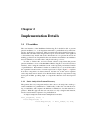
In order to achieve this, we have created software components that present
pattern candidates to users of the ParaPhrase Refactoring Tool on a web-based user
interface, after sorting the candidates based on the expected performance benefits
of parallelization. Performance benefits are estimated by a cost model that takes
the sequential execution time of certain expressions as input. Figure 2.1 explains
how these components are interconnected, and the rest of this section explains
each component in more details. Note that the Static Analysis component is being
developed in WP2, providing input to components that have been developed in
T4.2.
2.1.1
Static Analysis for Pattern Discovery
The pattern discovery component analyses the source code and points out the potential candidates for parallelization. Additionally, it takes into account the nesting of candidates, and computes the different combinations of transformation sequences. With this approach the user can select not only a single transformation,
but also transformation sequences for parallelization.
A simple example from the matrix multiplication module:
mult_seq(Rows, Cols) ->
lists:map(fun(R) ->
lists:map(fun(C) -> mult_sum(R, C) end,
8
Figure 2.1: Components to present pattern candidates to users
Cols)
end, Rows).
Possible options for transformation sequences are the following.
• Transform the top-level lists:map/2 application into a farm.
• Transform the inner lists:map/2 application into a farm.
• Transform both lists:map/2 applications, and obtain a farm of farms.
2.1.2
Cost Analysis
The pattern discovery phase finds source code segments that can be transformed
into applications of parallel skeletons, and generates combinations of those pattern
candidates that belong to the same code segment, and can be embedded into each
other. In other words, it identifies possible transformation sequences that could
result in parallelized code that uses the skeleton library.
The aim of the cost analysis component is to select transformation sequences
which are expected to result in significant speedup when comparing the execution
time of the original and the transformed (parallelized) code segment. Therefore,
during the cost analysis phase we measure the sequential execution time of code
segments, and calculate the parallel execution time using a cost model (Section
9
2.1.2.1). In some cases we also need to determine some missing input for the cost
model.
After the pattern discovery phase we have a list of transformation sequences. A
transformation sequence consists of transformation descriptions, where a transformation description describes which code segment could be transformed into which
kind of skeleton (for now we take into account only the farm and the pipeline
skeletons). In the cost analysis phase we process every transformation sequence
individually, and refine their transformation descriptions with some heuristic information:
• Estimated sequential execution time – the measured/calculated execution
time of the original code segment;
• Estimated parallel execution time – the predicted execution time after parallelization;
• Additional information for the transformation, for example the optimal number of workers in the case of a farm.
After we have extended all of the transformation descriptions in a transformation sequence, we highlight the outermost transformation, because its description
contains information concerning the whole sequence. This follows from the fact
that we calculate its parallel execution time assuming that all of the embedded
transformations will be applied. In the following we briefly introduce the calculation method of the heuristic information. The transformation description may
belong to either a map or a pipeline candidate.
Pipeline In the case of a pipeline candidate we need the number of stages, the
execution time of the stages and the length of the data stream as input for the cost
model. From the given code segment we identify the stages of the pipeline and ask
the benchmarking component (Section 2.1.2.2) to measure the execution time for
each. We also identify the expression that belongs to the data stream, and following
the dataflow in the source code, we try to estimate its length. If it is not possible, we
use a default stream length in the further calculations. After we have collected all
the needed information for the cost model, we can calculate the predicted parallel
execution time.
Farm In the case of a farm candidate we need the execution time of the function
that is applied to each element of the data stream, the length of the data stream
and the number of the workers as input for the cost model. From the given code
segment we identify the worker function, and ask the benchmarking component
to measure the execution time for it. We try to estimate the length of the data
stream similarly as in the case of a pipeline. The last step is to determine the
optimal number of workers: we calculate the parallel execution time for every
possible number of workers within a well-founded interval, and we choose the
worker number which results in the best execution time.
10
2.1.2.1
Cost Model
For the estimation of parallel execution time of Erlang expressions, we use a cost
model that has been derived from the cost models of the pipeline and the farm
skeletons already published by the ParaPhrase consortium [3, 4]. In order to make
our estimations more precise (namely, to cover implementation-level costs better),
we have slightly modified the published cost models. The cost model used for
evaluating pattern candidates is the following.
Pipeline
M
Tstages
Tcopy (L)
: the number of stages
: time costs of the stages (|Tstages | = M )
: time cost of sending L pieces of data between processes
The sequential execution time of calculating all the M stages on L pieces of data
takes L ∗ sum(Tstages ), while the same computation in parallel (assuming that we
have at least as many computing units as stages) will only take
sum(Tstages ) + (L − 1) ∗ max(Tstages )
time units. In the case of parallel execution, however, we need to deal with the
communication and process starting costs as well: setting up M workers and pushing every data item through the whole pipeline takes (Tspawn + Tcopy (L)) ∗ M extra
time units.
Therefore, we get the following time costs for pipelines:
Tseq := L ∗ sum(Tstages )
Tpar := sum(Tstages ) + (L − 1) ∗ max(Tstages ) + Tspawn + Tcopy (L) ∗ M
t i m e c o s t _ p i p e ( L , T _ s t a g e s ) −>
M = length ( T_stages ) ,
sum ( T _ s t a g e s ) + ( L − 1 ) ∗ max ( T _ s t a g e s )
+ ( t i m e c o s t _ s p a w n ( ) + t i m e c o s t _ c o p y ( L ) ) ∗ M.
Farm
Twork
Tcopy (L)
Np
Nw
:
:
:
:
time cost of the operation to be performed
time cost of sending L pieces of data between processes
number of computing units
number of workers started
In the case of algorithms transformable into the farm skeleton, the sequential
execution time of the computation on L elements is Twork ∗ L, while in parallel, we
can theoretically finish in Twork ∗ dL/min(Np , Nw )e time units.
11
t i m e c o s t _ f a r m ( N_p , N_w , L , T_work ) −>
T_work ∗ c e i l i n g ( L / min ( N_p , N_w) )
+ t i m e c o s t _ e m i t t e r ( N_w , L )
+ t i m e c o s t _ c o l l e c t o r ( N_w , L ) .
However, we have additional costs related to communication and process setup:
• Emitting takes Tspawn ∗ (Nw + 2) + Tcopy (L) ∗ 3 time units: spawning Nw
workers, the data source process and the emitter process, plus copying the
data to the data source, then to the emitter, and finally to the worker.
t i m e c o s t _ e m i t t e r ( N_w , L ) −>
t i m e c o s t _ s p a w n ( ) ∗ (N_w + 2 ) + t i m e c o s t _ c o p y ( L ) ∗ 3 .
• The collection of the results has two phases: the spawned collector process
receives the results from the workers, then it sends the data towards the final
destination. Formally, the cost is Tspawn + Tcopy (L) ∗ 2.
t i m e c o s t _ c o l l e c t o r ( _N_w , L ) −>
timecost_spawn ( ) + timecost_copy (L) ∗ 2.
That is, for the farm skeleton we get the following costs:
Tseq := Twork ∗ L
Tpar := Twork ∗ L/min(Np , Nw ) +
Tspawn ∗ (Nw + 2) + Tcopy (L) ∗ 3 + Tspawn + Tcopy (L) ∗ 2
Calibration Apparently, spawning and copy speeds may highly influence the
parallel execution time of skeletons. In order to compute reasonably accurate
costs, a calibration module has been integrated into the cost model. The calibration
checks both the process spawning and the heap copy speed of the actual machine.
Note that, for the moment, we have omitted GPU-related costs.
The copy operation is benchmarked as follows. We spawn a process whose
only purpose is to receive data, and send back an acknowledgement; then we generate lists with varying sizes (up to 128MB), and measure the time it takes to transfer the lists (10 times repeatedly, of which we take the average). The result of the
measurement is the microsecond/byte rate of the Erlang node.
Benchmarking the process spawning operation consists of measuring the time
needed for starting N/4, N/2 and N processes (10 times repeatedly, of which we
take the average). In this setting, N is the maximum number of processes that
can be spawned on the current Erlang node. The result of the measurement is the
microseconds needed to start a single process.
12
2.1.2.2
Benchmarking
The key factor of the parallel cost model is the sequential execution time of the
work to be done on the stream of data (Tstages and Twork in the case of pipelines and
farms, respectively). In order to supply our cost formula with a good estimation
of the sequential time cost, we have created a benchmarking component that can
measure the execution time of individual Erlang expressions.
Expression encapsulation, typing The expressions selected for benchmarking
are put together with all their dependencies (functions, records, type specifications)
so that they are encapsulated into an Erlang module. This module has only one
exported function, parametrised by the free variables of the expressions in question.
The module, on one hand, is turned into Erlang Abstract Code and is fed into
TypEr, resulting in the types of the arguments; on the other hand, we compile the
synthesised module and load it into the runtime system.
As an intermediate phase, we turn the type information returned by TypEr into
a QuickCheck data generator. We then apply the QuickCheck property based tester
as a systematic random generator for the free variables of the expressions to be
benchmarked: the values returned by the generator will be passed to the module
just compiled and loaded into the virtual machine.
Timing strategy We execute the function to be measured multiple times (at least
twice, at most one million times), and take the average of the results. The execution time is accumulated, and if it reaches at least 0.2 seconds, we terminate the
benchmark and calculate some statistics.
2.1.3
Web UI
After cost analysis has finished, all transformation sequences including their detailed transformation descriptions are determined. These results should be stored
and should be converted into such a representation that can be interpreted as easily
as possible by the users. The last phase of the tool, called Web UI, meets these
requirements and even more.
The Web UI prior aim is to provide a web-based user interface, where users can
browse and can export results. Due to the server-client architecture of the interface,
multiple users (for instance, a developer team) can browse its results at the same
time.
The Web UI is responsible for:
• handling persistence,
• managing its web server,
• displaying the results in a user-friendly manner.
13
2.1.3.1
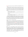
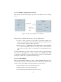
Building components of the Web UI
The data flow between the building components of the Web UI is shown in Figure 2.2.
Figure 2.2: Deployment diagram of the Web UI
The main tasks of the Web UI at the server side are detailed below.
• Persistence: This component is responsible for producing the final representation of transformation sequences. The transformation sequences stored
previously can be queried by other components.
• Provided services: A minimal web server, which needs no extra dependencies, is utilised transparently. This web server provides some web services
responsible for serving contents via separate protocols and handling user inputs.
Contents generated by one of the services are sent to the browser by the managed
web server via the HTTP protocol. These contents can be HTML pages, XML
or CSV files containing the exported transformation sequences or transformation
descriptions, JSON data or generated JavaScript scripts.
2.1.3.2
Used techniques
The Google Visualization API [1] provides a toolkit with which data can be presented to the user in various formats, for instance in a table with pre-defined actions
and style-sheets. The API has many built-in features and the ability to:
• query and display data in a formatted, fancy style;
• define an initial order for the displayed data;
• reorder the displayed data based on the user’s choice;
14
• decompose large amounts of data by displaying them page by page;
• handle user events, and
• export data in a user given format.
The API also gives the chance to use an own data source by implementing its
protocol. SQL-like queries can be sent via HTTP protocol to the data source to
retrieve data. It is important to note that no data is sent to Google, every data
manipulations are done within the client’s browser.
By utilising this API and implementing an own data source the results are displayed to the users in the web browser of the user. The implemented data source
can interpret requests defined by the query language of Google and can serve the requested contents in different formats (special JSON, CSV, XML, JavaScript script)
based on the request.
By handling user events, two tables can be shown in a joint view, where one
element of the first table can be detailed in the second table. Transformation sequences and their transformation descriptions can be visualised by applying this
joint view.
For other purposes, for example showing help dialogues to the users, jQuery [2]
is utilised. jQuery is a widely-used JavaScript framework, which allows the programmer to concentrate on real problems by hiding the differences in the behaviour
of different JavaScript engines. The programmer can choose from a wide variety
of DOM selectors, iterators, event listeners and so on.
2.2
Further improvements
Some of the features of the tool have not yet been completely implemented. Most
importantly, benchmarking is only performed on CPUs; benchmarking on GPUs is
under development.
For benchmarking an expression, we generate test data into its free variables.
Test data generation is implemented using QuickCeck, which needs type information on the data to be generated. Currently we compute the type of the free
variables with TypEr – this tool sometimes fails to find the appropriate type for
these variables: it finds a more general type than the one that could be used with
QuickCheck without running into a type error. We are currently working on some
improvements of the typing mechanism.
The cost model used for computing parallel execution time estimates from
measured sequential execution times only supports the pipe and the farm skeletons. Further skeletons will be added once pattern discovery will be able to return
those skeletons as well.
The tool is capable of displaying pattern candidates provided by the pattern
discovery component. However, this component (being developed in another work
package) has only an initial implementation. Improvements in this component will
have to be reflected in the other components of our tool.
15
Bibliography
[1] Google Visualization API Reference. https://developers.google.com/chart/intera
2013.
[2] jQuery - write less, do more. http://jquery.com/, 2013.
[3] C. Brown, M. Danelutto, K. Hammond, P. Kilpatrick, and A. Elliot. Costdirected refactoring for parallel erlang programs. International Journal of Parallel Programming, September 2013.
[4] C. Brown, V. Janjic, K. Hammond, M. Goli, and J. McCall. Bridging the divide intelligent mapping for the heterogeneous parallel programmer. ICPP’13,
2013.
16