1
ResearchContributions
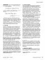
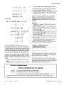
PROPOSITION 1. Let f be a real-valued function with
llfll = sup(f(j): j = 0, 1, 2, . . .) and P[L 5 N 5 R] z
1 - E. In exact arithmetic,
Proof. It suffices to show that cpO ] q(j) - p(j) ] I 2~
where q(i) = w(i)/W = p(i)//3 with @= p(L) + . . . +
p(R). Now
i I q(i) - A4 I 5 iL [4(i) - p(i)] + E
j=O
= igL p(i) i - 1 + E 5 2~. 0
[
I
For large X, our L is X - O(h) and our R is X +
O(A). This verifies that our overall work and space
complexities are both O(h). In contrast, the 1982 IMSL
routine asks the user to specify a parameter k-not
necessarily related to X-and outputs estimates of p(O),
p(l), . . . , p(k). This amounts to setting L = 0. The k
specified by any reasonable user will be O(X). Thus, in
practice the IMSL routine requires O(X) work.
1.1 Motivation
Gross and Miller [9] and Fox [4] consider problems of
this form, in which large values of X typically occur.
Given the f( j)‘s, the first summation in proposition 1
can be computed in O(A) time; without the left truncation, it would take O(X) time. For the terminalreward problem considered by Gross and Miller [6], the
required f( j)‘s can be computed in O(h) time using
successive (matrix) squaring up to L as Fox [4] details.
On the other hand, consider using the weights to compute Erlang’s loss formula (e.g., see Gross and Harris
with c servers as w(c)/[w(L) + . . . + w(c)] for L 5 c zz R.
If L = 0, the error is zero (ignoring roundoff and assuming no underflow occurs) but computing the weights
then takes O(X) time. For L > 0 we do not attempt a
formal error analysis here, which would require lower
as well as upper bounds on the left tail. Our bounds
may indicate a reasonable choice of R.
For another example, suppose that we want to
generate truncated Poisson variates by (efficientlyimplemented) inversion or by the alias method. Simply
scale standard uniform variates as u c uW and then
use the w (j)‘s directly. Our algorithm reduces the setup
time from O(X) for a naive method (with no error
bounds) to O(h) with bounds on truncation error. Fox
[5] bound the loss in coverage probability for confidence intervals constructed from truncated variates
with any distribution. Bratley, Fox, and Schrage [2] argue that truncation avoids statistical anomalies and allows variate generation by (efficiently-implemented)
inversion in O(1) marginal time, independently
of the
truncation point. Inversion is compatible with common
random numbers and antithetic variates, but rejection
methods typically are not.
April 1988 Volume 31 Number 4
1.2 Numerical Stability
The w( j)‘s are slightly inaccurate due to roundoff error.
They are all positive, so no cancellation errors occur
when adding them to get W. Thus, the additional roundoff error induced by adding the w(j)‘s is potentially
troublesome only when there are many summands
(large X). If we were simply to add from left to right say,
then for example w(f(m + R)/21) @ fi = I? in finiteprecision floating-point (@ = “add”) arithmetic for large
enough X. Here fi = w(L) + . . . + w(I(m + R)/21 - 1).
Thus, we will get W = fi though w(I(m + R)/21) + . . .
+ w(R) is not negligible. The cure is to add small weights
first. This widely applicable principle to attenuate roundoff error is also apparently used in the 1982 IMSL routine to compute Poisson probabilities.
Recursive computation of weights starting from the
mode is by itself not a new idea. What is new is its
coupling with a priori determination
of truncation
points and a priori underflow checks. The obvious
choice for w(m) is one. Given the computer’s underflow
and overflow thresholds, we typically choose w(m) far
larger to avoid underflow worries.
Knusel [lo, pages 1028-10291 gives a numericallystable method to compute p(i) for any fixed i, though he
gives no corresponding error bounds. It would be inefficient to use that method to compute the set of probabilities (p(L), . . . , p(R)]. He also gives a numerically-stable
method to estimate the masses in each tail with prescribed relative error. These bounds can be transformed
into corresponding bounds on absolute error. Whether
such transformed bounds are looser or tighter than ours
is an open question. Our bounds take O(1) time to compute, independently
of all other parameters. The time
and space complexities to compute Kniisel’s bounds are
unspecified and unclear. Our bounds on tail masses, as
estimates of them, probably would have high relative
error. In view of proposition 1, this seems irrelevant to
the applications cited above; in other applications, however, small relative error may be important. As a check
for programming errors, our w(m)/W should be approximately Kniisel’s estimate of p(m).
1.3 Overview
In section 2, we give an algorithm to find the weights,
which requires a subroutine to find L, R, and w(m) and
to check that underflow will not occur. We sketch that
subroutine in section 3, based on bounds in sections 4
and 5. Section 6 justifies the bounds in section 5. In
section 7 we outline generalizations to other discrete
distributions.
2. COMPUTING
WEIGHTS
In this section we present an easily-programmed
algorithm to compute the weights followed by an analysis
of roundoff error.
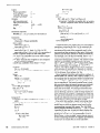
Algorithm. WEIGHTER
w(R), W, Fl
(X, E, 7, a; L, R, w(L), . . . ,
Communicationsof the ACM
441