Download fulltext - DiVA Portal

3 STRUCTURAL METHODS
This chapter describes the methods that are used in this thesis to find the parts of a model
useable to construct fault tests. This includes different forms of representing the structure of a
system and algorithms to find the desired subsets in a structural model.
As presented above, to construct a diagnostic system we need subsets of equations with
analytical redundancy. It is in general difficult to analytically find these subsets. In Krysander
(2006) it is formally shown that redundant parts can be found using structural methods. By
using structural methods, the problem can be transformed to graph theoretical problems for
which there exist efficient and well researched methods (Krysander, 2006). In structural
methods, only information about which variables that are present in which equations are
considered.
3.1 Structural models
To be able to perform structural methods we need a model to represent the structure of a
system. Such a model is called a structural model, and it will be used as input to the structural
methods. In this section two types of such models are presented.
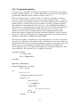
A structural model contains only information about which equation that contains which
variables. Consider the analytical representation of a system model:
e1:
e2:
e3:
dx1
dt
= − x12 + u
x2 = x12
y = x2
(3.1)
Here y and u are known, and x1 and x2 are unknown signals.
3.1.1 Matrix form
The structural model in matrix form corresponding to (3.1) is given in Table 3.1. An x in row
e1, column x1 means that variable x1 or its derivative is present in equation e1. A blank entry in
row e1, column x2 means that variable x2 is not present in equation e1. Known constants are
ignored.
Table 3.1 - Structural representation of equation system (3.1) in matrix form
Equation x1
e1
x
e2
x
e3
x2
x
x
u
x
y
x
3.1.2 Graph form
An analytical equation system can also be represented structurally as a graph. A graph
consists of nodes (or vertices), and edges joining them. In Figure 3.1, equation system (3.1) is
represented as a graph. In a graph, each edge has two endpoints. For example in Figure 3.1,
the edge ε1 has its endpoints in the nodes {e1, x1}. All of its variables and equations are
represented as nodes in the graph. There is an edge joining equation e to variable x if and only
if variable x or its derivatives are present in equation e. For example the node (or equation) e1
7