1
University of Illinois at Urbana-Champaign
Air Conditioning and Refrigeration Center
A National Science Foundation/University Cooperative Research Center
Exploratory Research on MEMS Technology
for Air Conditioning and Heat Pumps
T. M. Leicht, P. S. Hrnjak, and M. A. Shannon
ACRC CR-44
For additional information:
Air Conditioning and Refrigeration Center
University of Illinois
Mechanical & Industrial Engineering Dept.
1206 West Green Street
Urbana, IL 61801
(217) 333-3115
January 2002
The Air Conditioning and Refrigeration Center was
founded in 1988 with a grant from the estate of
Richard W. Kritzer, the founder of Peerless of
America Inc. A State of Illinois Technology Challenge
Grant helped build the laboratory facilities. The
ACRC receives continuing support from the Richard
W. Kritzer Endowment and the National Science
Foundation. The following organizations have also
become sponsors of the Center.
Alcan Aluminum Corporation
Amana Refrigeration, Inc.
Arçelik A. S.
Brazeway, Inc.
Carrier Corporation
Copeland Corporation
Dacor
Daikin Industries, Ltd.
Delphi Harrison Thermal Systems
General Motors Corporation
Hill PHOENIX
Honeywell, Inc.
Hydro Aluminum Adrian, Inc.
Ingersoll-Rand Company
Kelon Electrical Holdings Co., Ltd.
Lennox International, Inc.
LG Electronics, Inc.
Modine Manufacturing Co.
Parker Hannifin Corporation
Peerless of America, Inc.
Samsung Electronics Co., Ltd.
Tecumseh Products Company
The Trane Company
Valeo, Inc.
Visteon Automotive Systems
Wolverine Tube, Inc.
York International, Inc.
For additional information:
Air Conditioning & Refrigeration Center
Mechanical & Industrial Engineering Dept.
University of Illinois
1206 West Green Street
Urbana, IL 61801
217 333 3115
Abstract
This report presents an experimental investigation of refrigerant liquid mass fraction (LMF) in the exit
flows of plate evaporators. The objective is to identify a sensor that is capable of measuring small amounts of
refrigerant liquid in the superheated vapor at evaporator exits. This sensor should have the potential to be combined
with an active control scheme that increases the fill factor of the evaporator while simultaneously reducing superheat
temperature at the evaporator exit. Four methods were used to detect refrigerant droplets in the superheated vapor
stream exiting a plate evaporator: (1) an energy balance calculation, (2) a microfabricated thin-film resistance sensor
developed specifically for this project, (3) an exposed beaded thermocouple, and (4) photodiodes that detected laser
light scattered by droplets. The design, fabrication, calibration procedures, and theory of operation of the MEMS
thin-film resistance sensor are also presented in this report. Experimental results indicate that a MEMS thin-film
resistance sensor is more sensitive than a beaded thermocouple to LMF of non-equilibrium evaporator exit flows.
The MEMS sensor accurately detected refrigerant LMF as low as 1.5% in superheated evaporator exit flows.
iii
Table of Contents
Page
Abstract ......................................................................................................................... iii
List of Figures.............................................................................................................. vii
List of Tables ................................................................................................................ ix
Nomenclature................................................................................................................. x
Chapter 1: Introduction ................................................................................................. 1
Chapter 2: Experimental Facility .................................................................................. 3
2.1. Parallel plate evaporator test facility ...........................................................................................3
2.1.1 Refrigeration flow loop ..........................................................................................................................3
2.1.2. Water flow loop.....................................................................................................................................6
2.1.3. Test section............................................................................................................................................6
2.2. Instrumentation ..............................................................................................................................8
2.2.1. Pressure measurement ...........................................................................................................................8
2.2.2. Temperature measurement ....................................................................................................................9
2.2.3. Refrigerant mass flow measurement .....................................................................................................9
2.2.4. Power measurement...............................................................................................................................9
2.3. Laser Equipment ..........................................................................................................................10
2.4. Data Acquisition Hardware and Software..................................................................................10
Chapter 3: MEMS Resistance Sensors ...................................................................... 12
3.1. Overview .......................................................................................................................................12
3.2. Theory of Operation.....................................................................................................................12
3.3. Minimum Gap Serpentine RTD Design Equations....................................................................13
3.4. Design of Serpentine Resistors for Constant Heat Flux..........................................................14
3.5. Sensor Fabrication.......................................................................................................................16
3.5.1. General description..............................................................................................................................16
3.5.2. Microfabrication ..................................................................................................................................17
3.5.3. Packaging and installation in refrigerant piping ..................................................................................17
3.6. Sensor Calibration .......................................................................................................................18
3.6.1. 4-wire resistance technique .................................................................................................................18
3.6.2. In-situ calibration technique ................................................................................................................19
3.6.3. Comparison of results..........................................................................................................................22
Chapter 4: Experimental Procedures......................................................................... 25
iv
4.1. Experimental Scope.....................................................................................................................25
4.2. System Start-up and Operation ..................................................................................................25
4.3. Procedures for Methods of Calculating LMF ............................................................................26
4.3.1. Procedures and data collection ............................................................................................................26
4.3.2. Test envelope.......................................................................................................................................26
4.4. Procedures for Correlating Instrument Signals to LMF ...........................................................26
4.4.1. Procedures and data collection ............................................................................................................26
4.4.2. Test envelope.......................................................................................................................................26
4.5. Procedures for Characterizing Evaporator Exit Flows ............................................................27
4.5.1. Procedures and data collection ............................................................................................................27
4.5.2. Test envelope.......................................................................................................................................28
4.6. Procedures for Comparing Thermocouples and MEMS Sensors ...........................................28
4.6.1. Procedures and data collection ............................................................................................................28
4.6.2. Test envelope.......................................................................................................................................28
Chapter 5: Experimental Results ............................................................................... 29
5.1. Methods of Calculating LMF .......................................................................................................29
5.2. Correlating instrument signals to LMF......................................................................................32
5.3. Characterizing Evaporator Exit Flows .......................................................................................34
5.3.1. Introduction to experiments.................................................................................................................34
5.3.2. Case (1) - TXV control of a plate evaporator ......................................................................................34
5.3.3. Case (2) - MXV control of a plate evaporator .....................................................................................35
5.3.4. Case (3) – Controlled LMF with a two-evaporator arrangement.........................................................36
5.3.5. Performance of the MEMS sensor.......................................................................................................37
5.4. Comparison of thermocouple and MEMS sensor signals .......................................................41
5.4.1. Introduction to experiments.................................................................................................................41
5.4.2. Time domain analysis..........................................................................................................................42
5.4.3. Frequency domain analysis .................................................................................................................44
5.4.4. Effect of MEMS sensor surface area on sensitivity to droplets...........................................................44
Chapter 6: Conclusions and Recommendations ...................................................... 46
6.1. Conclusions..................................................................................................................................46
6.2. Recommendations .......................................................................................................................47
REFERENCES .............................................................................................................. 48
Appendix A. Calibrating the Thermocouple in the Glass Tube to Measure Vapor
Temperature................................................................................................................. 49
v
Appendix B. Procedures for Refrigeration System Startup.................................... 51
Appendix C: Summary of Runs 1-25 for Comparing Thermocouple and MEMS
Sensor Signals............................................................................................................. 52
vi
List of Figures
Page
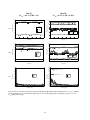
Figure 2-1. Photo of experimental facility ....................................................................................................................3
Figure 2-2. Flow schematic of experimental facility showing refrigerant lines (solid) and water lines (dashed).........4
Figure 2-3. Photo of evaporators, test section, and instrumentation .............................................................................5
Figure 2-4. Photo of the test section .............................................................................................................................7
Figure 2-5. Photo of instrumentation ............................................................................................................................9
Figure 2-6. Photo of the test rig, highlighting the calorimeter, laser, and static mixer ...............................................10
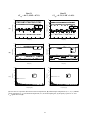
Figure 3-1. MEMS serpentine resistance sensors .......................................................................................................12
Figure 3-2. Dimensions of minimum gap serpentine resistors....................................................................................15
Figure 3-3. Microfabricated sensor with 3 serpentine RTD's .....................................................................................17
Figure 3-4. MEMS serpentine resistor calibration by 4-wire resistance method ........................................................19
Figure 3-5. Sensor voltage vs. current at two different vapor temperatures, T∞,1 and T∞,2 .........................................20
Figure 3-6 In-situ calibration of MEMS sensors at two temperatures, T∞,1 = 9.0°C (top), and T∞,2 = 14.3°C
(bottom) ...............................................................................................................................................................23
Figure 3-7. Comparison of MEMS sensor calibration techniques ..............................................................................24
Figure 5-1. Schematic of evaporators, static mixer, and test section instrumentation used to determine LMF...........30
Figure 5-2. P-h diagram of entrained liquid evaporating in a superheated vapor stream.............................................31
Figure 5-3. Comparison of LMF calculated from (1) direct measurement method, and (2) energy balance
method .................................................................................................................................................................31
Figure 5-4. Evaporator outlet thermocouple temperature Te,out, MEMS sensor temperature Ts,1, and scattered
laser light photodiode voltage in the presence of small quantities of liquid (LMF=0.41%)................................32
Figure 5-5. Normalized lock-in amplifier output of MEMS sensor and scattered laser light showing sensitivity
to droplets ............................................................................................................................................................33
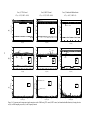
Figure 5-6. Evaporator outlet temperature signal comparison at low LMF during TXV control, MXV control,
and simulated maldistribution (a) during the entire run, (b) at 40Hz sampling rate, and (c) in the frequency
domain .................................................................................................................................................................38
Figure 5-7. Evaporator outlet temperature signal comparison at medium LMF during TXV control, MXV
control, and simulated maldistribution (a) during the entire run, (b) at 40Hz sampling rate, and (c) in the
frequency domain ................................................................................................................................................39
Figure 5-8. Evaporator outlet temperature signal comparison at high LMF during TXV control, MXV control,
and simulated maldistribution (a) during the entire run, (b) at 40Hz sampling rate, and (c) in the frequency
domain .................................................................................................................................................................40
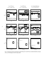
Figure 5-9. (T - Tsat) vs. liquid mass fraction behavior of thermocouples (Tmix, Te,out, Tvapor), and MEMS sensor
temperature (Ts,1) at three superheats 12°C (a), 10°C (b), and 8.6°C (c).............................................................42
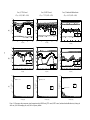
Figure 5-10 Thermocouple (Te,out), MEMS sensor (Ts,1), and scattered laser light signals in the time domain
(a), and frequency domain (b), for LMF = 0.28% (left), and LMF = 1.76% (right) ............................................43
Figure 5-11. Frequency spectra of the scattered laser light signal at low LMF (a), and high LMF (b). (low
LMF = 0.28%, high LMF = 1.76%) ....................................................................................................................44
vii
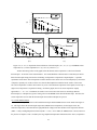
Figure 5-12. Effect of MEMS sensor surface area on signal frequency content for run 10; superheat = 10.0°C;
LMF = 0.32% ......................................................................................................................................................45
Figure A-1. Calibration of the thermocouple in the glass tube to measure vapor temperature...................................50
viii
List of Tables
Page
Table 3-1. Design parameters for the serpentine RTD’s.............................................................................................16
Table 3-2. Summary of MEMS serpentine resistor calibration by 4-wire resistance method.....................................18
Table 3-3. Summary of MEMS serpentine resistance sensor by the in-situ method. (T∞,1 = 9.0°C, and T∞,2 =
14.3 C) .................................................................................................................................................................22
Table 4-1. Test envelope for methods of calculating LMF .........................................................................................26
Table 4-2. Test envelope for characterizing evaporator exit flows ............................................................................28
Table 4-3. Test envelope for comparing thermocouples and MEMS sensors.............................................................28
ix
Nomenclature
Roman Symbols:
a
maximum serpentine resistor size
Acs
cross-sectional area
As
surface area of MEMS sensor
Co
MEMS sensor calibration constant
g
gap between serpentines in MEMS sensor
is
MEMS sensor current
l
active length of serpentine resistor
m1
initial slope of V1(is)
m2
initial slope of V2(is)
n
number of serpentines in MEMS sensor
LMF
liquid mass fraction
q& ′′
MEMS sensor surface heat flux
Rdesign
Ro
Rs
t
T
Tin-situ
To
Ts
Ts,1
Ts,2
Ts,3
Te,out
Tmix
Tsat
TTC
Τ4-wire
Τ∞,1
Τ∞,2
∆Tsup
Vs
V1
V2
w
design resistance of MEMS sensor
reference resistance at temperature To = 0°C
resistance of MEMS sensor
thickness of serpentine in MEMS sensor
Temperature
sensor temperature using in-situ calibration technique
reference temperature
MEMS sensor temperature
MEMS sensor temperature, large
MEMS sensor temperature, medium
MEMS sensor temperature, small
refrigerant temperature at main evaporator outlet
temperature at the static mixer outlet
saturation temperature
temperature measured by thermocouple in the glass tube
sensor temperature using 4-wire calibration technique
vapor temperature during sensor calibration
vapor temperature during sensor calibration
superheat temperature
voltage drop across MEMS sensor
sensor voltage at Τ∞,1
sensor voltage at Τ∞,2
width of serpentine in MEMS sensor
Greek Symbols:
temperature coefficient of resistivity {°C-1}
α
resistivity {µΩ-cm}
χ
x
Chapter 1: Introduction
Large heat pumps, refrigeration, and air conditioning systems often use plate heat exchangers (PHE) as
evaporators. Plate evaporators consist of multiple refrigerant channels, or plates, in which the refrigerant evaporates
vertically up each channel. Typically, the channels are connected in parallel, but they can also be circuited in a
serpentine fashion to achieve a desired performance level. In direct expansion (DX) systems, refrigerant is
expanded through a single throttling device such as a thermostatic expansion valve (TXV). TXV’s operate by
limiting the refrigerant flow so that the superheat temperature at the exit is high enough to ensure stable operation.
In horizontal tube evaporators, a superheat temperature of 5°C is usually enough for stability over a large range of
evaporator loads, but plate evaporators typically require superheats above 8°C for stable operation. A high
superheat degrades evaporator performance because it results in a large superheated zone in the evaporator where
heat transfer coefficients are lower than in the two-phase evaporating zone. Ideally, the evaporator should run with
zero superheat, for all evaporator loads, to maximize the two-phase heat transfer area of the evaporator. This is
impossible with DX systems using plate evaporators because distribution of the two-phase refrigerant is
complicated, and current distribution schemes using orifice tubes are unreliable. Multi-channel evaporators also
suffer from refrigerant side maldistribution caused by uneven loads within the evaporator. Flow maldistribution can
result in one or several channels being completely filled with two-phase refrigerant, while neighboring channels are
dry at the exit. Therefore, in plate evaporators, a high superheat is maintained to assure dry exit conditions and to
prevent large quantities of liquid from carrying over and damaging the compressor.
Since high exit superheat temperatures degrade evaporator performance and capacity, any refrigerant flow
control scheme that reduces the superheat required for stable operation will improve evaporator performance. A
good control strategy would include sensors that can detect a small liquid fraction in a superheated vapor stream,
and can be easily incorporated into a feedback loop with the throttling device. A further improvement to DX
systems using plate evaporators would be to incorporate these sensors with a multi-valve, active feedback flow
control strategy where refrigerant expansion can be independently controlled. Such a strategy could be realized by
using MEMS (microelectromechanical systems) flow control valves as the throttling device for each channel.
MEMS is an enabling technology that merges the capability to sense, actuate, and control the macro environment
with micro-scale systems. The technology has emerged from the fabrication processes of semiconductor devices,
and it is finding applications in the areas of 1) fluid sensing; 2) mass data storage; 3) optics and imaging; 4)
miniature analytical instruments; 5) biomedical sensors and many other areas. MEMS has the potential to provide a
small size, low power consumption, low mass, low cost, and highly functional solution to the problem of refrigerant
flow distribution within multi-channel evaporators. Of course, the same feedback control strategies could be
accomplished with normal scale valves, and the attendant sensors, circuitry, and controllers. These systems would
prove too bulky, expensive, and complex for controlling individual evaporator channels, and thus would not be
adopted by industry.
The purpose of this investigation was to measure the time-varying signals of several sensors at the exit of a
plate evaporator as superheat is decreased, and correlate those signals with a time-averaged liquid mass fraction
(LMF) in the superheated vapor stream. By investigating the sensor signals, it was possible to understand the nature
1
of the non-equilibrium two-phase flow exiting the plate evaporator. The time-averaged LMF of the evaporator exit
flow stream was measured by using a passive flow mixer to agitate the two-phase refrigerant mixture and evaporate
any entrained liquid droplets with heat supplied by the surrounding vapor. An energy balance of the inlet and outlet
flows through the mixer provides the time-averaged LMF.
The exit flows of three evaporator configurations were measured with a newly developed MEMS thin-film
resistance sensor, with a laser and photodiodes for measuring light scattered by entrained droplets, and with an
exposed beaded thermocouple. The evaporator configurations include 1) a plate evaporator fed by a thermostatic
expansion valve, 2) a plate evaporator fed by a manual valve, and 3) a two-evaporator configuration used to simulate
maldistribution between parallel channels. The MEMS sensor, scattered laser light, and thermocouple signals were
recorded at both slow and fast rates in order to characterize the unsteady flow exiting the evaporator. Results are
presented in the time and frequency domain, and indicate that as superheat is reduced, entrained droplet mists
emerge in regular intervals at the evaporator exit.
Three MEMS thin-film resistance sensors were designed, fabricated, and calibrated against known liquid
mass fractions for the purposes of this investigation. This report documents the general theory of operation of the
heated sensors, the methodology for designing thin-film serpentine resistors with minimum surface area, the
fabrication of the sensors on a thin silicon wafer, and the calibration of the sensors. The three MEMS sensors varied
in size, but all had the same surface heat flux. They were driven with a small constant DC current to provide selfheating in order to boil liquid droplets that would impact the sensor. A comparison of the three sensor signals in the
frequency domain reveals that the sensor size does not influence its ability to detect a small liquid mass fraction in a
superheated vapor stream.
The performance of the MEMS sensor and the beaded thermocouple when exposed to small liquid mass
fractions in a superheated vapor stream were compared. This was done to assess the feasibility of using each
instrument to control refrigerant flow to the evaporator by detecting and controlling LMF instead of controlling
superheat, as is the case of thermostatic expansion valves. A unique comparison of the DC and AC signals as a
function of LMF and superheat is presented for both instruments. Results show that the MEMS sensor is more
sensitive to LMF than the thermocouple. Both instruments exhibit a saturation point beyond which they can no
longer detect increases in LMF.
2
Chapter 2: Experimental Facility
2.1. Parallel plate evaporator test facility
A new refrigeration system was built for the purposes of this study in the Laboratory for Plate Heat
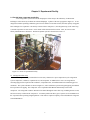
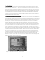
Exchangers at the University of Illinois in Urbana-Champaign. A photo of the test rig appears in Figure 2-1. It was
designed to simulate operating conditions typical of water chillers of less than 60 tons (210 kW) capacity using plate
heat exchangers for evaporation. The facility consists of three main parts: 1) the refrigerant loop, 2) the water loop,
3) and the evaporator exit test section. All of which will be discussed in this section. Later, in section 3.2 the
facility instrumentation is discussed. The data acquisition system is described in section 3.3.
Figure 2-1. Photo of experimental facility
2.1.1 Refrigeration flow loop
The refrigeration loop contained the four necessary elements of a vapor-compression cycle refrigeration
system: compressor, condenser, expansion device, and evaporator. In addition, there was a receiving tank for
collecting high pressure liquid from the condenser, a liquid subcooler, and instrumentation for monitoring process
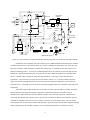
conditions. The system schematic is shown in Figure 2-2, where solid lines represent refrigerant piping, and dashed
lines represent water piping. The compressor was a Copeland model ZR61K2 hermetically sealed scroll
compressor. The refrigerant was R22. Mineral oil circulated through the entire flow loop, including the test section,
and was necessary to lubricate the compressor. A common problem in these types of systems is oil accumulation in
the evaporator when operating at high superheats. This reduces evaporator capacity, and could influence refrigerant
side maldistribution.
3
Condenser
Micro Motion
flowmeter
Subcooler
H2O Supply
Receiver
filter
to h.p.
cutoff
Micro Motion
flowmeter
Compressor
Expansion
Device
T2
bypass
MEMS
Valve
sight glass
T1,P1
metering
valve
T9
T5
to l.p.
cutoff
Secondary
Evaporator
DP
T4
Primary
Evaporator
T3
T10
H2O Res.
P2
T8,P4
Calorimeter
drain
T7,P3
T6
Mixer
MEMS
glass tube
HeNe Laser
Water •Pump
MEMS Droplet Sensor
Figure 2-2. Flow schematic of experimental facility showing refrigerant lines (solid) and water lines (dashed)
Immediately on the discharge side of the compressor was a SWEP model B15×60 parallel plate condenser.
Condensers like this one are often used in unitary A/C systems. Building cold water supply was used as the cold
fluid in the condenser, which operated in a counter flow arrangement. A manually set water flow control valve
adjusted condensing pressure. A receiver was installed downstream of the condenser to collect the high pressure
liquid before entering the liquid subcooler. The subcooler was also a SWEP design plate heat exchanger model
B8×20. A flexible, albeit complicated, water flow loop allowed for a wide range of achievable subcooled
temperatures. The water flow loop is discussed in more detail in section 3.1.2. Typically, building cold water
supply was circulated through the subcooler to provide a subcooled refrigerant temperature of 16°C before the
expansion device. Circulating cold water from the evaporator through the subcooler could attain colder subcooled
temperatures.
Subcooled refrigerant then divided into two branches, the main evaporator and the secondary evaporator.
This combination of the main and secondary evaporators constituted a parallel-pass evaporator in which
maldistribution could be induced by the user. Manual expansion valves fed both evaporators. Manual control
allowed the flow through each expansion valve to be precisely controlled such that the main evaporator operated
with high exit superheat, while the exit of the secondary evaporator was in the quality region. The exit streams
reunited prior to the test section such that the combined flows, superheated vapor from the main evaporator and high
quality refrigerant from the secondary evaporator, closely simulated the unsteady exit conditions of a plate
4
evaporator. The unsteady exit conditions of a TXV-controlled plate evaporator were first explored in a series of
tests using only the main evaporator.
The main evaporator, shown in Figure 2-3, was fed by an ALCO series TCL thermostatic expansion valve
that was modified for manual operation. The temperature sensing bulb and diaphragm assembly were replaced with
a micrometer handle attached directly to the valve stem cage assembly. The micrometer handle allowed for precise
control of evaporator feeding, and eliminated hunting problems associated with conventional TXV’s that add an
additional layer of complexity to multi-pass evaporator systems. Operating at a fixed expansion valve position also
permitted the investigation of evaporator dynamics, independent of TXV dynamics, over a wide range of superheat.
The main evaporator was a SWEP model B15×40 3-ton (10.5 kW) capacity parallel plate heat exchanger. It
consisted of 19 refrigerant passages and 20 water passages operating in a counter-flow configuration. The plates
had chevron style contours to enhance heat transfer. Two-phase refrigerant entered at the bottom of the evaporator,
evaporated vertically through the plates, and exited as superheated vapor at the top of the evaporator. The heat load
to the evaporator was supplied by water from the water reservoir. Thermocouples located immediately at the
entrance and exit of the refrigerant and water streams monitored process conditions. Care was taken to position the
exposed bead of the refrigerant exit thermocouple at the center of the exit pipe cross section.
Laser beam chopper
Secondary Evaporator
Test Section
Primary
Evaporator
Instrumentation
Expansion
Valve
Secondary
Flowmeter
Figure 2-3. Photo of evaporators, test section, and instrumentation
The secondary evaporator, shown in Figure 2-3, was somewhat unconventional because it was designed to
add only small amounts of high quality refrigerant to the test section. Flow rates through the secondary evaporator
from 0 to 1.5 grams/sec provided entrained liquid mass fractions (LMF) in the test section from 0 to 3%, depending
on main evaporator exit conditions. Since the flow rate was so low, and complete evaporation was not desired, the
secondary evaporator required a very small heat load. Sufficient heat could be generated, if and when needed, by
5
the ambient air such that a hot fluid (heat source) was not needed. The evaporator was simply a 12 inch long by ¼
inch diameter copper tube that had been brazed shut at one end. Then several small holes were drilled in that end
such that a uniform spray of high quality refrigerant could be injected into the test section along the streamwise
direction. A small needle valve with a micrometer handle served as the expansion device for the secondary
evaporator. Two thermocouples monitored the expansion process. One measured the subcooled liquid temperature
just upstream of the valve, and the other measured the saturation temperature within the evaporator tube.
2.1.2. Water flow loop
At the heart of the water loop, shown in dashed lines in Figure 2-2, was the 15 Liter (4 gallon) water
mixing tank. A Teel ½ hp centrifugal water pump pulled water from the bottom of the mixing tank, and pumped it
through the evaporator. Chilled water from the evaporator then recirculated back to the mixing tank. At the same
time, some of the hot condensing water was diverted into the mixing tank. The hot condensing water and chilled
water from the evaporator mixed in the tank to provide the appropriate inlet water temperature for the evaporator.
Water flow rate was controlled via a bypass line and throttling valve connected between the pump discharge and the
mixing tank. A drain hose located 20 cm above the bottom of the tank kept the water level in the mixing tank
constant.
The water flow loop was flexible enough to provide a wide range of subcooled refrigerant temperatures
from 4 to 25°C. There were two ways the water loop could be configured in order to achieve this range. First,
building cold water supply could be routed directly through the subcooler and on into the drain. This provided a
functional range of 12 to 25°C. Second, a small percentage of chilled water from the evaporator could be routed
through the subcooler to reach the lower end of the range from 4 to 12°C. For all of the runs conducted in this study
the target subcooled temperature was 16°C, so building water was always used in the subcooler.
2.1.3. Test section
The test section consisted of a laser section, the MEMS resistance sensor, a glass tube for flow
visualization, a static flow mixer, a calorimeter, and several thermocouples and pressure transducers for monitoring
flow conditions. The unsteady mixture of superheated vapor and entrained liquid droplets from the evaporators first
passed through the laser section. It consisted of a 2.0 mW Helium-Neon laser, a light chopper, and two photodiodes.
The light chopper and other related laser instrumentation are discussed in section 3.3. The laser, shown in Figure 26, was aimed through an optical window perpendicular to the flow. Some of the beam was scattered by refrigerant
droplets, and the rest passed through the flow stream unaffected. The unaffected laser light was collected by a
photodiode positioned directly across the flow stream along the laser axis. A portion of the scattered beam was
collected by a second photodiode located above the flow centerline, as seen in Figure 2-4. The entrained refrigerant
droplet volume can be measured from these two photodiode signals
6
Scattered Light
Photodiode
MEMS Sensor
Circuitry
Pressure
Transducer
Secondary
Evaporator
Thermocouple in
glass tube
MEMS Sensor
between flange
Primary
Evaporator
Figure 2-4. Photo of the test section
After the laser section, the flow encountered the MEMS resistance sensor. The sensor was mounted
between two glass plates and then installed into a flange in the test section piping. A detailed discussion of the
sensor design, fabrication techniques, and theory of operation is left for Chapter 4.
After passing the MEMS sensor, the flow entered a 5” long x 1” OD glass tube. The glass tube allowed for
evaporator exit flow visualization. A thermocouple (beaded type) was inserted into the tube through a ¼ inch
diameter glass tube (forming a tee). The thermocouple was secured with a compression fitting using Teflon ferrules,
allowing the position of the thermocouple to be adjusted. This was desirable because under certain flow conditions
having a high liquid mass fraction, splashing liquid would submerse the thermocouple causing drastic drops in the
sensed evaporator exit temperature.
Next was the static mixer. It is shown in Figure 2-6, along with the calorimeter. The mixer was designed
to stir the flow such that all of the entrained liquid was completely evaporated by the surrounding superheated vapor.
Provided liquid was present, conditions at the exit of the mixer would be uniformly superheated at a temperature less
than the original superheat temperature. Pressure drop in the mixer was marginal, and has been measured at no
more than 3 kPa during conditions of interest. The static mixer consisted of a 6 inch long by 2¼-inch diameter
copper tube with a helical copper sheet inside. The helix provided enough mixing to allow LMF measurements as
much as 5%.
To directly measure the quality of the evaporator exit fluid, a calorimeter for measuring refrigerant
entrained mass fraction completed the test section. It should be noted that the calorimeter was not used in this
capacity for the majority of test conditions performed in this study. The calorimeter consisted of a 3,450 Watt
Chromalox finned tubular heater inserted into 1-3/8 inch OD copper tube. The heater was 48 inches long with 4½
fins per inch. The calorimeter was well insulated, and was instrumented with thermocouples and pressure
transducers at the entrance and exit. Heater power could be conveniently adjusted by a variac, and the power output
was measured directly with a watt transducer. The thermocouples, pressure transducers, and watt transducer are
7
detailed in the next section. The calorimeter served two purposes. First, when the system was running with
relatively little liquid at the evaporator exit the heater was used to ensure that all of the liquid had been evaporated
before entering the compressor. Second, the calorimeter could be used when the evaporator is fully wetted to
measure exit quality.
2.2. Instrumentation
The refrigeration flow loop has been instrumented to measure refrigerant mass flow, pressure, temperature,
calorimeter heater power, laser light intensity for Mie scattering experiments, and MEMS sensor voltages. Each
type of measurement is discussed separately in this section. This includes the particular equipment used, any
calibration procedures performed, and an assessment of measurement uncertainty.
2.2.1. Pressure measurement
Three absolute pressure transducers, one differential pressure transmitter, and one gage pressure transmitter
were used to monitor refrigerant flow conditions. The location of these sensors is indicated in Figure 2-6. A
Sensotec 0 to 500 psia (0 to 3,450 kPa) absolute pressure transducer was located in the subcooled refrigerant line
before the expansion valve of the main evaporator. The evaporating pressure and the static mixer exit pressure were
measured by two Sensotec 0 to 200 psia (0 to 1,380 kPa) absolute pressure transducers. All three Sensotec
transducers had a 0 to 5 VDC output and a reported accuracy of ±0.1% of the full scale reading. Since these
transducers were newly purchased, the factory calibration factors were used during data collection. The main
evaporator differential pressure was measured by a Setra 0 to 2 psid (0 to 13.8 kPa) differential pressure transmitter.
It had a 4 to 20 mA output, so a 250 Ohm resistor was used at the backplane of the multiplexer to convert the current
output to the standard 0 to 5 VDC. A Setra 0 to 250 psig (0 to 1,720 kPa) gage pressure transmitter measured the
calorimeter exit pressure. It had a reported accuracy of ±0.13% of the full scale reading at constant temperature.
Since this transmitter measured gage pressure, it was necessary to record the barometric pressure during each day of
data collection. The barometric pressure was measured with a Princo Instruments 20 to 32 inHg (67.7 to 108 kPa)
mercurial barometer. It should be noted that the differential pressure transmitter and the gage pressure transmitter
were both calibrated in-situ against the Sensotec pressure transducers.
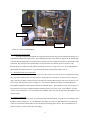
8
Voltmeters
Oscilloscope
Wave Generator
Lock-in
Amplifiers
Figure 2-5. Photo of instrumentation
2.2.2. Temperature measurement
All of the temperatures throughout the refrigerant and water flow loops were measured with Omega type T
ungrounded beaded thermocouple probes. The beaded thermocouples were chosen, as opposed to the shielded type,
so that the thermocouple junction would be directly exposed to the flow conditions and a faster response time could
be attained. This was especially important in the test section where fast, unsteady processes occurred. The
thermocouples were calibrated, along with the measuring system, over a range of 0 to 30 °C in an isothermal bath
against NIST traceable thermometers. The estimated uncertainty of the thermocouples is ±0.1°C.
2.2.3. Refrigerant mass flow measurement
Two Micro Motion ELITE coriolis effect mass flow sensors were used to measure refrigerant mass flow
rates. The main evaporator flow was measured by a model CMF025 sensor with a 0 to 40 lb/min (0 to 300 g/sec)
range, while the secondary evaporator flow was measured by a model CMF010 sensor with a 0 to 3 lb/min (0 to 23
g/sec) range. Both flowmeters, shown in Figure 2-3, were used in conjunction with their own model RTF9793
Field-Mount Transmitter, which outputs both flowrate and fluid density. The transmitters can be seen in Figure 2-6.
The flowmeters were factory calibrated and had a reported accuracy of ±0.10% of F.S. ±[zero stability ÷ flowrate
×100]% of the measured rate. The zero stability of the CMF025 sensor was 0.001 lb/min and for the CMF010 it was
0.00015 lb/min.
2.2.4. Power measurement
The calorimeter heater power was measured with an Ohio Semitronics 0 to 4 kW (0 to 13,600 Btu/hr) watt
transducer, shown in Figure 2-6. It was calibrated in situ against two Fluke 4.5 digit multimeters; one measuring
voltage across the heater and the other wired as an ammeter measuring heater current. The watt transducer has a
reported accuracy of ±0.04% of the full scale reading.
9
Transmitters for Flowmeters
Variac
Watt Transducer
Test Section
Laser
Static Mixer
Calorimeter
Figure 2-6. Photo of the test rig, highlighting the calorimeter, laser, and static mixer
2.3. Laser Equipment
Figure 2-5 and Figure 2-6 show the laser and related instrumentation used in the test section to identify the
presence of entrained liquid droplets. The hardware included a 2.0 mW Helium-Neon laser and power supply, a
light chopper, two photodiodes, and two ThorLabs lock-in amplifiers. The light chopper was a 4 inch diameter
windmill-shaped disk having 10 blades that “chopped” the beam at a user specified frequency. The laser beam was
directed through the test section pipe, perpendicular to the flow direction. A portion of the laser beam was scattered
by entrained liquid droplets. Some of the scattered light was collected by the photodiode located 3 inches above the
flow centerline. The unscattered portion of the laser beam was either absorbed by the refrigerant, or passed through
unaffected to the second photodiode located across from the laser. The photodiodes output a voltage signal
proportional to the collected light intensity, and these signals were routed through coaxial cable to a pair of lock-in
amplifiers. The lock-ins can either output the unamplified photodiode signal through their monitor outputs, or they
can throw out unwanted frequencies, and noise, by comparing the photodiode signal to a reference signal. If a
reference signal is used, which for our case was the chopper frequency, then the lock-in will filter out all frequencies
in the input signal except that of the reference signal. In this way, the lock-in is an extremely powerful tool for
filtering noise from the photodiode signal.
2.4. Data Acquisition Hardware and Software
The data acquisition hardware included a Gateway Pentium P5-133 MHz personal computer (PC)
connected via standard HP-IB interface to a Hewlett-Packard (HP) 1300A B-size VXI Mainframe. The mainframe
housed a HP E1326B 5 ½ digit multimeter, a HP E1345A 16 channel relay multiplexer, a HP E1347A 16 channel
10
thermocouple relay multiplexer, and a HP1353A 16 channel thermocouple FET multiplexer. The multimeter and
the three multiplexer boards were arranged in a scanning digital multimeter configuration. The HP equipment was
purchased because it provided
1.
High measurement accuracy down to the micro-volt range, in particular for unamplified
thermocouple voltages,
2.
High speed temperature measurements up to 100 K switches per second with the FET multiplexer,
and
3.
Convenient measurement of DC voltage, RMS AC voltage, 2-wire resistance, 4-wire resistance,
and temperature (thermistors, RTD’s, thermocouples).
All data acquisition programming was done using the HP-VEE (Visual Engineering Environment)
version 3.21 software program. HP-VEE is a general purpose, high level, iconic programming environment
similar to National Instruments LabView. The software provides features for instrument control, data acquisition,
data processing data analysis, and file management.
11
Chapter 3: MEMS Resistance Sensors
3.1. Overview
This chapter describes the efforts of this study to design, manufacture, calibrate, and test a MEMS
resistance sensor to be used in conjunction with micro-valves for controlling parallel plate evaporators in
refrigerators and heat pumps. The MEMS sensor is actually three sensors in one. It consists of three separate
serpentine nickel (Ni) resistors that are evaporated on a silicon wafer 250 µm thick. The serpentine resistors, shown
Figure 3-1, are very thin (~1000 Angstroms) and measure 0.0625 mm2, 0.25 mm2, and 1.0 mm2 in total surface area.
Since this will be the first generation of MEMS sensors, it is advantageous to have three sensors on the same
substrate in order to compare the effect of sensor size (surface area) on sensitivity to liquid droplets. A constant DC
current, in the milli-amp range, passing through the sensors provides i2R self-heating, so that a droplet will
evaporate when it strikes the sensor. The evaporation of droplets on the sensor surface causes the sensor
temperature, and resistance to decrease. It is important that the thermal mass of the resistors is extremely small to
give a very fast time response to refrigerant droplets impinging on the surface. Experiments were conducted to
measure the time-varying voltage signal of each sensor while exposing the sensors to known liquid fractions in a
superheated vapor. The sensor output signal can be correlated in both time and frequency domains with
thermocouple signals, laser light intensity scattered by the entrained liquid droplets, and the time averaged liquid
mass fraction.
Sensor 2
Sensor 1
Sensor 3
2 mm
Figure 3-1. MEMS serpentine resistance sensors
3.2. Theory of Operation
At high superheats, or evenly distributed evaporator flows, the sensor will work much like a hot wire
anemometer, where the self-heating will cause the actual sensor temperature to be elevated above the free stream
temperature. The extent to which the sensor temperature is higher will depend on the sensor current, the
temperature coefficient of the sensor, α [°C-1], the convective heat transfer coefficient between the sensor and the
free stream, and the free stream temperature. With the presence of liquid droplets the story becomes a little more
12
complicated. Initially, as small amounts of droplets strike the sensor they will be evaporated by the i2R sensor heat.
As more and more liquid coats the sensor, the sensor temperature is driven lower, until the sensor is completely
saturated and can no longer evaporate droplets before the next one strikes. When the sensor is completely wetted
there is a thin film of boiling liquid covering the surface, so the sensor temperature will approach Te, the excess
temperature above the saturation temperature of the boiling liquid required to drive the boiling process. Thus, at any
given time the sensor temperature can vary from an upper limit above the free stream vapor temperature to a lower
limit of Te, which is slightly greater than Tsat determined at the evaporator exit pressure. What this means from a
control viewpoint is that one sensor alone, located in the evaporator outlet pipe, can not provide an accurate measure
of superheat, especially when liquid is present due to maldistribution. In which case it might be advantageous to use
a second sensor in a location where it would be sheltered from droplet impingement in order to measure the vapor
temperature, and determine superheat.
3.3. Minimum Gap Serpentine RTD Design Equations
The smaller we can make the sensor, while maintaining a high degree of functionality with regard to
temperature accuracy and liquid detection capability, the more economically viable the technology becomes. It is
important to remember that ultimately these sensors are to be ganged together so that the outlet state of each
refrigerant channel can be measured. In plate heat exchangers the refrigerant passes are typically not more than a
few millimeters wide. This puts a constraint on the allowable physical size of the sensor. The RTD sensors
designed and built for this study are a thin metal film that serpentines back and forth within a square outline. The
idea is to design the sensor with a minimum gap between serpentine lengths so that a long resistor can be compacted
into the smallest possible surface area. Figure 3-2 shows the general shape of the sensors used in this study, with the
important dimensions labeled symbolically. There are six parameters (shown in Figure 3-2) that define the sensor
geometry, and only four of those six are necessary to complete a design (we choose g, n, t, and w). A further
constraint is that the number of serpentine lengths, n, must be an integer. Therefore, it is common practice for the
designer to select n as one of the four necessary parameters, based upon the desired final size and active length of
the sensor. The sensors used in this study are the minimum gap type, so the gap, g, is the second necessary
parameter in the design. The minimum gap is a function of the resolution attainable during the photolithography
process. Masks made by the University of Illinois’ Office of Printing Services produced, at best, a 15 µm gap.
These masks were made on transparencies from postscript files generated from original AutoCAD drawings of the
sensors.
What is important to the designer is the overall size of the sensor. This will influence the active sensor
length, the sensor’s ability to detect small liquid droplets, and the feasibility of packaging multiple sensors within
plate heat exchangers. The maximum serpentine RTD size is
a = n( w + g) − g = nw + ( n − 1) g
(3.1)
Another key parameter in the sensor design is the active length, l. The active length is defined as the total centerline
length of the serpentine resistor. For long RTD’s with many serpentine passes (n > 10), or RTD’s with a large
aspect ratio (l/w > 100), the centerline approximation gives a reasonably accurate estimation of the true active
13
length. However, for RTD’s with few serpentine passes (in the case of our smallest sensor, n = 2), or small aspect
ratios, this approximation breaks down because electric current always flows in the path of least resistance. In other
words, a larger percentage of the current will flow along the inner corners of the serpentine, rather than along the
centerline and the outer corners. Keeping with the centerline approximation, the active sensor length can be written
as
l = n( a − w ) + w + ( n − 1) g + ( n − 1) w
(3.2)
l = na + ( n − 1) g
(3.3)
Combining this result with eq. (3.1) and simplifying gives the active length in terms of the design variables g, n,
and w
l = n 2 ( w + g) − g
(3.4)
3.4. Design of Serpentine Resistors for Constant Heat Flux
For simplicity, and to aid in comparing the effect that sensor size has on its ability to detect entrained
liquid, the three serpentine resistors were designed to have equal surface heat flux. The resistance of the serpentine,
assuming constant temperature throughout the active sensor length, is
Rs =
χl
A cs
(3.5)
where Acs = wt is the cross-sectional area of the serpentine, and χ is the resistivity of the metal film. The bulk value
of resistivity for nickel given in the literature χ = 6.84 µΩ-cm has been used in this design [1]. The heat flux per
unit surface area of the sensor is
q& ′′ =
i s2 R s2
As
(3.6)
where is is the sensor current, and As is the surface area which can be expressed in terms of the design variables g,
w, and n
{
}
A s = wl = w n 2 ( w + g) − g
(3.7)
The concept of the sensor is to be able to evaporate, and detect individual liquid droplets. Barnhart has employed
P/DPA laser diagnostics to measure average droplet diameters of 50 microns after the dryout point of horizontal tube
evaporators [2]. This serves as a good starting point for designing the MEMS sensors. The power required to
evaporate a 50 µm diameter droplet of refrigerant R-22 is 0.017 mW. As an upper bound, assume the maximum
droplet diameter is 500 µm, an order of magnitude larger. The maximum power for evaporation would be 17 mW.
This assumes that a droplet will fully wet the sensor surface, and be fully evaporated before the arrival of another
droplet.
14
10w minimum
a
w
g
w
a
l
2w
i=1 i=2
i=3 ...
i=n
a = maximum size of the RTD
g = gap
l = active resistor length
n = number of serpentines (integer)
t = thickness (into the page)
w = width of serpentine
Figure 3-2. Dimensions of minimum gap serpentine resistors
The allowable size of the sensor is dictated by plate evaporator geometry and the mechanisms of droplet
evaporation. Plate geometry provides an upper limit to the sensor size of around 1 mm2. If the sensor were any
larger, it would be impossible to install within the plate outlet. Droplet evaporation provides the lower bound on
size. It is probably safe to assume that entrained droplets indeed have a characteristic dimension of 50 µm. A
sensor that is smaller than the smallest characteristic dimension of a droplet would be unable to distinguish between
small and large droplets, because every droplet in the flow stream would be capable of fully wetting the sensor
surface. Thus, the characteristic sensor dimension, a, of the three sensors was selected to span the range of 50
microns to 1 millimeter. Specifically, we tried to target 1, 0.5, and 0.15 mm for the characteristic size of the three
15
sensors. Two of the other key sensor dimensions, g and t, were determined by microfabrication constraints. The
gap, g, should be as small as possible to keep the sensor size small. Our microfabrication process yielded a 25 µm
minimum gap. Thickness, t, also needs to be small to reduce the sensor thermal mass. A thin layer of nickel, 1000
o
A thick, was placed on the silicon substrate to form the serpentine resistors.
With g, and t fixed by microfabrication constraints, and the approximate size, a, given for each sensor, we
only need to determine the serpentine width, w, of the serpentine. In order to do this, the nominal sensor resistance
must be set such that when a small DC current is applied to the sensor, the voltage drop is in the range of 1 to 5
VDC. A majority of instruments and transmitters have outputs in this range, so signal amplification would not be
necessary, and the signal could be read directly with a multimeter. To keep power requirements of the sensor to a
minimum, the design current should be in the range of 1 to 25 mA. Using Ohm’s Law with a 25 mA current and 5
VDC voltage drop gives a sensor resistance of 100 Ω. Assuming this will be the design resistance for the largest
resistor (a = 1 mm), then the heat flux per unit area will be
q& ′′ = 62.5 kW/m2 when the current is 25 mA. Given the
target dimensions, surface heat flux, and design current, the designer can apply eq. (3.2) to (3.7) and iterate to
determine the final values of the four key parameters g, n, t, and w. Table 3-1 summarizes the final design
parameters of the three serpentine resistors that were made for this project. It should be noted that the values in the
table are design values only, and should not be taken as exact quantities. The actual size of the sensors is
determined by the resolution of the microfabrication process, so each sensor needs to be calibrated to determine
precisely the reference resistance. However, in future calculations requiring sensor dimensions, the values in the
table will be used because they are within reasonable accuracy for our purposes.
Table 3-1. Design parameters for the serpentine RTD’s
2
sensor
a [µm]
n
g [µm]
w [µm]
l [µm]
As [mm ]
Rdesign [Ω]
1
2
3
975
483
189
10
5
2
25
25
25
75
76.5
82
9975
2513
403
.748
.192
.033
91.0
22.9
3.67
q& ′′
2
[W/m ]
122 - 76k
119 - 74.6k
111 - 69.5k
3.5. Sensor Fabrication
3.5.1. General description
A thin rectangular silicon wafer is the foundation of the MEMS sensor. On it are the three serpentine Ni
resistors, two thick gold current leads, and 6 thin gold voltage leads. Two of the voltage leads are unused, and were
added solely to provide redundancy in case a problem arose during fabrication. The sensors are suspended in the
middle of the flow stream by four narrow silicon bridges that have the full thickness of the wafer. The bridges in
earlier sensor generations were as thin as 40 µm, but that proved disastrous as the thin bridges were not strong
enough to withstand the flow in the test section pipe. These features are highlighted Figure 3-3, which shows the
complete MEMS sensor after microfabrication. Immediately behind the sensors, the silicon has been etched back to
a thickness of only 40 µm. This helps minimize heat conduction losses through the substrate, and assures that most
of the self-heating is dissipated by convection to the surrounding vapor and conduction to liquid droplets boiling at
the surface.
16
3.5.2. Microfabrication
For a detailed description of the microfabrication techniques used to produce the sensors, the reader is
directed to the work of Shannon et al. [3]. The specifics of microfabrication are relevant to this project only with
regard to the constraints that fabrication techniques placed on the sensor design. This study is not concerned with
the impact and contribution that the sensor fabrication techniques have to the world of MEMS. Rather, this study
views the MEMS sensor as a potential tool with which to measure and control maldistribution in multi-channel
evaporators. It is the intent of this project to assess the feasibility of using these devices to realize a sensing, and
actuation strategy for multi-valve flow control.
3.5.3. Packaging and installation in refrigerant piping
The prototype MEMS sensor is very large, at least with respect to the typical scale of most MEMS devices.
It is also flat, brittle, and much too delicate to be directly inserted into the refrigeration piping. In an effort to protect
the sensor from catastrophic fracture during service, it has been mounted in a “sandwich” between two pieces of ¼”
thick plate glass. A thin sheet metal plate having the same rectangular shape as the wafer is placed within the
sandwich to help support the silicon bridges exposed to the refrigerant flow. First, a two-part epoxy is spread
evenly, and extremely thin, across one of the pieces of glass using a razor blade. The sheet metal is placed on this
piece of glass and allowed to dry. Then another thin layer of epoxy is spread over the sheet metal and glass. The
sensor is carefully placed in exact alignment over the sheet metal support plate. At the same time a thin layer of
epoxy is laid over the second piece of glass, and then placed in contact with the sensor. The sandwich is clamped in
a specially designed fixture and left to harden for 24 hours. Once the epoxy has set, the sensor is mounted within
the test section in a copper pipe flange. Two o-rings in the flange provide a pressure tight seal against the glass.
Certainly, other less fragile materials besides glass plate could have been used to create the sandwich. However,
glass was selected because it is transparent which allows the entire wafer to be inspected after the epoxy has
hardened. This proved to be very useful, since several sensors were rendered useless after uneven clamping in the
flange caused complete cracking of the silicon wafer.
Figure 3-3. Microfabricated sensor with 3 serpentine RTD's
17
3.6. Sensor Calibration
3.6.1. 4-wire resistance technique
The principle of operation of a serpentine resistor is the fact that the resistance to the flow of electricity is a
function of the cooling due to the surrounding vapor stream (and possibly entrained liquid). The resistance as a
function of sensor temperature, Ts, can be expressed as
(
)
R s = R o 1 + α(Ts − To )
(3.8)
where Ro is the resistance at the reference temperature, To = 0°C, and α [°C-1] is the temperature coefficient of
resistivity. Since α is a constant material property in the range of temperatures of interest to refrigeration, eq. (3.8)
reduces to the following linear relationship for Rs(T)
R s ( T) = R o + αR o T
(3.9)
The above equation provides a basis for calibrating the sensor. The reference resistance Ro is simply the y-intercept
of Rs(T), and αRo is the slope. The calibration is complete when α and Ro have been determined for each of the
three serpentine resistors.
An experiment for calibrating α and Ro for each serpentine resistor was carefully performed over several
days. The complete MEMS sensor and a calibrated type-T beaded thermocouple were exposed to 3 different
temperatures in order to develop the Rs vs. Ts data. The 3 temperatures were achieved by placing the sensor and
thermocouple in (1) ambient conditions, (2) a 3 cubic-ft refrigerator, and (3) the freezer compartment of the
refrigerator. The sensor was exposed to each temperature for a period of 24 hours to ensure equilibrium conditions
were reached. Sensor resistances were measured with the HP 5 ½ digital multimeter using a 4-wire technique. To
minimize any self-heating of the resistors during the 4-wire measurements it is necessary to keep the source current
to a minimum. The effect of self-heating can be minimized by selecting a higher resistance range on the multimeter
since less current is applied. However, higher ranges yield lower resolution. It was determined that the default
setting of the multimeter (16384 Ω range, and 61 µA) was adequate to prevent self-heating and still provide ± 15mΩ
resolution (see p.87 in [4]). The results of the calibration are presented in Table 3-2.
Table 3-2. Summary of MEMS serpentine resistor calibration by 4-wire resistance method
MEMS
sensor
nominal surface
area,
A [mm2]
Rs1
Rs2
Rs3
average
1.0
0.25
0.0625
reference
resistance at
To = 0°C,
Ro [Ω]
107.03
27.51
5.01
18
temperature
coefficient of
resistivity,
α [°C-1]
.0045
.0044
.0043
.0044
140
120
R1 = (0.482)T + 107.03
2
R = 0.999
Resistance [Ω]
100
80
60
R2 = (0.121)T + 27.51
2
R =1
40
20
R3 = (0.0214)T + 5.01
2
R =1
0
-5
0
5
10
15
20
25
30
Temperature [°C]
Figure 3-4. MEMS serpentine resistor calibration by 4-wire resistance method
The average temperature coefficient of resistivity for the three resistors was found to be 0.0044 °C-1. Since
α is a constant material property, this average value will be used for all three resistors in future calculations. Bruun
reports a typical value of α20 = 0.0038 °C-1 for platinum hot-wire elements at room temperature (20°C) [5]. Our
thin-film serpentine resistors show a 16% improvement in temperature sensitivity compared to platinum hot-wire
anemometers.
3.6.2. In-situ calibration technique
An in-situ calibration of the sensors was also performed. The in-situ method has the advantage of
accounting for any errors in the sensor temperature measurement that might be introduced by the data acquisition
system. This method provides a means of determining sensor temperature, Ts, directly from voltage and current
measurements, without relying upon explicit knowledge of α, Ro, and To. To perform this calibration, the sensor
was installed in its mounting flange in the test section exactly as it was during normal operation. This means using
the same wiring to the current source, the ammeter, and the HP multimeter backplane. The sensor was exposed to
two different vapor temperatures by running the refrigeration system with the main evaporator at a high superheat
(∆Tsup > 9°C) to ensure no droplets were present. Flow through the secondary evaporator was valved off during the
calibration procedures.
For a sensor exposed to two different vapor temperatures, T∞,1 and T∞,2, assuming the vapor velocity
remains constant, the sensor voltage, Vs, as a function of current, is, will be as shown in Figure 3-5. The deviation of
Vs(is) from linearity is due to the self-heating of the sensor as the current is increased. In order to approximate the
initial slope of Vs(is) at is = 0, the current source was varied from ±2 mA, while the voltage drop across each sensor
was measured. In this range, the sensors do not exhibit any significant self-heating. So for very low current, the
19
sensor temperature, Ts, will be equal to the vapor temperature, T∞. The initial slopes, m1 and m2, at the two
calibration temperatures can be written
m1 =
m2 =
dV1
di s
dV2
di s
at T∞,1
(3.10)
at T∞,2
(3.11)
i=0
i=0
From Ohm’s Law, V = isRs, we can write
dR s
dV
= Rs + is
di s
di s
In the limit as is goes to zero,
(3.12)
dV
goes to Rs. Combining this result with eq. (3.8) gives
di s
(
dV
= R o 1 + α(Ts − To )
di s i = 0
)
(3.13)
V2 at T∞,2
V1 at T∞,1
Vs
m2
m1
Sensor Current, is
Figure 3-5. Sensor voltage vs. current at two different vapor temperatures, T∞,1 and T∞,2
Then for the two calibration vapor temperatures, T∞,1 and T∞,2, the initial slopes are
(
)
(3.14)
(
)
(3.15)
m1 = R o 1 + α(T1 − To )
m 2 = R o 1 + α(T2 − To )
20
where T1 → T∞,1 and T2 → T∞,2 as is → 0. Subtracting m2 from m1,
) {
(
(
m1 − m 2 = R o + R o α T∞ ,1 − To − R o + R o α T∞ ,2 − To
(
m1 − m 2 = R o α T∞ ,1 − T∞ ,2
∴ R oα =
)}
)
(3.16)
(3.17)
m1 − m 2
T∞ ,1 − T∞ ,2
(3.18)
To find the reference temperature, To, we can combine eq. (3.14) and (3.15).
Ro =
(
m1
1 + α T∞ ,1 − To
)
=
(
m2
1 + α T∞ ,2 − To
)
(3.19)
{
m1 − m 2 = α m 2 T∞ ,1 − m 2 To − m1T∞ ,2 + m1To
}
m1 − m 2
= m 2 T∞ ,1 − m1T∞ ,2 + ( m1 − m 2 )To
α
(3.20)
(3.21)
To =
1 m 2 T∞ ,1 − m1T∞ ,2
−
α
m1 − m 2
(3.22)
To =
1
− Co
α
(3.23)
or,
where
Co =
m 2 T∞ ,1 − m1T∞ ,2
(3.24)
m1 − m 2
Finally, the fundamental serpentine resistor equation, eq. (3.7), can be combined with eq. (3.18) and eq.
(3.23) to solve for the sensor temperature as a function of the measured current and voltage as follows,
(
)
R s = R o 1 + α(Ts − To )
(3.25)
Rs
− 1 = α(Ts − To )
Ro
(3.26)
Rs
− Co
R oα
(3.27)
Ts =
Ts ( Vs , i s ) =
Vs
1
+ m1T∞ ,2 − m 2 T∞ ,1
T∞ ,1 − T∞ ,2
m1 − m 2
is
(
)
21
(3.28)
The sensor temperature can be determined, using eq. (3.28), directly from the measured current, is, and
voltage, Vs. The calibration provides the other four parameters (m1, m2, T∞,1, and T∞,2) in the equation. Figure 3-6
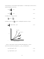
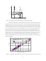
shows the calibration of all three sensors at the two temperatures T∞,1 = 9.0°C, and T∞,2 = 14.3 °C. As expected,
self-heating is negligible and the sensor voltage is proportional to current when the current is low (less than 2 mA).
Linear least squares curve fits are shown for each sensor, and the correlation coefficient is greater than 0.99 for all
but one sensor, indicating a strong linearity in the data.
3.6.3. Comparison of results
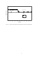
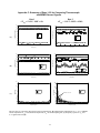
Sections 3.6.1 and 3.6.2 have outlined two independent calibration techniques for the MEMS sensors. As a
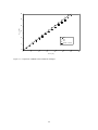
means of comparison, the reader is referred to Figure 3-7. In the figure, the calibration of each sensor is compared
using both the 4-wire resistance method and the in-situ method. A line representing T4-wire = Tin-situ is plotted. The
symbols on the graph indicate temperatures calculated using eq. (3.1) with the 4-wire resistance calibration data in
Table 3-2 , and using eq. (3.21) with the in-situ calibration data in Table 3-3. The graph indicates a good agreement
between the two calibrations in the temperature regions of interest to this study, specifically 0 to 15°C. This is in
part due to the fact that the calibration temperatures used in the in-situ method were 9.0 and 14.3°C. Extrapolation
of the resulting curve fits would naturally lead to higher deviations between the two calibration methods.
Table 3-3. Summary of MEMS serpentine resistance sensor by the in-situ method. (T∞,1 = 9.0°C, and T∞,2 =
14.3 C)
MEMS
sensor
Rs1
Rs2
Rs3
dV
m1 = 1
di s
[Ω]
i=0
dV2
m2 =
di s
111.3
28.6
5.18
113.9
29.2
5.30
22
[Ω]
Roα
[Ω/°C]
Co
[°C]
0.491
0.113
0.023
217.9
243.6
219.8
i=0
250
Sensor Voltage, Vs [mV]
200
Vs,1 = 0.1109 is
150
2
R = 0.999
100
Vs,2 = 0.0140 is
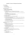
2
R = 0.997
50
0
-1000
-500
0
500
1000
1500
2000
2500
-50
Vs,3 = 0.0028 is
2
R = 0.885
-100
-150
Current, is [µA]
300
250
Sensor Voltage, Vs [mV]
Vs,1 = 0.1139 is
2
200
R =1
150
100
Vs,2 = 0.0292 i s
R2 = 1
50
0
-1000
-500
0
500
1000
1500
-50
2000
2500
Vs,3 = 0.0053 is
2
R =1
-100
-150
Current, is [µA]
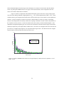
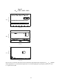
Figure 3-6 In-situ calibration of MEMS sensors at two temperatures, T∞,1 = 9.0°C (top), and T∞,2 = 14.3°C
(bottom)
23
30
25
Tin-situ (°C)
20
15
Ts1
10
Ts2
Ts3
T4-wire = Tin-situ
5
0
0
5
10
15
20
T4-wire (°C)
Figure 3-7. Comparison of MEMS sensor calibration techniques
24
25
30
35
Chapter 4: Experimental Procedures
4.1. Experimental Scope
This chapter will familiarize the reader with the procedures for each experiment and the methods used to
collect and process the data. The following list describes the objectives of each experiment.
1.
Methods of Calculating LMF – Develop a consistent method for quantifying the time averaged
liquid mass fraction (LMF) at the exit of a plate evaporator.
2.
Correlating Instrument Signals to LMF – Compare the signals of a thermocouple, MEMS thinfilm resistance sensor, and scattered laser light during the presence of small quantities of entrained
liquid droplets.
3.
Characterizing Exit Flows of Plate Evaporators – Measure the exit conditions of a 3-ton plate
evaporator at various superheats to demonstrate when and how liquid mass fraction (LMF) is
manifested at the evaporator exit.
4.
Comparing Thermocouples and MEMS Sensors – Investigate, using time-domain and frequencydomain analysis techniques, the feasibility of using either a thermocouple or the MEMS sensor to
detect and control LMF.
5.
MEMS Sensor Size vs. Sensitivity to LMF – Investigate how the surface area of a MEMS thin-film
resistance sensor affects its ability to detect LMF.
4.2. System Start-up and Operation
The reader is directed to Appendix B for the daily start-up procedures of system. These procedures were
followed until a stable operating point was reached close to the test conditions.
Operating the refrigeration loop was sometimes difficult, especially when using the thermostatic expansion
valve, because small perturbations of flowrates, or temperatures would take up to 30 minutes to return to steady
conditions. However, the expansion device (TXV or MXV) was typically set close to the desired superheat from the
previous days operation. When starting the system each day the inlet and outlet water temperatures were set first.
This was done by adjusting the hot water makeup flow from the condenser, and by adjusting the water flowrate with
the water pump bypass. Then the desired refrigerant setpoints were achieved by making incremental adjustments to
the refrigerant flowrate with the compressor bypass needle valves, or by adjusting the TXV superheat setpoint, or by
adjusting the evaporator load (water temperatures and flowrate). This was a delicate and time consuming process,
and often required several hours to reach the desired conditions.
During start-up it was important to monitor all of the flowrates, pressures, and temperatures on the data
acquisition monitor in order to avoid any problems. For example, the evaporator inlet water temperature could not
drop below 0°C, because the plate evaporator could have been seriously damaged if the water froze inside. Another
parameter that required special attention was the compressor suction temperature. There was no thermocouple in the
loop to monitor this temperature, so instead it was checked by hand to make sure the pipe was neither cold nor hot.
An adequate temperature was around room temperature. The compressor suction pipe was fed from the calorimeter
and the compressor bypass lines. The calorimeter heater power was adjusted so that all liquid droplets have been
evaporated, and the vapor stream to the compressor was around room temperature. Both of the needle valves on the
bypass lines were also adjusted to provide a mixed compressor suction stream at room temperature.
25
4.3. Procedures for Methods of Calculating LMF
4.3.1. Procedures and data collection
Two methods of calculating LMF were tested: 1) by an energy balance and 2) by direct flowrate
measurements. The two methods are compared in section 5.1 to determine which method most accurately measures
LMF. For this experiment the main and secondary evaporators were operating in parallel as shown in Figure 6-1.
The main evaporator was set to a high superheat temperature while the secondary evaporator injected a small
amount of saturated liquid into the test section. There were a total of 14 test runs for this experiment.
4.3.2. Test envelope
For this experiment the main evaporator superheat was held constant at ∆Tsup = 12°C. The main evaporator
flowrate was also held constant at mr = 40 g/s while the secondary evaporator flowrate m2 vaired from 0 to 1.5 g/s.
Data collection consisted of only low-speed sampling. A total of 150 data sets of the 20 instrument channels were
sampled and recorded for a total of 200 seconds.
Table 4-1. Test envelope for methods of calculating LMF
mr
m2
Te,in
40 g/s
0 to 1.5 g/s
∆Tsup
LMF
Tw,in and Tw,out
12°C
0 to 3.5%
2°C ±0.2°C
adjust to maintain ∆Tsup = 12°C
4.4. Procedures for Correlating Instrument Signals to LMF
4.4.1. Procedures and data collection
To correlate the thermocouple, MEMS sensor, and scattered light signals to the presence of droplets, a
known amount of liquid was injected into the test section. Both qualitative and quantitative comparisons of the
signals are made in section 5.2. The main evaporator was run at a high degree of superheat (12°C) to ensure that no
liquid was present at the evaporator exit, and a small amount of liquid was added to the test section using the
secondary evaporator. The same seven test section instruments listed in section 4.3 were again scanned at highspeeds. In addition, the largest MEMS sensor voltage, and the scattered laser light photodiode voltage were
measured using the lock-in amplifiers.
4.4.2. Test envelope
The test envelope for correlating the thermocouple, MEMS sensor, and scattered light signals to liquid
mass fraction is quite simple. The refrigeration system was run so that the main evaporator sustained a stable 12°C
superheat. This was done to ensure that the evaporator exit contained no liquid. The MEMS sensor current, is, was
set at 25 mA for the duration of the experiments. Lastly, the secondary evaporator was used to induce liquid into the
test section in the range of 0% < LMF < 4%. It will be shown in section 6.2 that liquid mass fractions greater than
4% are well into the unstable region of plate evaporator operation, and so they were not investigated.
26
4.5. Procedures for Characterizing Evaporator Exit Flows
4.5.1. Procedures and data collection
The goal of these experiments was to record the nature of multi-channel evaporator exit flows over a range
of superheats. For these experiments the system was configured for three different cases: 1) TXV control of the
main evaporator, 2) MXV control of the main evaporator, and 3) MXV control of the main and secondary
evaporators. In cases 1 and 2 there was no flow through the secondary evaporator. The refrigeration loop was run at
normal operating conditions (ie: high superheat), and then the evaporator superheat was decreased in each
successive run. The reduction of superheat was achieved by maintaining a constant inlet evaporator temperature,
Te,in, while at the same time lowering the water inlet temperature, Tw,in. The outlet evaporator temperature, Te,out, can
never be higher than the water inlet temperature because the evaporator is a counterflow heat exchanger. Therefore,
it is possible to control superheat by simultaneously raising or lowering the water inlet temperature, Tw,in, and by
adjusting the superheat setpoint of the TXV.
Data collection consisted of both low-speed sampling of all instrumentation, and high-speed sampling of
the test section instrumentation only. The low-speed data was used to measure system behavior over long periods of
time, and to calculate energy balances. The high-speed data was used to investigate the transient, non-equilibrium,
two-phase flow conditions at the evaporator exit. A total of 150 data sets of the 20 instrument channels were
sampled and recorded at low speeds for a total of 200 seconds. The HPVee data acquisition software determines the
low-speed data-sampling rate, which was a function of how many channels were multiplexed and how much data
was updated on the computer screen. HPVee could have been programmed to sample at a user-defined rate,
however that was not necessary for the slow data collection. The computer run time was recorded before each scan
so that the exact time between multiplexer scans was known. The majority of low-speed data collection was at an
average of 0.6 Hz.
High-speed sampling of the test section instrumentation was taken at a user-set 40 Hz. Seven channels were
sampled at this speed to measure
1.
Evaporator exit pressure,
2.
Static mixer exit pressure,
3.
Evaporator exit temperature,
4.
Temperature of thermocouple in glass tube,
5.
Vs1, the largest MEMS sensor voltage,
6.
Vs2, the middle MEMS sensor voltage, and
7.
Vs3, the smallest MEMS sensor voltage.
Each channel was scanned a total of 500 times, at 40 Hz, for a total of 12.5 seconds of data collection. The HP
multimeter was configured to advance on the external trigger connected to a wave generator putting out a square
wave TTL signal. The wave generator output frequency was dialed to exactly 40 Hz using a Fluke digital
multimeter. All high-speed data collection was performed immediately after the 3 minutes of low-speed data
collection. It can be reasonably assumed that process conditions did not vary significantly during the 60 seconds, or
so, it took to switch to high-speed data collection.
27
4.5.2. Test envelope
The test envelope for characterizing evaporator exit flows is shown in Table 4-2. For all cases the mass
flowrate, evaporator inlet temperature, and subcooled refrigerant temperature were held constant. Only the
superheat temperature, ∆Tsup, was varied from high to low superheat in order to describe how conditions at the
evaporator outlet become unstable.
Table 4-2. Test envelope for characterizing evaporator exit flows
mr
Te,in
40 g/s
∆Tsup
Tsub
12°C, 10°C, 8°C, ... unstable
Tw,in and Tw,out
is
2°C ±0.2°C
15°C ±0.5°C
adjust for desired evaporator load
25 mA
4.6. Procedures for Comparing Thermocouples and MEMS Sensors
4.6.1. Procedures and data collection
An important task of this project is to characterize the output signals of a beaded thermocouple and the
MEMS resistance sensors over a range of superheats and LMF. To accomplish this the main evaporator was
outfitted with the manual expansion valve described in section 2.2. The manual valve allows the main evaporator to
run at a fairly constant superheat, without the transients induced by a thermostatic expansion valve. The main
evaporator exit superheat was kept high (12°C) to ensure no entrained liquid was present. A small amount of liquid
was added to the test section inlet via the secondary evaporator, and the LMF was calculated using the procedure
outlined in section 5.2.
Data collection for these experiments consisted of both low-speed and high-speed data sampling. The same
20 channels measured in section 4.3 were again sampled at low frequency. The same holds true for the 7 channels
sampled at high frequency (40 Hz) for 12.5 seconds. During the high-speed data sampling, the MEMS sensor
current was set at 25 and 40 mA so that different heating values could be compared.
4.6.2. Test envelope
The test envelope for these experiments is outlined in Table 4-3. Notice that the conditions are very similar
to those in Table 4-2, and for good reason. It is important to investigate the behavior of the thermocouple and
MEMS sensors over know liquid fractions and superheat conditions would be expected in a real system with TXV
control. The superheat was varied from 12°C to 8°C. Anything lower than 8°C superheat caused the main
evaporator to spill liquid into the test section which would have biased our measurements of liquid mass fraction.
Table 4-3. Test envelope for comparing thermocouples and MEMS sensors
mr
Te,in
40 g/s
∆Tsup
LMF
Tw,in and Tw,out
is
12°C, 10°C, 8°C
0 to 2%
adjust for desired evaporator load
25 and 40 mA
2°C ±0.2°C
28
Chapter 5: Experimental Results
5.1. Methods of Calculating LMF
Maldistribution in plate evaporators is evident when liquid droplets are entrained in the superheated vapor
stream exiting the evaporator. One objective of this work is to develop a consistent method for measuring the liquid
mass fraction (LMF) of entrained liquid. Two methods for measuring LMF are compared, they are: 1) energy
balance method, and 2) direct measurement method. The energy balance method is based on the reduction of vapor
temperature at the static mixer due to the evaporation of droplets. The direct measurement method calculates LMF
by independently measuring the mass flowrate of superheated vapor and entrained liquid droplets.
LMF is defined here as the ratio of the mass flow rate of entrained liquid and the total mass flow rate. LMF
should not be confused with quality, which describes vapor that is saturated. Assuming liquid droplets and vapor
have the same velocity at a given pipe cross-section LMF can be formulated as
LMF [%] =
& liquid
m
& liquid + m
& vapor
m
× 100
(5.1)
Figure 5-1 shows a schematic of the main evaporator, secondary evaporator, test section with the static
mixer, and associated instrumentation. Stream 1 is superheated vapor exiting the main evaporator with a mass
flowrate m
& r , temperature Te,out, and pressure Pe. For all test conditions the main evaporator was run with 12°C
superheat, so it can be assumed with good accuracy that stream 1 is comprised solely of superheated vapor. Stream
2, on the other hand, is a low quality mixture at pressure Pe with mass flow rate
& 2 . The two streams mix in the
m
static mixer and exit as a single-phase superheated vapor at temperature Tmix. It is assumed that heat loss to the
environment is negligible and that all liquid droplets are evaporated before exiting the static mixer.
For the direct measurement method the definition of LMF, eq. (5.1), must be modified to give the LMF
directly from knowledge of the flow rates m
& r and
LMF [ % ] =
& 2 , and stream 2 inlet quality.
m
& 2 (1 − x 2 )
m
× 100
& r +m
&2
m
(5.2)
29
MEMS
Sensor
Pevap Tr,out
5
4
Stream 1
Pmix Tmix
Tr,glass
x2
Main
Evaporator
Stream 2
Secondary
Evaporator
Static Mixer
6
glass tube
Expansion Valve
3
T2,sub
water
mr
Main
Flowmeter
Secondary
Flowmeter
m2
1
Figure 5-1. Schematic of evaporators, static mixer, and test section instrumentation used to determine LMF
Both mass flow rates are measured by the Micro Motion flowmeters. However, the quality x2 must be determined
from the subcooled liquid temperature before expansion T2,sub (state 1 in Figure 5-2), and the pressure at the exit of
the secondary evaporator Pe. It is assumed that stream 2 undergoes a constant enthalpy expansion from T2,sub to a
low quality mixture at the exit pressure Pe. The quality x2 is thereby determined by Pe and the enthalpy of the
subcooled liquid before expansion. Figure 5-2 outlines this process on a P-h diagram.
The LMF entering the test section can also be calculated by the energy balance method. For this method it
is assumed that states 4 and 6 in Figure 5-2 are completely defined by the independent measurements of temperature
and pressure. Also, it is assumed that the two streams are completely mixed before exiting the static mixer with no
heat loss to the surroundings. State 2 is still at pressure Pe, but this time the quality is assumed to be unknown. An
energy balance of the adiabatic mixing of superheated vapor and unknown quality gives
& r ( h r − h mix ) = m
& 2 (1- x 2 )h fg + m
& 2 ( h mix − h sat )
m
(5.3)
The left hand side of the equation is the energy lost from the superheated vapor stream during the mixing process.
The right hand side accounts for the energy gained by the low-quality mixture of stream 2 during evaporation and
mixing. The first term is the heat of vaporization required to boil liquid droplets to the saturation temperature, and
the second term is the energy necessary to heat saturated vapor to the final state at the static mixer exit. The mass
flowrates
& r and m
& 2 are measured, and all of the enthalpies can be determined from pressure and temperature
m
measurements. The exit quality of the secondary evaporator can now be solved for directly. Once x2 is evaluated
using eq. (5.3) the LMF can be calculated using eq. (5.2).
30
T2,sub
P
1
Tr,out
3
5
2
Pevap
4
x2
Pmix
6
hsat hmix
h2
hr
h
Figure 5-2. P-h diagram of entrained liquid evaporating in a superheated vapor stream
A comparison of both methods of calculating LMF is shown in Figure 5-3. Both sets of data show a linear
relationship of LMF to
& 2 , the mass flow rate of stream 2. Error bars for each data point indicate the uncertainty
m
in LMF due to instrument errors only. The instrument error was calculated using the methods developed by Moffat
[6]. The true LMF at the inlet to the test section is most accurately represented by the direct measurement method of
eq. (5.2). This statement is based not just on the fact that the direct measurement method has less instrument error
(smaller error bars), but because the energy balance method is based upon several simplifying assumptions. First,
the energy balance method assumes no interaction between refrigerant and oil. The oil present in the suction line
(measured to be 0.2 to 0.3%) will absorb liquid droplets, thereby preventing them from evaporating [7]. This causes
a negative departure of the calculated LMF from the true LMF. Second, the energy balance method assumes
complete evaporation and mixing of the two streams before the static mixer outlet. Third, it assumes that the walls
of the mixer are adiabatic.
3.5
LMF by direct measurement
3.0
LMF by energy balance
Linear (LMF by energy balance)
Linear (LMF by direct measurement)
LMF [%]
2.5
2.0
1.5
1.0
0.5
0.0
0.0
0.2
0.4
0.6
0.8
1.0
1.2
1.4
1.6
Mass Flowrate of Stream 2 [g/sec]
Figure 5-3. Comparison of LMF calculated from (1) direct measurement method, and (2) energy balance method
31
Figure 5-3 also provides a calibration for estimating the systematic error in using the energy balance
method for determining the time-averaged liquid mass fraction. The LMF as a function of
& 2 for both methods
m
can be described by the following two linear relationships
LMFDIRECT = 2.145 m
&2
(5.4)
& 2 − 0186
LMFENERGY = 2.145 m
.
(5.5)
Writing these two equations in terms of
& 2 and setting them equal will give the following equation for the actual
m
LMF from the LMF determined by the energy balance method
LMF = LMFDIRECT =
LMFENERGY + 0.186
0.924
(5.6)
Eq. (5.6) will be used in section 5.3 to calculate the liquid mass fraction present at the evaporator outlet for the
characterizing evaporator exit flows experiment.
Now that the systematic error in the energy balance method for calculating LMF can be accounted for by
using eq. (5.6), it is possible to accurately measure the time averaged LMF present in a multi-channel evaporator
system. In section 5.2 the outlet conditions of a multi-channel evaporator fed by either a thermostatic expansion
valve, or a manual expansion valve, are studied. For these tests only the main evaporator in Figure 5-1 was used.
Consequently, we could only measure the total refrigerant mass flow rate
mass flow rate of liquid
& r , which in this case is equal to the
m
& liq plus the mass flow rate of superheated vapor m
& vapor at the evaporator outlet. The
m
total energy lost from the superheated vapor during evaporation of the entrained liquid in the static mixer is
& vapor ( h r − h mix )
Q evap = m
This is the same as the left hand side of eq. (5.3) with
(5.7)
& vapor . The enthalpy at the exit of the
& r replaced with m
m
static mixer hmix can easily be found from pressure and temperature measurements, but the superheated vapor
enthalpy hr is a little more complicated because the superheated vapor temperature could not be directly measured
by a thermocouple when liquid was present at the evaporator outlet. In order to measure the vapor temperature the
thermocouple was shielded from droplet impacts. The experimental technique used to measure the vapor
temperature is described in Appendix A. The energy lost by the vapor is equal to the energy gained by the liquid
during evaporation and mixing, and can be written as
& liq h fg + m
& liq ( h mix − h sat )
Q evap = m
(5.8)
Eq. (5.7) and eq. (5.8) can be combined to solve for the liquid mass flow rate
& liq , which can then be substituted
m
into eq. (5.1) to solve for LMF. Finally, this LMF is substituted into eq. (5.6), which corrects for the systematic
error in the energy balance method.
32
5.2. Correlating instrument signals to LMF
Experiments were performed to correlate the output signals of a beaded thermocouple, the MEMS
resistance sensors, and scattered laser light with the presence of liquid mass fraction. For these experiments, the
secondary evaporator was used to inject liquid into the test section while the main evaporator was running at high
superheat (∆Tsup = 11.9°C). These tests were conducted to ensure that temperature oscillations of the beaded
thermocouple and MEMS sensor were caused by LMF, as opposed to some other phenomenon like evaporator
pressure fluctuations.
14
0
Ts,1
Light
12
-0.01
10
-0.02
8
-0.03
6
-0.04
4
-0.05
2
-0.06
0
Scattered Light Photodiode Voltage
Temperature ºC
Te,out
-0.07
0
1
2
3
4
5
6
7
8
9
10
11
12
Time [sec]
Figure 5-4. Evaporator outlet thermocouple temperature Te,out, MEMS sensor temperature Ts,1, and scattered laser
light photodiode voltage in the presence of small quantities of liquid (LMF=0.41%)
For these tests, an exposed beaded thermocouple, the largest MEMS sensor R1, and the scattered laser light
signals were sampled at 40 Hz for 12.5 seconds. The thermocouple was located in the glass tube (see schematic in
Figure 5-1) such that the exposed bead was in the center of the pipe cross section. In this way, the thermocouple
could be impacted by entrained refrigerant droplets while measuring Te,out, the evaporator outlet temperature. Figure
5-4 shows the time traces of these three signals for very small amounts of liquid (LMF = 0.41%) with high
superheat, ∆Tsup = 11.9°C. The sensor was driven with a 25 mA DC current.
The scattered laser light signal is important, because it directly correlates with the quantity of droplets
present in the test section. The photodiode voltage signal decreases as more droplets are present to scatter the beam.
Notice that the signal amplitudes of both the thermocouple and the MEMS sensor relate to the scattered light (and
thus droplets). There is a slight time lag between the two temperatures and the laser signal of about 1 second. This
is because the laser gives an instantaneous measure of the liquid fraction, whereas the thermocouple and sensor have
thermal capacitance which delays their response to liquid. Additionally, the laser was located 6 inches upstream of
the MEMS sensor, and 14 inches upstream of the thermocouple, so a further time delay can be expected for droplets
to travel the distance between the laser and the other instruments.
33
The MEMS sensor and scattered light signals were also measured with lock-in amplifiers for liquid
fractions up to 4%. The lock-in output is based upon the autocorrelation of the input signal to a reference signal.
For the scattered light signal, the laser beam chopper frequency was used as the reference signal. The chopper
frequency was tuned to 40 Hz, so the lock-in output was proportional only to that portion of the photodiode signal
having components at 40 Hz. The MEMS sensor was driven by a square-wave current, also at 40 Hz, with a
maximum amplitude of 20 mA supplied by a wave generator. It is important to set the driving current frequency
much higher than the sensor time constant, so that the sensor “sees” the oscillating current as if it were constant.
Figure 5-5 shows these results. The lock-in output of each signal has been normalized their respective maximal
value (at the highest LMF). What this figure indicates quite clearly is the sensitivity of each instrument to the
amount of liquid in the test section. The scattered laser light is proportional to LMF, and is usable over a broad
range of LMF. The MEMS sensor, however, is extremely sensitive for liquid mass fractions less than 0.7%, and
then almost immediately becomes insensitive to additional liquid. The results are encouraging, because the high
sensitivity of the MEMS sensor to LMF below 0.7% indicates that the sensor could potentially be very useful in
detecting the onset of unstable superheat, such as in cases (1) and (2) in. In Figure 5-4, the smaller thermocouple
temperature fluctuations indicate that it is much less sensitive to low LMF than the MEMS sensor. An estimated
initial slope of the thermocouple response to LMF has been added to Figure 5-5, showing less sensitivity at low
LMF, but an increase in useable range. The MEMS sensor has an added degree of flexibility over a thermocouple,
because simply increasing the driving current can extend its useable range.
1.2
Initial slope indicates high sensitivity
Normalized Lock-in Output
1.0
Theoretical initial slope of
thermocouple.
(decreased sensitivity)
0.8
Scattered laser light sensitive over
a broad range of LMF
0.6
0.4
MEMS sensor
scattered laser light
0.2
0.0
0.0
1.0
2.0
3.0
4.0
Liquid Mass Fraction, LMF [%]
Figure 5-5. Normalized lock-in amplifier output of MEMS sensor and scattered laser light showing sensitivity to
droplets
5.3. Characterizing Evaporator Exit Flows
5.3.1. Introduction to experiments
One goal of this study was to characterize the exit conditions of a plate evaporator over a range of
superheat temperatures. Normal superheat temperatures are high enough to ensure that no liquid leaves the
34
evaporator. Reducing exit superheat too much can lead to maldistribution of the refrigerant amongst parallel
channels in the evaporator causing entrained liquid droplets to be present in the exit flow. This section describes the
results of a series of experiments that were conducted using a 3-ton capacity PHE as an evaporator. Three
configurations were tested: 1) PHE fed by a thermostatic expansion valve (TXV), 2) PHE fed by a manual
expansion valve (MXV), and 3) a two-evaporator arrangement in which LMF is manually controlled. Case (1) will
show the performance of a real evaporator/TXV system, case (2) eliminates the influence of TXV dynamics, and
case (3) allows for comparison of instrument signals under controlled LMF conditions.
The graphs in Figure 5-6, Figure 5-7, and Figure 5-8 are representative of the conditions witnessed at the
evaporator outlet for the three cases. The figures depict typical evaporator behavior, for each case, as the outlet
superheat temperature is reduced. For practical operation, it is always best to operate at the lowest possible
superheat that allows only vapor to exit the evaporator. There comes a point where further reductions in superheat,
for a given evaporator load, leads to incomplete evaporation within the channels, and entrained liquid appears at the
outlet. The liquid mass fraction (LMF) present during each test run, therefore, is a convenient basis for comparing
the three cases. Runs with relatively similar LMF, for each case, are grouped together in the figures. Initially, in
Figure 5-6, the superheat is relatively high, and not much liquid is present at the evaporator outlet. For the purpose
of comparison, this is what will be called low LMF. As superheat is reduced in Figure 5-7, and again in Figure 5-8,
the amount of entrained liquid increases. These two figures represent medium LMF, and high LMF, respectively.
Case (3) in Figure 5-6 represents the case of high superheat and almost no liquid at the exit. During this
test the main evaporator was operating with enough superheat, ∆Tsup = 8.6°C, to ensure that no liquid was present at
the outlet, and the secondary evaporator flow was shut off. As expected, the three thermocouples located in the test
section, Te,out, Tvapor, and Tmix, all indicate the same temperature. This is because there is no liquid present in the
exiting vapor stream. The MEMS sensor temperature, however, is more than 2°C higher than the surrounding
vapor. This makes sense since there are no droplets present. The heated sensor will always be hotter than the
surrounding vapor unless colder liquid droplets at the saturation temperature, Tsat, strike and cool the sensor.
5.3.2. Case (1) - TXV control of a plate evaporator
Case (1) in Figure 5-6, Figure 5-7, and Figure 5-8 shows the exit conditions of the main evaporator fed by a
pressure equalized TXV. In each figure the superheat is progressively reduced causing the LMF to increase.
Starting with Figure 5-6, the evaporator superheat is relatively stable at 8.9°C, but there is already an indication of
liquid at the outlet. Notice that there is a measurable difference between the vapor temperature, Tvapor, and the static
mixer outlet temperature, Tmix. Since the pressure drop in the mixer was negligible, this temperature difference can
only be explained by the evaporation of entrained liquid by the surrounding vapor within the mixer. Thus, the
magnitude of the temperature difference (Tvapor - Tmix) gives an indication of the relative amount of entrained liquid.
The thermocouple located directly at the evaporator outlet, Te,out, is also lower than the vapor temperature. This
thermocouple was suspended in the middle of the outlet pipe cross section, and could easily be impacted by any
liquid droplets that might be present in the flow stream. The fact that Te,out is lower than Tvapor is another indication
that liquid droplets were present during this run, because the droplets, at temperature Tsat, strike and cool the
thermocouple below the temperature of the surrounding vapor. In Figure 5-7 the superheat setpoint is reduced by
35
only a few tenths of a degree, but the measured LMF almost doubles, and the evaporator outlet temperature, Te,out,
begins to fluctuate by more than 2°C. This condition can be seen in Figure 5-7. Consider for a moment graph (a)
for this case, which shows the outlet temperatures during the entire test run. The Te,out temperature oscillations seem
to be superimposed over a longer time scale fluctuation on the order of 3 minutes. This slow periodic fluctuation
could be a consequence of the TXV responding to the high superheat in the outlet pipe by gradually opening, and
increasing the refrigerant flow to the evaporator. The difference between case (1) and case (2) in Figure 5-8
indicates the temperature sensing bulb strapped to the outside of the outlet pipe can not react fast enough to the
liquid rapidly emerging at the outlet, and the valve opening eventually decreases to reduce refrigerant flow to the
evaporator, and increase superheat.
It is interesting to examine the behavior of the evaporator outlet thermocouple temperature, Te,out, and the
MEMS sensor temperature, Ts,1, at high sampling rates. Graphs (b) show these temperatures sampled at 40 Hz.
These data were taken immediately after the slow speed data in graph (a) had been collected. At low LMF (Figure
5-6) Te,out and Ts,1 appear constant, but as LMF increases there appears to be a definite temperature oscillation with a
period nearly equal to 7 seconds. This is supported by graphs (a) and (b) at medium LMF (Figure 5-7), and high
LMF (Figure 5-8). The pattern of the MEMS sensor temperature is similar to a sawtooth curve. The sawtooth
pattern is a result of liquid impacting the sensor in bursts, or clouds. Initially, a quantity of liquid strikes and rapidly
cools the sensor. Then the internal heat generation of the sensor causes the temperature to rise slowly, until the next
burst of liquid appears 7 seconds later. This is, of course, an simplified view of the process. Any amount of liquid
occurring in between these droplet clouds will disturb the rise of the sensor temperature, and this can be seen in
graph (b) of Figure 5-8. Notice how the sawtooth pattern of Ts,1 is quite jagged, which is most likely due to smaller
bunches of droplets distributed between the larger clouds that come every 7 seconds. It is important to mention that
the temperature oscillations of both the thermocouple, Te,out, and the sensor, Ts,1, correlate identically to clouds of
liquid that were large enough to be seen by the naked eye through the glass tube in the test section.
5.3.3. Case (2) - MXV control of a plate evaporator
Case (2) is similar to case (1), except that this time a manual expansion valve was used instead of the TXV.
The results of case (2) are presented in Figure 5-6, Figure 5-7, and Figure 5-8 in order of increasing LMF. The
purpose of the manual expansion valve was to study the outlet conditions of a multi-channel evaporator as superheat
is reduced, without the effects of TXV valve dynamics. By using a MXV, any phenomena witnessed at the
evaporator outlet will only be a consequence of the physical mechanisms of evaporation among the parallel
channels. For all case (2) test runs the valve position was fixed, and the system was allowed to come to a pseudosteady condition. What this means is that the amplitude of the temperature oscillations of Te,out and Ts,1 remained
fairly constant, and Tvapor, Tmix, and Tsat remained constant over the entire run. The most important comparison
between the TXV and MXV runs is that the sawtooth pattern of the MEMS sensor temperature occurs in both cases.
Again, the period of these temperature oscillations is on the order of 7 seconds. It can be inferred from the MXV
runs that entrained liquid, probably resulting from maldistribution between evaporator channels, emerges at the
outlet piping in organized clouds every 7 seconds. This is a significant finding, because it indicates that mists of
entrained liquid droplets will appear at regular and predictable intervals as a result of maldistribution within a multi-
36
channel evaporator. Furthermore, it seems that this regular pattern remains constant even with increasing amounts
of maldistribution, or measured liquid mass fraction.
5.3.4. Case (3) – Controlled LMF with a two-evaporator arrangement
Case (3) in Figure 5-6, Figure 5-7, and Figure 5-8 show what can occur at the evaporator outlet when there
is maldistribution between two parallel channels. The two-evaporator arrangement, shown schematically in Figure
5-1, was adjusted such that the 3-ton main evaporator was running with high superheat at the outlet, to ensure no
droplets, and the smaller secondary evaporator added a low quality mixture into the test section. Manual expansion
valves that were left at a fixed position during the test runs fed both evaporators. This simulated a two-channel
evaporator in which maldistribution can be manually adjusted between the channels. It should be noted that the test
runs shown for case (3) in the figures were selected such that the average LMF, and superheat during the run closely
matched those of case (1) and (2) for comparison. Specifically, the low LMF data is from run 19, the medium LMF
data is from run 11, and the high LMF data is from run 20 in Appendix B.
The first thing to notice between cases (1), (2), and (3) is the similarity of the thermocouple time traces
sampled at low speed (0.5 Hz), shown in graphs (a) in the figures. As LMF increases, the magnitude of the
evaporator outlet temperature fluctuations, Te,out, continues to increase. In Figure 5-7 and Figure 5-8, these
fluctuations are about the same amplitude for the TXV control, MXV control, and controlled LMF tests. The time
scale of the Te,out temperature fluctuations also seems to be relatively constant between the three cases. There is one
noticeable difference between case (3), and the behavior of a real evaporator in cases (1) and (2). When LMF is
added via the secondary evaporator, the evaporator outlet temperature, Te,out, is as much as 2°C lower than was
measured during the TXV and MXV tests. One possible explanation for this might be that there was more entrained
liquid present during the case (3) tests, but examination of the high speed (40 Hz) data in graph (b) tells us
something different. Suppose that instead of the entrained liquid coming in discrete mists every 7 seconds, the
droplets are more evenly distributed. If this were true, the time trace of the MEMS sensor temperature, Ts,1, would
not appear as a regular sawtooth pattern, but would appear more random due to smaller droplet mists impinging on
the sensor more frequently. This is exactly what case (3) in Figure 5-7 and Figure 5-8 indicates. The sensor and the
exposed thermocouple are cooled more frequently by droplet mists, and are prevented from warming back up to the
superheated vapor temperature.
Also notice that the Te,out and Ts,1 temperature fluctuations, on a slower scale, directly correlate with the
saturation temperature fluctuations. It seems that there are higher frequency temperature oscillations, due to
frequent cooling by droplet mists, superimposed over a slower average temperature change related to the saturation
temperature. The frequency spectra in graphs (c) tell this story, perhaps a little more clearly. Consider the
frequency spectrum for the three cases in Figure 5-8. A large spike at 0.16 Hz in all three cases dominates the
thermocouple and MEMS sensor signals. In other words, the signals have a characteristic period of 6.25 seconds.
Recall that the temperature-time data indicated that temperature oscillations had a period of about 7 seconds, and
that these oscillations coincided with droplet clouds witnessed in the glass tube. The TXV control, and MXV
control cases only have significant frequencies below 2 Hz, but the thermocouple and MEMS sensor signals contain
higher frequencies during the controlled LMF tests. These frequencies above 2 Hz indicate that indeed the
37
distribution of droplets was more uniform in case (3) than in case (1) or (2), which are dominated by discrete droplet
clouds at 7 second intervals.
5.3.5. Performance of the MEMS sensor
Although the performance of the sensor will be discussed in greater detail in section 5.5 and 5.6, it is
interesting to notice in Figure 5-6, Figure 5-7, and Figure 5-8 that the MEMS sensor is consistently more sensitive to
LMF than the exposed beaded thermocouple. This is encouraging, because with a first prototype sensor we have a
working device that is simple, yet gives us enough information to measure LMF in a multi-channel evaporator.
38
Case (2) MXV Control
∆Tsup = 8.9°C; LMF = 0.08%
12
12
10
10
Tvapor
Tmix
Te,out
Tsat
6
4
12
10
8
Tvapor
Tmix
Te,out
Tsat
6
4
2
2
0
50
100
150
200
16
14
14
Ts,1
50
100
150
Te,out
0
Ts,1
Tvapor
Te,out
Tsat
Tvapor
6
10
8
Tvapor
Ts,1
Te,out
Tsat
Te,out
6
2
0
8
9
10
11
12
1
2
3
4
5
Time [sec]
6
7
8
9
10
11
12
0
1
2
3
Time [sec]
50
40
40
140
0
0
50
120
Tvapor
Te,out
Ts,1
Tsat
6
0
7
Tvapor
8
4
6
100
10
2
5
80
Te,out
12
4
4
60
14
Tvapor
2
3
40
16
Ts,1
4
2
20
Time [sec]
Temperature ºC
10
1
Tsat
4
200
12
Temperature ºC
Temperature ºC
39
12
0
Tmix
Time [sec]
16
Te,out
Tvapor
6
0
0
Time [sec]
8
Te,out; Tmix; Tvapor
8
2
0
0
(b)
Case (3) Simulated Maldistribution
∆Tsup = 8.6°C; LMF = 0%
Temperature [°C]
8
Temperature [°C]
(a)
Temperature [°C]
Case (1) TXV Control
∆Tsup = 8.9°C; LMF = 0.09%
4
5
6
7
8
9
10
11
12
Time [sec]
50
40
Maximum of Ts,1
Ts,1
20
Ts,1
30
20
Magnitude
Te,out
30
Magnitude
(c)
Magnitude
Te,out
Maximum of Te,out
10
10
0
5
10
Frequency [Hz]
15
20
Ts,1
20
10
0
0
Te,out
30
0
0
5
10
Frequency [Hz]
15
20
0
5
10
15
20
Frequency [Hz]
Figure 5-6. Evaporator outlet temperature signal comparison at low LMF during TXV control, MXV control, and simulated maldistribution (a) during the entire
run, (b) at 40Hz sampling rate, and (c) in the frequency domain
Case (2) MXV Control
∆Tsup = 7.7°C; LMF = 0.25%
14
12
12
10
10
8
Tvapor
Tmix
Te,out
Tsat
6
2
2
0
0
100
150
50
100
10
10
8
Tvapor
6
Te,out
Ts,1
0
4
5
6
7
20
40
60
8
9
10
11
12
Te,out
Tsat
6
8
6
4
Tsat
2
3
4
5
6
7
8
9
10
11
12
0
1
2
3
4
5
6
7
8
9
10
11
12
Time [sec]
200
Peak Ts,1 = 475
150
Magnitude
150
Magnitude
Te,out
Ts,1
0
1
Peak Ts,1 = 370
Ts,1
Tvapor
2
200
100
140
10
Time [sec]
Te,out
120
12
8
Time [sec]
150
100
14
Tvapor
Ts,1
0
200
80
Time [sec]
0
3
4
0
2
2
Tvapor
Tmix
Te,out
Tsat
6
200
4
Tsat
2
Magnitude
150
Temperature ºC
12
12
Temperature ºC
Temperature ºC
40
14
1
8
Time [sec]
14
0
10
0
0
200
4
(c)
12
2
Time [sec]
(b)
Tvapor
Tsat
6
4
50
14
Te,out
Tmix
8
4
0
Case (3) Simulated Maldistribution
∆Tsup = 10.1°C; LMF = 0.28%
Temperature [°C]
14
Temperature [°C]
(a)
Temperature [°C]
Case (1) TXV Control
∆Tsup = 8.3°C; LMF = 0.14%
100
Te,out
Ts,1
Te,out
Ts,1
100
Maximum of Te,out
50
50
0
50
0
0
5
10
Frequency [Hz]
15
20
0
0
5
10
Frequency [Hz]
15
20
0
5
10
15
20
Frequency [Hz]
Figure 5-7. Evaporator outlet temperature signal comparison at medium LMF during TXV control, MXV control, and simulated maldistribution (a) during the
entire run, (b) at 40Hz sampling rate, and (c) in the frequency domain
Case (1) TXV Control
∆Tsup = 8.0°C; LMF = 0.38%
Case (2) MXV Control
∆Tsup = 7.2°C; LMF = 0.32%
12
12
10
10
Case (3) Simulated Maldistribution
∆Tsup = 8.6°C; LMF = 0.58%
10
8
Tvapor
Tmix
Te,out
Tsat
6
4
8
6
Tsat
Tvapor
4
0
50
100
150
50
100
10
8
8
6
4
Tvapor
Te,out
Ts,1
Tsat
0
200
0
5
6
7
8
9
10
11
6
4
Tvapor
Ts,1
Te,out
Tsat
80
100
120
140
8
6
Tvapor
Ts,1
9
11
Te,out
Tsat
2
0
1
2
3
4
5
6
7
8
10
12
0
1
2
3
4
5
Time [sec]
6
7
8
9
10
11
12
Time [sec]
200
200
Maximum Ts,1 = 470
Peak Ts,1 = 540
Magnitude
150
Te,out
100
Ts,1
50
150
100
Magnitude
Peak Ts,1 = 476
Te,out
Ts,1
50
0
10
Frequency [Hz]
15
20
Te,out
Ts,1
100
Maximum of Te,out
50
0
5
60
10
0
12
200
0
40
12
Time [sec]
150
20
14
0
4
Tmix
Tsat
Time [sec]
2
3
Tvapor
Te,out
4
2
Magnitude
150
Temperature ºC
10
Temperature ºC
Temperature ºC
41
12
2
4
Time [sec]
12
1
6
0
0
200
Time [sec]
0
8
2
0
0
(c)
Te,out
Tmix
2
2
(b)
Temperature [°C]
Temperature [°C]
(a)
Temperature [°C]
12
0
0
5
10
Frequency [Hz]
15
20
0
5
10
15
Frequency [Hz]
Figure 5-8. Evaporator outlet temperature signal comparison at high LMF during TXV control, MXV control, and simulated maldistribution (a) during the
entire run, (b) at 40Hz sampling rate, and (c) in the frequency domain
20
5.4. Comparison of thermocouple and MEMS sensor signals
5.4.1. Introduction to experiments
The response of a beaded thermocouple and three MEMS sensors were formally compared in the time and
frequency domains, at various superheats and LMF, in order to determine their potential feasibility for controlling
plate evaporators. These tests were conducted using the secondary evaporator to inject controlled amounts of LMF
into the test section. The main evaporator was operated in the superheated range with a mass flow rate of 40 g/s
nominally. In total, 25 separate runs were conducted over 3 different superheats (12°C, 10°C, and 8.5°C), and LMF
from 0 to 3.5%. A summary of each run, including time histories and frequency spectra of test section temperatures
can be found in Appendix B. Data collected during each run consisted of
1.
Global system parameters
These measurements included flow rates, pressures, and temperatures necessary for energy
balance calculations. The data was collected at 0.5 Hz for 200 seconds.
2.
Fast sampling of test section instrumentation
The raw scattered light photodiode voltage, evaporator pressure, MEMS sensor voltages, and all
test section thermocouples were recorded at 40 Hz for 12.5 seconds.
A sampling frequency of 40 Hz was selected because it provided the best opportunity to capture all
significant frequencies present in the thermocouple, MEMS sensor, and scattered light signals. During the facility
shake-down process, Fourier analysis of the raw output of each instrument (thermocouple, MEMS sensors, and
scattered light) revealed that any frequencies above 10 Hz did not make a significant contribution to the frequency
spectra. Therefore, the sampling rate was selected as close as possible to the maximum expected frequency, while
still being above twice the Nyquist frequency. The Fourier analysis was performed on a 4-channel digital
oscilloscope capable of detecting frequencies to the GHz range.
The graphs in Figure 5-9 highlight the behavior of the test section temperatures, over three different
superheats, as LMF was incresed. These graphs show the superheat temperature (∆Tsup = Tvapor - Tsat), the
temperature of the thermocouple located in the glass tube, Te,out, and the largest sensor temperature, Ts,1, all as a
function of LMF. A nice feature of the graphs is that they clearly indicate the sensitivity of the thermocouple and
MEMS sensor to increasing amounts of liquid. The bars on the thermocouple and sensor temperatures indicate the
range of temperatures measured during the entire 12.5 seconds of data collection time. The larger the error bars, the
more sensitive the instrument is to the presence of liquid droplets. In all three graphs the MEMS sensor is most
sensitive at LMF’s below 1%, which is exactly what the lock-in data (see section 5.2) revealed during the early
stages of experimentation. The thermocouple, however, is sensitive at higher LMF around 1.25%.
42
16
14
Tvapor
Tmix
Ts,1
Te,out
(a)
T - Tsat (C)
12
10
8
6
4
2
0
0
0.5
1
1.5
2
2.5
3
3.5
LMF (%)
14
14
12
Tvapor
Tmix
Ts,1
Te,out
12
Tmix
Ts,1
Te,out
10
T - Tsat (C)
10
T - Tsat (C)
Tvapor
8
6
8
6
4
4
2
2
0
0
0
0.5
1
1.5
2
2.5
3
3.5
0.0
0.5
1.0
1.5
2.0
2.5
LMF (%)
LMF (%)
(b)
(c)
Figure 5-9. (T - Tsat) vs. liquid mass fraction behavior of thermocouples (Tmix, Te,out, Tvapor), and MEMS sensor
temperature (Ts,1) at three superheats 12°C (a), 10°C (b), and 8.6°C (c)
Another interesting feature of the graphs is that the heated sensor temperature is often lower than the
thermocouple. At first this seems counterintuitive. One would think that a heated resistor would always be hotter
than a thermocouple simply because the self-heating would promote evaporation of liquid droplets. A possible
explanation for the lower sensor temperature could be that the sensor surface was covered completely by a thin film
of liquid (or possibly oil). If this were the case, then the thin liquid film would boil on the surface of the sensor.
The sensor temperature would be driven down very close to the saturation temperature of the liquid, because only a
slight excess temperature is required for boiling. In all three graphs, the excess sensor temperature rapidly
approaches Ts,1 - Tsat = 2°C. In addition, the surface area to mass ratio of the sensor is much larger than the
thermocouple, so a droplet has a greater cooling effect on the MEMS sensor than the thermocouple. Therefore, the
sensor temperature is lower than the thermocouple when sufficient droplets are present.
5.4.2. Time domain analysis
Other comparisons between the beaded thermocouple and the MEMS sensors can be made from Figure 510. This figure shows the thermocouple temperature, MEMS sensor temperature (for the largest sensor, R1),
saturation temperature, and scattered laser light photodiode voltage in the time domain at low liquid mass fraction
(LMF = 0.28%), and high liquid mass fraction (LMF = 1.76%). At low LMF, the MEMS sensor is most sensitive to
the presence of droplets. This is evident by the large amplitude temperature fluctuations of the sensor, compared to
43
relatively little temperature fluctuation by the thermocouple. When large amounts of liquid are present the MEMS
sensor is unable to detect the increasing amount of liquid, but the thermocouple now is becoming more sensitive to
liquid. At the higher LMF, the temperature fluctuations of the thermocouple increase, and those of the MEMS
sensor decrease.
It is important to notice that there are both slow and fast frequency components in the thermocouple and the
MEMS sensor temperature traces. The slow frequency component in both temperatures is exactly in phase with the
saturation temperature displayed on the bottom of the figures. Saturation temperature varies with evaporation
pressure, which oscillates due to the nature of the two-phase evaporating flow in the evaporator. Superimposed on
top of the slow fluctuation is the high frequency content. It is the high frequency oscillation that is a result of
droplets impinging on the surface of the sensor (and thermocouple).
The trace of the scattered laser light photodiode voltage in both figures gives a relative indication of the
amount of liquid present during the run. When LMF is only 0.28%, the scattered light signal amplitude fluctuation
is about 0.01 Volts, but when LMF = 1.76%, amplitude variation is slightly higher. There are also several large
amplitude spikes on the order of 0.5 Volts. These larger spikes are related to large clouds of droplets that were
visually observed through the glass tube mounted in the test section. Notice that during high LMF the thermocouple
temperature drops rapidly after the passage of a droplet cloud, but the MEMS sensor is unable to respond to the
additional liquid.
LMF = 0.28%
LMF = 1.76%
-0.05
(a)
Temperature ºC
10
8
-0.1
6
4
Te,out
Tsat
Ts,1
Light
-0.15
2
0
1
2
3
4
5
6
7
8
9
10
11
Light
-0.1
6
4
-0.15
2
0
-0.2
0
12
1
2
3
4
5
6
7
8
9
10
11
12
Time [sec]
120
120
Magnitude
160
Magnitude
Tsat
8
160
Te,out
Ts,1
80
Ts,1
-0.05
Time [sec]
(b)
Te,out
10
-0.2
0
0
12
Temperature ºC
12
Scattered Light Photodiode Voltage
14
Scattered Light Photodiode Voltage
0
14
Maximum of Te,out
40
Te,out
Ts,1
80
40
0
0
0
5
10
15
20
0
Frequency [Hz]
5
10
15
20
Frequency [Hz]
Figure 5-10 Thermocouple (Te,out), MEMS sensor (Ts,1), and scattered laser light signals in the time domain (a),
and frequency domain (b), for LMF = 0.28% (left), and LMF = 1.76% (right)
44
5.4.3. Frequency domain analysis
Additional information about the performance of the thermocouple and MEMS sensor can be obtained by
examining the frequency content of the signals. The power spectra of both signals is shown in graphs (b) Figure 510 for both low and high LMF. Fast Fourier Transform analysis was performed on the discrete temperature signals
using the HP-VEE software, by first subtracting the mean of each signal from the original data set. This was done
to remove the DC component of the each signal, thereby leaving only the oscillating portion of the temperature
caused by both impingement of liquid droplets, and saturation temperature fluctuation. The first large spike at 0.16
Hz in both figures is due to the saturation temperature fluctuation. All of the other frequencies can be attributed to
the presence of liquid droplets. In both figures, the significant frequencies die out around 5 Hz. Initially, it was
thought that the MEMS sensor would be able to detect individual droplet impacts at frequencies above 100 Hz. This
is clearly not the case, especially at the higher LMF’s when droplet clouds are observed visually in the glass tube.
1.5
1.5
1.0
1.0
Magnitude
Magnitude
peaks at 0.25 Hz and 1 Hz
peak at 0.8 Hz
0.5
0.5
0.0
0.0
0
5
10
Frequency [Hz]
15
20
0
(a)
5
10
Frequency [Hz]
15
20
(b)
Figure 5-11. Frequency spectra of the scattered laser light signal at low LMF (a), and high LMF (b). (low
LMF = 0.28%, high LMF = 1.76%)
Even the scattered laser light can not detect the passing of individual droplets. The power spectra of the
scattered laser light photodiode voltage are shown in Figure 5-11, for LMF = 0.28% and 1.76%. At higher LMF
there is clearly a stronger signal, indicating more scattering due to liquid droplets. There are more sophisticated
techniques for measuring droplet size, velocity, and distribution, such as phase/Doppler particle analysis (P/DPA)
and laser-Doppler velocimetry (LDV). These laser diagnostics techniques have seen widespread use in combustion
research and aerosol sprays. They require very expensive laser equipment that is extremely difficult to calibrate,
which is why those techniques were not used in this investigation.
5.4.4. Effect of MEMS sensor surface area on sensitivity to droplets
Entrained liquid droplets smaller than 50 µm in diameter traveling at 10 m/s have been measured in
horizontal tube evaporators [2]. It was suspected that the size of the sensor would directly affect its ability to detect
such small droplets in the flow stream. For example, if a droplet is large enough to completely coat the small sensor
upon impact, it is sure to drop the sensor temperature very close to the liquid temperature. However, the same
droplet impacting the large sensor would only cover about 7% of the total surface area, and could not bring possibly
lower the sensor temperature completely to the liquid temperature. If the sensors are indeed sensitive enough to be
45
affected individual droplets, then the larger sensor should prove less sensitive at lower LMF’s than the smallest
sensor. By placing three MEMS sensors of varying size on the same substrate, a direct comparison of the size
effects can be made at identical flow conditions.
Figure 5-12 shows a comparison of the normalized frequency spectra of the time-varying voltage signal
from each sensor during conditions of high superheat, ∆Tsup = 10°C, and low liquid fraction, LMF = 0.32%. These
conditions allow a good comparison between the three sensors because they are most sensitive at lower liquid mass
fractions. Clearly, the frequency content of each sensor is almost identical. In some ways this is encouraging
because it tells designers that an extremely small sensor requiring a minimum of current can detect the dynamics of
the evaporator exit flow, however, it casts some doubt on the sensor’s ability to detect individual droplets. If the
distribution of droplets through the pipe cross section can be assumed to be uniform, then the larger sensor should
naturally be impacted by more droplets than a smaller sensor. The sensors were designed to have the same heat flux
per unit area, so a higher impact frequency was expected from the largest sensor. The data does not show a higher
impact frequency associated with increased sensor surface area.
0.5
0.4
0.4
0.3
Magnitude
2
R1=107.03 Ω , A=1mm
2
R2=27.51 Ω , A=.25mm
0.3
2
R3=5.01 Ω , A=.063m m
0.2
0.2
0.1
0.1
0.0
0
2
4
6
8
10
12
14
16
18
20
Frequency [Hz]
Figure 5-12. Effect of MEMS sensor surface area on signal frequency content for run 10; superheat = 10.0°C;
LMF = 0.32%
46
Chapter 6: Conclusions and Recommendations
6.1. Conclusions
The outlet flow of a 15 kW plate evaporator fed by a TXV was studied over a range of superheats from
12°C to 7°C, in order to investigate how decreasing superheat affects droplet generation at the evaporator exit. It
was discovered that entrained refrigerant droplets appeared in the exiting superheated vapor stream at superheat
temperatures as high as 9°C. The liquid droplets seemed to come in discrete mists, or clouds, at regular intervals.
These droplet mists caused fluctuations in the thermocouple and MEMS sensor signals that resembled a sawtooth
pattern with a period of about 7 seconds. The presence of these droplet mists was also confirmed by measurements
of scattered laser light intensity, and by visual inspection through the glass tube in the test section.
Reducing superheat below 8°C caused the thermostatic expansion valve to go unstable, otherwise known as
hunting. At the onset of unstable operation, the time-averaged LMF of entrained refrigerant droplets was measured
to be 0.4%. Droplet mist generation still occurred every 7 seconds during TXV hunting, but the characteristic
sawtooth temperature signal was superimposed over a slower mean temperature fluctuation with a period of nearly 3
minutes.
We have successfully fabricated and tested a prototype MEMS thin-film resistance sensor that can detect
entrained liquid droplets in a superheated vapor stream. Performance of the sensor was investigated over a range of
liquid mass fraction up to 4%, and superheat temperatures from 8°C to 12°C. Data collected over these conditions
indicates that the sensor is best used when liquid fractions are below 1%. Greater amounts of liquid tend to saturate
the sensor, and prevent it from boiling off the excess liquid. The ability of the MEMS sensor to detect a small
entrained LMF was compared to that of an exposed beaded thermocouple, with encouraging results. Although the
thermocouple can indicate the presence of droplets over a wider range of LMF, the heated MEMS sensor has a much
greater sensitivity than the thermocouple. Experiments using a plate evaporator with TXV control revealed that by
the time TXV operation goes unstable, entrained liquid mass fractions are typically 0.4%. The sensor is most
sensitive from 0 to 1% LMF, and would therefore be a more attractive choice than a thermocouple for detecting
entrained liquid as superheat is reduced.
The case of maldistribution between two parallel evaporator channels was investigated to see if outlet
conditions would be similar to those seen in the 19 channel plate evaporator. A two-evaporator arrangement was
used to simulate having a plate evaporator with only two refrigerant passes. Maldistribution was created between
the two evaporators by running one evaporator (the 15 kW main evaporator) at high superheat, and running the other
(secondary evaporator) with quality at the outlet. These tests did not result in discrete droplet mist generation. The
droplet distribution appeared to be more uniform in time. This was reflected in both the temperature histories and
frequency spectra of the thermocouple and MEMS sensor signals. Picking a representative test run, say LMF =
0.58%, shows that there are significant frequencies in the MEMS sensor signal up to 6 Hz for the case of simulated
maldistribution, compared to significant frequencies only up to 2 Hz for the multi-channel evaporator with TXV
control. The higher frequencies experienced during simulated maldistribution tests is indicative of more frequent
47
droplet impacts on the sensor. The more frequently the sensor is impacted by droplets, then the more the droplet
mist will appear uniformly distributed in time.
Some remarks must also be made about the sensor design itself. Actually, three MEMS thin-film resistance
sensors of different size were made in the same silicon wafer. The sensors ranged from 0.0625 mm2 to 1 mm2 in
total surface area, and were designed to have equal heat flux. The best way to compare their performance is by their
frequency spectra. It has been shown that the frequency content of each sensor is nearly identical, indicating that
even the smallest sensor could be used to detect maldistribution in plate evaporators. This is especially encouraging
because it implies that a very small device could be manufactured, and even ganged together with several other
sensors, to measure the outlet conditions of each channel in a plate evaporator.
6.2. Recommendations
Probably the most successful outcome of this project is the production of a prototype MEMS thin-film
resistance sensor that can detect entrained liquid droplets in a superheated vapor stream. Results from this study
show that the sensor has the potential to detect the liquid mists entrained in the superheated vapor exiting plate
evaporators. A logical course of action would be to use the sensor to develop actuation and control strategies for
multi-valve operation. The experimental facility is already equipped with two parallel evaporators, and it would not
be too difficult to install normal scale expansion valves and actuators that can be linked through control circuitry to
the sensor. Although the ultimate goal of this project is to match newly developed MEMS sensors with
microfabricated valves, actuators, and control circuitry, it would first be useful to validate the concept of multi-valve
control with normal scale components. If multi-valve operation on a macro scale can control refrigerant distribution
in plate evaporators in a way that reduces superheat, which it surely can, then the focus should naturally shift
towards developing and incorporating microtechnology into refrigeration systems.
We recognize the fact that the simulated maldistribution tests employed two evaporators, which does not
exactly replicate the process of refrigerant distribution at the inlet of a real plate evaporator fed by a TXV. A more
realistic approach would be to use a single expansion valve and a plate evaporator with only 2 refrigerant channels.
Maldistribution could be induced in the evaporator by unevenly heating one side with an external tape heater.
However, the tests that were performed with the two-evaporator arrangement give some insight into the type of
outlet conditions that one could expect from a multi-channel evaporator operating with multi-valve control.
48
REFERENCES
[1] CRC Handbook of Chemistry and Physics, Cleveland, OH: CRC Press, 58th ed. (1977).
[2] Barnhart, J.S. and J.E. Peters, “An experimental investigation of flow patterns in a horizontal-tube evaporator,”
ACRC TR-28, Air Conditioning and Refrigeration Center, University of Illinois at Urbana-Champaign, (1992).
[3] Shannon, M.A., T.M. Leicht, P.S. Hrnjak, N.R. Miller, and F.A. Khan, “Thin-film resistance sensor for
measuring liquid mass fraction in super-heated refrigerant,” International Journal of Sensors and Actuators,
164-177, (2001).
[4] Hewlett-Packard Company, HP E1326B/E1411B 5 ½-Digit Multimeter User’s Manual, (1996).
[5] Bruun, H.H., Hot Wire Anemometry: Principles and Signal Analysis, Oxford: New York, (1995).
[6] Moffat, R.J., “Describing the uncertainties in experimental results,” Experimental Thermal and Fluid Science,
v.1, 3-17, (1988).
[7] Martz, W.L., C.M. Burton, and A.J. Jacobi, “Vapor-liquid equilibria for R-22, R-134a, R-125, and R-32/125
with a polyol ester lubricant: measurements and departure from ideality,” ASHRAE Transactions, v.102, 367374, (1996).
49
Appendix A. Calibrating the Thermocouple in the Glass Tube to Measure Vapor
Temperature
In order to calculate the liquid mass fraction present at the evaporator outlet using the energy balance
method described in section 5.1, it is necessary to know the vapor enthalpy, state 4 in Figure 5.2. The vapor
enthalpy is found using thermodynamic property relations with the evaporator outlet pressure and the vapor
temperature. In a real system, refrigerant side maldistribution results in a non-equilibrium mixture of entrained
liquid within a superheated vapor, making it difficult to determine the vapor temperature with a high degree of
certainty. A thermocouple inserted directly into the outlet pipe would be impacted by liquid droplets, causing the
thermocouple to indicate a temperature somewhere between the actual vapor temperature, Tvapor, and the liquid
saturation temperature. It was hypothesized that shielding the thermocouple from impacting droplets, while still
exposing it to the exiting vapor, could give a reasonably accurate measure of the superheated vapor temperature.
Referring to the schematic of the evaporators and test section, Figure 5.1, there are three thermocouples
downstream of the main evaporator. They are located at the main evaporator outlet, the glass tube, and the static
mixer outlet. The thermocouple in the glass tube was used to measure the actual vapor temperature, Tvapor, during
the test runs of case (1) and (2) in section 5.2. To do so, it was positioned such that the thermocouple bead was in
the recessed part of the glass tee, and out of direct contact from droplet impacts. Placing the thermocouple bead in
the relatively stagnant gas volume, instead of directly in the vapor flow, does introduce some error which was
calibrated in a simple experiment. In order to quantify this error, the system was run until a high degree of superheat
(∆Tsup = 10.5°C) remained stable with no indication of droplets. The thermocouple in the glass tee was initially
sheltered from the approaching vapor flow, and was then placed in the center of the pipe cross section in direct
contact with the approaching vapor flow. The temperature of the glass tube thermocouple, Tglass, and the static
mixer outlet thermocouple, Tmix, were recorded for 100 seconds while the glass thermocouple position was
adjusted, and the resulting time traces are shown in Figure A-1. The figure indicates that when the thermocouple is
sheltered from the approaching flow, Tglass will read 1.1°C higher than the true vapor temperature, Tmix, and when
the thermocouple is placed at the center of the pipe cross section, Tglass and Tmix are in agreement to within 0.1°C.
For all of the test conditions reported in section 5.2, the Tglass thermocouple was placed in the sheltered position so
that the vapor temperature could be measured, and the resulting temperature was corrected by 1.1°C to account for
the thermocouple position.
50
15
Temperature [°C]
14
∆Tavg = 0.1°C
∆Tavg = 1.1°C
13
12
Tglass
Tmix
11
10
0
10
20
30
40
50
60
70
80
90
100
Time [sec]
Figure A-1. Calibration of the thermocouple in the glass tube to measure vapor temperature
51
Appendix B. Procedures for Refrigeration System Startup
Power ON Sequence
1. turn on desktop PC
2. turn on HP Mainframe
3. turn on DC power supply
4. turn on power strip mounted on the wall
DAQ Software Instructions
1. run HP Vee from shortcut on the desktop
2. open file " C:\HP VeePrograms\JulyDAQ"
3. press the RUN arrow to begin data sampling
4. data collection procedures:
a) run Microsoft Excel and open file "C:\MSOffice\Templates\hpveetemplate"
b) enter number of data points desired in IF/THEN/ELSE box on the JulyDAQ screen (sampling rate is
about 1.5 Hz)
c) make sure the “To Excel” block will write the correct number of data points (ie: rows and columns) to the
Excel spreadsheet
d) click on Collect Data checkbox to begin data collection
e) DO NOT interrupt DAQ software during data collection!
f)
save the Excel worksheet under a new filename where ever you like
g) repeat (b) - (e) for new runs
5. High Speed data collection
a) connect the wave generator to the ext. trigger of the HP multimeter
b) set the wave generator to a square wave of magnitude 2.5V and adjust to the desired sampling frequency
c) open file “C:\HPVee Programs\FastDAQ”
d) press start button on the left hand side of the window to collect data; the multimeter block is set to sample
7 channels at 40Hz for 500 data points per channel; you may have to adjust the aperture time if you
choose another sampling frequency
e) save the data record under a new name
f)
press the start button on the right hand side of the screen to extract the data; this program will build the 7
arrays and also do a lot of post processing
g) return to “JulyDAQ” to monitor the system
Running Refrigeration Loop (refer to schematic)
1. Initial Startup
a) make sure the following valves are OPEN: ball valves at inlet & outlet to test section, manual TXV
(should still be set at last run condition)
b) run DAQ software (see above instructions)
c) plug water pump into power strip
d) OPEN both water line ball valves on the wall
e) OPEN flowmeter bypass ball valve located next to the flowmeter; this is necessary because the solenoid
valve sticks at startup so we have to bypass it
f)
turn ON compressor
g) CLOSE flowmeter bypass once system is stable
2. Operating Procedure
a) adjust desired flowrate using manual TXV (clockwise increases flowrate)
b) adjust water temperature using hot condenser water (gate valve very sensitive!)
c) use heater to keep suction line from frosting
3. Shutdown
a) turn OFF compressor
b) CLOSE test section ball valves
c) unplug water pump
d) CLOSE water line ball valves on the wall
52
Appendix C: Summary of Runs 1-25 for Comparing Thermocouple
and MEMS Sensor Signals
Run 1
∆Tsup = 12.0°C; LMF = 0%
Run 2
∆Tsup = 11.9°C; LMF = 0.28%
16
16
14
14
12
Temperature [°C]
(a)
Temperature [°C]
12
10
Tmix
Te,out
Tvapor
Tsat
8
6
10
8
Tvapor
Tmix
Te,out
Tsat
6
4
4
2
2
0
0
0
20
40
60
80
100
120
140
0
20
40
60
Time [sec]
80
100
120
Tvapor
Ts,1
Te,out
Tsat
140
Time [sec]
16
20
18
14
Te,out
Ts,1
16
Temperature ºC
(b)
Temperature ºC
12
14
Tvapor
12
10
Ts,1
Tvapor
Te,out
Tsat
8
6
10
8
6
4
4
2
2
0
0
0
1
2
3
4
5
6
7
8
9
10
11
12
0
1
2
3
4
Time [sec]
5
6
7
8
9
10
11
12
Time [sec]
50
160
40
30
Magnitude
(c)
Magnitude
120
Te,out
Ts,1
20
Te,out
Ts,1
80
Maximum of Te,out
40
10
0
0
0
5
10
15
20
Frequency [Hz]
0
5
10
15
20
Frequency [Hz]
(a) Time trace of evaporator outlet and test section temperatures; (b) Thermocouple temperatures (Te,out, Tvapor), MEMS
sensor temperature (Ts,1), and saturation temperature (Tsat) at 40 Hz sampling rate; (c) Frequency spectra of Ts,1 and
Te,out signals shown in (b)
53
Run 3
∆Tsup = 12.1°C; LMF = 0.39%
Run 4
∆Tsup = 12.0°C; LMF = 0.73%
16
16
14
14
12
Temperature [°C]
(a)
Temperature [°C]
12
10
8
Tvapor
Tmix
Te,out
Tsat
6
4
10
8
6
Tvapor
Te,out
4
2
2
0
0
0
20
40
60
80
100
120
0
140
20
40
60
16
Te,out
Tsat
140
Tvapor
Ts,1
12
Temperature ºC
Temperature ºC
120
160
14
Tvapor
Ts,1
12
10
8
6
Te,out
Tsat
10
8
6
4
4
2
2
0
0
0
1
2
3
4
5
6
7
8
9
10
11
12
0
1
2
3
4
Time [sec]
100
100
90
90
80
80
70
70
60
Te,out
50
Ts,1
Maximum of Te,out
40
5
6
7
8
9
10
11
12
Time [sec]
Magnitude
Magnitude
100
16
14
(c)
80
Time [sec]
Time [sec]
(b)
Tmix
Tsat
60
Ts,1
40
30
30
20
20
10
10
0
Te,out
Maximum of
Ts,1
50
0
0
5
10
15
20
Frequency [Hz]
0
5
10
15
20
Frequency [Hz]
(a) Time trace of evaporator outlet and test section temperatures; (b) Thermocouple temperatures (Te,out, Tvapor), MEMS
sensor temperature (Ts,1), and saturation temperature (Tsat) at 40 Hz sampling rate; (c) Frequency spectra of Ts,1 and
Te,out signals shown in (b)
54
Run 6
∆Tsup = 11.9°C; LMF = 1.30%
16
16
14
14
12
12
Temperature [°C]
(a)
Temperature [°C]
Run 5
∆Tsup = 12.0°C; LMF = 1.06%
10
8
6
4
Tvapor
Tmix
Te,out
Tsat
10
Tvapor
Te,out
8
6
4
2
2
0
0
0
20
40
60
80
100
120
140
0
20
40
60
Time [sec]
16
16
14
14
Te,out
Ts,1
Tsat
10
8
6
10
120
140
Tvapor
Ts,1
Te,out
Tsat
9
11
8
6
4
4
2
2
0
0
1
2
3
4
5
6
7
8
9
10
11
0
12
1
2
3
4
5
6
7
8
10
12
Time [sec]
Time [sec]
160
140
140
120
120
100
100
Magnitude
Magnitude
100
12
Temperature ºC
Temperature ºC
Tvapor
0
(c)
80
Time [sec]
12
(b)
Tmix
Tsat
Te,out
Ts,1
80
60
Te,out
80
Ts,1
60
40
40
20
20
0
0
0
5
10
15
20
0
5
10
15
20
Frequency [Hz]
Frequency [Hz]
(a) Time trace of evaporator outlet and test section temperatures; (b) Thermocouple temperatures (Te,out, Tvapor), MEMS
sensor temperature (Ts,1), and saturation temperature (Tsat) at 40 Hz sampling rate; (c) Frequency spectra of Ts,1 and
Te,out signals shown in (b)
55
Run 7
∆Tsup = 12.0°C; LMF = 0%
Run 8
∆Tsup = 11.9°C; LMF = 2.27%
16
16
14
14
(a)
Temperature [°C]
12
Tmix
Tsat
12
Temperature [°C]
Tvapor
Te,out
10
8
6
6
4
2
0
20
40
60
80
100
120
0
140
20
40
60
16
16
14
14
12
100
120
140
12
Tvapor
Te,out
Ts,1
Tsat
10
8
Temperature ºC
Temperature ºC
80
Time [sec]
Time [sec]
6
Tvapor
Te,out
Ts,1
Tsat
10
8
6
4
4
2
2
0
0
0
1
2
3
4
5
6
7
8
9
10
11
12
0
1
2
3
Time [sec]
160
80
120
60
Te,out
Ts,1
80
4
5
6
7
8
9
10
11
12
Time [sec]
Magnitude
Magnitude
Tsat
8
2
0
(c)
Tmix
Te,out
10
4
0
(b)
Tvapor
40
Te,out
Ts,1
40
20
0
0
0
5
10
15
20
Frequency [Hz]
0
5
10
15
20
Frequency [Hz]
(a) Time trace of evaporator outlet and test section temperatures; (b) Thermocouple temperatures (Te,out, Tvapor), MEMS
sensor temperature (Ts,1), and saturation temperature (Tsat) at 40 Hz sampling rate; (c) Frequency spectra of Ts,1 and
Te,out signals shown in (b)
56
Run 9
∆Tsup = 11.9°C; LMF = 3.06%
Run 10
∆Tsup = 10.2°C; LMF = 0%
16
14
14
12
Tvapor
Tmix
Te,out
Tsat
10
8
Temperature [°C]
(a)
Temperature [°C]
12
6
4
10
Tmix
Te,out
Tvapor
Tsat
8
6
4
2
2
0
0
0
20
40
60
80
100
120
140
0
20
40
60
80
Time [sec]
16
18
14
16
Temperature ºC
Temperature ºC
Te,out
10
Ts,1
Tsat
8
6
160
12
10
Te,out
Ts,1
Tvapor
Tsat
8
6
4
2
2
0
0
0
1
2
3
4
5
6
7
8
9
10
11
0
12
1
2
3
Time [sec]
50
50
40
40
30
4
5
6
7
8
9
10
11
12
Time [sec]
Magnitude
Magnitude
140
Tvapor
4
(c)
120
14
12
(b)
100
Time [sec]
Te,out
Ts,1
20
30
Te,out
Ts,1
20
10
10
0
0
0
5
10
15
0
20
5
10
15
20
Frequency [Hz]
Frequency [Hz]
(a) Time trace of evaporator outlet and test section temperatures; (b) Thermocouple temperatures (Te,out, Tvapor), MEMS
sensor temperature (Ts,1), and saturation temperature (Tsat) at 40 Hz sampling rate; (c) Frequency spectra of Ts,1 and
Te,out signals shown in (b)
57
Run 12
∆Tsup = 10.1°C; LMF = 0.45%
14
14
12
12
10
10
Temperature [°C]
(a)
Temperature [°C]
Run 11
∆Tsup = 10.1°C; LMF = 0.28%
8
Tvapor
Tmix
Te,out
Tsat
6
4
2
8
6
4
Tsat
0
0
20
40
60
80
100
120
140
0
20
40
60
80
Time [sec]
100
120
140
160
Time [sec]
14
14
12
12
10
10
Temperature ºC
Temperature ºC
Tmix
Te,out
2
0
(b)
Tvapor
8
6
4
Tvapor
Te,out
Ts,1
Tsat
Tvapor
Ts,1
Te,out
Tsat
9
11
8
6
4
2
2
0
0
0
1
2
3
4
5
6
7
8
9
10
11
0
12
1
2
3
4
5
6
7
8
10
12
Time [sec]
Time [sec]
100
100
Maximum Ts,1 = 142
80
Magnitude
(c)
Magnitude
80
Te,out
60
Ts,1
Maximum of Te,out
40
20
Te,out
Ts,1
60
40
20
0
0
0
5
10
15
20
0
Frequency [Hz]
5
10
15
20
Frequency [Hz]
(a) Time trace of evaporator outlet and test section temperatures; (b) Thermocouple temperatures (Te,out, Tvapor), MEMS
sensor temperature (Ts,1), and saturation temperature (Tsat) at 40 Hz sampling rate; (c) Frequency spectra of Ts,1 and
Te,out signals shown in (b)
58
Run 14
∆Tsup = 10.1°C; LMF = 1.07%
14
14
12
12
10
10
Temperature [°C]
(a)
Temperature [°C]
Run 13
∆Tsup = 10.0°C; LMF = 0.82%
8
6
Tvapor
Te,out
4
Tmix
Tsat
8
6
Tvapor
Te,out
4
Tmix
Tsat
2
2
0
0
0
20
40
60
80
100
120
140
160
0
20
40
60
Time [sec]
120
140
12
12
Tvapor
Te,out
Ts,1
Tsat
8
Tvapor
Te,out
Ts,1
Tsat
10
Temperature ºC
10
Temperature ºC
100
14
14
(b)
80
Time [sec]
6
8
6
4
4
2
2
0
0
0
1
2
3
4
5
6
7
8
9
10
11
12
0
1
2
3
4
Time [sec]
5
6
7
8
9
10
11
12
Time [sec]
120
120
110
100
100
90
80
Te,out
Ts,1
Maximum of Ts,1
70
60
Magnitude
(c)
Magnitude
80
50
40
Te,out
Ts,1
60
40
30
20
20
10
0
0
0
5
10
15
20
0
Frequency [Hz]
5
10
15
20
Frequency [Hz]
(a) Time trace of evaporator outlet and test section temperatures; (b) Thermocouple temperatures (Te,out, Tvapor), MEMS
sensor temperature (Ts,1), and saturation temperature (Tsat) at 40 Hz sampling rate; (c) Frequency spectra of Ts,1 and
Te,out signals shown in (b)
59
Run 15
∆Tsup = 10.2°C; LMF = 1.36%
Run 16
∆Tsup = 10.2°C; LMF = 1.78%
14
14
12
Tvapor
Te,out
10
Tmix
Tsat
Temperature [°C]
(a)
Temperature [°C]
12
8
6
4
2
10
Tvapor
Tmix
Te,out
Tsat
8
6
4
2
0
0
0
20
40
60
80
100
120
140
0
20
40
60
Time [sec]
80
100
120
140
Time [sec]
14
14
12
12
Tvapor
Te,out
Ts,1
Tsat
8
Tvapor
10
Temperature ºC
(b)
Temperature ºC
10
6
Te,out
8
Ts,1
Tsat
6
4
4
2
2
0
0
0
1
2
3
4
5
6
7
8
9
10
11
12
0
1
2
3
4
100
100
80
80
60
5
6
7
8
9
10
11
12
Time [sec]
Magnitude
(c)
Magnitude
Time [sec]
Te,out
Ts,1
40
20
Te,out
60
Ts,1
40
20
0
0
0
5
10
15
0
20
5
10
15
20
Frequency [Hz]
Frequency [Hz]
(a) Time trace of evaporator outlet and test section temperatures; (b) Thermocouple temperatures (Te,out, Tvapor), MEMS
sensor temperature (Ts,1), and saturation temperature (Tsat) at 40 Hz sampling rate; (c) Frequency spectra of Ts,1 and
Te,out signals shown in (b)
60
Run 17
∆Tsup = 10.1°C; LMF = 2.20%
Run 18
∆Tsup = 10.3°C; LMF = 3.07%
14
14
12
Tvapor
Tmix
Te,out
Tsat
10
8
Temperature [°C]
(a)
Temperature [°C]
12
6
4
10
Tvapor
Tmix
Te,out
Tsat
8
6
4
2
2
0
0
0
20
40
60
80
100
120
0
140
20
40
60
80
14
14
12
12
8
6
160
6
4
2
2
0
0
1
2
3
4
5
6
7
8
9
10
11
0
12
1
2
3
50
50
40
40
Magnitude
Te,out
30
4
5
6
7
8
9
10
11
12
Time [sec]
Time [sec]
Magnitude
140
Tvapor
Te,out
Ts,1
Tsat
8
4
0
(c)
120
10
Tvapor
Te,out
Ts,1
Tsat
Temperature ºC
Temperature ºC
10
(b)
100
Time [sec]
Time [sec]
Ts,1
20
10
Te,out
30
Ts,1
20
10
0
0
0
5
10
15
20
0
Frequency [Hz]
5
10
15
20
Frequency [Hz]
(a) Time trace of evaporator outlet and test section temperatures; (b) Thermocouple temperatures (Te,out, Tvapor), MEMS
sensor temperature (Ts,1), and saturation temperature (Tsat) at 40 Hz sampling rate; (c) Frequency spectra of Ts,1 and
Te,out signals shown in (b)
61
Run 19
∆Tsup = 8.6°C; LMF = 0%
Run 20
∆Tsup = 8.6°C; LMF = 0.58%
12
12
10
8
Temperature [°C]
(a)
Temperature [°C]
10
Tvapor
Tmix
6
Te,out
Tsat
4
2
8
6
Tvapor
Te,out
4
2
0
0
0
20
40
60
80
100
120
140
0
20
40
60
Time [sec]
140
12
10
Temperature ºC
Temperature ºC
120
Te,out
12
10
Tvapor
8
Tvapor
Te,out
Ts,1
Tsat
6
8
6
Tvapor
Ts,1
4
4
Te,out
Tsat
2
2
0
0
0
1
2
3
4
5
6
7
8
9
10
11
0
12
1
2
3
4
5
150
150
130
130
110
110
90
Magnitude
Te,out
Ts,1
70
50
90
10
10
10
8
9
10
11
12
15
20
Frequency [Hz]
Maximum Ts,1 = 470
Maximum of Te,out
Te,out
Ts,1
50
30
5
7
70
30
-10 0
6
Time [sec]
Time [sec]
Magnitude
100
14
14
(c)
80
Time [sec]
16
(b)
Tmix
Tsat
-10 0
5
10
15
20
Frequency [Hz]
(a) Time trace of evaporator outlet and test section temperatures; (b) Thermocouple temperatures (Te,out, Tvapor), MEMS
sensor temperature (Ts,1), and saturation temperature (Tsat) at 40 Hz sampling rate; (c) Frequency spectra of Ts,1 and
Te,out signals shown in (b)
62
Run 22
∆Tsup = 8.3°C; LMF = 1.04%
12
12
10
10
Tvapor
Te,out
8
Temperature [°C]
(a)
Temperature [°C]
Run 21
∆Tsup = 8.6°C; LMF = 0.71%
Tmix
Tsat
6
4
2
8
Tvapor
Te,out
6
4
2
0
0
0
20
40
60
80
100
120
140
0
20
40
60
Time [sec]
Tvapor
Te,out
Ts,1
Tsat
140
Tvapor
10
Temperature ºC
Temperature ºC
120
12
10
8
6
Te,out
Ts,1
8
Tsat
6
4
4
2
2
0
0
0
1
2
3
4
5
6
7
8
9
10
11
12
0
1
2
3
4
Time [sec]
5
6
7
8
9
10
11
12
Time [sec]
120
120
100
100
80
80
Te,out
Magnitude
Magnitude
100
14
12
(c)
80
Time [sec]
14
(b)
Tmix
Tsat
Ts,1
60
Maximum of Ts,1
40
Te,out
Ts,1
60
Maximum of Ts,1
40
20
20
0
0
0
5
10
15
20
0
Frequency [Hz]
5
10
15
20
Frequency [Hz]
(a) Time trace of evaporator outlet and test section temperatures; (b) Thermocouple temperatures (Te,out, Tvapor), MEMS
sensor temperature (Ts,1), and saturation temperature (Tsat) at 40 Hz sampling rate; (c) Frequency spectra of Ts,1 and
Te,out signals shown in (b)
63
Run 23
∆Tsup = 8.2°C; LMF = 1.27%
Run 24
∆Tsup = 8.4°C; LMF = 1.47%
12
12
Tvapor
Tsat
10
Te,out
Tmix
Temperature [°C]
(a)
Temperature [°C]
10
8
6
4
2
Tvapor
Tsat
6
4
2
0
0
0
20
40
60
80
100
120
140
0
20
40
60
14
140
Tvapor
Te,out
Ts,1
Tsat
10
Temperature ºC
Temperature ºC
120
12
Tvapor
Te,out
Ts,1
Tsat
10
8
6
8
6
4
4
2
2
0
0
0
1
2
3
4
5
6
7
8
9
10
11
12
0
1
2
3
4
Time [sec]
5
6
7
8
9
10
11
12
Time [sec]
200
200
180
180
160
160
140
140
Maximum of Te,out
120
Te,out
Magnitude
Magnitude
100
14
12
(c)
80
Time [sec]
Time [sec]
(b)
Te,out
Tmix
8
Ts,1
100
80
Ts,1
100
80
60
60
40
40
20
20
0
Te,out
120
0
0
5
10
15
20
0
Frequency [Hz]
5
10
15
20
Frequency [Hz]
(a) Time trace of evaporator outlet and test section temperatures; (b) Thermocouple temperatures (Te,out, Tvapor), MEMS
sensor temperature (Ts,1), and saturation temperature (Tsat) at 40 Hz sampling rate; (c) Frequency spectra of Ts,1 and
Te,out signals shown in (b)
64
Run 25
∆Tsup = 8.4°C; LMF = 2.03%
12
(a)
Temperature [°C]
10
Tvapor
Tsat
8
Te,out
Tmix
6
4
2
0
0
20
40
60
80
100
120
140
Time [sec]
14
12
Tvapor
Te,out
Ts,1
Tsat
(b)
Temperature ºC
10
8
6
4
2
0
0
1
2
3
4
5
6
7
8
9
10
11
12
Time [sec]
100
(c)
Magnitude
80
Te,out
60
Ts,1
40
20
0
0
5
10
15
20
Frequency [Hz]
(a) Time trace of evaporator outlet and test section temperatures; (b) Thermocouple temperatures (Te,out, Tvapor), MEMS
sensor temperature (Ts,1), and saturation temperature (Tsat) at 40 Hz sampling rate; (c) Frequency spectra of Ts,1 and
Te,out signals shown in (b)
65