Download Sin título

AN UHF FREQUENCY-MODULATED CONTINUOUS
WAVE WIND PROFILER - DEVELOPMENT AND
INITIAL RESULTS
A Thesis Presented
by
DAVID GARRIDO LOPEZ
Submitted to Universitat Politecnica de Catalunya
Escola Tecnica Superior d’Enginyeria de Telecomunicacio de Barcelona
in fulfillment of the requirements for the degree of
ENGINYERIA SUPERIOR DE TELECOMUNICACIO
January 2010
Electrical and Computer Engineering
AN UHF FREQUENCY-MODULATED CONTINUOUS
WAVE WIND PROFILER - DEVELOPMENT AND
INITIAL RESULTS
A Thesis Presented
by
DAVID GARRIDO LOPEZ
Approved as to style and content by:
Stephen J. Frasier, Professor
Electrical and Computer Engineering
To my mother and father for the struggles they have gone through in
their lives, and the support they have always given me.
ACKNOWLEDGMENTS
First of all I would like to thank Dr. Stephen Frasier for giving me the chance
to be here at MIRSL, and for all of the help he provided me. I have really learn a
lot from you. Being here at MIRSL has been an excellent experience that helped
me to improve my knowledge in some areas such as remote sensing, antennas, signal
processing or electronics. It also made me grow as an engineer, and experience other
ways of working and researching that I am sure will be useful in my future career.
Also I have to thank Jorge Salazar, Jorge Trabal and Rafael Medina, the support
and help they gave me. They were always willing to answer my questions, and that
was always very helpful. Ivona Kostadinova deserves a special consideration as well
because she introduced me to the radar and did the previous work with it which
helped me get to the point where I am now.
Finally, I want to thank my family for their support from a distance. Thanks to
them I did not feel alone, even with an ocean in between us.
iv
TABLE OF CONTENTS
Page
ACKNOWLEDGMENTS . . . . . . . . . . . . . . . . . . . . . . . . . . . . . . . . . . . . . . . . . . . . . iv
LIST OF TABLES . . . . . . . . . . . . . . . . . . . . . . . . . . . . . . . . . . . . . . . . . . . . . . . . . . . viii
LIST OF FIGURES . . . . . . . . . . . . . . . . . . . . . . . . . . . . . . . . . . . . . . . . . . . . . . . . . . . ix
CHAPTER
1. INTRODUCTION . . . . . . . . . . . . . . . . . . . . . . . . . . . . . . . . . . . . . . . . . . . . . . . . . 1
1.1
Motivation . . . . . . . . . . . . . . . . . . . . . . . . . . . . . . . . . . . . . . . . . . . . . . . . . . . . . . . 1
1.2
Summary of Chapters . . . . . . . . . . . . . . . . . . . . . . . . . . . . . . . . . . . . . . . . . . . . . 3
2. FMCW WIND PROFILER PRINCIPLES . . . . . . . . . . . . . . . . . . . . . . . . . 4
2.1
Atmospheric Boundary Layer . . . . . . . . . . . . . . . . . . . . . . . . . . . . . . . . . . . . . . 4
2.2
Clear Air Backscatter Theory . . . . . . . . . . . . . . . . . . . . . . . . . . . . . . . . . . . . . . 5
2.3
FMCW Radar Basics . . . . . . . . . . . . . . . . . . . . . . . . . . . . . . . . . . . . . . . . . . . . . 6
3. SYSTEM HARDWARE DESCRIPTION . . . . . . . . . . . . . . . . . . . . . . . . . . 9
3.1
3.2
System Overview . . . . . . . . . . . . . . . . . . . . . . . . . . . . . . . . . . . . . . . . . . . . . . . . . 9
3.1.1
Initial hardware configuration . . . . . . . . . . . . . . . . . . . . . . . . . . . . . . . . 9
3.1.2
FMCW Radar Previous Results . . . . . . . . . . . . . . . . . . . . . . . . . . . . . 13
3.1.3
FMCW Radar Current State . . . . . . . . . . . . . . . . . . . . . . . . . . . . . . . 18
Wind Profiler Subsystems . . . . . . . . . . . . . . . . . . . . . . . . . . . . . . . . . . . . . . . . 18
v
3.2.1
Control and Transmit Subsystem . . . . . . . . . . . . . . . . . . . . . . . . . . . . 19
3.2.2
Calibration Loop . . . . . . . . . . . . . . . . . . . . . . . . . . . . . . . . . . . . . . . . . . 21
3.2.3
Receiver Subsystem . . . . . . . . . . . . . . . . . . . . . . . . . . . . . . . . . . . . . . . 22
4. DATA ACQUISITION . . . . . . . . . . . . . . . . . . . . . . . . . . . . . . . . . . . . . . . . . . . . 25
4.1
24DSI6LN Data Acquisition Board . . . . . . . . . . . . . . . . . . . . . . . . . . . . . . . . . 26
4.2
Data Acquisition Program . . . . . . . . . . . . . . . . . . . . . . . . . . . . . . . . . . . . . . . . 27
4.3
Synchronization Program . . . . . . . . . . . . . . . . . . . . . . . . . . . . . . . . . . . . . . . . . 28
5. SIGNAL PROCESSING . . . . . . . . . . . . . . . . . . . . . . . . . . . . . . . . . . . . . . . . . . 30
5.1
Signal Processing Program . . . . . . . . . . . . . . . . . . . . . . . . . . . . . . . . . . . . . . . . 30
5.2
Noise Floor Estimation . . . . . . . . . . . . . . . . . . . . . . . . . . . . . . . . . . . . . . . . . . . 31
5.3
Minimum Detectable Signal . . . . . . . . . . . . . . . . . . . . . . . . . . . . . . . . . . . . . . . 32
6. ANTENNA ISOLATION . . . . . . . . . . . . . . . . . . . . . . . . . . . . . . . . . . . . . . . . . 35
6.1
Antenna Isolation Tests With New Shrouds . . . . . . . . . . . . . . . . . . . . . . . . . 36
7. GRAPHICAL USER INTERFACE . . . . . . . . . . . . . . . . . . . . . . . . . . . . . . . 39
8. CONCLUSIONS . . . . . . . . . . . . . . . . . . . . . . . . . . . . . . . . . . . . . . . . . . . . . . . . . . 41
8.1
Summary . . . . . . . . . . . . . . . . . . . . . . . . . . . . . . . . . . . . . . . . . . . . . . . . . . . . . . . 41
8.2
Future work . . . . . . . . . . . . . . . . . . . . . . . . . . . . . . . . . . . . . . . . . . . . . . . . . . . . 42
APPENDICES
A. DATA ACQUISITION PROGRAMS . . . . . . . . . . . . . . . . . . . . . . . . . . . . . . 43
A.1 main.c . . . . . . . . . . . . . . . . . . . . . . . . . . . . . . . . . . . . . . . . . . . . . . . . . . . . . . . . . 43
A.2 savedata.c . . . . . . . . . . . . . . . . . . . . . . . . . . . . . . . . . . . . . . . . . . . . . . . . . . . . . . 54
B. SYNCHRONIZATION PROGRAM . . . . . . . . . . . . . . . . . . . . . . . . . . . . . . . 69
B.1 pre processing david.pro . . . . . . . . . . . . . . . . . . . . . . . . . . . . . . . . . . . . . . . . . . 69
vi
C. SIGNAL PROCESSING PROGRAM . . . . . . . . . . . . . . . . . . . . . . . . . . . . . 74
C.1 windprof process david.pro . . . . . . . . . . . . . . . . . . . . . . . . . . . . . . . . . . . . . . . . 74
D. GRAPHICAL USER INTERFACE PROGRAM . . . . . . . . . . . . . . . . . . 80
D.1 wgui fmcw create.pro . . . . . . . . . . . . . . . . . . . . . . . . . . . . . . . . . . . . . . . . . . . . 80
D.2 wgui fmcw event.pro . . . . . . . . . . . . . . . . . . . . . . . . . . . . . . . . . . . . . . . . . . . . . 84
D.3 get conf file.pro . . . . . . . . . . . . . . . . . . . . . . . . . . . . . . . . . . . . . . . . . . . . . . . . . 86
D.4 run windprofiler.pro . . . . . . . . . . . . . . . . . . . . . . . . . . . . . . . . . . . . . . . . . . . . . . 88
D.5 reset.pro . . . . . . . . . . . . . . . . . . . . . . . . . . . . . . . . . . . . . . . . . . . . . . . . . . . . . . . 89
D.6 run daq.pro . . . . . . . . . . . . . . . . . . . . . . . . . . . . . . . . . . . . . . . . . . . . . . . . . . . . . 89
BIBLIOGRAPHY . . . . . . . . . . . . . . . . . . . . . . . . . . . . . . . . . . . . . . . . . . . . . . . . . . . 91
vii
LIST OF TABLES
Table
Page
3.1
Initial System specifications . . . . . . . . . . . . . . . . . . . . . . . . . . . . . . . . . . . . . . 10
3.2
Delay line specifications . . . . . . . . . . . . . . . . . . . . . . . . . . . . . . . . . . . . . . . . . . 22
viii
LIST OF FIGURES
Figure
Page
2.1
Boundary layer structure (from [6]) . . . . . . . . . . . . . . . . . . . . . . . . . . . . . . . . . 5
2.2
Time versus frequency diagram(a); FM signal (b). . . . . . . . . . . . . . . . . . . . . 7
2.3
Difference on instantaneous frequencies on FMCW . . . . . . . . . . . . . . . . . . . 8
3.1
Wind Profiler old configuration . . . . . . . . . . . . . . . . . . . . . . . . . . . . . . . . . . . 12
3.2
audio amplifier issue . . . . . . . . . . . . . . . . . . . . . . . . . . . . . . . . . . . . . . . . . . . . . 13
3.3
Shroud fence built around the Wind Profiler antennas . . . . . . . . . . . . . . . . 14
3.4
Antenna isolation and achieved transmit leakage cancellation . . . . . . . . . . 15
3.5
New FMCW Wind Profiler block diagram . . . . . . . . . . . . . . . . . . . . . . . . . . 17
3.6
Radar deployment in the laboratory . . . . . . . . . . . . . . . . . . . . . . . . . . . . . . . . 18
3.7
Altera Cyclone II EP2C20 FPGA . . . . . . . . . . . . . . . . . . . . . . . . . . . . . . . . . . 19
3.8
FPGA Control signals generation . . . . . . . . . . . . . . . . . . . . . . . . . . . . . . . . . . 20
3.9
Control and transmit subsystem box . . . . . . . . . . . . . . . . . . . . . . . . . . . . . . . 21
3.10 Receiver subsystem box . . . . . . . . . . . . . . . . . . . . . . . . . . . . . . . . . . . . . . . . . . 22
3.11 Audio module filter ringing . . . . . . . . . . . . . . . . . . . . . . . . . . . . . . . . . . . . . . . 24
4.1
24DSI6LN Data Acquisition Card . . . . . . . . . . . . . . . . . . . . . . . . . . . . . . . . . . 26
ix
5.1
Leakage and calibration signal processed . . . . . . . . . . . . . . . . . . . . . . . . . . . . 31
5.2
Noise floor estimation results . . . . . . . . . . . . . . . . . . . . . . . . . . . . . . . . . . . . . . 32
5.3
Noise floor estimation results with estimation of leakage method . . . . . . . 33
5.4
Minimum detectable signal plot . . . . . . . . . . . . . . . . . . . . . . . . . . . . . . . . . . . 34
5.5
Minimum detectable signal after subtraction of the noise floor . . . . . . . . . 34
6.1
Tilson Farm deployment point . . . . . . . . . . . . . . . . . . . . . . . . . . . . . . . . . . . . . 36
6.2
Received leakage without using shrouds . . . . . . . . . . . . . . . . . . . . . . . . . . . . . 37
6.3
Wind Profiler deployment with shrouds . . . . . . . . . . . . . . . . . . . . . . . . . . . . . 38
6.4
Received leakage using shrouds . . . . . . . . . . . . . . . . . . . . . . . . . . . . . . . . . . . . 38
7.1
Graphical User Interface . . . . . . . . . . . . . . . . . . . . . . . . . . . . . . . . . . . . . . . . . . 40
x
CHAPTER 1
INTRODUCTION
1.1
Motivation
The measurement of winds and processes taking place in the atmosphere is a fundamental requirement in both research and operational meteorology. This project is
focused on the processes taking place in the lower troposphere called the atmospheric
boundary layer (ABL). The ABL is important meteorologically in terms of assessing
of convective instability. The entrainment zone at the top of the ABL acts as a lid on
rising (and cooling) air parcels due to temperature inversion. An external mechanism
such as geographically forced uplift, vigorous surface heating or dry lines, can break
the entrainment layer, allowing the capped air parcels to rise freely. As a result,
vigorous convection will begin producing severe thunderstorms.
ABL research and studies help (i) develop and improve existing numerical weather
prediction models, (ii) understand the transfer of heat, water vapor and momentum
between the Earth and the atmosphere, (iii) refine the analytical description of turbulent processes and (iv) quantify the absorption and emission in the troposphere,
which is a major factor in shaping climate on Earth. The effect of the troposphere
on wave propagation has also been studied extensively for the purposes of improving
radio communications.
The main reason for FMCW radar development is the need for continuous monitoring of the winds and fields in the atmosphere, improving in-situ measurements.
Conventional radar profiler technologies are usually able to make atmospheric mea1
surements of the boundary layer, but preclude the lower part of the ABL, (around
150 meters). The Frequency Modulated Continuous Wave, Spaced Antenna (FMCWSA) Radar, that is being developed in University of Massachusetts - Amherst, at the
Microwave Sensing Laboratory (MIRSL), will allow measurements of the lower part
of the ABL.
The use of FMCW radars is introduced in order to improve the limitations of
pulsed radars. Pulsed radars are limited by the pulse-width and switching speed of the
transmit-receive switches because of the use of common antennas for both functions.
The pulsed nature of the radar dictates a higher transmitter power, and consequently
the need for switches that are both faster and high powered. FMCW radar alleviate
this problem by using separate antennas for transmit and receive, which also allows
use at short ranges. The problem in dual-antenna systems is parallax at low altitudes
due to the spatially separated antenna apertures, and some uncertainty in the actual
sampling volume.
The primary objective of this thesis is to explain the previous state of the radar,
providing a detailed account of it. Then to present the current state of the radar with
results and complete explanations to report conclusions.
2
1.2
Summary of Chapters
Chapter 2 gives a introduction to the atmospheric boundary layer, explains its
structure and characteristics followed by clear-air backscatter theory. After that the
principles of FMCW radars are explained. Chapter 3 presents an overview of the
FMCW Wind Profiler, and the initial configuration and previous results of the radar
are explained and commented.
Chapter 4 depicts the Wind Profiler data acquisition by presenting the Data Acquisition Card and programs. Chapter 5 explains the signal processing method used in
the Wind Profiler, and concludes by showing the radar’s minimum detectable signal.
In chapter 6 the new idea to improve the Wind Profiler antenna isolation is shown,
and the results obtained are provided. In chapter 7 the Graphical User Interface is
displayed. Finally, chapter 8 contains a brief summary of the research work presented
here, and conclusions and recommendations for future work are drawn.
3
CHAPTER 2
FMCW WIND PROFILER PRINCIPLES
2.1
Atmospheric Boundary Layer
The boundary layer is the lowest 1-2 km of the atmosphere, the region most
directly influenced by the exchange of momentum, heat, and water vapor at the
earth’s surface. Turbulent motions on time scales of an hour or less dominate the flow
in this region, transporting atmospheric properties both horizontally and vertically
through its depth. The mean properties of the flow in this layer, the wind speed,
temperature, and humidity experience their sharpest gradients in the first 50-100
m, appropriately called the surface layer. Turbulent exchange in this shallow layer
controls the exchange of heat, mass, and momentum at the surface and thereby the
state of the whole boundary layer. It is hardly surprising we should have a lively
curiosity about this region.
There are two main types of boundary layer. The convective boundary layer where
heat from the Earth’s surface creates positive buoyancy flux and instabilities that lead
to turbulences, and the stably stratified nocturnal boundary layer, where negative
buoyancy flux decreases the turbulences and stable stratified conditions prevail. The
ABL can reach over 3 km during daytime while the usual height at night is between
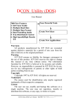
50 m. to 300 m. Typical boundary layer structure is depicted in Figure(2.1).
4
Figure 2.1: Boundary layer structure (from [6])
2.2
Clear Air Backscatter Theory
Backscattering occurs from refractive index irregularities in clear air and has a
relationship with the atmospheric structure and turbulence, as determined from experimental studies of angel echoes starting with Plank [1956] and Atlas [1959].
Radar backscattering from refractive index variation is able to provide helpful
information about the atmospheric structure. First radar outlines regions of increased
refractive index variability because of the enhanced backscattering. Second, the radar
backscatter contains quantitative information about the variability in the refractive
index field.
The radar backscattering from the clear air atmosphere, is caused by irregular
small-scale fluctuations in the radio refractive index produced by turbulent mixing
and is dependent on the atmospheric water vapor, temperature, and pressure. The
intensity of these fluctuations can be described by the structure constant Cn2 . In
1969 Ottersen [10] was the first to derive the relationship between the radar volume
5
reflectivity and refractive index structure as
1
η(λ) ≈ 0.38Cn2 λ− 3
(2.1)
For a given radar λ, the radar reflectivity η of a region of refractive index fluctuations is directly proportional to Cn2 when the length scale of one-half of the radar
wavelength falls within the inertial subrange. The more violent the turbulent mixing
the larger the displacements, and the stronger the inhomogeneities will be. So, strong
turbulence and sharp mean gradients contribute to high Cn2 values.
The radar backscatter can be originated by other sources such as Rayleigh scattering, for example from birds and insects, the size of which should be much smaller
than the radar wavelength and is proportional to λ−4 . In our application this kind of
scattering will be considered as undesired noise.
2.3
FMCW Radar Basics
FMCW is a common technique used on radars, that avoids the limitations of
pulsed radars. It consists on the transmission of a sinusoid whose frequency changes
over time, in our case linearly. Ideally the instantaneous frequency should augment
indefinitely with time, but in order to have a realistic system the frequency will
increase until a maximum value, and will start from the initial frequency once reached
that point. So, the instantaneous frequency will have a saw tooth shape as observed
in Figure(2.2).
The backscattered signal will be delayed by tdelay =
2R
,
c
where c is the speed of
light and R is the range to target as shown in Figure(2.3). It will be also attenuated
and possibly Doppler-shifted in case the target was not stationary. The received
signal will be then mixed with a replica of the transmitted signal, a sinusoidal signal
6
Figure 2.2: Time versus frequency diagram(a); FM signal (b).
for every target will be produced. The frequency of which is called beat frequency
and depends on the range to target and the radar parameters. For stationary targets,
the relation is as follows
R=
cTp
fb
2B
(2.2)
where R is the range to target, c is the speed of light, B is the chirp bandwidth and
Tp is the sweep time. Fast Fourier transform analysis is performed then in order to
convert frequency information to range. The range resolution of the system is
ΔR =
c
2B
(2.3)
Parameters such as B and Tp are configurable in an FMCW radar thus providing
flexibility to adapt to the most suitable mode, without change in the peak transmit
power for a given sensitivity.
7
Figure 2.3: Difference on instantaneous frequencies on FMCW
To retrieve velocities, it is possible to determine Doppler velocities comparing the
changes of phase of two consecutive pulses received. The maximum unambiguous
velocity that can be measured is determined by the radar operating frequency and
the pulse repetition frequency as
vrmax =
λ
fp
4
(2.4)
To maximize range resolution and sensitivity, both B and Tp should be as large as
possible. The value of Tp , however is constrained by the coherence time of the atmospheric echo because the presented theory is based on the assumption that the target
produces constant-frequency sinusoidal echo during the sweep [12]. The maximum
range for FMCW radars is determined by the sweep time Tp and the sampling frequency used in the A/D conversion. The latter gives us the maximum beat frequency
that can be detected without aliasing.
Rmax =
cTp
cTp fs
Fbmax =
2B
2B 2
8
(2.5)
CHAPTER 3
SYSTEM HARDWARE DESCRIPTION
3.1
System Overview
The current FMCW radar project started as an analog of the S-Band FMCW
boundary layer profiler developed in 2003 at University of Massachusetts at Amherst
[12]. The change from S-Band to UHF was proposed in order to reduce the Rayleigh
scattering from insects and birds which appeared to dominate the observed vertical
profile of the mean reflectivity at S-Band.
The current FMCW - Wind Profiler was started in the summer 2006 by the former
students Albert Genis during 2008 and Iva Kostadinova on 2008-2009. Many changes
have been introduced to the radar after upgrading and overcoming the different problems that were affecting the radar through several years.
The purpose of the next sections is to explain the latter hardware configuration
of the radar, and analyze the problems and changes that either were introduced or
are being introduced to solve them.
3.1.1
Initial hardware configuration
The FMCW wind profiler operates in the 900MHz ISM frequency band (902 - 928
MHz), with a center frequency of 915MHz. The chirp is generated by Direct Digital
Synthesizer (AD9858) with a bandwidth up to 25MHz and linear FM modulation. So
achieving a maximum range resolution of 6m.
9
Parameter
Transmitter
Center frequency
Peak Transmit power
Transmitter type
Sweep bandwidth
Sweep time
PRF
Antennas
Type
Gain
Polarization
Front to Back Ratio
Value
915MHz
30W
Solid State RF (SSRF)
≤25MHz
8.333ms
100Hz
Four Parabolic dish
18dB
Linear
22dB
Table 3.1: Initial System specifications
The default mode of operation had a PRF of 100Hz, and a duty cycle of 83.3%,
Tp = 8.33ms. These parameters allow detection of vertical unambiguous velocity up
to ±8.25m/s which exceeds the range of usual turbulent velocities on the boundary
layer (3-5m/s).
All the signals needed to start the radar, such as those used to start and set
up the DDS and synchronize and clock the sampling are generated by an FPGA
Cyclone II from Altera, designed by Iva Kostadinova and David Garrido Lopez. The
parameters of the radar such as bandwidth, PRF and Tp are configurable. This allows
for adaptation to the resolution and scenario as necessary. When (2.3), (2.4) and (2.5)
are taken into account it is possible to calculate the optimal configuration.
The transmit amplifier is a compact solid state RF power amplifier providing a
30W output. The antennas are 4’ diameter antenna parabolas, with dipole antenna
feeds, 19 degree beamwidth and 18dB of gain. The antennas have a broad beam, in
order to employ a spaced antenna technique for estimating horizontal winds. That
broad antenna beamwidth has its problems. The main problem associated with it
is inadequate isolation between transmitter and receiver. The transmitter leakage
10
received is powerful enough to saturate either the front-end of the receiver or the Data
Acquisition Board. To solve that problem an active cancellation loop was introduced,
using a vector modulator (AD8340) a replica of the leaked signal with opposite phase
is coupled to the receiver in order to cancel the leakage.
11
Figure 3.1: Wind Profiler old configuration
12
3.1.2
FMCW Radar Previous Results
After testing and deploying the FMCW radar, it turned out that there were some
noise and sensitivity problems in the previous design that needed to be fixed. In this
section the main issues that impede detection and data collection from the FMCW
radar will be explained in a consistent way and possible solutions will be presented.
Audio Amplifiers
The main problem with the audio amplifier used in the old design is due to the
noise it generates itself. Looking through the specifications it was found that there
were about 50μV rms of noise introduced at the input of the amplifier such as shown
in Figure(3.2).
Due to the gain of the receiver it is necessary to make an audio filter/amplifier
with low noise components that do not increase the noise figure of our receiver that
much.
Figure 3.2: audio amplifier issue
13
Antennas
The isolation of our antennas is not good enough, since currently there is 71dB
of isolation between transmitter and receiver. With that isolation the amount of
leakage received is of around -23 dBm which is a very high signal, so it was necessary
to attenuate 10dB in the front end of the receiver in order to not saturate the mixer.
That attenuation has bad effects on our SNR because we attenuate signal but not
noise, since the main noise comes from the audio amplifiers. Therefore, 10dB in SNR
were lost by the attenuation.
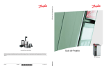
Figure 3.3: Shroud fence built around the Wind Profiler antennas
In an attempt to try to improve the isolation between the antennas and reduce the
leakage received, shrouds for the antennas were developed in order to reduce coupling.
The fence started at the ground level and reached 15 to 20 cm above the antennas.
The two antennas with shroud fence are depicted on Figure(3.3). The Wind Profiler
was tested again with the following results: The antenna isolation improved by 2
dB but the improvement in clutter rejection was insignificant. That suggested that
the main path for the clutter is not the backlobe but the antenna sidelobes. A new
redesign of the antennas or the shroud can effectively address this issue.
14
Vector Modulator
The mission of the vector modulator was to try to cancel the leakage. The Vector
Modulator is a device capable of changing the attenuation and the phase of its input
signal. With that, theoretically it should be possible to generate an opposite signal of
the leakage received. But once used in the radar the cancellation achieved was fewer
than 13dB which was not enough. Also the cancellation achieved was not the same
throughout the entire bandwidth as it would be desired. The leakage power and the
best achieved cancellation are shown in Figure(3.4).
Figure 3.4: Antenna isolation and achieved transmit leakage cancellation
Later on it was discovered that the AO card has noise of approximately the two
LSB, which was being injected to our Vector modulator. Therefore, improving the design in order to avoid using the vector modulator will improve the noise characteristics
of our receiver.
15
Proposed Solution
The low transmission power and the low antenna gain require a receiver with low
noise and very high gain. To achieve that the receiver will be redesigned avoiding the
use of the active cancellation loop. A new audio module will be created with low noise
components such as the Linear Technology, Ultralow Noise, Low Distortion, Audio
Op Amp, LT1115 [8]. The design will be totally customized for the FMCW Wind
Profiler’s needs. The front-end of the receiver will be customized too. Moreover,
a new Data Acquisition Board of 24 bits instead of 16 bits is required, and a new
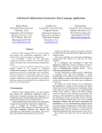
modification of the FPGA design is needed. In Figure(3.5) the new FMCW-Wind
profiler block diagram is showed. Parts in color are modified from the previous design.
16
Figure 3.5: New FMCW Wind Profiler block diagram
17
3.1.3
FMCW Radar Current State
The FMCW Wind Profiler radar is still in a developing stage. A new audio module
is currently working with the radar, the front end has been customized, and the FPGA
has been modified to enhance the radar performance, having now a 100% duty cycle
chirp. For more information about it refer to [2]. The new Data Acquisition Board
arrived and it was integrated in the radar. Data acquisition programs were developed
for it, but there are synchronization issues that should be corrected in the future.
Signal processing programs were developed for the FMCW radar, allowing the radar
to be tested in the laboratory. All information will be showed in the following sections.
3.2
Wind Profiler Subsystems
Figure(3.5) shows a simplified block diagram of the FMCW Wind Profiler. Apart
from this, there are also some other necessary components like several attenuators
to adapt the input power levels. The picture Figure(3.6) show the radar hardware
deployed in laboratory. Including the Wind Profiler boxes, computer, audio module,
and instrumentation.
Figure 3.6: Radar deployment in the laboratory
18
3.2.1
Control and Transmit Subsystem
The communication between the operator and the Wind Profiler is made through
the serial interface between the computer and the Field Programable Gate Array
Board (Altera Cyclone II EP2C20 FPGA), Figure(3.7), that generates all the radar
signals required for its proper operation. The operator stores the necessary parameters
to configure the radar in a file .conf which will be sent via serial interface to the FPGA.
That file and its parameters can be modified at any time, making the radar flexible
to operate in different contexts.
Figure 3.7: Altera Cyclone II EP2C20 FPGA
The FPGA design was developed by Iva Kostadinova and David Garrido. The
design is characterized by generating all signals in total synchronization, giving no
room for timing skews that can lead to phase wrapping in the received data. A later
modification of the FPGA was developed by David Garrido, in which the duty cycle
of the Wind Profiler was enhanced to 100%, and the signals generated were modified
19
to adjust to the last Wind Profiler configuration. For more information about the
FPGA modification design, refer to [2].
The transmitted chirp is generated by a 10-bit Digital Signal Synthesizer from
Analog Devices (AD9858 DDS). The DDS receives the needed parameters for frequency sweep generation (see Figure(3.8)) from the control subsystem. The board
uses an external 800 Mhz clock referenced to the 10 Mhz FPGA clock. The analog
mixer mixes the clock signal with the chirp centered at 115 Mhz to produce the desired product at 915 Mhz at the DDS output. The undesired mixing products are
filtered then, and the signal is amplified. A 4-way splitter is used to split the transmitted signal to the three LO inputs of the receiver mixers and to the RF high power
amplifier. The high power amplifier is a linear power solid state RF amplifier from
OPHIRrf with a gain of 50 dB. Finally a 20 dB directional coupler delivers the output
of the amplifier to the antenna and couples part of it to the calibration loop.
Figure 3.8: FPGA Control signals generation
20
Figure 3.9: Control and transmit subsystem box
3.2.2
Calibration Loop
The calibration loop allows continuous monitoring of the system performance and
gives a reference point with which to evaluate the radar sensitivity. The delay line
used is a bulk acoustic wave (BAW) delay line, with an effective delay of 2μs from
Teledyne Electronic Devices. The input of the delay line is an attenuated replica of
the transmitted signal. The output of it is coupled into the receiver chain through a
20 dB coupler. The delayed chirp produces a signal of a fixed frequency beat fb corresponding to a fixed range, different depending on the Wind Profiler’s configuration.
Some of the important specifications of the delay line are showed in Table 3.2. One of
the most important characteristics is the triple travel suppression, with a minimum
of 11 dB of suppression. That means that other fixed frequencies beat will appear at
3fb and 5fb .
21
Parameter
Center frequency
Bandwidth
Time Delay
Insertion Loss at 915 MHz
Tripple Travel Suppression
Peak Power
Value
915 MHz
25 MHz
2.000 ± 0.012μs
11.5 dB
11 dB min
100 mW
Table 3.2: Delay line specifications
3.2.3
Receiver Subsystem
The receiver subsystem consists of three identical RF paths for the three receiver
channels. The received signal is a mix of atmospheric echoes, clutter, and antenna
leakage. That leakage is orders of magnitude larger than the echoes, and it can easily
saturate the front end of the receiver. The calibration signal is also coupled to the
received signal in the front end.
Figure 3.10: Receiver subsystem box
22
The first component of the chain is a low noise amplifier in order to ensure a good
noise figure. Doing that the noise figure of the system will primarily be the noise figure
of the first few components in the receiver chain. The coupler in the Wind Profiler
is a 20 dB coupler from Narda Microwave East with insertion loss of Lcoupler = 0.3
dB. The power level of the delay line signal which is coupled into the receiver through
the coupler should be such that no extra thermal noise from the transmitted signal
gets coupled into the receiver. The LNA is a Phoenix PA911C with a noise figure of
0.9 dB. The next component in the chain is a ceramic band pass filter (BPF) from
Lark Engineering with a bandwidth of 25 MHz and insertion loss of 2.5 dB.
The Wind Profiler utilizes a high power mixer from Mini Circuits (ZEM-4300MH+)
with a 1 dB compression point of +9 dBm. The mixer has a LO power level of +13
dBm. For reliable performance, the LO level should vary no more than ±3 dBm
from its specified value. For the Wind Profiler operating frequency range, the mixer
insertion loss varies from 6 to 8 dB depending on the LO input level.
The dynamic range of the Data Acquisition Card and the expected backscattered
power from the phenomena desired to be observed are the two parameters defining the
total gain that the receiver should have. The Data Acquisition Card in the new Wind
Profiler configuration is a 24-bit 24DSI6LN from General Standards. The specified
voltage range is ±10 V corresponding to a maximum input power of 30 dBm for a
single tone. The dynamic range of the DAQ is 110 dB setting its quantization noise
floor at -80 dBm.
The audio filter in the receiver chain is a bandpass active filter designed by David
Garrido. Its design is totally customized for the Wind Profiler. To design the filter
it was important to ensure that the audio filter significantly attenuates the leakage
signal, and there is a trade off between filter ringing and desired observable minimum
heights. Because one of the primary design goals of the Wind Profiler is to be able to
23
observe boundary layer processes at low altitudes it is important to make the trade
off carefully. In Figure(3.11) the filter response to a signal composed of leakage plus
calibration signal can be observed.
Figure 3.11: Audio module filter ringing
24
CHAPTER 4
DATA ACQUISITION
After identifying the problems encountered with the Wind Profiler, it was necessary to proceed to modify the receiver and to create a new audio module totally
customized for the Wind Profiler, that will enhance its performance. The design was
done employing low-noise components to achieve a better performance, for example
the operational amplifier used was the LT1115 from Linear Technology [8], with a
√
typical voltage noise of 0.9nV / Hz at 1 kHz.
With the 16-bit Power-DAQ PD2-MFS-4-500/16 from United Electronics Industries Inc. that the former Wind Profiler configuration used, the gain needed for that
audio module must be at least of 110 dB, and the order required was order 10. During
the Summer of 2009 some audio module prototypes were built. That work showed
that it was not possible to meet the specifications needed for the Wind Profiler. The
high gain and the high order of the audio module made it unstable and distorting. The
maximum gain achieved was approximately 85 dB, but the filter was still introducing
a great amount of distortion.
The solution was to improve the dynamic range of the receiver somehow, in order
to be able to relax the specifications of the audio module. To achieve that, a new
Data Acquisition Board was bought. The board is a four-channel low-noise 24-bit
delta sigma PC104-Plus from General Standards. With that new board the dynamic
range was improved from 16 bits to 24 bits, which means a theoretical improvement
of 24 dB.
25
4.1
24DSI6LN Data Acquisition Board
The selected board for the new Wind Profiler configuration is the 24DSI6LN board
from General Standards. The board has 24 bits and 4 channels. It also has low-noise
features due to its Delta Sigma architecture. Delta Sigma architecture is based on the
technique of oversampling to reduce the noise in the band of interest, which also avoids
the use of high-precision circuits for the anti-alias filter. In Delta Sigma converters,
noise is further reduced at low frequencies, which is the band where the signal of
interest is, and it is increased at the higher frequencies, where it can be filtered. This
technique is known as noise shaping. That feature is also a disadvantage because due
to that oversampling the external input clock that can be used needs to be very fast,
specifically from 25’6 Mhz to 51’2 Mhz. With the former Wind Profiler the old DAQ
used a totally synchronized clock at the desired fs provided by the FPGA. Now a
high-speed clock is needed to do so, and the fastest clock the FPGA can provide is
at 10Mhz.
Figure 4.1: 24DSI6LN Data Acquisition Card
26
The voltage range is the same as before, being ±10 V. The board also provides
its own anti-aliasing filtering which helps to relax the audio specifications even more.
The sampling clock can be generated internally, being able to chose from 2KSPS to
200KSPS with an accuracy of 25 PPM.
The sampling of multiple channel groups can be pre-synchronized through software, or each group can be synchronized to an external hardware clock input. So, in
order to synchronize the DAQ with the transmitted chirps a synchronization signal
generated in the FPGA can be used for that purpose. An acquisition program was
developed using that external synchronization input signal feature. It was tested simulating software synchronization pulses and it worked properly. But when the real
synchronization input signal was used, it was not recognized by the DAQ. Currently
that problem is still pending to be solved, waiting for the DAQ developers to identify
the board’s problem. To be able to test the system an acquisition program without
using the external synchronization signal was developed. In order to synchronize the
data, software synchronization was used while the hardware synchronization is being
fixed.
4.2
Data Acquisition Program
The DAQ needs a C program (called “savedata.c”) to collect data. This program
configures the board according to the desired parameters, first doing a test and after
that acquiring data to a file until either the timeout specified when the program
started is reached, an error occurred, or when the program is stopped manually by
pressing “CTRL+C” in the keyboard.
This program uses some other files that are not included in this document (main.h,
savedata.h between others). The main files “savedata.c” and “main.c” are provided
and commented in Appendix A. This code also uses some specific functions for this
27
device. Further information about these functions can be found in the 24DSI6LN
linux driver manual [5].
The structure of the program is as follows. First the board is searched, identified
and selected. After that the device is opened, some data is collected in a brief test and
if the test is successful it proceeds to capture the real data. The board is configured
using the function dsi config board, then the file which will contain the data is created,
using as a filename the current time. After the file is created the program continuously
collects the data until it is terminated.
Before executing the program it is important to have started the driver. To start
the driver, login as a root user, change to the directory where the driver was installed
and execute the command “./start”. To verify that the device has been loaded execute “lsmod”. The module name 24dsi should be included in the output if driver
was started properly. To collect data, the program needs to run while the radar is
operating, so, the programs that start the radar have to be executed before.
4.3
Synchronization Program
It is necessary to synchronize the collected data in order to know when a profile
starts and stops to allow proper processing of the data in order to extract range and
doppler information from it. As explained before, the synchronization via hardware
is still being developed. So, in the meantime, synchronization via software is done.
To do so an IDL program (called “pre processing david.pro”) was created for that
purpose. The main file “pre processing david.pro” is provided and commented in
Appendix B. This program also uses other files not included in this document such
as “readcol.pro”.
The structure of the program is as follows. First of all, the file containing the
data is opened and the data stored in columns is read and stored. Then the data is
28
processed, erasing the header bits from every sample and converting the information
from hexadecimal to voltage values. After that a block size smaller than the number of
samples per profiler is created, and the synchronization of data starts. To synchronize
the data, the synchronization signal is also sampled, and so the program waits until
the synchronization channel have a transition from “0” to “1”. The synchronized
data will be stored in an .img file that will be used for processing later.
This way of synchronizing the data has its problems. The sampling clock used to
sample the data is generated inside the DAQ, because it is not possible to generate an
input clock for the DAQ fast enough to meet the DAQ requirements. That means that
the clock is not synchronized with the system. The synchronization via software relies
in sampling the synchronization signal. But, as the sample clock is not synchronized,
there will be a maximum error of ±1 sample. Because of that from now on the
only information extracted from the data will be range, because to obtain doppler
information good synchronization or a more complex data processing is needed. That
will be perfected when the Wind Profiler has been tested, and is in a later stage.
29
CHAPTER 5
SIGNAL PROCESSING
After the acquisition of data, it is necessary to process it properly to extract the
required information. In the Wind Profiler, two different kinds of information can
be extracted from the data, range and doppler velocity. In the following pages only
range information will be plotted.
5.1
Signal Processing Program
To perform the data processing, a program in IDL called “windprof process david.pro”
was developed. The program is provided and commented in Appendix C. The structure of the program is as follows. At the beginning of the program the different
parameters needed for processing such as frequency sample, number of profile average and name of the files are configured. Then the synchronized data from the input
file is stored in arrays. A Fast Fourier Transform and the chosen profile average are
done. In the next step range and doppler velocity information are extracted and
written to a file.
Figure (5.1) shows a processed signal containing leakage and calibration signal. It
can be observed that there is no trace of leakage whatsoever and that three different
tones appear. The tones are due to the architecture of the BAW delay line. The
first tone correspond to the direct path of the delay line input signal through the
delay line, the other two tones correspond to triple and the quintuple path through
the delay line. The plot also shows that the noise floor is the limit for the Wind
30
Profiler sensitivity. To improve the sensitivity a estimation of the noise floor can be
subtracted from the processed data.
Figure 5.1: Leakage and calibration signal processed
5.2
Noise Floor Estimation
In order to improve the sensitivity of the Wind Profiler, an estimation of the noise
floor can be subtracted from the data. The longer the profile average is, the greater
the improvement in sensitivity will be, specifically the theoretical improvement is
related to the following expression 10log(Nprof iles ).
In a first attempt, it was proceed to estimate the noise floor in a traditional
way, capturing the output signal of the Wind Profiler when no input signal is being
introduced to the receiver. The receiver inputs were terminated at 50 Ohms, the
calibration loop input and the LO port of the mixer were also terminated at 50
Ohms. The noise floor estimation obtained was not good enough. At low frequencies
the big differences between the real noise floor and its estimation make sensitivity
improvement not possible. In Figure(5.2) the first noise floor estimation and its
result is showed. Blue line is the received signal, red line is the noise floor estimation,
and black line is the result when the estimated noise floor is subtracted to the signal.
31
The results obtained were not as good as it was expected, the audio module output
Figure 5.2: Noise floor estimation results
noise floor is different depending on its input signal. Because of that it is necessary to
make an estimation of the leakage and introduce it in the receiver’s input in order to
obtain a good estimation of the noise floor. The commented method turned out to be
a valid procedure to estimate the noise floor. In Figure(5.3) the results obtained with
that method are shown. Now in this case the improvement of sensitivity is achieved
in all the bandwidth of interest and that improvement is also constant in throughout
the bandwidth.
5.3
Minimum Detectable Signal
After achieving the improvement of the Wind Profiler sensitivity thanks to the
good estimation of the noise floor, it is interesting to find out which is the minimum
signal that can be detected with the new noise floor level achieved. To do so, the calibration signal is attenuated until it is not detected, and the penultimate attenuation
before the Wind Profiler is unable to detect it will be the one used to calculate the
minimum detectable signal.
32
Figure 5.3: Noise floor estimation results with estimation of leakage method
In Figure(5.4) the signal before subtracting the noise floor can be observed. In
it there is apparently no calibration signal. But, in Figure(5.5) after subtracting the
noise floor it is seen how the calibration signal is now detected. Two small tones
appear in the plot, showing the direct and the triple path through the BAW delay
line that it was desirable to detect.
This minimum detectable signal corresponds to a -150 dBm signal. That minimum
detectable signal is not good enough yet because only scatter from strong echoes such
as the ones occurring in rain and snow, or high Cn2 occurring in hot humid weather can
be detected. In any case, the Wind Profiler is still being upgraded and that minimum
detectable signal will improve soon after the antenna isolation is improved, and with
that improvement the receiver will be optimized to adjust to that antenna isolation
improvement increasing gain in the front-end between other possible modifications to
enhance its performance.
33
Figure 5.4: Minimum detectable signal plot
Figure 5.5: Minimum detectable signal after subtraction of the noise floor
34
CHAPTER 6
ANTENNA ISOLATION
One of the main problems with the FMCW radars is related to the isolation
between the antennas. In FMCW radars, transmission and reception is done at
the same time using different antennas for transmission and reception, unlike pulsed
radars that transmit and receive at different times through the same antenna. Pulsed
radars have height limitation at low altitudes due to their pulsed architecture. FMCW
radars have very high resolution and small peak to average power, but the isolation
between the antennas is an important issue. In the Wind Profiler case, the isolation
between the antennas is 71 dB, but a great amount of leakage is still coupled to
the receiver thorough the side-lobes. That leakage is a limiting factor for the Wind
Profiler’s performance, not allowing the addition of enough gain in the front-end of
the receiver to avoid saturating the mixer, and requiring a complex audio module
with high order to filter the leakage and high gain to compensate for the low gain
in the front-end. So, improving the Wind Profiler’s antenna isolation will boost its
performance.
Improving the antenna isolation is complicated because the two antennas are next
to each other, and so far-field theory cannot be applied. Near-fields are difficult to
study and simulate. The solution chosen to improve the antenna isolation is the use
of new antenna shrouds created for that purpose. The design of the shrouds is based
on a NOAA design [11]. The metallic shrouds are 5 feet tall and they have openings
that are cut at 45 degrees.
35
6.1
Antenna Isolation Tests With New Shrouds
In December 2009 the new shrouds were ready to be tested on the Wind Profiler.
Measurements of antenna isolation where conducted at Tilson Farm. There were
several sources of reflection at Tilson farm, like the van were all the Wind Profiler
equipment was set, a big oak tree at 30 meters from the deployment point, and a
trailer at 15 meters. See Figure(6.1) for more details.
Figure 6.1: Tilson Farm deployment point
The transmit antenna was set as far from the van as the antenna feed cables
allowed, in order to avoid reflections as much as possible. The receiver was set between
the transmitter and the van. With that deployment an antenna measurement was
done without using the shrouds. The leakage received is showed in Figure(6.2), being
-19 dBm.
After that, the antenna isolation was measured using the shrouds. Between the
edges of the antennas shrouds there was 0.61 meters of separation, and between the
van and the receiver antenna shroud edge there was a separation of 3 meters. The
openings of the antennas were not parallel to each other, to reduce the cross-talk
between the antennas. The deployment can be observed in Figure(6.3). The results
36
Figure 6.2: Received leakage without using shrouds
of the test were successful, having -34 dBm of leakage in the receiver’s front-end, see
Figure(6.4). That means an improvement on isolation of -15 dB.
The obtained results are optimistic, -15 dB of improvement is a great result, having
into account that this measurement was still experimental. The next step will be to
obtain the maximum antenna isolation improvement that can be achieved. To do
so, several improvements can be made. The deployment point can be changed to
a place with fewer sources of reflection. Absorbers can be used in the edge of the
transmitter antenna shroud, avoiding refraction and diffraction at the shroud edge,
and so improving the isolation. Also the radar antennas need to be mounted on a
platform to maintain alightment and pointing. The shrouds openings should also
be covered with plastic, since these will enable the snow and water to slide off and
not attenuate the signals. The improvement achieved will allow more gain in the
receiver’s front-end and in the audio module translating to a better radar minimum
detectable signal.
37
Figure 6.3: Wind Profiler deployment with shrouds
Figure 6.4: Received leakage using shrouds
38
CHAPTER 7
GRAPHICAL USER INTERFACE
The operation of the Wind Profiler requires knowing how to start, configure and
manage all the different parts of the radar. For example start the Wind Profiler
sending to the FPGA the required parameters, start and stop the data collection,
and process and display the acquired data.
In order to make the Wind Profiler operation easier for future users, a graphical
user interface (GUI) was created using IDL. The purpose of it was to manage all
the Wind Profiler operations commented on above using a single window with a
friendly and easy to understand interface. During the Spring of 2009 the Wind Profiler
GUI was developed for the old configuration. To adapt the GUI to the new Wind
Profiler configuration only a few changes such as path and filename modifications will
be required when all the programs and files required for the new configuration are
definitive.
The GUI interface is presented in Figure(7.1). The GUI allows to modify the
Wind Profiler parameters directly from the interface instead of having know where
the .conf file is, open it and modify it manually. When “Radar Start” button is
pressed the parameters introduced in the left part of the GUI are stored and the Wind
Profiler is started using these parameters. It is started by executing the .c program
that processes these parameters and sends all the necessary information to the FPGA
through the serial port. When “Radar Stop” button is pressed the FPGA is reset and
with that the Wind Profiler stops. The buttons “Start Data Collection” and “Stop
39
Figure 7.1: Graphical User Interface
Data Collection”, execute and kill the data acquisition program respectively. Finally
the “Display Data” button executes the data processing program with the specified
time average, and concurrently executes the real-time display program developed by
David Garrido to display the data while its being collected and processed. The GUI
files are provided and commented in Appendix D.
40
CHAPTER 8
CONCLUSIONS
8.1
Summary
This thesis has described the FMCW Wind Profiler state as of Fall 2009. The
previous configurations and problems have been explained and then solutions provided. Thanks to the previous work done with the radar, the sources of error can be
identified and the radar receiver was upgraded in order to improve its performance.
The receiver’s front end was modified, and the leakage cancellation loop used
before is now avoided. Also a new audio module was specifically designed. The
FPGA was modified too in order to achieve a 100% duty cycle to enhance the Wind
Profiler performance.
A new Data Acquisition Card is used now to increase the dynamic range of the
radar. New data acquisition and data processing programs are developed in order to
have an operative radar. Also a graphical user interface is created to make the Wind
Profiler operator tasks easy, including making all the required operations and needed
files in a single window easy to manage.
Finally, new antenna shrouds are used to improve the antennas isolation. Tests
have been done showing improvement that led to optimistic future results.
41
8.2
Future work
The first thing that needs to be done to the Wind Profiler is to fix the synchronization issue with the Data Acquisition Card. A proper synchronization will allow the
computation of proper doppler information without having to substantially increase
the complexity of the signal processing.
New antenna isolation measurements should be done with the shrouds. Mounting
the antennas and the shrouds in a platform to maintain alightment and pointing, and
making the system mobile. Also adding absorber to the transmitter’s shroud edge
could improve the antenna isolation. Then the receiver can be modified adding more
gain in the front-end to take advantage of the antenna isolation improvement, and so
reduction of the received leakage, optimizing the Wind Profiler’s performance.
After having checked the correct performance of the Wind Profiler, real data
should be acquired from field deployments. After processing the data collected the
performance of the radar can be checked, and modifications can be added in case the
data collected is not satisfactory.
Finally, when the Wind Profiler is ready, slight modifications to the graphical user
interface and to the real-time display programs can be performed to adapt them to
the new Wind Profiler configuration.
In a second phase, it is planned to use a space antenna technique [9] to be able to
analyze horizontal winds too. These techniques can obtain more rapid wind estimates
compared to Doppler beam swinging systems. By making all of the changes mentioned
previously, the Wind Profiler should be able to operate properly.
42
APPENDIX A
DATA ACQUISITION PROGRAMS
A.1
main.c
// $Rev: 1814 $
// $Date: 2009-04-22 17:13:15 -0500 (Wed, 22 Apr 2009) $
// Program developed by David Garrido Lopez
#include <ctype.h>
#include <stdio.h>
#include <stdlib.h>
#include <string.h>
#include <time.h>
#include "main.h"
#define TRIGGER_RATE
100
#define SAMPLE_RATE
60000L
#define CHANS_ENABLED
6
// variables ****************************
static int _continuous = 0;
static int _ignore_errors = 0;
43
static int _index = 0;
static long _minute_limit = 0;
static __s32 _buffer_data[3600L];
/*****************************************
*
* Function: _parse_args
*
* Purpose:
*
* Parse the command line arguments.
*
* Arguments:
*
* argc The number of command line arguments given.
*
* argv The list of command line arguments given.
*
* Returned:
*
* >= 0 The number of errors encounterred.
*
**************************************/
static int _parse_args(int argc, char** argv)
{
char c;
44
int errs = 0;
int i;
int j;
int k;
printf("USAGE: savedata <-c> <-C> <-m#> <-n#> <index>\n");
printf("
-c
Continue testing until an error occurs.\n");
printf("
-C
Continue testing even if errors occur.\n");
printf("
-m#
Run for at most # minutes (a decimal number).\n");
printf("
index
The index of the board to access.\n");
printf(" NOTE: Hit Ctrl-C to abort continuous testing.\n");
for (i = 1; i < argc; i++)
{
if (strcmp(argv[i], "-c") == 0)
{
_continuous = 1;
_ignore_errors = 0;
continue;
}
if (strcmp(argv[i], "-C") == 0)
{
_continuous = 1;
_ignore_errors = 1;
continue;
}
45
if ((argv[i][0] == ’-’) && (argv[i][1] == ’m’) && (argv[i][2]))
{
j = sscanf(&argv[i][2], "%d%c", &k, &c);
if ((j == 1) && (k > 0))
{
_minute_limit = k;
continue;
}
errs = 1;
printf("ERROR: invalid argument: %s\n", argv[i]);
break;
}
j = sscanf(argv[i], "%d%c", &k, &c);
if ((j == 1) && (k >= 0))
{
_index = k;
continue;
}
else
{
errs = 1;
printf("ERROR: invalid board selection: %s\n", argv[i]);
46
break;
}
}
return(errs);
}
/*******************************************
*
* Function: _perform_tests
*
* Purpose:
*
* Perform the appropriate testing.
*
* Arguments:
*
* fd The handle for the board to access.
*
* Returned:
*
* >= 0 The number of errors encounterred.
*
*******************************************/
static int _perform_tests(int fd)
{
47
int errs = 0;
const char* psz;
struct tm* stm;
time_t tt;
time(&tt);
stm = localtime(&tt);
psz = asctime(stm);
gsc_label("Performing Operation");
printf("%s", psz);
errs += gsc_id_driver(fd, DSI_BASE_NAME); //Identify the driver
errs += dsi_id_board(fd, -1, NULL); //Identify the board
errs += save_data(fd);
return(errs);
}
/****************************************
*
* Function: main
*
* Purpose:
*
* Control the overall flow of the application.
*
48
* Arguments:
*
* argc The number of command line arguments.
*
* argv The list of command line arguments.
*
* Returned:
*
* EXIT_SUCCESS We tested a device.
* EXIT_FAILURE We didn’t test a device.
*
*****************************************/
int main(int argc, char *argv[])
{
int errs;
time_t exec = time(NULL);
int fd = 0;
FILE* fd_file;
long hours;
long mins;
time_t now;
int qty;
int ret = EXIT_FAILURE;
long secs;
time_t t_limit;
time_t test;
49
char datebuf[128];
char filename[128];
struct tm *today;
time_t starttime;
__s32 chans = 32;
int got;
gsc_label_init(26);
test = time(NULL);
printf("savedata - Capture and Save Data to Disk
By David Garrido(Version %s)\n", VERSION);
errs = _parse_args(argc, argv);
gsc_id_host();//Identify the host os and machine
t_limit = exec + (_minute_limit * 60);
qty = gsc_count_boards(DSI_BASE_NAME);
// Count the number of installed SI04
errs = gsc_select_1_board(qty, &_index);
//Select the board to utilize when more than one is present
if ((qty <= 0))
errs++;
gsc_label("Accessing Board Index");
printf("%d\n", _index);
50
fd = gsc_dev_open(_index, DSI_BASE_NAME);
//Perform an open on the device with the specified index.
if (fd == -1)
{
errs = 1;
printf( "ERROR: Unable to access device %d.", _index);
}
if (errs == 0)
{
ret = EXIT_SUCCESS;
errs = _perform_tests(fd);///////////////////////////
}
gsc_dev_close(_index, fd);// test finished so we close
now = time(NULL);
secs = now - test;
hours = secs / 3600;
secs = secs % 3600;
mins = secs / 60;
secs = secs % 60;
printf(" (duration %ld:%ld:%02ld)\n", hours, mins, secs);
printf("Test done!\n");
51
gsc_label("Prueba!!!!!!!!!!\n");
if ((_ignore_errors == 0) && (errs))
errs++;
if ((_minute_limit) && (now >= t_limit))
errs++;
//We finish testing and we start adqiring data
if(!errs || (_ignore_errors == 0))
{
printf("Starting adquisition!!!!!!!!!!!!!!!!\n");
fd = gsc_dev_open(_index, DSI_BASE_NAME);
dsi_config_board(fd, -1, -1, SAMPLE_RATE);
errs += _channels_profiler(fd, &chans);
//Creating the file
printf("Creating the file where the data will be stored\n");
time(&starttime);
today = localtime(&starttime);
strftime(datebuf, 128, "%Y%m%d%H%M%S", today);
sprintf(filename, "%s.dat", datebuf);
fd_file =fopen(filename, "w+b");
if (fd_file == -1)
errs = 1;
else printf("file created\n");
52
for(;;)
{
now = time(NULL);
//printf("FOR!!!!!");
errs = 0;
got = dsi_dsl_read(fd, _buffer_data, sizeof(_buffer_data)/CHANS_ENABLED);
if (got < 0)
{
errs = 1;
}
else if (got != sizeof(_buffer_data)/CHANS_ENABLED)
{
errs = 1;
printf( "FAIL <---
(got %ld samples, requested %ld)\n",
(long) got,(long) sizeof(_buffer_data)/CHANS_ENABLED);
}
else
{
errs = 0;
printf( "PASS
(%ld samples)\n",(long) sizeof(_buffer_data)/CHANS_ENABLED);
}
errs = _save_data_profiler(fd_file, chans, _buffer_data,
sizeof(_buffer_data)/CHANS_ENABLED);
if ((_minute_limit) && (now >= t_limit))
break;
53
if ((_ignore_errors == 0) && (errs))
break;
}
gsc_dev_close(_index, fd);
fclose(fd_file);
}
return(ret);
}
A.2
savedata.c
// $Rev: 1814 $
// $Date: 2009-04-22 17:13:15 -0500 (Wed, 22 Apr 2009) $
// Program developed by David Garrido Lopez
#include <ctype.h>
#include <stdio.h>
#include <stdlib.h>
#include <string.h>
#include <time.h>
#include "main.h"
// #defines ****************************
#define _1M (1024L * 1024L)
#define TRIGGER_RATE
100
#define SAMPLE_RATE
60000L
54
#define CHANS_ENABLED
6
// variables *************************
static __u32 _buffer[(SAMPLE_RATE * CHANS_ENABLED) / TRIGGER_RATE];
/*****************************************
*
* Function: _channels
*
* Purpose:
*
* Check to see how many channels the board has.
*
* Arguments:
*
* fd The handle for the board to access.
*
* chan Report the number of channels here.
*
* Returned:
*
* >= 0 The number of errors encounterred.
*
***********************************/
55
static int _channels(int fd, __s32* chans)
{
int errs;
gsc_label("Input Channels");
errs = dsi_query(fd, DSI_QUERY_CHANNEL_QTY, chans);
if (errs == 0)
printf("%ld Channels\n", (long) chans[0]);
return(errs);
}
/******************************
*
* Function: _read_data
*
* Purpose:
*
* Read data into the buffer.
*
* Arguments:
*
* fd The handle for the board to access.
*
* Returned:
*
56
* >= 0 The number of errors encounterred.
*
*****************************************/
static int _read_data(int fd)
{
int errs;
long get = sizeof(_buffer) / CHANS_ENABLED;
int got;
gsc_label("Reading");
got = dsi_dsl_read(fd, _buffer, get);
if (got < 0)
{
errs = 1;
}
else if (got != get)
{
errs = 1;
printf( "FAIL <---
(got %ld samples, requested %ld)\n",
(long) got,
(long) get);
}
else
{
errs = 0;
57
printf( "PASS
(%ld samples)\n",
(long) get);
}
return(errs);
}
/****************************************
*
* Function: _save_data
*
* Purpose:
*
* Save the read data to a text file.
*
* Arguments:
*
* fd The handle for the board to access.
*
* chan The number of channels.
*
* errs have there been any errors so far?
*
* Returned:
*
* >= 0 The number of errors encounterred.
*
58
*************************************/
static int _save_data(int fd, int chan, int errs)
{
FILE* file;
int i;
long l;
const char* name = "data.txt";
long samples = sizeof(_buffer) / CHANS_ENABLED;
gsc_label("Saving");
for (;;)
{
if (errs)
{
printf("SKIPPED
(errors)\n");
errs = 0;
break;
}
file = fopen(name, "w+b");
if (file == NULL)
{
printf("FAIL <---
(unable to create %s)\n", name);
errs = 1;
break;
59
}
for (l = 0; l < samples; l++)
{
i = fprintf(file, "
%08lX", (long) _buffer[l]);
if (i != 10)
{
printf("FAIL <---
(fprintf() failure to %s)\n", name);
errs = 1;
break;
}
if ((l % chan) == (chan - 1))
{
i = fprintf(file, "\r\n");
if (i != 2)
{
printf("FAIL <---
(fprintf() failure to %s)\n", name);;
errs = 1;
break;
}
}
}
fclose(file);
60
if (errs == 0)
printf("PASS
(%s)\n", name);
break;
}
return(errs);
}
/*************************************
*
* Function: save_data
*
* Purpose:
*
* Configure the board, then capture data to a file.
*
* Arguments:
*
* fd The handle for the board to access.
*
* Returned:
*
* >= 0 The number of errors encounterred.
*
****************************************/
61
int save_data(int fd)
{
__s32 chans = 32;
int errs = 0;
gsc_label("Capture & Save");
printf("\n");
gsc_label_level_inc();
errs += dsi_config_board_profiler(fd, -1, -1, SAMPLE_RATE);
errs += _channels(fd, &chans);
errs += _read_data(fd);
errs += dsi_ain_buf_overflow(fd, -1, DSI_AIN_BUF_OVERFLOW_TEST, NULL);
errs += dsi_ain_buf_underflow(fd, -1, DSI_AIN_BUF_UNDERFLOW_TEST, NULL);
errs += _save_data(fd, chans, errs);
gsc_label_level_dec();
return(errs);
}
/*************************************
*
* Function: dsi_config_board_profiler
*
* Purpose:
*
62
* Configure the given board using common FMCW defaults.
*
* Arguments:
*
* fd The handle to use to access the driver.
*
* index The index of the board to access. Ignore if < 0.
*
* fref This is the PLL Fref value, or -1 to use the default.
*
* fsamp This is the desired Fsamp rate, of -1 to use the default.
*
* Returned:
*
* >= 0 The number of errors encountered here.
*
****************************************/
int dsi_config_board_profiler(int fd, int index, __s32 fref, __s32 fsamp)
{
int errs = 0;
__s32 ndiv;
__s32 nrate; // Legacy
__s32 nref; // PLL
__s32 nvco; // PLL
errs += dsi_rx_io_mode (fd, index, GSC_IO_MODE_DMA, NULL);
63
errs += dsi_rx_io_overflow (fd, index, DSI_IO_OVERFLOW_CHECK, NULL);
errs += dsi_rx_io_timeout (fd, index, 30, NULL);
errs += dsi_rx_io_underflow (fd, index, DSI_IO_UNDERFLOW_CHECK, NULL);
errs += dsi_initialize (fd, index);
errs += dsi_ain_mode (fd, index, DSI_AIN_MODE_DIFF, NULL);
errs += dsi_ain_range (fd, index, DSI_AIN_RANGE_10V, NULL);
errs += dsi_ain_buf_input (fd, index, DSI_AIN_BUF_INPUT_ENABLE, NULL);
errs += dsi_ain_buf_threshold (fd, index, 128L * 1024, NULL);
errs += dsi_sw_sync_mode (fd, index, DSI_SW_SYNC_MODE_CLR_BUF, NULL);
errs += dsi_channel_order (fd, index, DSI_CHANNEL_ORDER_SYNC, NULL);
errs += dsi_data_format (fd, index, DSI_DATA_FORMAT_OFF_BIN, NULL);
errs += dsi_data_width (fd, index, DSI_DATA_WIDTH_24, NULL);
errs += dsi_init_mode (fd, index, DSI_INIT_MODE_INITIATOR, NULL);
errs += dsi_external_clock_source (fd, index, DSI_EXT_CLK_SRC_GRP_0, NULL);
errs += dsi_fref_compute (fd, index, 0, &fref);
errs += dsi_channel_group_source_all (fd, index, DSI_CH_GRP_SRC_GEN_A, 1);
errs += dsi_fsamp_compute (fd, index, 0, 0, fref, &fsamp,
&nvco, &nref, &nrate, &ndiv);
errs += dsi_rate_gen_x_nvco_all (fd, index, nvco, 1);
errs += dsi_rate_gen_x_nref_all (fd, index, nref, 1);
errs += dsi_rate_gen_x_nrate_all (fd, index, nrate, 1);
errs += dsi_rate_gen_x_ndiv_all (fd, index, ndiv, 1);
errs += dsi_fsamp_report_all (fd, index, 1, &fref);
errs += dsi_xcvr_type (fd, index, DSI_XCVR_TYPE_LVDS, NULL);
errs += dsi_auto_calibrate (fd, index);
errs += dsi_ain_buf_clear_at_boundary(fd, index);
errs += dsi_ain_buf_overflow (fd, index, DSI_AIN_BUF_OVERFLOW_CLEAR, NULL);
64
errs += dsi_ain_buf_underflow (fd, index, DSI_AIN_BUF_UNDERFLOW_CLEAR, NULL);
return(errs);
}
/***********************************
*
* Function: _save_data_profiler
*
* Purpose:
*
* Save the read data to a file, customized for te FMCW radar
*
* Arguments:
*
* Buffer The data to store
*
* chan The number of channels
*
* fd_file Th handle of the file where to store the data
*
* Returned:
*
* >= 0 The number of errors encountered here.
*
************************************/
65
int _save_data_profiler(FILE* fd_file, int chan, __s32 *buffer, long samples)
{
int i;
long l;
//long samples = sizeof(buffer)/CHANS_ENABLED;
int errs = 0;
printf("Number of samples per buffer %ld\n", samples);
gsc_label("Saving data\n");
for(l=0; l< samples; l++)
{
// Only ch0 and ch3 are included on the file to make it of a reasonable size
if((l % chan == 0)||(l % 3 == 0))
{
i = fprintf(fd_file, "
%08lX", (long) buffer[l]);
if(i != 10)
{
printf("FAIL <-- (fprintf() failure)\n");
errs=1;
break;
}
}
if((l % chan) == (chan - 1))
{
i = fprintf(fd_file, "\r\n");
if(i != 2)
{
66
printf("FAIL <-- (fprintf() failure *****)\n");
errs = 1;
break;
}
}
}
return(errs);
}
/**********************************
*
* Function: _channels_profiler
*
* Purpose:
*
* Check to see how many channels the board has.
*
* Arguments:
*
* fd The handle for the board to access.
*
* chan Report the number of channels here.
*
* Returned:
*
67
* >= 0 The number of errors encounterred.
*
***************************************/
int _channels_profiler(int fd, __s32* chans)
{
int errs;
gsc_label("Input Channels");
errs = dsi_query(fd, DSI_QUERY_CHANNEL_QTY, chans);
if (errs == 0)
printf("%ld Channels\n", (long) chans[0]);
return(errs);
}
68
APPENDIX B
SYNCHRONIZATION PROGRAM
B.1
pre processing david.pro
; Pre-processing
; Consist on synchronize the data and output a file with only data and
;a mark in every profile
;% channel 0 contains info and channel 3 contains sync
;% Save info with a mark every edge of sync signal
;% and save it in a new file dataMark.txt
;Developed by David Garrido
pro pre_processing_david, infile, ch, sync
number_channels = 6 ; currently the board has 6 channels
fs = 60000 ;define the frequency sample
PRF=100
outfile = infile + ’.img’ ; that should be modified later for ordinary data
print, outfile
lun = 1
lun_out = 2
; our input file
; our output file
69
close, /all
on_ioerror, at_eof
;jump to at_eof in case of ioerror
;
;Read the adquired data, from the infile, organized in columns
;
;Default route: ’/Users/user/Desktop/noise floor/IDL/Default/test.dat’
print, ’before data’
lines_skipped = 0
; define the number of lines skipped at the beggining of the file
FMT=’A,A’
; the structure of the data is defined, choose between the available data!!!
readcol, infile, F=FMT, ch0, ch3, SKIPLINE=lines_skipped
;the columns are saved, we can discard data using X in the format instead of A.
ch0=strmid(ch0,2,6)
; the first 8 bits are discarded, they indicated the channel only
ch3=strmid(ch3,2,6)
print, ’Data read’
;
;Conversion from hexadecimal string to double
;
size_array=size(ch0)
size_array=size_array(1)
ch_info=dblarr(size_array)
70
ReadS, ch3, ch_info, Format=’(Z)’
ch_sync=dblarr(size_array)
ReadS, ch0, ch_sync, Format=’(Z)’
ch0=’’
ch3=’’
;
;Now data should be transformed to real Voltage values.
;%1LSB equals the full escale (20V) divided by 1.1921uV (24 bits)
LSB = 20.0000000/(2.0000000^24.0000000)
ch_info=ch_info*LSB -10 ;transforming integer to real voltage value
ch_sync=ch_sync*LSB -10
ch_sync_max=max(ch_sync)
ch_sync_min=min(ch_sync)
ch_info_min=min(ch_info)
ch_info_max=max(ch_info)
ch_info_mean=mean(ch_info)
ch_sync_mean=mean(ch_sync)
print, ’ch_sync: ’, ch_sync_max, ch_sync_min, ch_sync_mean,
’
ch_info: ’, ch_info_max, ch_info_min, ch_info_mean
;
; Synchronize file and write the blocks to the file
;
openw,lun_out,outfile
; open the file/file descriptors
threshold = 1.65
71
; 1.65 volts are chosen, sync signal ideally between 0 and 3.3V
Block_size=double(fs/PRF) - 2 ; It is needed to do that authomatically
;due to the no synchronization or jitter,
;the minimum block size will be fs/PRF-1 to be sure I put -2
writeu, lun_out, Block_size-200
; We indicate what size_block the file will have
;so processing will be faster
if ch_sync(0) lt threshold then aux=0 else aux=1
;aux indicate the logic level, so we look for 0 to 1 transitions
last_trig=0
for index =0L, size_array-1 do begin
; in that for we look for trigger,
;in order to synchronize data and save to the file
; last block should be discarded, to do so last_trig variable is used
if aux eq 0 then begin
if ch_sync(index) gt threshold then begin
aux=1
if last_trig gt 0 then begin
writeu, lun_out, ch_info[last_trig+110:last_trig+Block_size-1-90]
if index-last_trig lt Block_size then print, ’Sync error’
;make sure the block are really block_size long at least
endif
last_trig=index
72
endif
endif else begin
if ch_sync(index) lt threshold then aux=0
endelse
endfor
print, ’Marked file created!!!!!!!!’
at_eof:
close,lun
close,lun_out
Block_size=’’
ch_sync=’’
ch_info=’’
print, ’File created.’
end
73
APPENDIX C
SIGNAL PROCESSING PROGRAM
C.1
windprof process david.pro
;Developed by David Garrido Lopez, UMass Amherst, MIRSL 2009
;That program process the data already saved into infile
;in blocks by pre_processing_david.pro
;
Steps for FMCW Processing
; 1. read header, creating a structure
; 2. read profile and convert data to time domain using fft
; 3. remove temporal mean to get rid of stationary targets such as
;
buildings and trees..
; 4. get power and average in time
pro windprof_process_david, infile
lun = 1
lun_out = 2
lun_noise = 3
close, lun, lun_out, lun_noise
lambda=3e8/915e6
74
prof_avg = 10000
; here we decide how many profiles we’re gonna average
size_sample=8 ; A double has 8 bytes so does a sample
number_channels=1
; number of channels on the file to process (not on the board)
sample_freq=60000 ; sample frequency
outfile = infile + ’.fig’ ; that should be modified later for ordinary data
ch=0 ; By now only one channel
prf=100
on_ioerror, at_eof
openr, lun_noise,
’/Users/user/Desktop/noise floor/IDL/Default/noise_5min_ampnewfilter2.img.fig’
print, ’noise opened’
openw, lun_out, outfile
openr, lun ,infile
info=fstat(lun)
Block_size=double(0)
readu, lun, Block_size
total_samples = info.size/size_sample
total_profiles = (total_samples -1)/(Block_size*number_channels)
print, ’Total profiles in file:
’, total_profiles
; once it is known how many profiles there are on the file,
;it is proceed to process it
75
f_frame=dblarr(Block_size, prof_avg)
rawdata = dblarr(number_channels,Block_size)
wsamples=Block_size
windw = rebin(hanning(wsamples), wsamples, prof_avg)
winfunc=dblarr(Block_size,prof_avg)
winfunc[0:wsamples-1,*]=windw
;;;;;;;;;;;;;;;;;;;;;;;;;;;;;;;;;;;;;;;;;;;;;;;;;
;
;First noise mean, estimated from 10 minutes noise file
;
;;print, fstat(lun_noise)
pow1_noise=dblarr(199)
readu, lun_noise, pow1_noise
mean_noise=mean(pow1_noise[50:198])
; the mean is found substracting the first samples
;because at low frequencies there’s no noise due to the filter response
print, ’mean =
’
mean2:
’, mean(pow1_noise), ’
maximum:
’, max(pow1_noise),
’, mean(pow1_noise[50:198])
;;;;;;;;;;;;;;;;;;;;;;;;;;;;;;;;;;;;;;;;;;;;;;;;;;;;;;;;;;;;;;;;;;;;;;;
for avg_frame_index=0L, total_profiles/prof_avg-1
for frame_index= 0L, prof_avg-1 do begin
readu,1,rawdata
rawdata=rawdata
f_frame[*,frame_index] = rawdata(ch,*)
endfor
f_frame=f_frame*winfunc
76
do begin ;big loop
c_frame=(fft(f_frame,dimension=1))[0:Block_size/2-1,*];
c_mean=total(c_frame,2)/prof_avg
c_frame1=c_frame-complex(rebin(real_part(c_mean),Block_size/2, $
prof_avg),rebin(imaginary(c_mean),Block_size/2, prof_avg))
pow=total(double(c_frame*conj(c_frame)), 2)/prof_avg
pow1=(total(double(c_frame1*conj(c_frame1)), 2)/prof_avg)
autocorr=total(c_frame[*,1:prof_avg-1]* $
conj(c_frame[*,0:prof_avg-2]),2) / (prof_avg-1)
autocorr_phase=atan(autocorr,/phase)
autocorr1=total(c_frame1[*,1:prof_avg-1]* $
conj(c_frame1[*,0:prof_avg-2]),2) / (prof_avg-1)
autocorr_phase1=atan(autocorr1,/phase)
;Get velocity
vel=autocorr_phase*(prf*lambda)/(4*!pi)
vel1=autocorr_phase1*(prf*lambda)/(4*!pi)
;Get coherence
rho=abs(autocorr)/pow
rho1=abs(autocorr1)/pow1
;powdb=10*alog10(pow)
77
;powdb1=10*alog10(pow1)
;writeu,lun_out,pow,vel,rho,c_mean
writeu,lun_out,pow1,vel1,rho1,c_mean
endfor
;;print, fstat(lun_out)
size_pow1=size(pow1)
noise_avg=28500 ;58400
std=mean_noise/sqrt(noise_avg)
pow1_plot=pow1
xant=1e-6
for index=0L, size_pow1(3)-1
do begin
x=pow1(index)-pow1_noise(index)*0.80
if x lt 0 then begin
;x=abs(x)
;if xant-x le 0 then x=xant+x*0.1 else x=xant-x*0.1
endif
pow1_plot(index)=x
xant=x
endfor
;window, 0
;plot, rawdata
window, 4
plot, 10*alog10(pow1_plot)+30, xtitle=’samples’, ytitle=’Power(dBm)’
78
for index2=0L, size_pow1(3)-1
do begin
if pow1_plot(index2) lt pow1_noise(index2)-4*std then pow1_plot(index2)=1e-10
endfor
;oplot, 10*alog10(pow1_plot)+30, COLOR=1500
oplot, 10*alog10(pow1) + 30, COLOR=’00FFFF’x
oplot, 10*alog10(pow1_noise) + 30, COLOR=’FFFF00’x
print, ’std: ’, std
at_eof:
close,lun
close,lun_out
close, lun_noise
print, ’File created.’
end
79
APPENDIX D
GRAPHICAL USER INTERFACE PROGRAM
D.1
wgui fmcw create.pro
; David Garrido Lopez
; MIRSL Lab @ UMass Amherst
;
; GUI For FMCW Boundary layer radar
;
PRO wgui_fmcw_create
COMMON SHARE1, hdr, display, datafile, lun
display=1
;datafile=’fmcw.conf’
;hdr = header_w()
base = widget_base(title=’UMass FMCW Radar GUI v1.0’, /row)
;
;
Positioner settings
;
80
b0 = widget_base(base, /frame, /column)
t0 = widget_label(b0, value="-- Radar Settings --")
b1 = widget_base(b0, /row)
t2 = widget_label(b1, value=’Center frequency:
’)
t2 = widget_text(b1, /editable, xsize=8, uname=’centr_freq’, value=’115’)
t2 = widget_label(b1, value=’[Mhz]’)
b1 = widget_base(b0, /row)
t2 = widget_label(b1, value=’Bandwidth:
’)
t2 = widget_text(b1, /editable, xsize=8, uname=’bw’, value=’25’)
t2 = widget_label(b1, value=’[Mhz]’)
b1 = widget_base(b0, /row)
t2 = widget_label(b1, value=’Chirp lenght:
’)
t2 = widget_text(b1, /editable, xsize=8, uname=’chirp_time’, value=’8.3333’)
t2 = widget_label(b1, value=’[mseg]’)
b1 = widget_base(b0, /row)
t2 = widget_label(b1, value=’PRF:
’)
t2 = widget_text(b1, /editable, xsize=8, uname=’prf_time’, value=’100’)
t2 = widget_label(b1, value=’[Hz]’)
b1 = widget_base(b0, /row)
t2 = widget_label(b1, value=’AO sampling freq:
’)
t2 = widget_text(b1, /editable, xsize=8, uname=’AO_freq’, value=’40’)
81
t2 = widget_label(b1, value=’[Khz]’)
b1 = widget_base(b0, /row)
t2 = widget_label(b1, value=’Sample frequency:
’)
t2 = widget_text(b1, /editable, xsize=8, uname=’samp_freq’, value=’61’)
t2 = widget_label(b1, value=’[Khz]’)
b1 = widget_base(b0, /row)
t2 = widget_label(b1, value=’Scans per profile: ’)
t2 = widget_text(b1, /editable, xsize=8, uname=’scans_profile’, value=’610’)
t2 = widget_label(b1, value=’[]’)
b1 = widget_base(b0, /row)
t2 = widget_label(b1, value=’Total profile:
’)
t2 = widget_text(b1, /editable, xsize=8, uname=’profile’, value=’180000’)
t2 = widget_label(b1, value=’[]’)
b1 = widget_base(b0, /row)
t2 = widget_label(b1, value=’Scans per frame:
’)
t2 = widget_text(b1, /editable, xsize=8, uname=’scans_frame’, value=’30500’)
t2 = widget_label(b1, value=’[]’)
b1 = widget_base(b0, /row)
t2 = widget_label(b1, value=’Number of channels:’)
t2 = widget_text(b1, /editable, xsize=8, uname=’channels’, value=’3’)
t2 = widget_label(b1, value=’[channels]’)
82
;
;
Radar buttons
;
b1 = widget_base(base, /frame, /column)
t0 = widget_label(b1, value=’-- Radar configuration --’)
b2 = widget_button(b1, value=’Radar Start’, uname="radar_start", $
uvalue="radar_start")
b2 = widget_button(b1, value=’Radar Stop’, uname="radar_stop", $
uvalue="radar_stop")
t2 = widget_label(b1, value="-- Data collection --")
b2 = widget_button(b1, value=’Start Data Collection’, uname="data_start", $
uvalue="data_start")
b2 = widget_button(b1, value=’Stop Data Collection’, uname="data_stop", $
uvalue="data_stop")
;b1 = widget_base(base, /frame, /column)
t2 = widget_label(b1, value="-- Display Data --")
b2 = widget_base(b1, /row)
t2 = widget_label(b2, value=’Time Average:
’)
t2 = widget_text(b2, /editable, xsize=8, uname=’time_avg’, value=’61’)
t2 = widget_label(b2, value=’[s]’)
83
b2 = widget_button(b1, value=’Display Data ’, uname="display_data", $
uvalue="display_data")
setenv, ’INIT=1’
widget_control, base, /realize
xmanager, ’wgui_fmcw’, base
END
D.2
wgui fmcw event.pro
; David Garrido Lopez
; MIRSL Lab @ UMass Amherst
;
; GUI For FMCW Boundary Layer Radar
;
PRO wgui_fmcw_event, ev
COMMON SHARE1, hdr, display, datafile, lun
value=0L
widget_control, ev.id, get_uvalue=value
case (value) of
"radar_stop": begin
84
print, "radar stop!"
close,1 ;For testing purposes, debug etc etc
close,2 ;For testing purposes, debug etc etc
reset
return
end
"radar_start": begin
print, ’radar start!’
get_conf_file, ev ; create the .conf file
run_windprofiler
; executes windprofiler.c and inits radar (fpga)
return
end
"data_stop": begin
print, ’data acquisition stop!’
spawn, ’sudo killall -s TERM fmcwsa’
return
end
"data_start": begin
print, ’data acquisition start!’
run_daq
; inits data acquisition
return
end
"display_data": begin
85
print, ’displaying data!’
windprof_oldaq
windprof_oldaqdisp
return
end
else: return
endcase
return
END
D.3
get conf file.pro
pro get_conf_file, ev
;
; Creating the fmcw.conf file
;
openw,1,’/Users/user/Desktop/PFC/IDL/FMCW/WindProfiler_Last/fmcw_prueba.conf’
;specify the concrete rute!!!!!!!
openw,2,’/Users/user/Desktop/PFC/IDL/FMCW/RunDaq/fmcw_prueba.conf’
;specify the concrete rute!!!!!!!
id = widget_info(ev.top, find_by_uname=’centr_freq’)
widget_control, id, get_value=centr_freq
86
printf,1,’Center Frequency (MHz) :’,centr_freq
printf,2,’Center Frequency (MHz) :’,centr_freq
id = widget_info(ev.top, find_by_uname=’bw’)
widget_control, id, get_value=bw
printf,1,’Bandwidth (MHz)
:’,bw
printf,2,’Bandwidth (MHz)
:’,bw
id = widget_info(ev.top, find_by_uname=’chirp_time’)
widget_control, id, get_value=chirp_time
printf,1,’Chirp Length(ms) :’,chirp_time
printf,2,’Chirp Length(ms) :’,chirp_time
id = widget_info(ev.top, find_by_uname=’prf_time’)
widget_control, id, get_value=prf_time
printf,1,’PRF (Hz)
:’,prf_time
printf,2,’PRF (Hz)
:’,prf_time
id = widget_info(ev.top, find_by_uname=’AO_freq’)
widget_control, id, get_value=AO_freq
printf,1,’AO Sample Frequeny(kHz) :’,AO_freq
printf,2,’AO Sample Frequeny(kHz) :’,AO_freq
id = widget_info(ev.top, find_by_uname=’samp_freq’)
widget_control, id, get_value=samp_freq
printf,1,’Sample Frequency (kHz) :’,samp_freq
printf,2,’Sample Frequency (kHz) :’,samp_freq
id = widget_info(ev.top, find_by_uname=’scans_profile’)
widget_control, id, get_value=scans_profile
printf,1,’Scans per Profile
:’,scans_profile
printf,2,’Scans per Profile
:’,scans_profile
id = widget_info(ev.top, find_by_uname=’profile’)
87
widget_control, id, get_value=profile
printf,1,’Total Profiles
:’,profile
printf,2,’Total Profiles
:’,profile
id = widget_info(ev.top, find_by_uname=’scans_frame’)
widget_control, id, get_value=scans_frame
printf,1,’Scans Per Frame
:’,scans_frame
printf,2,’Scans Per Frame
:’,scans_frame
id = widget_info(ev.top, find_by_uname=’channels’)
widget_control, id, get_value=channels
printf,1,’Number of Channels :’,channels
printf,2,’Number of Channels :’,channels
close,1
close,2
end
D.4
run windprofiler.pro
pro run_windprofiler
;
; Compile and execute windprofiler.c, that inits the radar!
;
spawn, ’g++ -o /Users/user/Desktop/PFC/IDL/FMCW/WindProfiler_Last/windprofiler
/Users/user/Desktop/PFC/IDL/FMCW/WindProfiler_Last/windprofiler.c’
print, ’windprofiler compiled’
spawn, ’sudo ./Users/user/Desktop/PFC/IDL/FMCW
88
/WindProfiler_Last/windprofiler fmcw.conf’
print, ’windprofiler executed’
end
D.5
reset.pro
pro reset
;
; Compile and execute reset.c, which stops radar!
;
spawn, ’g++ -o /Users/user/Desktop/PFC/IDL/FMCW/WindProfiler_Last
/reset
/Users/user/Desktop/PFC/IDL/FMCW/WindProfiler_Last/reset.c’
print, ’reset compiled’
spawn, ’sudo ./Users/user/Desktop/PFC/IDL/FMCW/WindProfiler_Last/reset ’
print, ’reset executed’
end
D.6
run daq.pro
pro run_Daq
;
; Compile and execute fmcwsa.c, that inits the data acquisition!
89
;
spawn, ’g++ -o /Users/user/Desktop/PFC/IDL/FMCW/RunDaq/fmcwsa
/Users
/user/Desktop/PFC/IDL/FMCW/RunDaq/fmcwsa.c’
print, ’fmcwsa compiled’
spawn, ’sudo ./Users/user/Desktop/PFC/IDL/FMCW/RunDaq/fmcwsa fmcw.conf’
print, ’fmcwsa executed’
end
90
BIBLIOGRAPHY
[1] David Atlas.“Radar in Metrology”. American Meteorological Society, Boston,
1990.
[2] David Garrido Lopez.“An UHF Frequency-Modulated Continous Wave Wind
Profiler - Receiver and Audio Module Development”. Master’s Thesis, University
of Massachusetts at Amherst, 2009
[3] David M. Pozar.“Microwave and RF Design of Wireless Systems”. John Wiley
& Sons, 2001.
[4] Earl E. Gossard.“Refractive index variance and its height distribution in different
air masses”. Radio Science 12, 1977.
[5] General Standards Corporation“24DSI Linux Device User Manual”. Datasheet.
[6] Iva Kostadinova.“An UHF Frequency-Modulated Continous Wave Wind Profiler - Developement and Initial Results”. Master’s Thesis, University of Massachusetts at Amherst, 2009
[7] Liam E. Gumley.“practical IDL programming”. Morgan Kaufmann, San Diego,
2002.
[8] Linear Technology“Ultralow Noise, Low Distortion, Audio Op Amp, LT1115”.
Datasheet.
[9] Muschinski, A., S.J. Frasier, “Supplement to Investigation of Turbulence and
Intermittency in the Convective Boundary Layer Using a 915MHz Volume Wind
Profiler’: Profiler Fabrication”, 2006
[10] Ottersen H.“Atmospheric structure and radar backscattering in clear air”. Radio
Science 4, 12 (1969), 1179-1193.
[11] Paul E. Johnston, David A. Carter, James R. Jordan, Allen B. White, “A New
Snow-Level Detection Radar”, NOAA 2009
[12] Turker, Frasier, S., Muschinski, A., and Pazmany, A. An s-band fmcw boundary
layer profiler: Description and initial results. “Radio Science 38”, 4 (2003).
91