1
Telemark University College
Department of Electrical Engineering, Information Technology and Cybernetics
So You Think You Can
MathScript
HANS-PETTER HALVORSEN, 2011.09.21
Part II: Dynamic Systems
Faculty of Technology, Postboks 203, Kjølnes ring 56, N-3901 Porsgrunn, Norway. Tel: +47 35 57 50 00 Fax: +47 35 57 54 01
Preface
Purpose with this Lab
In this lab you will learn how to use a tool like MathScript (which has a similar syntax as MATLAB) to
solve control and simulation problems.
In this assignment you will define and simulate dynamic systems using:
Block Diagrams
Transfer functions
State-space models
Time delay and Pade’ approximations
For additional information and resources:
http://home.hit.no/~hansha/?lab=mathscript
Note! For all the tasks in this document you should use the Script Window (Not the Command
Window). When you use the Script Window you can save
the code as an .m file. In the Script
Window we can enter several commands in a sequence and save them as a file. You execute these
script files by clicking the green arrow
in the toolbar. This way you can easily save each task as
an separate .m file (e.g., task1.m, task2.m, etc.).
ii
MathScript
MathScript is a high-level, text- based programming language. MathScript includes more than 800
built-in functions and the syntax is similar to MATLAB. You may also create custom-made m-file like
you do in MATLAB.
MathScript is an add-on module to LabVIEW but you don’t need to know LabVIEW programming in
order to use MathScript.
What is LabVIEW?
LabVIEW (short for Laboratory Virtual Instrumentation Engineering Workbench) is a platform and
development environment for a visual programming language from National Instruments. The
graphical language is named "G".
What is MATLAB?
MATLAB is a tool for technical computing, computation and visualization in an integrated
environment. MATLAB is an abbreviation for MATrix LABoratory, so it is well suited for matrix
manipulation and problem solving related to Linear Algebra.
MATLAB offers lots of additional Toolboxes for different areas such as Control Design, Image
Processing, Digital Signal Processing, etc.
What is MathScript?
iii
MathScript is a high-level, text- based programming language. MathScript includes more than 800
built-in functions and the syntax is similar to MATLAB. You may also create custom-made m-file like
you do in MATLAB.
MathScript is an add-on module to LabVIEW but you don’t need to know LabVIEW programming in
order to use MathScript. If you want to integrate MathScript functions (built-in or custom-made
m-files) as part of a LabVIEW application and combine graphical and textual programming, you can
work with the MathScript Node.
In addition to the MathScript built-in functions, different add-on modules and toolkits installs
additional functions. The LabVIEW Control Design and Simulation Module and LabVIEW Digital
Filter Design Toolkit install lots of additional functions.
You can more information about MathScript here: http://www.ni.com/labview/mathscript.htm
How do you start using MathScript?
You need to install LabVIEW and the LabVIEW MathScript RT Module. When necessary software is
installed, start MathScript by open LabVIEW:
In the Getting Started window, select Tools -> MathScript Window...:
iv
v
Table of Contents
Preface......................................................................................................................................................ii
Purpose with this Lab ...........................................................................................................................ii
MathScript...........................................................................................................................................iii
Table of Contents .................................................................................................................................... vi
1
Control Design in MathScript.......................................................................................................... 8
2
Transfer Functions .......................................................................................................................... 9
3
4
5
2.1
Introduction ............................................................................................................................. 9
2.2
First order Transfer Functions ............................................................................................... 11
2.3
Second order Transfer Functions .......................................................................................... 13
2.4
Block Diagrams ...................................................................................................................... 15
2.5
PID ......................................................................................................................................... 17
2.6
Analysis of Standard Functions ............................................................................................. 18
State-space Models ...................................................................................................................... 22
3.1
Introduction ........................................................................................................................... 22
3.2
Tasks ...................................................................................................................................... 23
Time-delay and Pade’-approximations ......................................................................................... 26
4.1
Introduction ........................................................................................................................... 26
4.2
Tasks ...................................................................................................................................... 31
Stability Analysis ........................................................................................................................... 33
5.1
Introduction ........................................................................................................................... 33
5.2
Poles ...................................................................................................................................... 34
5.3
Tasks ...................................................................................................................................... 35
5.4
Feedback Systems ................................................................................................................. 36
vi
vii
6
Table of Contents
Additional Tasks ............................................................................................................................ 39
Appendix A – MathScript Functions ...................................................................................................... 40
MathScript - Part II: Dynamic Systems
1 Control Design in
MathScript
In this task you will learn how to use MathScript for Control Design and Simulation. We will learn to
create transfer functions and state-space models and simulate such systems. We will also learn how
to implement systems with time-delay using Pade’ approximations.
Note! Using LabVIEW MathScript for Control Design purposes you need to install the
“Control Design and Simulation Module” in addition to the “MathScript RT Module” itself.
Type “help cdt” in the Command Window in the MathScript environment and the LabVIEW Help
window appears:
Use the Help window and read about some of the functions available for control design and
simulation.
8
2 Transfer Functions
2.1 Introduction
Transfer functions are a model form based on the Laplace transform. Transfer functions are very
useful in analysis and design of linear dynamic systems.
A general Transfer function is on the form:
( )
( )
( )
Where
is the output and
is the input.
MathScript has several functions for creating transfer functions:
Function
tf
Sys_order1
Sys_order2
pid
Description
Example
Creates system model in transfer function form. You also can
use this function to state-space models to transfer function
form.
Constructs the components of a first-order system model based
on a gain, time constant, and delay that you specify. You can use
this function to create either a state-space model or a transfer
function model, depending on the output parameters you
specify.
Constructs the components of a second-order system model
based on a damping ratio and natural frequency you specify. You
can use this function to create either a state-space model or a
transfer function model, depending on the output parameters
you specify.
Constructs a proportional-integral-derivative (PID) controller
model in either parallel, series, or academic form. Refer to the
LabVIEW Control Design User Manual for information about
these three forms.
>num=[1];
>den=[1, 1, 1];
>H = tf(num, den)
>K = 1;
>tau = 1;
>H = sys_order1(K, tau)
>dr = 0.5
>wn = 20
>[num, den] = sys_order2(wn, dr)
>SysTF = tf(num, den)
>Kc = 0.5;
>Ti = 0.25;
>SysOutTF = pid(Kc, Ti,
'academic');
A general transfer function can be written on the following general form:
( )
( )
( )
The Numerators of transfer function models describe the locations of the zeros of the system, while
the Denominators of transfer function models describe the locations of the poles of the system.
In MathScript we can define such a transfer function using the built-in tf function as follows:
num=[bm, bm_1, bm_2, … , b1, b0];
den=[an, an_1, an_2, … , a1, a0];
9
10
Transfer Functions
H = tf(num, den)
Example:
1. Given the following transfer function:
( )
MathScript Code:
num=[2, 3, 4];
den=[5, 9];
H = tf(num, den)
2. Given the following transfer function:
( )
MathScript Code:
num=[4, 0, 0, 3, 4];
den=[5, 0, 9];
H = tf(num, den)
Note! If some of the orders are missing, we just put in zeros. The transfer function above can be
rewritten as:
( )
3. Given the following transfer function:
( )
We need to rewrite the transfer function to get it in correct orders:
( )
MathScript Code:
num=[2, 3, 7];
den=[6, 5, 0];
H = tf(num, den)
MathScript - Part II: Dynamic Systems
11
Transfer Functions
[End of Example]
Below we will learn more about 2 important special cases of this general form, namely the 1.order
transfer function and the 2.order transfer function.
2.2 First order Transfer Functions
A first order transfer function is given on the form:
( )
Where
is the Gain
is the Time constant
Example:
Given the following transfer function:
( )
In MathScript we will use the following code:
num=[1];
den=[1, 1];
H = tf(num, den)
We divide the transfer function in numerator and denominator, and then we use the built-in tf
function.
We enter the code shown above in the Script window as shown below:
MathScript - Part II: Dynamic Systems
12
Transfer Functions
We can also use the sys_order1 function:
K = 1;
T = 1;
H = sys_order1(K, T)
[End of Example]
Step Response:
The step response for a 1.order transfer function is as follows (a step
at
):
The time constant T is defined as the time where the response reaches 63% of the steady state value.
Task 1: Transfer function
→ Use the tf function in MathScript to define the transfer function below:
( )
Set
and
.
→ Define the same function using the sys_order1 function.
→ Find also the step response for the system using the built-in step function.
Note! In this task and the subsequent tasks, you should use the Script Window (Not the Command
Window). When you use the Script Window you can save the code as an .m file. In the Script Window
we can enter several commands in a sequence and save them as a file.
MathScript - Part II: Dynamic Systems
13
Transfer Functions
[End of Task]
2.3 Second order Transfer Functions
A second order transfer function is given on the form:
( )
(
)
Where
is the gain
zeta is the relative damping factor
[rad/s] is the undamped resonance frequency.
Theory: 2.order Systems
Example:
Given the following system:
( )
MathScript Code:
num=[1 2 3];
den=[4 1];
H=tf(num,den)
This gives the following output in MathScript:
[End of Example]
MathScript - Part II: Dynamic Systems
14
Transfer Functions
Step Response:
For a 2.order system we have the following step responses depending on
:
Task 2: 2.order
→ Define the transfer function below using the tf and the sys_order2 functions (2 different methods
that should give the same results).
( )
(
)
Set
→ Plot the step response (use the step function in MathScript) for different values of
follows:
MathScript - Part II: Dynamic Systems
. Select
as
15
Transfer Functions
→ Explain the results.
Do you get the same results using tf() and sys_order2()?
[End of Task]
Task 3: Step Response
Given the following system:
( )
→ Plot the time response for the transfer function using the step function. Let the time-interval be
from 0 to 10 seconds, e.g., define the time vector like this:
t=[0:0.01:10]
and use
step(H,t)
→ Find poles and zeros for the system. Plot these into the complex plane. Tip! Use the built-in
functions poles, zero and pzgraph.
→ Discuss the results
[End of Task]
2.4 Block Diagrams
MathScript have built-in functions for manipulating block diagrams and transfer functions.
Serial:
MathScript:
…
H = series(h1,h2)
MathScript - Part II: Dynamic Systems
16
Transfer Functions
Parallel:
MathScript:
…
H = parallel(h1,h2)
Feedback:
MathScript:
…
H = feedback(h1,h2)
Task 4: Transfer functions and Block Diagrams
Use the series, parallel and feedback functions in MathScript on the block diagrams below:
→ Find the transfer function
( )
( )
( )
from the following block diagram:
MathScript - Part II: Dynamic Systems
17
Transfer Functions
→ Find the transfer function
( )
( )
( )
from the following block diagram:
→ Find the transfer function
( )
( )
( )
from the following block diagram:
→ Find the step response for these systems.
[End of Task]
2.5 PID
Currently, the Proportional-Integral-Derivative (PID) algorithm is the most common control algorithm
used in industry.
The PID controller calculates the controller action,
( )
( ):
∫
̇
Task 5: PI Controller
→ Create a transfer function for a PI controller using both the built-in pid function and the tf function
in MathScript.
Do you get the same results?
MathScript - Part II: Dynamic Systems
18
Transfer Functions
Tip! When using the tf function you need to find the transfer function for a PI controller using
Laplace on the equation:
( )
∫
Given the following system:
Where
is the PI controller,
is the process and
is a low-pass filter.
→ Use the step function in MathScript in order to plot the step response of the system.
Try with different values for
and
in order to get a good result.
[End of Task]
2.6 Analysis of Standard Functions
Here we will take a closer look at the following standard functions:
1. Order system
2. Order system
Task 6: 1.order system
1.order system:
The transfer function for a 1. order system is as follows:
( )
→ Find the pole(s)
→ Plot the Step response. Use the step function in MathScript.
MathScript - Part II: Dynamic Systems
19
Transfer Functions
Step response 1: Use different values for
Step response 2: Use different values for
, e.g.,
, e.g.,
. Set
. Set
Discuss the result
→ (optional) Find the mathematical expression for the step response ( ( )). Use “Pen & Paper” for
this Assignment.
( )
( ) ( )
Where
( )
Tip! Use inverse Laplace and find the corresponding transformation pair in order to find
( )).
Use the mathematical expression you found for the step response ( ( )) and Simulate it in
MathScript using, e.g., For Loop. Compare the result with the result from the step function.
→ Create a simple sketch of step response where you mark K, U and T (
Discuss the result
[End of Task]
Task 7: 2.order system
2.order system:
The transfer function for a 2. order system is as follows:
( )
(
)
Where
is the gain
zeta is the relative damping factor
[rad/s] is the undamped resonance frequency.
→ Find the pole(s)
MathScript - Part II: Dynamic Systems
)
20
Transfer Functions
→ Plot the Step response: Use different values for
Use the step function in MathScript.
, e.g.,
. Set
and
.
Discuss the results
[End of Task]
Task 8: 2.order system – special case
Special case: When
and the poles are real and distinct we have:
( )
(
)(
)
We see that this system can be considered as two 1.order systems in series.
( )
( )
( )
(
) (
)
(
)(
)
→ Find the pole(s)
→ Plot the Step response. Set
,
function in MathScript.
. Set
,
,
,
,
. Use the step
Tip! Use the conv or the series together with the tf function in order to define the system.
Compare and discuss the results.
→ (optional) Find the mathematical expression for the step response ( ( )). Use “Pen & Paper” for
this Assignment.
( )
( ) ( )
Where
( )
Tip! Use inverse Laplace and find the corresponding transformation pair in order to find
( )).
→ Use the mathematical expression you found for the step response ( ( )) and Simulate it in
MathScript using, e.g., For Loop. Compare the result with the result from the step function.
Discuss the results
MathScript - Part II: Dynamic Systems
21
Transfer Functions
[End of Task]
MathScript - Part II: Dynamic Systems
3 State-space Models
3.1 Introduction
A state-space model is a structured form or representation of a set of differential equations.
State-space models are very useful in Control theory and design. The differential equations are
converted in matrices and vectors, which is the basic elements in MathScript.
A general linear State-space model is on the form:
̇
MathScript has several functions for creating state-space models:
Function
ss
Sys_order1
Sys_order2
Description
Example
Constructs a model in state-space form. You also can use this
function to convert transfer function models to state-space
form.
Constructs the components of a first-order system model based
on a gain, time constant, and delay that you specify. You can use
this function to create either a state-space model or a transfer
function model, depending on the output parameters you
specify.
Constructs the components of a second-order system model
based on a damping ratio and natural frequency you specify. You
can use this function to create either a state-space model or a
transfer function model, depending on the output parameters
you specify.
Example:
Given the following state-space model:
̇
[ ]
̇
*
+* +
[
]* +
The MathScript code for implementing the model is:
%
A
B
C
Creates a state-space model
= [1 2; 3 4];
= [0; 1];
= [1, 0];
22
* +
>A = [1 2; 3 4]
>B = [0; 1]
>C = B'
>ssmodel = ss(A, B, C)
>K = 1;
>T = 1;
>H = sys_order1(K, T)
>dr = 0.5
>wn = 20
>[A, B, C, D] = sys_order2(wn, dr)
>ssmodel = ss(A, B, C, D)
23
State-space Models
D = [0];
model = ss(A, B, C, D)
[End of Example]
Theory: State-Space Models
3.2 Tasks
Task 9: State-space model
Given a mass-spring-damper system:
Where c=damping constant, m=mass, k=spring constant, F=u=force
The state-space model for the system is:
̇
[ ]
̇
[
]* +
[
[ ]
]* +
→ Define the state-space model above using the ss function in MathScript.
Step Response:
→ Apply a step in u and use the step function in MathScript to simulate the result.
Start with
,
,
, then explore with other values.
MathScript - Part II: Dynamic Systems
24
State-space Models
Conversion:
→ Convert the state-space model defined in the previous task to a transfer function using MathScript
code.
[End of Task]
Task 10:
Equations
→ Implement the following equations as a state-space model in MathScript:
̇
̇
→ Find the transfer function(s) from the state-space model using MathScript code.
→ Plot the Step Response for the system
Discuss the results.
[End of Task]
Task 11:
Block Diagram
→ Find the state-space model from the block diagram below and implement it in MathScript.
Note!
̇
and
̇ .
MathScript - Part II: Dynamic Systems
25
State-space Models
Set
And
,
→ Simulate the system using the step function in MathScript.
[End of Task]
MathScript - Part II: Dynamic Systems
4 Time-delay and
Pade’-approximations
4.1 Introduction
Time-delays are very common in control systems. The Transfer function of a time-delay is:
( )
In some situations it is necessary to substitute
Padé-approximation:
with an approximation, e.g., the
Theory: Pade-approximation of a time-delay
A 1.order transfer function with time-delay may be written as:
( )
Step Response:
A step response for a 1.order system with time delay have the following characteristics:
26
27
Time-delay and Pade’-approximations
MathScript has a built-in function called pade for creating transfer functions for time-delays:
Function
pade
Description
Example
Incorporates time delays into a system model using the Pade
approximation method, which converts all residuals. You must
specify the delay using the set function. You also can use this
function to calculate coefficients of numerator and denominator
polynomial functions with a specified delay.
>[num, den] = pade(delay, order)
>[A, B, C, D] = pade(delay, order)
>K=4; T=3; delay=5;
>H = sys_order1(K, T, delay)
>H = set(H1, 'inputdelay', delay);
Sys_order1
set
series
>H = series(H1,H2);
MathScript has a built-in function called pade for creating transfer functions for time-delays.
Example:
This example shows how to use the pade function in MathScript.
Given the following system:
( )
We want to create a Pade’ approximation with order 3:
delay = 2
order = 3
[num, den] = pade(delay, order);
H = tf(num,den)
This gives the following transfer function:
-1,000s^3+6,000s^2-15,000s+15,000
--------------------------------1,000s^3+6,000s^2+15,000s+15,000
MathScript - Part II: Dynamic Systems
28
Time-delay and Pade’-approximations
We can also plot the step response:
step(H)
This gives the following plot:
We can also try with other orders in the approximation:
3.order approximation:
5.order approximation:
10.order approximation:
To get the “exact” step response for a time delay, let’s try to use the sys_order1 function:
…
K=1;
T=0;
delay = 2
H2 = sys_order1(K,T,delay)
step(H2)
The step response becomes:
MathScript - Part II: Dynamic Systems
29
Time-delay and Pade’-approximations
→ As you can see, with a higher order in the approximation, we get closer to the “exact” result. But a
drawback, the approximation gets very complex.
A higher order results in a more accurate approximation of the delay but also increases the order of
the resulting model. A large order can make the model too complex to be useful.
[End of Example]
Example:
Given a 1.order transfer function with time-delay:
( )
Where
, i.e.:
( )
We want to find the step response for this system.
Method 1:
We use the sys_order1 function in order to get the exact solution:
K=1;
T=4;
delay=2;
H = sys_order1(K,T,delay)
step(H)
MathScript - Part II: Dynamic Systems
30
Time-delay and Pade’-approximations
The Step response becomes:
Method 2:
Let’s try with a 5.order Pade’ approximation:
% Define Transfer function without delay:
num = [K];
den = [T, 1];
H1 = tf(num, den);
% Define the delay:
order = 5;
H2 = pade(delay, order)
% Put them together:
H = series(H1, H2)
The Step Response for the sytem:
step(H)
The step response becomes:
MathScript - Part II: Dynamic Systems
31
Time-delay and Pade’-approximations
Method 3:
We can also implement the same function using the tf function in combination with the set function,
like this:
…
s = tf('s');
H1 = tf(K/(T*s+1));
H2 = set(H1,'inputdelay',delay);
step(H2)
This gives the exact solution as shown in method 1.
[End of Example]
4.2 Tasks
Task 12:
Pade’
→ Create a pade’-approximation for the time-delay:
( )
MathScript - Part II: Dynamic Systems
32
Time-delay and Pade’-approximations
Set the time-delay
and find the pade’-approximation for different orders, e.g., 1, 2, 3, 4, 10.
Use the pade function in MathScript.
→ Use the step function to plot the responses for different orders.
Discuss the results.
[End of Task]
Task 13:
Pade’ approximation
Note! In this task we shall note use the built-in pade function, but create our own approximation
using the definition itself:
where:
→ Set up the mathematical expressions, i.e, find the transfer functions for a 1.order and 2.order
Pade’-approximation (Pen & Paper).
→ Define the transfer function for a 1.order and 2.order pade’-approximation using the tf function in
MathScript. Set the time-delay
.
→ Use the step function to plot the responses.
Do you get the same results using the pade function? Discuss the results.
[End of Task]
Task 14:
Transfer function with Time delay
Define the following transfer function in MathScript:
( )
And plot the step response.
Try both the sys_order1 and the pade functions to see if you get the same results. Use e.g., a 5.order
approximation.
[End of Task]
MathScript - Part II: Dynamic Systems
5 Stability Analysis
5.1 Introduction
A dynamic system has one of the following stability properties:
Asymptotically stable system
Marginally stable system
Unstable system
Below we see the behavior of these 3 different systems after an impulse:
Asymptotically stable system:
( )
Marginally stable system:
( )
Unstable system:
( )
33
34
Stability Analysis
5.2 Poles
The poles is important when analysis the stability of a system. The figure below gives an overview of
the poles impact on the stability of a system:
Thus, we have the following:
Asymptotically stable system:
Each of the poles of the transfer function lies strictly in the left
half plane (has strictly negative real part).
Marginally stable system:
One or more poles lies on the imaginary axis (have real
part equal to zero), and all these poles are distinct.
Besides, no poles lie in the right half plane.
MathScript - Part II: Dynamic Systems
35
Stability Analysis
Unstable system:
At least one pole lies in the right half plane (has real part
greater than zero).
Or: There are multiple poles on the imaginary axis.
5.3 Tasks
Task 15:
Stability Analysis
Given the following transfer functions:
( )
( )
( )
( )
→ Find the poles for the different transfer functions above using MathScript. Plot the poles in the
imaginary plane. What are the stability properties of these systems (Asymptotically stable system,
Marginally stable system or Unstable system)? Discuss the results.
Tip! Use the built-in functions poles and pzgraph.
MathScript - Part II: Dynamic Systems
36
Stability Analysis
→ Plot the impulse responses of these systems. Discuss the results.
Tip! Use the built-in function impulse, which is similar to the step function we have used before.
[End of Task]
Task 16:
Mass-spring-damper system
Given a mass-spring-damper system:
Where c=damping constant, m=mass, k=spring constant, F=u=force
The state-space model for the system is:
̇
[ ]
̇
[
]* +
[
[ ]
]* +
Case 1: Set
Case 1: Set
→ Investigate the stability properties of the system (Impulse response and poles).
[End of Task]
5.4 Feedback Systems
Here are some important transfer functions to determine the stability of a feedback system. Below
we see a typical feedback system.
MathScript - Part II: Dynamic Systems
37
Stability Analysis
Loop Transfer function:
The Loop transfer function
( ) (Norwegian: “Sløyfetransferfunksjonen”) is defined as follows:
( )
( )
( )
( )
Where
( ) is the Controller transfer function
( ) is the Process transfer function
( ) is the Measurement (sensor) transfer function
Note! Another notation for
is
Tracking transfer function:
The Tracking transfer function
( )
( ) (Norwegian: “Følgeforholdet”) is defined as follows:
( )
( )
( )
( )
( )
The Tracking Property (Norwegian: “følgeegenskaper”) is good if the tracking function T has value
equal to or close to 1:
| |
Sensitivity transfer function:
The Sensitivity transfer function
defined as follows:
( ) (Norwegian: “Sensitivitetsfunksjonen/avviksforholdet”) is
MathScript - Part II: Dynamic Systems
38
Stability Analysis
( )
( )
( )
( )
( )
The Compensation Property is good if the sensitivity function S has a small value close to zero:
| |
| |
Note!
( )
Task 17:
( )
( )
( )
( )
Stability Analysis of Feedback Systems
Given the following feedback system:
The transfer function for the process (including the measurement/sensor) is:
( )
(
)
The transfer function for the controller is:
( )
→ Find
( ),
( ) and
→ Plot the step response
( ) for the system.
( ) and plot the poles in the imaginary plane for
Is the system stable or unstable?
Start with
, than explore with different values.
[End of Task]
MathScript - Part II: Dynamic Systems
( ).
6 Additional Tasks
Task 18:
Integrator
Integrator:
The transfer function for an Integrator is as follows:
( )
→Find the pole(s)
→ Plot the Step response: Use different values for K, eg., K=0.2, 1, 5. Use the step function in
MathScript.
→ Discuss the result
→ Find the mathematical expression for the step response ( ( )). Use “Pen & Paper” for this
Assignment.
( )
( ) ( )
Where
( )
Tip! Use inverse Laplace and find the corresponding transformation pair in order to find
( )).
Use the mathematical expression you found for the step response ( ( )) and Simulate it in
MathScript using, e.g., For Loop. Compare the result with the result from the step function.
[End of Task]
39
Appendix A – MathScript
Functions
Here are some descriptions for the most used MathScript functions used in this Lab Work.
Function
plot
tf
poles
tfinfo
step
lsim
sys_order1
sys_order2
damp
pid
conv
series
feedback
ss
Description
Example
Generates a plot. plot(y) plots the columns of y against the
indexes of the columns.
Creates system model in transfer function form. You also can
use this function to state-space models to transfer function
form.
Returns the locations of the closed-loop poles of a system
model.
Returns information about a transfer function system model.
Creates a step response plot of the system model. You also can
use this function to return the step response of the model
outputs. If the model is in state-space form, you also can use this
function to return the step response of the model states. This
function assumes the initial model states are zero. If you do not
specify an output, this function creates a plot.
Creates the linear simulation plot of a system model. This
function calculates the output of a system model when a set of
inputs excite the model, using discrete simulation. If you do not
specify an output, this function creates a plot.
Constructs the components of a first-order system model based
on a gain, time constant, and delay that you specify. You can use
this function to create either a state-space model or a transfer
function model, depending on the output parameters you
specify.
Constructs the components of a second-order system model
based on a damping ratio and natural frequency you specify. You
can use this function to create either a state-space model or a
transfer function model, depending on the output parameters
you specify.
Returns the damping ratios and natural frequencies of the poles
of a system model.
Constructs a proportional-integral-derivative (PID) controller
model in either parallel, series, or academic form. Refer to the
LabVIEW Control Design User Manual for information about
these three forms.
Computes the convolution of two vectors or matrices.
Connects two system models in series to produce a model
SysSer with input and output connections you specify
Connects two system models together to produce a closed-loop
model using negative or positive feedback connections
Constructs a model in state-space form. You also can use this
function to convert transfer function models to state-space
form.
40
>X = [0:0.01:1];
>Y = X.*X;
>plot(X, Y)
>num=[1];
>den=[1, 1, 1];
>H = tf(num, den)
>num=[1]
>den=[1,1]
>H=tf(num,den)
>poles(H)
>[num, den, delay, Ts] =
tfinfo(SysInTF)
>num=[1,1];
>den=[1,-1,3];
>H=tf(num,den);
>t=[0:0.01:10];
>step(H,t);
>t = [0:0.1:10]
>u = sin(0.1*pi*t)'
>lsim(SysIn, u, t)
>K = 1;
>tau = 1;
>H = sys_order1(K, tau)
>dr = 0.5
>wn = 20
>[num, den] = sys_order2(wn, dr)
>SysTF = tf(num, den)
>[A, B, C, D] = sys_order2(wn, dr)
>SysSS = ss(A, B, C, D)
>[dr, wn, p] = damp(SysIn)
>Kc = 0.5;
>Ti = 0.25;
>SysOutTF = pid(Kc, Ti,
'academic');
>C1 = [1, 2, 3];
>C2 = [3, 4];
>C = conv(C1, C2)
>Hseries = series(H1,H2)
>SysClosed = feedback(SysIn_1,
SysIn_2)
>A = eye(2)
>B = [0; 1]
>C = B'
>SysOutSS = ss(A, B, C)
41
Appendix A – MathScript Functions
ssinfo
Returns information about a state-space system model.
pade
Incorporates time delays into a system model using the Pade
approximation method, which converts all residuals. You must
specify the delay using the set function. You also can use this
function to calculate coefficients of numerator and denominator
polynomial functions with a specified delay.
>A = [1, 1; -1, 2]
>B = [1, 2]'
>C = [2, 1]
>D = 0
>SysInSS = ss(A, B, C, D)
>[A, B, C, D, Ts] = ssinfo(SysInSS)
>[num, den] = pade(delay, order)
>[A, B, C, D] = pade(delay, order)
For more details about these functions, type “help cdt” to get an overview of all the functions used
for Control Design and Simulation. For detailed help about one specific function, type “help
<function_name>”.
MathScript - Part II: Dynamic Systems
Telemark University College
Faculty of Technology
Kjølnes Ring 56
N-3914 Porsgrunn, Norway
www.hit.no
Hans-Petter Halvorsen, M.Sc.
Telemark University College
Department of Electrical Engineering, Information Technology and Cybernetics
Phone: +47 3557 5158
E-mail: [email protected]
Blog: http://home.hit.no/~hansha/
Room: B-237a