1
Definiens
Developer XD 2.0.4
User Guide
Definiens Documentation:
Developer XD 2.0.4
User Guide
Imprint
© 2012 Definiens AG. All rights reserved. This document may be copied and
printed only in accordance with the terms of the Frame License Agreement for
End Users of the related Definiens software.
Published by:
Definiens AG, Bernhard-Wicki-Straße 5, 80636 München, Germany
Phone: +49 89 2311 800 • Fax: +49 89 2311 8090
Web: www.definiens.com
Dear User,
Thank you for using Definiens software. We appreciate being of service to
you with image intelligence solutions. At Definiens we constantly strive to
improve our products. We therefore appreciate all comments and suggestions
for improvements concerning our software, training, and documentation. Feel
free to contact us via web form on the Definiens support website www.definiens
.com/support
Thank you.
Legal Notes
Definiens® , Definiens Cellenger® , Definiens Cognition Network Technology® ,
DEFINIENS ENTERPRISE IMAGE INTELLIGENCE® , Tissue Studio® and
Understanding Images® are registered trademarks of Definiens AG in Germany
and other countries. Cognition Network Technology™, Enterprise Image Intelligence™ and Definiens Composer Technology™ are trademarks of Definiens
AG in Germany and other countries.
All other product names, company names, and brand names mentioned in this
document may be trademark properties of their respective holders.
Protected by patents EP0858051; WO0145033; WO2004036337; US
6,832,002; US 7,437,004; US 7,574,053 B2; US 7,146,380; US 7,467,159 B;
US 7,873,223; US 7,801,361 B2.
Regulatory affairs
Under certain circumstances the solutions and applications developed using
Definiens Developer XD may fall under specific regulations (e.g. medical device or IVD regulations) in your country. Please ensure that you check and
follow local regulations before using or taking your solution or application into
commerce. If you require specific data about Definiens Developer XD, please
contact your dealer or our sales staff.
*
*
*
Typeset by Wikipublisher
All rights reserved.
© 2012 Definiens Documentation, München, Germany
Day of print: 27 September 2012
Contents
1
2
3
4
Key Concepts
1.1 Image Layer . . . . . . . . . . . . . . . .
1.2 Image Data Set . . . . . . . . . . . . . .
1.3 Segmentation and classification . . . . . .
1.4 Image Objects, Hierarchies and Domains
1.4.1 Image Objects . . . . . . . . . .
1.4.2 Image Object Hierarchy . . . . .
1.4.3 Image Object Domain . . . . . .
1.5 Scenes, Maps, Projects and Workspaces .
1.5.1 Scenes . . . . . . . . . . . . . .
1.5.2 Maps and Projects . . . . . . . .
1.5.3 Workspaces . . . . . . . . . . . .
.
.
.
.
.
.
.
.
.
.
.
.
.
.
.
.
.
.
.
.
.
.
.
.
.
.
.
.
.
.
.
.
.
.
.
.
.
.
.
.
.
.
.
.
.
.
.
.
.
.
.
.
.
.
.
.
.
.
.
.
.
.
.
.
.
.
.
.
.
.
.
.
.
.
.
.
.
.
.
.
.
.
.
.
.
.
.
.
.
.
.
.
.
.
.
.
.
.
.
.
.
.
.
.
.
.
.
.
.
.
.
.
.
.
.
.
.
.
.
.
.
.
.
.
.
.
.
.
.
.
.
.
.
.
.
.
.
.
.
.
.
.
.
.
.
.
.
.
.
.
.
.
.
.
.
.
.
.
.
.
.
.
.
.
.
1
1
1
2
2
2
2
2
3
3
4
4
Starting Developer
2.1 The Developer XD Portal . . . . . . . . . . . .
2.2 Developer Portal with Tissue Studio™ License
2.3 Starting Multiple Definiens Clients . . . . . . .
2.4 The Develop Rule Sets View . . . . . . . . . .
2.5 Customizing the Layout . . . . . . . . . . . . .
2.5.1 Default Toolbar Buttons . . . . . . . .
2.5.2 Splitting Windows . . . . . . . . . . .
2.5.3 Magnifier . . . . . . . . . . . . . . . .
2.5.4 Docking . . . . . . . . . . . . . . . . .
2.5.5 Developer XD Views . . . . . . . . . .
2.5.6 Image Layer Display . . . . . . . . . .
2.5.7 Adding Text to an Image . . . . . . . .
2.5.8 Navigating in 2D . . . . . . . . . . . .
2.5.9 3D and 4D Viewing . . . . . . . . . . .
.
.
.
.
.
.
.
.
.
.
.
.
.
.
.
.
.
.
.
.
.
.
.
.
.
.
.
.
.
.
.
.
.
.
.
.
.
.
.
.
.
.
.
.
.
.
.
.
.
.
.
.
.
.
.
.
.
.
.
.
.
.
.
.
.
.
.
.
.
.
.
.
.
.
.
.
.
.
.
.
.
.
.
.
.
.
.
.
.
.
.
.
.
.
.
.
.
.
.
.
.
.
.
.
.
.
.
.
.
.
.
.
.
.
.
.
.
.
.
.
.
.
.
.
.
.
.
.
.
.
.
.
.
.
.
.
.
.
.
.
.
.
.
.
.
.
.
.
.
.
.
.
.
.
.
.
.
.
.
.
.
.
.
.
.
.
.
.
.
.
.
.
.
.
.
.
.
.
.
.
.
.
.
.
.
.
.
.
.
.
.
.
.
.
.
.
7
7
7
9
9
10
10
11
12
12
12
15
20
23
23
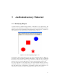
An Introductory Tutorial
3.1 Identifying Shapes . . . . . . . . . . . . .
3.1.1 Divide the Image Into Basic Objects
3.1.2 Identifying the Background . . . .
3.1.3 Shapes and Their Attributes . . . .
3.1.4 The Complete Rule Set . . . . . . .
.
.
.
.
.
.
.
.
.
.
.
.
.
.
.
.
.
.
.
.
.
.
.
.
.
.
.
.
.
.
.
.
.
.
.
.
.
.
.
.
.
.
.
.
.
.
.
.
.
.
.
.
.
.
.
.
.
.
.
.
.
.
.
.
.
.
.
.
.
.
29
29
30
30
32
33
.
.
.
.
.
.
.
.
.
.
.
.
.
.
.
.
.
.
.
.
.
.
.
.
.
.
.
.
.
.
.
.
Basic Rule Set Editing
35
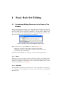
4.1 Creating and Editing Processes in the Process Tree Window . . . . . . . 35
4.1.1 Name . . . . . . . . . . . . . . . . . . . . . . . . . . . . . . . . 35
iii
iv
Developer XD 2.0.4
4.2
4.3
4.4
4.5
5
4.1.2 Algorithm . . . . . . . . . . . . . . . . . . . . . . . .
4.1.3 Image Object Domain . . . . . . . . . . . . . . . . .
4.1.4 Algorithm Parameters . . . . . . . . . . . . . . . . .
Adding a Process . . . . . . . . . . . . . . . . . . . . . . . .
4.2.1 Selecting and Configuring an Image Object Domain .
4.2.2 Adding an Algorithm . . . . . . . . . . . . . . . . . .
4.2.3 Loops & Cycles . . . . . . . . . . . . . . . . . . . .
4.2.4 Executing a Process . . . . . . . . . . . . . . . . . .
4.2.5 Executing a Process on a Selected Object . . . . . . .
4.2.6 Parent and Child Processes . . . . . . . . . . . . . . .
4.2.7 Editing a Rule Set . . . . . . . . . . . . . . . . . . .
4.2.8 Undoing Edits . . . . . . . . . . . . . . . . . . . . .
4.2.9 Deleting a Process or Rule Set . . . . . . . . . . . . .
4.2.10 Editing Using Drag and Drop . . . . . . . . . . . . .
Creating Image Objects Through Segmentation . . . . . . . .
4.3.1 Top-down Segmentation . . . . . . . . . . . . . . . .
4.3.2 Bottom-up Segmentation . . . . . . . . . . . . . . . .
4.3.3 Segmentation by Reshaping Algorithms . . . . . . . .
Object Levels and Segmentation . . . . . . . . . . . . . . . .
4.4.1 About Hierarchical Image Object Levels . . . . . . . .
4.4.2 Creating an Image Object Level . . . . . . . . . . . .
4.4.3 Creating Object Levels With Segmentation Algorithms
4.4.4 Duplicating an Image Object Level . . . . . . . . . .
4.4.5 Editing an Image Object Level or Level Variable . . .
4.4.6 Deleting an Image Object Level . . . . . . . . . . . .
Getting Information on Image Objects . . . . . . . . . . . . .
4.5.1 The Image Object Information Window . . . . . . . .
4.5.2 The Feature View Window . . . . . . . . . . . . . . .
4.5.3 Editing the Feature Distance . . . . . . . . . . . . . .
4.5.4 Comparing Objects Using the Image Object Table . .
4.5.5 Comparing Features Using the 2D Scatter Plot . . . .
4.5.6 Comparing Features Using the 2D Feature Space Plot .
4.5.7 Using Metadata and Features . . . . . . . . . . . . . .
Projects and Workspaces
5.1 Creating a Simple Project . . . . . . . . . . . . . .
5.2 Creating a Project with Predefined Settings . . . .
5.2.1 File Formats . . . . . . . . . . . . . . . .
5.2.2 The Create Project Dialog Box . . . . . . .
5.2.3 Editing Multidimensional Map Parameters
5.2.4 Assigning No-Data Values . . . . . . . . .
5.2.5 Importing Image Layers of Different Scales
5.2.6 Geocoding . . . . . . . . . . . . . . . . .
5.2.7 Multisource Data Fusion . . . . . . . . . .
5.3 Creating, Saving and Loading Workspaces . . . . .
5.3.1 Opening and Creating New Workspaces . .
5.3.2 Importing Scenes into a Workspace . . . .
5.3.3 Importing Images with Annotations . . . .
5.3.4 Configuring the Workspace Display . . . .
5.4 Managing Data in Plate View . . . . . . . . . . .
5.4.1 Navigating Through a Plate . . . . . . . .
27 September 2012
User Guide
.
.
.
.
.
.
.
.
.
.
.
.
.
.
.
.
.
.
.
.
.
.
.
.
.
.
.
.
.
.
.
.
.
.
.
.
.
.
.
.
.
.
.
.
.
.
.
.
.
.
.
.
.
.
.
.
.
.
.
.
.
.
.
.
.
.
.
.
.
.
.
.
.
.
.
.
.
.
.
.
.
.
.
.
.
.
.
.
.
.
.
.
.
.
.
.
.
.
.
.
.
.
.
.
.
.
.
.
.
.
.
.
.
.
.
.
.
.
.
.
.
.
.
.
.
.
.
.
.
.
.
.
.
.
.
.
.
.
.
.
.
.
.
.
.
.
.
.
.
.
.
.
.
.
.
.
.
.
.
.
.
.
.
.
.
.
.
.
.
.
.
.
.
.
.
.
.
.
.
.
.
.
.
.
.
.
.
.
.
.
.
.
.
.
.
.
.
.
.
.
.
.
.
.
.
.
.
.
.
.
.
.
.
.
.
.
.
.
.
.
.
.
.
.
.
.
.
.
.
.
.
.
.
.
.
.
.
.
.
.
.
.
.
.
.
.
.
.
.
.
.
.
.
.
.
.
.
.
.
.
.
.
.
.
.
.
.
.
.
.
.
.
.
.
.
.
.
.
.
.
.
.
.
.
.
.
.
.
.
.
.
.
.
.
35
36
36
36
36
38
39
39
39
40
40
40
41
41
42
42
44
45
47
47
47
48
49
49
50
51
51
52
57
59
59
61
62
.
.
.
.
.
.
.
.
.
.
.
.
.
.
.
.
.
.
.
.
.
.
.
.
.
.
.
.
.
.
.
.
.
.
.
.
.
.
.
.
.
.
.
.
.
.
.
.
.
.
.
.
.
.
.
.
.
.
.
.
.
.
.
.
.
.
.
.
.
.
.
.
.
.
.
.
.
.
.
.
.
.
.
.
.
.
.
.
.
.
.
.
.
.
.
.
65
65
66
66
67
68
69
71
71
72
73
74
75
78
78
79
80
CONTENTS
5.4.2
5.4.3
5.4.4
5.4.5
5.4.6
v
Selecting a Single Well
Select Multiple Wells
Define Plate Layout . .
Save Plate Layout . . .
Load Plate Layout . .
.
.
.
.
.
.
.
.
.
.
.
.
.
.
.
.
.
.
.
.
.
.
.
.
.
.
.
.
.
.
.
.
.
.
.
.
.
.
.
.
.
.
.
.
.
.
.
.
.
.
.
.
.
.
.
.
.
.
.
.
.
.
.
.
.
.
.
.
.
.
.
.
.
.
.
.
.
.
.
.
.
.
.
.
.
.
.
.
.
.
.
.
.
.
.
.
.
.
.
.
.
.
.
.
.
.
.
.
.
.
.
.
.
.
81
81
81
82
82
6
About Classification
83
6.1 Key Classification Concepts . . . . . . . . . . . . . . . . . . . . . . . . 83
6.1.1 Assigning Classes . . . . . . . . . . . . . . . . . . . . . . . . . 83
6.1.2 Class Descriptions and Hierarchies . . . . . . . . . . . . . . . . 83
6.1.3 The Edit Classification Filter . . . . . . . . . . . . . . . . . . . . 88
6.2 Classification Algorithms . . . . . . . . . . . . . . . . . . . . . . . . . . 89
6.2.1 The Assign Class Algorithm . . . . . . . . . . . . . . . . . . . . 89
6.2.2 The Classification Algorithm . . . . . . . . . . . . . . . . . . . . 89
6.2.3 The Hierarchical Classification Algorithm . . . . . . . . . . . . . 90
6.2.4 Advanced Classification Algorithms . . . . . . . . . . . . . . . . 91
6.3 Thresholds . . . . . . . . . . . . . . . . . . . . . . . . . . . . . . . . . . 92
6.3.1 Using Thresholds with Class Descriptions . . . . . . . . . . . . . 92
6.3.2 About the Class Description . . . . . . . . . . . . . . . . . . . . 92
6.3.3 Using Membership Functions for Classification . . . . . . . . . . 93
6.3.4 Evaluation Classes . . . . . . . . . . . . . . . . . . . . . . . . . 97
6.4 Supervised Classification . . . . . . . . . . . . . . . . . . . . . . . . . . 99
6.4.1 Nearest Neighbor Classification . . . . . . . . . . . . . . . . . . 99
6.4.2 Working with the Sample Editor . . . . . . . . . . . . . . . . . . 106
6.4.3 Training and Test Area Masks . . . . . . . . . . . . . . . . . . . 111
6.4.4 The Edit Conversion Table . . . . . . . . . . . . . . . . . . . . . 113
6.4.5 Creating Samples Based on a Shapefile . . . . . . . . . . . . . . 114
6.4.6 Selecting Samples with the Sample Brush . . . . . . . . . . . . . 115
6.4.7 Setting the Nearest Neighbor Function Slope . . . . . . . . . . . 116
6.4.8 Using Class-Related Features in a Nearest Neighbor Feature Space 116
7
Advanced Rule Set Concepts
7.1 Units, Scales and Co-ordinate Systems . . . . . . . . . . . . . . . . . . .
7.2 Thematic Layers and Thematic Objects . . . . . . . . . . . . . . . . . .
7.2.1 Importing, Editing and Deleting Thematic Layers . . . . . . . . .
7.2.2 Displaying a Thematic Layer . . . . . . . . . . . . . . . . . . . .
7.2.3 The Thematic Layer Attribute Table . . . . . . . . . . . . . . . .
7.2.4 Manually Editing Thematic Vector Objects . . . . . . . . . . . .
7.2.5 Using a Thematic Layer for Segmentation . . . . . . . . . . . . .
7.3 Variables in Rule Sets . . . . . . . . . . . . . . . . . . . . . . . . . . . .
7.3.1 About Variables . . . . . . . . . . . . . . . . . . . . . . . . . . .
7.3.2 Creating a Variable . . . . . . . . . . . . . . . . . . . . . . . . .
7.3.3 Saving Variables as Parameter Sets . . . . . . . . . . . . . . . .
7.4 Arrays . . . . . . . . . . . . . . . . . . . . . . . . . . . . . . . . . . . .
7.4.1 Creating Arrays . . . . . . . . . . . . . . . . . . . . . . . . . . .
7.4.2 Order of Array Items . . . . . . . . . . . . . . . . . . . . . . . .
7.4.3 Using Arrays in Rule Sets . . . . . . . . . . . . . . . . . . . . .
7.5 Image Objects and Their Relationships . . . . . . . . . . . . . . . . . . .
7.5.1 Implementing Child Domains via the Execute Child Process Algorithm . . . . . . . . . . . . . . . . . . . . . . . . . . . . . . .
7.5.2 Child Domains and Parent Processes . . . . . . . . . . . . . . . .
User Guide
119
119
120
120
121
121
122
128
129
129
130
133
135
135
136
136
136
136
137
27 September 2012
vi
Developer XD 2.0.4
7.6
7.7
7.8
7.9
7.10
7.11
7.12
7.13
8
Tutorial: Using Process-Related Features for Advanced Local Processing
Customized Features . . . . . . . . . . . . . . . . . . . . . . . . . . . .
7.7.1 Creating Customized Features . . . . . . . . . . . . . . . . . . .
7.7.2 Arithmetic Customized Features . . . . . . . . . . . . . . . . . .
7.7.3 Relational Customized Features . . . . . . . . . . . . . . . . . .
7.7.4 Saving and Loading Customized Features . . . . . . . . . . . . .
7.7.5 Finding Customized Features . . . . . . . . . . . . . . . . . . .
7.7.6 Defining Feature Groups . . . . . . . . . . . . . . . . . . . . . .
Customized Algorithms . . . . . . . . . . . . . . . . . . . . . . . . . . .
7.8.1 Dependencies and Scope Consistency Rules . . . . . . . . . . . .
7.8.2 Handling of References to Local Items During Runtime . . . . .
7.8.3 Domain Handling in Customized Algorithms . . . . . . . . . . .
7.8.4 Creating a Customized Algorithm . . . . . . . . . . . . . . . . .
7.8.5 Using Customized Algorithms . . . . . . . . . . . . . . . . . . .
7.8.6 Modifying a Customized Algorithm . . . . . . . . . . . . . . . .
7.8.7 Executing a Customized Algorithm for Testing . . . . . . . . . .
7.8.8 Deleting a Customized Algorithm . . . . . . . . . . . . . . . . .
7.8.9 Using a Customized Algorithm in Another Rule Set . . . . . . .
Maps . . . . . . . . . . . . . . . . . . . . . . . . . . . . . . . . . . . .
7.9.1 The Maps Concept . . . . . . . . . . . . . . . . . . . . . . . . .
7.9.2 Adding a Map to a Project to Create Multi-Project Maps . . . . .
7.9.3 Copying a Map for Multi-Scale Analysis . . . . . . . . . . . . .
7.9.4 Editing Map Properties . . . . . . . . . . . . . . . . . . . . . . .
7.9.5 Displaying Maps . . . . . . . . . . . . . . . . . . . . . . . . . .
7.9.6 Synchronizing Maps . . . . . . . . . . . . . . . . . . . . . . . .
7.9.7 Saving and Deleting Maps . . . . . . . . . . . . . . . . . . . . .
7.9.8 Working with Multiple Maps . . . . . . . . . . . . . . . . . . . .
Workspace Automation . . . . . . . . . . . . . . . . . . . . . . . . . . .
7.10.1 Overview . . . . . . . . . . . . . . . . . . . . . . . . . . . . . .
7.10.2 Manually Creating Copies and Tiles . . . . . . . . . . . . . . . .
7.10.3 Manually Stitch Scene Subsets and Tiles . . . . . . . . . . . . .
7.10.4 Processing Sub-Scenes with Subroutines . . . . . . . . . . . . .
7.10.5 Multi-Scale Workflows . . . . . . . . . . . . . . . . . . . . . . .
Object Links . . . . . . . . . . . . . . . . . . . . . . . . . . . . . . . . .
7.11.1 About Image Object Links . . . . . . . . . . . . . . . . . . . . .
7.11.2 Image Objects and their Relationships . . . . . . . . . . . . . . .
7.11.3 Creating and Saving Image Object Links . . . . . . . . . . . . .
Polygons and Skeletons . . . . . . . . . . . . . . . . . . . . . . . . . . .
7.12.1 Viewing Polygons . . . . . . . . . . . . . . . . . . . . . . . . .
7.12.2 Viewing Skeletons . . . . . . . . . . . . . . . . . . . . . . . . .
Encrypting and Decrypting Rule Sets . . . . . . . . . . . . . . . . . . . .
Additional Development Tools
8.1 The Find and Replace Bar . . . . . . . . . . . .
8.1.1 Find and Replace Modifiers . . . . . . .
8.2 Rule Set Documentation . . . . . . . . . . . . .
8.2.1 Adding Comments . . . . . . . . . . . .
8.2.2 The Rule Set Documentation Window . .
8.3 Process Paths . . . . . . . . . . . . . . . . . . .
8.4 Improving Performance with the Process Profiler
8.5 Snippets . . . . . . . . . . . . . . . . . . . . . .
27 September 2012
User Guide
.
.
.
.
.
.
.
.
.
.
.
.
.
.
.
.
.
.
.
.
.
.
.
.
.
.
.
.
.
.
.
.
.
.
.
.
.
.
.
.
.
.
.
.
.
.
.
.
.
.
.
.
.
.
.
.
.
.
.
.
.
.
.
.
.
.
.
.
.
.
.
.
.
.
.
.
.
.
.
.
.
.
.
.
.
.
.
.
.
.
.
.
.
.
.
.
.
.
.
.
.
.
.
.
141
143
145
145
146
150
150
150
151
151
152
153
153
156
156
157
157
157
158
158
159
159
160
160
160
161
161
162
162
164
165
165
167
172
172
173
173
175
175
177
178
179
179
180
180
180
181
181
181
182
CONTENTS
8.5.1
9
vii
Snippets Options . . . . . . . . . . . . . . . . . . . . . . . . . . 183
Automating Data Analysis
9.1 Loading and Managing Data . . . . . . . . . . . .
9.1.1 Projects and Workspaces . . . . . . . . . .
9.1.2 Data Import . . . . . . . . . . . . . . . . .
9.1.3 Collecting Statistical Results of Subscenes
9.1.4 Executing Rule Sets with Subroutines . . .
9.1.5 Tutorials . . . . . . . . . . . . . . . . . .
9.2 Batch Processing . . . . . . . . . . . . . . . . . .
9.2.1 Submitting Batch Jobs to a Server . . . . .
9.2.2 Tiling and Stitching . . . . . . . . . . . . .
9.2.3 Interactive Workflows . . . . . . . . . . .
9.3 Exporting Data . . . . . . . . . . . . . . . . . . .
9.3.1 Automated Data Export . . . . . . . . . .
9.3.2 Reporting Data on a Single Project . . . . .
9.3.3 Exporting the Contents of a Window . . . .
.
.
.
.
.
.
.
.
.
.
.
.
.
.
.
.
.
.
.
.
.
.
.
.
.
.
.
.
.
.
.
.
.
.
.
.
.
.
.
.
.
.
.
.
.
.
.
.
.
.
.
.
.
.
.
.
.
.
.
.
.
.
.
.
.
.
.
.
.
.
.
.
.
.
.
.
.
.
.
.
.
.
.
.
.
.
.
.
.
.
.
.
.
.
.
.
.
.
.
.
.
.
.
.
.
.
.
.
.
.
.
.
.
.
.
.
.
.
.
.
.
.
.
.
.
.
.
.
.
.
.
.
.
.
.
.
.
.
.
.
.
.
.
.
.
.
.
.
.
.
.
.
.
.
185
185
185
188
196
196
196
198
198
201
203
203
203
203
208
10 Rule Sets for Definiens Architect XD
10.1 Action Libraries . . . . . . . . . . . . . . . . . . . . .
10.1.1 Creating User Parameters . . . . . . . . . . .
10.1.2 Creating a Quick Test Button . . . . . . . . . .
10.1.3 Maintaining Rule Sets for Actions . . . . . . .
10.1.4 Workspace Automation . . . . . . . . . . . . .
10.1.5 Creating a New Action Library . . . . . . . . .
10.1.6 Assembling and Editing an Action Library . .
10.1.7 Updating a Solution while Developing Actions
10.1.8 Building an Analysis Solution . . . . . . . . .
10.1.9 Editing Widgets for Action Properties . . . . .
10.1.10 Exporting Action Definition to File . . . . . .
.
.
.
.
.
.
.
.
.
.
.
.
.
.
.
.
.
.
.
.
.
.
.
.
.
.
.
.
.
.
.
.
.
.
.
.
.
.
.
.
.
.
.
.
.
.
.
.
.
.
.
.
.
.
.
.
.
.
.
.
.
.
.
.
.
.
.
.
.
.
.
.
.
.
.
.
.
.
.
.
.
.
.
.
.
.
.
.
.
.
.
.
.
.
.
.
.
.
.
.
.
.
.
.
.
.
.
.
.
.
211
211
211
212
212
213
213
213
217
218
225
226
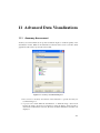
11 Advanced Data Visualizations
11.1 Accuracy Assessment . . . . . . . . . . .
11.1.1 Classification Stability . . . . . .
11.1.2 Error Matrices . . . . . . . . . .
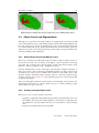
11.2 Tissue . . . . . . . . . . . . . . . . . . .
11.2.1 The Heat Map . . . . . . . . . .
11.3 TMA Grid View . . . . . . . . . . . . . .
11.3.1 Defining the Grid Layout . . . . .
11.3.2 Matching Cores to the Grid . . . .
11.3.3 Changing the Grid After Matching
11.3.4 Editing Cores . . . . . . . . . . .
11.4 Cellenger . . . . . . . . . . . . . . . . .
11.4.1 Plate View . . . . . . . . . . . .
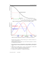
11.4.2 Creating Dose-Response Curves .
11.5 Accept and Reject Results . . . . . . . .
.
.
.
.
.
.
.
.
.
.
.
.
.
.
.
.
.
.
.
.
.
.
.
.
.
.
.
.
.
.
.
.
.
.
.
.
.
.
.
.
.
.
.
.
.
.
.
.
.
.
.
.
.
.
.
.
.
.
.
.
.
.
.
.
.
.
.
.
.
.
.
.
.
.
.
.
.
.
.
.
.
.
.
.
.
.
.
.
.
.
.
.
.
.
.
.
.
.
.
.
.
.
.
.
.
.
.
.
.
.
.
.
.
.
.
.
.
.
.
.
.
.
.
.
.
.
.
.
.
.
.
.
.
.
.
.
.
.
.
.
227
227
228
229
230
230
233
233
234
236
237
238
238
242
246
.
.
.
.
.
.
.
.
.
.
.
.
.
.
.
.
.
.
.
.
.
.
.
.
.
.
.
.
.
.
.
.
.
.
.
.
.
.
.
.
.
.
.
.
.
.
.
.
.
.
.
.
.
.
.
.
.
.
.
.
.
.
.
.
.
.
.
.
.
.
.
.
.
.
.
.
.
.
.
.
.
.
.
.
.
.
.
.
.
.
.
.
.
.
.
.
.
.
.
.
.
.
.
.
.
.
.
.
.
.
.
.
12 Options
247
13 Aperio Spectrum Database Integration
253
13.1 Creating a Developer XD Workspace from the Aperio Spectrum Database 253
User Guide
27 September 2012
viii
Developer XD 2.0.4
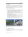
Acknowledgments
27 September 2012
255
User Guide
1
Key Concepts
This chapter will introduce some terminology that you will encounter.
1.1
Image Layer
In Definiens Developer XD 2.0.4, an image layer is the most basic level of information
contained in a raster image. All images contain at least one image layer.
A grayscale image is an example of an image with one layer. whereas the most common
single layers are the red, green and blue (RGB) layers that go together to create a color
image. In addition, image layers can contain information such as the intensity values
of biomarkers used in life sciences or the near-infrared (NIR) data contained in remote
sensing images. Image layers can also contain a range of other information, such as
geographical elevation models.
Definiens Developer XD 2.0.4 allows the import of these image raster layers. It also
supports what are known as thematic raster layers, which can contain qualitative and
categorical information about an area (an example is a layer that acts as a mask to identify
a particular region).
1.2
Image Data Set
Definiens software handles two-dimensional images and data sets of multidimensional,
visual representations:
• A 2D image is set of raster image data representing a two-dimensional image. Its
co-ordinates are (x, y). Its elementary unit is a pixel.
• A 3D data set is a set of layered 2D images, called slices. A 3D data set consists
of a stack of slices, representing a three-dimensional space. Its co-ordinates are
(x, y, z). Its elementary unit is a voxel.
• A 4D data set is a temporal sequence of 3D data sets. A 4D data set consists of
a series of frames, each frame consisting of a 3D data set. Its co-ordinates are
(x, y, z,t). Its elementary unit is a voxel series.
• A time series data set is a sequence of 2D images, commonly called film. A time
series data set consists of a series of frames where each frame is a 2D image. Its
co-ordinates are (x, y,t). Its elementary unit is a pixel series.
1
2
1.3
Developer XD 2.0.4
Segmentation and classification
The first step of a Definiens image analysis is to cut the image into pieces, which serve as
building blocks for further analysis – this step is called segmentation and there is a choice
of several algorithms to do this.
The next step is to label these objects according to their attributes, such as shape, color
and relative position to other objects. This is typically followed by another segmentation
step to yield more functional objects. This cycle is repeated as often as necessary and the
hierarchies created by these steps are described in the next section.
1.4
1.4.1
Image Objects, Hierarchies and Domains
Image Objects
An image object is a group of pixels in a map. Each object represents a definite space
within a scene and objects can provide information about this space. The first image
objects are typically produced by an initial segmentation.
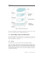
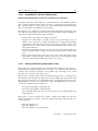
1.4.2
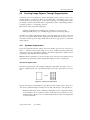
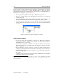
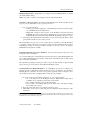
Image Object Hierarchy
This is a data structure that incorporates image analysis results, which have been extracted
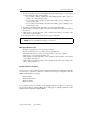
from a scene. The concept is illustrated in figure 1.1 on the facing page.
It is important to distinguish between image object levels and image layers. Image layers
represent data that already exists in the image when it is first imported. Image object
levels store image objects, which are representative of this data.
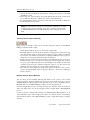
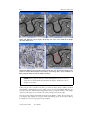
The scene below is represented at the pixel level and is an image of a cell. Each level has
a super-level above it, where multiple objects may become assigned to single classes –
for example, the cell level is the super-level containing the cell body and nucleus, whose
objects comprise it.
Every image object is networked in a manner that each image object knows its context –
who its neighbors are, which levels and objects (superobjects) are above it and which are
below it (sub-objects). No image object may have more than one superobject, but it can
have multiple sub-objects.
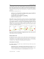
1.4.3
Image Object Domain
The image object domain describes the scope of a process; in other words, which image
objects (or pixels) an algorithm is applied to. For example, an image object domain is
created when you select objects based on their size.
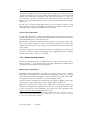
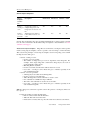
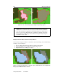
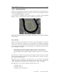
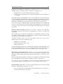
A segmentation-classification-segmentation cycle is illustrated in figure 1.2 on page 4.
The square is segmented into four and the regions are classified into A and B. Region B
then undergoes further segmentation. The relevant image object domain is listed underneath the corresponding algorithm.
27 September 2012
User Guide
Key Concepts
3
Figure 1.1. The hierarchy of image objects
You can also define image object domains by their relations to image objects of parent
processes, for example, sub-objects or neighboring image objects.
1.5
Scenes, Maps, Projects and Workspaces
The organizational hierarchy in Definiens software is – in ascending order – scenes, maps,
projects and workspaces. As this terminology is used extensively in this guide, it is
important to familiarize yourself with it.
1.5.1
Scenes
On a practical level, a scene is the most basic level in the Definiens hierarchy.
A scene is essentially a digital image along with some associated information. For example, in its most basic form, a scene could be a JPEG image from a digital camera
with the associated metadata (such as size, resolution, camera model and date) that the
camera software adds to the image. At the other end of the spectrum, it could be a
four-dimensional medical image set, with an associated file containing a thematic layer
containing histological data.
User Guide
27 September 2012
4
Developer XD 2.0.4
Figure 1.2. Different image object domains of a process sequence
1.5.2
Maps and Projects
The image file and the associated data within a scene can be independent of Definiens
software (although this is not always true). However, Developer XD will import all of
this information and associated files, which you can then save to a Definiens format; the
most basic one being aa Definiens project (which has a .dpr extension). A dpr file is
separate to the image and – although they are linked objects – does not alter it.
What can be slightly confusing in the beginning is that Developer XD creates another
hierarchical level between a scene and a project – a map. Creating a project will always
create a single map by default, called the main map – visually, what is referred to as the
main map is identical to the original image and cannot be deleted.
Maps only really become useful when there are more than one of them, because a single
project can contain several maps. A practical example is a second map that contains a
portion of the original image at a lower resolution. When the image within that map is
analyzed, the analysis and information from that scene can be applied to the more detailed
original.
1.5.3
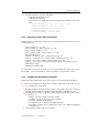
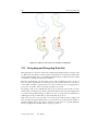
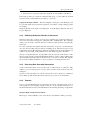
Workspaces
Workspaces are at the top of the hierarchical tree and are essentially containers for
projects, allowing you to bundle several of them together. They are especially useful
for handling complex image analysis tasks where information needs to be shared. The
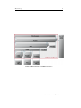
Definiens hierarchy is represented in figure 1.3 on the facing page.
27 September 2012
User Guide
Key Concepts
5
Figure 1.3. Data structure of a Definiens workspace
User Guide
27 September 2012
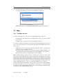
2
Starting Developer
Definiens clients share portals with predefined user interfaces. A portal provides a selection of tools and user interface elements typically used for image analysis within an
industry or science domain. However, most tools and user interface elements that are
hidden by default are still available.
2.1
The Developer XD Portal
The following portals are available:
• Cell – recommended for cell-based image analysis. Standard portal for Definiens
Cellenger application
• Tissue – recommended for tissue-based image analysis. Standard portal for
Definiens TissueMap application
• TMA – recommended for the analysis of tissue micro arrays. Standard portal for
Definiens TMA application
• Life – standard portal for the life sciences domain
We recommend you do not use the Cell, Tissue or TMA portals for rule-set development,
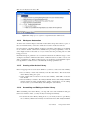
as this will create unwanted layers. Users should use the Life portal in this case.
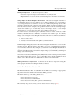
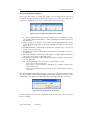
Open Definiens Developer XD 2.0.4 from the Windows Start menu and select a portal.
Click any portal item to stop automatic opening. If you do not click a portal within three
seconds, the most recently used portal will start. To start a different portal, close the client
and start again.
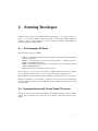
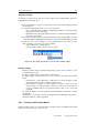
2.2
Developer Portal with Tissue Studio™ License
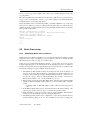
Customers who have also purchased Definiens Tissue Studio™ licenses will see further
start-up options relating to this product. For more details, see the Tissue Studio™ User
Guide.
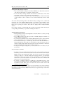
7
8
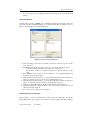
Developer XD 2.0.4
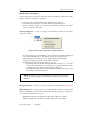
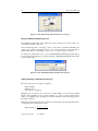
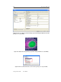
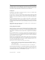
Figure 2.1. Start-up options for Definiens Developer XD 2.0.4
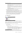
Figure 2.2. Portals available for Developer Customers with Tissue Studio™ licenses
27 September 2012
User Guide
Starting Developer
9
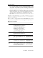
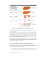
Portal
Application
Tissue Studio
Brightfield whole tissue analysis
Tissue Studio (TMA)
Brightfield tissue micro array analysis
Tissue Studio IF
Fluorescence whole tissue analysis
Tissue Studio IF (TMA) Fluorescence tissue micro array analysis
2.3
Starting Multiple Definiens Clients
You can start and work on multiple Developer XD clients simultaneously; this is helpful
if you want to open more than one project at the same time. However, you cannot interact
directly between two active applications, as they are running independently – for example,
dragging and dropping between windows is not possible.
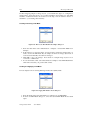
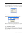
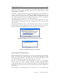
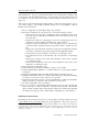
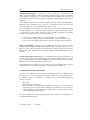
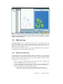
2.4
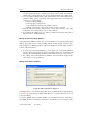
The Develop Rule Sets View
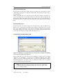
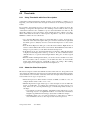
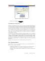
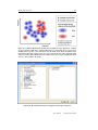
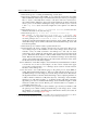
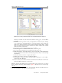
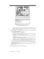
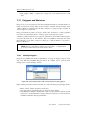
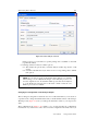
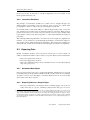
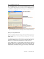
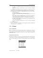
Figure 2.3. The default workspace when a project or image is opened in the application (in
this case the Cell portal)
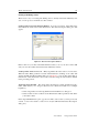
1. The map view displays the image file. Up to four windows can be displayed by selecting Window > Split Vertically and Window > Split Horizontally from the main
menu, allowing you to assign different views of an image to each window. The
User Guide
27 September 2012
10
Developer XD 2.0.4
2.
3.
4.
5.
2.5
2.5.1
image can be enlarged or reduced using the Zoom functions on the main toolbar
(or from the View menu)
The Process Tree: Developer XD uses a cognition language to create ruleware.
These functions are created by writing rule sets in the Process Tree window
Class Hierarchy: Image objects can be assigned to classes by the user, which are
displayed in the Class Hierarchy window. The classes can be grouped in a hierarchical structure, allowing child classes to inherit attributes from parent classes
Image Object Information: This window provides information about the characteristics of image objects
Feature View: In Definiens software, a feature represents information such as measurements, attached data or values. Features may relate to specific objects or apply
globally and available features are listed in the Feature View window.
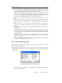
Customizing the Layout
Default Toolbar Buttons
File Toolbar
The File toolbars allow you to load image files, open projects, and open and create new
workspaces.
View Settings Toolbar
These buttons, numbered from one to four, allow you to switch between the four window
layouts. These are Load and Manage Data, Configure Analysis, Review Results and
Develop Rule Sets.
As much of the User Guide centers around writing rule sets – which organize and modify
image analysis algorithms – the view activated by button number four, Develop Rule Sets,
is most commonly used
This group of buttons allows you to select image view options, offering views of layers,
classifications and any features you wish to visualize.
This group is concerned with displaying outlines and borders of image objects, and views
of pixels.
27 September 2012
User Guide
Starting Developer
11
These toolbar buttons allow you to visualize different layers; in grayscale or in RGB.
They also allow you to switch between layers and to mix them.
Zoom Functions Toolbar
This region of the toolbar offers direct selection and the ability to drag an image, along
with several zoom options.
View Navigate Toolbar
The View Navigate folder allows you to delete levels, select maps and navigate the object
hierarchy.
Tools Toolbar
The Tools toolbar allow access to advanced dialog boxes:
The buttons on the Tools toolbar launch the following dialog boxes and toolbars:
•
•
•
•
•
•
•
•
2.5.2
The Manual Editing Toolbar
Manage Customized Features
Manage Variables
Manage Parameter Sets
Undo
Redo
Save Current Project State
Restore Saved Project State
Splitting Windows
There are several ways to customize the layout in Developer XD, allowing you to display
different views of the same image. For example, you may wish to compare the results of
a segmentation alongside the original image.
Selecting Window > Split allows you to split the window into four – horizontally and
vertically – to a size of your choosing. Alternatively, you can select Window > Split
Horizontally or Window > Split Vertically to split the window into two.
There are two more options that give you the choice of synchronizing the displays. Independent View allows you to make changes to the size and position of individual windows
– such as zooming or dragging images – without affecting other windows. Alternatively,
User Guide
27 September 2012
12
Developer XD 2.0.4
selecting Side-by-Side View will apply any changes made in one window to any other
windows.
A final option, Swipe View, displays the entire image into across multiple sections, while
still allowing you to change the view of an individual section
2.5.3
Magnifier
The Magnifier feature lets you view a magnified area of a region of interest in a separate
window. It offers a zoom factor five times greater than the one available in the normal
map view.
To open the Magnifier window, select View > Windows > Magnifier from the main men.
Holding the cursor over any point of the map centers the magnified view in the Magnifier
window. You can release the Magnifier window by dragging it while holding down the
Ctrl key.
2.5.4
Docking
By default, the four commonly used windows – Process Tree, Class Hierarchy, Image
Object Information and Feature View – are displayed on the right-hand side of the
workspace, in the default Develop Rule Set view. The menu item Window > Enable
Docking facilitates this feature.
When you deselect this item, the windows will display independently of each other, allowing you to position and resize them as you wish. This feature may be useful if you
are working across multiple monitors. Another option to undock windows is to drag a
window while pressing the Ctrl key.
You can restore the window layouts to their default positions by selecting View > Restore
Default. Selecting View > Save Current View also allows you to save any changes to the
workspace view you make.
2.5.5
Developer XD Views
View Layer
To view your original image pixels, you will need to click the View Layer button on the
toolbar. Depending on the stage of your analysis, you may also need to select Pixel View
(by clicking the Pixel View or Object Mean View button).
In the View Layer view (figure 2.4), you can also switch between the grayscale and RGB
layers, using the buttons to the right of the View Settings toolbar. To view an image in its
original format (if it is RGB), you may need to press the Mix Three Layers RGB button .
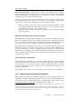
View Classification
Used on its own, View Classification will overlay the colors you manually assign when
classifying objects (these are the classifications visible in the Class Hierarchy window) –
figure 2.5 on the next page shows the same object when displayed in pixel view with all
27 September 2012
User Guide
Starting Developer
13
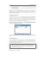
Figure 2.4. Two images displayed using Layer View. The left-hand image is displayed in RGB,
while the right-hand image displays the red layer only
its RGB layers (as outlined in the previous section), against its appearance when View
Classification is selected.
Clicking the Pixel View or Object Mean View button toggles between an opaque overlay
(in Object Mean View) and a semi-transparent overlay (in Pixel View). When in Pixel
View, a button appears at the bottom of the image window – clicking on this button will
display a transparency slider, which allows you to customize the level of transparency.
Figure 2.5. An object for analysis displayed with all layers in Pixel View, next to the same
image in Classification View. The colors in the right-hand image have been assigned by the
user and follow segmentation and identification of image objects
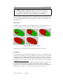
Feature View
The Feature View button may be deactivated when you open a project. It becomes active
when you select a feature in the Feature View window by double-clicking on it.
Image objects are displayed as grayscale according to the feature selected (figure 2.6).
Low feature values are darker, while high values are brighter. If an object is red, it has
not been defined for the evaluation of the chosen feature.
Pixel View or Object Mean View
This button switches between Pixel View and Object Mean View.
Object Mean View creates an average color value of the pixels in each object, displaying
everything as a solid color (figure 2.7). If Classification View is active, the Pixel View
User Guide
27 September 2012
14
Developer XD 2.0.4
Figure 2.6. An image in normal Pixel View compared to the same image in Feature View, with
the Area algorithm selected from the Feature View window
is displayed semi-transparently through the classification. Again, you can customize the
transparency in the same way as outlined in View Classification on page 12.
Figure 2.7. Object displayed in Pixel View, at 50% opacity (left) and 100% opacity (right)
Show or Hide Outlines
The Show or Hide Outlines button allows you to display the borders of image objects
(figure 2.8) that you have created by segmentation and classification. The outline colors
vary depending on the active display mode:
• In View Layer mode, the outline colors are defined in the Edit Highlight Colors
dialog box (View > Display Mode > Edit Highlight Colors)
• In View Classification mode, the outlines take on the colors of the respective classes
Image View or Project Pixel View
Image View or Project Pixel View is a more advanced feature, which allows the comparison of a downsampled scene (assuming you have created one) with the original. Pressing
this button toggles between the two views.
27 September 2012
User Guide
Starting Developer
15
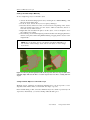
Figure 2.8. Images displayed with visible outlines. The left-hand image is displayed in Layer
View. The right-hand image is displayed with View Classification selected and the outline
colors are based on user classification colors
2.5.6
Image Layer Display
Single Layer Grayscale
Scenes are automatically assigned RGB (red, green and blue) colors by default when
image data with three or more image layers is loaded. Use the Single Layer Grayscale
button on the View Settings toolbar to display the image layers separately in grayscale.
In general, when viewing multilayered scenes, the grayscale mode for image display
provides valuable information. To change from default RGB mode to grayscale mode, go
to the toolbar and press the Single Layer Grayscale button, which will display only the
first image layer in grayscale mode.
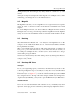
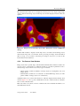
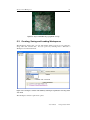
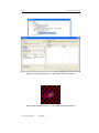
Figure 2.9. Layer 1 single grayscale map view of a sample scene of microtubules. (Image data
courtesy of EMBL Heidelberg.)
Three Layers RGB
Display three layers to see your scene in RGB. By default, layer one is assigned to the red
channel, layer two to green, and layer three to blue. The color of an image area informs
the viewer about the particular image layer, but not its real color. These are additively
mixed to display the image in the map view. You can change these settings in the Edit
Image Layer Mixing dialog box.
User Guide
27 September 2012
16
Developer XD 2.0.4
Show Previous Image Layer
In Grayscale mode, this button displays the previous image layer. The number or name
of the displayed image layer is indicated in the middle of the status bar at the bottom of
the main window.
In Three Layer Mix, the color composition for the image layers changes one image layer
up for each image layer. For example, if layers two, three and four are displayed, the
Show Previous Image Layer Button changes the display to layers one, two and three. If
the first image layer is reached, the previous image layer starts again with the last image
layer.
Show Next Image Layer
In Grayscale mode, this button displays the next image layer down. In Three Layer
Mix, the color composition for the image layers changes one image layer down for each
layer. For example, if layers two, three and four are displayed, the Show Next Image
Layer Button changes the display to layers three, four and five. If the last image layer is
reached, the next image layer begins again with image layer one.
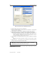
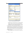
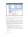
The Edit Image Layer Mixing Dialog Box
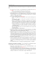
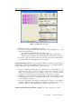
Figure 2.10. Edit Image Layer Mixing dialog box. Changing the layer mixing and equalizing
options affects the display of the image only
You can define the color composition for the visualization of image layers for display
in the map view. In addition, you can choose from different equalizing options. This
enables you to better visualize the image and to recognize the visual structures without
actually changing them. You can also choose to hide layers, which can be very helpful
when investigating image data and results.
NOTE: Changing the image layer mixing only changes the visual display
of the image but not the underlying image data – it has no impact on the
process of image analysis.
27 September 2012
User Guide
Starting Developer
17
When creating a new project, the first three image layers are displayed in red, green and
blue.
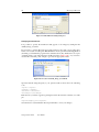
1. To change the layer mixing, open the Edit Image Layer Mixing dialog box (figure 2.10):
• Choose View > Image Layer Mixing from the main menu.
• Double-click in the right pane of the View Settings window.
2. Define the display color of each image layer. For each image layer you can set
the weighting of the red, green and blue channels. Your choices can be displayed
together as additive colors in the map view. Any layer without a dot or a value in
at least one column will not display.
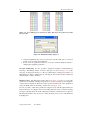
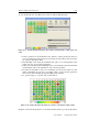
3. Choose a layer mixing preset (see figure 2.11):
• (Clear): All assignments and weighting are removed from the Image Layer
table
• One Layer Gray displays one image layer in grayscale mode with the red,
green and blue together
• False Color (Hot Metal) is recommended for single image layers with large
intensity ranges to display in a color range from black over red to white. Use
this preset for image data created with positron emission tomography (PET)
• False Color (Rainbow) is recommended for single image layers to display a
visualization in rainbow colors. Here, the regular color range is converted to a
color range between blue for darker pixel intensity values and red for brighter
pixel intensity values
• Three Layer Mix displays layer one in the red channel, layer two in green and
layer three in blue
• Six Layer Mix displays additional layers
4. Change these settings to your preferred options with the Shift button or by clicking
in the respective R, G or B cell. One layer can be displayed in more than one color,
and more than one layer can be displayed in the same color.
5. Individual weights can be assigned to each layer. Clear the No Layer Weights
check-box and click a color for each layer. Left-clicking increases the layer’s color
weight while right-clicking decreases it. The Auto Update checkbox refreshes the
view with each change of the layer mixing settings. Clear this check box to show
the new settings after clicking OK. With the Auto Update check box cleared, the
Preview button becomes active.
6. Compare the available image equalization methods and choose one that gives you
the best visualization of the objects of interest. Equalization settings are stored in
the workspace and applied to all projects within the workspace, or are stored within
a separate project. In the Options dialog box you can define a default equalization
setting.
7. Click the Parameter button to changing the equalizing parameters, if available.
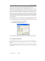
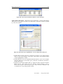
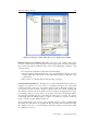
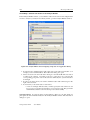
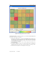
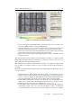
Editing Image Layer Mixing for Thumbnails You can change the way thumbnails display
in the Heat Map window and in the Thumbnail Views of the workspace:
1. Right-click on the Heat Map window or go to View > Thumbnail Settings to open
the Thumbnail Settings dialog box (figure 2.12).
2. Choose among different layer mixes in the Layer Mixing drop-down list. The One
Layer Gray preset displays a layer in grayscale mode with the red, green and blue
together. The three layer mix displays layer 1 in the red channel, layer 2 in green
and layer 3 in blue. Choose six layer mix to display additional layers.
User Guide
27 September 2012
18
Developer XD 2.0.4
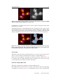
Figure 2.11. Layer Mixing presets (from left to right): One-Layer Gray, Three-Layer Mix,
Six-Layer Mix
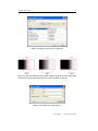
Figure 2.12. Thumbnail Settings dialog box
3. Using the Equalizing drop-down box and select a method that gives you the best
display of the objects in the thumbnails.
4. If you select an equalization method you can also click the Parameter button to
changing the equalizing parameters.
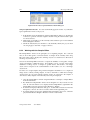
It is also possible to change the visibility of individual layers
and maps. The Manage Aliases for Layers dialog box is shown in figure 2.13 on the
next page. To display the dialog, go to Process > Edit Aliases > Image Layer Aliases (or
Thematic Layer Aliases). Hide a layer by selecting the alias in the left-hand column and
unchecking the ‘visible’ checkbox.
The Layer Visibility Flag
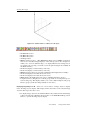
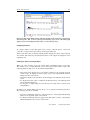
The Window Leveling dialog box (figure 2.15) lets you control the
parameters for manually adjusting image levels on-screen. Leveling sets the brightness
of pixels that are displayed. The Center value specifies the mid-point of the equalization
range; the Width value sets the limits on either side of it (figure 2.14).
Window Leveling
It is also possible to adjust these parameters using the mouse with the right-hand mouse
button held down – moving the mouse horizontally adjusts the center of window leveling;
moving it vertically adjusts the width. (This function must be enabled in Tools > Options.)
The Predefined Values drop-down box contains medical presets for use with Definiens
Lung Expert™.
27 September 2012
User Guide
Starting Developer
19
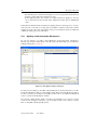
Figure 2.13. Manage Aliases for Layers dialog box
Figure 2.14. Window leveling. On a black-white gradient, adjusting the center value defines
the mid-point of the gradient. The width value specifies the limits on each side
Figure 2.15. The Window Leveling dialog box
User Guide
27 September 2012
20
Developer XD 2.0.4
Image Equalization
Image equalization is performed after all image layers are mixed into a raw RGB (red,
green, blue) image. If, as is usual, one image layer is assigned to each color, the effect is
the same as applying equalization to the individual raw layer gray value images. On the
other hand, if more than one image layer is assigned to one screen color (red, green or
blue), image equalization leads to higher quality results if it is performed after all image
layers are mixed into a raw RGB image.
There are several modes for image equalization:
• None: No equalization allows you to see the scene as it is, which can be helpful at
the beginning of rule set development when looking for an approach. The output
from the image layer mixing is displayed without further modification
• Linear Equalization with 1.00% is the default for new scenes. Commonly it displays images with a higher contrast than without image equalization
• Standard Deviation Equalization has a default parameter of 3.0 and renders a display similar to the Linear equalization. Use a parameter around 1.0 for an exclusion
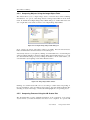
of dark and bright outliers
• Gamma Correction Equalization is used to improve the contrast of dark or bright
areas by spreading the corresponding gray values
• Histogram Equalization is well-suited for Landsat images but can lead to substantial over-stretching on many normal images. It can be helpful in cases where you
want to display dark areas with more contrast
• Manual Image Layer Equalization enables you to control equalization in detail. For
each image layer, you can set the equalization method. In addition, you can define
the input range by setting minimum and maximum values.
Compare the following displays of the same scene:
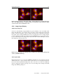
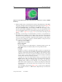
Figure 2.16. Left: Three layer mix (red, green, blue) with Gamma correction (0.50). Right:
One layer mix with linear equalizing (1.00%)
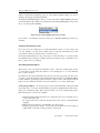
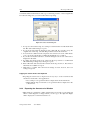
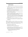
2.5.7
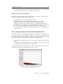
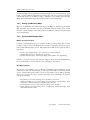
Adding Text to an Image
In some instances, it is desirable to display text over an image – for example, patients’
names on MRI and CT scans. In addition, text can be incorporated into a digital image if
it is exported as part of a rule set.
27 September 2012
User Guide
Starting Developer
21
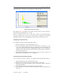
Figure 2.17. Left: Three layer mix (red, green, blue) without equalizing. Right: Six-layer mix
with Histogram equalization. (Image data courtesy of the Ministry of Environmental Affairs
of Sachsen-Anhalt, Germany.)
Figure 2.18. MRI scan with text display
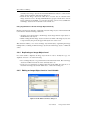
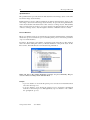
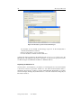
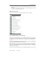
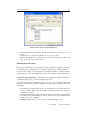
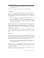
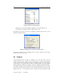
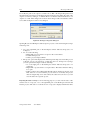
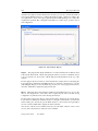
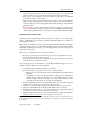
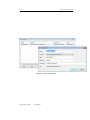
To add text, double click on the image in the corner of Map View (not the image itself)
where you want to add the text, which causes the appropriate Edit Text Settings window
to launch (figure 2.19).
The buttons on the right allow you to insert the fields for map name, slice position and any
values you wish to display. The drop-down boxes at the bottom let you edit the attributes
of the text. Note that the two-left hand corners always display left-justified text and the
right hand corners show right-justified text.
Text rendering settings can be saved or loaded using the Save and Load buttons; these
settings are saved in files with the extension .dtrs. If you wish to export an image as
part of a rule set with the text displayed, it is necessary to use the Export Current View
algorithm with the Save Current View Settings parameter. Image object information is
not exported.
If a project contains multiple slices, all slices will be labelled.
User Guide
27 September 2012
22
Developer XD 2.0.4
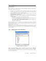
Figure 2.19. The Edit Text Settings dialog box
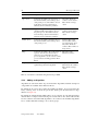
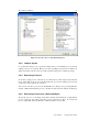
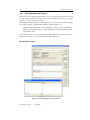
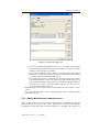
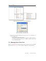
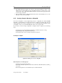
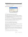
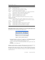
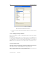
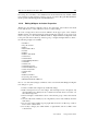
Changing the Default Text
It is possible to specify the default text that appears on an image by editing the file
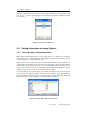
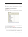
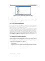
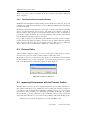
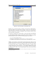
default_image_view.xml.
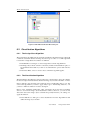
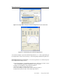
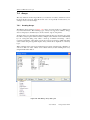
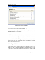
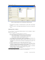
It is necessary to put this file in the appropriate folder for the portal you are using; these
folders are located in C:\Program Files\Definiens Developer XD 2.0.4\bin\application
(assuming you installed the program in the default location). By default, there are copies
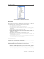
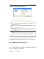
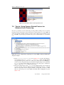
of default_image_view.xml in the Life and Tissue folders (figure 2.20) – if you wish to
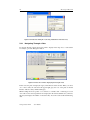
use this file for another portal, simply copy it into the appropriate folder.
Figure 2.20. Location of default_image_view.xml file
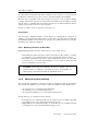
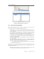
Open the xml file using Notepad (or your preferred editor) and look for the following
code:
<TopLeft></TopLeft>
<TopRight></TopRight>
<BottomLeft></BottomLeft>
<BottomRight></BottomRight>
Enter the text you want to appear by placing it between the relevant containers, for example:
<TopLeft>Sample_Text</TopLeft>
You will need to restart Definiens Developer XD 2.0.4 to view your changes.
27 September 2012
User Guide
Starting Developer
23
Inserting a Field
In the same way as described in the previous section, you can also insert the feature codes
that are used in the Edit Text Settings box into the xml.
For example, changing the xml container to <TopLeft> {#Active pixel x-value
Active pixel x,Name}: {#Active pixel x-value Active pixel x, Value}
</TopLeft> will display the name and x-value of the selected pixel.
Inserting the code APP_DEFAULT into a container will display the default values (map
number and slice number).
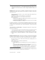
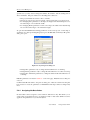
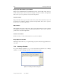
2.5.8
Navigating in 2D
The following mouse functions are available when navigating 2D images:
• The left mouse button is used for normal functions such as moving and selecting
objects
• Holding down the right mouse button and moving the pointer from left to right
adjusts window leveling on page 18
• To zoom in and out, either:
– Use the mouse wheel
– Hold down the Ctrl key and the right mouse button, then move the mouse up
and down.
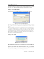
2.5.9
3D and 4D Viewing
The map features of Definiens Developer XD 2.0.4 also let you investigate:
• Three-dimensional images, made up of slices of 2D images
• Four-dimensional images, where a sequence of 3D frames changes over time
• Time series data sets, which corresponds to a continuous film image.
There are several options for viewing and analyzing image data represented by Definiens
maps. You can view three-dimensional, four-dimensional, and time series data using
specialized visualization tools. Using the map view, you can also explore three or fourdimensional data in several perspectives at once, and also compare the features of two
maps.
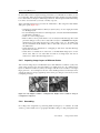
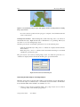
Viewing Image Data in 3D and Over Time
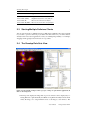
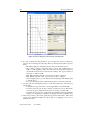
The 3D image objects display and the planar projections allow you to view objects in 3D
while simultaneously investigating them in 2D slices.
You can select from among six different split-screen views (figure 2.21) of the image data
and use the 3D Settings toolbar to navigate through slices, synchronize settings in one
projection with others, and change the data range. To display the 3D toolbar, go to View
> Toolbars > 3D.
User Guide
27 September 2012
24
Developer XD 2.0.4
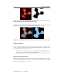
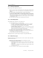
Figure 2.21. Map view with three planar projections and 3D image objects. (Image data
courtesy of Merck & Co., Inc.)
The 3D Toolbar
From left-to-right, you can use the toolbar buttons to perform the following functions:
•
•
•
•
•
•
•
•
•
•
•
Class Filter: Select classes to display as 3D objects
3D Visualization Options: Adjust the surface detail of 3D image objects
Window Layout: Select a layout for planar projections and 3D image objects
Navigation: Use sliders to navigate in the planar projections
Crosshairs: Display crosshairs in the planar projections
Start/Stop Animation: Start and stop animation of a time series
Show Next Slice: Display next slice in the planar projections
Show Previous Slice: Display previous slice in the planar projections
Show Next Time Frame: Display next time frame in the planar projections
Show Previous Time Frame: Display next time frame in the planar projections
Synchronize Views: Synchronize view settings across planar projections.
TIP: If 3D rendering is taking too long, you can stop it by unchecking the
classes in the Class Filter dialog.
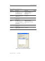
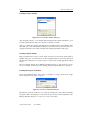
The Window Layout button in the 3D Toolbar allows you
to choose from the available viewing options. Standard XYZ co-ordinates are used (figure 2.22).
Selecting a Window Layout
From left to right, the following views are available:
27 September 2012
User Guide
Starting Developer
25
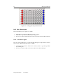
Figure 2.22. Standard XYZ co-ordinates for 3D objects
•
•
•
•
•
•
•
•
•
•
•
•
XY Planar Projection
XZ Planar Projection
YZ Planar Projection
3D Image Object
MPR Comparison View. (The Multi-Planar Preprojection (MPR) Comparison
View is two vertically arranged displays of the same projection. It is designed to
enable you to view two different maps, or to display different view settings. If you
are viewing only one map you can also access the split viewing modes available in
the Window menu.)
XY & XZ (displays a vertical side-by-side view)
XY & YZ (displays a vertical side-by-side view)
MPR Comparison View (as previously summarized but displayed horizontally.)
XY & XZ (displays horizontal side-by-side view.)
XY & YZ (displays horizontal side-by-side view.)
MPR (displays the multi-planar reprojection, including 3D image objects.)
Comparison View. (Displays two vertical groups with one of each planar projections in each group. This display enables you to view a different map in each group.
The two groups synchronize independently of each other.)
Select one or more classes of image objects to display
in the 3D image objects display. This display renders the surface of the selected image
objects in their respective class colors.
Displaying Image Objects in 3D
1. To display image objects in 3D, click the Window layout button in the 3D Settings
toolbar and select the 3D Image Objects button or the Multi-Planar Reprojection
button to open the 3D image objects display
User Guide
27 September 2012
26
Developer XD 2.0.4
2. Click the Class filter button to open the Edit Classification Filter dialog box and
check the boxes beside the classes you want to display. Click OK to display your
choices.
Several options are available to manipulate the image objects in the
3D image objects display. The descriptions use the analogy of a camera to represent the
user’s point of view:
Navigating in 3D
• Hold down the left mouse button to freely rotate the image in three dimensions by
dragging the mouse
• Ctrl + left mouse button rotates the image in x and y dimensions
• Shift + left mouse button moves the image around the window
• To zoom in and out:
– Holding down the right mouse button and moving the mouse up and down
zooms in and out with a high zoom factor
– Holding down the right mouse button and moving the mouse left and right
zooms in and out with a low zoom factor.
To enhance performance, you can click the 3D Visualization Options button in the 3D
Settings toolbar and use the slider to lower the detail of the 3D image objects. When
you select a 3D connected image object it will automatically be selected in the planar
projections.
Setting Transparency for 3D Image Objects
Changing the transparency of image objects
allows better visualization:
1. Open the Classification menu from the main menu bar and select Class Legend. If
you are using Developer XD you can also access the Class Hierarchy window
2. Right-click on a class and click Transparency (3D Image Objects) to open the slider
3. Move the slider to change the transparency. A value of 0 indicates an opaque
object. 1
There are several ways to navigate slices in the planar
projections. The slice number and orientation are displayed in the bottom right-hand
corner of the map view. If there is more than one map, the map name is also displayed.
Navigating the Planar Projections
• Reposition the cursor and crosshairs in three dimensions by clicking inside one of
the planar projections.
• Turn crosshairs off or on with the Crosshairs button.
• To move through slices:
– Select a planar projection and click the green arrows in the 3D Settings toolbar
– Use the mouse wheel (holding down the mouse wheel and moving the mouse
up and down will move through the slices more quickly)
– Click the Navigation button in the 3D Settings toolbar to open Slice Position
sliders that display the current slice and the total slices in each dimension.
1. Any image object with transparency setting greater than zero is ignored when selected; the image object is not
simultaneously selected in the planar projections. At very low transparency settings, some image objects may
flip 180 degrees. Raise the transparency to a higher setting to resolve this issue.
27 September 2012
User Guide
Starting Developer
27
– Use PgUp or PgDn buttons on the keyboard.
• You can move an object in the window using the keyboard arrow keys. If you hold
down the Ctrl key at the same time, you can move down the vertical scroll bar
• To zoom in and out, hold down the Ctrl key and the right mouse button, and move
the mouse up or down
• Holding down the right mouse button and moving the pointer from left to right
adjusts window leveling on page 18
Change the view settings, image object levels and image layers in one planar projection and then apply those settings to the other projections.
For the MPR Comparison view, synchronization is only possible for XY projections with
the same map.
Synchronizing Planar Projections
You can also use this tool to synchronize the map view after splitting using the options
available in the Window menu. Select one of the planar projections and change any of
the functions below. Then click the Sync button in the 3D settings toolbar to synchronize
the changes among all open projections.
•
•
•
•
•
Show or Hide Outlines
Pixel View or Object Mean View
View Classification
View Layer
Zoom options include Area Zoom, Zoom In Center, Zoom Out Center, Zoom In,
Zoom Out, Select Zoom Value, Zoom 100% and Zoom to Window. After zooming in one projection and then synchronizing, you can refocus all projections by
clicking on any point of interest.
• Image layers and image object level mixing.
• Image object levels
• Show/Hide Polygons and Show/Hide Skeletons (for 2D connected image objects
only).
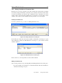
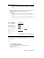
Customizing the Window Layout
To customize your window layouts and save them along
with the selected view settings:
1. Create a customized window layout by opening a window layout and choosing the
view settings you want to keep for each projection
2. Select View > Save Current Splitter Layout in the main menu to open the Save
Custom Layout dialog box
3. Choose a layout label (Custom 1 through Custom 7) and choose synchronization
options for planar projections. The options are:
• None: The Sync button is inoperative; it will not synchronize view settings,
crosshairs, or zoom settings in any of the projections
• By rows: The Sync button operates only across rows of the display
• By columns: The Sync button operates only across columns of the display
• All: The Sync button synchronizes all planar projections displayed
4. Click OK to save the layout. It is saved to the user information on the computer.
Viewing a Time Series Image data that includes a time series can be viewed as an animation. You can also step though frames one at a time. The current frame number displays
in the bottom right corner of the map view.
User Guide
27 September 2012
28
Developer XD 2.0.4
To view an animation of an open project, click the play button in the Animation toolbar;
to stop, click again. You can use the slider in the Animation toolbar to move back and
forth through frames. Either drag the slider or click it and then use the arrow keys on
your keyboard to step through the frames. You can also use buttons in the 3D Settings
toolbar to step back and forth through frames.
27 September 2012
User Guide
3
3.1
An Introductory Tutorial
Identifying Shapes
As an introduction to Definiens image analysis, we’ll analyze a very simple image. The
example is very rudimentary, but will give you an overview of the working environment.
The key concepts are the segmentation and classification of image objects; in addition, it
will familiarize you with the mechanics of putting together a rule set.
Figure 3.1. Screenshot displaying shapes.tif
Download the image shapes.tif and open it by going to File>New Project. When you
press Save or Save As, Developer XD uses this image to create a project (an additional
file will be created with the extension .dpr) and the Create Project dialog will appear.
Name the new project ‘Shape Recognition’, keep the default settings and press OK.
Of course, shapes.tif is a raster image and to start any meaningful analysis, we have to
instruct the software to recognize the elements as objects; after we’ve done this, we can
then add further levels of classification. In Definiens software, these instructions are
called rule sets and they are written and displayed in the Process Tree window.
29
30
3.1.1
Developer XD 2.0.4
Divide the Image Into Basic Objects
The first step in any analysis is for the software to divide up the image into defined areas –
this is called segmentation and creates undefined objects. By definition, these objects will
be relatively crude, but we can refine them later on with further rule sets. It is preferable
to create fairly large objects, as smaller numbers are easier to work with.
Right-click in the Process Tree window and select Append New from the right-click
menu. The Edit Process dialog appears. In the Name field, enter ‘Create objects and
remove background’. Press OK.
TIP: In the Edit Process box, you have the choice to run a process immediately (by pressing Execute) or to save it to the Process Tree window for
later execution (by pressing OK).
In the Process Tree window, right-click on this new rule and select Insert Child. In the
Algorithm drop-down box, select Multiresolution Segmentation. In the Segmentation Settings, which now appear in the right-hand side of the dialog box, change Scale Parameter
to 50. Press Execute.
The image now breaks up into large regions. When you now click on parts of the image,
you’ll see that – because our initial images are very distinct – the software has isolated
the shapes fairly accurately. It has also created several large objects out of the white
background.
NOTE: This action illustrates the parent-child concept in Definiens Developer XD 2.0.4. It’s possible to keep using Append New to add more and
more rules, but it’s best to group related rules in a container (a parent process), when you want a series of processes to create a particular outcome.
You can achieve this by adding sibling processes to the parent process, using the Insert Child command.
For more information on segmentation, see Multiresolution Segmentation (p 44); for
more detailed information, consult the Reference Book.
3.1.2
Identifying the Background
Overview
The obvious attribute of the background is that it is very homogeneous and, in terms of
color, distinct from the shapes within it.
In Developer XD you can choose from a huge number of shape, texture and color variables in order to classify a particular object, or group of objects. In this case, we’re going
to use the Brightness feature, as the background is much brighter then the shapes.
You can take measurements of these attributes by using the Feature View window. The
Feature View window essentially allows you test algorithms and change their parameters;
double-click on a feature of interest, then point your mouse at an object to see what
27 September 2012
User Guide
An Introductory Tutorial
31
numerical value it gives you. This value is displayed in the Image Object Information
window. You can then use this information to create a rule.
TIP: Running algorithms and changing values from the Feature View tree
does not affect any image settings in the project file or any of the rule sets.
It is safe to experiment with different settings and algorithms.
Writing the Rule Set
From the Feature View tree, select Object Features > Layer Values > Mean, then doubleclick on the Brightness tag. A Brightness value now appears in the Image Object Information window. Clicking on our new object primitives now gives a value for brightness and
the values are all in the region of 254. Conversely, the shapes have much lower brightness
values (between 80 and 100). So, for example, what we can now do is define anything
with a brightness value of more than 250 as background.
Right-click on the sibling you just created (the ‘200 [shape: 0.1 . . . ’ process) and select
Append New – this will create a new rule at the same level. (Once we’ve isolated the
background we’re going to stick the pieces together and give it the value ‘Background’.)
In the Algorithm drop-down box, select Assign Class. We need to enter the brightness
attributes we’ve just identified by pressing the ellipsis (. . . ) in the value column next
to Threshold Condition, which launches the Select Single Feature window. This has
a similar structure to the Feature View box so, as previously, select Object Features >
Layer Values > Mean and double-click on Brightness. We can define the background as
anything with a brightness over 230, so select the ‘greater than’ button (>) and enter 230
in the left-hand field. Press OK.
The final thing to do is to classify our new criteria. In the Use Class parameter of Algorithm Parameters on the right of the Edit Process window, overwrite ‘unclassified’, enter
‘Background’ and press Enter. The Class Description box will appear, where you can
change the color to white. Press OK to close the box, then press Execute in the Edit
Process dialog.
TIP: It’s very easy at this stage to miss out a function when writing rule
sets. Check the structure and the content of your rules against the screen
capture of the Process Tree window at the end of this section.
As a result, when you point your mouse at a white region, the Background classification
we have just created appears under the cursor. In addition, ‘Background’ now appears in
the Class Hierarchy window at the top right of the screen. Non-background objects (all
the shapes) have the classification ‘Unclassified’.
Joining the Background Pieces
As we’ve now got several pieces of background with a ‘Background’ classification, we
can merge all the pieces together as a single object.
User Guide
27 September 2012
32
Developer XD 2.0.4
Again, right-click on the last rule set in the Process Tree and select Append New, to create
the third rule in the ‘Create objects and remove background’ parent process.
In the Algorithm drop-down box, select Merge Region. In the Class Filter parameter,
which launches the Edit Classification Filter box, select ‘Background’ – we want to merge
the background objects so we can later sub-divide the remaining objects (the shapes).
Press OK to close the box, then press Execute. The background is now a single object.
TIP: To view the classification of an image object within an image, you
must have the View Classification button selected on the horizontal toolbar.
The classification is displayed when you hover over the object with the
cursor.
3.1.3
Shapes and Their Attributes
Some properties of circles:
• Small circumference in relation to area
• Constant degree of curvature
• No straight edges
Some properties of squares:
• A ratio of length to width of 1:1
• All sides are of equal length
Some properties of stars:
• Relatively long borders compared to area
• No curved edges
Isolating the Circles
Developer XD has a built-in algorithm called Elliptic Fit; it basically measures how
closely an object fits into an ellipse of a similar area. Elliptic Fit can also be found in
Feature View and can be found by selecting Object Features > Geometry > Shape, then
double-clicking on Elliptic Fit. Of course a perfect circle has an elliptic fit of 1 (the maximum value), so – at least in this example – we don’t really need to check this. But you
might want to practice using Feature View anyway.
To isolate the circles, we need to set up a new rule. We want this rule to be in the same
hierarchical level as our first ‘Create objects . . . ’ rule set and the easiest way to do this is
to right-click on the ‘Create objects’ rule set and select Append New, which will create a
process at the same level. Call this process ‘Define and isolate circles’.
To add the rule, right-click the new process and select Insert Child. In the Algorithm
drop-down box, select Assign Class. Click on Threshold Condition to navigate towards
the Elliptic Fit algorithm, using the path describe earlier. To allow for a bit of image
27 September 2012
User Guide
An Introductory Tutorial
33
degradation, we’re going to define a circle as anything with a value of over 0.95 – click
on the ‘greater than’ symbol and enter the value 0.95. Press OK.
Back in the Edit Process window, we will give our classification a name. Replace the
‘unclassified’ value in Use Class with ‘Circle’, press enter and assign it a color of your
choosing. Press OK. Finally, in the Edit Process window, press Execute to run the process.
There is now a ‘Circle’ classification in the class hierarchy and placing your cursor over
the circle shape will display the new classification.
Isolating the Squares
There is also a convenient algorithm we can use to identify squares; the Rectangular Fit
value (which for a square is, of course, one).
The method is the same as the one for the circle – create a new parent class and call
it ‘Define and isolate squares’ When you create the child, you will be able to find the
algorithm by going to Object Features > Geometry > Shape > Rectangular. Set the range
to ‘=1’ and assign it to a new class (‘Square’).
Isolating the Star
There are criteria you could use to identify the star but as we’re using the software to
separate and classify squares, circles and stars, we can be pragmatic – after defining
background, circles and squares, the star is the only objects remaining. So the only thing
left to do is to classify anything ‘unclassified’ as a star.
Simply set up a parent called ‘Define and isolate stars’, select Assign Class, select ‘unclassified’ in the Class Filter and give it the value ‘Star’ in Use Class.
3.1.4
The Complete Rule Set
Figure 3.2. Complete rule set list for shapes tutorial
User Guide
27 September 2012
4
Basic Rule Set Editing
4.1
Creating and Editing Processes in the Process Tree
Window
Rule sets are built up from single processes, which are displayed in the Process Tree and
created using the Edit Process dialog box. A single process can operate on two levels; at
the level of image objects (created by segmentation), or at the pixel level. Whatever the
object, a process will run sequentially through each target, applying an algorithm to each.
This section builds upon the tutorial in the previous chapter.
Figure 4.1. The Process Tree window displaying a simple rule set
There are three ways to open the Edit Process dialog box (figure 4.2):
• Right-click on the Process Tree window and select Append New
• Select Process > Process Commands > Append New from the main menu
• Use the keyboard shortcut Ctrl+ A .
The main areas in the Edit Process dialog box are listed in the following sections.
4.1.1
Name
Naming of processes is automatic, unless the Automatic check-box is unchecked and a
name is added manually. Processes can be grouped together and arranged into hierarchies,
which has consequences around whether or not to use automatic naming – this is covered
in Parent and Child Processes on page 40.
4.1.2
Algorithm
The Algorithm drop-down box allows the user to select an algorithm or a related process. Depending on the algorithm selected, further options may appear in the Algorithm
Parameters pane.
35
36
Developer XD 2.0.4
Figure 4.2. The Edit Process dialog box
4.1.3
Image Object Domain
This defines the image objects (p 2) on which algorithms operate.
4.1.4
Algorithm Parameters
This defines the individual settings of the algorithm in the Algorithms Parameters group
box. (We recommend you do this after selecting the image object domain.)
4.2
4.2.1
Adding a Process
Selecting and Configuring an Image Object Domain
An algorithm can be applied to several objects of interest – in Definiens software, these
are called image object domains. This allows you to narrow down the objects of interest
and therefore the number of objects on which algorithms act.
For many algorithms, you can define the image object domain by selecting a level within
the image object hierarchy. Typical targets may be the pixel level, an image object level,
or specified image objects. (When using the pixel level, the process creates a new image
object level.)
Depending on the algorithm, you can choose among different basic domains and specify
your choice by setting execution parameters. Common parameters are:
27 September 2012
User Guide
Basic Rule Set Editing
37
• Level: If you choose image object level for the image object domain, you must
select an image object level name or a variable. If you choose pixel level for the
image object domain, you can specify the name of a new image object level.
• Class filter: If you already classified image objects, you can select classes to focus
on the image objects of these classes.
• Threshold condition: You can use a threshold condition to further narrow down the
number of image objects. When you have added a threshold condition, a second
drop-down box appears, which allows you to add another threshold condition.
• Max. number of image objects: Enter the maximum number of image objects to
be processed.
Technically, the image object domain is a set of image objects. Every process loops
through the set of image objects in the image object domain, one-by-one, and applies the
algorithm to each image object.
The set of domains is extensible, using the Developer XD SDK. To specify the image
object domain, select an image object level or another basic domain in the drop-down list.
Available domains are listed in table 4.1 on the current page, Image Object Domains.
Table 4.1. Image Object Domains
Basic Domain
Usage
Parameters
Execute
A general domain used to execute an
Threshold condition; Map
algorithm. It will activate any commands you
define in the Edit Process dialog box, but is
independent of any image objects. It is
commonly used to enable parent processes to
run their subordinate processes (Execute
Child Process) or to update a variable
(Update Variable): Combined with threshold
– if; Combined with map – on map;
Threshold + Loop While Change – while
Pixel level
Applies the algorithm to the pixel level.
Typically used for initial segmentations and
filters
Map; Threshold condition
Image object
level
Applies the algorithm to image objects on an
image object level. Typically used for object
processing
Level; Class filter;
Threshold condition; Map;
Region; Max. number of
image objects
Current image
object
Applies the algorithm to the current internally Class filter; Threshold
selected image object of the parent process.
condition; Max. number of
image objects
Neighbor image
object
Applies the algorithm to all neighbors of the Class filter; Threshold
current internally selected image object of the condition; Max. number of
parent process. The size of the neighborhood image objects; Distance
is defined by the Distance parameter.
Continues. . .
User Guide
27 September 2012
38
Developer XD 2.0.4
Basic Domain
Usage
Parameters
Super object
Applies the algorithm to the superobject of
the current internally selected image object
of the parent process. The number of levels
up the image objects level hierarchy is
defined by the Level Distance parameter.
Class filter; Threshold
condition; Level distance;
Max. number of image
objects
Sub objects
Applies the algorithm to all sub-objects of the
current internally selected image object of
the parent process. The number of levels
down the image objects level hierarchy is
defined by the Level Distance parameter.
Class filter; Threshold
condition; Level distance;
Max. number of image
objects
Linked objects
Applies the algorithm to the linked object of
the current internally selected image object
of the parent process.
Link class filter; Link
direction; Max distance;
Use current image object;
Class filter; Threshold
condition; Max. number of
image objects
Maps
Applies the algorithm to all specified maps of Map name prefix;
a project. You can select this domain in
Threshold condition
parent processes with the Execute child
process algorithm to set the context for child
processes that use the Map parameter From
Parent.
Image object list
A selection of image objects created with the
Update Image Object List algorithm.
Image object list; Class
filter; Threshold condition;
Max. number of image
objects
This set of domains is extensible using the Developer SDK.
4.2.2
Adding an Algorithm
Algorithms are selected from the drop-down list under Algorithms; detailed descriptions
of algorithms are available in the Reference Book.
By default, the drop-down list contains all available algorithms. You can customize this
list by selecting ‘more’ from the drop-down list, which opens the Select Process Algorithms box (figure 4.3).
By default, the ‘Display all Algorithms always’ box is selected. To customize the display,
uncheck this box and press the left-facing arrow under ‘Move All’, which will clear the
list. You can then select individual algorithms to move them to the Available Algorithms
list, or double-click their headings to move whole groups.
27 September 2012
User Guide
Basic Rule Set Editing
39
Figure 4.3. The Select Process Algorithms Dialog Box
4.2.3
Loops & Cycles
Loops & Cycles allows you to specify how many times you would like a process (and its
child processes) to be repeated. The process runs cascading loops based on a number you
define; the feature can also run loops while a feature changes (for example growing).
4.2.4
Executing a Process
To execute a single process, select the process in the Process Tree and press F5. Alternatively, right-click on the process and select Execute. If you have child processes below
your process, these will also be executed.
You can also execute a process from the Edit Process dialog box by pressing Execute,
instead of OK (which adds the process to the Process Tree window without executing it).
4.2.5
Executing a Process on a Selected Object
To execute a process on an image object that as already been defined by a segmentation
process, select the object then select the process in the Process Tree. To execute the
process, right-click and select Execute on Selected Object or press F6.
User Guide
27 September 2012
40
4.2.6
Developer XD 2.0.4
Parent and Child Processes
The introductory tutorial (p 29) will have introduced you to the concept of parent and
child processes. Using this hierarchy allows you to organize your processes in a more
logical way, grouping processes together to carry out a specific task.
Go to the Process Tree and right-click in the window. From the context menu, choose
Append New. the Edit Process dialog (figure 4.2) will appear. This is the one time it is
recommended that you deselect automatic naming and give the process a logical name,
as you are essentially making a container for other processes. By default, the algorithm
drop-down box displays Execute Child Processes. Press OK.
You can then add subordinate processes by right-clicking on your newly created parent
and selecting Insert Child. We recommend you keep automatic naming for these processes, as the names display information about the process. Of course, you can select
child process and add further child processes that are subordinate to these.
Figure 4.4. Rule set sample showing parent and child processes
4.2.7
Editing a Rule Set
You can edit a process by double-clicking it or by right-clicking on it and selecting Edit;
both options will display the Edit Process dialog box.
What is important to note is that when testing and modifying processes, you will often
want to re-execute a single process that has already been executed. Before you can do
this, however, you must delete the image object levels that these processes have created.
In most cases, you have to delete all existing image object levels and execute the whole
process sequence from the beginning. To delete image object levels, use the Delete Levels
button on the main toolbar (or go to Image Objects > Delete Level(s) via the main menu).
It is also possible to delete a level as part of a rule set (and also to copy or rename one). In
the Algorithm field in the Edit Process box, select Delete Image Object Level and enter
your chosen parameters.
4.2.8
Undoing Edits
It is possible to go back to a previous state by using the undo function, which is located in
Process > Undo (a Redo command is also available). These functions are also available
27 September 2012
User Guide
Basic Rule Set Editing
41
as toolbar buttons using the Customize command. You can undo or redo the creation,
modification or deletion of processes, classes, customized features and variables.
However, it is not possible to undo the execution of processes or any operations relating
to image object levels, such as Copy Current Level or Delete Level. In addition, if items
such as classes or variables that are referenced in rule sets are deleted and then undone,
only the object itself is restored, not its references.
It is also possible to revert to a previous version (p 194).
Undo Options
You can assign a minimum number of undo actions by selecting Tools > Options; in
addition, you can assign how much memory is allocated to the undo function (although
the minimum number of undo actions has priority). To optimize memory you can also
disable the undo function completely.
4.2.9
Deleting a Process or Rule Set
Right-clicking in the Process Tree window gives you two delete options:
• Delete Rule Set deletes the entire contents of the Process Tree window – a dialog
box will ask you to confirm this action. Once performed, it cannot be undone
• The Delete command can be used to delete individual processes. If you delete
a parent process, you will be asked whether or not you wish to delete any subprocesses (child processes) as well
CAUTION: Delete Rule Set eliminates all classes, variables, and customized features, in addition to all single processes. Consequently, an
existing image object hierarchy with any classification is lost.
4.2.10
Editing Using Drag and Drop
You can edit the organization of the Process Tree by dragging and dropping with the
mouse. Bear in mind that a process can be connected to the Process Tree in three ways:
• As a parent process on a higher hierarchical level
• As a child process on a lower hierarchy level
• As an appended sibling process on the same hierarchy level.
To drag and drop, go to the Process Tree window:
• Left-click a process and drag and drop it onto another process. It will be appended
as a sibling process on the same level as the target process
• Right-click a process and drag and drop it onto another process. It will be inserted
as a child process on a lower level than the target process.
User Guide
27 September 2012
42
Developer XD 2.0.4
4.3
Creating Image Objects Through Segmentation
Commonly, the term segmentation means subdividing entities, such as objects, into
smaller partitions. In Developer XD it is used differently; segmentation is any operation that creates new image objects or alters the morphology of existing image objects
according to specific criteria. This means a segmentation can be a subdividing operation,
a merging operation, or a reshaping operation.
There are two basic segmentation principles:
• Cutting something big into smaller pieces, which is a top-down strategy
• Merging small pieces to get something bigger, which is a bottom-up strategy.
An analysis of which segmentation method to use with which type of image is beyond
the scope of this guide; all the built-in segmentation algorithms have their pros and cons
and a rule-set developer must judge which methods are most appropriate for a particular
image analysis.
4.3.1
Top-down Segmentation
Top-down segmentation means cutting objects into smaller objects. It can – but does not
have to – originate from the entire image as one object. Definiens Developer XD 2.0.4
offers three top-down segmentation methods: chessboard segmentation, quadtree-based
segmentation and multi-threshold segmentation.
Multi-threshold segmentation is the most widely used; chessboard and quadtree-based
segmentation are generally useful for tiling and dividing objects into equal regions.
Chessboard Segmentation
Chessboard segmentation is the simplest segmentation algorithm. It cuts the scene or –
in more complicated rule sets – the dedicated image objects into equal squares of a given
size.
Figure 4.5. Chessboard segmentation
Because the Chessboard Segmentation algorithm produces simple square objects, it is
often used to subdivide images and image objects. The following are some typical uses:
• Refining small image objects: Relatively small image objects, which have already
been identified, can be segmented with a small square-size parameter for more
detailed analysis. However, we recommend that pixel-based object resizing should
be used for this task.
27 September 2012
User Guide
Basic Rule Set Editing
43
• Applying a new segmentation: Let us say you have an image object that you want
to cut into multiresolution-like image object primitives. You can first apply chessboard segmentation with a small square size, such as one, then use those square
image objects as starting image objects for a multiresolution segmentation.
You can use the Edit Process dialog box to define the size of squares.
• Object Size: Use an object size of one to generate pixel-sized image objects. The
effect is that for each pixel you can investigate all information available from features
• Medium Square Size: In cases where the image scale (resolution or magnification)
is higher than necessary to find regions or objects of interest, you can use a square
size of two or four to reduce the scale. Use a square size of about one-twentieth to
one-fiftieth of the scene width for a rough detection of large objects or regions of
interest. You can perform such a detection at the beginning of an image analysis
procedure.
Quadtree-Based Segmentation
Quadtree-based segmentation is similar to chessboard segmentation, but creates squares
of differing sizes. You can define an upper limit of color differences within each square
using Scale Parameter. After cutting an initial square grid, the quadtree-based segmentation continues as follows:
• Cut each square into four smaller squares if the homogeneity criterion is not met.
Example: The maximal color difference within the square object is larger than the
defined scale value.
• Repeat until the homogeneity criterion is met at each square.
Figure 4.6. Quadtree-based segmentation
Following a quadtree-based segmentation, very homogeneous regions typically produce
larger squares than heterogeneous regions. Compared to multiresolution segmentation,
quadtree-based segmentation is less heavy on resources.
Contrast Filter Segmentation
Contrast filter segmentation is a very fast algorithm for initial segmentation and, in some
cases, can isolate objects of interest in a single step. Because there is no need to initially
create image object primitives smaller than the objects of interest, the number of image
objects is lower than with some other approaches.
User Guide
27 September 2012
44
Developer XD 2.0.4
An integrated reshaping operation modifies the shape of image objects to help form coherent and compact image objects. The resulting pixel classification is stored in an internal
thematic layer. Each pixel is classified as one of the following classes: no object, object in first layer, object in second layer, object in both layers and ignored by threshold.
Finally, a chessboard segmentation is used to convert this thematic layer into an image
object level.
In some cases you can use this algorithm as first step of your analysis to improve overall
image analysis performance substantially. The algorithm is particularly suited to fluorescent images where image layer information is well separated.
Contrast Split Segmentation
Contrast split segmentation is similar to the multi-threshold segmentation approach. The
contrast split segments the scene into dark and bright image objects based on a threshold
value that maximizes the contrast between them.
The algorithm evaluates the optimal threshold separately for each image object in the
image object domain. Initially, it executes a chessboard segmentation of variable scale
and then performs the split on each square, in case the pixel level is selected in the image
object domain.
Several basic parameters can be selected, the primary ones being the layer of interest and
the classes you want to assign to dark and bright objects. Optimal thresholds for splitting
and the contrast can be stored in scene variables.
4.3.2
Bottom-up Segmentation
Bottom-up segmentation means assembling objects to create a larger objects. It can –
but does not have to – start with the pixels of the image. Examples are multiresolution
segmentation and classification-based segmentation.
Multiresolution Segmentation
The Multiresolution Segmentation algorithm 1 consecutively merges pixels or existing
image objects. Essentially, the procedure identifies single image objects of one pixel in
size and merges them with their neighbors, based on relative homogeneity criteria. This
homogeneity criterion is a combination of spectral and shape criteria.
You can modify this calculation by modifying the scale parameter. Higher values for the
scale parameter result in larger image objects, smaller values in smaller ones.
With any given average size of image objects, multiresolution segmentation yields good
abstraction and shaping in any application area. However, it puts higher demands on the
processor and memory, and is significantly slower than some other segmentation techniques – therefore it may not always be the best choice.
1. Benz UC, Hofmann P, Willhauck G, Lingenfelder M (2004). Multi-Resolution, Object-Oriented Fuzzy Analysis
of Remote Sensing Data for GIS-Ready Information. SPRS Journal of Photogrammetry & Remote Sensing, Vol
58, pp239–258. Amsterdam: Elsevier Science
27 September 2012
User Guide
Basic Rule Set Editing
45
The homogeneity criterion of the multiresolution segmentation algorithm measures how homogeneous or heterogeneous an image object is within
itself. It is calculated as a combination of the color and shape properties of the initial and
resulting image objects of the intended merging.
The Homogeneity Criterion
Color homogeneity is based on the standard deviation of the spectral colors. The shape
homogeneity is based on the deviation of a compact (or smooth) shape. 2 Homogeneity
criteria can be customized by weighting shape and compactness criteria:
• The shape criterion can be given a value of up to 0.9. This ratio determines to what
degree shape influences the segmentation compared to color. For example, a shape
weighting of 0.6 results in a color weighting of 0.4
• In the same way, the value you assign for compactness gives it a relative weighting
against smoothness.
Multi-Threshold Segmentation and Auto Thresholds
The Multi-Threshold Segmentation algorithm is a new feature in Definiens Developer
XD 2.0.4. It splits the image object domain and classifies the resulting image objects
based on a defined pixel value threshold. This threshold can be user-defined or can be
auto-adaptive when used in combination with the Automatic Threshold algorithm.
The threshold can be determined for an entire scene or for individual image objects; this
determines whether it is stored in a scene variable or an object variable, dividing the selected set of pixels into two subsets so that heterogeneity is increased to a maximum. The
algorithm uses a combination of histogram-based methods and the homogeneity measurement of multi-resolution segmentation to calculate a threshold dividing the selected set
of pixels into two subsets.
Spectral Difference Segmentation
Spectral difference segmentation lets you merge neighboring image objects if the difference between their layer mean intensities is below the value given by the maximum
spectral difference. It is designed to refine existing segmentation results, by merging
spectrally similar image objects produced by previous segmentations and therefore is a
bottom-up segmentation.
The algorithm cannot be used to create new image object levels based on the pixel level.
4.3.3
Segmentation by Reshaping Algorithms
All algorithms listed under the Reshaping Algorithms 3 group technically belong to the
segmentation strategies. Reshaping algorithms cannot be used to identify undefined image objects, because these algorithms require pre-existing image objects. However, they
are useful for getting closer to regions and image objects of interest.
2. The Multiresolution Segmentation algorithm criteria Smoothness and Compactness are not related to the features of the same name.
3. Sometimes reshaping algorithms are referred to as classification-based segmentation algorithms, because they
commonly use information about the class of the image objects to be merged or cut. Although this is not always
true, Definiens Developer XD 2.0.4 uses this terminology.
User Guide
27 September 2012
46
Developer XD 2.0.4
NOTE: Sometimes reshaping algorithms are referred to as classificationbased segmentation algorithms, because they commonly use information
about the class of the image objects to be merged or cut. Although this is
not always true, Definiens Developer XD 2.0.4 uses this terminology.
The two most basic algorithms in this group are Merge Region and Grow Region. The
more complex Image Object Fusion is a generalization of these two algorithms and offers
additional options.
Merge Region
The Merge Region algorithm merges all neighboring image objects of a class into one
large object. The class to be merged is specified in the image object domain. 4
Figure 4.7. Red image objects are merged
Classifications are not changed; only the number of image objects is reduced.
Grow Region
The Grow Region 5 algorithm extends all image objects that are specified in the image
object domain, and thus represent the seed image objects. They are extended by neighboring image objects of defined candidate classes. For each process execution, only those
candidate image objects that neighbor the seed image object before the process execution
are merged into the seed objects. The following sequence illustrates four Grow Region
processes:
4. The image object domain of a process using the Merge Region algorithm should define one class only. Otherwise, all objects will be merged irrespective of the class and the classification will be less predictable.
5. Grow region processes should begin the initial growth cycle with isolated seed image objects defined in the
image object domain. Otherwise, if any candidate image objects border more than one seed image objects,
ambiguity will result as to which seed image object each candidate image object will merge with.
27 September 2012
User Guide
Basic Rule Set Editing
47
Figure 4.8. Red seed image objects grow stepwise into green candidate image objects
4.4
Object Levels and Segmentation
Although you can perform some image analysis on a single image object level, the full
power of the Definiens object-oriented image analysis unfolds when using multiple levels.
On each of these levels, objects are defined by the objects on the level below them that
are considered their sub-objects. In the same manner, the lowest level image objects are
defined by the pixels of the image that belong to them. This concept has already been
introduced in Image Object Hierarchy.
4.4.1
About Hierarchical Image Object Levels
The levels of an image object hierarchy range from a fine resolution of image objects on
the lowest level to the coarse resolution on the highest. On its superlevel, every image
object has only one image object, the superobject. On the other hand, an image object
may have – but is not required to have – multiple sub-objects.
To better understand the concept of the image object hierarchy, imagine a hierarchy of
image object levels, each representing a meaningful structure in an image. These levels
are related to the various (coarse, medium, fine) resolutions of the image objects. The
hierarchy arranges subordinate image structures (such as a cell) below generic image
structures (such as tissue); figure 4.9 on the following page shows some biological and
geographical examples.
The lowest and highest members of the hierarchy are unchanging; at the bottom is the
digital image itself, made up of pixels, while at the top is a level containing a single
object (such as an organ or a forest).
4.4.2
Creating an Image Object Level
There are two ways to create an image object level:
• Applying a segmentation algorithm using the pixel-level domain will create a new
level. Image object levels are usually added above an existing ones, although some
algorithms let you specify whether new layers are created above or below existing
ones
• Using the Copy Image Object Level algorithm
User Guide
27 September 2012
48
Developer XD 2.0.4
Figure 4.9. Meaningful image object levels within an image object hierarchy
The shapes of image objects on these super- and sublevels will constrain the shape of the
objects in the new level.
The hierarchical network of an image object hierarchy is topologically definite. In other
words, the border of a superobject is consistent with the borders of its sub-objects. The
area represented by a specific image object is defined by the sum of its sub-objects’ areas;
Definiens technology accomplishes this quite easily, because the segmentation techniques
use region-merging algorithms. For this reason, not all the algorithms used to analyze
images allow a level to be created below an existing one.
Each image object level is constructed on the basis of its direct sub-objects. For example,
the sub-objects of one level are merged into larger image objects on level above it. This
merge is limited by the borders of exiting superobjects; adjacent image objects cannot be
merged if they have different superobjects.
4.4.3
Creating Object Levels With Segmentation Algorithms
You can create an image object level by using some segmentation algorithms such as
multiresolution segmentation, multi-threshold or spectral difference segmentation. The
relevant settings are in the Edit Process dialog box:
• Go to the drop-down list box within the Image Object Domain group box and select
an available image object level. To switch to another image object level, select the
27 September 2012
User Guide
Basic Rule Set Editing
49
currently active image object level and click the Parameters button to select another
image object level in the Select Level dialog box.
• Insert the new image object level either above or below the one selected in the
image object level. Go to the Algorithm Parameters group box and look for a Level
Usage parameter. If available, you can select from the options; if not available the
new image object level is created above the current one.
Using Segmentation to Create an Image Object Hierarchy
Because a new level produced by segmentation uses the image objects of the level beneath
it, the function has the following restrictions:
• An image object level cannot contain image objects larger than its superobjects or
smaller than its sub-objects
• When creating the first image object level, the lower limit of the image objects size
is represented by the pixels, the upper limit by the size of the scene.
This structure enables you to create an image object hierarchy by segmenting the image
multiple times, resulting in different image object levels with image objects of different
scales.
4.4.4
Duplicating an Image Object Level
It is often useful to duplicate an image object level in order to modify the copy. To
duplicate a level, do one of the following:
• Choose Image Objects > Copy Current Level from the main menu. The new image
object level will be inserted above the currently active one
• Create a process using the Copy Image Object Level algorithm. You can choose to
insert the new image object level either above or below an existing one.
4.4.5
Editing an Image Object Level or Level Variable
Figure 4.10. The Edit Level Aliases dialog box
User Guide
27 September 2012
50
Developer XD 2.0.4
You may want to rename an image object level name, for example to prepare a rule set for
further processing steps or to follow your organization’s naming conventions. You can
also create or edit level variables and assign them to existing levels.
1. To edit an image object level or level variable, select Image Objects > Edit Level
Names from the main menu. The Edit Level Aliases dialog box opens (figure 4.10)
2. Select an image object level or variable and edit its alias
3. To create a new image object level name, 6 type a name in the Alias field and click
the Add Level or Add Variable button to add a new unassigned item to the Level
Names or Variable column. Select ‘not assigned’ and edit its alias or assign another
level from the drop-down list. Click OK to make the new level or variable available
for assignment to a newly created image object level during process execution.
4. To assign an image object level or level variable to an existing value, select the item
you want to assign and use the drop-down arrow to select a new value.
5. To remove a level variable alias, select it in the Variables area and click Remove.
6. To rename an image object level or level variable, select it in the Variables area,
type a new alias in the Alias field, and click Rename.
Using Predefined Names
In some cases it is helpful to define names of image object levels before they are assigned
to newly created image object levels during process execution. To do so, use the Add
Level button within the Edit Level Aliases dialog box.
• Depending on the selected algorithm and the selected image object domain, you
can alternatively use one of the following parameters:
• Level parameter of the image object domain group box
• Level Name parameter in the Algorithm Parameters group box
Instead of selecting any item in the drop-down list, just type the name of the image object
level to be created during process execution. Click OK and the name is listed in the Edit
Level Aliases dialog box.
4.4.6
Deleting an Image Object Level
When working with image object levels that are temporary, or are required for testing
processes, you will want to delete image object levels that are no longer used. To delete
an image object level do one of the following:
• Create a process using the Delete Image Object Level algorithm
• Choose Image Objects > Delete Levels from the main menu or use the button on
the toolbar
The Delete Level dialog box (figure 4.11) will open, which displays a list of all image
object levels according to the image object hierarchy.
Select the image object level to be deleted (you can press Ctrl to select multiple levels)
and press OK. The selected image object levels will be removed from the image object
6. You can change the default name for new image object levels in Tools > Options
27 September 2012
User Guide
Basic Rule Set Editing
51
hierarchy. Advanced users may want to switch off the confirmation message before deletion. To do so, go to the Option dialog box and change the Ask Before Deleting Current
Level setting.
Figure 4.11. Delete Level dialog box
4.5
4.5.1
Getting Information on Image Objects
The Image Object Information Window
When analyzing individual images or developing rule sets you will need to investigate
single image objects. The Features tab of the Image Object Information window is used
to get information on a selected image object.
Image objects consist of spectral, shape, and hierarchical elements. These elements are
called features in Definiens Developer XD 2.0.4. The Feature tab in the Image Object
Information window displays the values of selected attributes when an image object is
selected from within the map view. The Image Object Information window is open by
default, but can also be selected from the View menu if required.
To get information on a specific image object click on an image object in the map view
(some features are listed by default). To add or remove features, right-click the Image
Object Information window and choose Select Features to Display. The Select Displayed
Features dialog box opens, allowing you to select a feature of interest.
Figure 4.12. Image Object Information window
User Guide
27 September 2012
52
Developer XD 2.0.4
The selected feature values are now displayed in the map view. To compare single image
objects, click another image object in the map view and the displayed feature values are
updated.
Figure 4.13. Map view of selected image object values. (Image data courtesy of EMBL Hei-
delberg)
Double-click a feature to display it in the map view; to deselect a selected image object,
click it in the map view a second time. If the processing for image object information
takes too long, or if you want to cancel the processing for any reason, you can use the
Cancel button in the status bar.
4.5.2
The Feature View Window
Image objects have spectral, shape, and hierarchical characteristics and these features are
used as sources of information to define the inclusion-or-exclusion parameters used to
classify image objects. There are two major types of features:
• Object features, which are attributes of image objects (for example the area of an
image object)
• Global features, which are not connected to an individual image object (for example the number of image objects of a certain class)
Available features are sorted in the feature tree, which is displayed in the Feature View
window (figure 4.14). It is open by default but can be also selected via Tools > Feature
View or View > Feature View.
This section lists a very brief overview of functions. For more detailed information, consult the Reference Book
27 September 2012
User Guide
Basic Rule Set Editing
53
Figure 4.14. Feature tree in the Feature View window
Object Features
Object features are calculated by evaluating image objects themselves as well as their
embedding in the image object hierarchy. They are grouped as follows:
• Customized features are user created
• Type features refer to an image object’s position in space
• Layer value features utilize information derived from the spectral properties of
image objects
• Geometry features evaluate an image object’s shape
• Position features refer to the position of an image object relative to a scene.
• Texture features allow texture values based on layers and shape. Texture after
Haralick is also available.
• Object Variables are local variables for individual image objects
• Hierarchy features provide information about the embedding of an image object
within the image object hierarchy.
• Thematic attribute features are used to describe an image object using information
provided by thematic layers, if these are present.
Class-Related Features
Class-related features are dependent on image object features and refer to the classes
assigned to image objects in the image object hierarchy.
This location is specified for superobjects and sub-objects by the levels separating them.
For neighbor image objects, the location is specified by the spatial distance. Both these
distances can be edited. Class-related features are grouped as follows:
• Relations to Neighbor Objects features are used to describe an image object by its
relationships to other image objects of a given class on the same image object level
• Relations to Sub-Objects features describe an image object by its relationships to
other image objects of a given class, on a lower image object level in the image
User Guide
27 September 2012
54
Developer XD 2.0.4
object hierarchy. You can use these features to evaluate sub-scale information because the resolution of image objects increases as you move down the image object
hierarchy
• Relations to Superobjects features describe an image object by its relations to other
image objects of a given class, on a higher image object level in the image object hierarchy. You can use these features to evaluate super-scale information because the
resolution of image objects decreases as you move up the image object hierarchy
• Relations to Classification features are used to find out about the current or potential classification of an image object.
Linked Object Features
Linked Object features are calculated by evaluating linked objects themselves.
Scene Features
Scene features return properties referring to the entire scene or map. They are global
because they are not related to individual image objects, and are grouped as follows:
• Variables are global variables that exist only once within a project. They are independent of the current image object.
• Class-Related scene features provide information on all image objects of a given
class per map.
• Scene-Related features provide information on the scene.
Process-Related Features
Process-related features are image object dependent features. They involve the relationship of a child process image object to a parent process. They are used in local processing.
A process-related features refers to a relation of an image objects to a parent process object (PPO) of a given process distance in the process hierarchy. Commonly used processrelated features include:
• Border to PPO: The absolute border of an image object shared with its parent process object.
• Distance to PPO: The distance between two parent process objects.
• Elliptic dist. from PPO is the elliptic distance of an image object to its parent
process object (PPO).
• Same super object as PPO checks whether an image object and its parent process
object (PPO) are parts of the same superobject.
• Rel. border to PPO is the ratio of the border length of an image object shared with
the parent process object (PPO) to its total border length.
Region Features
Region features return properties referring to a given region. They are global because
they are not related to individual image objects. They are grouped as follows:
27 September 2012
User Guide
Basic Rule Set Editing
55
• Region-related features provide information on a given region.
• Layer-related region features evaluate the first and second statistical moment
(mean, standard deviation) of a region’s pixel value.
• Class-related region features provide information on all image objects of a given
class per region.
Metadata
Metadata items can be used as a feature in rule set development. To do so, you have
to provide external metadata in the feature tree. If you are not using data import procedures to convert external source metadata to internal metadata definitions, you can create
individual features from a single metadata item.
Feature Variables
Feature variables have features as their values. Once a feature is assigned to a feature
variable, the variable can be used in the same way, returning the same value and the
assigned value. It is possible to create a feature variable without a feature assigned, but
the calculation value would be invalid.
Creating a New Feature
Most features with parameters must first be created before they are used and require
values to be set beforehand. Before a feature of image object can be displayed in the map
view, an image must be loaded and a segmentation must be applied to the map.
1. To create a new feature, right-click in the Feature View window and select Manage Customized Features. In the dialog box, click Add to display the Customized
Features box, then click on the Relational tab
2. In this example, we will create a new feature based on Min. Pixel Value. In the
Feature Selection box, this can be found by selecting Object Values > Layer Values
> Pixel-based > Min. Pixel Value
3. Under Min. Pixel Value, right-click on Create New ‘Min. Pixel Value’ and select
Create.
The relevant dialog box – in this case Min. Pixel Value (figure 4.15) – will open.
In this example, the parameter value will be set to Nuclei.
4. Depending on the feature and your project, you must set parameter values. Pressing
OK will list the new feature in the feature tree. The new feature will also be loaded
into the Image Object Information window
5. Some features require you to input a unit, which is displayed in parentheses in the
feature tree. By default the feature unit is set to pixels, but other units are available.
You can change the default feature unit for newly created features. Go to the Options
dialog box and change the default feature unit item from pixels to ‘same as project unit’.
The project unit is defined when creating the project and can be checked and modified in
the Modify Project dialog box.
User Guide
27 September 2012
56
Developer XD 2.0.4
Figure 4.15. [Feature] dialog box for creating a new feature from the Select Displayed Fea-
tures dialog box
Thematic Attributes
Thematic attributes can only be used if a thematic layer has been imported into the project.
If this is the case, all thematic attributes in numeric form that are contained in the attribute
table of the thematic layer can be used as features in the same manner as you would use
any other feature.
Object Oriented Texture Analysis
Object-oriented texture analysis allows you to describe image objects by their texture. By
looking at the structure of a given image object’s sub-objects, an object’s form and texture
can be determined. An important aspect of this method is that the respective segmentation
parameters of the sub-object level can easily be adapted to come up with sub-objects that
represent the key structures of a texture.
A straightforward method is to use the predefined texture features provided by Definiens
Developer XD 2.0.4. They enable you to characterize image objects by texture, determined by the spectral properties, contrasts and shape properties of their sub-objects.
Another approach to object-oriented texture analysis is to analyze the composition of
classified sub objects. Class-related features (relations to sub objects) can be utilized to
provide texture information about an image object, for example, the relative area covered
by sub objects of a certain classification.
Further texture features are provided by Texture after Haralick. 7 These features are based
upon the co-occurrence matrix, 8 which is created out of the pixels of an object.
7. The calculation of Haralick texture features can require considerable processor power, since for every pixel of
an object, a 256 x 256 matrix has to be calculated.
8. en.wikipedia.org/wiki/Co-occurrence_matrix
27 September 2012
User Guide
Basic Rule Set Editing
4.5.3
57
Editing the Feature Distance
Some features may be edited to specify a distance relating two image objects. There are
different types of feature distances:
• The level distance between image objects on different image object levels in the
image object hierarchy.
• The spatial distance between objects on the same image object level in the image
object hierarchy.
• The process distance between a process and the parent process in the process hierarchy.
The feature distance can be edited in the same way:
1. Go to the Image Object Information window or the Feature View window.
2. To change the feature distance of a feature, right-click it and choose Edit on the
context menu. The [name of the feature] dialog box with the same name as the
feature opens.
3. Select the Distance parameter and click in the Value column to edit the Distance
box. Use the arrows or enter the value directly
4. Confirm with OK. The distance will be attached as a number in brackets to the
feature in the feature tree.
Figure 4.16. Editing feature distance (here the feature Number of)
Level Distance
The level distance represents the hierarchical distance between image objects on different
levels in the image object hierarchy. Starting from the current image object level, the
level distance indicates the hierarchical distance of image object levels containing the
respective image objects (sub-objects or superobjects).
User Guide
27 September 2012
58
Developer XD 2.0.4
Spatial Distance
The spatial distance represents the horizontal distance between image objects on the same
level in the image object hierarchy.
Feature distance is used to analyze neighborhood relations between image objects on the
same image object level in the image object hierarchy. It represents the spatial distance
in the selected feature unit between the center of masses of image objects. The (default)
value of 0 represents an exception, as it is not related to the distance between the center
of masses of image objects; only the neighbors that have a mutual border are counted.
Process Distance
The process distance in the process hierarchy represents the upward distance of hierarchical levels in process tree between a process and the parent process. It is a basic parameter
of process-related features.
In practice, the distance is the number of hierarchy levels in the Process Tree window
above the current editing line, where you find the definition of the parent object. In the
Process Tree, hierarchical levels are indicated using indentation.
Figure 4.17. Process Tree window displaying a prototype of a process hierarchy. The pro-
cesses are named according to their connection mode
Example
• A process distance of one means the parent process is located one hierarchical level
above the current process.
• A process distance of two means the parent process is located two hierarchical
levels above the current process. Put figuratively, a process distance of two defines
the ‘grandparent’ process.
27 September 2012
User Guide
Basic Rule Set Editing
4.5.4
59
Comparing Objects Using the Image Object Table
This feature allows you to compare image objects of selected classes when evaluating
classifications. To open it, select Image Objects > Image Object Table from the main
menu. To launch the Configure Image Object Table dialog box, double-click in the window or right-click on the window and choose Configure Image Object Table.
Figure 4.18. Configure Image Object Table dialog box
Upon opening, the classes and features windows are blank. Press the Select Classes
button, which launches the Select Classes for List dialog box.
Add as many classes as you require by clicking on an individual class, or transferring the
entire list with the All button. On the Configure Image Object Table dialog box, you can
also add unclassified image objects by ticking the checkbox. In the same manner, you
can add features by navigating via the Select Features button.
Figure 4.19. Image Object Table window
Clicking on a column header will sort rows according to column values. Depending on
the export definition of the used analysis, there may be other tabs listing dedicated data.
Selecting an object in the image or in the table will highlight the corresponding object.
4.5.5
Comparing Features Using the 2D Scatter Plot
The 2D Scatter Plot provides graphical information on the comparison of two image
objects and lets you select the features and classes to be compared. To open the 2D
User Guide
27 September 2012
60
Developer XD 2.0.4
Scatter Plot window, navigate to View > Windows > 2D Scatter Plot.
Figure 4.20. 2D Scatter Plot window
The example (figure 4.20) displays the roundness of image objects (x-axis) compared to
the mean value of the image layer w1 (y-axis).
The color coding refers to the colors of the classes. Each dot in the 2D Scatter Plot
represents an image object of the project in the map view. Selecting an dot in the 2D
Scatter Plot selects the corresponding image object in the map view and vice versa.
Configuring the 2D Scatter Plot
To configure the display of the 2D Scatter Plot window:
1. Select the General tab of the 2D Scatter Plot window
2. To turn off automatic scaling, clear the Auto Scale checkbox for either the x- or the
y-axis. Auto scaling adjusts either axis to the value range of the selected feature. If
you turn it off, the current scale stays. Further features that you select are displayed
within this scale. This can lead to distorted results, when the range or value does
not fit in the current scale.
3. By default, the 2D Scatter Plot window displays a grid for both axes. To turn it off,
clear the Show Grid checkbox for one or both axes.
Selecting Features for the 2D Scatter Plot
You can select from a variety of features to be displayed in the 2D Scatter Plot window.
1. Open the Features tab of the 2D Scatter Plot window
2. In the tree view, select the feature you want to display on the x-axis
3. Click X-Axis. The value of the image objects for the selected feature is displayed
in the 2D Scatter Plot
4. Select the feature for the Y-Axis and click the respective button
5. You can change the selection any time by selecting a new feature and placing it on
either axis
27 September 2012
User Guide
Basic Rule Set Editing
61
6. To switch axes, select the feature currently displayed on the x-axis and click the
Y-Axis button. Do likewise for the feature on the other axis.
Filtering the 2D Scatter Plot by Classes
By default, the 2D Scatter Plot displays all classes. You can select or deselect classes to
reduce the number value dots on the 2D Scatter Plot
1.
2.
3.
4.
5.
6.
7.
4.5.6
Open the Classes tab of the 2D Scatter Plot window
From the Level list, select a specific level or leave the entry to All Levels
Click Select Classes to open the Edit Classification Filter dialog box
Select a class. To select more than one class, press the Ctrl key while clicking
Click OK to apply the filter. The 2D Scatter Plot displays only the selected classes
To view all classes available in the project, select Always Use All Classes
To show all classes again, press the Deselect All button in the Edit Classification
Filter dialog box.
Comparing Features Using the 2D Feature Space Plot
This feature allows you to analyze the correlation of two features of selected image objects. If two features correlate highly, you may wish to deselect one of them from the
Image Object Information or Feature View windows. As with the Feature View window,
not only spectral information maybe displayed, but all available features.
• To open 2D Feature Space Plot, go to Tools > 2D Feature Space Plot via the main
menu
• The fields on the left-hand side allow you to select the levels and classes you wish
to investigate and assign features to the x- and y-axes
The Correlation display shows the Pearson’s correlation coefficient between the values of
the selected features and the selected image objects or classes.
Figure 4.21. 2D Feature Space Plot dialog box
User Guide
27 September 2012
62
Developer XD 2.0.4
4.5.7
Using Metadata and Features
Many image data formats include metadata or come with separate metadata files, which
provide additional image information. To use this metadata information in your image
analysis, you can convert it into features.
The available metadata depends on the image reader or camera used, the industry-specific
environment, and the original settings. Industry-specific examples are:
• Satellite image data that may contain metadata providing cloudiness information
• Microscopy image data that may contain metadata providing information about the
magnification used.
The metadata provided can be displayed in the Image Object Information window, the
Feature View window or the Select Displayed Features dialog box.
Manual Metadata Import
Figure 4.22. The Modify Open Project dialog box
27 September 2012
User Guide
Basic Rule Set Editing
63
Although it is not usually necessary, you may sometimes need to link an open project
to its associated metadata file. To add metadata to an open project, go to File > Modify
Open Project.
The lowest pane of the Modify Project dialog box (figure 4.22) allows you to edit the
links to metadata files. Select Insert to locate the metadata file. It is very important to
select the correct file type when you open the metadata file to avoid error messages.
Once you have selected the file, select the correct field from the Import Metadata box and
press OK. The filepath will then appear in the metadata pane.
To populate with metadata, press the Edit button to launch the MetaData Conversion
dialog box (figure 4.23).
Press Generate All to populate the list with metadata, which will appear in the right-hand
column. You can also load or save metadata in the form of XML files.
Figure 4.23. The MetaData Conversion dialog box
Customized Metadata Import
If you are batch importing large amounts of image data, then you should define metadata
via the Customized Import dialog box (figure 4.24).
On the Metadata tab of the Customized Import dialog box, you can load Metadata into the
projects to be created and thus modify the import template with regard to the following
options:
• Add and remove metadata
• Define a special search string for metadata files (for an explanation of search
strings, see Editing Search Strings and Scene Names). If the image data contains
User Guide
27 September 2012
64
Developer XD 2.0.4
Figure 4.24. Metadata options in Customized Import
the metadata, use the default {search-string} expression. If the metadata file is
external, this link must be defined.
• Select a format driver to use for importing
• Convert metadata to include it in the feature tree.
A master file must be defined in the Workspace tab; if it is not, you cannot access the
Metadata tab. The Metadata tab lists the metadata to be imported in groups and can be
modified using the Add Metadata and Remove Metadata buttons.
Populating the Metadata List
You may want to use metadata in your analysis or in writing rule sets. Once the metadata
conversion box has been generated, click Load – this will send the metadata values to
the Feature View window, creating a new list under Metadata. Right-click on a feature
and select Display in Image Object Information to view their values in the Image Object
Information window.
27 September 2012
User Guide
5
5.1
Projects and Workspaces
Creating a Simple Project
To create a simple project – one without thematic layers, metadata, or scaling (geocoding
is detected automatically) – go to File > Load Image File in the main menu. 1
Figure 5.1. Load Image File dialog box for a simple project, with recursive file display selected
Load Image File (along with Open Project, Open Workspace and Load Ruleset) uses a
customized dialog box. Selecting a drive displays sub-folders in the adjacent pane; the
dialog will display the parent folder and the subfolder. 2
Clicking on a sub-folder then displays all the recognized file types within it (this is the
default).
1. In Windows there is a 260-character limit on filenames and filepaths (http://msdn.microsoft.com/en-us/library
/windows/desktop/aa365247%28v=vs.85%29.aspx). Definiens software does not have this restriction and can
export paths and create workspaces beyond this limitation. For examples of this feature, refer to the FAQs in
the Windows installation guide.
2. You can revert to the standard dialog if you prefer; see Options (p 247).
65
66
Developer XD 2.0.4
You can filter file names or file types using the File Name field. To combine different
conditions, separate them with a semicolon (for example *.tif; *.las). The File Type
drop-down list lets you select from a range of predefined file types.
The buttons at the top of the dialog box let you easily navigate between folders. Pressing
the Home button returns you to the root file system.
There are three additional buttons available. The Add to Favorites button on the left lets
you add a shortcut to the left-hand pane, which are listed under the Favorites heading.
The second button, Restore Layouts, tidies up the display in the dialog box. The third,
Search Subfolders, additionally displays the contents of any subfolders within a folder.
You can, by holding down Ctrl or Shift, select more than one folder. Files can be sorted
by name, size and by date modified.
In the Load Image File dialog box you can:
1. Select multiple files by holding down the Shift or Ctrl keys, as long as they have
the same number of dimensions.
2. Access a list of recently accessed folders displays in the Go to Folder drop-down
list. You can also paste a filepath into this field (which will also update the folder
buttons at the top of the dialog box).
5.2
Creating a Project with Predefined Settings
When you create a new project, the software generates a main map representing the image
data of a scene. To prepare this, you select image layers and optional data sources like
thematic layers or metadata for loading to a new project. You can rearrange the image
layers, select a subset of the image or modify the project default settings. In addition, you
can add metadata.
An image file contains one or more image layers. For example, an RGB image file contains three image layers, which are displayed through the Red, Green and Blue channels
(layers).
Open the Create Project dialog box by going to File > New Project (for more detailed
information on creating a project, refer to The Create Project Dialog Box). The Import
Image Layers dialog box opens. Select the image data you wish to import, then press the
Open button to display the Create Project dialog box.
5.2.1
File Formats
Opening certain file formats or structures requires you to select the correct driver in the
Files of Type drop-down list.
Then select from the main file in the files area. If you select a repository file (archive file),
another Import Image Layers dialog box opens, where you can select from the contained
files. Press Open to display the Create Project dialog box (figure 5.4).
27 September 2012
User Guide
Projects and Workspaces
67
Figure 5.2. Select the file type in the Create Project dialog box
Figure 5.3. The Import Image Layers dialog box
5.2.2
The Create Project Dialog Box
The Create Project dialog box (figure 5.4) gives you several options. These options can
be edited at any time by selecting File > Modify Open Project:
• Change the name of your project in the Project Name field. The Map selection is
not active here, but can be changed in the Modify Project dialog box after project
creation is finished.
• If you load two-dimensional image data, you can define a subset using the Subset
Selection button. If the complete scene to be analyzed is relatively large, subset
selection enables you to work on a smaller area to save processing time.
• If you want to rescale the scene during import, edit the scale factor in the text box
corresponding to the scaling method used: resolution (m/pxl), magnification (x),
percent (%), or pixel (pxl/pxl).
• To use the geocoding information from an image file to be imported, select the Use
Geocoding checkbox.
• For feature calculations, value display, and export, you can edit the Pixels Size
(Unit). If you keep the default (auto)the unit conversion is applied according to the
unit of the co-ordinate system of the image data as follows:
– If geocoding information is included, the pixel size is equal to the resolution.
– In other cases, pixel size is 1.
In special cases you may want to ignore the unit information from the included geocoding
information. To do so, deactivate Initialize Unit Conversion from Input File item in Tools
> Options in the main menu
• The Image Layer pane allows you to insert, remove and edit image layers. The
order of layers can be changed using the up and down arrows
User Guide
27 September 2012
68
Developer XD 2.0.4
Figure 5.4. Create Project dialog box
– If you use multidimensional image data sets, you can check and edit multidimensional map parameters. You can set the number, the distance, and the
starting item for both slices and frames.
– If you load two-dimensional image data, you can set the value of those pixels
that are not to be analyzed. Select an image layer and click the No Data button
to open the Assign No Data Values dialog box.
– If you import image layers of different sizes, the largest image layer dimensions determine the size of the scene. When importing without using geocoding, the smaller image layers keep their size if the Enforce Fitting check box
is cleared. If you want to stretch the smaller image layers to the scene size,
select the Enforce Fitting checkbox.
• Thematic layers can be inserted, removed and edited in the same manner as image
layers.
• If not done automatically, you can load Metadata source files to make them available within the map.
5.2.3
Editing Multidimensional Map Parameters
When creating a new map, you can check and edit parameters of multidimensional maps
that represent 3D, 4D, or time series scenes. Typically, these parameters are taken automatically from the image data set and this display is for checking only. However in
27 September 2012
User Guide
Projects and Workspaces
69
special cases you may want to change the number, the distance, and the starting item of
slices and frames. The preconditions for amending these values are:
• The project includes at least two slices or frames.
• The new project has not yet been created or the new map has not yet been saved.
• For changing Slice parameters of 3D maps, the height of the internal map has to be
five times larger or more than the width.
• For changing Frame parameters of time series maps, the width of the internal map
has to be five times larger or more than the height.
To open the edit multidimensional map parameters, create a new project or add a map to
an existing one. After preloading image layers press the Edit button. The Layer Properties
dialog box opens:
Figure 5.5. Layer Properties dialog box
• Change Slice parameters only to change the third dimension of a 3D map.
• Change Frame parameters only to change the time dimension of a time series map.
• Change Slice and Frame parameters to change the third and the time dimension of
a 4D map.
Editable parameters are listed in table 5.1 on the next page, Multidimensional Map Parameters.
Confirm with OK and return to the previous dialog box. After the a with a new map has
been created or saved, the parameters of multidimensional maps cannot be changed any
more.
5.2.4
Assigning No-Data Values
No-data values can be assigned to scenes with two dimensions only. This allows you to
set the value of pixels that are not to be analyzed. Only no-data-value definitions can be
applied to maps that have not yet been analyzed.
User Guide
27 September 2012
70
Developer XD 2.0.4
Table 5.1. Multidimensional Map Parameters
Parameter
Description
Calc button
Default
Number of slices
The number of
two-dimensional images each
representing a slice of a
three-dimensional scene.
Click the Calc button to
calculate the rounded ratio of
height and width of the
internal map.
1
Slice distance
Change the spatial distance
between slices.
(no influence)
1
Slice start
Change the number of the first
displayed slice.
(no influence)
0
Number of
frames
The number of
two-dimensional images each
representing a single film
picture (frame) of a scene with
time dimension.
1
Click the Calc button to
calculate the rounded ratio of
width and height of the internal
map.
Frame distance
Change the temporal distance
between slices.
(no influence)
1
Frame start
Change the number of the first
displayed frame.
(no influence)
0
Figure 5.6. The Assign No Data Values Dialog Box
27 September 2012
User Guide
Projects and Workspaces
71
No-data values can be assigned to image pixel values (or combinations of values) to save
processing time. These areas will not be included in the image analysis. Typical examples
for no-data values are bright or dark background areas. The Assign No Data Value dialog
box can be accessed when you create or modify a project.
After preloading image layers press the No Data button. The Assign No Data Values
dialog box opens (figure 5.6):
• Selecting Use Single Value for all Layers (Union) lets you set a single pixel value
for all image layers.
• To set individual pixel values for each image layer, select the Use Individual Values
for Each Layer checkbox
• Select one or more image layers
• Enter a value for those pixels that are not to be analyzed. Click Assign. For example in the dialog box above, the no data value of Layer 1 is 0.000000. This implies
that all pixels of the image layer Layer 1 with a value of zero (i.e. the darkest pixels) are excluded from the analysis. The no data value of Layer 2 is set to 255 in
the Value field
• Select Intersection to include those overlapping no data areas only that all image
layers have in common
• Select Union to include the no data areas of all individual image layers for the
whole scene, that is if a no data value is found in one image layer, this area is
treated as no data in all other image layers too
5.2.5
Importing Image Layers of Different Scales
You can insert image layers and thematic layers with different resolutions (scales) into
a map. They need not have the same number of columns and rows. To combine image
layers of different resolutions (scales), the images with the lower resolution – having a
larger pixel size – are resampled to the size of the smallest pixel size. If the layers have
exactly the same size and geographical position, then geocoding is not necessary for the
resampling of images.
Figure 5.7. Left: Higher resolution – small pixel size. Right: Lower resolution – image is
resampled to be imported
5.2.6
Geocoding
Geocoding is the assignment of positioning marks in images by co-ordinates. In earth
sciences, position marks serve as geographic identifiers. But geocoding is helpful for life
User Guide
27 September 2012
72
Developer XD 2.0.4
sciences image analysis too. Typical examples include working with subsets, at multiple
magnifications, or with thematic layers for transferring image analysis results.
Typically, available geocoding information is automatically detected: if not, you can enter co-ordinates manually. Images without geocodes create automatically a virtual coordinate system with a value of 0/0 at the upper left and a unit of 1 pixel. For such
images, geocoding represents the pixel co-ordinates instead of geographic co-ordinates.
The software cannot reproject image layers or thematic layers. Therefore all image layers
must belong to the same co-ordinate system in order to be read properly. If the co-ordinate
system is supported, geographic co-ordinates from inserted files are detected automatically. If the information is not included in the image file but is nevertheless available, you
can edit it manually.
After importing a layer in the Create New Project or Modify Existing Project dialog
boxes, double-click on a layer to open the Layer Properties dialog box (figure 5.8). To
edit geocoding information, select the Geocoding check box. You can edit the following:
• x co-ordinate of the lower left corner of the image
• y co-ordinate of the lower left corner of the image
• Pixel size defining the geometric resolution
Figure 5.8. The Layer Properties dialog box allows you to edit the geocoding information
5.2.7
Multisource Data Fusion
If the loaded image files are geo-referenced to one single co-ordinate system, image layers
and thematic layers with a different geographical coverage, size, or resolution can be
inserted.
This means that image data and thematic data of various origins can be used simultaneously. The different information channels can be brought into a reasonable relationship
to each other.
27 September 2012
User Guide
Projects and Workspaces
73
Figure 5.9. Layers with different geographical coverage
5.3
Creating, Saving and Loading Workspaces
The Workspace window lets you view and manage all the projects in your workspace,
along with other relevant data. You can open it by selecting View > Windows >
Workspace from the main menu.
Figure 5.10. Workspace window with Summary and Export Specification and drop-down
view menu
The Workspace window is split in two panes:
User Guide
27 September 2012
74
Developer XD 2.0.4
• The left-hand pane contains the Workspace tree view. It represents the hierarchical
structure of the folders that contain the projects
• In the right-hand pane, the contents of a selected folder are displayed. You can
choose between List View, Folder View, Child Scene View and two Thumbnail
views.
In List View and Folder View, information is displayed about a selected project – its state,
scale, the time of the last processing and any available comments. The Scale column
displays the scale of the scene. Depending on the processed analysis, there are additional
columns providing exported result values.
5.3.1
Opening and Creating New Workspaces
To open a workspace, go to File > Open Workspace in the main menu. Workspaces
have the .dpj extension. This function uses the same customized dialog as described for
loading an image file on page 65.
Figure 5.11. The Open Workspace dialog box
To create a new workspace, select File > New Workspace from the main menu or use the
Create New Workspace button on the default toolbar. The Create New Workspace dialog
box lets you name your workspace and define its file location – it will then be displayed
as the root folder in the Workspace window.
If you need to define another output root folder, it is preferable to do so before you load
scenes into the workspace. However, you can modify the path of the output root folder
later on using File > Workspace Properties.
27 September 2012
User Guide
Projects and Workspaces
75
User Permissions
The two checkboxes at the bottom left of the Open Workspace dialog box determine the
permissions of the user who opens it.
• If both boxes are unchecked, users have full user rights. Users can analyze,
roll back and modify projects, and can also modify workspaces (add and delete
projects). However, they cannot rename workspaces
• If Read-Only is selected, users can only view projects and use History View. The
title bar will display ‘(Read Only)’
• If Edit-Only is selected, the title bar will display ‘(Limited’) and the following
principles apply:
– Projects opened by other user are displayed as locked
– Users can open, modify (history, name, layers, segmentation, thematic layers), save projects and create new multi-map projects
– Users cannot analyze, rollback all, cancel, rename, modify workspaces, update paths or update results
If a Project Edit user opens a workspace before a full user, the Workspace view will
display the status ‘locked’. Users can use the Project History function to show all modifications made by other users.
Multiple access is not possible in Data Management mode. If a workspace is opened
using an older software version, it cannot be opened with Definiens Developer XD 2.0.4
at the same time.
5.3.2
Importing Scenes into a Workspace
Figure 5.12. Import Scenes dialog box
Before you can start working on data, you must import scenes in order to add image
data to the workspace. During import, a project is created for each scene. You can
select different predefined import templates according to the image acquisition facility
producing your image data.
User Guide
27 September 2012
76
Developer XD 2.0.4
If you only want to import a single scene into a workspace, use the Add Project command.
To import scenes to a workspace, choose File > Predefined Import from the main menu or
right-click the left-hand pane of the Workspace window and choose Predefined Import. 3
The Import Scenes dialog box opens (figure 5.12):
1. Select a predefined template from the Import Template drop-down box
2. Browse to open the Browse for Folder dialog box and select a root folder that
contains image data
3. The subordinate file structure of the selected image data root folder is displayed in
the Preview field. The plus and minus buttons expand and collapse folders
4. Click OK to import scenes. The tree view on the left-hand pane of the Workspace
window displays the file structure of the new projects, each of which administrate
one scene.
Figure 5.13. Folder structure in the Workspace window
Supported Import Templates
• You can use various import templates to import scenes. Each import template is
provided by a connector. Connectors are available according to which edition of
the Definiens Server you are using.
• Generic import templates are available for simple file structures of import data.
When using generic import templates, make sure that the file format you want to
import is supported
• Import templates provided by connectors are used for loading the image data according to the file structure that is determined by the image reader or camera producing your image data.
• Customized import templates can be created for more specialized file structures of
import data
• A full list of supported and generic image formats is available in the accompanying
volume Supported Connectors and Drivers.
3. By default, the connectors for predefined import are stored in the installation folder under
\bin\drivers\import. If you want to use a different storage folder, you can change this setting under Tools
> Options > General.
27 September 2012
User Guide
Projects and Workspaces
77
Generic Import Templates
Import
Template
(Connector)
Description
File Formats File Based? Windows Linux
Generic –
A scene may consist of
one file per multiple image layers. All
scene
image layers are saved to one
file
All
Yes
Yes
Yes
Generic –
one scene
per folder
All
Yes
Yes
Yes
All files that are found in a
folder will be loaded to one
scene
Generic import templates may support additional instruments or image readers not listed
here. For more information about unlisted import templates contact Definiens via www
.definiens.com/support
Image files are scanned into a workspace with a specific
method, using import templates, and in a specific order according to folder hierarchy.
This section lists principles of basic import templates used for importing scenes within
the Import Scenes dialog box.
About Generic Import Templates
• Generic one file per scene
– Creates one scene per file.
– The number of image layers per scene is dependent on the image file. For
example, if the single image file contains three image layers, the scene is
created with three image layers.
– Matching Pattern: anyname
– For the scene name, the file name without extension is used.
– Geocoded – one file per scene: Reads the geoco-ordinates separately from
each readable image file.
• Generic one scene per folder
– All image layers are taken from all image files.
– Creates a scene for each subfolder.
– Takes all image files from the subfolder to create a scene.
– If no subfolder is available the import will fail.
– The name of the subfolder is used for the scene name.
– Geocoded – one file per scene: Reads the geoco-ordinates separately from
each readable image file.
Images are scanned in a specific order in the preview or workspace. There are
two options:
Options
1. Select the check-box Search in Subfolders:
• Files in selected folder and all subfolders
• Takes the first item in current folder
• If this item is a folder, then steps into this folder and continues search there.
User Guide
27 September 2012
78
Developer XD 2.0.4
2. Clear the check-box Search in Subfolders:
• Only files directly in the folder
• Alphabetical ascending
For example, one might import the following images with this folder structure:
– [selected folder] > [1] > [5] > 1.tif & 8.tif
– [selected folder] > [1] > [8] > 5.tif
– [selected folder] > [1] > 3.tif & 7.tif
– [selected folder] > [3] > 6.tif
– [selected folder] > 2.tif & 4.tif
5.3.3
Importing Images with Annotations
Definiens Developer XD 2.0.4 can import the following annotated formats, but only via
predefined import:
•
•
•
•
•
•
•
•
•
•
•
Aperio ScanScope (.svs, .afi)
Aperio ScanScope – with resolution (.svs, .afi)
Aperio ScanScope FL (.svs, .afi)
Aperio ScanScope FL – with resolution (.svs, .afi)
Bacus WebSlide (.ini)
Generic – one file per scene – with annotation (.jpg, .tif)
Generic – one file per scene – with resolution and annotation (.jpg, .tif)
Generic – one scene per folder – with annotation (.jpg, .tif)
Generic – one scene per folder with ini metadata file and annotation (.jpg, .tif)
Hamamatsu (.ndpi)
Hamamatsu z-Stack (.ndpi)
To visualize It is necessary to use Edit Aperio Annotation Links and Apply Aperio Annotation Links – for more information on these algorithms, see the Reference Book.
5.3.4
Configuring the Workspace Display
Definiens Developer XD 2.0.4 offers several options for customizing the Workspace.
To select what information is displayed in columns, right-click in the pane (see figure 5.14) to display the context menu.
1. Expand All Menus will auto fit the columns to the width of the pane. (If this is
selected, the menu will subsequently display the Collapse All Menus option
2. Selecting Insert Column or Modify Column displays the Modify Column dialog
box (figure 5.15):
• In Type, select the column you wish to display
• In Name, enter the text to appear in the heading
• In Width, select the width in pixels
• In Alignment, choose between left, right and center
• Press OK to confirm. You can change the position of a column by dragging it
with the mouse.
3. Select Delete Column to get rid of a column
27 September 2012
User Guide
Projects and Workspaces
79
Figure 5.14. Context menu in Workspace information pane
Figure 5.15. Modify Column Dialog Box
4. Modify Views launches the Edit Views dialog box (figure 5.16), which lets you
save a particular view.
• Use the buttons to add or delete views
• Selecting Add launches the Add New View dialog box. Enter the name of
your custom view and select the view on which you wish to base it in the
Copy Columns From field.
5.4
Managing Data in Plate View
Plates are commonly used for automated image analysis in cell biology. To open the Plate
View window (figure 5.17), go to View > Windows > Plate View on the main menu.
User Guide
27 September 2012
80
Developer XD 2.0.4
Figure 5.16. Edit Views Dialog Box (selecting Add launches Add New View)
5.4.1
Navigating Through a Plate
To navigate through a plate and specify wells to display in the map view, or select them
for analysis, press the Navigation button.
Figure 5.17. Plate View window displaying the Navigation tab
In this view, the plate is displayed in gray with all active wells circled. When you select
one or more wells, the selected wells appear light gray; the rest of the plate is shaded.
Inactive wells are always marked dark gray.
While holding the mouse pointer over a well, its co-ordinates and – if already processed
– the value for the selected parameter are displayed in the Selected Wells area (otherwise,
this area just displays the number of selected wells). You cannot select wells with missing
data.
27 September 2012
User Guide
Projects and Workspaces
5.4.2
81
Selecting a Single Well
Select a single well for display in the map view.
1. Click on a well to select it. The main map of the selected well is displayed in the
Map View window. The corresponding entry in the right Workspace pane is also
selected
2. To change the plate, select the plate number or name from the plate list
3. To browse through different fields of the selected image, click the up or down arrow
of the Site list or enter the number of the desired image directly. The map in the
Map View window changes as you browse through the layers. When selecting All,
you can select from the Result Statistics list, what to display: mean value, minimal
or maximal value, or sum
4. To deselect all selected wells, click on the plate between the wells.
5.4.3
Select Multiple Wells
Select multiple wells to analyze the corresponding scenes.
1. To select multiple wells, do one of the following:
• To select a row, click the row header character on the left side of the plate
• To select a column, click the column header number on top of the plate.
• To select all wells, click in the upper left corner of the plate.
• To select a number of adjacent wells, drag over them. Each well you touch
with the mouse will be selected.
The corresponding entries in the right Workspace pane are also selected. The
Wells selected area shows the number of selected wells.
2. To change the plate, select the plate number or name from the Plate list.
3. If existing, you can change the site. Click the up or down arrow of the Site list or
enter the number of the desired site directly.
4. To deselect all selected wells, click on the plate between the wells.
Changing the selection of plates changes the display of the graph simultaneously.
5.4.4
Define Plate Layout
Define the wells used for negative and positive control or inactive wells, which will be
excluded from the analysis.
1. To edit the layout of a plate, click Layout tab in the Plate View window.
2. Mark your controls and inactive wells
• Click Negative Control or Positive Control to mark the selected wells respectively. Negative Control wells are displayed in red color, positive control
wells are blue
• Click Inactive to exclude the selected wells from the analysis. Inactive wells
are displayed in gray color
3. To remove marks from a well, select them and select Clear Marks
User Guide
27 September 2012
82
Developer XD 2.0.4
Figure 5.18. A sample plate map with marked wells
5.4.5
Save Plate Layout
You can save the layout of a plate to a .dpl file.
1. In the Plate View window, define the layout as you wish
2. Click Save to open the Save Plate Layout dialog box
3. Browse to the desired folder and enter a name for the layout and confirm with Save.
5.4.6
Load Plate Layout
You can load an existing layout of a plate and also the input of compounds for the doseresponse curve. Plate layouts are saved as .dpl files.
1. In the Plate View window, click Load in the Layout tab to open the Open Plate
Layout dialog box.
2. Browse to the desired folder, select a layout file and confirm with Open.
27 September 2012
User Guide
6
About Classification
6.1
6.1.1
Key Classification Concepts
Assigning Classes
When editing processes, you can use the following algorithms to classify image objects:
• Assign Class assigns a class to an image object with certain features, using a threshold value
• Classification uses the class description to assign a class
• Hierarchical Classification uses the class description and the hierarchical structure
of classes
• Advanced Classification Algorithms are designed to perform a specific classification task, such as finding minimum or maximum values of functions, or identifying
connections between objects.
6.1.2
Class Descriptions and Hierarchies
You will already have a little familiarity with class descriptions and hierarchies from the
basic tutorial, where you manually assigned classes to the image objects derived from
segmentation..
There are two views in the Class Hierarchy window, which can be selected by clicking
the tabs at the bottom of the window:
• Groups view allows you to assign a logical classification structure to your classes.
In the figure below, a geographical view has been subdivided into land and sea; the
land area is further subdivided into forest and grassland. Changing the organization
of your classes will not affect other functions
• Inheritance view allows class descriptions to be passed down from parent to child
classes.
Double-clicking a class in either view will launch the Class Description dialog box. The
Class Description box allows you to change the name of the class and the color assigned
to it, as well as an option to insert a comment. Additional features are:
• Select Parent Class for Display, which allows you to select any available parent
classes in the hierarchy
83
84
Developer XD 2.0.4
Figure 6.1. The Class Hierarchy window, displaying Groups and Inheritance views
• Display Always, which enables the display of the class (for example, after export)
even if it has not been used to classify objects
• The modifier functions are:
– Shared: This locks a class to prevent it from being changed. Shared image
objects can be shared among several rule sets
– Abstract: Abstract classes do not apply directly to image objects, but only
inherit or pass on their descriptions to child classes (in the Class Hierarchy
window they are signified by a gray ring around the class color
– Inactive classes are ignored in the classification process (in the Class Hierarchy window they are denoted by square brackets)
– Use Parent Class Color activates color inheritance for class groups; in other
words, the color of a child class will be based on the color of its parent. When
this box is selected, clicking on the color picker launches the Edit Color
Brightness dialog box, where you can vary the brightness of the child class
color using a slider.
Figure 6.2. The Class Description Dialog Box
27 September 2012
User Guide
About Classification
85
Creating and Editing a Class
There are two ways of creating and defining classes; directly in the Class Hierarchy window, or from processes in the Process Tree window.
Creating a Class in the Class Hierarchy Window To create a new class, right-click in the
Class Hierarchy window and select Insert Class. The Class Description dialog box will
appear.
Figure 6.3. The Class Description Window
Enter a name for your class in the Name field and select a color of your choice. Press OK
and your new class will be listed in the Class Hierarchy window.
Creating a Class as Part of a Process Many algorithms allow the creation of a new class.
When the Class Filter parameter is listed under Parameters, clicking on the value will
display the Edit Classification Filter dialog box (figure 6.7). You can then right-click on
this window, select Insert Class, then create a new class using the same method outlined
in the preceding section.
The Assign Class algorithm is a simple classification algorithm, which allows you to assign a class based on a threshold condition (for example
brightness):
The Assign Class Algorithm
• Select Assign Class from the algorithm list in the Edit Process dialog box
• Select a feature for the condition via the Threshold Condition parameter and define
your feature values
In the Algorithm Parameters pane, opposite Use Class, select a class you have previously
created, or enter a new name to create a new one (this will launch the Class Description
dialog box)
User Guide
27 September 2012
86
Developer XD 2.0.4
Editing the Class Description
You can edit the class description to handle the features describing a certain class and the
logic by which these features are combined.
1. Open a class by double-clicking it in the Class Hierarchy window.
2. To edit the class description, open either the All or the Contained tab.
3. Insert or edit the expression to describe the requirements an image object must
meet to be member of this class.
Inserting an Expression
A new or an empty class description contains the ‘and (min)’
operator by default.
Figure 6.4. Context menu of the Class Description dialog box
• To insert an expression, right-click the operator in the Class Description dialog and
select Insert New Expression. Alternatively, double-click on the operator
The Insert Expression dialog box opens, displaying all available features.
• Navigate through the hierarchy to find a feature of interest
• Right-click the selected feature it to list more options:
– Insert Threshold: In the Edit Threshold Condition dialog box, set a condition for the selected feature, for example Area <= 100. Click OK to add the
condition to the class description, then close the dialog box
– Insert Membership Function: In the Membership Function dialog box, edit
the settings for the selected feature.
NOTE: Although operators and similarities can be inserted into a class as
they are, the nearest neighbor and the membership functions require further
definition.
Moving an Expression
To move an expression, drag it to the desired location (figure 6.6).
Editing an Expression To edit an expression, double-click the expression or right-click it
and choose Edit Expression from the context menu. Depending on the type of expression,
one of the following dialog boxes opens:
• Edit Threshold Condition: Modifies the threshold condition for a feature
• Membership Function: Modifies the membership function for a feature
27 September 2012
User Guide
About Classification
87
Figure 6.5. Insert Expression dialog box
Figure 6.6. Moving expressions using drag-and-drop operations.
• Select Operator for Expression: Allows you to choose a logical operator from the
list
• Edit Standard Nearest Neighbor Feature Space: Selects or deselects features for
the standard nearest neighbor feature space
• Edit Nearest Neighbor Feature Space: Selects or deselects features for the nearest
neighbor feature space.
Image objects retain the status ‘undefined’ when
they do not meet the criteria of a feature. If you want to use these image objects anyway,
for example for further processing, you must put them in a defined state. The function
Evaluate Undefined assigns the value 0 for a specified feature.
Evaluating Undefined Image Objects
1. In the Class Description dialog box, right-click an operator
2. From the context menu, select Evaluate Undefined. The expression below this
operator is now marked.
User Guide
27 September 2012
88
Developer XD 2.0.4
Deleting an Expression
To delete an expression, either:
• Select the expression and press the Del button on your keyboard
• Right-click the expression and choose Delete Expression from the context menu.
Using Samples for Nearest Neighbor Classification The Nearest Neighbor classifier is
recommended when you need to make use of a complex combination of object features,
or your image analysis approach has to follow a set of defined sample image objects. The
principle is simple first, the software needs samples that are typical representatives for
each class. Based on these samples, the algorithm searches for the closest sample image
object in the feature space of each image object. If an image object’s closest sample
object belongs to a certain class, the image object will be assigned to it.
For advanced users, the Feature Space Optimization function offers a method to mathematically calculate the best combination of features in the feature space. To classify
image objects using the Nearest Neighbor classifier, follow the recommended workflow:
1. Load or create classes
2. Define the feature space3Define sample image objects
3. Classify, review the results and optimize your classification.
Defining Sample Image Objects For the Nearest Neighbor classification, you need sample image objects. These are image objects that you consider a significant representative
of a certain class and feature. By doing this, you train the Nearest Neighbor classification
algorithm to differentiate between classes. The more samples you select, the more consistent the classification. You can define a sample image object manually by clicking an
image object in the map view.
You can also load a Test and Training Area (TTA) mask, which contains previously manually selected sample image objects, or load a shapefile, which contains information about
image objects. (For information on TTA masks; to find out about shapefiles.)
Comments can be added to expressions using the
same principle described in Adding Comments to Classes.
Adding Comments to an Expression
6.1.3
The Edit Classification Filter
The Edit Classification Filter is available from the Edit Process dialog for appropriate
algorithms and can be launched from the Class Filter parameter.
The buttons at the top of the dialog allow you to:
• Select classes based on groups
• Select classes based on inheritance
• Select classes from a list (this option has a find function)
The Use Array drop-down box lets you filter classes based on arrays (p 135).
27 September 2012
User Guide
About Classification
89
Figure 6.7. The Edit Classification Filter dialog box
6.2
Classification Algorithms
6.2.1
The Assign Class Algorithm
The Assign Class algorithm is the most simple classification algorithm. It uses a threshold
condition to determine whether an image object belongs to a class or not. This algorithm
is used when a single threshold condition is sufficient.
1. In the Edit Process dialog box, select Assign Class from the Algorithm list
2. The Image Object Level domain is selected by default. In the Parameter pane, select the Threshold Condition you wish to use and define the operator and reference
value
3. In the Class Filter, select or create a class to which the algorithm applies.
6.2.2
The Classification Algorithm
The Classification algorithm uses class descriptions to classify image objects. It evaluates
the class description and determines whether an image object can be a member of a class.
Classes without a class description are assumed to have a membership value of one. You
can use this algorithm if you want to apply fuzzy logic to membership functions, or if
you have combined conditions in a class description.
Based on the calculated membership value, information about the three best-fitting
classes is stored in the image object classification window; therefore, you can see into
what other classes this image object would fit and possibly fine-tune your settings. To
apply this function:
1. In the Edit Process dialog box, select classification from the Algorithm list and
define the image object domain
User Guide
27 September 2012
90
Developer XD 2.0.4
2. From the algorithm parameters, select active classes that can be assigned to the
image objects
3. Select Erase Old Classification to remove existing classifications that do not match
the class description
4. Select Use Class Description if you want to use the class description for classification. Class descriptions are evaluated for all classes. An image object is assigned
to the class with the highest membership value.
6.2.3
The Hierarchical Classification Algorithm
The Hierarchical Classification algorithm is used to apply complex class hierarchies to
image object levels. It is backwards compatible with eCognition 4 and older class hierarchies and can open them without major changes.
The algorithm can be applied to an entire set of hierarchically arranged classes. It applies
a predefined logic to activate and deactivate classes based on the following rules:
1. Classes are not applied to the classification of image objects whenever they contain
applicable child classes within the inheritance hierarchy.
Parent classes pass on their class descriptions to their child classes. 1 These child
classes then add additional feature descriptions and if they are not parent classes
themselves are meaningfully applied to the classification of image objects. The
above logic is following the concept that child classes are used to further divide
a more general class. Therefore, when defining subclasses for one class, always
keep in mind that not all image objects defined by the parent class are automatically
defined by the subclasses. If there are objects that would be assigned to the parent
class but none of the descriptions of the subclasses fit those image objects, they
will be assigned to neither the parent nor the child classes.
2. Classes are only applied to a classification of image objects, if all contained classifiers are applicable.
The second rule applies mainly to classes containing class-related features. The
reason for this is that you might generate a class that describes objects of a certain
spectral value in addition to certain contextual information given by a class-related
feature. The spectral value taken by itself without considering the context would
cover far too many image objects, so that only a combination of the two would lead
to satisfying results. As a consequence, when classifying without class-related features, not only the expression referring to another class but the whole class is not
used in this classification process.
Contained and inherited expressions in the class description produce membership
values for each object and according to the highest membership value, each object
is then classified.
If the membership value of an image object is lower than the pre-defined minimum membership value, the image object remains unclassified. If two or more class descriptions
share the highest membership value, the assignment of an object to one of these classes
is random.
The three best classes are stored as the image object classification result. Class-related
features are considered only if explicitly enabled by the corresponding parameter.
1. Unlike the Classification algorithm, classes without a class description are assumed to have a membership value
of 0.
27 September 2012
User Guide
About Classification
91
Using Hierarchical Classification With a Process
Figure 6.8. Settings for the Hierarchical Classification algorithm
1. In the Edit Process dialog box, select Hierarchical Classification from the Algorithm drop-down list
2. Define the Image Object Domain if necessary.
3. For the Algorithm Parameters, select the active classes that can be assigned to the
image objects
4. Select Use Class-Related Features if necessary.
6.2.4
Advanced Classification Algorithms
Advanced classification algorithms are designed to perform specific classification tasks.
All advanced classification settings allow you to define the same classification settings
as the classification algorithm; in addition, algorithm-specific settings must be set. The
following algorithms are available:
• Find domain extrema allows identifying areas that fulfill a maximum or minimum
condition within the defined image object domain
• Find local extrema allows identifying areas that fulfill a local maximum or minimum condition within the defined image object domain and within a defined search
range around the object
• Find enclosed by class finds objects that are completely enclosed by a certain class
• Find enclosed by object finds objects that are completely enclosed by an image
object
• Connector classifies image objects that represent the shortest connection between
objects of a defined class.
User Guide
27 September 2012
92
Developer XD 2.0.4
6.3
6.3.1
Thresholds
Using Thresholds with Class Descriptions
A threshold condition determines whether an image object matches a condition or not.
Typically, you use thresholds in class descriptions if classes can be clearly separated by a
feature.
It is possible to assign image objects to a class based on only one condition; however, the
advantage of using class descriptions lies in combining several conditions. The concept
of threshold conditions is also available for process-based classification; in this case, the
threshold condition is part of the image object domain and can be added to most algorithms. This limits the execution of the respective algorithm to only those objects that
fulfill this condition. To use a threshold:
• Go to the Class Hierarchy dialog box and double-click on a class. Open the Contained tab of the Class Description dialog box. In the Contained area, right-click
the initial operator ‘and(min)’ and choose Insert New Expression on the context
menu
• From the Insert Expression dialog box, select the desired feature. Right-click on it
and choose Insert Threshold from the context menu. The Edit Threshold Condition
dialog box opens, where you can define the threshold expression
• In the Feature group box, the feature that has been selected to define the threshold
is displayed on the large button at the top of the box. To select a different feature,
click this button to reopen the Select Single Feature dialog box. Select a logical
operator
• Enter the number defining the threshold; you can also select a variable if one exists.
For some features such as constants, you can define the unit to be used and the
feature range displays below it. Click OK to apply your settings. The resulting
logical expression is displayed in the Class Description box.
6.3.2
About the Class Description
The class description contains class definitions such as name and color, along with several
other settings. In addition it can hold expressions that describe the requirements an image
object must meet to be a member of this class when class description-based classification
is used. There are two types of expressions:
• Threshold expressions define whether a feature is fulfills a condition or not; for
example whether it has a value of one or zero
• Membership functions apply fuzzy logic to a class description. You can define the
degree of membership, for example any value between one (true) and zero (not
true). There are also several predefined types of membership functions that you
can adapt:
– Use Samples for Nearest Neighbor Classification this method lets you declare image objects to be significant members of a certain class. The Nearest
Neighbor algorithm then finds image objects that resemble the samples
– Similarities allow you to use class descriptions of other classes to define a
class. Similarities are most often expressed as inverted expressions.
27 September 2012
User Guide
About Classification
93
You can use logical operators to combine the expressions and these expressions can be
nested to produce complex logical expressions.
6.3.3
Using Membership Functions for Classification
Membership functions allow you to define the relationship between feature values and
the degree of membership to a class using fuzzy logic.
Double-clicking on a class in the Class Hierarchy window launches the Class Description
dialog box. To open the Membership Function dialog, right-click on an expression the
default expression in an empty box is ‘and (min)’ to insert a new one, select Insert New
Expression. You can edit an existing one by right-clicking and selecting Edit Expression.
Figure 6.9. The Membership Function dialog box
• The selected feature is displayed at the top of the box, alongside an icon that allows
you to insert a comment
• The Initialize area contains predefined functions; these are listed in the next section.
It is possible to drag points on the graph to edit the curve, although this is usually
not necessary we recommend you use membership functions that are as broad as
possible
• Maximum Value and Minimum Value allow you to set the upper and lower limits
of the membership function. (It is also possible to use variables as limits.)
• Left Border and Right Border values allow you to set the upper and lower limits
of a feature value. In this example, the fuzzy value is between 100 and 1,000, so
anything below 100 has a membership value of zero and anything above 1,000 has
a membership value of one
• Entire Range of Values displays the possible value range for the selected feature
• For certain features you can edit the Display Unit
User Guide
27 September 2012
94
Developer XD 2.0.4
• The name of the class you are currently editing is displayed at the bottom of the
dialog box.
• To display the comparable graphical output, go to the View Settings window and
select Mode > Classification Membership.
Membership Function Type
For assigning membership, the following predefined functions are available:
Button Function Form
Larger than
Smaller than
Larger than (Boolean, crisp)
Smaller than (Boolean, crisp)
Larger than (linear)
Smaller than (linear)
Linear range (triangle)
Linear range (triangle inverted)
Singleton (exactly one value)
Approximate Gaussian
About range
Full range
Generating Membership Functions Automatically
In some cases, especially when classes can be clearly distinguished, it is convenient to
automatically generate membership functions. This can be done within the Sample Editor window (for more details on this function, see Working with the Sample Editor on
page 106).
To generate a membership function, right-click the respective feature in the Sample Editor
window and select Membership Functions > Compute.
Membership functions can also be inserted and defined manually in the Sample Editor
window. To do this, right-click a feature and select Membership Functions > Edit/Insert,
which opens the Membership Function dialog box. This also allows you to edit an automatically generated function.
To delete a generated membership function, select Membership Functions > Delete. You
27 September 2012
User Guide
About Classification
95
Figure 6.10. Sample Editor with generated membership functions and context menu
Figure 6.11. Automatically generated membership function
can switch the display of generated membership functions on or off by right-clicking in
the Sample Editor window and activating or deactivating Display Membership Functions.
Editing Membership Function Parameters
You can edit parameters of a membership func-
tion computed from sample objects.
1. In the Sample Editor, select Membership Functions > Parameters from the context
menu. The Membership Function Parameters dialog box opens
2. Edit the absolute Height of the membership function
3. Modify the Indent of membership function
4. Choose the Height of the linear part of the membership function
5. Edit the Extrapolation width of the membership function.
User Guide
27 September 2012
96
Developer XD 2.0.4
Figure 6.12. The Membership Function Parameters dialog box
Editing the Minimum Membership Value
The minimum membership value defines the value an image object must reach to be
considered a member of the class.
If the membership value of an image object is lower than a predefined minimum, the
image object remains unclassified. If two or more class descriptions share the highest
membership value, the assignment of an object to one of these classes is random.
To change the default value of 0.1, open the Edit Minimum Membership Value dialog
box by selecting Classification > Advanced Settings > Edit Minimum Membership Value
from the main menu.
Figure 6.13. The Edit Minimum Membership Value dialog box
Adding Weightings to Membership Functions
The following expressions support weighting:
• Mean (arithm)
• Mean (geom)
• Mean (geom. weighted)
Weighting can be added to any expression by right-clicking on it and selecting Edit
Weight. The weighting can be a positive number, or a scene or object variable. Information on weighting is also displayed in the Class Evaluation tab in the Image Object
Information window.
Weights are integrated into the class evaluation value using the following formulas (where
w = weight and m = membership value):
• Mean (arithm) ≥
27 September 2012
(w1 ×m1 +...wn ×mn )
(w1 +...+wn )
User Guide
About Classification
97
Figure 6.14. Adding a weight to an expression
• Mean (geom. weighted) ≥
(m1 w1 ×...×mn wn )
1
(w1 +...+wn )
Using Similarities for Classification
Similarities work like the inheritance of class descriptions. Basically, adding a similarity
to a class description is equivalent to inheriting from this class. However, since similarities are part of the class description, they can be used with much more flexibility than an
inherited feature. This is particularly obvious when they are combined by logical terms.
A very useful method is the application of inverted similarities as a sort of negative inheritance: consider a class ‘bright’ if it is defined by high layer mean values. You can define
a class ‘dark’ by inserting a similarity feature to bright and inverting it, thus yielding the
meaning dark is not bright.
It is important to notice that this formulation of ‘dark is not bright’ refers to similarities
and not to classification. An object with a membership value of 0.25 to the class ‘bright’
would be correctly classified as’ bright’. If in the next cycle a new class dark is added
containing an inverted similarity to bright the same object would be classified as ‘dark’,
since the inverted similarity produces a membership value of 0.75. If you want to specify
that ‘dark’ is everything which is not classified as ‘bright’ you should use the feature
Classified As.
Similarities are inserted into the class description like any other expression.
6.3.4
Evaluation Classes
The combination of fuzzy logic and class descriptions is a powerful classification tool.
However, it has some major drawbacks:
• Internal class descriptions are not the most transparent way to classify objects
• It does not allow you to use a given class several times in a variety of ways
• Changing a class description after a classification step deletes the original class
description
User Guide
27 September 2012
98
Developer XD 2.0.4
• Classification will always occur when the Class Evaluation Value is greater than 0
(only one active class)
• Classification will always occur according to the highest Class Evaluation Value
(several active classes)
There are two ways to avoid these problems stagger several process containing the required conditions using the Parent Process Object concept (PPO) or use evaluation classes.
Evaluation classes are as crucial for efficient development of auto-adaptive rule sets as
variables and temporary classes.
Creating Evaluation Classes
To clarify, evaluation classes are not a specific feature and are created in exactly the
same way as ‘normal’ classes. The idea is that evaluation classes will not appear in the
classification result they are better considered as customized features than real classes.
Like temporary classes, we suggest you prefix their names with ‘_Eval’ and label them
all with the same color, to distinguish them from other classes.
To optimize the thresholds for evaluation classes, click on the Class Evaluation tab in the
Image Object Information window. Clicking on an object returns all of its defined values,
allowing you to adjust them as necessary.
Figure 6.15. Optimize thresholds for evaluation classes in the Image Object Information win-
dow
Using Evaluation Classes
In the above example, the rule set developer has specified a threshold of 0.55. Rather than
use this value in every rule set item, new processes simply refer to this evaluation class
when entering a value for a threshold condition; if developers wish to change this value,
they need only change the evaluation class.
TIP: When using this feature with the geometrical mean logical operator,
ensure that no classifications return a value of zero, as the multiplication of
values will also result in zero. If you want to return values between 0 and
1, use the arithmetic mean operator.
27 September 2012
User Guide
About Classification
99
Figure 6.16. Example of an evaluation class
6.4
6.4.1
Supervised Classification
Nearest Neighbor Classification
Classification with membership functions is based on user-defined functions of object
features, whereas Nearest Neighbor classification uses a set of samples of different classes
to assign membership values. The procedure consists of two major steps:
1. Teaching the system by giving it certain image objects as samples
2. Classifying image objects in the image object domain based on their nearest sample
neighbors.
The Nearest Neighbor classifier returns a membership value of between zero and one,
based on the image object’s feature space distance to its nearest neighbor. The membership value has a value of one if the image object is identical to a sample. If the image
object differs from the sample, the feature space distance has a fuzzy dependency on the
feature space distance to the nearest sample of a class. The user can select the features to
be considered for the feature space.
For an image object to be classified, only the nearest sample is used to evaluate its membership value. The effective membership function at each point in the feature space is a
combination of fuzzy function over all the samples of that class. When the membership
function is described as one-dimensional, this means it is related to one feature.
In higher dimensions, depending on the number of features considered, it is harder to
depict the membership functions. However, if you consider two features and two classes
only, it might look like the graph on figure 6.19 on page 101:
Defining the Feature Space with Nearest Neighbor Expressions
To define feature spaces, Nearest Neighbor (NN) expressions are used and later applied to
classes. Developer XD distinguishes between two types of nearest neighbor expressions:
User Guide
27 September 2012
100
Developer XD 2.0.4
Figure 6.17. Membership function created by Nearest Neighbor classifier
Figure 6.18. Membership function showing Class Assignment in one dimension
• Standard Nearest Neighbor, where the feature space is valid for all classes it is
assigned to within the project.
• Nearest Neighbor, where the feature space can be defined separately for each class
by editing the class description.
1. From the main menu, choose Classification > Nearest Neighbor > Edit Standard
NN Feature Space. The Edit Standard Nearest Neighbor Feature Space dialog box
opens
2. Double-click an available feature to send it to the Selected pane. (Class-related
features only become available after an initial classification.)
3. To remove a feature, double-click it in the Selected pane
4. Use feature space optimization to combine the best features.
27 September 2012
User Guide
About Classification
101
Figure 6.19. Membership function showing Class Assignment in two dimensions. Samples
are represented by small circles. Membership values to red and blue classes correspond to
shading in the respective color, whereby in areas in which object will be classified red, the
blue membership value is ignored, and vice-versa. Note that in areas where all membership
values are below a defined threshold (0.1 by default), image objects get no classification; those
areas are colored white in the graph
Figure 6.20. The Edit Standard Nearest Neighbor Feature Space dialog box
User Guide
27 September 2012
102
Developer XD 2.0.4
Applying the Standard Nearest Neighbor Classifier
Figure 6.21. The Apply Standard Nearest Neighbor to Classes dialog box
1. From the main menu, select Classification > Nearest Neighbor > Apply Standard
NN to Classes. The Apply Standard NN to Classes dialog box opens
2. From the Available classes list on the left, select the appropriate classes by clicking
on them
3. To remove a selected class, click it in the Selected classes list. The class is moved
to the Available classes list
4. Click the All -→> button to transfer all classes from Available classes to Selected
classes. To remove all classes from the Selected classes list, click the <←- All
button
5. Click OK to confirm your selection
6. In the Class Hierarchy window, double-click one class after the other to open the
Class Description dialog box and to confirm that the class contains the Standard
Nearest Neighbor expression.
NOTE: The Standard Nearest Neighbor feature space is now defined for
the entire project. If you change the feature space in one class description, all classes that contain the Standard Nearest Neighbor expression are
affected.
The feature space for both the Nearest Neighbor and the Standard Nearest Neighbor classifier can be edited by double-clicking them in the Class Description dialog box.
Once the Nearest Neighbor classifier has been assigned to all classes, the next step is to
collect samples representative of each one.
Interactive Workflow for Nearest Neighbor Classification
Successful Nearest Neighbor classification usually requires several rounds of sample selection and classification. It is most effective to classify a small number of samples and
then select samples that have been wrongly classified. Within the feature space, misclassified image objects are usually located near the borders of the general area of this
class. Those image objects are the most valuable in accurately describing the feature
space region covered by the class. To summarize:
27 September 2012
User Guide
About Classification
103
Figure 6.22. The Class Description Dialog Box
1. Insert Standard Nearest Neighbor into the class descriptions of classes to be considered
2. Select samples for each class; initially only one or two per class
3. Run the classification process. If image objects are misclassified, select more samples out of those and go back to step 2.
Optimizing the Feature Space
Feature Space Optimization is an instrument to help you find the combination of features
most suitable for separating classes, in conjunction with a nearest neighbor classifier.
It compares the features of selected classes to find the combination of features that produces the largest average minimum distance between the samples of the different classes.
The Feature Space Optimization dialog box helps you
optimize the feature space of a nearest neighbor expression.
Using Feature Space Optimization
To open the Feature Space Optimization dialog box, choose Tools > Feature Space Optimization or Classification > Nearest Neighbor > Feature Space Optimization from the
main menu.
1. To calculate the optimal feature space, press Select Classes to select the classes you
want to calculate. Only classes for which you selected sample image objects are
available for selection
2. Click the Select Features button and select an initial set of features, which will later
be reduced to the optimal number of features. You cannot use class-related features
in the feature space optimization
3. Highlight single features to select a subset of the initial feature space
User Guide
27 September 2012
104
Developer XD 2.0.4
Figure 6.23. The Feature Space Optimization dialog box
4. Select the image object level for the optimization
5. Enter the maximum number of features within each combination. A high number
reduces the speed of calculation
6. Click Calculate to generate feature combinations and their distance matrices 2
7. Click Show Distance Matrix to display the Class Separation Distance Matrix for
Selected Features dialog box. The matrix is only available after a calculation.
• The Best Separation Distance between the samples. This value is the minimum overall class combinations, because the overall separation is only as
good as the separation of the closest pair of classes.
8. After calculation, the Optimized Feature Space group box displays the following
results:
• The Dimension indicates the number of features of the best feature combination.
9. Click Advanced to open the Feature Space Optimization Advanced Information
dialog box and see more details about the results.
TIP: When you change any setting of features or classes, you must first
click Calculate before the matrix reflects these changes.
2. The distance calculation is only based upon samples. Therefore, adding or deleting samples also affects the
separability of classes.
27 September 2012
User Guide
About Classification
105
Figure 6.24. Class Separation Distance Matrix for Selected Features
The Feature Space Optimization ‘ Advanced Information
dialog box provides further information about all feature combinations and the separability of the class samples.
Viewing Advanced Information
Figure 6.25. The Feature Space Optimization – Advanced Information dialog box
1. The Result List displays all feature combinations and their corresponding distance
values for the closest samples of the classes. The feature space with the highest
result is highlighted by default
2. The Result Chart shows the calculated maximum distances of the closest samples
along the dimensions of the feature spaces. The blue dot marks the currently selected feature space
3. Click the Show Distance Matrix button to display the Class Separation Distance
Matrix window. This matrix shows the distances between samples of the selected classes within a selected feature space. Select a feature combination and
re-calculate the corresponding distance matrix.
User Guide
27 September 2012
106
Developer XD 2.0.4
Figure 6.26. The Class Separation Distance Matrix dialog box
Using the Optimization Results You can automatically apply the results of your Feature
Space Optimization efforts to the project.
1. In the Feature Space Optimization Advanced Information dialog box, click Apply
to Classes to generate a nearest neighbor classifier using the current feature space
for selected classes.
2. Click Apply to Std. NN. to use the currently selected feature space for the Standard
Nearest Neighbor classifier.
3. Check the Classify Project checkbox to automatically classify the project when
choosing Apply to Std. NN. or Apply to Classes.
6.4.2
Working with the Sample Editor
The Sample Editor window is the principal tool for inputting samples. For a selected
class, it shows histograms of selected features of samples in the currently active map.
The same values can be displayed for all image objects at a certain level or all levels in
the image object hierarchy.
You can use the Sample Editor window to compare the attributes or histograms of image
objects and samples of different classes. It is helpful to get an overview of the feature
distribution of image objects or samples of specific classes. The features of an image
object can be compared to the total distribution of this feature over one or all image
object levels.
Use this tool to assign samples using a Nearest Neighbor classification or to compare an
image object to already existing samples, in order to determine to which class an image
object belongs. If you assign samples, features can also be compared to the samples of
other classes. Only samples of the currently active map are displayed.
1. Open the Sample Editor window using Classification > Samples > Sample Editor
from the main menu
2. By default, the Sample Editor window shows diagrams for only a selection of features. To select the features to be displayed in the Sample Editor, right-click in the
Sample Editor window and select Select Features to Display
3. In the Select Displayed Features dialog box, double-click a feature from the lefthand pane to select it. To remove a feature, click it in the right-hand pane
4. To add the features used for the Standard Nearest Neighbor expression, select Display Standard Nearest Neighbor Features from the context menu.
27 September 2012
User Guide
About Classification
107
Figure 6.27. The Sample Editor window. The first graph shows the Active Class and Compare
Class histograms. The second is a histogram for all image object levels. The third graph
displays an arrow indicating the feature value of a selected image object
Comparing Features
To compare samples or layer histograms of two classes, select the classes or the levels
you want to compare in the Active Class and Compare Class lists.
Values of the active class are displayed in black in the diagram, the values of the compared
class in blue. The value range and standard deviation of the samples are displayed on the
right-hand side.
Viewing the Value of an Image Object
When you select an image object, the feature value is highlighted with a red pointer.
This enables you to compare different objects with regard to their feature values. The
following functions help you to work with the Sample Editor:
• The feature range displayed for each feature is limited to the currently detected
feature range. To display the whole feature range, select Display Entire Feature
Range from the context menu
• To hide the display of the axis labels, deselect Display Axis Labels from the context
menu
• To display the feature value of samples from inherited classes, select Display Samples from Inherited Classes
• To navigate to a sample image object in the map view, click on the red arrow in the
Sample Editor.
In addition, the Sample Editor window allows you to generate membership functions.
The following options are available:
• To insert a membership function to a class description, select Display Membership
Function > Compute from the context menu
• To display membership functions graphs in the histogram of a class, select Display
Membership Functions from the context menu
User Guide
27 September 2012
108
Developer XD 2.0.4
• To insert a membership function or to edit an existing one for a feature, select the
feature histogram and select Membership Function > Insert/Edit from the context
menu
• To delete a membership function for a feature, select the feature histogram and
select Membership Function > Delete from the context menu
• To edit the parameters of a membership function, select the feature histogram and
select Membership Function > Parameters from the context menu.
Selecting Samples
A Nearest Neighbor classification needs training areas. Therefore, representative samples
of image objects need to be collected.
1. To assign sample objects, activate the input mode. Choose Classification > Samples
> Select Samples from the main menu bar. The map view changes to the View
Samples mode.
2. To open the Sample Editor window, which helps to gather adequate sample image
objects, do one of the following:
• Choose Classification > Samples > Sample Editor from the main menu.
• Choose View > Sample Editor from the main menu.
3. To select a class from which you want to collect samples, do one of the following:
• Select the class in the Class Hierarchy window if available.
*Select the class from the Active Class drop-down list in the Sample Editor
window.
This makes the selected class your active class so any samples you collect
will be assigned to that class.
4. To define an image object as a sample for a selected class, double-click the image
object in the map view. To undo the declaration of an object as sample, doubleclick it again. You can select or deselect multiple objects by holding down the
Shift key.
As long as the sample input mode is activated, the view will always change back to
the Sample View when an image object is selected. Sample View displays sample
image objects in the class color; this way the accidental input of samples can be
avoided.
5. To view the feature values of the sample image object, go to the Sample Editor
window. This enables you to compare different image objects with regard to their
feature values.
6. Click another potential sample image object for the selected class. Analyze its
membership value and its membership distance to the selected class and to all other
classes within the feature space. Here you have the following options:
• The potential sample image object includes new information to describe the
selected class: low membership value to selected class, low membership
value to other classes.
• The potential sample image object is really a sample of another class: low
membership value to selected class, high membership value to other classes.
• The potential sample image object is needed as sample to distinguish the selected class from other classes: high membership value to selected class, high
membership value to other classes.
In the first iteration of selecting samples, start with only a few samples for
27 September 2012
User Guide
About Classification
7.
8.
9.
10.
11.
12.
109
each class, covering the typical range of the class in the feature space. Otherwise, its heterogeneous character will not be fully considered.
Repeat the same for remaining classes of interest.
Classify the scene.
The results of the classification are now displayed in the map view. In the View
Settings dialog box, the mode has changed from Samples to Classification.
Note that some image objects may have been classified incorrectly or not at all. All
image objects that are classified are displayed in the appropriate class color. If you
hover the cursor over a classified image object, a tool -tip pops up indicating the
class to which the image object belongs, its membership value, and whether or not
it is a sample image object. Image objects that are unclassified appear transparent.
If you hover over an unclassified object, a tool-tip indicates that no classification
has been applied to this image object. This information is also available in the
Classification tab of the Image Object Information window.
The refinement of the classification result is an iterative process:
• First, assess the quality of your selected samples
• Then, remove samples that do not represent the selected class well and add
samples that are a better match or have previously been misclassified
• Classify the scene again
• Repeat this step until you are satisfied with your classification result.
When you have finished collecting samples, remember to turn off the Select Samples input mode. As long as the sample input mode is active, the viewing mode
will automatically switch back to the sample viewing mode, whenever an image
object is selected. This is to prevent you from accidentally adding samples without
taking notice.
Figure 6.28. Map view with selected samples in View Samples mode. (Image data courtesy of
Ministry of Environmental Affairs of Sachsen-Anhalt, Germany.)
User Guide
27 September 2012
110
Developer XD 2.0.4
Assessing the Quality of Samples
Once a class has at least one sample, the quality of a new sample can be assessed in
the Sample Selection Information window. It can help you to decide if an image object
contains new information for a class, or if it should belong to another class.
Figure 6.29. The Sample Selection Information window.
1. To open the Sample Selection Information window choose Classification > Samples > Sample Selection Information or View > Sample Selection Information from
the main menu
2. Names of classes are displayed in the Class column. The Membership column
shows the membership value of the Nearest Neighbor classifier for the selected
image object
3. The Minimum Dist. column displays the distance in feature space to the closest
sample of the respective class
4. The Mean Dist. column indicates the average distance to all samples of the corresponding class
5. The Critical Samples column displays the number of samples within a critical distance to the selected class in the feature space
6. The Number of Samples column indicates the number of samples selected for the
corresponding class.
The following highlight colors are used for a better visual overview:
• Gray: Used for the selected class.
• Red: Used if a selected sample is critically close to samples of other classes
in the feature space.
• Green: Used for all other classes that are not in a critical relation to the selected class.
The critical sample membership value can be changed by right-clicking inside the window. Select Modify Critical Sample Membership Overlap from the context menu. The
default value is 0.7, which means all membership values higher than 0.7 are critical.
Figure 6.30. The Modify Threshold dialog box
To select which classes are shown, right-click inside the dialog box and choose Select
Classes to Display.
27 September 2012
User Guide
About Classification
111
Navigating Samples
To navigate to samples in the map view, select samples in the Sample Editor window to
highlight them in the map view.
1. Before navigating to samples you must select a class in the Select Sample Information dialog box.
2. To activate Sample Navigation, do one of the following:
• Choose Classification > Samples > Sample Editor Options > Activate Sample
Navigation from the main menu
• Right-click inside the Sample Editor and choose Activate Sample Navigation
from the context menu.
3. To navigate samples, click in a histogram displayed in the Sample Editor window.
A selected sample is highlighted in the map view and in the Sample Editor window.
4. If there are two or more samples so close together that it is not possible to select
them separately, you can use one of the following:
• Select a Navigate to Sample button.
• Select from the sample selection drop-down list.
Figure 6.31. For sample navigation choose from a list of similar samples
Deleting Samples
• Deleting samples means to unmark sample image objects. They continue to exist
as regular image objects.
• To delete a single sample, double-click or Shift-click it.
• To delete samples of specific classes, choose one of the following from the main
menu:
– Classification > Class Hierarchy > Edit Classes > Delete Samples, which
deletes all samples from the currently selected class.
– Classification > Samples > Delete Samples of Classes, which opens the
Delete Samples of Selected Classes dialog box. Move the desired classes
from the Available Classes to the Selected Classes list (or vice versa) and
click OK
• To delete all samples you have assigned, select Classification > Samples > Delete
All Samples.
Alternatively you can delete samples by using the Delete All Samples algorithm or
the Delete Samples of Class algorithm.
6.4.3
Training and Test Area Masks
Existing samples can be stored in a file called a training and test area (TTA) mask, which
allows you to transfer them to other scenes.
User Guide
27 September 2012
112
Developer XD 2.0.4
To allow mapping samples to image objects, you can define the degree of overlap that a
sample image object must show to be considered within in the training area. The TTA
mask also contains information about classes for the map. You can use these classes or
add them to your existing class hierarchy.
Creating and Saving a TTA Mask
Figure 6.32. The Create TTA Mask from Samples dialog box
1. From the main menu select Classification > Samples > Create TTA Mask from
Samples
2. In the dialog box, select the image object level that contains the samples that you
want to use for the TTA mask. If your samples are all in one image object level, it
is selected automatically and cannot be changed
3. Click OK to save your changes. Your selection of sample image objects is now
converted to a TTA mask
4. To save the mask to a file, select Classification > Samples > Save TTA Mask. Enter
a file name and select your preferred file format.
Loading and Applying a TTA Mask
To load samples from an existing Training and Test Area (TTA) mask:
Figure 6.33. Apply TTA Mask to Level dialog box
1. From the main menu select Classification > Samples > Load TTA Mask.
2. In the Load TTA Mask dialog box, select the desired TTA Mask file and click
Open.
27 September 2012
User Guide
About Classification
113
3. In the Load Conversion Table dialog box, open the corresponding conversion table
file. The conversion table enables mapping of TTA mask classes to existing classes
in the currently displayed map. You can edit the conversion table.
4. Click Yes to create classes from the conversion table. If your map already contains
classes, you can replace them with the classes from the conversion file or add them.
If you choose to replace them, your existing class hierarchy will be deleted.
If you want to retain the class hierarchy, you can save it to a file.
5. Click Yes to replace the class hierarchy by the classes stored in the conversion
table.
6. To convert the TTA Mask information into samples, select Classification > Samples
> Create Samples from TTA Mask. The Apply TTA Mask to Level dialog box
opens.
7. Select which level you want to apply the TTA mask information to. If the project
contains only one image object level, this level is preselected and cannot be
changed.
8. In the Create Samples dialog box, enter the Minimum Overlap for Sample Objects
and click OK.
The default value is 0.75. Since a single training area of the TTA mask does not
necessarily have to match an image object, the minimum overlap decides whether
an image object that is not 100% within a training area in the TTA mask should be
declared a sample.
The value 0.75 indicates that 75% of an image object has to be covered by the
sample area for a certain class given by the TTA mask in order for a sample for this
class to be generated.
The map view displays the original map with sample image objects selected where
the test area of the TTA mask have been.
6.4.4
The Edit Conversion Table
You can check and edit the linkage between classes of the map and the classes of a Training and Test Area (TTA) mask.
You must edit the conversion table only if you chose to keep your existing class hierarchy
and used different names for the classes. A TTA mask has to be loaded and the map must
contain classes.
Figure 6.34. Edit Conversion Table dialog box
1. To edit the conversion table, choose Classification > Samples > Edit Conversion
Table from the main menu
User Guide
27 September 2012
114
Developer XD 2.0.4
2. The Linked Class list displays how classes of the map are linked to classes of the
TTA mask. To edit the linkage between the TTA mask classes and the classes of the
current active map, right-click a TTA mask entry and select the appropriate class
from the drop-down list
3. Choose Link by name to link all identical class names automatically. Choose Unlink all to remove the class links.
6.4.5
Creating Samples Based on a Shapefile
You can use shapefiles to create sample image objects. A shapefile, also called an ESRI
shapefile, is a standardized vector file format used to visualize geographic data. You can
obtain shapefiles from other geo applications or by exporting them from Definiens maps.
A shapefile consists of several individual files such as .shx, .shp and .dbf.
To provide an overview, using a shapefile for sample creation comprises the following
steps:
• Opening a project and loading the shapefile as a thematic layer into a map
• Segmenting the map using the thematic layer
• Classifying image objects using the shapefile information.
Creating the Samples
Figure 6.35. Edit a process to use a shapefile
Add a shapefile to an existing project
• Open the project and select a map
• Select File > Modify Open Project from the main menu. The Modify Project dialog
box opens
• Insert the shapefile as a new thematic layer. Confirm with OK.
27 September 2012
User Guide
About Classification
115
Add a Parent Process
• Go to the Process Tree window
• Right-click the Process Tree window and select Append New
• Enter a process name. From the Algorithm list select Execute Child Processes, then
select Execute in the Image Object Domain list.
Add segmentation Child Process
• In the Process Tree window, right-click and select Insert Child from the context
menu
• From the Algorithm drop-down list, select Multiresolution Segmentation. Under
the segmentation settings, select Yes in the Thematic Layer entry.
The segmentation finds all objects of the shapefile and converts them to image objects in
the thematic layer.
Classify objects using shapefile information
• For the classification, create a new class (for example ‘Sample’)
• In the Process Tree window, add another process.
The child process identifies image objects using information from the thematic layer –
use the threshold classifier and a feature created from the thematic layer attribute table,
for example ‘Image Object ID’ or ‘Class’ from a shapefile ‘Thematic Layer 1’
• Select the following feature: Object Features > Thematic Attributes > Thematic
Object Attribute > [Thematic Layer 1]
• Set the threshold to, for example, > 0 or = “Sample” according to the content of
your thematic attributes
• For the parameter Use Class, select the new class for assignment.
Converting Objects to samples
• To mark the classified image objects as samples, add another child process
• Use the classified image objects to samples algorithm. From the Image Object
Domain list, select New Level. No further conditions are required
• Execute the process.
6.4.6
Selecting Samples with the Sample Brush
The Sample Brush is an interactive tool that allows you to use your cursor like a brush,
creating samples as you sweep it across the map view. Go to the Sample Editor toolbar
(View > Toolbars > Sample Editor) and press the Select Sample button. Right-click on
the image in map view and select Sample Brush.
Drag the cursor across the scene to select samples. By default, samples are not reselected
if the image objects are already classified but existing samples are replaced if drag over
them again. These settings can be changed in the Sample Brush group of the Options
dialog box. To deselect samples, press Shift as you drag.
User Guide
27 September 2012
116
Developer XD 2.0.4
Figure 6.36. Process to import samples from shapefile
NOTE: The Sample Brush will select up to one hundred image objects at a
time, so you may need to increase magnification if you have a large number
of image objects.
6.4.7
Setting the Nearest Neighbor Function Slope
The Nearest Neighbor Function Slope defines the distance an object may have from the
nearest sample in the feature space while still being classified. Enter values between 0
and 1. Higher values result in a larger number of classified objects
1. To set the function slope, choose Classification > Nearest Neighbor > Set NN Function Slope from the main menu bar.
2. Enter a value and click OK.
Figure 6.37. The Set Nearest Neighbor Function Slope dialog box
6.4.8
Using Class-Related Features in a Nearest Neighbor Feature
Space
To prevent non-deterministic classification results when using class-related features in a
nearest neighbor feature space, several constraints have to be mentioned:
27 September 2012
User Guide
About Classification
117
• It is not possible to use the feature Similarity To with a class that is described by a
nearest neighbor with class-related features.
• Classes cannot inherit from classes that use nearest neighbor-containing classrelated features. Only classes at the bottom level of the inheritance class hierarchy
can use class-related features in a nearest neighbor.
• It is impossible to use class-related features that refer to classes in the same group
including the group class itself.
User Guide
27 September 2012
7
Advanced Rule Set Concepts
7.1
Units, Scales and Co-ordinate Systems
Life science images do not typically carry co-ordinate information; therefore, units,
scales and pixel sizes of projects can be set manually in two ways:
• When you create a project, you can define the units in the Create Project dialog box
(File > Create Project). When you specify a unit in your image analysis, Developer
XD will always reference this value. For example, if you have an image of a land
area with a scale of 15 pixels/km, enter 15 in the Pixel Size (Unit) box and select
kilometer from the drop-down box below it. (You can also change the unit of an
existing project by going to File > Modify Open Project.)
• During rule set execution with the Scene Properties algorithm. (See the Reference
Book for more details.)
The default unit of a project with no resolution information is a pixel. For these projects,
the pixel size cannot be altered. Once a unit is defined in a project, any number or features
within a rule set can be used with a defined unit. Here the following rules apply:
• A feature can only have one unit within a rule set. The unit of the feature can be
edited everywhere where the feature is listed, but always applies to every use of
this feature – for example in rule sets, image object information and classes
• All geometry-related features, such as ‘distance to’ let you specify units, for example pixels, metrics, or the ‘same as project unit’ value
• When using Object Features > Position, you can choose to display user coordinates (‘same as project unit’ or ‘co-ordinates’). Selecting ‘pixel’ uses the pixel
(image) co-ordinate system.
• In Customized Arithmetic Features, the set calculation unit applies to numbers, not
the used features. Be aware that customized arithmetic features cannot mix comin (coor.))
ordinate features with metric features – for example, (xmax (coor.)−x
would
Length(m)
require two customized arithmetic features.
Since ‘same as project unit’ might vary with the project, we recommend using absolute
units.
119
120
Developer XD 2.0.4
7.2
Thematic Layers and Thematic Objects
Thematic layers are raster or vector files that have associated attribute tables, which can
add additional information to an image. For instance, a satellite image could be combined
with a thematic layer that contains information on the addresses of buildings and street
names. They are usually used to store and transfer results of analyses.
Thematic vector layers comprise only polygons, lines or points. While image layers contain continuous information, the information of thematic raster layers is discrete. Image
layers and thematic layers must be treated differently in both segmentation and classification.
7.2.1
Importing, Editing and Deleting Thematic Layers
Typically – unless you have created them yourself – you will have acquired a thematic
layer from an external source. It is then necessary to import this file into your project.
Developer XD supports a range of thematic formats and a thematic layer can be added to
a new project or used to modify an existing project. Although vector data is rasterized
when imported into Developer XD, the original data remains unchanged.
Thematic layers can be specified when you create a new project via File > New Project
– simply press the Insert button by the Thematic Layer pane. Alternatively, to import
a layer into an existing project, use the File > Modify Existing Project function. Once
defined, the Edit button allows you to further modify the thematic layer and the Delete
button removes it.
When importing thematic layers, ensure the image layers and the thematic layers have
the same co-ordinate systems and geocoding. If they do not, the content of the individual
layers will not match.
As well as manually importing thematic layers, using the File > New Project or File >
Modify Open Project dialog boxes, you can also import them using rule sets. For more
details, look up the Create/Modify Project algorithm in the Developer XD Reference
Book.
Importing Polygon Shapefiles
The polygon shapefile (.shp), which is a common format for geo-information systems,
will import with its corresponding thematic attribute table file (.dbf) file automatically.
For all other formats, the respective attribute table must be specifically indicated in the
Load Attribute Table dialog box, which opens automatically. Polygon shapefiles in 2D
and 3D scenes are supported. From the Load Attribute Table dialog box, choose one of
the following supported formats:
• .txt (ASCII text files)
• .dbf (Dbase files)
• .csv (comma-separated values files)
When loading a thematic layer from a multi-layer image file (for example an .img stack
file), the appropriate layer that corresponds with the thematic information is requested in
27 September 2012
User Guide
Advanced Rule Set Concepts
121
the Import From Multi Layer Image dialog box. Additionally, the attribute table with the
appropriate thematic information must be loaded.
If you import a thematic layer into your project and Developer XD does not find an
appropriate column with the caption ID in the respective attribute table, the Select ID
Column dialog box will open automatically. Select the caption of the column containing
the polygon ID from the drop-down menu and confirm with OK.
Figure 7.1. The Select ID Column Dialog Box
7.2.2
Displaying a Thematic Layer
To display a thematic layer, select View > View Settings from the main menu. Right-click
the Layer row and select the layer you want to display from the context menu.
Figure 7.2. View Settings window with selected thematic layer
The thematic layer is displayed in the map view and each thematic object is displayed in
a different random color. To return to viewing your image data, go back to the Layer row
and select Image Data.
7.2.3
The Thematic Layer Attribute Table
The values of thematic objects are displayed in the Thematic Layer Attribute Table, which
is launched via Tools > Thematic Layer Attribute Table.
To view the thematic attributes, open the Manual Editing toolbar. Choose Thematic Editing as the active editing mode and select a thematic layer from the Select Thematic Layer
drop-down list.
User Guide
27 September 2012
122
Developer XD 2.0.4
The attributes of the selected thematic layer are now displayed in the Thematic Layer Attribute Table. They can be used as features in the same way as any other feature provided
by Definiens.
Figure 7.3. Thematic Layer Attribute Table window
The table supports integers, strings, and doubles. The column type is set automatically,
according to the attribute, and table column widths can be up to 255 characters.
Class name and class color are available as features and can be added to the Thematic
Layer Attribute Table window. You can modify a thematic layer attribute table by adding,
editing or deleting table columns or editing table rows.
7.2.4
Manually Editing Thematic Vector Objects
A thematic object is the basic element of a thematic layer and can be a polygon, line
or point. It represents positional data of a single object in the form of co-ordinates and
describes the object by its attributes.
The Manual Editing toolbar lets you manage thematic objects, including defining regions
of interest before image analysis and the verification of classifications after image analysis.
1. To display the Manual Editing toolbar choose View > Toolbars > Manual Editing
from the main menu
2. For managing thematic objects, go to the Change Editing Mode drop-down list and
change the editing mode to Thematic Editing
3. From the Select Thematic Layer drop-down list box select an existing thematic
layer or create a new one.
If you want to edit image objects instead of thematic objects by hand, choose Image
Object Editing from the drop-down list.
Manual Editing Tools
While editing image objects manually is not commonly used in automated image analysis,
it can be applied to highlight or reclassify certain objects, or to quickly improve the
27 September 2012
User Guide
Advanced Rule Set Concepts
123
analysis result without adjusting a rule set. The primary manual editing tools are for
merging, classifying and cutting manually.
To display the Manual Editing toolbar go to View > Toolbars > Manual Editing from the
main menu. Ensure the editing mode, displayed in the Change Editing Mode drop-down
list, is set to Image Object Editing.
Figure 7.4. The Change Editing Mode drop-down list
If you want to edit thematic objects by hand, choose Thematic Editing from the dropdown list.
Creating a New Thematic Layer
If you do not use an existing layer to work with thematic objects, you can create a new
one. For example, you may want to define regions of interest as thematic objects and
export them for later use with the same or another project.
On the Select Thematic Layer drop-down list box, select New Layer to open the Create
New Thematic Layer dialog box. Enter an name and select the type of thematic vector
layer: polygon, line or point layer.
Generating Thematic Objects
There are two ways to generate new thematic objects – either use existing image objects
or create them yourself. This may either be on an existing layer or on a new thematic
layer you have created.
For all objects, the selected thematic layer must be set to the appropriate selection: polygon, line or point. Pressing the Generate Thematic Objects button on the Manual Editing
toolbar will then open the appropriate window for shape creation. The Single Selection
button is used to finish the creation of objects and allows you to edit or delete them.
Creating Polygon Objects To draw polygons, set the selected thematic to Polygon. Click
in the map view to set vertices in the thematic polygon layer. Right-click and select Close
Polygon to complete the shape. This object can touch or cross any existing image object.
The following cursor actions are available:
• Click and hold the left mouse button as you drag the cursor across the map view to
create a path with points
• To create points at closer intervals, drag the cursor more slowly or hold Ctrl while
dragging
• Release the mouse button to automatically close the polygon
• Click along a path in the image to create points at each click. To close the polygon,
double-click or select Close Polygon in the context menu
User Guide
27 September 2012
124
Developer XD 2.0.4
Figure 7.5. New thematic polygon object. The polygon borders are independent of existing
image object borders
• To remove the last point before the polygon is complete, select Delete Last Point
in the context menu.
When drawing lines, click in the map view to set vertices in
the thematic line layer. Right-click and choose Finish Line to stop drawing. This object
can touch or cross any existing image object.
Creating Lines and Points
Generate point objects on a thematic point layer in one of the following ways:
• Click in the thematic layer. The point’s co-ordinates are displayed in the Generate
Point window.
• Enter the point’s x and y co-ordinates in the Generate Point dialog box and click
Add Point to generate the point.
The point objects can touch any existing image object. To delete the point whose coordinates are displayed in the Generate Point dialog box, press Delete Point.
Figure 7.6. The Generate Point dialog box
Generating Thematic Objects from Image Objects
Thematic objects can be created from the outlines of selected image objects. This function
can be used to improve a thematic layer – new thematic objects are added to the Thematic
Layer Attribute Table. Their attributes are initially set to zero.
1. Select a polygon layer for thematic editing. If a polygon layer does not exist in
your map, create a new thematic polygon layer.
27 September 2012
User Guide
Advanced Rule Set Concepts
125
2. Activate the Generate Thematic Object Based on Image Object button on the Manual Editing toolbar.
3. In the map view, select an image object and right-click it. From the context menu,
choose Generate Polygon to add the new object to the thematic layer
4. To delete thematic objects, select them in the map view and click the Delete Selected Thematic Objects button
NOTE: Use the Classify Selection context menu command if you want
to classify image objects manually. Note, that you have to Select a Class
for Manual Classification with activated Image object editing mode beforehand.
Selecting Thematic Objects Manually
Image objects or thematic objects can be selected using these buttons on the Manual
Editing toolbar. From left to right:
• Single Selection Mode selects one object with a single click.
• Rectangle Selection selects all objects within a rectangle that you drag in the map
view. By default, all objects that touch the selection polygon outline are included.
If you want to only include objects that are completely within the selection polygon,
change the corresponding setting in the Options dialog box.
• Polygon Selection selects all objects that are located within the border of a polygon.
Click in the map view to set each vertex of the polygon with a single click. To close
an open polygon, right-click and choose Close Polygon. By default, all objects that
touch the selection polygon outline are included. Again, if you only want objects
within the selection, change the corresponding setting in Options.
• Line Selection selects all objects along a line. A line can also be closed to form a
polygon by right-clicking and choosing Close Polygon . All objects touching the
line are selected.
Merging Thematic Objects Manually
You can merge objects manually, although this function only operates on the current
image object level. To merge neighboring objects into a new single object, choose Tools
> Manual Editing > Merge Objects from the main menu or press the Merge Objects
Manually button on the Manual Editing toolbar to activate the input mode.
Select the neighboring objects to be merged in map view. Selected objects are displayed
with a red outline (the color can be changed in View > Display Mode > Edit Highlight
Colors).
To clear a selection, click the Clear Selection for Manual Object Merging button or deselect individual objects with a single mouse-click. To combine objects, use the Merge
Selected Objects button on the Manual Editing toolbar, or right-click and choose Merge
Selection.
User Guide
27 September 2012
126
Developer XD 2.0.4
Figure 7.7. Left: selected image objects. Right: merged image objects
NOTE: If an object cannot be activated, it cannot be merged with the already selected one because they do not share a common border. In addition,
due to the hierarchical organization of the image objects, an object cannot
have two superobjects. This limits the possibilities for manual object merging, because two neighboring objects cannot be merged if they belong to
two different superobjects.
Merging Thematic Objects Based on Image Objects
You can create merge the outlines of a thematic object and an image object while leaving
the image object unchanged:
1. Press the Merge Thematic Object Based on Image Object button
2. Select a thematic object, and then an adjoining image object
3. Right-click and choose Merge to Polygon.
Figure 7.8. In the left-hand image, a thematic object (outlined in blue) and a neighboring
image object (outlined in red) are selected
27 September 2012
User Guide
Advanced Rule Set Concepts
127
Cutting a Thematic Object Manually
To cut a single image object or thematic object:
1. Activate the manual cutting input mode by selecting Tools > Manual Editing > Cut
Objects from the main menu
2. To cut an object, activate the object to be split by clicking it
3. Draw the cut line, which can consist of several sections. Depending on the object’s
shape, the cut line can touch or cross the object’s outline several times, and two or
more new objects will be created
4. Right-click and select Perform Split to cut the object, or Close and Split to close
the cut line before cutting
5. The small drop-down menu displaying a numerical value is the Snapping Tolerance,
which is set in pixels. When using Manual Cutting, snapping attracts object borders
‘magnetically’.
NOTE: If you cut image objects, note that the Cut Objects Manually tool
cuts both the selected image object and its sub-objects on lower image
object levels.
Figure 7.9. Choosing Perform Split (left) will cut the object into three new objects, while Close
and Split (right) will cause the line to cross the object border once more, creating four new
objects
Saving Thematic Objects to a Thematic Layer
Thematic objects, with their accompanying thematic layers, can be exported to vector
shapefiles. This enables them to be used with other maps or projects.
In the manual editing toolbar, select Save Thematic Layer As, which exports the layer in
.shp format. Alternatively, you can use the Export Results dialog box.
User Guide
27 September 2012
128
7.2.5
Developer XD 2.0.4
Using a Thematic Layer for Segmentation
In contrast to image layers, thematic layers contain discrete information. This means that
related layer values can carry additional information, defined in an attribute list.
The affiliation of an object to a class in a thematic layer is clearly defined, it is not possible
to create image objects that belong to different thematic classes. To ensure this, the
borders separating different thematic classes restrict further segmentation whenever a
thematic layer is used during segmentation. For this reason, thematic layers cannot be
given different weights, but can merely be selected for use or not.
If you want to produce image objects based exclusively on thematic layer information,
you have to switch the weights of all image layers to zero. You can also segment an
image using more than one thematic layer. The results are image objects representing
proper intersections between the layers.
1. To perform a segmentation using thematic layers, choose one of the following segmentation types from the Algorithms drop-down list of the Edit Process dialog
box:
• Multiresolution segmentation
• Spectral difference segmentation
• Multiresolution segmentation region grow
2. In the Algorithm parameters area, expand the Thematic Layer usage list and select
the thematic layers to be considered in the segmentation. You can use the following
methods:
• Select an thematic layer and click the drop-down arrow button placed inside
the value field. Define for each the usage by selecting Yes or No
• Select Thematic Layer usage and click the ellipsis button placed inside the
value field to set weights for image layers.
Figure 7.10. Define the Thematic layer usage in the Edit Process dialog box
27 September 2012
User Guide
Advanced Rule Set Concepts
7.3
129
Variables in Rule Sets
Within rule sets you can use variables in different ways. Some common uses of variables
are:
•
•
•
•
•
•
Constants
Fixed and dynamic thresholds
Receptacles for measurements
Counters
Containers for storing temporary or final results
Abstract placeholders that stand for a class, feature, or image object level.
While developing rule sets, you commonly use scene and object variables for storing your
dedicated fine-tuning tools for reuse within similar projects.
Variables for classes, image object levels, features, image layers, thematic layers, maps
and regions enable you to write rule sets in a more abstract form. You can create rule sets
that are independent of specific class names or image object level names, feature types,
and so on.
7.3.1
About Variables
Scene Variables
Scene variables are global variables that exist only once within a project. They are independent of the current image object.
Object Variables
Object variables are local variables that may exist separately for each image object. You
can use object variables to attach specific values to image objects.
Class Variables
Class Variables use classes as values. In a rule set they can be used instead of ordinary
classes to which they point.
Feature Variables
Feature Variables have features as their values and return the same values as the feature
to which they point.
Level Variables
Level Variables have image object levels as their values. Level variables can be used in
processes as pointers to image object levels.
User Guide
27 September 2012
130
Developer XD 2.0.4
Image Layer and Thematic Layer Variables
Image Layer and Thematic Layer Variables have layers as their values. They can be selected whenever layers can be selected, for example, in features, domains, and algorithms.
They can be passed as parameters in customized algorithms.
Region Variables
Region Variables have regions as their values. They can be selected whenever layers can
be selected, for example in features, domains and algorithms. They can be passed as
parameters in customized algorithms.
Map Variables
Map Variables have maps as their values. They can be selected wherever a map is selected,
for example, in features, domains, and algorithm parameters. They can be passed as
parameters in customized algorithms.
Feature List Variables
Feature List lets you select which features are exported as statistics.
Image Object List Variables
The Image Object List lets you organize image objects into lists and apply functions to
these lists.
7.3.2
Creating a Variable
To open the Manage Variables box, go to the main menu and select Process > Manage
Variables, or click the Manage Variables icon on the Tools toolbar.
Figure 7.11. Manage Variables dialog box
27 September 2012
User Guide
Advanced Rule Set Concepts
131
Select the tab for the type of variable you want to create then click Add. A Create Variable
dialog box opens, with particular fields depending on which variable is selected.
Creating a Scene or Object Variable
Selecting scene or object variables launches the same Create Variable dialog box.
Figure 7.12. Create Scene Variable dialog box
The Name and Value fields allow you to create a name and an initial value for the variable. In addition you can choose whether the new variable is numeric (double) or textual
(string).
The Insert Text drop-down box lets you add patterns for ruleset objects, allowing you
to assign more meaningful names to variables, which reflect the names of the classes
and layers involved. The following feature values are available: class name; image layer
name; thematic layer name; variable value; variable name; level name; feature value.
The Type field is unavailable for both variables. The Shared check-box allows you to
share the new variable among different rule sets.
Creating a Class Variable
Figure 7.13. Create Class Variable dialog box
The Name field and comments button are both editable and you can also manually assign
a color.
To give the new variable a value, click the ellipsis button to select one of the existing
classes as the value for the class variable. Click OK to save the changes and return to the
Manage Variables dialog box. The new class variable will now be visible in the Feature
Tree and the Class Hierarchy, as well as the Manage Variables box.
User Guide
27 September 2012
132
Developer XD 2.0.4
Creating a Feature Variable
Figure 7.14. Create Feature Variable dialog box
After assigning a name to your variable, click the ellipsis button in the Value field to open
the Select Single Feature dialog box and select a feature as a value.
After you confirm the variable with OK, the new variable displays in the Manage Variables dialog box and under Feature Variables in the feature tree in several locations, for
example, the Feature View window and the Select Displayed Features dialog box
Creating a Region Variable
Region Variables have regions as their values and can be created in the Create Region
Variable dialog box. You can enter up to three spatial dimensions and a time dimension.
The left hand column lets you specify a region’s origin in space and the right hand column
its size.
The new variable displays in the Manage Variables dialog box, and wherever it can be
used, for example, as an image object domain parameter in the Edit Process dialog box.
Creating Other Types of Variables
Create Level Variable allows the creation of variables for image object levels, image
layers, thematic layers, maps or regions.
Figure 7.15. Create Level Variable dialog box
The Value drop-down box allows you to select an existing level or leave the level variable
unassigned. If it is unassigned, you can use the drop-down arrow in the Value field of the
Manage Variables dialog box to create one or more new names.
27 September 2012
User Guide
Advanced Rule Set Concepts
7.3.3
133
Saving Variables as Parameter Sets
Parameter sets are storage containers for specific variable value settings. They are mainly
used when creating action libraries, where they act as a transfer device between the values
set by the action library user and the rule set behind the action. Parameter sets can be
created, edited, saved and loaded. When they are saved, they store the values of their
variables; these values are then available when the parameter set is loaded again.
Creating a Parameter Set
To create a parameter set, go to Process > Manage Parameter Sets
Figure 7.16. Manage Parameter Sets dialog box
In the dialog box click Add. The Select Variable for Parameter Set dialog box opens.
After adding the variables the Edit Parameter Set dialog box opens with the selected
variables displayed.
Figure 7.17. The Edit Parameter Set dialog box
Insert a name for your new parameter set and confirm with OK.
Editing a Parameter Set
You can edit a parameter set by selecting Edit in the Manage Parameter Sets dialog box:
1. To add a variable to the parameter set, click Add Variable. The Select Variable for
Parameter Set dialog box opens
User Guide
27 September 2012
134
Developer XD 2.0.4
2. To edit a variable select it and click Edit. The Edit Value dialog box opens where
you can change the value of the variable
• If you select a feature variable, the Select Single Feature dialog opens, enabling you to select another value
• If you select a class variable, the Select Class dialog opens, enabling you to
select another value
• If you select a level variable, the Select Level dialog opens, enabling you to
select another value
3. To delete a variable from the parameter set, select it and click Delete
4. Click Update to modify the value of the selected variable according to the value of
the rule set
5. Click Apply to modify the value of the variable in the rule set according to the
value of the selected variable
6. To change the name of the parameter set, type in a new name.
NOTE: Actions #4 and #5 may change your rule set.
Managing Parameter Sets
•
•
•
•
•
To delete a parameter set, select it and press Delete
To save a parameter set to a .psf file, select it and click Save
Click Save All when you want to save all parameter sets to one .psf file
Click Load to open existing parameter sets
Click Update to modify the values of the variables in the parameter set according
to the values of the rule set
• Click Apply to modify the values of the variables in the rule set according to the
values of the parameter set.
Default Parameter Set Values
In any project, Developer XD creates the following parameters by default (It is generally
not necessary to edit these parameters.) These are necessary for integration with the
Definiens Image Miner™ product:
•
•
•
•
Rule Set Name
Rule Set Description
Rule Set Author
Rule Set Version
It is possible to add scene variables to the default parameter set; when you open a Developer XD workspace in Image Miner, these will appear as editable parameters in the
Submit Analysis algorithm in Image Miner.
27 September 2012
User Guide
Advanced Rule Set Concepts
7.4
135
Arrays
The array functions in Developer XD let you create lists of features, which are accessible from all rule-set levels. This allows rule sets to be repeatedly executed across, for
example, classes, levels and maps.
7.4.1
Creating Arrays
The Manage Arrays dialog box (figure 7.18) can be accessed via Process > Manage Arrays in the main menu. The following types of arrays are supported: numbers; strings;
classes; image layers; thematic layers; levels; features; regions; map names.
To add an array, press the Add Array button and select the array type from the drop-down
list. Where arrays require numerical values, multiple values must be entered individually
by row. Using this dialog, array values – made up of numbers and strings – can be
repeated several times; other values can only be used once in an array. Additional values
can be added using the algorithm Update Array, which allows duplication of all array
types.
When selecting arrays such as level and image layer, hold down the Ctrl or Shift key to
enter more than one value. Values can be edited either by double-clicking them or by
using the Edit Values button.
Figure 7.18. The Manage Arrays dialog box
User Guide
27 September 2012
136
7.4.2
Developer XD 2.0.4
Order of Array Items
Initially, string, double, map and region arrays are executed in the order they are entered.
However, the action of rule sets may cause this order to change.
Class and feature arrays are run in the order of the elements in the Class Hierarchy and
Feature Tree. Again, this order may be changed by the actions of rule sets; for example a
class or feature array may be sorted by the algorithm Update Array, then the array edited
in the Manage Array dialog at a later stage – this will cause the order to be reset and
duplicates to be removed.
7.4.3
Using Arrays in Rule Sets
From the Image Object Domain
‘Array’ can be selected in all Process-Related Operations (other than Execute Child Series)
From Variables and Values
In any algorithm where it is possible to enter a value or variable parameter, it is possible
to select an array item.
Array Features
In Scene Features > Rule-Set Related, three array variables are present: rule set array
values, rule set array size and rule set array item. For more information, please consult
the Reference Book.
In Customized Algorithms
Rule set arrays may be used as parameters in customized algorithms on page 151.
In Find and Replace
Arrays may be selected in the Find What box in the Find and Replace pane.
7.5
7.5.1
Image Objects and Their Relationships
Implementing Child Domains via the Execute Child Process
Algorithm
Through the tutorials in earlier chapters, you will already have some familiarity with the
idea of parent and child domains, which were used to organize processes in the Process
27 September 2012
User Guide
Advanced Rule Set Concepts
137
Tree. In that example, a parent object was created which utilized the Execute Child
Processes algorithm on the child processes beneath it.
• The child processes within these parents typically defined algorithms at the image object level. However, depending on your selection, Developer XD can apply
algorithms to other objects selected from the Image Object Domain.
• Current image object: The parent image object itself.
• Neighbor obj: The distance of neighbor objects to the parent image object. If
distance is zero, this refers to image objects that have a common border with the
parent and lie on the same image object level. If a value is specified, it refers to the
distance between an object’s center of mass and the parent’s center of mass, up to
that specified threshold
• Sub objects: Objects whose image area covers all or part of the parent’s image area
and lie a specified number of image object levels below the parent’s image object
level.
• Super objects: Objects whose image area covers some or all of the parent’s image
area and lie a specified number of image object levels above the parent’s image
object level. (Note that the child image object is on top here.)
7.5.2
Child Domains and Parent Processes
Terminology
Below is a list of terms used in the context of process hierarchy
• Parent process: A parent process is used for grouping child processes together in a
process hierarchy.
• Child process: A child process is grouped on a level beneath a parent process in
the hierarchy. .
• Child domain / subdomain): An image object domain defined by using one of the
four local processing options.
• Parent process object (PPO): A parent process object (PPO) is the object defined
in the parent process.
Parent Process Objects
A parent process object (PPO) is an image object to which a child process refers and
must first be defined in the parent process. An image object can be called through the
respective selection in the Edit Process dialog box; go to the Image Object Domain group
box and select one of the four local processing options from the drop-down list, such as
current image object.
When you use local processing, the routine goes to the first random image object described in the parent domain and processes all child processes defined under the parent
process, where the PPO is always that same image object.
The routine then moves through every image object in the parent domain. The routine
does not update the parent domain after each processing step; it will continue to process
those image objects found to fit the parent process’s image object domain criteria, no
matter if they still fit them when they are to be executed.
User Guide
27 September 2012
138
Developer XD 2.0.4
A special case of a PPO is the 0th order PPO, also referred to as PPO(0). Here the PPO
is the image object defined in the image object domain in the same line (0 lines above).
For better understanding of child domains (subdomains) and PPOs, see the tutorial on
page 141.
Using Parent Process Objects for Local Processing
This example demonstrates how local processing is used to change the order in which
class or feature filters are applied. During execution of each process line, Definiens software first creates a list of image objects that are defined in the image object domain. Then
the desired routine is executed for all image objects on the list.
Figure 7.19. Process Tree window of the example project ParentProcessObjects.dpr
Figure 7.20. Result without parent process object (image data courtesy of EMBL Heidelberg)
1. Open the test project ParentProcessObjects.dpr, which is included in the
installation.
The path is C:\Program Files\Definiens Developer [version
number]\Examples\ParentProcessObjectPPO\ParentProcessObjects.dpr. The rule
set can be seen in figure 7.19 on the current page
This project was created for presentation purposes only, so it is not structured for
solving an image analysis problem. Image data courtesy of European Molecular
Biology Laboratory (EMBL) Heidelberg.
2. Using the first parent process named ‘simple use’ you can compare the results of
the Assign Class algorithm with (figure 7.22) and without (figure 7.20) the parent
process object (PPO)
3. Execute the segmentation process
27 September 2012
User Guide
Advanced Rule Set Concepts
139
4. Execute the process ‘counting and numbering of each object’
5. Execute the ‘that happens without PPO’ process using the Assign Class algorithm.
Without a PPO the whole image is classified. This is because, before processing the
line, no objects of class My Class existed, so all objects in Level 1 return true for
the condition that no My Class objects exist in the neighborhood. In the next block,
the two pieces of information defining the image object domain objects on Level
1 and no My Class objects exist in the neighborhood are split into two different
lines.
6. Execute the process at Level 1: Unclassified (restore) to remove the classification and return to the state after step 3.
7. Execute the process try it with PPO, a kind of internal loop
The process if with Existence of My Class (0) = 0:My Class (figure 7.21) applies the algorithm Assign Class to the image object that has been
set in the parent process unclassified at Level 1: for all. This has been
invoked by selecting Current Image Object as image object domain. Therefore, all
unclassified image objects will be called and each unclassified image object will
be treated separately.
8. Execute the process and the result is a painted chessboard
9. In the first line, all objects on image object Level 1 are put in a list. The process
does nothing but pass on the identities of each of those image objects down to the
next line, one by one. That second line – the child process – has only one object
in the image object domain, the current image object passed down from the parent
process. It then checks the feature condition, which returns true for the first object
tested. But the next time this process is run with the next image object, that image
object is tested again and returns false for the same feature, because now the object
has the first object as a My Class neighbor.
10. To summarize – in the first example, one list with 64 objects that fitted the condition
is created at once; in the second example, one list of 64 is created in the upper
process line, but then 64 lists of 1 or 0 image objects each are created in the 64
run-times of the child process.
11. In other words – the result with the usage of the parent process object (PPO) is
totally different than without using it. 1 The case is that using the parent process object (PPO) will process each image object in the image in succession. That means:
the algorithm checks for the first unclassified image object complying with the set
condition which is ‘Existence of My Class (0) = 0)’. The image object identifies
that there is no My Class neighbor, so it classifies itself to My Class. Then the
algorithm goes to the second unclassified image object and finds a neighbor, which
means the condition does not fit. Then it goes to the third, there is no neighbor, so
it classifies itself, and so on.
12. For verification we generated an object variable to give each object a number, with
the parent process called counting and numbering of each image object. Select
the variables to be loaded to the Image Object Information window, and select an
image object in your image (figure 7.23).
1. Algorithms that are referring to a parent process object (PPO), must be executed from the parent process. Therefore, you must execute the parent process itself or in between a superordinated parent process.
User Guide
27 September 2012
140
Developer XD 2.0.4
Figure 7.21. Setting with parent process object (PPO), a kind of internal loop
Figure 7.22. Result with parent process object (PPO), a kind of internal loop
27 September 2012
User Guide
Advanced Rule Set Concepts
141
Figure 7.23. The number of the selected object here is 41
7.6
Tutorial: Using Process-Related Features for
Advanced Local Processing
One more powerful tool comes with local processing. When a child process is executed,
the image objects in the image object domain ‘know’ their parent process object (PPO). It
can be very useful to directly compare properties of those image objects with the properties of the PPO. A special group of features, the process-related features, do exactly this
job.
Figure 7.24. A more complex usage of parent process object (PPO) creating customized par-
ent process objects
1. In the ParentProcessObjects.dpr project (figure 7.24), execute each child process from the process more complex ‘- referring to. After executing the Basic Segmentation parent, switch to the outline view. In this rule set, the PPO(0) procedure is used to merge the image objects with the brightest image object (classified
as _active) in the nucleus image layer (Layer 2)). For this purpose a difference
range (> −50) to the _active image object is used.
2. The red bordered image object (_active) is the brightest image object in this image layer. To find out how it is different from the similar image objects, you might
want to merge with, select it using the Ctrl key. Doing that, you have to manually set your parent process object (PPO). The PPO will be highlighted in green
(figure 7.25)
User Guide
27 September 2012
142
Developer XD 2.0.4
Figure 7.25. The brightest image object in this image layer. (Image data: Courtesy of EMBL
Heidelberg)
3. Hide the outlines and go to the Feature View window in the Mean Layer 2 diff. PPO
(0) feature. Check the values in the Image Object Information window (figure 7.26)
to find the best-fitting range for the difference to the brightest object (_active).
The green highlighted image object displays the PPO. All other image objects
that are selected will be highlighted in red and you can view the difference from
the green highlighted image object in the Image Object Information window (figure 7.27). Refer to figure 7.28 on page 144 to see the result of the image object
fusion
4. Typically, you create the process-related features you need for your specific rule set.
For features that set an image object in relation to the parent object only an integer
number has to be specified, the process distance (Dist.) It refers to the distance in
the process hierarchy; the number of hierarchy levels in the Process Tree window
above the current editing line, in which you find the definition of the parent object.
This is true for the following features:
• Same super object as PPO
• Elliptic Distance from PPO
• Rel. border to PPO
• Border to PPO
For the following process-related features, comparing an image object to the
parent object the process distance (Dist.) has to be specified as well:
• Ratio PPO
• Diff PPO
In addition, you have to select the feature that you want to be compared. For
example, if you create a new ratio PPO, select Distance=2 and the feature
Area; the created feature will be Area ratio PPO (2). The number it returns
will be the area of the object in question divided by the area of the parent
process object of order 2, that is the image object whose identity was handed
down from two lines above in the process tree.
A special case are process-related features with process Distance=0, called
PPO(0) features. They only make sense in processes that need more than one
image object as an input, for example image object fusion. You may have
a PPO(0) feature evaluated for the candidate or for the target image object.
That feature is then compared or set to relation to the image object in the image object domain of the same line, that is the seed image object of the image
object fusion.
Go to the Feature View window (figure 7.29) to create a process-related feature sometimes referred to as PPO feature. Expand the process-related features group.
27 September 2012
User Guide
Advanced Rule Set Concepts
143
To create a process-related feature (PPO feature), double-click on the feature
you want to create and add a process distance to the parent process object.
The process distance is a hierarchical distance in the process tree, for example:
• PPO(0), has the process distance 0, which refers to the image object in the
current process, that is mostly used in the image object fusion algorithm.
• PPO(1), has the process distance 1, which refers to the image object in the
parent process one process hierarchy level above.
• PPO(2), has the process distance 2, which refers to the parent process two
hierarchy levels above in the process hierarchy.
If you want to create a customized parent process object, you also have to
choose a feature.
5. The following processes in the sample rule set are using different parent process
object hierarchies. Applying them is the same procedure as shown before with the
PPO(0).
Figure 7.26. Compare the difference between the red highlighted image object and the green
highlighted parent process object (PPO)
7.7
Customized Features
Customized features can be arithmetic or relational (relational features depend on other
features). All customized features are based on the features shipped with Definiens Developer XD 2.0.4.
• Arithmetic features are composed of existing features, variables, and constants,
which are combined via arithmetic operations. Arithmetic features can be composed of multiple features
• Relational features, are used to compare a particular feature of one object to those
of related objects of a specific class within a specified distance. Related objects are
surrounding objects such as neighbors, sub-objects, superobjects, sub-objects of a
superobject or a complete image object level. Relational features are composed of
only a single feature but refer to a group of related objects.
User Guide
27 September 2012
144
Developer XD 2.0.4
Figure 7.27. Process settings to perform an image object fusion using the difference from the
parent process object (PPO)
Figure 7.28. Result after doing an image object fusion using the difference to the PPO(0)
Figure 7.29. Process-Related features can be used for parent process objects (PPO)
27 September 2012
User Guide
Advanced Rule Set Concepts
7.7.1
145
Creating Customized Features
The Manage Customized Features dialog box allows you to add, edit, copy and delete
customized features, and to create new arithmetic and relational features based on the
existing ones.
To open the dialog box, click on Tools > Manage Customized Features from the main
menu, or click the icon on the Tools toolbar.
Figure 7.30. Manage Customized Features dialog box
Clicking the Add button launches the Customized Features dialog box, which allows you
to create a new feature. The remaining buttons let you to edit, copy and delete features.
7.7.2
Arithmetic Customized Features
The procedure below guides you through the steps you need to follow when you want to
create an arithmetic customized feature.
Open the Manage Customized Features dialog box and click Add. Select the Arithmetic
tab in the Customized Features dialog box.
1. Insert a name for the customized feature and click on the map-pin icon to add any
comments if necessary
2. The Insert Text drop-down box lets you add patterns for ruleset objects, allowing
you to assign more meaningful names to customized features, which reflect the
names of the classes and layers involved. The following feature values are available: class name; image layer name; thematic layer name; variable value; variable
name; level name; feature value. Selecting <automatic> displays the arithmetic
expression itself
3. Use the calculator to create the arithmetic expression. You can:
• Type in new constants
• Select features or variables in the feature tree on the right
• Choose arithmetic operations or mathematical functions
4. To calculate or delete an arithmetic expression, highlight the expression with the
cursor and then click either Calculate or Del.
5. You can switch between degrees (Deg) or radians (Rad)
6. Click the Inv check-box to invert the expression
User Guide
27 September 2012
146
Developer XD 2.0.4
Figure 7.31. Creating an arithmetic feature in the Customized Features dialog box
7. To create a new customized feature do one of the following:
• Click Apply to create the feature without leaving the dialog box
• Click OK to create the feature and close the dialog box.
8. After creation, the new arithmetic feature can be found in:
• The Image Object Information window
• The Feature View window under Object Features > Customized.
NOTE: The calculator buttons are arranged in a standard layout. In addition:
• ^ signifies √
an exponent (for example, x^2 means x2 ) or a square root
(x^0.5 for x ).
• Use abs for an absolute value
• Use floor to round down to the next lowest integer (whole value). You
can use f loor(0.5 + x) to round up to the next integer value.
• (Note that e is the Euler number and PI (P) is π .)
7.7.3
Relational Customized Features
The following procedure will assist you with the creation of a relational customized feature.
1. Open the Manage Customized Features dialog box (Tools > Manage Customized
27 September 2012
User Guide
Advanced Rule Set Concepts
147
Figure 7.32. Creating a relational feature at the Customized Features dialog box
2.
3.
4.
5.
6.
7.
8.
9.
10.
Features) and click Add. The Customized Features dialog opens; select the Relational tab
The Insert Text drop-down box lets you add patterns for ruleset objects, allowing
you to assign more meaningful names to customized features, which reflect the
names of the classes and layers involved. The following feature values are available: class name; image layer name; thematic layer name; variable value; variable
name; level name; feature value
Insert a name for the relational feature to be created 2
Select the target for the relational function the ‘concerning’ area
Choose the relational function to be applied in the drop-down box
Define the distance of the related image objects. Depending on the related image
objects, the distance can be either horizontal (expressed as a unit) or vertical (image
object levels)
Select the feature for which to compute the relation
Select a class, group or ‘no class’ to apply the relation.
Click Apply to create the feature without leaving the dialog box or click OK to
create it close the dialog box.
After creation, the new relational feature will be listed in the Feature View window
under Class-Related Features > Customized.
Relations between surrounding objects can exist either on the same level or on a level
lower or higher in the image object hierarchy (table 7.1, Relations between surrounding
objects).
2. As with class-related features, the relations refer to the group hierarchy. This means if a relation refers to one
class, it automatically refers to all its subclasses in the group hierarchy.
User Guide
27 September 2012
148
Developer XD 2.0.4
Table 7.1. Relations between surrounding objects
Object
Description
Neighbors
Related image objects on the same level. If the distance of the image
objects is set to 0 then only the direct neighbors are considered.
When the distance is greater than 0 then the relation of the objects is
computed using their centers of gravity. Only those neighbors whose
center of gravity is closer than the distance specified from the starting
image object are considered. The distance is calculated either in
metric units or pixels.
Sub-objects
Image objects that exist below other image objects whose position in
the hierarchy is higher (superobjects). The distance is calculated in
levels.
Superobject
Contains other image objects (sub-objects) on lower levels in the
hierarchy. The distance is calculated in levels.
Sub-objects of
superobject
Only the image objects that exist below a specific superobject are
considered in this case. The distance is calculated in levels.
Level
Specifies the level on which an image object will be compared to all
other image objects existing at this level. The distance is calculated in
levels.
An overview of all functions existing in the drop-down list under the relational function
section is shown in table 7.2 on the current page, Relational functions.
Table 7.2. Relational functions
Function
Description
Mean
Calculates the mean value of selected features of an image object and its
neighbors. You can select a class to apply this feature or no class if you
want to apply it to all image objects. Note that for averaging, the feature
values are weighted with the area of the image objects.
Standard
deviation
Calculates the standard deviation of selected features of an image object
and its neighbors. You can select a class to apply this feature or no class if
you want to apply it to all image objects.
Mean difference
Calculates the mean difference between the feature value of an image
object and its neighbors of a selected class. Note that the feature values
are weighted by either by the border length (distance =0) or by the area
(distance >0) of the respective image objects.
Mean absolute
difference
Calculates the mean absolute difference between the feature value of an
image object and its neighbors of a selected class. Note that the feature
values are weighted by either by the border length (distance =0) or by the
area (distance >0)of the respective image objects.
Continues. . .
27 September 2012
User Guide
Advanced Rule Set Concepts
149
Function
Description
Ratio
Calculates the proportion between the feature value of an image object
and the mean feature value of its neighbors of a selected class. Note that
for averaging the feature values are weighted with the area of the
corresponding image objects.
Sum
Calculates the sum of the feature values of the neighbors of a selected
class.
Number
Calculates the number of neighbors of a selected class. You must select a
feature in order for this feature to apply, but it does not matter which
feature you pick.
Min
Returns the minimum value of the feature values of an image object and
its neighbors of a selected class.
Max
Returns the maximum value of the feature values of an image object and
its neighbors of a selected class.
Mean difference
to higher values
Calculates the mean difference between the feature value of an image
object and the feature values of its neighbors of a selected class, which
have higher values than the image object itself. Note that the feature
values are weighted by either by the border length (distance =0) or by the
area (distance > 0)of the respective image objects.
Mean difference
to lower values
Calculates the mean difference between the feature value of an image
object and the feature values of its neighbors of a selected class, which
have lower values than the object itself. Note that the feature values are
weighted by either by the border length (distance = 0) or by the area
(distance >0) of the respective image objects.
Portion of higher
value area
Calculates the portion of the area of the neighbors of a selected class,
which have higher values for the specified feature than the object itself to
the area of all neighbors of the selected class.
Portion of lower
value area
Calculates the portion of the area of the neighbors of a selected class,
which have lower values for the specified feature than the object itself to
the area of all neighbors of the selected class.
Portion of higher
values
Calculates the feature value difference between an image object and its
neighbors of a selected class with higher feature values than the object
itself divided by the difference of the image object and all its neighbors of
the selected class. Note that the features are weighted with the area of the
corresponding image objects.
Portion of lower
values
Calculates the feature value difference between an image object and its
neighbors of a selected class with lower feature values than the object
itself divided by the difference of the image object and all its neighbors of
the selected class. Note that the features are weighted with the area of the
corresponding image object.
Continues. . .
User Guide
27 September 2012
150
Developer XD 2.0.4
Function
Description
Mean absolute
difference to
neighbors
Available only if sub-objects is selected for Relational function
concerning. Calculates the mean absolute difference between the feature
value of sub-objects of an object and the feature values of a selected class.
Note that the feature values are weighted by either by the border length
(distance = 0) or by the area (distance > 0) of the respective image objects.
7.7.4
Saving and Loading Customized Features
You can save customized features separately for use in other rule sets: 3
• Open the Tools menu in the main menu bar and select Save Customized Features
to open the Save Customized Features dialog box. Your customized features are
saved as a .duf file.
• To load customized features that have been saved as a .duf file, open the Tools
menu and select Load Customized Features to open the Load Customized Features
dialog box.
7.7.5
Finding Customized Features
You can find customized features at different places in the feature tree, depending on the
features to which they refer. For example, a customized feature that depends on an object
feature is sorted below the group Object Features > Customized.
If a customized feature refers to different feature types, they are sorted in the feature
tree according to the interdependencies of the features used. For example, a customized
feature with an object feature and a class-related feature displays below class-related
features.
7.7.6
Defining Feature Groups
You may wish to create a customized feature and display it in another part of the Feature
Tree. To do this, go to Manage Customized Features and press Edit in the Feature Group
pane. You can then select another group in which to display your customized feature.
In addition, you can create your own group in the Feature Tree by selecting Create New
Group. This may be useful when creating solutions for another user.
Although it is possible to use variables as part or all of a customized feature name, we
would not recommend this practice as – in contrast to features – variables are not automatically updated and the results could be confusing.
3. Customized features that are based on class-related features cannot be saved by using the Save Customized
Features menu option. They must be saved with a rule set.
27 September 2012
User Guide
Advanced Rule Set Concepts
7.8
151
Customized Algorithms
Defining customized algorithms is a method of reusing a process sequence in different
rule sets and analysis contexts. By using customized algorithms, you can split complicated procedures into a set of simpler procedures to maintain rule sets over a longer
period of time.
You can specify any rule set item (such as a class, feature or variable) of the selected
process sequence to be used as a parameter within the customized algorithm. A creation
of configurable and reuseable code components is thus possible. A rule set item is any
object in a rule set. Therefore, a rule set item can be a class, feature, image layer alias,
level name or any type of variable.
Customized algorithms can be modified, which ensures that code changes take effect
immediately in all relevant places in your rule set. When you want to modify a duplicated process sequence, you need to perform the changes consistently to each instance
of this process. Using customized algorithms, you only need to modify the customized
algorithm and the changes will affect every instance of this algorithm.
A rule set item is any object in a rule set other than a number of a string. Therefore, a
rule set item can be a class, feature, image layer alias, level name or any type of variable.
To restrict the visibility and availability of rule set items to a customized algorithm, local
variables or objects can be created within a customized algorithm. Alternatively, global
variables and objects are available throughout the complete rule set.
A rule set item in a customized algorithm can belong to one of the following scope types:
• Local scope: Local rule set items are only visible within a customized algorithm
and can only be used in child processes of the customized algorithm. For this scope
type, a copy of the respective rule set item is created and placed in the local scope
of the customized algorithm. Local rule set items are thus listed in the relevant controls (such as the Feature View or the Class Hierarchy), but they are only displayed
when the customized algorithm is selected.
• Global scope: Global rule set items are available to all processes in the rule set.
They are accessible from anywhere in the rule set and are especially useful for customized algorithms that are always used in the same environment, or that change
the current status of variables of the main rule set. We do not recommend using
global rule set items in a customized algorithm if the algorithm is going to be used
in different rule sets.
• Parameter scope: Parameter rule set items are locally scoped variables in a customized algorithm. They are used like function parameters in programming languages. When you add a process including a customized algorithm to the Main tab
of the Process Tree window, you can select the values for whatever parameters you
have defined. During execution of this process, the selected values are assigned to
the parameters. The process then executes the child processes of the customized
algorithm using the selected parameter values.
7.8.1
Dependencies and Scope Consistency Rules
Rule set items can be grouped as follows, in terms of dependencies:
User Guide
27 September 2012
152
Developer XD 2.0.4
• Dependent: Dependent rule set items are used by other rule set items. For example,
if class A uses the feature Area and the customized feature Arithmetic1 in its class
description, it has two dependencies – Area and Arithmetic1
• Reference: Reference rule set items use other rule set items. For example, if the
Area feature is used by class A and the customized feature by Arithmetic1, classA
is its reference and and Arithmetic1 is a dependent.
A relationship exists between dependencies of rule set items used in customized algorithms and their scope. If, for example, a process uses class A with a customized feature
Arithmetic1, which is defined as local within the customized algorithm, then class A
should also be defined as local. Defining class A as global or parameter can result in an
inconsistent situation (for example a global class using a local feature of the customized
algorithm).
Scope dependencies of rule set items used in customized algorithms are handled automatically according to the following consistency rules:
• If a rule set item is defined as global, all its references and dependent must also be
defined as global. If at least one dependent or referencing rule set item cannot be
defined as global, this scope should not be used. An exception exists for features
without dependents, such as area and other features without editable parameters. If
these are defined as global, their references are not affected.
• If a rule set item is defined as local or as parameter, references and dependents
also have to be defined as local. If at least one dependent or referencing rule set
item cannot be defined as local, this scope should not be used. Again, features
without dependents, such as area and other features without editable parameters,
are excepted. These remain global, as it makes no sense to create a local copy of
them.
7.8.2
Handling of References to Local Items During Runtime
During the execution of a customized algorithm, image objects can refer to local rule set
items. This might be the case if, for example, they get classified using a local class, or
if a local temporary image object level is created. After execution, the references have
to be removed to preserve the consistency of the image object hierarchy. The application
offers two options to handle this cleanup process.
When Delete Local Results is enabled, the software automatically deletes locally created
image object levels, removes all classifications using local classes and removes all local
image object variables. However, this process takes some time since all image objects
need to be scanned and potentially modified. For customized algorithms that are called
frequently or that do not create any references, this additional checking may cause a
significant runtime overhead. If not necessary, we therefore do not recommend enabling
this option.
When Delete Local Results is disabled, the application leaves local image object levels,
classifications using local classes and local image object variables unchanged. Since
these references are only accessible within the customized algorithm, the state of the
image object hierarchy might then no longer be valid. When developing a customized
algorithm you should therefore always add clean-up code at the end of the procedure,
27 September 2012
User Guide
Advanced Rule Set Concepts
153
to ensure no local references are left after execution. Using this approach, you will create customized algorithms with a much better performance compared to algorithms that
relying on the automatic clean-up capability.
7.8.3
Domain Handling in Customized Algorithms
When a customized algorithm is called, the selected image object domain needs to be
handled correctly. There are two options:
• If the Invoke Algorithm for Each Object option is selected, the customized algorithm is called separately for each image object in the selected image object domain.
This option is most useful if the customized algorithm is only called once using the
Execute domain. You can also use the current image object domain within the
customized algorithm to process the current image object of the calling process.
However, in this case we recommend to pass the image object domain as a parameter
• The Pass Domain from Calling Process as a Parameter option offers two possibilities:
– If Object Set is selected, a list of objects is handed over to the customized algorithm and the objects can be reclassified or object variables can be changed.
if a segmentation is performed on the objects, the list is destroyed since the
objects are ‘destroyed’ with new segmentation
– If Domain Definition is selected, filter settings for objects are handed over
to the customized algorithm. Whenever a process – segmentation, fusion or
classification – is performed, all objects are checked to see if they still suit
the filter settings
– If the Pass Domain from Calling Process as a Parameter option is selected,
the customized algorithm is called only once, regardless of the selected image
object in the calling process. The image object domain selected by the calling
process is available as an additional domain within the customized algorithm.
When this option is selected, you can select the From Calling Process domain
in the child processes of the customized algorithm to access the image object
that is specified by the calling process.
7.8.4
Creating a Customized Algorithm
1. To create a customized algorithm, go to the Process Tree window and select the parent process of the process sequence that you want to use as customized algorithm.
Do one of the following:
• Right-click the parent process and select Create Customized Algorithm from
the context menu.
• Select Process > Process Commands > Create Customized Algorithm from
the main menu. The Customized Algorithms Properties dialog box opens.
2. Assign a name to the customized algorithm
3. The Used Rule Set Items are arranged in groups. To investigate their dependencies,
select the Show Reference Tree checkbox
4. You can modify the scope of the used rule set items. Select an item from the list,
then click the dropdown arrow button. The following options are available:
• Global: The item is used globally. It is also available for other processes.
User Guide
27 September 2012
154
Developer XD 2.0.4
Figure 7.33. Customized Algorithms Properties dialog box
• Local: The item is used internally. Other processes outside this customized
algorithm are unable to access it. All occurrences of the original global item
in the process sequence are replaced by a local item with the same name.
• Parameter: The item is used as a parameter of the algorithm. This allows
the assignment of a specific value within the Algorithm parameters of the Edit
Process dialog box whenever this customized algorithm is used.
5. If you define the scope of a used a rule set item as a parameter, it is listed in
the Parameters section. Modifying the parameter name renames the rule set item
accordingly. Furthermore, you can add a description for each parameter. When
using the customized algorithm in the Edit Process dialog box, the description is
displayed in the parameter description field if it is selected in the parameters list.
For parameters based on scene variables, you can also specify a default value. This
value is used to initialize a parameter when the customized algorithm is selected in
the Edit Process dialog box.
6. Configure the general properties of the customized algorithm in the Settings list:
• Delete Local Results specifies if local rule set items are deleted from the
27 September 2012
User Guide
Advanced Rule Set Concepts
155
image object hierarchy when the customized algorithm terminates.
– If set to No, references from the image object hierarchy to local rule set
objects are not automatically deleted. This will result in a faster execution time when the customized algorithm is called. Make sure that you
clean up all references to local objects in the code of your customized
algorithm to avoid references to local objects in the image object hierarchy.
– If set to Yes, all references from local image objects are automatically
deleted after execution of the customized algorithm. This applies to classifications with local classes, local image object levels and local image
object layers.
• Domain Handling specifies the handling of the selected image object domain
by the calling process.
– Invoke algorithm for each object: The customized algorithm is called
for each image object in the image object domain of the calling process.
This setting is recommended for customized algorithms designed to be
used with the execute image object domain.
– Pass domain from calling process as parameter: The customized algorithm is called only once from the calling process. The selected image
object domain can be accessed by the special ‘from calling process’ domain within processes of the customized algorithm.
7. Confirm with OK. The processes of the customized algorithm are displayed on a
separate Customized Algorithms tab of the Process Tree window (figure 7.34)
8. Customized algorithms can be selected at the bottom of the algorithm drop-down
list box in the Edit Process dialog box. The local classes are displayed in explicit
sections within the Class Hierarchy window whenever the customized algorithm is
selected (figure 7.35)
9. The map pin symbol, at the top right of the dialog box, lets you add a comment to
the customized algorithm. This comment will be visible in the Process Tree. It will
also be visible in the Algorithm Description field of the Edit Process dialog, when
the customized algorithm is selected in the algorithm drop-down box.
Figure 7.34. Original process sequence (above) and customized algorithm displayed on a
separate tab
The local features and feature parameters are displayed in the feature tree of the
Feature View window using the name of the customized algorithm, for example
MyCustomizedAlgorithm.ArithmeticFeature1.
The local variables and variable parameters can be checked in the Manage Variables
dialog box. They use the name of the customized algorithm as a prefix of their name, for
User Guide
27 September 2012
156
Developer XD 2.0.4
Figure 7.35. Local classes displayed in the Class Hierarchy window
example MyCustomizedAlgorithm.Pm_myVar.
The image object levels can be checked by in Edit Level Names dialog box. They
use the name of the customized algorithm as a prefix of their name, for example
MyCustomizedAlgorithm.New Level.
7.8.5
Using Customized Algorithms
Once you have created a customized algorithm, it displays in the Customized Algorithms
tab of the Edit Process Tree window. The rule set items you specified as Parameter are
displayed in parentheses following the algorithm’s name.
Customized algorithms are like any other algorithm; you use them in processes added
to your rule set in the same way, and you can delete them in the same ways. They are
grouped as Customized in the Algorithm drop-down list of the Edit Process dialog box.
You use them in processes added to your rule set in the same way, and you can delete
them in the same ways. They are grouped as Customized in the Algorithm drop-down
list of the Edit Process dialog box. If a customized algorithm contains parameters, you
can set the values in the Edit Process dialog box.
7.8.6
Modifying a Customized Algorithm
You can edit existing customized algorithms like any other process sequence in the software. That is, you can modify all properties of the customized algorithm using the Customized Algorithm Properties dialog box. To modify a customized algorithm select it on
the Customized Algorithms tab of the Process Tree window. Do one of the following to
open the Customized Algorithm Properties dialog box:
• Double-click it
• Select Process > Process Commands > Edit Customized Algorithm from the main
menu
• In the context menu, select Edit Customized Algorithm.
27 September 2012
User Guide
Advanced Rule Set Concepts
7.8.7
157
Executing a Customized Algorithm for Testing
You can execute a customized algorithm or its child processes like any other process
sequence in the software.
Select the customized algorithm or one of its child processes in the Customized Algorithm tab, then select Execute. The selected process tree is executed. The application
uses the current settings for all local variables during execution. You can modify the
value of all local variables, including parameters, in the Manage Variables dialog box.
If you use the Pass domain from calling process as a parameter domain handling mode,
you additionally have to specify the domain that should be used for manual execution.
Select the customized algorithm and do one of the following:
• Select Process > Process Commands > Edit Image Object Domain for stepwise
execution from the main menu
• Select Edit Image Object Domain for Stepwise Execution in the context menu
– The Edit Image Object Domain for dialog box opens. Specify the image
object domain that you want to be used for the from calling process domain
during stepwise execution
– The Image Object Domain of the customized algorithm must be set to ‘from
calling process’.
7.8.8
Deleting a Customized Algorithm
To delete a customized algorithm, select it on the Customized Algorithms tab of the
Process Tree window. Do one of the following:
• Select Delete from the context menu
• Select Process > Process Commands > Delete from the main menu
• Press Del on the keyboard.
The customized algorithm is removed from all processes of the rule set and is also deleted
from the list of algorithms in the Edit Process dialog box.
Customized algorithms and all processes that use them are deleted without reconfirmation.
7.8.9
Using a Customized Algorithm in Another Rule Set
You can save a customized algorithm like any regular process, and then load it into another
rule set.
1. Right-click on an instance process of your customized algorithm and choose Save
As from the context menu. The parameters of the exported process serve as default
parameters for the customized algorithm.
2. You may then load this algorithm to any rule set by selecting Load Rule Set from
the context menu in the Process Tree window. An process using the customized
algorithm appears at the end of your process tree. The customized algorithm itself
is available in the Customized Algorithms tab (figure 7.36)
User Guide
27 September 2012
158
Developer XD 2.0.4
3. To add another process using the imported customized algorithm, you can to select
it from the Algorithm drop-down list in the Edit Process dialog box.
Figure 7.36. Instance of a customized algorithm loaded to a process tree (above)
7.9
7.9.1
Maps
The Maps Concept
As explained in chapter one, a project can contain multiple maps. A map can:
• Contain image data independent of the image data in other project maps (a multiproject map)
• Contain a copy or subsets from another map (multi-scale map).
In contrast to workspace automation, maps cannot be analyzed in parallel; however, they
allow you to transfer the image object hierarchy. This makes them valuable in the following use cases:
• Multi-scale and scene subset image analysis, where the results of one map can be
passed on to any other multi-scale map
• Comparing analysis strategies on the same image data in parallel, enabling you to
select the best results from each analysis and combine them into a final result
• Testing analysis strategies on different image data in parallel.
When working with maps, make sure that you always refer to the correct map in the
image object domain. The first map is always called ‘main’. All child processes using a
‘From Parent’ map will use the map defined in a parent process. If there is none defined
then the main map is used. The active map is the map that is currently displayed and
activated in Map View – this setting is commonly used in Architect solutions. The image
object domain Maps allows you to loop over all maps fulfilling the set conditions.
Be aware that increasing the number of maps requires more memory and the Definiens
client may not be able to process a project if it has too many maps or too many large maps,
in combination with a high number of image objects. Using workspace automation splits
the memory load by creating multiple projects.
27 September 2012
User Guide
Advanced Rule Set Concepts
7.9.2
159
Adding a Map to a Project to Create Multi-Project Maps
Use cases that require different images to be loaded into one project, so-called multiproject maps, are commonly found:
• During rule set development, for testing rule sets on different image data
• During registration of two different images
There are two ways to create a multi-project:
• In the workspace, select multiple projects – with the status ‘created’ (not ‘edited’)
– by holding down the Ctrl key, then right-click and choose Open from the context
menu. The New Multi-Map Project Name dialog box opens. Enter the name of the
new project and confirm; the new project is created and opens. The first scene will
be displayed as the main map
• Open an existing project and go to File > Modify Open Project in the main menu.
In the Modify Open Project dialog box, go to Maps > Add Map. Type a name for
the new map in the Map box and assign the image for the new map. The new map
is added to the Map drop-down list.
7.9.3
Copying a Map for Multi-Scale Analysis
Like workspace automation, a copy of a map can be used for multiscale image analysis –
this can be done using the Copy Map algorithm. The most frequently used options are:
•
•
•
•
•
Defining a subset of the selected map using a region variable
Selecting a scale
Setting a resampling method
Copying all layers, selected image layers and thematic layers
Copying the image object hierarchy of the source map
When defining the source map to be copied you can:
• Copy the complete map
• Copy a specific region (source region)
• Copy a defined image object.
The third option creates a map that has the extent of a bounding box drawn around the
image object. You can create copies of any map, and make copies of copies. Developer
XD maps can be copied completely or 2D subsets can be created. Copying image layer
or image objects to an already existing map overwrites it completely. This also applies to
the main map, when it is used as target map. Therefore, image layers and thematic layers
can be modified or deleted if the source map contains different image layers.
Use the Scale parameter to define the scale of the new map. Keep in mind that there
are absolute and relative scale modes. For instance, using magnification creates a map
with a set scale, for example 2x, with reference to the original project map. Using the
Percent parameter, however, creates a map with a scale relative to the selected source
map. When downsampling maps, make sure to stay above the minimum size (which is
4 × 4 × 1 × 1 (x, y, z,t)). In case you cannot estimate the size of your image data, use a
scale variable with a precalculated value in order to avoid inadequate map sizes.
User Guide
27 September 2012
160
Developer XD 2.0.4
Resampling is applied to the image data of the target map to be downsampled. The
Resampling parameter allows you to choose between the following two methods:
• Fast resampling uses the pixel value of the pixel closest to the center of the source
matrix to be resampled. In case the image has internal zoom pyramids, such as
Mirax, then the pyramid image is used. Image layers copied with this method can
be renamed
• Smooth resampling creates the new pixel value from the mean value of the source
matrix starting with the upper left corner of the image layer. The time consumed
by this algorithm is directly proportional to the size of the image data and the scale
difference.
7.9.4
Editing Map Properties
In most use cases, Developer XD images are available as image file stack, which means
one image file per slice or frame. Usually this image data has slice and frame resolution
information. In case this information is not provided with the data, it can be entered using
the 3D/4D Settings algorithm. The 3D/4D Settings algorithm provides three different
modes:
• Non-Invasive should be used for MRI and CT images. It assumes a square image
size and you can set the slice distance and time frame settings.
• 2D extend allows you to convert a 2D image into an Developer XD image. This
is useful for images that resemble film strips. Enter the slice and frame sizes and
resolution to virtually break up the image.
• 4D layout can be used to edit the slice distance and time frame settings of your
image data. Ensure the correct number of slices and frames are entered
The 3D/4D Settings algorithm was created for very specific use cases. We recommend
using the default settings when importing the data, rather than trying to modify them.
7.9.5
Displaying Maps
In order to display different maps in the Map View, switch between maps using the dropdown box at the top of the Developer XD client; to display several maps at once, use the
Split commands, available under Window in the main menu.
7.9.6
Synchronizing Maps
When working with multi-scale or multi-project maps, you will often want to transfer a
segmentation result from one map to another. The Synchronize Map algorithm allows
you to transfer an image object hierarchy using the following settings:
• The source map is defined in the image object domain. Select the image object
level, map and, if necessary, classes, conditions and source region.
• With regard to the target map, set the map name, target region, level, class and
condition. If you want to transfer the complete image object hierarchy, set the
value to Yes.
27 September 2012
User Guide
Advanced Rule Set Concepts
161
Synchronize Map is most useful when transferring image objects of selected image object
levels or regions. When synchronizing a level into the position of a super-level, then the
relevant sub-objects are modified in order to maintain a correct image object hierarchy.
Image layers and thematic layers are not altered when synchronizing maps.
7.9.7
Saving and Deleting Maps
Maps are automatically saved when saving the project. Maps are deleted using the Delete
Map algorithm. You can delete each map individually using the image object domain
Execute, or delete all maps with certain prefixes and defined conditions using the image
object domain maps.
7.9.8
Working with Multiple Maps
Multi-Scale Image Analysis
Creating a downsampled map copy is useful if working on a large image data set when
looking for regions of interest. Reducing the resolution of an image can improve performance when analyzing large projects. This multi-scale workflow may follow the following scheme.
• Create a downsampled map copy to perform an overview analysis
• Analyze this map copy to find regions of interest
• Synchronize the regions of interest as image objects back to the original map.
Likewise you can also create a scene subset in a higher scale from the downsampled map.
For more information on scene subsets, refer to Workspace Automation.
One Map Per Object
In some use cases it makes sense to refine the segmentation and classification of individual objects. The following example provides a general workflow. It assumes that the
objects of interest have been found in a previous step similar to the workflow explained
in the previous section. In order to analyze each image object individually on a separate
map do the following:
• In a parent process select an image object domain at ‘new level’
• Add a Copy Map process, set the image object domain to ‘current image object’
and define your map parameters, including name and scale
• Use the Next process to set the new map as image object domain
• Using child processes below the process ‘on map temp’. Modify the image object
and synchronize the results.
User Guide
27 September 2012
162
Developer XD 2.0.4
Figure 7.37. Example of a one-map-per-object ruleset
7.10
Workspace Automation
7.10.1
Overview
Detailed processing of high-resolution images can be time-consuming and sometimes impractical due to memory limitations. In addition, often only part of an image needs to be
analyzed. Therefore, workspace automation enables you to automate user operations such
as the manual selection of subsets that represent regions of interest. More importantly,
multi-scale workflows – which integrate analysis of images at different magnifications
and resolutions – can also be automated.
Within workspace automation, different kinds of scene copies, also referred to as subscenes, are available:
• Scene copy
• Scene subset
• Scene tiles
Sub-scenes let you work on parts of images or rescaled copies of scenes. Most use cases
require nested approaches such as creating tiles of a number of subsets. After processing
the sub-scenes, you can stitch the results back into the source scene to obtain a statistical
summary of your scene.
In contrast to working with maps, workspace automation allows you to analyze subscenes concurrently, as each sub-scene is handled as an individual project in the
workspace. Workspace automation can only be carried out in a workspace.
Scene Copy
A scene copy is a duplicate of a project with image layers and thematic layers, but without
any results such as image objects, classes or variables. (If you want to transfer results to
a scene copy, you might want to use maps. Otherwise you must first export a thematic
layer describing the results.)
Scene copies are regular scene copies if they have been created at the same magnification
or resolution as the original image (top scene). A rescaled scene copy is a copy of a scene
at a higher or lower magnification or resolution.
To create a regular or rescaled scene copy, you can:
• Use the Create Scene Copy dialog (described in the next section) for manual creation
27 September 2012
User Guide
Advanced Rule Set Concepts
163
• Use the Create Scene Copy algorithm within a rule set; for details, see the Developer XD Reference Book.
The scene copy is created as a sub-scene below the project in the workspace.
Scene Subset
A scene subset is a project that contains only a subset area (region of interest) of the original scene. It contains all image layers and thematic layers and can be rescaled. Scene
subsets used in workspace automation are created using the Create Scene Subset algorithm. Depending on the selected image object domain of the process, you can define the
size and cutout position.
• Based on co-ordinates: If you select Execute in the Image Object Domain dropdown box, the given PIXEL co-ordinates of the source scene are used.
• Based on classified image objects: If you select an image object level in the Image
Object Domain drop-down list, you can select classes of image objects. For each
image object of the selected classes, a subset is created based on a rectangular
cutout around the image object.
Neighboring image objects of the selected classes, which are located inside the cutout
rectangle, are also copied to the scene subset. You can choose to exclude them from
further processing by giving the parameter Exclude Other Image Objects a value of Yes.
If Exclude Other Image Objects is set to Yes, any segmentation in the scene subset will
only happen within the area of the image object used for defining the subset. Results are
not transferred to scene subsets.
The scene subset is created as a sub-scene below the project in the workspace. Scene
subsets can be created from any data set (for example 2D or 3D data sets). Creating a
subset from a 3D, 2D+T or 4D data set will reverse the slice order for the created subscene.
Scene Tiles
Sometimes, a complete map needs to be analyzed, but its large file size makes a straightforward segmentation very time-consuming or processor-intensive. In this case, creating
scene tiles is a useful strategy. (The absolute size limit for an image to be segmented in
Definiens Developer XD 2.0.4 is 231 (46,340 x 46,340 pixels.) Creating scene tiles cuts
the selected scene into equally sized pieces. To create a scene tile you can:
• Use the Create Tiles dialog (described in the next section) for manual creation
• Use the Create Scene Tiles algorithm within a rule set; for more details, see the
Developer XD Reference Book.
Define the tile size for x and y; the minimum size is 100 pixels. Scene tiles cannot be
rescaled and are created in the magnification or resolution of the selected scene. Each
scene tile will be a sub-scene of the parent project in the workspace. Results are not
included in the created tiles.
Scene tiles can be created from any data set (2D or 3D for example). When tiling z-stacks
or time series, each slice or frame is tiled individually.
User Guide
27 September 2012
164
7.10.2
Developer XD 2.0.4
Manually Creating Copies and Tiles
Creating a Copy with Scale
Manually created scene copies are added to the workspace as sub-scenes of the originating project. Image objects or other results are not copied into these scene copies.
1. To create a copy of a scene at the same scale, or at another scale, select a project in
the right-hand pane of the Workspace window.
2. Right-click it and select Create Copy with Scale from the context menu. The Create
Scene Copy with Scale dialog box opens (see figure 7.38)
3. Edit the name of the subset. The default name is the same as the selected project
name.
4. You can select a different scene scale compared to that of the currently selected
project; that way you can work on the scene copy at a different resolution. If
you enter an invalid scale factor, it will be changed to the closest valid scale and
displayed in the table. Reconfirm with OK. In the workspace window, a new project
item appears within the folder corresponding to the scale (for example 100%).
5. The current scale mode cannot be modified in this dialog box.
Click the Image View or Project Pixel View button on the View Settings toolbar to display
the map at the original scene scale. Switch between the display of the map at the original
scene scale (button activated) and the rescaled resolution (button released).
Figure 7.38. Create Scene Copy with Scale dialog box
Creating Tiles
Manually created scene tiles are added into the workspace as sub-scenes of the originating
project. Image objects or other results are not copied into these scene copies.
1. To create scene tiles, right-click on a project in the right-hand pane of the
Workspace window
2. From the context menu, select Create Tiles on the context menu. The Create Tiles
dialog box opens (figure 7.39)
27 September 2012
User Guide
Advanced Rule Set Concepts
165
3. Enter the tile size in x and y; the minimum tile size is 100 pixels. Confirm with
OK and for each scene to be tiled, a new tiles folder will be created, containing the
created tile projects named tile<number>.
You can analyze tile projects in the same way as regular projects by selecting single or
multiple tiles or folders that contain tiles.
Figure 7.39. The Create Tiles dialog box
7.10.3
Manually Stitch Scene Subsets and Tiles
In the Workspace window, select a project with a scene from which you created tiles or
subsets. These tiles must have already been analyzed and be in the ‘processed’ state. To
open the Stitch Tile Results dialog box, select Analysis > Stitch Projects from the main
menu or right-click in the workspace window.
The Job Scheduler field lets you specify the computer that is performing the analysis. It
is set to http://localhost:8184 by default, which is the local machine. However, if
you are running a Definiens Server over a network, you may need to change this field.
Click Load to load a ruleware file for image analysis – this can be a process (.dcp) or
solution (.dax) file that contains a rule set to apply to the stitched projects.
For more details, see Submitting Batch Jobs to a Server (p 198).
7.10.4
Processing Sub-Scenes with Subroutines
The concept of workspace automation is realized by structuring rule sets into subroutines
that contain algorithms for analyzing selected sub-scenes.
Workspace automation can only be done on a Definiens Server. Rule sets that include
subroutines cannot be run in Developer XD in one go. For each subroutine, the according
sub-scene must be opened.
A subroutine is a separate part of the rule set, cut off from the main process tree and
applied to sub-scenes such as scene tiles. They are arranged in tabs of the Process Tree
window. Subroutines organize processing steps of sub-scenes for automated processing.
Structuring a rule set into subroutines allows you to focus or limit analysis tasks to regions
of interest.
The general workflow of workspace automation is as follows:
1. Create sub-scenes using one of the Create Scene algorithms
User Guide
27 September 2012
166
Developer XD 2.0.4
Figure 7.40. Subroutines are assembled on tabs in the Process Tree window
2. Hand over the created sub-scenes to a subroutine using the Submit Scenes for Analysis algorithm. All sub-scenes are processed with the rule set part in the subroutine.
Once all sub-scenes have been processed, post-processing steps – such as stitch
back – are executed as defined in the Submit Scenes for Analysis algorithm.
3. The rule set execution is continued with the next process following the Submit
Scenes for Analysis algorithm.
A rule set with subroutines can be executed only on data loaded in a workspace. Processing a rule set containing workspace automation on a Definiens Server allows simultaneous analysis of the sub-scenes submitted to a subroutine. Each sub-scene will then be
processed by one of the available engines.
Creating a Subroutine
To create a subroutine, right-click on either the main or subroutine tab in the Process Tree
window and select Add New. The new tab can be renamed, deleted and duplicated. The
procedure for adding processes is identical to using the main tab.
Figure 7.41. A subroutine in the Process Tree window
Executing a Subroutine
Developing and debugging open projects using a step-by-step execution of single processes is appropriate when working within a subroutine, but does not work across subroutines. To execute a subroutine in Developer XD, ensure the correct sub-scene is open,
then switch to the subroutine tab and execute the processes.
When running a rule set on a Definiens Server, subroutines are automatically executed
when they are called by the Submit Scenes for Analysis algorithm (for a more detailed
explanation, consult the Developer XD Reference Book).
Editing Subroutines
Right-clicking a subroutine tab of the Process Tree window allows you to select common
editing commands.
27 September 2012
User Guide
Advanced Rule Set Concepts
167
Figure 7.42. Subroutine commands on the context menu of the Process Tree window
You can move a process, including all child processes, from one subroutine to another
subroutine using copy and paste commands. Subroutines are saved together with the rule
set; right-click in the Process Tree window and select Save Rule Set from the context
menu.
7.10.5
Multi-Scale Workflows
The strategy behind analyzing large images using workspace automation depends on the
properties of your image and the goal of your image analysis. Most likely, you will have
one of the following use cases:
• Complete analysis of a large image, for example finding all the houses in a satellite
image. In this case, an approach that creates tiles of the complete image and stitches
them back together is the most appropriate
• A large image that contains small regions of interest requiring a detailed analysis,
such as a tissue slide containing samples. In this use case, we recommend you
create a small-scale copy and derive full-scale subsets of the regions of interests
only.
To give you practical illustrations of structuring a rule set into subroutines, refer to the use
cases in the next section, which include samples of rule set code. For detailed instructions,
see the related instructional sections and the algorithm settings in the Developer XD
Reference Book.
Tiling and Stitching
Tiling an image is useful when an analysis of the complete image is problematic. Tiling
creates small copies of the image in sub-scenes below the original image. (For an example
of a tiled top scene, see figure 7.43 on the following page. Each square represents a scene
tile.
In order to put the individually analyzed tiles back together, stitching is required. A
complete workflow and implementation in the Process Tree window is illustrated in figure 7.44 on the next page:
1. Select the Create Scene Tile algorithm and define the tile size. When creating tiles,
the following factors should be taken into account:
• The larger the tile, the longer the analysis takes; however, too many small
tiles increases loading and saving times
User Guide
27 September 2012
168
Developer XD 2.0.4
Figure 7.43. Schematic presentation of a tiled image
Figure 7.44. Stitching and tiling ruleset
• When stitching is requested, bear in mind that there are limitations for the
number of objects over all the tiles, depending on the number of available
image layers and thematic layers.
2. Tiles are handed over to the subroutine analyzing the scene tiles by the Submit
Scenes for Analysis algorithm.
• In the Type of Scenes field, select Tiles
• Set the Process Name to ‘Subroutine 1’
• Use Percent of Tiles to Submit if you want a random selection to be analyzed
(for example, if you want a statistical overview)
• Set Stitching to Yes in order to stitch the analyzed scene tiles together in the
top scene
• Setting Request Post-Processing to No will prevent further analysis of the
stitched tiles, as an extra step after stitching
Each tile is now processed with the rule set part from Subroutine 1. After
all tiles have been processed, stitching takes place and the complete image
hierarchy, including object variables, is copied to the top scene.
3. In case you want to remove the created tiles after stitching, use the Delete Scenes
algorithm and select Type of Sub-Scenes: Tiles. (For a more detailed explanation,
consult the Reference Book.)
4. Finally, in this example, project statistics are exported based on the image objects
of the top scene.
Only the main map of tile projects can be stitched together.
27 September 2012
User Guide
Advanced Rule Set Concepts
169
Create a Scene Subset
In this basic use case, a subroutine limits detailed analysis to subsets representing ROIs –
this leads to faster processing.
Commonly, such subroutines are used at the beginning of rule sets and are part of the
main process tree on the Main tab. Within the main process tree, you sequence processes
in order to find ROIs against a background. Let us say that the intermediate results are
multiple image objects of a class ‘no_background’, representing the regions of interest of
your image analysis task.
While still editing in the main process tree, you can add a process applying the Create
Scene Subset algorithm on image objects of the class ‘no_background’ in order to analyze
ROIs only.
The subsets created must be sent to a subroutine for analysis. Add a process with the
algorithm Submit Scenes for Analysis to the end of the main process tree; this executes a
subroutine that defines the detailed image analysis processing on a separate tab.
Use Cases: Multi-Scale Image Analysis 1–3
Creating scene copies and scene subsets is useful if working on a large image data set with
only a small region of interest. Scene copies are used to downscale the image data. Scene
subsets are created from the region of interest at a preferred magnification or resolution.
Reducing the resolution of an image can improve performance when analyzing large
projects.
In Developer XD you can start an image analysis on a low-resolution copy of a map to
identify structures and regions of interest. All further image analyses can then be done on
higher-resolution scenes. For each region of interest, a new subset project of the scene is
created at high resolution. The final detailed image analysis takes place on those subset
scenes. This multi-scale workflow can follow the following scheme.
• Create a downsampled copy of the scene at a lower resolution to perform an
overview analysis. This scene copy will become a new map in a new project of
the workspace.
• Analyze the downsampled scene copy to find regions of interest. To allow a faster
detailed image analysis, select regions of interest and create a scene subset of the
regions of interest at a higher scale.
• In order to allow faster and concurrent processing, create tiles
• Stitch the tiles back together and copy the results to the scene subsets
• Stitch the scene subsets with their results back together
Workflow
Subroutine
Key Algorithm
1
Create a scene copy at lower
magnification
Main
Create Scene Copy
2
Find regions of interest (ROIs)
Create rescaled subsets of
ROIs
Common image analysis
algorithms
User Guide
27 September 2012
170
Developer XD 2.0.4
Workflow
Subroutine
Key Algorithm
3
Create subsets of ROIs at
higher magnification
Create rescaled subsets of
ROIs
Create Scene Subset
4
Tile subsets
Tiling and stitching of
subsets
Create Scene Tiles
5
Detailed analysis of tiles
Detailed analysis of tiles
Several
6
Stitch tile results to subset
results
Detailed analysis of tiles
Submit Scenes for
Analysis
7
Merge subsets results back to
main scene
Create rescaled subsets of
ROIs
Submit Scenes for
Analysis
8
Export results of main scene
Export results of main
scene
Export Classification View
This workflow could act as a prototype of an analysis automation of an image at different
magnifications or resolutions. However, when developing rule sets with subroutines, you
must create a specific sequence tailored to your image analysis problem.
Create a rescaled scene copy at a lower magnification or resolution and submit for processing to find regions of interest.
Multi-Scale 1: Rescale a Scene Copy
In this use case, you use a subroutine to rescale the image at a lower magnification or
resolution before finding regions of interest (ROIs). In this way, you reduce the amount
of image data that needs to be processed and your process consumes less time and performance. For the first process, use the Create Scene Copy algorithm.
With the second process – based on the Submit Scenes for Analysis algorithm – you
submit the newly created scene copy to a new subroutine for finding ROIs at a lower
scale.
NOTE: When working with subroutines you can merge back selected results to the main scene. This enables you to reintegrate results into the
complete image and export them together. To fulfill a prerequisite to merging results back to the main scene, set the Stitch Subscenes parameter to
Yes in the Submit Scenes Analysis algorithm.
Figure 7.45. Subroutines are assembled on tabs in the Process Tree window
27 September 2012
User Guide
Advanced Rule Set Concepts
171
Multi-Scale 2: Create Rescaled Subset Copies of Regions of Interest In this step, you use a
subroutine to find regions of interest (ROIs) and classify them, in this example, as ‘ROI’.
Based on the image objects representing the ROIs, you create scene subsets of the ROIs.
Using the Create Scene Subset algorithm, you can rescale them to a higher magnification
or resolution. This scale will require more processing performance and time, but it also
allows a more detailed analysis.
Finally, submit the newly created rescaled subset copies of regions of interest for further
processing to the next subroutine. Use the Submit Scenes for Analysis algorithm for such
connections of subroutines.
Create Rescaled Subsets of ROI
Find Regions of Interest (ROI)
...
...
...
ROI at ROI_Level: create subset ’ROI_Subset’ with scale 40x process
’ROI_Subset*’ subsets with ’Tiling+Stitching of Subsets’ and stitch
with ’Export Results of Main Scene’
Multi-Scale 3: Use Tiling and Stitching Create tiles, submit for processing, and stitch the
result tiles for post-processing. In this step, you create tiles using the Create Scene Tiles
algorithm.
In this example, the Submit Scenes for Analysis algorithm subjects the tiles to time- and
performance-consuming processing which, in our example, is a detailed image analysis
at a higher scale. Generally, creating tiles before processing enables the distribution of
the analysis processing on multiple instances of Analysis Engine software.
Here, following processing of the detailed analysis within a separate subroutine, the tile
results are stitched and submitted for post-processing to the next subroutine. Stitching
settings are done using the parameters of the Submit Scenes for Analysis algorithm.
Tiling+Stitching Subsets
create (500x500) tiles
process tiles with ’Detailed Analysis of Tiles’ and stitch
Detailed Analysis of Tiles
Detailed Analysis
...
...
...
If you want to transfer result information from one sub-scene to another, you can do so
by exporting the image objects to thematic layers and adding this thematic layer then to
the new scene copy. Here, you either use the Export Vector Layer or the Export Thematic
Raster Files algorithm to export a geocoded thematic layer. Add features to the thematic
layer in order to have them available in the new scene copy.
After exporting a geocoded thematic layer for each subset copy, add the export item
names of the exported thematic layers in the Additional Thematic Layers parameter of
the Create Scene Tiles algorithm. The thematic layers are matched correctly to the scene
tiles because they are geocoded.
Using the submit scenes for analysis algorithm, you finally submit the tiles for further pro-
User Guide
27 September 2012
172
Developer XD 2.0.4
cessing to the subsequent subroutine. Here you can utilize the thematic layer information
by using thematic attribute features or thematic layer operations algorithms.
Likewise, you can also pass parameter sets to new sub-scenes and use the variables from
these parameter sets in your image analysis.
Getting Sub-Project Statistics in Nested Workspace Automation
Sub-scenes can be tiles, copies or subsets. You can export statistics from a sub-scene
analysis for each scene, and collect and merge the statistical results of multiple files. The
advantage is that you do not need to stitch the sub-scenes results for result operations
concerning the main scene.
To do this, each sub-scene analysis must have had at least one project or domain statistic
exported. All preceding sub-scene analysis, including export, must have been processed
completely before the Read Subscene Statistics algorithm starts any result summary calculations. Result calculations can be performed:
• In the main process tree after the Submit Scenes to Analysis algorithm
• In a subroutine within a post-processing step of the Submit Scenes to Analysis
algorithm.
After processing all sub-scenes, the algorithm reads the exported result statistics of the
sub-scenes and performs a defined mathematical summary operation. The resulting value,
representing the statistical results of the main scene, is stored as a variable. This variable
can be used for further calculations or export operations concerning the main scene.
7.11
Object Links
7.11.1
About Image Object Links
Hierarchical image object levels allow you to derive statistical information about groups
of image objects that relate to super-, neighbor- or sub-objects. In addition, you can derive
statistical information from groups of objects that are linked to each other. Use cases that
require you to link objects in different image areas without generating a common superobject include:
1. Link objects between different timeframes of time series data, in order to calculate
a moving distance or direction of an object in time
2. Link-distributed cancer indications
3. Linking a bridge to a street and a river at the same time.
The concept of creating and working with image object links is similar to analyzing hierarchical image objects, where an image object has ‘virtual’ links to its sub- or superobjects.
Creating these object links allows you to virtually connect objects in different maps and
areas of the image. In addition, object links are created with direction information that
can distinguish between incoming and outgoing links, which is an important feature for
object tracking.
27 September 2012
User Guide
Advanced Rule Set Concepts
7.11.2
173
Image Objects and their Relationships
Implementing Child Domains via the Execute Child Process Algorithm
Through the tutorials in earlier chapters, you will already have some familiarity with the
idea of parent and child domains, which were used to organize processes in the Process
Tree. In that example, a parent object was created which utilized the Execute Child
Processes algorithm on the child processes beneath it.
The child processes within these parents typically defined algorithms at the image object
level. However, depending on your selection, Developer XD can apply algorithms to
other objects selected from the Image Object Domain.
• Current image object: The parent image object itself.
• Neighbor obj: The distance of neighbor objects to the parent image object. If
distance is zero, this refers to image objects that have a common border with the
parent and lie on the same image object level. If a value is specified, it refers to the
distance between an object’s center of mass and the parent’s center of mass, up to
that specified threshold
• Sub objects: Objects whose image area covers all or part of the parent’s image area
and lie a specified number of image object levels below the parent’s image object
level.
• Super objects: Objects whose image area covers some or all of the parent’s image
area and lie a specified number of image object levels above the parent’s image
object level. (Note that the child image object is on top here.)
7.11.3
Creating and Saving Image Object Links
Object Links are created using the Create Links algorithm. Links may link objects on
different hierarchical levels, different slices or frames, or on different maps. Therefore,
an image object can have any number of object links to any other image object. A link
belongs to the level of its source image object.
The direction of a link is always directed towards the target object, so is defined as an
incoming link. The example in the figure below shows multiple time frames (T0 to T4).
The object (red) in T2 has one incoming link and two outgoing links. In most use cases,
multiple links are created in a row (defined as a path). If multiple links are connected to
one another, the link direction is defined as:
• In: Only incoming links, entering directly
• Out: Only outgoing links, entering directly
• All: All links coming into and out of the selected object, including paths that
change direction
The length of a path is described by a distance. Linked object features use the max.
distance parameter as a condition. Using the example in the figure below, distances are
counted as follows:
• T0 to T1: Distance is 0
• T0 to T2: Distance is 1
• T0 to T4: Distance is 3 (to both objects)
User Guide
27 September 2012
174
Developer XD 2.0.4
An object link is stored in a class, called the link class. These classes appear as normal
classes in the class hierarchy and groups of links can be distinguished by their link classes.
When creating links, the image object domain defines the source object and the candidate
object parameters define the target objects. The target area is set with the Overlap Settings
parameters.
Existing links are handled in this way:
• Splitting an object with m links into n fragments creates n objects, each linking in
the same way as the original object. This will cause the generation of m × (n − 1)
new links (which are clones of the old ones)
• Copying an image object level will also copy the links
• Deleting an object deletes all links to or from this object
• Links are saved with the project.
When linking objects in different maps, it may be necessary to apply transformation
parameters – an example is where two images of the same object are taken by different
devices. If you do not want to work with the image results of the image registration,
you can specify a parameter set defining an affine transformation between the source and
target domains of the form ax + b , where a is the transformation matrix and b is the
translation vector. In case the transformation parameters are unknown to you, you can
create the corresponding parameter set using the image registration algorithm with affine
transformation automatic by brightness.
Figure 7.46. Incoming and outgoing links over multiple time frames. The red circles represent
objects and the green arrows represent links
Displaying Object Links
By default all object links of an image object are outlined when selecting the image object
in the Map View. You can display a specific link class, link direction, or links within a
maximal distance using the Edit Linked Object Visualization dialog. Access the dialog
in the Menu: View – Display Mode - Edit Linked Object Visualization.
Deriving Object Link Statistics
For creating statistics about linked objects, Definiens Developer XD 2.0.4 provides
Linked Objects Features:
• Linked Objects Count – counts all objects that are linked to the selected object and
that match the link class filter, link direction and max. distance settings.
• Statistics of Linked Objects – provides statistical operations such as Sum or Mean
over a selected feature taking the set object link parameters into account.
27 September 2012
User Guide
Advanced Rule Set Concepts
175
• Link weight to PPO – computes the overlap area of two linked objects to each
other.
7.12
Polygons and Skeletons
Polygons are vector objects that provide more detailed information for characterization of
image objects based on shape. They are also needed to visualize and export image object
outlines. Skeletons, which describe the inner structure of a polygon, help to describe an
object’s shape more accurately.
Polygon and skeleton features are used to define class descriptions or refine segmentations. They are particularly suited to studying objects with edges and corners.
A number of shape features based on polygons and skeletons are available. These features
are used in the same way as other features. They are available in the feature tree under
Object Features > Geometry > Based on Polygons or Object Features > Geometry >
Based on Skeletons.
NOTE: Polygon and skeleton features may be hidden – to display them,
go to View > Customize and reset the View toolbar.
7.12.1
Viewing Polygons
Polygons are available after the first segmentation of a map. To display polygons in the
map view, click the Show/Hide Polygons button. For further options, open the View
Settings (View > View Settings) window.
Figure 7.47. View Settings window with context menu for viewing polygons
Click on Polygons in the left pane and select one of the following polygon display modes:
• Raster: Draws outlines along the pixel borders
• Smoothed: Draws generalized polygons with smoothed outlines
• Scale Parameter Analysis: Displays the result of a scale parameter analysis in graduated colors. (Scale Parameter is a legacy function from previous versions and not
available in Definiens Developer XD 2.0.4.)
User Guide
27 September 2012
176
Developer XD 2.0.4
Figure 7.48. Different polygon displays in the map view. Left: raster outline mode. Right:
smoothed outline mode
Figure 7.49. Different polygon display methods in the map view. Bottom left: Result of scale
parameter analysis. Bottom right: Selected image object (Image data courtesy of Ministry of
Environmental Affairs of Sachsen-Anhalt, Germany.)
NOTE: If the polygons cannot be clearly distinguished due to a low zoom
value, they are automatically deactivated in the display. In that case, choose
a higher zoom value.
If the polygon view is activated, any time you select an image object it will be rendered
along with its characterizing polygon. This polygon is more generalized than the polygons shown by the outlines and is independent of the topological structure of the image
object level. Its purpose is to describe the selected image object by its shape.
You can use the settings in the Rule Set Options algorithm to change the way that polygons display. The settings for polygons in Project Settings group of the Options dialog
box displays control how polygons are generalized.
27 September 2012
User Guide
Advanced Rule Set Concepts
7.12.2
177
Viewing Skeletons
Skeletons are automatically generated in conjunction with polygons. To display skeletons,
click the Show/Hide Skeletons button and select an object. You can change the skeleton
color in the Edit Highlight Colors settings.
To view skeletons of multiple objects, draw a polygon or rectangle, using the Manual
Editing toolbar to select the desired objects and activate the skeleton view.
Figure 7.50. Sample map with one selected skeleton (the outline color is yellow; the skeleton
color is orange)
About Skeletons
Skeletons describe the inner structure of an object. By creating skeletons, the object’s
shape can be described in a different way. To obtain skeletons, a Delaunay triangulation
of the objects’ shape polygons is performed. The skeletons are then created by identifying
the mid-points of the triangles and connecting them. To find skeleton branches, three
types of triangles are created:
• End triangles (one-neighbor triangles) indicate end points of the skeleton A
• Connecting triangles (two-neighbor triangles) indicate a connection point B
• Branch triangles (three-neighbor triangles) indicate branch points of the skeleton
C.
The main line of a skeleton is represented by the longest possible connection of branch
points. Beginning with the main line, the connected lines then are ordered according to
their types of connecting points.
The branch order is comparable to the stream order of a river network. Each branch
obtains an appropriate order value; the main line always holds a value of 0 while the
outmost branches have the highest values, depending on the objects’ complexity.
The right image shows a skeleton with the following branch order:
• 4: Branch order = 2.
• 5: Branch order = 1.
• 6: Branch order = 0 (main line).
User Guide
27 September 2012
178
Developer XD 2.0.4
Figure 7.51. Skeleton creation based on a Delauney triangulation
7.13
Encrypting and Decrypting Rule Sets
Encrypting rule sets prevents others from reading and modifying them. To encrypt a rule
set, first load it into the Process Tree window. Open the Process menu in the main menu
and select Encrypt Rule Set to open the Encrypt Data dialog box. Enter the password that
you will use to decrypt the rule set and confirm it.
The rule set will display only the parent process, with a padlock icon next to it. If you
have more than one parent process at the top level, each of them will have a lock next to
it. You will not be able to open the rule set to read or modify it, but you can append more
processes to it and they can be encrypted separately, if you wish.
Decrypting a rule set is essentially the same process; first load it into the Process Tree
window, then open the Process menu in the main menu bar and select Decrypt Rule Set
to open the Decrypt Data dialog box. When you enter your password, the padlock icon
will disappear and you will be able to read and modify the processes.
If the rule set is part of a project and you close the project without saving changes, the
rule set will be decrypted again when you reopen the project. The License id field of
the Encrypt Data dialog box is used to restrict use of the rule set to specific Definiens
licensees. Simply leave it blank when you encrypt a rule set.
27 September 2012
User Guide
8
Additional Development
Tools
8.1
The Find and Replace Bar
Find and Replace is a useful method to browse and edit rule-set items, allowing you
to replace them by rule set items of the same category. This is helpful especially for
maintaining large rule sets and for development in teams.
Within a rule set, you can find and replace all occurrences the following rule set items:
algorithms (within an rule set loaded in the Process Tree window); classes; class variables; features; feature variables; image layers; image object levels; level variables; map
variables; object variables; region variable; scene variables; text and thematic layers.
To open the Find and Replace window, do one of the following:
• Press Ctrl + F on the keyboard
• Choose Process > Find and Replace or View > Window > Find and Replace from
the main menu
• Right-click a class within the Class Hierarchy window and choose Find Class from
the context menu
• Right-click a feature in the Image Object Information or Feature View windows
and choose Find from the context menu
The Find What drop-down list lets you select the category of rule set items you want to
find.
To search on text occurring in any category, select the Text field. The Name field lets you
specify a rule set item within the category.
When you press Find, the corresponding processes are highlighted in the Process Tree
window. Use View Next to browse the found items. To edit a rule set item, double-click
it or select the item and click the Edit button. The appropriate editing dialog will open
(for example, the Edit Process dialog box for a found process). Replace and Replace All
functions are available.
To copy the path of a process, select the appropriate result and press Copy Path.
179
180
Developer XD 2.0.4
Figure 8.1. Find and Replace window with a sample search of the class Background
8.1.1
Find and Replace Modifiers
There are two checkboxes in the Find and Replace window – Delete After Replace All
and Find Uninitialized Variables.
Selecting Delete After Replace All deletes any unused features and variables that result
from the find and replace process. For instance, imagine a project has two classes, ‘dark’
and ‘bright’. With ‘class’ selected in the Find What drop-down box, a user replaces all
instances of ‘dark’ with ‘bright’. If the box is unchecked, the ‘dark’ class remains in the
Class Hierarchy window; if it is selected, the class is deleted.
Find Uninitialized Variables simply lets you search variables that do not have an explicit
initialization.
8.2
8.2.1
Rule Set Documentation
Adding Comments
It is good practice to include comments in your rule sets if your work will be shared with
other developers.
To add a comment, select the rule set item (for example a process, class or expression) in
a window where it is displayed – Process Tree, Class Hierarchy or Class Description.
The Comment icon appears in a window when you hover over an item; it also appears in
the relevant editing dialog box. The editing field is not available unless you have selected
a rule set item. Comments are automatically added to rule set items as soon as another
rule set item or window is selected.
The up and down arrows allow you to navigate the comments attached to items in a
hierarchy. Paste and Undo functions are also available for this function.
27 September 2012
User Guide
Additional Development Tools
181
There is an option to turn off comments in the Process Tree in the Options dialog box
(Tools > Options).
8.2.2
The Rule Set Documentation Window
The Rule Set Documentation window manages the documentation of rule sets. To open it,
select Process > Rule Set Documentation or View > Windows > Rule Set Documentation
from the main menu.
Clicking the Generate button displays a list of rule set items in the window, including
classes, customized features, and processes. The window also displays comments attached to classes, class expressions, customized features and processes. Comments are
preceded by a double backslash. You can add comments to rule set items in the window
then click the Generate button again to view them.
It is possible to edit the text in the Rule Set Documentation window; however, changes
made in the window will not be added to the rule set and are deleted when the Generate
button is pressed. However, they are preserved if you Save to File or Copy to Clipboard.
(Save to File saves the documentation to ASCII text or rich text format.)
8.3
Process Paths
A Process Path is simply a pathway to a process in the Process Tree window. It can be
used to locate a process in a rule set and is useful for collaborative work.
Right-click on a process of interest and select Go To (or use the keyboard shortcut CtrlG). The pathway to the process is displayed; you can use the Copy button to copy the
path, or the Paste button to add another pathway from the clipboard.
Figure 8.2. Go To Process dialog box
8.4
Improving Performance with the Process Profiler
The time taken to execute a process is displayed before the process name in the Process
Tree window. This allows you to identify the processes that slow down the execution of
your rule set. You can use the Process Profiler to identify processes so you can replace
them with less time-consuming ones, eliminating performance bottlenecks. To open the
Process Profiler, go to View > Windows > Process Profiler or Process > Process Profiler
in the main menu. Execute a process and view the profiling results under the Report tab.
• Times below one minute are displayed as seconds and milliseconds
User Guide
27 September 2012
182
Developer XD 2.0.4
Figure 8.3. The Process Profiler window
• Times below one hour are displayed as minutes, seconds and milliseconds
• Longer times are displayed as hours, minutes and seconds.
By default, the slowest five processes are displayed. Under the Options tab, you can
change the profiling settings.
Figure 8.4. The Options tab of the Process Profiler window
You can also inactivate process profiling in Tools > Options, which removes the time
display before the process name.
8.5
Snippets
A process snippet is part of a rule set, consisting of one or more processes. You can
organize and save process snippets for reuse in other rule sets. You can drag-and-drop
processes between the Process Tree window and the Snippets window. To reuse snippets
in other rule sets, export them and save them to a snippets library. Open the Snippets
window using View > Windows > Snippets or Process > Snippets from the main menu.
By default, the Snippets window displays frequently used algorithms that you can drag
into the Process Tree window. Drag a process from the Process Tree window into the
Snippets window – you can drag any portion of the Process Tree along with its child
27 September 2012
User Guide
Additional Development Tools
183
Figure 8.5. Snippets window
processes. Alternatively, you can right-click process or snippets for copying and pasting.
You can also copy snippets from the Snippets window to any position of the Process Tree
window.
To save all listed snippets in a snippets library, right click in the Snippets window and
select Export Snippets. All process snippets are saved as a snippet .slb file. To import
Snippets from a snippets library, right-click in the Snippets window and select Import
Snippets.
You cannot add customized algorithms to the Snippets window, but snippets can include
references to customized algorithms.
8.5.1
Snippets Options
• You can rename the processes in the Snippets window by clicking twice on the
name and entering a new one. However, when you paste it back into the Process
Tree window it will revert to its original name
• The contents of the Snippets window will remain there until deleted. To delete,
right click on a process snippet and select Delete or Delete All from the context
menu.
User Guide
27 September 2012
9
Automating Data Analysis
9.1
9.1.1
Loading and Managing Data
Projects and Workspaces
A project is the most basic format in Definiens Developer XD 2.0.4. A project contains
one or more maps and optionally a related rule set. Projects can be saved separately as a
.dpr project file, but one or more projects can also be stored as part of a workspace.
For more advanced applications, workspaces reference the values of exported results and
hold processing information such as import and export templates, the required ruleware,
processing states, and the required software configuration. A workspace is saved as a set
of files that are referenced by a .dpj file.
Creating, Saving and Loading Workspaces
The Workspace window lets you view and manage all the projects in your workspace,
along with other relevant data. You can open it by selecting View > Windows >
Workspace from the main menu.
The Workspace window is split in two panes:
• The left-hand pane contains the Workspace tree view. It represents the hierarchical
structure of the folders that contain the projects
• In the right-hand pane, the contents of a selected folder are displayed. You can
choose between List View, Folder View, Child Scene View and two Thumbnail
views.
In List View and Folder View, information is displayed about a selected project – its state,
scale, the time of the last processing and any available comments. The Scale column
displays the scale of the scene. Depending on the processed analysis, there are additional
columns providing exported result values.
Opening and Creating New Workspaces To create a new workspace, select File > New
Workspace from the main menu or use the Create New Workspace button on the default
toolbar. The Create New Workspace dialog box lets you name your workspace and define
its file location – it will then be displayed as the root folder in the Workspace window.
185
186
Developer XD 2.0.4
Figure 9.1. Workspace window with Summary and Export Specification and drop-down view
menu
If you need to define another output root folder, it is preferable to do so before you load
scenes into the workspace. However, you can modify the path of the output root folder
later on using File > Workspace Properties.
Before you can start working on data, you must
import scenes in order to add image data to the workspace. During import, a project is
created for each scene. You can select different predefined import templates according to
the image acquisition facility producing your image data.
Importing Scenes into a Workspace
If you only want to import a single scene into a workspace, use the Add Project command.
To import scenes to a workspace, choose File > Predefined Import from the main menu
or right-click the left-hand pane of the Workspace window and choose Predefined Import.
The Import Scenes dialog box opens.
1. Select a predefined template from the Import Template drop-down box
2. Browse to open the Browse for Folder dialog box and select a root folder that
contains image data
3. The subordinate file structure of the selected image data root folder is displayed in
the Preview field. The plus and minus buttons expand and collapse folders
4. Click OK to import scenes. The tree view on the left-hand pane of the Workspace
window displays the file structure of the new projects, each of which administrate
one scene.
Supported Import Templates
27 September 2012
User Guide
Automating Data Analysis
187
Figure 9.2. Import Scenes dialog box
Figure 9.3. Folder structure in the Workspace window
• You can use various import templates to import scenes. Each import template is
provided by a connector. Connectors are available according to which edition of
the Definiens Server you are using 1
• Generic import templates are available for simple file structures of import data.
When using generic import templates, make sure that the file format you want to
import is supported
• Import templates provided by connectors are used for loading the image data according to the file structure that is determined by the image reader or camera producing your image data
• Customized import templates can be created for more specialized file structures of
import data
• A full list of supported and generic image formats is available in the accompanying
volume Supported Connectors and Drivers.
Selecting Folder View gives you the option to display
project statistics. Right-click in the right-hand pane and Select Folder Statistics Type
from the drop-down menu. The available options are Sum, Mean, Standard Deviation,
Minimum and Maximum.
Displaying Statistics in Folder View
1. By default, the connectors for predefined import are stored in the installation folder under \bin\drivers\import.
If you want to use a different storage folder, you can change this setting under Tools > Options > General.
User Guide
27 September 2012
188
9.1.2
Developer XD 2.0.4
Data Import
Creating Customized Imports
Multiple scenes from an existing file structure can be imported into a workspace and
saved as an import template. The idea is that the user first defines a master file, which
functions as a sample file and allows identification of the scenes of the workspace. The
user then defines individual data that represents a scene by defining a search string.
A workspace must be in place before scenes can be imported and the file structure of
image data to be imported must follow a consistent pattern. To open the Customized
Import dialog box, go to the left-hand pane of the Workspace window and right-click a
folder to select Customized Import. Alternatively select File > Customized Import from
the main menu.
Figure 9.4. Customized Import dialog box
1. Click the Clear button before configuring a new import, to remove any existing
settings. Choose a name in the Import Name field
2. The Root Folder is the folder where all the image data you want to import will
be stored; this folder can also contain data in multiple subfolders. To allow a
customized import, the structure of image data storage has to follow a pattern,
which you will later define
3. Select a Master File within the root folder or its subfolders. Depending on the file
structure of your image data, defined by your image reader or camera, the master
file may be a typical image file, a metafile describing the contents of other files, or
both.
4. The Search String field displays a textual representation of the sample file path
used as a pattern for the searching routine. The Scene Name text box displays a
representation of the name of the scene that will be used in the workspace window
after import.
5. Press the Test button to preview the naming result of the Master File based on the
Search String
27 September 2012
User Guide
Automating Data Analysis
189
Press Save to save a template as an XML file. Templates are saved in custom folders that do not get deleted if Developer XD is uninstalled. Selecting Load will open the same folder – in Windows XP the location
of this folder is C:\Documents and Settings\[User]\Application Data\Definiens\[Version
Number]\Import. 2
Loading and Saving Templates
Editing Search Strings and Scene Names Editing the Search String and the Scene Name
– if the automatically generated ones are unsatisfactory – is often a challenge for lessexperienced users.
There are two types of fields that you can use in search strings: static and variable. A
static field is inserted as plain text and refers to filenames or folder names (or parts of
them). Variable fields are always enclosed in curly brackets and may refer to variables
such as a layer, folder or scene. Variable fields can also be inserted from the Insert Block
drop-down box.
For example, the expression {scene}001.tif will search for any scene whose filename
ends in 001.tif. The expression {scene}_x_{scene}.jpg will find any JPEG file with _x_
in the filename. For advanced editing, you can use regular expressions (such as ?, * and
OR).
You must comply with the following search string editing rules:
•
•
•
•
•
The search string has to start with {root}\ (this appears by default)
All static parts of the search string have to be defined by normal text
Use a backslash between a folder block and its content.
Use {block name:n} to specify number of characters of a searched item.
All variable parts of the search string can be defined by using blocks representing
the search items which are sequenced in the search string (see table 9.1, Search
String Variables).
Project Naming in Workspaces Projects in workspaces have compound names that include the path to the image data. Each folder 3 within the Workspace window folder is
part of the name that displays in the right-hand pane, with the name of the scene or tile
included at the end. You can understand the naming convention by opening each folder
in the left-hand pane of the Workspace window; the Scene name displays in the Summary
pane. The name will also indicate any of the following:
•
•
•
•
Whether the item is a tile
Whether the item is a subset
The scale, if the item has been rescaled
Whether the item is related to a well or a site.
1. To view the entire name, select List View from the drop-down list in the right-hand
pane of the Workspace window.
2. In the folder tree in the left-hand pane, select the root folder, which is labeled by
the workspace name. The entire project names now display in the right-hand pane.
2. In Windows 7 the location of this folder is C:\Users\[User]\AppData\Roaming\Definiens\[Version
Number]\import
3. When working with a complex folder structure in a workspace, make sure that folder names are short. This is
important, because project names are internally used for file names and must not be longer than 255 characters
including the path, backslashes, names, and file extension.
User Guide
27 September 2012
190
Developer XD 2.0.4
Table 9.1. Search String Variables
Block
Description
Usage
:reverse
Starts reading from the end instead
of the beginning
{part of a file name:reverse}
is recommended for reading file
names, because file name endings
are usually fixed
any
Represents any order and number of Used as wildcard character for
characters
example, {any}.tif for TIFF files
with an arbitrary name
any-folders
Represents one or multiples of
nested folders down the hierarchy
under which the image files are
stored
{root}\ {any-folders}\
{any}.tif for all TIFF files in all
folders below the root folder
root
Represents a root folder under
which all image data you want to
import is stored
Every search string has to start with
{root}\
folder
Represents one folder under which
the image files are stored
{root}\{scene}.tif for TIFF files
whose file names will be used as
scene names
scene
Represents the name of a scene that
will be used for project naming
within the workspace after import
{root}\{scene}.tif for TIFF files
whose file names will be used as
scene names
layer
Represents the name of an image
layer
slice
Represents the slices of a 3D or 4D
image data set. It can be used for
files or folders.
{slice}.tif for all TIFF files or
{slice}\{any}.tif for all TIFF
files in a folder containing slice
files.
frame
Represents the frames of a time
series or 4D image data set. It can
be used for files or folders.
{frame}.tif for all TIFF files or
{frame}\{any}.tif for all TIFF
files in a folder containing frame
files.
row
Same as slice
Same as slice
column
Same as frame
Same as frame
27 September 2012
User Guide
Automating Data Analysis
191
Figure 9.5. Workspace window with folders open to display project naming
Add, move, and rename folders in the
tree view on the left pane of the Workspace window. Depending on the import template,
these folders may represent different items, such as Assay, Well, Plate or Run for a cell
screening device.
Managing Folders in the Workspace Tree View
1. To add an item, right-click a folder and select Add [Item].
2. The new folder is displayed in the tree view of the Workspace window. You can
edit the folder name. To rename a folder, right-click it and choose Rename on the
context menu.
3. Move folders to rearrange them by drag-and-drop operations.
Workspaces are saved automatically whenever they are
changed. If you create one or more copies of a workspace, changes to any of these will
result in an update of all copies, irrespective of their location. Moving a workspace is
easy because you can move the complete workspace folder and continue working with
the workspace in the new location. If file connections related to the input data are lost, the
Locate Image dialog box opens, where you can restore them; this automatically updates
all other input data files that are stored under the same input root folder. If you have
loaded input data from multiple input root folders, you only have to relocate one file per
input root folder to update all file connections.
Saving and Moving Workspaces
We recommend that you do not move any output files that are stored by default within
the workspace folder. These are typically all .dpr project files and by default, all results
files. However, if you do, you can modify the path of the output root folder under which
all output files are stored.
User Guide
27 September 2012
192
Developer XD 2.0.4
To modify the path of the output root folder choose File > Workspace Properties from
the main menu. Clear the Use Workspace Folder check-box and change the path of the
output root folder by editing it, or click the Browse for Folders button and browse to an
output root folder. This changes the location where image results and statistics will be
stored. The workspace location is not changed.
Figure 9.6. Workspace Properties dialog box
Opening Projects and Workspace Subsets Open a project to view and investigate its maps
in the map view:
1. Go to the right-hand pane of the Workspace window that lists all projects of a
workspace.
2. Do one of the following:
• Right-click a project and choose Open on the context menu.
• Double-click a project
• Select a project and press Enter.
3. The project opens and is displayed its main map in the map view. If another project
is already open, it is closed before opening the other one. If maps are very large,
you can open and investigate a subset of the map:
• Go to the right pane of the Workspace window that lists all projects of a
workspace
• Right-click a project and choose Open Subset. The Subset Selection dialog
box opens
• Define a subset and confirm with OK. The subset displays in the map view.
This subset is not saved with the project and does not modify the project.
After closing the map view of the subset, the subset is lost; however, you can
save the subset as a separate project.
Inspecting the State of a Project For monitoring purposes you can view the state of the
current version of a project. Go to the right-hand pane of the Workspace window that
lists the projects. The state of a current version of a project is displayed behind its name.
27 September 2012
User Guide
Automating Data Analysis
193
Processing States Related to User Workflow
Created
Project has been created.
Canceled
Automated analysis has been canceled by the user.
Edited
Project has been modified automatically or manually.
Processed
Automated analysis has finished successfully.
Skipped
Tile was not selected randomly by the submit scenes for analysis algorithm with
parameter Percent of Tiles to Submit defined smaller than 100.
Stitched
Stitching after processing has been successfully finished.
Accepted
Result has been marked by the user as accepted.
Rejected
Result has been marked by the user as rejected.
Deleted
Project was removed by the user. This state is visible in the Project History.
Other Processing States
Unavailable The Job Scheduler (a basic element of Definiens software) where the job was
submitted is currently unavailable. It might have been disconnected or restarted.
Waiting
Project is waiting for automated analysis.
Processing
Automated analysis is running.
Failed
Automated analysis has failed. See Remarks column for details.
Timeout
Automated analysis could not be completed due to a timeout.
Crashed
Automated analysis has crashed and could not be completed.
Inspecting older versions helps with testing and optimizing solutions. This is especially helpful when performing a complex analysis, where
the user may need to locate and revert to an earlier version.
Inspecting the History of a Project
Figure 9.7. The Project History dialog box
1. To inspect the history of older project versions, go to the right-hand pane of the
Workspace window that lists projects. Right-click a project and choose History
from the context menu. The Project History dialog box opens.
2. All project versions (Ver.) are listed with related Time, User, Operations, State, and
Remarks.
3. Click OK to close the dialog box.
Clicking a column header lets you sort by column. To open a project version in the map
view, select a project version and click View, or double-click a project version.
To restore an older version, choose the version you want to bring back and click the
Roll Back button in the Project History dialog box. The restored project version does
not replace the current version but adds it to the project version list. The intermediate
versions are not lost.
User Guide
27 September 2012
194
Developer XD 2.0.4
Managing Analysis Runs
Right-click on a workspace and select Manage Runs, to display
the Analysis Runs dialog.
Make a run active or delete a run using the Activate and Delete buttons.
Besides the Roll Back button in the Project History dialog box, you can manually revert to a previous version. 4
Reverting to a Previous Version
1. Do one of the following:
• Select a project in the right pane of the Workspace window and select Analysis > Rollback All on the main menu
• Right-click a folder in the left pane of the Workspace window and select
Rollback All on the context menu. Alternatively, you can select Analysis >
Rollback All on the main menu. The Rollback All Changes dialog box opens.
2. Select Keep the Current State in the History if you want to keep the history when
going back to the first version of the projects.
The intermediate versions are not lost. Select Destroy the History and All Results if
you want to restart with a new version history after removing all intermediate versions
including the results. In the Project History dialog box, the new version one displays
Rollback in the Operations column.
Importing an Existing Project into a Workspace
Processed and unprocessed projects can
be imported into a workspace.
Go to the left-hand pane of the Workspace window and select a folder. Right-click it and
choose Import Existing Project from the context menu. Alternatively, Choose File > New
Project from the main menu.
The Open Project dialog box will open. Select one project (file extension .dpr) and click
Open; the new project is added to the right-hand Workspace pane.
To add multiple projects to a workspace, use
the Import Scenes command. To add an existing projects to a workspace, use the Import
Existing Project command. To create a new project separately from a workspace, close
the workspace and use the Load Image File or New Project command.
Creating a New Project Within a Workspace
1. To create a new project within a workspace, do one of the following:
• Go to the left pane of the Workspace window. Right-click a folder and, if
available, choose Add Project from the context menu.
• Choose File > New Project from the main menu.
• Choose File > Load Image File from the main menu. The Import Image
Layers dialog box opens.
2. Proceed in the same way as for creating separate projects.
3. Click OK to create a project. The new project is displayed in the right pane of the
Workspace.
4. In the event of an unexpected processing failure, the project automatically rolls back to the last workflow state.
This operation is documented as Automatic Rollback in the Remarks column of the Workspace window and as
Roll Back Operation in the History dialog box.
27 September 2012
User Guide
Automating Data Analysis
195
Multi-map projects can be created from
multiple scenes in a workspace. The preconditions to creating these are:
Loading Scenes as Maps into a New Project
• Individual scenes to be loaded must include only one map
• Scenes to be loaded must not have an image object library (the status should be set
to cancelled).
In the right-hand pane of the Workspace window select multiple projects by holding down
the Ctrl or Shift key. Right-click and select Open from the context menu. Type a name
for the new multi-map project in the opening New Multi-Map Project Name dialog box.
Click OK to display the new project in the map view and add it to the project list.
If you select projects of different folders by using the List View, the new multi-map
project is created in the folder with the last name in the alphabetical order. Example: If
you select projects from a folder A and a folder B, the new multi-map project is created
in folder B.
If you have to analyze projects with maps
representing scenes that exceed the processing limitations, you have to consider some
preparations.
Working on Subsets and Copies of Scenes
Projects with maps representing scenes within the processing limitations can be processed
normally, but some preparation is recommended if you want to accelerate the image analysis or if the system is running out of memory.
To handle such large scenes, you can work at different scales. If you process twodimensional scenes, you have additional options:
• Definition of a scene subset
• Tiling and stitching of large scenes
• Tiling of large scenes
For automated image analysis, we recommend developing rule sets that handle the above
methods automatically. In the context of workspace automation, subroutines enable you
to automate and accelerate the processing, especially the processing of large scenes.
When a project is removed, the related image
data is not deleted. To remove one or more projects, select them in the right pane of the
Workspace window. Either right-click the item and select Remove or press Del on the
keyboard.
Removing Projects and Deleting Folders
To remove folders along with their contained projects, right-click a folder in the left-hand
pane of the Workspace window and choose Remove from the context menu.
If you removed a project by mistake, just close the workspace without saving. After
reopening the workspace, the deleted projects are restored to the last saved version.
To save the currently displayed project list in the righthand pane of the Workspace window to a .csv file:
Saving a Workspace List to File
1. Go to the right pane of the Workspace window. Right-click a project and choose
Save list to file from the context menu.
User Guide
27 September 2012
196
Developer XD 2.0.4
2. The list can be opened and analyzed in applications such as Microsoft® Excel.
In the Options dialog box under the Output Format group, you can define the decimal
separator and the column delimiter according to your needs.
The current display of both panes of the Workspace can
be copied the clipboard. It can then be pasted into a document or image editing program
for example.
Copying the Workspace Window
Simply right-click in the right or left-hand pane of the Workspace Window and select
Copy to Clipboard.
9.1.3
Collecting Statistical Results of Subscenes
Subscenes can be tiles or subsets. You can export statistics from a subscene analysis for
each scene and collect and merge the statistical results of multiple files. The advantage
is that you do not need to stitch the subscenes results for result operations concerning the
main scene.
To do this, each subscene analysis must have had at least one project or domain statistic
exported. All preceding subscene analysis, including export, must have been processed
completely before the Read Subscene Statistics algorithm starts any result summary calculations. To ensure this, result calculations are done within a separate subroutine.
After processing all subscenes, the algorithm reads the exported result statistics of the
subscenes and performs a defined mathematical summary operation. The resulting value,
representing the statistical results of the main scene, is stored as a variable. This variable
can be used for further calculations or export operations concerning the main scene.
9.1.4
Executing Rule Sets with Subroutines
A rule set with subroutines can be executed only on data loaded to a workspace. This
enables you to review all projects of scenes, subset, and tiles. They all are stored in the
workspace.
(A rule set with subroutines can only be executed if you are connected to a Definiens
Server. Rule sets that include subroutines cannot be processed on a local machine.)
9.1.5
Tutorials
To give you practical illustrations of structuring a rule set into subroutines, have a look at
some typical use cases including samples of rule set code. For detailed instructions, see
the related instructional sections and the Reference Book listing all settings of algorithms.
Use Case Basic: Create a Scene Subset
Find regions of interest (ROIs), create scene subsets, and submit for further processing.
27 September 2012
User Guide
Automating Data Analysis
197
In this basic use case, you use a subroutine to limit detailed image analysis processing
to subsets representing ROIs. The image analysis processes faster because you avoid
detailed analysis of other areas.
Commonly, you use this subroutine use case at the beginning of a rule set and therefore
it is part of the main process tree on the Main tab. Within the main process tree, you
sequence processes in order to find regions of interest (ROI) on a bright background. Let
us say that the intermediate results are multiple image objects of a class no_background
representing the regions of interest of your image analysis task.
Still editing within the main process tree, you add a process applying the create scene
subset algorithm on image objects of the class no_background in order to analyze regions
of interest only.
The subsets created must be sent to a subroutine for analysis. Add a process with the
algorithm submit scenes for analysis to the end of the main process tree. It executes a
subroutine that defines the detailed image analysis processing on a separate tab.
Figure 9.8. The Main process tree in the Process Tree window
Figure 9.9. A subroutine in the Process Tree window
Use Case Advanced: Transfer Results
Transfer intermediate result information by exporting to thematic layers and reloading
them to a new scene copy. This subroutine use case presents an alternative for using
the merging results parameters of the submit scenes for analysis algorithm because its
intersection handling may result in performance intensive operations.
Here you use the export thematic raster files algorithm to export a geocoded thematic
layer for each scene or subset containing classification information about intermediate
results. This information, stored in a thematic layers and an associated attribute table, is
a description of the location of image objects and information about the classification of
image objects.
After exporting a geocoded thematic layer for each subset copy, you reload all thematic
User Guide
27 September 2012
198
Developer XD 2.0.4
layers to a new copy of the complete scene. This copy is created using the create scene
copy algorithm.
The subset thematic layers are matched correctly to the complete scene copy because they
are geocoded. Consequently you have a copy of the complete scene with intermediate
result information of preceding subroutines.
Using the submit scenes for analysis algorithm, you finally submit the copy of the complete scene for further processing to a subsequent subroutine. Here you can use the intermediate information of the thematic layer by using thematic attribute features or thematic
layer operations algorithms.
Advanced: Transfer Results of Subsets
’at ROI_Level: export classification to ExportObjectsThematicLayer
’create scene copy ’MainSceneCopy’
’process ’MainSceneCopy*’ subsets with ’Further’
Further
’Further Processing
’’...
’’...
’’...
9.2
9.2.1
Batch Processing
Submitting Batch Jobs to a Server
Definiens Developer XD 2.0.4 enables you to perform automated image analysis jobs that
apply rule sets to single or multiple projects. It requires a rule set or existing ruleware
file, which may be a rule set (.dcp) or a solution (.dax).
Select one or more items in the Workspace window – you can select one or more projects
from the right-hand pane or an entire folder from the left-hand pane. Choose Analysis >
Analyze from the main menu or right-click the selected item and choose Analyze. The
Start Analysis dialog box opens, with the General tab active.
1. The Submit as Run checkbox always shows the last state of the workspace; in
the case of Developer XD workspaces, it will always be checked. However, if a
workspace was recently processed in Definiens Tissue Studio™ – which does not
use the run concept – this box will be unchecked. If you wish to run new (nonTissue Studio) rulesets on it, you can check this box to do so
2. Enter a name for the run in the Run Name field. Selecting the Automatic Name
checkbox will automatically assign a name for you, based on the name of the ruleset file
• Selecting “Add on” Run will add the results of the new run to the previous
run
3. In the Ruleset field, click Load to load a ruleware file for the image analysis – this
can be a process file (extension .dcp) or a solution file (extension .dax)
4. Enter the address of the server if it is hosted on another machine. The default is
localhost. You can check the connection using the Test button
5. The Package field contains server configuration – .last denotes that the latest installed software package is in use. It is normally not necessary to change this
27 September 2012
User Guide
Automating Data Analysis
199
Figure 9.10. Start Analysis: General
setting; however you can address a specific package if it is available on the Grid
(e.g. XD 2.0.4.2073)
6. Selecting Advanced offers two further options:
6.1. The Analyze drop-down lets you restrict analysis to Tiles, Top Scenes or All
Scenes
6.2. Use Time-Out will cancel a job if the server is not responding, after a defined
time period.
NOTE: If you want to repeat an automated image analysis, for example
when testing, you can rollback all changes of the analyzed projects to restore the original version. To determine which projects have been analyzed,
go to the Workspace window and sort the State column. Select the ones
marked ‘processed’ for rollback
Changing the Configuration of the Analysis Engine
These settings are designed for advanced users. Do not alter them unless you are aware of
a specific need to change the default values and you understand the effects of the changes.
The Export tab (figure 9.11) lets you change the destination folder of your exported results.
The Configuration tab (figure 9.12) enables you to review and alter the configuration
information of a job before it is sent to the server. The configuration information for a job
User Guide
27 September 2012
200
Developer XD 2.0.4
describes the required software and licenses needed to process the job. This information
is used by the Definiens Server to configure the analysis engine software according to the
job requirements. An error message is generated if the installed packages do not meet the
requirements specified. The configuration information is of three types: product, version
and configuration.
Figure 9.11. Start Analysis: Exports
The plug-ins that display initially are associated with the rule set that has been
loaded in the General tab. All the listed plug-ins must be present for Definiens Server
to process the rule set. You can also edit the plug-ins using the buttons at the top of the
window.
Plug-Ins
To add a plug-in, first load a rule set on the General tab to display the associated plug-ins.
Load a plug-in by clicking the Add Plug-in button or using the context menu to open the
Add a Plug-In dialog box. Use the Name drop-down box to select a plug-in and version,
if needed. Click OK to display the plug-in in the list.
The listed drivers listed must be installed for the Definiens Server to process the
rule set. You might need to add a driver if it is required by the rule set and the wrong
configuration is picked because of the missing information.
Drivers
To add a driver, first load a rule set on the General tab to display the associated drivers.
Load a driver by clicking the Add Driver button or using the context menu to open the Add
a Driver dialog box. Use the drop-down Name list box to select a driver and optionally a
version, if needed. Click OK to display the driver in the list.
You can also edit the version number in the list. For automatic selection of the correct
version of the selected driver, delete the version number.
27 September 2012
User Guide
Automating Data Analysis
201
Figure 9.12. Start Analysis: Configuration
The Extension field displays extensions and applications, if available. To
add an extension, first load a rule set on the General tab.
Extensions
Load an extension by clicking the Add Extension button or using the context menu to
open the Add an Extension dialog box. Enter the name of the extension in the Name field.
Click OK to display the extension in the list.
To delete an item from the list, select the item and click the
Delete Item button, or use the context menu. You cannot delete an extension.
Changing the Configuration
If you have altered the initial configuration, return to the initial state by using the context
menu or clicking the Reset Configuration Info button.
In the initial state, the plug-ins displayed are those associated with the rule set that has
been loaded. Click the Load Client Config Info button or use the context menu to load the
plug-in configuration of the client. For example, if you are using a rule set developed with
an earlier version of the client, you can use this button to display all plug-ins associated
with the client you are currently using.
9.2.2
Tiling and Stitching
Tiling and stitching is a Definiens method for handling large images. When images are
so large that they begin to degrade performance, we recommend that they are cut into
smaller pieces, which are then treated individually. Afterwards, the tile results are stitched
together. The absolute size limit for an image in Developer XD is 231 (46,340 x 46,340
pixels).
User Guide
27 September 2012
202
Developer XD 2.0.4
Creating tiles splits a scene into multiple tiles of the same size and each is represented as
a new map in a new project of the workspace. Projects are analyzed separately and the
results stitched together (although we recommend a post-processing step).
Creating Tiles
Creating tiles is only suitable for 2D images. The tiles you create do not include results
such as image objects, classes or variables.
To create a tile, you need to be in the Workspace window, which is displayed by default
in views 1 and 3 on the main toolbar, or can be launched using View > Windows >
Workspace. You can select a single project to tile its scenes or select a folder with projects
within it.
To open the Create Tiles dialog box, choose Analysis > Create Tiles or select it by rightclicking in the Workspace window. The Create Tiles box allows you to enter the horizontal and vertical size of the tiles, based on the display unit of the project. For each scene
to be tiled, a new tiles folder will be created, containing the created tile projects named
tilenumber.
You can analyze tile projects in the same way as regular projects by selecting single or
multiple tiles or folders that contain tiles.
Stitching Tiling Results Together
Only the main map of a tile project can be stitched together. In the Workspace window,
select a project with a scene from which you created tiles. These tiles must have already
been analyzed and be in the ‘processed’ state. To open the Stitch Tile Results dialog box,
select Analysis > Stitch Projects from the main menu or right-click in the Workspace
window.
The Job Scheduler field lets you specify the computer that is performing the analysis. It
is set to http://localhost:8184 by default, which is the local machine. However, if
you are running Definiens Developer XD 2.0.4 over a network, you may need change this
field to the address of another computer.
Click Load to load a ruleware file for image analysis—this can be a process (.dcp) or
solution (.dax) file. The Edit feature allows you to configure the exported results and the
export paths of the image analysis job in an export template. Clicking Save allows you to
store the export template with the process file.
Select the type of scene to analyze in the Analyze drop-down list.
• All Scenes applies the rule set to all selected scenes in the Workspace window
• Top Scenes refers to the original scenes, which have been used to create scene
copies, subsets or tiles
• If you have created tiles, you can select Tiles Only to filter out everything else.
Select the Use Time-Out check-box to set automatic cancellation of image analysis after
a period of time that you can define. This may be helpful for batch processing in cases
of unexpected image aberrations. When testing rule sets you can cancel endless loops
automatically and the state of projects will marked as ‘canceled’
27 September 2012
User Guide
Automating Data Analysis
203
In rare cases it may be necessary to edit the configuration. For more details see the
Developer XD reference book.
9.2.3
Interactive Workflows
The principle of an interactive workflow is to enable a user to navigate through a predefined pathway. For instance, a user can select an object or region on a ‘virtual’ slide,
prompting the software to analyse the region and display relevant data.
An essential feature of this functionality is to link the high-resolution map, seen by the
user, with the lower-resolution map on which the analysis is performed. When an active
pixel is selected, the process creates a region around it, stored as a region variable. This
region defines a subset of the active map and it is on this subset map that the analysis is
performed..
The Select Input Mode algorithm lets you set the mode for user input via a graphical user
interface – for most functions, set the Input Mode parameter to normal. The settings for
such widgets can be defined in Widget Configuration. The input is then configured to
activate the rule set that selects the subset, before taking the user back to the beginning.
9.3
Exporting Data
Results of Definiens analyses can be exported in several vector or raster formats. In
addition, statistical information can be created or exported. There are three mechanisms:
• Data export generated by a rule set
• Data export triggered by an action
• Data export initiated by Export menu commands, based on a currently displayed
map of an open project.
9.3.1
Automated Data Export
Data export triggered by rule sets is executed automatically. Which items are exported
is determined by export algorithms available in the Process Tree window. For a detailed
description of these export algorithms, consult the Reference Book. You can modify
where and how the data is exported. 5
9.3.2
Reporting Data on a Single Project
• Data export initiated by various Export menu commands applies only to the currently active map of a project. The Export Current View dialog box is used to
5. Most export functions automatically generate .csv files containing attribute information. To obtain correct
export results, make sure the decimal separator for .csv file export matches the regional settings of your operating system. In Definiens Developer XD 2.0.4, these settings can be changed under Tools > Options. If georeferencing information of supported co-ordinate systems has been provided when creating a map, it should be
exported along with the classification results and additional information if you choose Export Image Objects or
Export Classification.
User Guide
27 September 2012
204
Developer XD 2.0.4
export the current map view to a file. Copy the current map view to the clipboard
and choose Export > Copy Current View to Clipboard from the main menu
• Class, object or scene statistics can be viewed and exported. They are calculated
from values of image object features.
• Image objects can be exported as a thematic raster layer 6 together with an attribute
table providing detailed parameter values. The classification of a current image object level can be exported as an image file with an attribute table providing detailed
parameter values.
• Polygons, lines or points of selected classes can be exported to the shapefile format
on page 206. The Generate Report dialog box creates an HTML page listing image
objects, each specified by image object features, and optionally a thumbnail image.
Exporting Results as Raster Files
Selecting raster file from the Export Type drop-down box allows you to export image
objects or classifications as raster layers together with attribute tables in csv format containing parameter values.
Image objects or classifications can be exported together with their attributes. Each image
object has a unique object or class ID and the information is stored in an attached attribute
table linked to the image layer. Any geo-referencing information used to create a project
will be exported as well.
There are two possible locations for saving exported files:
• If a new project has been created but not yet saved, the exported files are saved to
the folder where the image data are stored.
• If the project has been saved (recommended), the exported files are saved in the
folder where the project has been saved.
To export image objects or classifications, open the Export Results dialog box by choosing Export > Export Results from the main menu.
1. Select Raster file from the Export Type drop-down box
2. In the Content Type drop-down box, choose one of the following:
• Image objects to export all image objects with individual object IDs and their
attributes.
• Classification to export only the classification of image objects. The attached
attribute table contains the class ID, color coding (RGB values) and class
name by default. However, with this export type, adjacent image objects
belonging to the same class can no longer be distinguished.
3. From the Format drop-down list, select the file format for the export file. Supported
formats are asc, img, tif, jpg, jp2, png, bmp, pix, tif and png
4. Under Level, select the image object level for which you want to export results
5. Change the default file name in the Export File Name text box if desired
6. Click the Select classes button to open the Select Classes for Shape Export dialog
box where you can add or remove classes to be exported
7. Click the Select features button to open the Select Features for Export as Attributes
dialog box where you can add or remove features to be exported
6. The thematic raster layer is saved as a 32-bit image file. But not all image viewers can open these files. To view
the file in Definiens Developer XD 2.0.4, add the 32-bit image file to a current map or create a new project and
import the file.
27 September 2012
User Guide
Automating Data Analysis
205
Figure 9.13. Exporting image objects with the Export Results dialog box
8. To save the file, press Export. An attribute table in csvq file format is automatically
created
9. To view a preview of the attribute table that will be exported, press the Preview
button
Exporting Results as Statistics
To export statistics, 7 open the Export Results dialog box by choosing Export > Export
Results from the main menu.
1. Choose Statistics from the Export Type drop-down box
2. From the Content Type drop-down box, choose to export statistics for:
• Classes: Export statistics of selected features per selected class
• Objects: Export statistics of selected features per image object
• Scenes: Export statistics of selected features per scene
3. The format must be csv. In the Options dialog box under the Output Format group,
you can define the decimal separator and the column delimiter
4. Select the image object level for which you want to export results in the Level
drop-down box. If Scene has been selected as Content Type, this option is not
available
5. Change the default file name in the Export File Name field if desired
6. Click the Select classes button to open the Select Classes for Shape Export dialog
box where you can add or remove classes to be exported. This button is only active
when choosing Class from the Content Type drop-down list
7. Click the Select features button to open the Select Features for Export as Attributes
dialog box where you can add or remove features to be exported
8. To save the statistics to disk, press Export
7. The rounding of floating point numbers depends on the operating system and runtime libraries. Therefore the
results of statistical calculations between Linux and Windows may be slightly different.
User Guide
27 September 2012
206
Developer XD 2.0.4
9. To view a preview of the attribute table that will be exported, press the Preview
button.
Generating Reports
Generate Report creates a HTML page containing information about image object features and optionally a thumbnail image. To open the Generate Report dialog box, choose
Export > Generate Report from the main menu.
Figure 9.14. Generate Report dialog box
1. Select the Image object level for which you want to create the report from the
drop-down box
2. The Table header group box allows you to choose from the following options:
• User Info: Include information about the user of the project
• Project Info: Include co-ordinate information, resolution, and units of the
map
3. From the Table body group box, choose whether or not to include thumbnails of
the image objects in jpeg format
4. Click the Select Classes button to open the Select Classes for Report dialog box,
where you can add or remove classes to be included in the report
5. Click the Select features button to open the Select Features for Report dialog box
where you can add or remove features to be included in the report
6. Change the default file name in the Export File Name text field if desired
7. Clear the Update Obj. Table check-box if you don’t want to update your object
table when saving the report
8. To save the report to disk, press Save Report.
Exporting Results as Shapefiles
Polygons, lines, or points of selected classes can be exported as shapefiles. As with the
Export Raster File option, image objects can be exported together with their attributes
27 September 2012
User Guide
Automating Data Analysis
207
and classifications. Any geo-referencing information as provided when creating a map
is exported as well. The main difference to exporting image objects is that the export is
not confined to polygons based on the image objects. Polygons in 2D and 3D scenes are
supported.
You can choose between three basic shape formats: points, lines and polygons. To export results as shapes, open the Export Results dialog box by choosing Export > Export
Results on the main menu.
1. Choose “Shape file” from the Export Type drop-down list
2. From the Content Type drop-down list, choose from the following formats:
• Polygon raster to export non-overlapping polygons following the raster outline. The exported shapefile describes the border of the image objects along
the pixel raster
• Polygon smoothed (not overlapping) to export non-overlapping polygons following the smoothed outline as defined by the polygonization
• Polygon smoothed (individual) to export the shape polygons following the
smoothed outline as defined by the polygonization. Here, overlaps are possible
• Polygon smoothed (with auto abstraction): The exported shapefile describes
the border of the image objects along abstracted and simplified outlines
• Line skeleton is based on all lines of a skeleton of each image object
• Line main line is based on the main line only of the skeleton of each image
object
• Point center of gravity is the result of the calculation of the center of gravity
for each image object
• Point center of main line is the result of the calculation of the center of the
main line for each image object.
3. The format must be shapefile (*.shp)
4. Select the image object level for which you want to export results
5. Select the Write Shape Attributes to .csv File check box to store the shape attributes
as statistics
6. Change the default file name in the Export File Name text field if necessary
7. Click the Select Classes button to open the Select Classes for Shape Export dialog
box where you can add or remove classes to be exported 8
8. Click the Select features button to open the Select Features for Export as Attributes
dialog box where you can add or remove features to be exported
9. To save the shapefile to disk, press Export
10. To view a preview of the attribute table that will be exported, press the Preview
button. The export results in a dbf file, an shp file and an shx file. The dbf file
supports string, int and double formats and the columns are formatted automatically
according to the data type. The column width is adjustable up to 255 characters.
Exporting the Current View
Exporting the current view is an easy way to save the map view at the current scene scale
to file, which can be opened and analyzed in other applications. This export type does
8. The class names and class colors are not exported automatically. Therefore, if you want to export shapes for
more than one class and you want to distinguish the exported features by class, you should also export the
feature Class name. You can use the Class Color feature to export the RGB values for the colors you have
assigned to your classes.
User Guide
27 September 2012
208
Developer XD 2.0.4
not include additional information such as geo-referencing, features or class assignments.
To reduce the image size, you can rescale it before exporting.
Figure 9.15. Select Scale dialog box
1. To export a current active map, choose Export > Current View from the main menu
bar. The Select Scale dialog box opens.
2. To export the map with the displayed scale, click OK. If you want to keep the
original scale of the map, select the Keep Current Scene Scale check-box
3. You can select a different scale compared to the current scene scale, which allows
you to export the current map at a different magnification or resolution
4. If you enter an invalid scale factor, it will be changed to the closest valid scale as
displayed in the table
5. To change the current scale mode, select from the drop-down box. Confirm with
OK and the Export Image Layer dialog box opens
6. Enter a file name and select the file format from the drop-down box. Note that not
all formats are available for export
7. Click Save to confirm. The current view settings are used; however, the zoom
settings are ignored.
Copying the Current View to the Clipboard
• Exporting the current view to clipboard is an easy way to create screenshots that
can then be inserted into other applications:
– Choose Export > Copy Current View to Clipboard from the main menu
– Right-click the map view and choose Copy Current View to Clipboard on the
context menu.
9.3.3
Exporting the Contents of a Window
• Many windows contain lists or tables, which can be saved to file or to the clipboard.
Others contain diagrams or images which you can copy to the clipboard. Rightclick to display the context menu and choose:
27 September 2012
User Guide
Automating Data Analysis
209
• Save to File allows you to save the table contents as .csv or transposed .csv (.tcsv)
file. The data can then be further analyzed in applications such as Microsoft Excel. In the Options dialog box (not available in Definiens Viewer) under the Output
Format group, you can define the decimal separator and the column delimiter according to your needs
• Copy to Clipboard saves the current view of the window to clipboard. It can then
be inserted as a picture into other program for example, Microsoft Office or an
image processing program.
User Guide
27 September 2012
10 Rule Sets for Definiens
Architect XD
10.1
Action Libraries
An action is a predefined building block within an image analysis solution. Configured
actions can perform different tasks such as object detection, classification or exporting results and sequences of actions represent a ready-to-use solution for accomplishing image
analysis tasks.
An action library is a collection of action definitions, which are essentially unconfigured
actions; action definitions enable users to specify actions and assemble solutions. To
make rule sets usable as unconfigured actions in action libraries, they must be packaged
and given a user interface.
In the Analysis Builder window you package pieces of rule sets, each of them solving
a specific part of a solution, into action definitions. Action definitions are grouped into
libraries and define dependencies on actions. Furthermore, you can create different user
interface components (called widgets) for an action library user to adjust action parameters.
For testing the created action libraries with relevant data, you can build analysis solutions
in the Analysis Builder window.
10.1.1
Creating User Parameters
As the parameters of an action can be set by users of action libraries using products such
as Architect XD, you must place adjustable variables in a parameter set.
You should use unique names for variables and must use unique names for parameter sets.
We recommend developing adjustable variables of a more general nature (such as ‘low
contrast’), which have influence on multiple features instead of having one control per
feature.
Additionally, in rule sets to be used for actions, avoid identically named parent processes.
This is especially important for proper execution if a Definiens action refers to inactive
parts of a rule set.
211
212
Developer XD 2.0.4
10.1.2
Creating a Quick Test Button
When creating a Quick Test button in an action, you need to implement a kind of internal
communication to synchronize actions with the underlying rule sets. This is realized by
integration of specific algorithms to the rule sets that organize the updating of parameter
sets, variables, and actions.
Figure 10.1. The communication between action and rule set is organized by algorithms
(arrows)
These four specific algorithms are:
•
•
•
•
Update Parameter Set From Action
Update Action From Parameter Set
Update Parameter Set
Apply Parameter Set
The first two transfer values between the action and parameter set; the remaining two
transfer values between the parameter set and the rule set. Update Action From Parameter
Set always updates all instances of specific action.
To get all parameters from the action to the rule set before you execute a Quick Test, you
need a process sequence like this:
NOTE: General settings must be updated if a rule set relies on them. You
should restore everything to the previous state when the quick test is done.
10.1.3
Maintaining Rule Sets for Actions
The developed rule set (.dcp file) will probably be maintained by other developers. Therefore, we recommend you structure the rule set clearly and document it using meaningful
names of process groups or comments. A development style guide may assure consistency in the naming of processes, classes, variables and customized features, and provide
conventions for structuring rule sets.
27 September 2012
User Guide
Rule Sets for Definiens Architect XD
213
Figure 10.2. Sample process sequence for a Quick Test button within actions.
10.1.4
Workspace Automation
An action can contain workspace automation subroutines and produce subsets, copies, or
tiles as a internal activity of an action. Such actions can be executed as rule sets.
If several actions containing multiple workspace automation subroutines are assembled
in one solution .dax file, each action is submitted for processing sequentially, or else an
action might search for tiles that do not yet exist because the preceding action is still
being processed.
Information kept in parameter sets is transferred between the different stages of the
workspace automation. Different subroutines of different actions are able to access variables of parameter sets. When creating actions you should use special Variables Operation algorithms to enable actions to automatically exchange parameter sets.
10.1.5
Creating a New Action Library
Before wrapping a rule set as an action definition, you have to create a new action library.
1. Choose Library > New Action Library from the main menu. The Create New
Action Library dialog box opens
2. Select a Name and a Location for the new action library. Click OK to create the
new .dlx file.
3. The action library is loaded to the Analysis Builder window. The Analysis Builder
window changes its name to Edit Library: Name of the Library. As the editing
mode is active, you can immediately start editing the action library.
10.1.6
Assembling and Editing an Action Library
When assembling a new action library, you wrap rule sets as action definitions and give
them a user interface. Later, you may modify an existing action library.
1. To activate the action library editing mode on your newly created or open library,
choose Library > Edit Action Library from the main menu. The Analysis Builder
User Guide
27 September 2012
214
Developer XD 2.0.4
window changes its title bar to ‘Edit Library: Name of the Loaded Action Library.’
Additionally, a check mark left of the menu command indicates the editing mode
2. Go to the Analysis Builder window and right-click any item or the background for
available editing options. Depending on the right-clicked item you can add, edit,
or delete one of the following:
• General settings definition
• Action groups grouping actions
• Action definitions including various Export actions
• Widgets (user interface components) for the properties of action
3. Save the edited action library using Library > Save Action Library on the main
menu, then close it using Library > Close Action Library
4. To deactivate the editing mode, go to Library > Edit Action Library. The window
title bar reverts to Analysis Builder.
Editing the General Settings Definition
A general settings definition enables users of action libraries to associate their image data
with the appropriate actions. General settings definitions may include interface components (widgets) for defining parameters such as the image size and bit depth, as well as
content of the image layers.
1. To create a general settings definition, go to the upper pane of the Analysis Builder
window, select and right-click any item or the background and choose Add General
Settings. The General Settings definition item is added at the top of the window.
2. For editing, select a General Settings definition item and edit the widgets in the
same way as for action definitions.
Editing Action Library Properties
Figure 10.3. Edit Action Library dialog box
Selecting Library > Action Library Properties brings up the Edit Action Library dialog
box (figure 10.3). The dialog has fields which allow you to edit the name and version of
your action library.
To create a globally unique identifier (GUID), press the Generate button. Generating a
new GUID when an action library is amended is a useful way for a developer to notify
27 September 2012
User Guide
Rule Sets for Definiens Architect XD
215
an action library user of changes, as the software will tell the user that the identifier is
different.
Editing Action Groups
Every action is part of a certain action group. If the appropriate action group does not yet
exist, you have to create it.
Figure 10.4. Edit Group dialog box
1. To create an action group, go to upper pane of the Analysis Builder window (now
called Edit Library: Name of the Loaded Action Library) and right-click any item
or the background and choose Add Group. The new action group is added at the
bottom of the existing action group list
2. To modify an action group, double-click it, or right-click it and select Edit Group.
The Edit Group dialog box opens
3. Edit the name, ID and label color of the action group. After adding any action
definition, the ID cannot be modified
4. Before changing the ID or deleting an action group, you have to delete all contained
action definitions
5. To move an action group, right-click it and select Move Group Up or Move Group
Down
6. To delete an action group, right-click it and select Delete Group.
Editing Action Definitions
Action definitions are unconfigured actions, which enable users of action libraries to specify actions that act as building blocks of a specific solution. You can define an action definition by transforming a rule set related to a specified part of the solution. Alternatively,
you can import an action definition from an .xml file to an action library.
To edit action definitions, you’ll need to have loaded a rule set file (.dcp file) into the
Process Tree window, which contains a rule set related to a specified part of the solution.
The rule set must include a parameter set providing variables to be adjusted by the user
of the action library.
1. To create an action definition, go to the Analysis Builder window, select and rightclick any action group or the background and choose Add Action Definition or one
of the standard export action definitions: 1
• Add Export Domain Statistics
1. Standard export actions are predefined. Therefore the underlying processes cannot be edited and some of the
following options are unavailable.
User Guide
27 September 2012
216
Developer XD 2.0.4
2.
3.
4.
5.
6.
7.
8.
9.
10.
11.
• Add Export Object Data
• Add Export Project Statistics
• Add Export Result Image
The new action definition item is added at the bottom of the selected action
group.
If you have sequenced two actions or more in an action group, you may rearrange
them using the arrow buttons on the right of each action item. To edit an item, rightclick it and choose Edit Action Definition (or double-click the item). The Action
Definition dialog box opens.
The first two fields let you add a name and description, and the Icon field gives an
option to display an icon on the action user interface element
Action ID allows a rule set to keep track of the structure of the analysis and returns
the number of actions in the current analysis with a given ID
The Group ID reflects the current group the action belongs to. To move it select
another group from the drop-down list box
Priority lets you control the sorting of action lists – the higher the priority, the
higher the action will be displayed in the list
Load the rule set in the Rule Set File field as a .dcp file. Select the appropriate
parameter set holding the related variables. The Parameter Set combo box offers
all parameter sets listed in the Manage Parameter Sets dialog box.
In Process to Execute, enter the name and the path of the process to be executed
by the action. Process to Execute on Project Closing is usually used to implement
a specific clean-up operation when users close projects, for example after sample
input. Denote the path by using a forward slash to indicate the hierarchy in the
process tree. The Callbacks field allows a rule set to react to certain events by
executing a process
Clear the Use Only Once check box to allow multiple actions of a solution.
Providing default actions for building solutions requires consideration of dependencies on actions. Click the Dependencies button to open the Edit Action Dependencies dialog box.
Confirm with OK.
Providing action definitions to other users requires consideration of dependencies, because actions are often mutually dependent. Dependency
items are image layers, thematic layers, image object levels, and classes. To enable the
usage of default actions for building solutions, the dependencies on actions concerning
dependency items have to be defined. Dependencies can be defined as follows:
Editing Action Dependencies
•
•
•
•
The dependency item is required for an action.
The dependency item is forbidden for an action.
The dependency item is added, created, or assigned by an action.
The dependency item is removed or unassigned by an action.
1. To edit the dependencies, go to the Edit Action Definition dialog box and click the
Dependencies button. The Edit Action Dependencies dialog box opens.
2. The Dependency Item tab gives an overview of which items are required, forbidden,
added, or removed. To edit the dependencies, click the ellipsis button located inside
the value column, which opens one of the following dialog boxes:
• Edit Classification Filter, which allows you to configure classes
• Select Levels, to configure image object levels
• Select Image Layers
27 September 2012
User Guide
Rule Sets for Definiens Architect XD
217
Figure 10.5. Action Definition dialog box is used for editing unconfigured actions
• Select Thematic Layers.
3. In the Item Error Messages tab you can edit messages that display in the properties
panel to the users of action libraries, in cases where the dependency on actions
cause problems. If you do nothing, a default error message is created.
If your action library requires a rule set
to be loaded, it is necessary to edit the dix file, which is created automatically when a
new action library is constructed. Insert a link to the rule set file using the following
structure, using a text editor such as Notepad. (The <Preload> opening and closing tags
will already be present in the file.)
Loading Rule Sets for Use in Action Libraries
<Preload>
<Ruleset name="ruleset.dcp"/>
</Preload>
10.1.7
Updating a Solution while Developing Actions
A configured solution can be automatically updated after have you have changed one or
more actions in the corresponding action library.
This option enables rule set developers to make changes to actions in an action library
and then update a solution without reassembling actions as a solution. The menu item is
only active when a solution is loaded in the Analysis Builder window.
1. To update the open solution, choose Library > Update Solution from the main
menu. All loaded processes are deleted and reloaded from the open action library.
All the solution settings displayed in the Analysis Builder are preserved.
User Guide
27 September 2012
218
Developer XD 2.0.4
Figure 10.6. Edit Action Dependencies dialog box
2. You can now save the solution again and thereby update it to changes in the rule
set files.
10.1.8
Building an Analysis Solution
Before you can analyze your data, you must build an analysis solution in the Analysis
Builder window.
To construct your analysis solution, you can choose from a set of predefined actions
for object detection, classification and export. By testing them on an open project, you
can configure actions to meet your needs. With the Analysis Builder, you assemble and
configure these actions all together to form a solution, which you can then run or save to
file.
The Analysis Builder Window
Image analysis solutions are built in the Analysis Builder Window. To open it, go to
either View > Windows > Analysis Builder or Analysis > Analysis Builder from the main
menu. You can use View > Analysis Builder View to select preset layouts.
When the Analysis Builder window opens, ensure that the name of the desired action
library is displayed in the title bar of the Analysis Builder window.
27 September 2012
User Guide
Rule Sets for Definiens Architect XD
219
The Analysis Builder window consists of two panes. In the upper pane, you assemble
actions to build solutions; in the lower properties pane you can configure them by customizing specific settings. Depending on the selected action, the lower properties pane
shows which associated settings to define. The Description area displays information to
assist you with the configuration.
Figure 10.7. Analysis Builder window with sample actions from Cellenger action library
Opening and Closing Action Libraries
To open an existing action library, go to Library > Open Action Library in the main menu.
The name of the loaded action library is displayed in the title bar of the Analysis Builder
window. The action groups of the library are loaded in the upper pane of the Analysis
Builder window.
If you open an action library after opening a project, all rule set data will be deleted.
A warning message will display. To restore the rule set data, close the project without
saving changes and then reopen it. If you are using a solution built with a older action
library, browse to that folder and open the library before opening your solution.
You can close the current action library and open another to get access to another collection of analysis actions. To close the currently open action library, choose Library >
Close Action Library from the main menu. The action groups in the upper pane of the
Analysis Builder window disappear. When closing an action library with an assembled
solution, the solution is removed from the upper pane of the Analysis Builder window. If
it is not saved, it must be reassembled.
User Guide
27 September 2012
220
Developer XD 2.0.4
Assembling a Solution from Actions in the Analysis Builder
In the Analysis Builder window, you assemble a solution from actions and configure them
in order to analyze your data. If not already visible, open the Analysis Builder window.
Figure 10.8. Analysis Builder window displaying sample data of an application library
1. To add an action, click the button with a plus sign on the sub-section header or, in
an empty section click Add New. The Add Action dialog box opens
2. Select an action from the Add Action dialog box and click OK. The new action
is added to the solution. According to the type of the action, it is sorted in the
corresponding group. The order of the actions is defined by the system and cannot
be changed
3. To remove an action from your solution, click the button with a minus sign on the
right of the action bar
4. Icons inform you about the state of each action:
• A red error triangle indicates that you must specify this action before it can
be processed or another action must be processed previously. The green tickmark indicates that the action has been processed successfully.
To select an action for the analysis solution of your data, click on a
plus sign in an Action Definition button in the Analysis Builder window. The Add Action
dialog box opens.
Selecting an Action
27 September 2012
User Guide
Rule Sets for Definiens Architect XD
221
Figure 10.9. Add Action dialog box with sample actions
The filter is set for the action subset you selected. You can select a different filter or
display all available actions. The Found area displays only those actions that satisfy the
filter setting criteria. Depending on the action library, each action is classified with a
token for its subsection, e.g. <C> for classifications, <D> for detections, <E> for export
actions and <ST> for special tasks.
To search for a specific action, enter the name or a part of the name in the Find Text
box. The Found area displays only those actions that contain the characters you entered.
Select the desired action and confirm with OK. The new action is displayed as a bar in
the Analysis Builder window. You must now set the properties of the action:
1. Go to the Analysis Builder window
2. In the upper sequencing pane, select the action you want to customize 2
3. Configure the action in the lower properties pane by customizing various settings.
Settings For each solution you must define the general settings. These settings associate
your image data with the appropriate actions. General settings include the pixel size and
bit depth. Alternatively, you can load a calibration file that corresponds to the settings
of your image reader, camera or instrument. With general settings, you further set the
content of the image layers. It is necessary to open a workspace with the data you want
to analyze and open a project that works as a good example for the whole workspace.
To define the general settings, open the Analysis Builder window and select the General
Settings button.
2. Some actions can be selected only once. If such an action is already part of the analysis, it does not appear in
the Add Action dialog box
User Guide
27 September 2012
222
Developer XD 2.0.4
Figure 10.10. Sample properties of the General Settings of a solution
You can define the bit depth and the pixel size manually or by loading
a calibration from file.
General Settings
• Select one of the following bit depths for your project: 3
– 8-bit images have a gray value range from 0 to 255
– 12-bit images have a gray value range from 0 to 4095
– 16-bit images have a gray value range from 0 to 65535
• Select the pixel size in µm.
Instead of manually defining the general settings of
a solution, you may load a calibration from file corresponding to an image reader and
its image recording settings. Loading a calibration sets the following General Settings
properties:
Calibrating Image Reader Settings
• Bit depth
• Pixel resolution in mm/pixel
• The scheme of Image Layers used for image analysis.
To load a calibration, 4 choose Library > Load Calibration from the main menu. The Load
Calibration Parameter Set dialog box opens.
Browse for a Definiens Parameter Set file with the extension .psf. Common calibrations are stored in the Calibration folder within the corresponding application
folder. (The default path is: C:\Program Files\Definiens Developer XD 2.0.4\bin\
applications\Cell\Calibration.)
You can check the loaded General Settings properties in the lower properties pane of the
Analysis Builder window.
3. Although some image formats are saved as 16-bit, they don’t use the full range of 65,536 gray values. In case
you are using image data with a range of approximately 8,000 gray values, we generally recommend using the
12-bit setting
4. Loading a calibration deletes the currently displayed general settings and substitutes the loaded calibrated general settings.
27 September 2012
User Guide
Rule Sets for Definiens Architect XD
223
Saving and Loading Analysis Solutions
• You can save analysis settings in the Analysis Builder as solution files (extension
.dax) and load them again, for example to analyze slides.
• To save the analysis settings, click the Save Solution to a File button on the Architect toolbar or Library > Save Solution on the main menu
• Alternatively, you can encrypt the solution by selecting Save Solution Read-Only
on the Architect toolbar or Library > Save Solution Read-Only from the main
menu.
To load an already existing solution with all the analysis settings from a solution file
(extension .dax) to the Analysis Builder window, go to Library > Load Solution on the
main menu. To use a solution that was built with another action library, open the action
library before opening your solution. The solution is displayed in the Analysis Builder
window.
If you want to change a solution built with an older action library, make sure that the
corresponding action library is open before loading the solution. 5
Testing and Improving Solutions
• Testing and improvement cycles might take some time. Here are some tips to help
you to improve the results:
• Use the Preview that some actions provide to instantly display the results of a
certain setting in the map view.
• To execute all assembled actions, click the Run Solution button on the Architect
toolbar. Alternatively, choose Analysis > Run Solution from the main menu
• To execute all actions up to a certain step, select an action and click the Run Solution Until Selected Action button on the Architect toolbar. Alternatively, choose
Analysis > Run Solution Until Selected Action from the main menu. All actions
above and including the selected action will be executed.
• To improve the test processing time, you can test the actions on a subset of your
project data.
To test and improve analysis:
• For faster testing use the Run Selected Action button on the Architect toolbar. Alternatively, you can remove already tested actions; delete them from the Analysis
Builder window and add them later again. You can also save the actions and the
settings as solution to a .dax file. When removing single actions you must make
sure that the analysis job remains complete. For instance, you must first detect
nuclei before you can classify them, or you must first detect cells or simulate cell
bodies before you can classify cells.
• To execute a configured solution not locally but on the Definiens Server, select
a project in the workspace window. Click the Run Solution on Server button on
the Architect toolbar. This option is needed if the solution contains actions with
workspace automation algorithms.
5. When you open a solution file (extension .dax), the actions are compared with those of the current action library.
If the current action library contains an action with the same name as the solution file, the action in the current
Action Library is loaded to the Analysis Builder window. This does not apply when using a solution file for
automated image analysis.
User Guide
27 September 2012
224
Developer XD 2.0.4
To get access to new, customized or special actions, you
have to load action definitions, which are simply unconfigured actions. If not yet available
in the Add Actions dialog box, you can load additional action definitions from a file to an
action library. This can be used to update action libraries with externally defined action
definitions.
Importing Action Definitions
Action definitions can be created with the Definiens Developer XD 2.0.4. Alternatively,
Definiens offers consulting services to improve your analysis solutions. You can order
special task actions for your individual image analysis needs.
To use an additional action definition you have import it. Beside the .xml file describing
the action definition, you need a rule set file (.dcp file) providing a rule set that is related
to a specific part of the solution. The rule set has to include a parameter set providing
variables to be adjusted by the user of the action library.
1. Copy the action definition files to the system folder of your installation.
2. Choose Library > Import Action on the main menu. Select an .xml file to load.
3. Now the new unconfigured action can be selected in the Add Actions dialog box.
Hiding Layers and Maps Definiens Developer XD 2.0.4 users have the option of changing the visibility settings for hidden layers and hidden maps (see Tools > Options (p 247)).
This is a global setting and applies to all portals (the setting is stored in the UserSettings.cfg file). The default value in the Options dialog is No and all hidden layers are
hidden.
Saving Configured Actions with a Project To facilitate the development of ruleware, you
can save your configured action with single projects and come back to them later. A saved
project includes all actions and their configurations, which are displayed in the Analysis
Builder window in the moment the project was saved.
Configured actions can only be restored properly if the open action library was open when
saving, because the action library provides corresponding action definitions.
Creating Calibration Parameter Set Files
You can create a calibration to store the General Settings properties as a Parameter Set
file. Therefore, you can save and provide common settings for common image readers,
for example, as part of an application. A calibration set stores the following General
Settings properties:
• Bit depth
• Pixel resolution in mm/pixel
• Zero-based IDs of the Image Layers within the scene used to store the scheme of
used image layers for image analysis. Example of scene IDs: If a scene consists of
three image layers, the first image layer has ID 0, the second image layer has ID 1,
and the third image layer has ID 2.
To create a calibration, set the General Settings properties in the lower properties pane of
the Analysis Builder window.
27 September 2012
User Guide
Rule Sets for Definiens Architect XD
225
For saving, choose Library > Save Calibration from the main menu. By default, calibration parameter set files with the extension .psf are stored in C:\Program Files\Definiens
Developer XD 2.0.4\bin\Applications\Cell\Calibration.
10.1.9
Editing Widgets for Action Properties
Widgets are user interface elements, such as drop-down lists, radio buttons and checkboxes, that the users of action libraries can use to adjust settings.
To create a widget, first select an action definition in the upper pane of the Analysis
Builder window. You must structure the related parameters in at least one property group
in the lower pane of the Analysis Builder window. Right-click the background of the
lower pane and select Add Group. Select a group or widget and right-click it to add it –
the following widgets are available:
•
•
•
•
•
•
•
•
•
•
•
•
•
•
•
•
•
•
•
•
Checkbox
Drop-Down List
Button
Radio Button Row
Toolbar
Editbox
Editbox with Slider
Select Class
Select Feature
Select Multiple Features
Select File
Select Level
Select Image Layer
Select Thematic Layer
Select Array Items
Select Folder
Slider
Edit Layer Names
Layer Drop-Down List
Manual Classification Buttons
Choose one of the Add (widget) commands on the context menu. The Widget Configuration dialog box opens.
1. Select a variable and configure any additional settings.
2. Edit a Description text for each widget. The Description text is displayed only
when the Edit Action Library mode is switched off and the mouse is located over
the related widget area.
3. The new widget is added at the bottom of the selected group or below the selected
item.
4. Save the edited action library by choosing Library > Save Action Library from the
main menu.
5. To move the widget within its group right-click it and choose Move Up or Move
Down on the context menu.
6. To modify a widget, just double-click it or right-click it and choose Edit on the
context menu.
User Guide
27 September 2012
226
Developer XD 2.0.4
Figure 10.11. Widget Configuration dialog box
7. To delete a widget, right-click it and choose Delete from the context menu.
10.1.10
Exporting Action Definition to File
Export an action definition to file. This can be used to extend action libraries of Architect
XD users with new actions definitions.
1. To export an action definition, select an action in the Analysis Builder window and
choose Library > Export Action on the main menu.
2. Select the path and click OK.
27 September 2012
User Guide
11 Advanced Data Visualizations
11.1
Accuracy Assessment
Accuracy assessment methods can produce statistical outputs to check the quality of the
classification results. Tables from statistical assessments can be saved as .txt files, while
graphical results can be exported in raster format.
Figure 11.1. Accuracy Assessment dialog box.
1. Choose Tools > Accuracy Assessment on the menu bar to open the Accuracy Assessment dialog box
2. A project can contain different classifications on different image object levels.
Specify the image object level of interest by using the Image object level dropdown menu. In the Classes window, all classes and their inheritance structures are
displayed.
227
228
Developer XD 2.0.4
3. To select classes for assessment, click the Select Classes button and make a new
selection in the Select Classes for Statistic dialog box. By default all available
classes are selected. You can deselect classes through a double-click in the right
frame.
4. In the Statistic type drop-down list, select one of the following methods for accuracy assessment:
• Classification Stability
• Best Classification Result
• Error Matrix based on TTA Mask
• Error Matrix based on Samples
5. To view the accuracy assessment results, click Show statistics. To export the statistical output, click Save statistics. You can enter a file name of your choice in the
Save filename text field. The table is saved in comma-separated ASCII .txt format;
the extension .txt is attached automatically.
11.1.1
Classification Stability
The Classification Stability dialog box displays a statistic type used for accuracy assessment.
Figure 11.2. Output of the Classification Stability statistics
The difference between the best and the second best class assignment is calculated as a
percentage. The statistical output displays basic statistical operations (number of image
objects, mean, standard deviation, minimum value and maximum value) performed on
the best-to-second values per class.
The Best Classification Result dialog box displays a statistic type used for accuracy assessment.
Figure 11.3. Output of the Best Classification Result statistics
The statistical output 1 for the best classification result is evaluated per class. Basic statistical operations are performed on the best classification result of the image objects
1. To display the comparable graphical output, go to the View Settings window and select Mode.
27 September 2012
User Guide
Advanced Data Visualizations
229
assigned to a class (number of image objects, mean, standard deviation, minimum value
and maximum value).
11.1.2
Error Matrices
The Error Matrix Based on TTA Mask dialog box displays a statistic type used for accuracy assessment.
Figure 11.4. Output of the Error Matrix based on TTA Mask statistics
Test areas are used as a reference to check classification quality by comparing the classification with reference values (called ground truth in geographic and satellite imaging)
based on pixels.
The Error Matrix Based on Samples dialog box displays a statistic type used for accuracy
assessment.
Figure 11.5. Output of the Error Matrix based on Samples statistics
This is similar to Error Matrix Based on TTA Mask but considers samples (not pixels)
derived from manual sample inputs. The match between the sample objects and the
classification is expressed in terms of parts of class samples.
User Guide
27 September 2012
230
Developer XD 2.0.4
11.2
Tissue
11.2.1
The Heat Map
A heat map is a method of displaying data, where variables are represented as colors. A
typical application is in the comparison of gene expression across multiple samples. The
Heat Map is only available when you select the Tissue or Life portals on startup.
Viewing Thumbnails in the Heat Map Window
Thumbnails show the main map of a corresponding project and display by default when a
workspace scene or tiles are opened and the Heat Map window is open. To display Heat
Map, choose View > Windows > Heat Map from the main menu. If thumbnails are not
already displayed in the Heat Map window, click on a folder in the Workspace to open it
and view the corresponding map in the Heat Map window.
• The folder name displays in the Heat Map window along with the number of groups
and the number of total projects within them. The subfolders display as separate
groups
• The thumbnails displayed depend on whether Folder View or List View is selected
in the Workspace window
• Thumbnails of tiles are displayed only if the Show Tiles button is selected in the
Heat Map window
• If the images have been analyzed, statistics can be viewed in the form of a heat
map. If they have not been analyzed, the heat map will be gray.
1. To change the display of the thumbnails, select Thumbnail Settings in the context
menu or choose View > Thumbnail Settings from the main menu
2. Click a thumbnail to display identifying information in the Selected Image field at
the bottom of the window or move the cursor over a thumbnail to view an identifying tooltip. The corresponding project will be highlighted in the right-hand pane
of the Workspace window
3. Double-click a thumbnail to open it in the map view
4. To change the size of the thumbnails, use the drop-down list at the bottom of the
Heat Map window to select small, medium or large squares
5. To save an image of the thumbnails as a file, click the Export button at the bottom
of the Heat Map window, select a file format and location, and click Save
6. If a scene includes tiles, you can select it in the Heat Map window and click the
Show Tiles button to display all tiles in the selected scene in the Heat Map window.
The Show Tiles button is not available if there are no tiles in the selected scene
• Click a tile thumbnail to display the tile name in the Selected Image field and
highlight the corresponding tile in the right side of the Workspace window
• Double-click a tile thumbnail to open it in the map view and highlight it in
the right side of the Workspace window
• Click the Show Group button to return to a display of the project thumbnails
7. Use the Display drop-down list to view project or tile statistics
8. The Overview and Details buttons are used when there are workplace subsets. Press
Details to display subsets and Overview to move back up one level.
27 September 2012
User Guide
Advanced Data Visualizations
231
Figure 11.6. Heat Map window display with thumbnails of scenes
Comparing Scene Statistics If you have an analyzed workspace open, you can use the
Heat Map window to compare scene statistics.
1. Click the drop-down arrow next to the Display field and select a result. Result
values will display as colors in the Heat Map window for each scene in the group.
You can adjust the transparency of the color overlay by moving the vertical slider
at the bottom right of the window.
The features displayed are the features that have been configured for export
2. To change the range of values for the Heat Map, enter numbers in the fields at either
end of the color range at the bottom of the window, or use the up and down arrows
3. Select another result and the Heat Map will update automatically
4. If the selected scene is tiled, you can click the Show Tiles button to display a tiled
view all tiles and also view result values for tiles in the Heat Map.
User Guide
27 September 2012
232
Developer XD 2.0.4
Figure 11.7. Heat Map window with scene statistics
This function allows you to view tiles in the Heat Map window
and compare result statistics among tiles.
Comparing Tile Statistics
1. Click the Show Tiles button to open tiles in the Heat Map window. If there are no
tiles in the project, the Show Tiles button is not available. The folder name displays
in the Heat Map window along with the number of tiles and the Show Tiles button
becomes the Show Group button
2. Use the Display drop-down list to select a result to display in the heat map across
the entire tile display
3. To adjust the distribution of the colors, enter the desired values for minimum or
maximum at either side of the scale or use the arrow buttons to count up or down
4. Click the Show Group button to return display scenes in groups.
27 September 2012
User Guide
Advanced Data Visualizations
233
Figure 11.8. Heat Map window with heat map displayed across tiles, with the correspond-
ing map view and workspace list view. (Image data courtesy Novartis Pharma AG; Pathology/Toxicology EU, E. Persohn.)
11.3
TMA Grid View
The TMA application is used to analyze tissue micro-arrays. A tissue micro-array can
contain any number of cores, which can be automatically detected and matched to a default or user-defined grid, before being analyzed. The results of automatic core detection
and matching can be manually edited.
The actions described in this section are performed in the TMA Grid View, which opens
by default when you select the TMA portal at startup.
11.3.1
Defining the Grid Layout
A default grid layout is supplied with Definiens Developer XD 2.0.4. It is automatically
displayed when you start the application and can be used to match all available slides.
However, depending on the analysis you wish to perform, it might be necessary to edit an
existing layout or to create a new layout.
1. Open a workspace containing the slides of the tissue micro array you want to analyze. In the TMA Grid View, select the Layout tab.
2. To edit an existing layout, select the layout name from the dropdown list under
Grid Layout Templates and then click Edit. To create a new layout, click New.
3. Under Grid Parameters, define the following settings:
• Enter a name for the new or amended grid layout in the Name field.
• If necessary, change the number and order of the grid’s rows and columns.
User Guide
27 September 2012
234
Developer XD 2.0.4
Figure 11.9. TMA Grid View in Layout mode
• To set the new or amended layout as the default layout, check the Default
checkbox.
4. Under Core Type, define arrays as positive or negative control cores, or mark cells
that you want to leave empty:
Assigns a postive control core
Assigns a negative control care
Assigns an empty cell
Removes an assignment
To save a layout within a workspace, select Confirm. To revert your changes, click Revert. To save your layout to a file, select Save to File. . . under Save/Load Layout. Layout
files can be imported into other workspaces using the Load from File. . . button. Following confirmation, newly defined grid layouts are available in the workspace and can be
assigned to one or more slides before you proceed with core detection and matching. Existing assignments of changed grid layouts to slides remain unchanged, although it may
be necessary to repeat the matching of the cores to the grid.
If a layout is no longer needed, you can delete it at any time using the Delete button under
Grid Layout Templates. You can change the size of the thumbnail display in the grid by
selecting an entry from the Size dropdown list in the TMA Grid View.
11.3.2
Matching Cores to the Grid
The cores of a slide can be determined automatically and manually. You can match them
to any of the available grids in a workspace:
27 September 2012
User Guide
Advanced Data Visualizations
235
Figure 11.10. TMA Grid view in Matching mode
1. Open a workspace containing the slides of the tissue micro array you want to analyze. In the TMA Grid View, select the Matching tab.
2. Select the slide whose cores you want to match. You can switch between all available slides using Slide Navigation or selecting a slide from the workspace list.
3. If necessary, select another than the default grid layout from the dropdown list and
click Assign to assign the selected layout to the current slide.
4. Under Core Detection, define a spectral threshold as well as a minimum size for
the detected cores.
The background threshold is defined as the maximum percentage of a defined spectral
background value that is taken into account for core detection; in other words, only cores
with a value below this threshold are accepted.
The minimum size is defined as the minimum percentage of a complete core that is taken
into account for core detection; therefore, only cores with a size above this threshold are
accepted.
The higher the background threshold and the lower the minimum size threshold, the more
cores are detected.
1. Click Detect Cores. The application determines all the cores that match your core
detection settings and inserts them into the assigned grid. A subset is created for
each core. You can display the individual subsets by double-clicking them in the
slide. To switch back to the display of the complete slide, select Show Slide.
2. Check whether all relevant cores have been detected. You can manually add or
delete cores or change their automatically determined regions of interest on the
Editing tab (for more information see Editing Cores on page 237).
3. Check whether all cores have been correctly inserted into the grid. The application
automatically assigns each core to the cell containing its center. An additional
row marked with ? is created for all cores that couldn’t be matched (for example
User Guide
27 September 2012
236
4.
5.
6.
7.
Developer XD 2.0.4
because the centers of two different cores can be found in the same cell). You can
correct the results by doing one of the following:
• Moving the cores within the grid. When you select one of the cells in the
TMA Grid View, the corresponding core is automatically selected in the map
view. If the core has not been inserted at the correct place, you can drag it
into the correct position.
• Adjusting the grid on the slide by manually changing its size, position or
layout.
If you have made any changes to the grid or to the cores, select Match Cores. The
TMA Grid View is updated with the new grid and core information.
To save the matching to a file, select Save Matching under Save and Load Matching.
Matchings can be imported for other slides using the Load Matching button.
The Delete Unmatched function deletes all cores that are not matched (signified by
a ?). In addition, When creating cores, those that would fall into cells with the label
empty are directly moved to a ? row.
The Annotations pane allows you to add data from a comma-separated variable
(.csv) file. After assigning an image and matching cores, you can load an annotations file. Once imported, labels will be visible in map view.
NOTE: To check the possible matching results for grids other than the assigned, select the relevant layout from the dropdown list under Grid Layout.
A preview is displayed in the TMA Grid View. You can change its size and
color range. If you want to display a grid layout without matching results,
select Layout in the Show dropdown list. You can return to the display of
the assigned grid by clicking the Revert button.
11.3.3
Changing the Grid After Matching
To improve the results of automatic core detection and matching, you can adjust the grid
so that the individual cores can be better assigned to the cells in the grid:
1. Activate the manual adaptation mode by clicking the Matching button.
2. To display the grid in the map view, click Reset. The initial grid comprises all cores
that have been determined automatically or manually.
3. To change the grid manually, do one of the following:
• To rescale or rotate the complete grid, hold down the Ctrl key while doubleclicking the vertex of a cell. The vertex is used as a fixed point for rescaling
and rotation. It is marked with a red rectangle. You can only set one fixed
point per grid.
Hold down the Ctrl key while clicking a different (unfixed) vertex and moving
the mouse so that the rescaling or rotation is performed according to your
needs
• To adjust the position of the complete grid, hold down the Ctrl key while
moving the grid into the appropriate position. It is only possible to move the
complete grid if no fixed point is set
• To adjust the size of a single cell, double-click on the core within the cell.
The cell is adapted so that it fits the size of the complete core
27 September 2012
User Guide
Advanced Data Visualizations
237
• To adjust the frame of a single cell, click a vertex of the relevant cell and move
it into the appropriate position. The vertex is marked with a green rectangle
and kept in a fixed position
• To adjust the frames of all cells in a row and all cells in a column, click a
vertex of the relevant cell. Hold down the Shift key while moving it into the
appropriate position. The vertex is marked with a green rectangle and kept in
a fixed position. 2
• To adjust the frames of all cells within the grid, click a vertex of any cell. Hold
down the Ctrl and Shift keys while moving it into the appropriate position. It
is marked with a green rectangle
4. To automatically optimize the layout of the grid, click Optimize.
The application works along the columns to adjust the grid to the position of the
cores on the current slide. We therefore recommend that you prepare the optimizing
by manually adjusting the grid for the top and bottom rows of cores.
5. To confirm your changes and update the TMA Grid View with the new grid settings,
click Confirm Changes. To discard your changes, click Discard Changes. Clicking
the Discard button resets the grid to its last confirmed state. You can therefore use
this function to reset single or multiple steps if you confirm frequently in the course
of your edits. If you want to display the initial state of the grid, click Reset.
6. Deactivate the manual adaptation mode by clicking the Matching button.
11.3.4
Editing Cores
1
Activate core addition and deletion mode
2
Move or resize core
3
Mark core
4
Delete core
Editing the cores on a slide allows you to manually correct the results of automatic core
detection or to manually determine the cores you want to include in the matching process.
Defining and adjusting ROIs is only possible if the complete slide is open in the map view.
If necessary, use the zoom buttons to zoom into the slide. You can add or delete cores as
well as adjust their frames and define their regions of interest (ROI):
1. Select the Editing tab
2. To edit the number of cores on the slide or to adjust their frames, proceed as follows:
• Click the Cores button
• If necessary, activate core addition and deletion mode (1)
• To define new cores, mark the cores in the map view by drawing a rectangle
(frame) around them. Each frame represents a subset comprising a core with
one or more ROIs. The results of later analyses will be displayed per core
• To adjust the size or position of a frame, click Move or Resize Core (2). In
the map view, move or resize the frame according to your needs
2. Frame adjustments of multiple cells do not affect fixed points and vertices that have been moved or selected for
adjustment (marked with a red or green rectangle). You can remove a fixed point by holding down the Ctrl key
while double-clicking the red rectangle. To unfix the position of a vertex, double-click the green rectangle.
User Guide
27 September 2012
238
3.
4.
5.
6.
Developer XD 2.0.4
• To delete a core, mark the relevant cores in the map view (3). Then click
Delete (4)
• To accept your changes, click Confirm. To revert your changes, click Rollback
To automatically define ROIs in all newly determined cores, click Detect tissue in
all empty cores. You can manually adapt the ROIs after this process is finished
To manually define or change a core’s ROI (marked in green), proceed as follows:
• Click the ROI button
• If necessary, activate ROI addition and deletion mode (1)
• To define a new ROI, draw a polygon around the appropriate area using your
mouse
• It is possible to define several ROIs within a core. If, however, you define an
ROI within another ROI, the application excludes its area from analysis
• Use the Activate button (2) to change an existing ROI and adjust the shape of
the polygon using the mouse
• To delete one or more ROIs, click and mark the appropriate ROI in the map
view (3) then click Delete (4)
• To accept your changes, click Confirm. To revert your changes, click Rollback.
Select the Matching tab
Under Core Detection, click Match Cores. The application updates the TMA Grid
View with the new core information.
11.4
Cellenger
11.4.1
Plate View
Plates are commonly used for automated image analysis in cellular biology. Definiens
Developer XD 2.0.4 provides specific controls and tools to develop ruleware for cellular
image analysis. To open the Plate View window, choose View > Windows > Plate View
from the main menu.
Viewing Results in Plate View
The Results tab of Plate View window provides graphical information about the results
of the analysis for each well. Statistical distribution is indicated by colors ranging from
blue to red; blue indicates a low value for a selected parameter and red indicates a high
value:
Color
Value Range
Blue
Minimum value
Green
Lower half
Yellow
Mean value
Orange Upper half
Red
27 September 2012
User Guide
Maximum value
Advanced Data Visualizations
239
To open the Results tab of the Plate View window, click the Results button.
Figure 11.11. Analysis Results in the Plate View window with automatic scaling option acti-
vated
1. Select a parameter from the Parameter list. The list contains parameters that were
processed during the analysis and exported using the actions Export Project Statistics or Export Population Data
2. The Heat Map scale marks the minimum (left, blue color) and maximum value
(right, red color) of the selected parameter
3. Select Automatically Update Heat Map Scale to automatically adjust the minimum
and maximum value to the distribution of the selected parameter
4. To adjust the distribution of the colors manually, enter the desired values for minimum or maximum. To preserve your settings when you select another parameter,
first clear the Automatically Update Heat Map Scale checkbox
5. To open the image of a specific well, double-click it.
Figure 11.12. Analysis Results in the Plate View window with manual scaling settings
Diagrams such as the Graph window or the 2D Scatter Plot window provide an alternative
User Guide
27 September 2012
240
Developer XD 2.0.4
view of the statistical distribution. You can use the Dose Response window in conjunction
with the Plate View window to generate a dose-response curve.
View Result Values in the Graph
Results for features of selected wells can be displayed graphically; information can also
be displayed across projects. To use this function, the plate and site of the plate must be
selected In the Navigation or Result tab of the Plate View, and a parameter selected in the
Results tab.
To open the Graph window, select View > Windows > Graph from the main menu. The
Graph window opens with an empty diagram frame. In Plate View, select those wells of
the plate map you want to see in the diagram. Change to the Results tab and select the
parameter.
The graph now displays the values of the parameter for the selected wells on the y-axis.
The x-axis indicates the co-ordinates of the selected wells. When you select different
wells or a new parameter, the graph updates automatically.
Figure 11.13. Graph window for selected wells.
Input Compounds to Plate Rows
Plate View allows you to add compounds to the plate rows. The idea is to create compounds or edit existing ones, customize your dilution sequences, then assign and unassign
the compound and sequence as needed.
The compounds and dilution sequences can be created, edited, saved and edited again. If
desired, single concentrations can be assigned arbitrarily or to selected rows or columns.
Creating Compounds
To create or edit compounds to add to a plate:
1. To add compounds to plate rows, first set positive and negative controls and select
any inactive rows on the Layout tab.
27 September 2012
User Guide
Advanced Data Visualizations
241
Figure 11.14. Plate View – Dose tab
2. Click the Dose button on the Plate View window.
3. To create a compound, click the New button in the Compound group box to open
the New Compound dialog.
• You can change the default name and assign a color.
• Each time you click New, a new compound is added with a default name.
• The drop-down list displays all compounds that have been created or added.
4. To edit the compound selected in the Compound dropdown, click the Edit button
to open the Edit Compound dialog box for the selected
To customize the dilution sequences on the Dose tab of
the Plate View, click New in the Dilution Sequence group box to open the New Dilution
Sequence dialog box. Use the default name or enter your own.
Customizing Dilution Sequences
1. Select an available unit in the Unit drop-down list and choose the Number of concentrations if you want to generate a sequence. In the Series field, choose logarithms of the displayed values for concentration steps (if you select No Default,
you will need to enter the steps). Click Generate to create the new sequence
2. Click Save to save the sequence to the client software. The dialog remains open and
a default duplicate sequence is automatically generated so you can quickly create
a series of dilution sequences
3. To create or edit single concentrations, double-click to the right of a concentration
and enter a number. Exponent notation is supported; for example, enter 3e-4 to
display the dilution 3 x 10⁴ (0.0003) after the dilution sequence is saved.
Assigning and Unassigning Compounds to a Plate
To assign compounds to a plate:
User Guide
27 September 2012
242
Developer XD 2.0.4
Figure 11.15. Dilution Sequence dialog box
1. Select the rows in the Plate View where you want to apply compounds. The number
of wells selected displays under Selected wells
2. Use the controls in the Assign Compound to Wells group box to change the direction and order of assignment
3. Click Assign to Selection to assign the compound
• The compound displays as the assigned color in the plate wells
• Click any well to display the compound and concentration under Selected
Wells
4. To unassign, select the compound and sequence you want to unassign and click
Delete. This action does not delete sequences that have been saved to a file.
11.4.2
Creating Dose-Response Curves
Use the Dose Response window to determine the IC50 or EC50 of a test compound. You
can add compounds to plate rows, then create a graph of the results and fit them to a curve.
The dose-response curve is optimized for a 96-well plate, but can be used with smaller
and larger plates.
The general workflow is as follows:
1. To open the Dose Response window, select View > Windows > Dose Resp on the
main menu. Select the Result View preset layout by choosing View > View Results
View from the main menu
2. Input the selected compounds to a plate in selected sequences
3. Select a compound for which you want to see the dose-response curve
27 September 2012
User Guide
Advanced Data Visualizations
243
4. Select a feature for which a dose response curve is needed. The dose response data
points are automatically placed on the graph
5. Select a fitting model
6. As part of this process, you may choose to alter the initial values of the model’s
parameters
7. After an initial fitting you may want to deal with outlying data points and then refit
the curve
8. You can export both the image of the curve and the related data.
Displaying Dose-Response Data Points
Select a feature and a compound for the dose response to display data points on the graph
in the Dose Response window. Once you display the data points, you can prepare to fit a
dose-response curve.
• To select a compound to display in a dose-response curve, select it from the dropdown list of the Compound field of the Dose Response window. If the window is
not already open, open it by selecting View > Windows > Dose Response Curve
from the main menu. The compounds available have already been added to plate
rows.
• Select a feature by clicking the Results button in the Plate View and making a
selection from the drop-down list for the Parameter field. The data points for the
rows where the compound was added display on the graph in the Dose Response
window.
Fitting the Dose Response Curve
After the data points are loaded, a curve can be created to link the values and Developer
XD offers several fitting models and assay types for the dose-response curve. As options,
you can choose initial values for the curve and deal with outlying values before fitting the
curve, or edit them later and fit the curve again. To fit a dose-response curve to the data
points:
1. Go to View > Windows > Dose Resp Curve to open the Dose Response window.
Click the Curve Data button if the tab is not already selected. If a compound has
been assigned to a plate, the compound name and dilution sequence display in the
Compound field.
2. Select a fitting model from the Model drop-down list
3. Select the assay type:
• EC50 (concentration of half-maximal effect) has a curve with a positive slope.
• IC50 (concentration of half-maximal inhibition) has a curve with a negative
slope.
4. The dose-response curve can now be fitted to the data by clicking the Fit button.
The system recognizes a suspicious fit and displays the curve in red if the slope is
greater than or equal to 3 or less than or equal to −3, or if the r2 value is below 0.97
5. If desired, click Save Fit to save one fit per compound with the Workspace
• You can select a compound and click Restore Fit to use a saved fit
• You can also export a saved fit using the Export Saved button on the Result
tab
User Guide
27 September 2012
244
Developer XD 2.0.4
Figure 11.16. Dose Response Curve window; Curve Data tab
6. To view or change the start parameters, go to the Start tab of the Dose Response
window. You can change the following values by entering them in their respective
fields
• EC50 /IC50 : Edit the concentration that produces the median response
• Slope: Enter a value to change the degree of slope. The default value is +
1.00 or – 1.00 depending on the value selected in the Type field. In general,
the default should be used for the first curve fitting. The slope should be in
the range of −5.00 to +5.00
• Max: Edit the highest Y value. You can enter a value to change it
• Min: Edit the lowest Y value. You can enter a value to change it
• After changing values, you can click the Curve Data button and click Fit again
to refit the curve
• To restore the default values, click the Reset button on the Curve Data tab.
7. Use the controls in the Display group box on the Curve Data tab to adjust the way
data displays:
• Use the Points drop-down list to select Single Wells or Combined Wells
• Use the Controls drop-down list to activate or inactivate controls. When inactive, they are ignored and when active they are treated as normal wells
• Use the X-axis drop-down to toggle between logarithmic and non-logarithmic
displays. A concentration of 0 will not be displayed in the Logarithmic view
8. There may be data points in the graph that represent invalid values. These data
points can be inactivated (unless two data points are overlapping) so they do not
influence the curve:
27 September 2012
User Guide
Advanced Data Visualizations
245
• To inactivate points, click them in the graph. The inactive points will become
gray
• To reactivate the points, click them again
9. You can use the context menu to copy an image of the dose response curve to the
clipboard
10. Click the Result button to display results of the fitting. These include the same
fields as the Start tab but they cannot be edited (see step six)
11. To export data:
• Click the Export button to export the values of the currently active curve as a
.csv file.
• Click the Export Saved button to export all saved curves for the plate into a
.csv file.
• Data exported includes the parameters discussed in step six and also Pearson’s
correlation coefficient ( r2 ) and the sum of the squared error (SSE).
• Multiple compounds of a plate are exported into one file.
The Fitting Models
The following fitting models are available:
Logistic Four Parameters
Logistic Three Parameters
Hill Three Parameters
Sigmoid Three Parameters
Hyperbola Two Parameters
Hyperbola Single I Three
Parameters
Hyperbola Single II Three
Parameters*
Hyperbola Double Four
Parameters
Linear
ymin + (ymax − ymin )
1 + 10(log EC50 −x)×b
ymin + (ymax − ymin )
y=
1 + 10(log EC50 −x)
ymax × xb
y=
EC50 b + xb
ymax
y=
EC50 −x
1+e b
ymax × x
y=
EC50 +x
y = ymin + (ymax − ymin ) ×
y=
x
EC50 + x
ymax × x
y=
(EC50 + x) + c × x
ymax
x
ymax
x
y=
×
+
×
2
(0.5 × EC50 + x)
2
(1.5 × EC50 + x)
y = yx=0 + b × log(x)
* The
returned Max value for Hyperbola Single II Three Parameters is for the compoundspecific response. Because a non-specific response is assumed here, the actual maximal
response may greatly extend the returned Max value. The returned slope c is the slope of
this nonspecific response.
Variables
•
•
•
•
•
•
ymin is the minimum value of response
ymax is the maximum value of response
EC50 is the concentration with half effect
log EC50 is the logarithmic value of concentration with half effect
b is the slope of curve
c is the slope of non-specific reaction
User Guide
27 September 2012
246
Developer XD 2.0.4
About Dose Response Experiments and Curve Fitting
A dose response curve (DRC) or concentration-response curve describes the relationship
between the amount or concentration of a drug or toxin administered to an organism, and
the response of the organism to that drug. A dose response curve (DRC) or concentrationresponse curve describes the relationship between the amount or concentration of a drug
or toxin administered to an organism, and the response of the organism to that drug.
Many biological systems in which a univariate (one parameter of interest) response can be
measured show a typical relationship between concentration of the agonist or antagonist
and the magnitude of the response.
This concentration response, or dose response relationship, derives from the law of mass
action. At sufficiently low concentration, no effect is seen. As the concentration is increased above a threshold concentration, an increasing effect is observed. Finally, at
high concentrations (orders of magnitude higher than the threshold concentration), the
response saturates; it does not increase any further. When the response is plotted on a linear vertical scale versus the concentration on a logarithmic horizontal scale, a sigmoidal
(S-shaped) relationship is apparent.
The characteristic value of a sigmoidal relationship is the half-maximal response, in other
words, the point at which the sigmoidal curve is halfway from the lowest value to the highest value. This also corresponds to the inflection point of the curve. For concentrationresponse curves, this point corresponds to the concentration at which the response is
halfway between baseline and saturation.
For inhibitory systems, in which the response decreases with increasing concentration
of the test substance, this point is referred to as the IC50 (concentration of half-maximal
inhibition). For systems in which the response increases with increasing concentration,
this point is referred to as the EC50 (concentration of half-maximal effect). Because this
concentration is a characteristic of the compound for the biological system being tested,
the goal of such an experiment is to determine the best estimate of this value.
11.5
Accept and Reject Results
To record your evaluation of a project, you can mark it as Accepted or Rejected. To mark
a project, select the Accept Project button or the Reject Project button on the File toolbar.
27 September 2012
User Guide
12 Options
The following options are available via Tools > Options in the main menu.
General
Show warnings as
message box
Yes: Default. Messages are displayed in a message box and
additionally listed in the Message Console.
No: Messages are displayed in the Message Console where a
sequence of messages can be retraced.
Ask on closing project
for saving project or
rule set
Yes: Default. Open a message box to prompt saving before closing.
No: Close without asking for saving.
Save rule set
minimized
No: Default. Does not save features with the rule set.
Yes: Save the features used in the Image Object Information windows
with the rule set.
Automatically reload
last project
No: Start with a blank map view when opening Definiens Developer
XD 2.0.4.
Yes: Useful if working with the same project over several sessions.
Use standard Windows No: Display the default, multi-pane selection dialog
file selection dialog
Yes: Use classic Windows selection dialog
Predefined import
connectors folder
If necessary, enter a different folder in which to store the predefined
import connectors.
Store temporary layers
with project
In Developer XD, this setting is available in the Set Rule Set options
algorithm.
Display
Image position
Choose whether an opened image is displayed at the top-left or center
of a window
Annotation always
available
No: The Annotation feature is not available for all image objects.
Yes: The Annotation feature is available for all image objects.
247
248
Developer XD 2.0.4
Default image
equalization
Select the equalization method of the scene display in the map view.
The Options dialog box allows several optional settings concerning:
· Linear
· None
· Standard deviation
· Gamma correction
· Histogram
· Manual
The default value (automatic) applies no equalization for 8-bit RGB
images and linear equalization for all other images.
Display default
features in image
object information
If set to ‘yes’, a small number of default features will display in
Image Object Information.
Display scale with
Select a type of scaling mode used for displaying scale values and
calculating rescaling operations.
Auto: Automatic setting dependent on the image data.
Unit (m/pxl): Resolution expressed in meters per pixel, for example,
40 m/pxl.
Magnification: Magnification factor used similar as in microscopy,
for example, 40x.
Percent: Relation of the scale to the source scene scale, for example,
40%.
Pixels: Relation of pixels to the original scene pixels, for example,
1:20 pxl/pxl.
Display scale bar
Choose whether to display the scale bar in the map view by default.
Scale bar default
position
Choose where to display the scale bar by default.
Import magnification
if undefined
Select a magnification used for new scenes only in cases where the
image data has no default magnification defined. Default: 20x
Display selected
object’s distance in
status bar
Shows or hides distance values from the active mouse cursor position
to the selected image object in the image view. Because this
calculation can reduce performance in certain situations, it has been
made optional
Instant render update
on slider
Choose whether to update the rendering of the Transparency Slider
instantly.
No: The view is updated only after the slider control is released or
after it has been inactive for one second.
Yes: The view is updated instantly as the slider control is moved.
Use right mouse
button for adjusting
window leveling
Select yes to activate window leveling (p 18) by dragging the mouse
with the right-hand button held down
Show hidden layer
names
Select yes or no to display hidden layers. This setting also applies to
any action libraries that are opened using other portals, such as
Architect XD and Tissue Studio™
27 September 2012
User Guide
Options
Show hidden layer
maps
249
Select yes or no to display hidden maps. This setting also applies to
any action libraries that are opened using other portals, such as
Architect XD and Tissue Studio™
Manual Editing
Mouse wheel
operation (2D images
only)
Choose between zooming (where the wheel will zoom in and out of
the image) and panning (where the image will move up and down)
Snapping tolerance
(pxl)
Set the snapping tolerance for manual object selection and editing.
The default value is 2
Include objects on
selection polygon
outline
Yes: Include all objects that touch the selection polygon outline.
No: Only include objects that are completely within the selection
polygon.
Image view needs to
be activated before
mouse input
Defines how mouse clicks are handled in the inactive image view.
If the value is set to Yes, inactive image view is activated when
clicked in the (previously inactive) image view. If the value is No,
image view is activated and the currently active input operation is
applied immediately (for example, image object is selected).
This option is especially important while working with multiple
image view panes, because only one image view pane is active at a
time.
Output Format
CSV
Decimal separator for CSV file export
Use period (.) as
decimal separator.
This setting does not apply to .csv file export during automated image
analysis.
Column delimiter for
CSV file export
Use semicolon (;) as column delimiter.
This setting does not apply to .csv file export during automated image
analysis.
Reports
Date format for reports DD.MM.YYYY or MM/DD/YYYY
Select or edit the notation of dates used in reports exported by export
actions.
User Guide
27 September 2012
250
Developer XD 2.0.4
Developer XD
Default feature unit
Change the default feature unit for newly created features that have a
unit.
Pixels: Use pixels as default feature unit.
Same as project unit: Use the unit of the project. It can be checked in
the Modify Project dialog box.
Default new level
name
Change the default name for newly created image object levels.
Load extension
algorithms
No: Deactivate algorithms created with the Definiens Developer XD
2.0.4 SDK (Software Development Kit).
Yes: Activate algorithms created with the Definiens Developer XD
2.0.4 SDK.
Keep rule set on
closing project
Yes: Keep current rule set when closing a project. Helpful for
developing on multiple projects.
No: Remove current rule set from the Process Tree window when
closing a project.
Ask: Open a message box when closing.
Changes are only applied after restart.
Process Editing
Always do profiling
Yes: Always use time measurement of processes execution to control
the process performance.
No: Does not use time measurement of processes.
Action for double-click Edit: Open the Edit Process dialog box. Execute: Execute the
on a process
process immediately.
Switch to classification Yes: Show the classification result in the map view window after
view after process
executing a process.
execution
No: Current map view does not change.
Switch off comments
in process tree
No: Comments in process tree are active. Yes: No comments in
process tree.
Ask before deleting
current level
Yes: Use Delete Level dialog box for deletion of image objects levels.
No: Delete image objects levels without reconfirmation.
(Recommended for advanced users only.)
Undo
Enable undo for
process editing
operations
27 September 2012
Yes: Enable undo function to go backward or forward in the
operation’s history. No: Disable undo to minimize memory usage.
User Guide
Options
251
Min. number of
operation items
available for undo
(priority)
Minimum number of operation items available for undo. Additional
items can be deleted if maximum memory is not exceeded as defined
in Max. amount of memory allowed for undo stack (MB) below.
Default is 5.
Max. amount of
memory allowed for
operation items (MB)
Assign a maximum of memory allowed for undo items. However, a
minimum number of operation items will be available as defined in
Min. length of undo stack above. Default is 25.
Sample Brush
Replace existing
samples
Yes: Replace samples that have already been selected when the
sample brush is reapplied.
No: Do not replace samples when the sample brush is reapplied.
Exclude objects that
are already classified
as sample class
No: Applying the sample brush to classified objects will reclassify
them according to the current sample brush.
Yes: Applying the sample brush to classified objects will not
reclassify them.
Unit Handling
Initialize unit
conversion from input
files
Used for image files with geocoding information.
Yes: Use the unit in the image file.
No: Ignore the unit in the image file and use the last settings selected
in the Create Projects dialog box.
Miscellaneous
Automatically send
crash reports to
Definiens
No: Default. Do not send crash report.
Yes: Send crash report, supporting Definiens in improving its
products.
Engine
Raster data access
Direct: Access image data directly where they are located.
Internal copy: Create an internal copy of the image and accesses
data from there.
User Guide
27 September 2012
252
Project Settings
Developer XD 2.0.4
These values display the status after the last execution of the project.
They must be saved with the rule set in order to display after loading
it.
These settings can be changed by using the Set Rule Set Options
algorithm.
Update topology
Yes (default): Object neighbor list is created.
If No, object neighbor list is created on demand
Polygon compatibility
mode
Several improvements were made to polygon creation after version
7.0.6. These improvements may cause differences in the generation
of polygons when older files are opened.
Polygon compatibility mode ensures backwards compatibility. By
default, compatibility mode is set to “none”; for rule sets created with
version v7.0.6 and older, the value is “v7.0”. This option is saved
together with the rule set.
Resampling
compatibility mode
The rendering of resampled scenes has been improved in this
software version. This mode enables old rule sets to deliver same
analysis result as previous versions.
Current resampling
method
The current resampling method. Default is Center of Pixel.
Distance calculation
The current distance calculation. Default is Smallest Enclosing
Rectangle.
Evaluate conditions on The current value. Default is Yes. No means ignore
undefined features as 0
Polygons base polygon Display the degree of abstraction for the base polygons. Default is
threshold
1.25.
Polygons shape
polygon threshold
Display the degree of abstraction for the shape polygons. Default is
1.00.
Polygons remove
slivers
Display the setting for removal of slivers. Default is No.
27 September 2012
User Guide
13 Aperio Spectrum Database
Integration
13.1
Creating a Developer XD Workspace from the
Aperio Spectrum Database
You can launch Developer XD directly from the Aperio Spectrum Database if you follow
these simple steps:
1. Connect to the Aperio Spectrum Database 1
2. In your web browser, 2 select the Aperio Spectrum image files in the database that
you wish to open in Developer XD by selecting the checkbox
3. Click Analyze, select Definiens Developer XD Analysis and click the Analyze
button 3
4. Open the created file with the Definiens Import Utility and specify the name and
location of the workspace (.dpj file)
5. Pressing Import will create the new workspace and projects and launch Developer
XD.
Working with the open workspace requires an active database connection.
Database connections can be managed by going to File > Connection Manager to display
the Connections dialog box (figure 13.1).
Press New to configure a new connection, or Edit to amend an existing one; either step
will display the Edit Connection dialog:
1.
2.
3.
4.
Enter a name for the new connection
Choose Aperio (Launch from Spectrum) as template
Enter your login and password details
In the parameters field, enter the IP addresses of the Aperio Webserver.
1. To connect to an Aperio Spectrum database you will be required to have Aperio Spectrum 11.1+ installed along
with the optional integration components. Please contact Aperio for information on obtaining and installing
these components.
2. If you are using a 64-bit version of Windows, only the 64-bit version of Internet Explorer supports this function.
3. If the Definiens Tissue Studio Analysis is not available in the drop-down menu, you may need to lower your
browser’s security settings to allow the display of Active-X controls
253
254
Developer XD 2.0.4
Figure 13.1. Connection Manager
27 September 2012
User Guide
Acknowledgments
Portions of this product are based in part on the third-party software components.
Definiens is required to include the following text, with software and distributions.
The Visualization Toolkit (VTK) Copyright
This is an open-source copyright as follows:
Copyright © 1993–2006 Ken Martin, Will Schroeder and Bill Lorensen.
All rights reserved.
Redistribution and use in source and binary forms, with or without modification, are
permitted provided that the following conditions are met:
• Redistributions of source code must retain the above copyright notice, this list of
conditions and the following disclaimer.
• Redistributions in binary form must reproduce the above copyright notice, this list
of conditions and the following disclaimer in the documentation and/or other materials provided with the distribution.
• Neither name of Ken Martin, Will Schroeder, or Bill Lorensen nor the names of
any contributors may be used to endorse or promote products derived from this
software without specific prior written permission.
THIS SOFTWARE IS PROVIDED BY THE COPYRIGHT HOLDERS AND CONTRIBUTORS “AS IS” AND ANY EXPRESS OR IMPLIED WARRANTIES, INCLUDING, BUT NOT LIMITED TO, THE IMPLIED WARRANTIES OF MERCHANTABILITY AND FITNESS FOR A PARTICULAR PURPOSE ARE DISCLAIMED. IN NO
EVENT SHALL THE AUTHORS OR CONTRIBUTORS BE LIABLE FOR ANY DIRECT, INDIRECT, INCIDENTAL, SPECIAL, EXEMPLARY, OR CONSEQUENTIAL
DAMAGES (INCLUDING, BUT NOT LIMITED TO, PROCUREMENT OF SUBSTITUTE GOODS OR SERVICES; LOSS OF USE, DATA, OR PROFITS; OR BUSINESS
INTERRUPTION) HOWEVER CAUSED AND ON ANY THEORY OF LIABILITY,
WHETHER IN CONTRACT, STRICT LIABILITY, OR TORT (INCLUDING NEGLIGENCE OR OTHERWISE) ARISING IN ANY WAY OUT OF THE USE OF THIS
SOFTWARE, EVEN IF ADVISED OF THE POSSIBILITY OF SUCH DAMAGE.
ITK Copyright
E
Copyright © 1999–2003 Insight Software Consortium
All rights reserved.
255
256
Developer XD 2.0.4
Redistribution and use in source and binary forms, with or without modification, are
permitted provided that the following conditions are met:
• Redistributions of source code must retain the above copyright notice, this list of
conditions and the following disclaimer.
• Redistributions in binary form must reproduce the above copyright notice, this list
of conditions and the following disclaimer in the documentation and/or other materials provided with the distribution.
• Neither the name of the Insight Software Consortium nor the names of its contributors may be used to endorse or promote products derived from this software
without specific prior written permission.
THIS SOFTWARE IS PROVIDED BY THE COPYRIGHT HOLDERS AND CONTRIBUTORS “AS IS” AND ANY EXPRESS OR IMPLIED WARRANTIES, INCLUDING, BUT NOT LIMITED TO, THE IMPLIED WARRANTIES OF MERCHANTABILITY AND FITNESS FOR A PARTICULAR PURPOSE ARE DISCLAIMED. IN NO
EVENT SHALL THE COPYRIGHT OWNER OR CONTRIBUTORS BE LIABLE FOR
ANY DIRECT, INDIRECT, INCIDENTAL, SPECIAL, EXEMPLARY, OR CONSEQUENTIAL DAMAGES (INCLUDING, BUT NOT LIMITED TO, PROCUREMENT
OF SUBSTITUTE GOODS OR SERVICES; LOSS OF USE, DATA, OR PROFITS; OR
BUSINESS INTERRUPTION) HOWEVER CAUSED AND ON ANY THEORY OF
LIABILITY, WHETHER IN CONTRACT, STRICT LIABILITY, OR TORT (INCLUDING NEGLIGENCE OR OTHERWISE) ARISING IN ANY WAY OUT OF THE USE
OF THIS SOFTWARE, EVEN IF ADVISED OF THE POSSIBILITY OF SUCH DAMAGE
© 2012 Definiens AG
Page collection published 27 September 2012 ¶ Typeset by Wikipublisher
27 September 2012
User Guide