Download Implementation of SceneServer - a 3D software

Examensarbete
LITH-ITN-MT-EX—03/007--SE
Implementation of SceneServer
– a 3D software assisting developers of computer vision algorithms
Fredrik Bennet
Stefan Fenelius
2003-02-26
Department of Science and Technology
Linköpings Universitet
SE-601 74 Norrköping, Sweden
Institutionen för teknik och naturvetenskap
Linköpings Universitet
601 74 Norrköping
LITH-ITN-MT-EX—03/007--SE
Implementation of SceneServer
- a 3D software assisting developers of computer vision algorithms
Examensarbete utfört i Medieteknik
vid Linköpings Tekniska Högskola, Campus Norrköping
Fredrik Bennet
Stefan Fenelius
Handledare: Jörgen Ahlberg
Examinator: Björn Gudmundsson
Norrköping den 26 februari 2003
Datum
Date
Avdelning, Institution
Division, Department
Institutionen för teknik och naturvetenskap
2003-02-26
Department of Science and Technology
Språk
Language
Svenska/Swedish
Engelska/English
_ ________________
Rapporttyp
Report category
Licentiatavhandling
Examensarbete
C-uppsats
D-uppsats
Övrig rapport
ISBN
_____________________________________________________
ISRN LITH-ITN-MT-EX—03/007--SE
_________________________________________________________________
Serietitel och serienummer
ISSN
Title of series, numbering
___________________________________
_ ________________
URL för elektronisk version
http://www.ep.liu.se/exjobb/itn/2003/mt/007/
Titel
Title
Implementation of SceneServer – a 3D software assisting developers of computer vision algorithms
Författare
Author
Fredrik Bennet
Stefan Fenelius
Sammanfattning
Abstract
The purpose behind this thesis is to develop a software (SceneServer) that can generate data such as images and
vertex lists from computer models. These models are placed in a virtual environment and they can be controlled
either from a graphical user interface (GUI) or from a MATLAB client. Data can be retrieved and processed in
MATLAB. By creating a connection between MATLAB and a 3D environment, computer vision algorithms can be
designed and tested swiftly, thus giving the developer a powerful platform. SceneServer allows the user to
manipulate, in detail, the models and scenes to be rendered.
MATLAB communicates with the SceneServer application through a Java library, which is connected to an interface
in SceneServer. The graphics are visualised using Open Scene Graph (OSG) that in turn uses OpenGL. OSG is an
open source cross-platform scene graph library for visualisation of real-time graphics. OpenGL is a software
interface for creating advanced computer graphics in 2D and 3D.
Nyckelord
Keyword
Open Scene Graph, scene graphs, 3D, computer graphics, computer vision, OpenGL
i
Abstract
The purpose behind this thesis is to develop a software (SceneServer) that
can generate data such as images and vertex lists from computer models.
These models are placed in a virtual environment and they can be controlled either from a graphical user interface (GUI) or from a MATLAB client.
Data can be retrieved and processed in MATLAB. By creating a connection
between MATLAB and a 3D environment, computer vision algorithms can
be designed and tested swiftly, thus giving the developer a powerful platform. SceneServer allows the user to manipulate, in detail, the models and
scenes to be rendered.
MATLAB communicates with the SceneServer application through a Java
library, which is connected to an interface in SceneServer. The graphics
are visualised using Open Scene Graph (OSG) that in turn uses OpenGL.
OSG is an open source cross-platform scene graph library for visualisation
of real-time graphics. OpenGL is a software interface for creating
advanced computer graphics in 2D and 3D.
ii
iii
Acknowledgements
We would like to take this opportunity to thank a number of people
for their support in this work. Their contributions included discussing
software ideas, providing key suggestions, giving us feedback on the
functions implemented, and creating a supportive environment.
Jörgen Ahlberg, our supervisor, has been a great support and in collaboration with Frans Lundberg provided us with an excellent prototype of the software. We would like to thank Tomas Carlsson,
Christina Grönwall, Jörgen Karlholm, Mikael Karlsson, Lena Klasén,
Jonas Nygårds, Fredrik Näsström, Per Skoglar and Morgan Ulvklo
for testing the application and/or providing information necessary in
order for us to understand their needs regarding the functionality of
SceneServer. Without their input and support our work would surely
have been more difficult.
We would also like to thank our examiner Björn Gudmundsson at
ITN in Norrköping for guiding us through this thesis, and finally all
the helpful people in the OpenSceneGraph community that we have
encountered on the mailing list.
iv
v
Preface
This thesis has been written at the Division of Sensor Technology at
the Swedish Defence Research Agency, FOI, in Linköping.
The development in the graphics hardware industry has evolved rapidly over the last couple of years. 3D applications and games drive
the market forward, creating a demand for high performance graphic
systems at a reasonable price. The software system that has been
developed in this thesis together with a graphics card designed for
use in a home computer provide a quite potent graphics system at a
low cost. By linking this system with MATLAB you get an environment suitable for a broad range of tasks, putting the user in focus and
in tight connection with the underlying graphic libraries and model
databases.
The first two chapters provide an introduction to FOI and the SceneServer software architecture. This is then followed by a more detailed
description of the background technologies and the functionality that
we have implemented. We also give some case studies describing
how SceneServer has come to use in some projects during the time
that we have developed the software.
vi
Table of Contents
1. Introduction
1
1.1. Goals and objectives ................................................................. 1
1.2. FOI ............................................................................................. 1
1.2.1. The Division of Sensor Technology ................................. 2
1.2.2. Projects involved in the development of SceneServer ..... 3
2. SceneServer introduction
5
2.1. System overview ....................................................................... 5
2.1.1. SireosLib ........................................................................... 6
2.1.2. SceneServerLib ................................................................. 6
2.1.3. SireosServer ...................................................................... 7
2.1.4. SceneServer Interface ....................................................... 7
2.1.5. The Windows GUI ............................................................ 7
2.2. The prototype ........................................................................... 8
2.3. Models (OpenFlight) ................................................................ 9
2.3.1. The Kvarn model .............................................................. 9
2.4. Pre-study ................................................................................. 10
2.4.1. Group A - high priority ................................................... 11
2.4.2. Group B - medium priority ............................................. 12
2.4.3. Group C - low priority .................................................... 13
3. Background technologies
15
3.1. OpenGL ................................................................................... 15
3.2. Scene graphs ........................................................................... 15
3.3. Open Scene Graph ................................................................. 16
3.3.1. Scene graph structure in OSG ......................................... 17
3.3.2. Viewing the scene ........................................................... 17
3.3.3. Editing the scene graph using Visitors ........................... 18
4. Implementation
19
4.1. Controlling the application from MATLAB ........................ 19
4.1.1. Examples of using SceneServer from MATLAB ........... 20
4.2. The server side part of SceneServer ..................................... 23
4.2.1. The SireosServer classes ................................................. 23
4.2.2. The cross-platform part ................................................... 24
4.2.3. The Windows specific classes ........................................ 25
4.3. Implemented functions .......................................................... 25
4.3.1. General functions ............................................................ 26
4.3.2. Camera and viewport settings ......................................... 27
4.3.3. Read, edit and save objects ............................................. 32
4.3.4. Read and write images .................................................... 39
4.3.5. Image depth and intersection .......................................... 40
4.3.6. Scene Graph manipulation from MATLAB ................... 42
vii
viii
5. Examples of how SceneServer is used
45
5.1. Simulation of target approaches ...........................................46
5.2. Recognition using laser ..........................................................49
6. Future work
7. Conclusion
8. References
51
53
55
Appendix A: User guide
57
List of Figures
Figure 2-1:
Figure 2-2:
Figure 2-3:
Figure 3-1:
Figure 3-2:
Figure 4-1:
Figure 4-2:
Figure 4-3:
Figure 4-4:
Figure 4-5:
Figure 4-6:
Figure 4-7:
Figure 4-8:
Figure 4-9:
Figure 4-10:
Figure 4-11:
Figure 4-12:
Figure 4-13:
Figure 4-14:
Figure 4-15:
Figure 4-16:
Figure 4-17:
Figure 4-18:
Figure 4-19:
Figure 4-20:
Figure 5-1:
Figure 5-2:
Figure 5-3:
Figure 5-4:
Figure 5-5:
SceneServer communication architecture ............... 5
The Windows GUI ..................................................... 8
Assembled IR images showing the Kvarn area ..... 10
Scene graph structure .............................................. 15
OSG scene graph structure ..................................... 17
Communication using a MATLAB client .............. 19
The resulting MATLAB figure from example 1 ... 21
Images from example 2 displayed in MATLAB..... 22
C++ structure ........................................................... 23
Camera parameters ................................................. 27
Perspective projection ............................................. 28
Orthographic projection ......................................... 29
Example of different level of details ....................... 30
Fog modes ................................................................. 31
Choosing an object in the GUI ................................ 33
View scene graph in MATLAB and GUI............... 34
Rotation of turret ..................................................... 35
Using the tripod in the GUI ..................................... 36
Tripod information .................................................. 36
Errorous step length ................................................ 37
Tripod demonstration .............................................. 39
IR textures based on different conditions .............. 39
Depth buffers front/above ....................................... 41
Vertex lists shown in MATLAB .............................. 43
Texture image ........................................................... 44
Object detection and tracking using SceneServer 45
Images from the first target approach ................... 47
Images from the second target approach ............... 48
Laser radar data from a T-72 tank ........................ 50
Matching the points with a T-72 model ................. 50
ix
x
1. Introduction
This chapter includes our goals and objectives, and a
description of FOI and the projects involved in the development of SceneServer.
1.1.
Goals and objectives
The objective is to develop a software (SceneServer) to generate
images of computer models such as terrain, buildings, and vehicles.
These images should be rendered either from MATLAB, a separate
GUI in Windows or Linux, or from calling methods using C++. The
data comes from various object models with textures from photographs and IR* cameras. Generated textures should be applicable and
combinable. The vehicle models should be able to be articulated, for
example it should be possible to rotate the turret of a tank. The developed software shall be documented in a user manual, a programmer's
reference, and an automatically generated reference (Javadoc† and
Doxygen‡).
1.2.
FOI
The Swedish Defence Research Agency, FOI [1], is an agency under
the Ministry of Defence. The largest clients are the Ministry of
Defence, Swedish Armed Forces, and the Defence Material Administration (FMV).
FOI is a non-profit organisation, and only one fifth comes from Government founds. The rest of the income comes from customer sales,
and the long-term objective is to be 100% self-financing, including
costs for development. The services that FOI provides are priced at
market terms.
*.
†.
‡.
Infra Red.
JavaDoc is a tool for generating HTML documentation from Java files.
Doxygen is a documentation tool for C, C++, and other programming languages.
1
2
Introduction
FOI consists of seven research divisions plus administration and
management [Table 1-1]. This thesis is done under the Division of
Sensor Technology. This division is located in Linköping and conducts research in laser, radar, microwave, and IR technology.
Sensor Technology
Conducts research for assessment of future robust
sensor systems for defence and security applications. Located in Linköping.
Aeronautics, FFA
Provides aeronautical competence and testing to
aerospace authorities and industry in Sweden and
abroad. Located in Stockholm.
C2 Systems
Focuses on technology for command and control
warfare. Located in Linköping.
Defence Analysis
Provides operational analysis groups, which support study and planning work at the Armed Forces
Headquarters and the Joint Forces Command.
Located in Stockholm.
Systems Technology
Creates, assesses and communicates systems
knowledge and technology in the fields of technical and tactical combat. Located in Sundbyberg.
Weapons and Protection
Conducts research on energetic materials, rapid
mechanical and energetic processes and dynamic
properties of materials, applied to weapons and
ammunition. Located in Tumba.
NBC Defence
The national centre of expertise on weapons of
mass destruction covering all aspects from threat
assessment to protection. Located in Umeå.
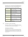
Table 1-1: The seven research divisions at FOI
1.2.1.
The Division of Sensor Technology
The projects in which we have been working mainly involve two
departments in the Division of Sensor Technology: IR Systems and
Laser Systems. A short description can be found below.
The Department of IR Systems
This department focuses on object detection in the thermal IR range,
although they cover other optical ranges as well. This involves issues
concerning different targets, backgrounds and atmospheric conditions. The knowledge can be used, for instance, in mine detection and
warning sensors.
Introduction
3
Computer models of terrain and vehicles with IR textures representing different conditions are used as training data to improve image
processing algorithms for detecting objects in a scene. One important
field of application is reconnaissance using unmanned aerial vehicles, where these algorithms are necessary.
The department has 25 employees, many of them specialised in physics.
The Department of Laser systems
The Department of Laser Systems has around 40 employees working
with detection using laser. Lasers are used to measure distances to
objects, but also velocity and shape, and this information combined
can lead to identification. Laser can be used when sight is limited, as
for instance reconnaissance below the water surface by helicopters. It
is also possible to use laser radar to measure the wind velocity.
The department also develops warning systems that indicate when an
object is subjected to laser beams.
1.2.2.
Projects involved in the development of SceneServer
ISM (Information system for target recognition)
The objective for the ISM project is to cover the whole chain of
object recognition, from the sensors gathering the data to the graphical user interface where the data is presented. An information system
is developed where different methods for classifying objects are to be
demonstrated. The system shall also provide tools to help in the process to determine object types, and a standard language shall be developed for multiple data sources. This language shall also provide
possibilities to combine data from different types of sensors.
SIREOS (Signal processing for moving EO*/IR-sensors)
There is a growing need for support systems that help image analysts
to focus on the relevant parts in the vast data sets produced by modern image sensors. The Sireos project has been financed 2000-2002
*.
Electro Optical
4
Introduction
by FOI with the objective to evaluate the need for, and conduct
research on, improved sensor technology through image analysis and
automated object recognition.
OSS (Optronic Sensor System)
The main goal in Optronic Sensor Systems is to optimise the use of
active and passive sensors in collaboration in order to enhance object
recognition. The approach is to strengthen the competence in object
recognition, identification, multi sensor application, and multi target
tracking with optronic sensor systems and to design and evaluate
algorithms for multi-dimensional sensor systems.
IVS (Intelligent munition)
The object is to examine how multi sensor technology and robot
guidance can be integrated to enhance the precision and the capacity
to strike with appropriate force. Areas of importance are: target sensors (IR, laser, and radar), identification and classification, terminal
guidance, and controllable damage effect.
GV (Gated Viewing)
Gated viewing is a technique that uses laser radar for long-range target observation and recognition. The motivation for this technique is
that conventional electro-optical and infrared imaging systems can
sometimes be limited when it comes to disturbing background,
obscurants or bad weather. With a gated viewing laser radar system
you specify a gate (a range) where the system collects target data and
rejects data out of this range.
2. SceneServer introduction
This chapter is an introduction to the parts that SceneServer consists of. A short section about the 3D models
we have worked with is also included. At the end of the
chapter we present a pre-study with future users.
2.1.
System overview
The system called SceneServer is a software for creating, editing, and
rendering 3D scenes. Its main usage is to assist developers of computer vision algorithms by letting them test their work on images and
other data sent from the application. In the involved projects
[Section 1.2.2], most computer vision algorithms are developed in
MATLAB, hence it is vital that SceneServer can communicate with
that environment.
client
server
Figure 2-1: SceneServer communication architecture
5
6
SceneServer introduction
The SceneServer architecture consists of a MATLAB client using
Java and a server side implemented in C++:
The client side
• SireosLib, a library written in Java by Frans Lundberg. SceneServer
uses a part of this library, the network communication between Java
and C++.
• SceneServerLib, a subclass of SireosLib that handles the particular
commands used with SceneServer.
The server side
• SireosServer, C++ classes which gather the messages sent from SceneServerLib.
• SceneServer Interface, that handles the communication with the scene
graph.
• A Windows application with a Graphical User Interface that presents
the 3D renditions.
The functions in SceneServer can be called from the MATLAB client
through Java, by calling the functions in SceneServerLib directly
from Java, by using the GUI application, and/or by calling functions
in the SceneServer Interface.
2.1.1.
SireosLib
This is the client that connects to SireosServer. The SireosLib library
has been built in Java to enable commands in MATLAB to be sent to
other applications. MATLAB supports Java, but however all versions
but the latest (6.5) only have support for JDK 1.1. After the library is
imported to MATLAB, functions contained in the subclass SceneServerLib can be called and parameters be passed directly from
MATLAB.
2.1.2.
SceneServerLib
This is a subclass to SireosLib and a set of basic functions were
implemented in the prototype available at the beginning of our work
[Section 2.2]. SceneServerLib handles all commands that are communicated between the MATLAB client and SceneServer, but can
also be called directly from a Java class.
SceneServer introduction
2.1.3.
SireosServer
SireosServer consists of a number of C++ classes that handle the
communication with the client. The server receives text strings with
parameters sent through SceneServerLib using the network architecture in SireosLib and calls the appropriate functions in the SceneServer Interface. Parameters or byte arrays are returned to MATLAB
through Java (SceneServerLib).
2.1.4.
SceneServer Interface
The SceneServer Interface consists of cross-platform classes that
contain functions for handling the scene graph, using the scene graph
library OpenSceneGraph (OSG) [Section 3.3].
2.1.5.
The Windows GUI
This application is built using the Microsoft Foundation Classes
(MFC) and thus has the usual Windows look. It renders the 3D scene
and allows the user to interact with the 3D world [Fig. 2-2]. When the
application is executed it also initialises the server.
7
8
SceneServer introduction
Figure 2-2: The Windows GUI
2.2.
The prototype
When we started working on this software, a prototype already
existed which contained some basic functions. It was possible to read
OpenFlight files [Section 2.3], to translate and rotate objects and
camera, and to set values for one light source. The connection from
MATLAB through SireosLib existed, but only included a few functions in the subclass SceneServerLib. The prototype also included a
basic GUI built by Jörgen Ahlberg.
SceneServer introduction
2.3.
Models (OpenFlight)
In the specification for this thesis the main format for models was
specified as the OpenFlight format (.flt) [2]. This is a wide spread
format by MultiGen-Paradigm that has become the de facto standard
in the industry. Open Scene Graph has a plugin to load OpenFlight
models, hence SceneServer can load .flt files. FOI has gathered a collection of military vehicle models to use in visual simulation. In addition, landscape models over the FOI area in Linköping and the
military exercise area called Kvarn have been developed at the Division of Sensor Technology.
2.3.1.
The Kvarn model
The terrain model of the Kvarn area was created from high spatial
resolution data collected using a helicopter carrying a laser measuring system. The system was also equipped with a high-resolution digital camera and an IR camera. The surface model covers an area of
1500 x 1500 metres and has a geometric resolution of 0.25 metres per
pixel. Geometrically corrected image data from the IR camera
[Fig. 2-3], with resolution of 0.2 metres per texel*, has been used to
texturize the model.
From the surface model it is possible to extract information about
vegetation and other objects. This information has been used to position 3D models of trees, with correct size, into the model. In a similar
way, buildings have been automatically constructed using data from
the IR camera as textures.
*.
A pixel in a texture image is commonly called texel.
9
10
SceneServer introduction
Figure 2-3: Assembled IR images showing the Kvarn area
2.4.
Pre-study
In order to define which functions that needed to be implemented in
SceneServer we asked a number of potential users involved in various projects that might use this application. A list with about ten persons from different departments and projects was prepared. Meetings
were arranged where we discussed the features that each individual
ranked as important for their future use of SceneServer, if they
already used the prototype SceneServer, and in what way SceneServer could be of use in later stages.
These interviews resulted in a number of points presented in the following sections. The list does not contain the basic functions such as
loading object models, rotating objects and so on. The functions are
grouped in different priority levels, where A has the highest priority.
SceneServer introduction
2.4.1.
11
Group A - high priority
Level of detail
Adjust the level of detail for the objects in a scene.
In this application the quality of the rendered images is of greater
importance than the workload of the system. Therefore the initial
level of detail settings must be discarded to secure a high quality
image to run the computer vision algorithms on.
Dynamic textures
Change the texture on an object dynamically.
It should be possible to change the texture on an object in order to
adjust the object’s appearance to better coincide with the surroundings. It is important to be able to fine-tune the object's IR signature.
Scene graph
Visualise the tree structure of a scene.
There should be a way to view the structure of the scene graph. This
is useful because it gives the user information about the structure of
the objects in the scene and what sub parts the objects are divided
into.
Camera settings
Change perspective, focal length, and alter the screen size.
The user must be able to adjust the camera according to the specific
task at hand. The camera should support both perspective and orthographic projection.
Articulate parts
A method to select different parts of an object to articulate.
It is vital that the objects subjected to object recognition algorithms
could vary in different degrees of freedom. Hence, it must be possible to articulate an object’s sub parts.
12
SceneServer introduction
2.4.2.
Group B - medium priority
Depth buffer
Retrieve information about the depth in a rendered image.
The information in the graphics card's depth buffer should be sent to
MATLAB, converted so that each pixel in the current image is translated into a value that corresponds to the distance from the camera to
the pixel. This would simulate the use of a laser radar.
Log scene activity
Collect all parameters affecting the scene and store them in a file.
This is useful because a scene can be restored to a previous state if
something goes wrong or if the test for some reason needs to be
expanded or reconstructed.
Generate textures
Extract a texture image from the area occluded by an object.
The extracted image could be used to texturize the object. This is
useful in matching algorithms, to evaluate the probability of a correct match of a test object.
Data to MATLAB
Returning information from SceneServer to MATLAB.
Returning information, for instance rendered images, directly to
MATLAB without having to store it on the hard drive. This saves
time and resources.
Tripod and paths
Place objects at ground level and define checkpoints to build paths.
It should be possible to calculate the position and rotation of an
object in correspondence to another object, such as a landscape. If a
set of checkpoints could be defined in the GUI, paths in the scene
could be calculated and objects be assigned routes to follow.
SceneServer introduction
Navigation
2.4.3.
13
Navigating the scene in the GUI.
There is a need for a way of navigating in the scene using the keyboard or the mouse. This gives the user a way to preview the scene
and specify areas of importance.
Group C - low priority
Dynamic selection
Define which objects that are currently visible.
If objects dynamically could be loaded into, or removed from, the
scene graph it would decrease the workload on the system by freeing
memory resources.
Small objects
Rendering objects smaller than a pixel.
In most graphic systems objects smaller than a pixel are discarded.
When designing algorithms that detect, for instance, incoming
objects (i.e. missiles) every split second is vital. Hence, the lost
information because of small objects is valuable and must be taken
into account.
Vertex lists
A standard method for describing the objects in matrix lists.
If one could retrieve generated lists in MATLAB and assemble
objects from lists in MATLAB, the user would have total control of
the objects in a scene, allowing changes to be made in order to
secure that the objects/models correspond with reality.
Cameo-Sim
Assure that Cameo-Sim can handle the same models as SceneServer.
By using a general file format for the objects used by SceneServer
the data could be exported and imported to different tools allowing
the user to take advantage of the different specialities of the applications. Cameo-Sim is a software from InSys Ltd solving various
forms of the radiation transport equation, including atmospheric,
radiative and heat-transfer in natural scenes.
14
SceneServer introduction
Light source
Synchronize the light source with the time of day.
This would be an easy way to control the light source (sun).
Collision detection
Detect collisions of objects in the scene.
If one could find a method for collision detection, preferably without
using the depth buffer which depends on the resolution, this would
assure that the objects are placed correctly.
Shadows
Shadow casting from objects.
This function needs to be implemented in order to gain a more accurate visualisation of the scene.
Covered areas
Extract information on which area that is covered by the camera.
This function could be used to evaluate the accuracy of coverage
algorithms that calculate the camera positions needed to cover a
desired area.
3. Background technologies
In this chapter the 3D graphic technologies used in this
project are described. There are short sections on
OpenGL and scene graphs in general, and a more thorough section on Open Scene Graph.
3.1.
OpenGL
OpenGL [3][4] is a software interface for creating advanced computer graphics in 2D and 3D. In OpenGL, 3D objects are built by using
geometric primitives such as lines, triangles, and polygons. It is possible to arrange your objects in the 3D world and to set up a viewing
plane with a chosen projection type. Colours are calculated based on
specified primitive colours, lighting conditions and textures. Before
the scene is rasterized, i.e., the mathematical description of the
objects and their attributes are converted to pixels on the screen, hidden surface removal could be done using a depth buffer.
3.2.
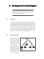
Scene graphs
A scene graph is a tree Root node
structure of data that
stores and organises
scene information such as
objects, appearances, and
materials [5]. In other
words, putting your data
into a scene graph is a
way to structure your
graphical data in a scene.
The scene is arranged as
a structured graph with
Leaf node
different types of nodes Figure 3-1: Scene graph structure
that are linked, usually in
an acyclic manner, i.e.
15
16
Background technologies
there are no links from a node to any of its predecessors or to a neighbouring branch [Fig. 3-1]. If such links were to occur the traversal of
the graph would create infinite loops.
The scene is built from a single root node, which contains children
that are the objects/models in the scene. The figure above [Fig. 3-1]
describes a scene with two objects; the objects are represented by sub
trees that host different types of nodes. A scene graph node can be
either a group node or a leaf node. Some typical sub-types are:
Group nodes
• Group: A node to group a subset of children.
• Switch: Acts as a switch to activate different parts of the tree under
defined conditions.
• Transform: This node transforms the geometries in its children.
• Level of detail (LOD): A node that contains a range for each child,
and displays the children if the range coincides with their distance to
the camera.
Leaf nodes
• Geometry: Basic container for the geometry primitives in the object.
3.3.
Open Scene Graph
Open Scene Graph (OSG) [6] is an open source cross-platform scene
graph library for visualisation of real-time graphics, and requires
nothing more than OpenGL and standard C++. OSG is currently in
beta stage, working towards version 1.0 with Robert Osfield as
project lead.
OSG is far from the only scene graph library on the market, and has
both benefits and drawbacks compared to its competitors. The largest
disadvantage is that OSG lacks any documentation but that created
automatically by Doxygen, which contains only sparse comments.
Another problem is that OSG changes frequently because of the beta
stage. Updates need to be made continuously to fix new bugs, and as
a developer you always have to keep an eye on the mailing list. All
this should get better when the development reaches version 1.0.
The fact that OSG is open source is of course an advantage, both that
it is free to use and that you have the option to read and modify the
code if needed. OSG also comes with some nice demos, which at
Background technologies
17
least to some extent compensate for the lack of documentation. You
do not have to wait for long to get an answer on the mailing list
either. Another reason why OSG was chosen in our project is that it
includes readers for many image and 3D model formats; most importantly for us is the support of the OpenFlight format.
A book on Open Scene Graph based on OSG 1.0 will hopefully be
released in late 2003.
3.3.1.
Scene graph structure in OSG
The root in an OSG scene graph is a Group node [Section 3.2].
Below the root, the tree is built using more Group nodes and/or
Transform, LOD and Switch nodes. The leaf nodes in OSG can be
Geodes or Billboards and they contain a number of Drawables, which
is the base class in OSG for all kinds of geometries. A Billboard is
just a Geode that orientates its child to face the eye point.
Group
StateSets
Groups, Transforms, LOD’s Switches
Geodes, Billboards
Nodes
Drawables
Figure 3-2: OSG scene graph structure
All nodes, except the leaf nodes, and the Drawables can have a connected StateSet, a class that encapsulates the OpenGL state modes
and attributes [Fig. 3-2]. This can for example be texture and material
attributes in the case of a Drawable.
3.3.2.
Viewing the scene
To view the scene, a SceneView class is used. This class contains a
pointer to the whole scene graph, but also a camera, light and the global states, such as fog settings.
18
3.3.3.
Background technologies
Editing the scene graph using Visitors
The concept of Visitors is widely used in programming and an important part of OSG. The Visitors in OSG are based on the GoF design
pattern [7].
The idea in OSG is that you traverse a part of the scene graph with a
Visitor object, making it possible to modify desired nodes. All types
of nodes have accept() methods for OSG's NodeVistor. A little simplified they look like this:
void Node::accept(NodeVisitor& nv)
{
nv.apply(*this);
}
A Visitor can be used to modify more than one node in a subgraph by
calling traverse() in the subgraph’s root node:
myGroupRoot->traverse(*myVisitor);
The function traverse() calls accept() in all the node’s children with
the Visitor as argument.
In myVisitor there should be apply() methods for all types of nodes
the Visitor is supposed to affect. When a node's accept() method is
invoked after the traverse() call, the correct apply() method in
myVisitor will be called. Inside this method the node can be altered.
For instance, a Visitor for modifying every Geode in an object could
look like this:
class GeodeVisitor : public osg::NodeVisitor
{
public :
GeodeVisitor() : osg::NodeVisitor( TRAVERSE_ALL_CHILDREN )
{ }
virtual void apply( osg::Geode &geode )
{
//modify the Geode here
}
virtual void apply( osg::Node &node )
{
//if the node is not a Geode, continue to all its children
traverse(node);
}
}
This Visitor could then be used like:
GeodeVisitor *geodeVis = new GeodeVisitor();
//traverse the selected child
_sceneGraphRoot->getChild( objectNumber )->traverse(*geodeVis);
With this technique, type safe modifications can be done on all different types of nodes in OSG.
4. Implementation
In this chapter we describe the different classes in the
SceneServer architecture in more detail. There is also a
section covering the implemented functions.
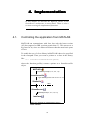
4.1.
Controlling the application from MATLAB
MATLAB can communicate with Java, but only the latest version
(6.5) has support for JDK versions greater than 1.1. This was never a
big issue for us, since we did not need more than the most basic parts
of Java.
To enable the use of a Java library in MATLAB it has to be specified
in the classpath. Then you create a pointer to a class in the library
like:
ss = sireoslib.SceneServerLib.getLib;
where the function getLib() returns a pointer to a SceneServerLib
object.
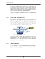
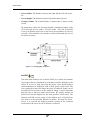
MATLAB
ss.setBackground(0.7, 0.7, 0.2, 1.0)
SceneServerLib
“-type setBackground -color 0.7 0.7 0.2 1.0”
SireosLib
client
server
SireosServer
setBackground(0.7, 0.7, 0.2, 1.0)
Interface
Figure 4-1: Example of communication using a
MATLAB client
19
20
Implementation
Now, calls to functions in SceneServerLib, like:
ss.setBackground(0.7,0.7,0.2,1.0);
can be made. This call is assembled in SceneServerLib to a string
with parameters, "-type setBackground -color 0.7 0.7 0.2 1.0", which
is sent to the server. When arriving to the C++ server class, the type
of command is checked, the correct function in the SceneServer
Interface is called and the appropriate changes in the scene graph are
made [Fig. 4-1]. Another string of the same type as above is sent
back to Java containing a status message and in some cases one or
more variables which should be returned to MATLAB.
4.1.1.
Examples of using SceneServer from MATLAB
In this section two examples of communicating with SceneServer
from a MATLAB client are shown. The code is commented and all
functions used are explained in more detail in Section 4.3 and Appendix A.
Implementation
21
Example 1: Sending vertices to MATLAB
%Get access to the functions in the Java class
%SceneServerLib.
ss = sireoslib.SceneServerLib.getLib;
%Read an object specifying an object name (myObject) and
%translation (0,0,0).
ss.readObject('C:\models\myObject.flt', 0, 0, 0, 'myObject');
%Edit an object part named 'Turret'
%'myObject'. Rotation (0.5 radians)
%in the local coordinate system for
ss.editPart('myObject','Turret', 0,
in the object
around z-axis
the object part.
0, 0.5);
%Get a transformed vertex list from the object.
vertexList = ss.getVertexList('myObject');
%Create a face-list
faceList = reshape([1:(size(vertexList,1))], 3, (size(vertexList,
1))/3)';
%View in MATLAB using MATLAB's trimesh function.
%trimesh(TRI,X,Y,Z,C) displays the triangles defined in
%the M-by-3 face matrix TRI as a mesh. A row of TRI
%contains indexes into the X,Y, and Z vertex
%vectors to define a single triangular face.
trimesh(faceList, vertexList(:, 1), vertexList(:, 2),
vertexList(:, 3));axis equal;
Figure 4-2: The resulting MATLAB trimesh
figure from example 1
22
Implementation
Example 2: Images and depth buffers
%Get access to the functions in the Java class
%SceneServerLib.
ss = sireoslib.SceneServerLib.getLib;
%Read a landscape model without specifying any transform
ss.readScene('C:\models\scene.osg', 'landscape');
x = 930;
y= 1320;
%Read a vehicle and place it into the scene at
%(x,y,z)=(930,1320,0)
ss.readObject('C:\models\tank.flt', x, y, 0, 'myVehicle');
%Place the vehicle correctly rotated on the ground at
%(x,y) = (930,1320) with z-rotation 1.8 radians.
ss.tripod('myVehicle', x, y, 1.8, 0.8, 1.0, 0.1);
%Set the camera properties
ss.setLookAt(x-17, y+39, 74, x+6, y-10, 63, 0, 0, 1);
fovy = 20; %Field of view in degrees
%Set a perspective projection
ss.setPerspective (fovy, 400, 300);
%Set a distance for the highest level of detail
ss.setLOD(1000);
%set light
ss.setLight(0, 0, 1, 0, 1, 1, 1, 1, 1, 1, 1, 1, 1, 1, 1, 1);
i = ss.getDoubleImage; %get image data
height = ss.getHeight; %get image height
width = ss.getWidth; %get image width
image = zeros(height,width,3);
%reshape image
image(:,:,1) = reshape(i(1:3:length(i)),width,height)';
image(:,:,2) = reshape(i(2:3:length(i)),width,height)';
image(:,:,3) = reshape(i(3:3:length(i)),width,height)';
figure;
imshow(image);
depth = ss.getDepthBuffer; %get depth buffer data
depth = depth./max(max(depth)); %re-scale
figure;
imshow(depth);
Figure 4-3: Resulting images from example 2 displayed in MATLAB. To the
left the image from SceneServer, to the right a depth buffer image.
Implementation
4.2.
23
The server side part of SceneServer
Visitors
Interface
SireosServer
Connecting
Java and the
C++ application
Document
For editing
nodes in the
scene graph
View
OpenGLWnd
Dialogs
SceneGraphDoc
For user input
in the application
SceneGraphView
SceneGraphWinApp
MFC startup class
Cross-platform
inheritance
Windows specific
pointer
Figure 4-4: C++ structure
4.2.1.
The SireosServer classes
As mentioned earlier, the server classes handle the connection with
the Java library SireosLib [Section 2.1.1]. The classes were implemented in both a Windows and a Unix version before we began our
work. We have edited a subclass to the Windows server that manages
the connection with the C++ SceneServer Interface. This class should
also be able to inherit the Unix server and thus be used in a possible
Unix version of SceneServer.
SireosServer recieves a string with a number of parameters. The type
of command is checked, all parameters are read, and the appropriate
function in the Interface class is called using the subclass mentioned
above. A status message is always returned, reporting if the operation
could be performed. In some cases parameters are returned to SceneServerLib [Section 2.1.2], either as a string or as a byte array.
24
4.2.2.
Implementation
The cross-platform part
The part of SceneServer using OSG is cross-platform and therefore it
could be re-used if the application should be implemented in another
operating system. The basic class here is the Interface, a Singleton
class [7] containing all functions that can be called from the client
and/or from the GUI. A Singleton class is a class that can have one
instance only. The constructor is private and the instance can only be
accessed by using the instance() method.
Interface* Interface::instance()
{
if( _instance == 0 ) // is this the first call?
{
_instance = new Interface; // create sole instance
}
return _instance; // return address of sole instance
}
The Interface class contains pointers to a Document and a View
object. Every function in the Interface just calls a function with the
same name and parameters in either one of these objects. Dividing
functions into a Document and a View class is a common design pattern [7], well supported by MFC [Section 4.2.3] and OSG. The View
class handles changes to the graphical elements, while the Document
class stores and handles all data. In our case, the View class takes
care of changes in the camera settings and general viewport
attributes, such as fog. It also includes functions for reading images
and depth buffers. Here we have access to the SceneView object. The
Document class has functions for reading objects and editing the
scene graph, and therefore it has a pointer to the scene graph root.
We also have a number of Visitor classes [Section 3.3.3] for editing
the scene graph:
• LODVisitor: For changing the level of detail in a scene.
• TransformVisitor: For transforming object parts.
• TreeVisitor: For collecting the scene graph structure in a vector string
that can be used to print the structure in MATLAB or display it in the
GUI.
• GeodeVisitor: For changing an object’s texture.
• VertexVisitor: For editing vertex, texture, and colour lists.
All these Visitors extend OSG's NodeVisitor [Section 3.3.3].
Implementation
4.2.3.
25
The Windows specific classes
All classes that handle the Windows GUI are collected in their own
namespace. If the system should be implemented in, for example,
Unix only these classes need to be re-implemented. The GUI is built
in Visual C++ using MFC (Microsoft Foundation Classes) [8].
MFC supplies a framework with four main classes to help users begin
with a project. The first two are a main application class and a main
frame, the latter representing the outer main window frame including
menus. In our application, these classes are called SceneGraphWinApp and MainFrm. SceneGraphWinApp inherits the MFC class
CWinApp. The other two classes in the framework are representing
the Document/View architecture and inherit the MFC classes CDoc
and CView; in our case they are named SceneGraphDoc and
SceneGraphView. These classes take care of events from the GUI,
and call the proper functions in the Document or View class.
SceneGraphDoc handles events that should trigger functions in the
Document class, and therefore extends this class. SceneGraphView
works in a similar way, inheriting the View class. This class must,
for example, have a method for changing the window size, because
this function is needed when changing projections but can not be
implemented in a cross-platform class. These kinds of functions are
virtual functions in the View class, and are implemented in
SceneGraphView.
To be able to use OpenGL together with MFC, SceneGraphView also
inherits a class called OpenGLWnd. This class handles the OpenGL
initiations needed.
Finally, there are ten Dialog classes that map a number of variables
with the user input from the GUI.
4.3.
Implemented functions
Most of the functions we have implemented can be accessed both
from the MATLAB client and the GUI. In the description below we
use the following two icons to illustrate where these commands can
be used:
represents MATLAB functions and
represents GUI
functions.
26
Implementation
The descriptions are divided into six categories:
• General functions
• Camera and viewport settings
• Read, edit and save objects
• Read and write images
• Image depth and intersection
• Scene graph manipulation from MATLAB
4.3.1.
General functions
These functions are not manipulating the scene graph.
setIP
It is possible to control SceneServer from another computer than the
one running the SceneServer GUI application, by specifying the
other computer's IP number.
Save as MATLAB-file
During the pre-study a need to save a complete scene with all information gathered in some way was expressed. Since the scene manipulation in SceneServer can be done both from MATLAB and the GUI
we found that the most efficient way to save all information was to
log the commands. Every executed command is logged in an array of
strings. Some of the commands, like changing the camera position,
are overwritten in the array, and when an object is deleted all earlier
commands relating to this object are removed.
This is very efficient in the sense that a whole scene can be set up and
saved with only some kilobytes of MATLAB command code. If the
user then wants to reconstruct the scene, he runs the script file from
MATLAB and SceneServer reconstructs the scene command for
command, hence it is possible to save the current state in the application.
Implementation
27
Navigation
The user can move and rotate the camera in the application by using
the keyboard. It is also possible to get an overview of the scene; the
camera position is then calculated using the whole scene's bounding
sphere. This can be useful if the user is uncertain where in the 3D
space an object has been placed, or to scout a scene to find areas of
interest.
4.3.2.
Camera and viewport settings
This segment covers functions that manipulate the camera in the
scene and the overall appearance of the scene.
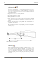
setLookAt
This function orientates the camera and specifies the locations of the
camera and the center point. The parameters are eye(x,y,z),
center(x,y,z) and up(x,y,z) [Fig. 4-5]. Eye specifies the position in
space of the virtual camera, center sets the center point at which the
camera is pointing. The third parameter, up, specifies the orientation
of the local coordinate system in which the camera is positioned,
hence up controls the orientation of the camera.
Figure 4-5: Camera parameters
28
Implementation
setPerspective
Perspective projection [9] is the default projection type in SceneServer and this projection type is designed to describe the world similar to how a camera or our eyes perceive it. This projection has the
following parameters:
• fovy: Field of view in the screen y direction.
• w: Width of the screen in pixels.
• h: Height of the screen in pixels.
• near: The distance when the camera starts displaying objects, anything
closer than the near plane will not be shown on the screen. The unit is
metres.
• far: The far cutting plane, anything farther than this will not be displayed. The unit is metres.
By setting these parameters you specify the perspective viewing frustum [Fig. 4-6].
Figure 4-6: Perspective projection
setOrtho
When using orthographic projection [9] the distance from an object
to the camera does not affect how large the object appears on the
screen. The viewing volume is a box and this projection type is used
when it is important to maintain the size of objects and the angles
undistorted by the perspective [Fig. 4-7]. The following parameters
can be set:
Implementation
29
• Screen width: The distance between the right and the left side in pixels.
• Screen height: The distance between top and bottom in pixels.
• Viewport width: The actual distance in metres that is shown on the
screen.
By using these values the Viewport height is calculated simply using
( Screen height ⁄ Screen width ) ⋅ Viewport width . Then the projection
is set up so that the pixel size on the screen corresponds to a real size
in metres. This function is for instance useful to determine the size of
an object in metres.
Figure 4-7: Orthographic projection
setLOD
The main idea behind level of detail (LOD) is to reduce the number
of polygons that are displayed in accordance with the distance to the
object. If you are a long way from the object a less detailed object
could sometimes be displayed with a fairly good visual result. The
fewer polygons to draw the faster the scene is rendered. In the case of
SceneServer the accuracy of the rendered image is more important
than the time it takes to render each frame. We simply discard all
detail levels but the highest for the best possible visual result. The
function setLOD sets the range of the highest level of detail from
zero metres to the specified distance in metres. The goal for SceneServer is to provide the highest possible quality of the rendered
scenes hence the lower levels of detail are removed.
30
Implementation
The picture below [Fig. 4-8] shows a model and its different levels of
detail. In this case you would use a less detailed version of the bunny
when it is far from the camera. However, if you were to import this
model to SceneServer only the highest level of detail would be used
at all times and distances up to the distance you set with this function.
Figure 4-8: Example of different level of details
osgComputeNearFar
SceneServer has through Open Scene Graph the default setting that
OSG computes the near/far cutting planes every time the view is
updated. This is done by calculating a bounding box* over all objects
in the scene. This can be overridden by specifying the near/far cutting
planes in setPerspective
setLight
The light that affects the scene is set up in the SceneView as a
SKY_LIGHT (the position of the light source is fixed, independent
of the camera position and rotation). This mode is used in SceneServer to simulate a single light source and the function setLight
specifies the position and colour of this light source.
setBackground
This function served as an excellent start to get a grip of the prototype SceneServer structure and it simply changes the colour of the
background in the scene.
*.
A box that envelopes the object.
Implementation
31
setFog
The fog class in OSG encapsulates the OpenGL fog state [3]. Fog is a
term for several types of atmospheric effects like smoke, haze, mist
or other types of effects that degrade the visibility. This is used to
create a more realistic simulation of the virtual environment. There
are three different types of equations that can be used to create the
fog effect (1)(2)(3). The main idea is that objects farther away from
the viewpoint begin to fade into a specified fog colour.
end – z
f = --------------------------end – start
f = e
f = e
– ( density ⋅ z )
– ( density ⋅ z )
(GL_LINEAR)
(1)
(GL_EXP)
(2)
(GL_EXP2)
(3)
2
The GL_LINEAR equation is in our opinion not very useful, hence
we included GL_EXP and GL_EXP2 in SceneServer. The parameters
to set in setFog is:
• Density: Determines how dense the fog is, i.e. how fast the fog is
affecting the scene in regard to the distance from the viewpoint.
• Colour: The colour of the fog effect.
• Mode: Sets the GL_EXP or GL_EXP2 fog mode.
The picture below [Fig. 4-9] describes how the different fog modes
behave.
Figure 4-9: Fog modes
32
Implementation
autoUpdateView
SceneServer has a default setting of auto updating the screen after
each function is called. There are however many situations when you
do not want this to happen at every step in a series of commands. By
setting autoUpdateView to zero you turn off the auto update, and you
can specify exactly when to update by using updateView.
updateView
This function updates the viewport when called. If the automatic
update is turned off then this is the function to call to render the
scene. This is necessary when you for instance want to set up a scene
with a number of objects and then manipulate several objects before
rendering the scene. You would not want the scene to re-render after
each command causing SceneServer to render unnecessary steps.
4.3.3.
Read, edit and save objects
The functions in this section manipulate objects and handle the
import/export of models.
readObject
Objects can be loaded both from MATLAB and from the GUI. The
model types supported in SceneServer are those supported by the
OSG loaders, for example OpenFlight, 3Dstudio, SGI Performer, and
the format native to OSG. When the objects are loaded they can also
be placed as desired in the scene by specifying translations, rotations
and scaling. All these transformations are stored in a transformation
matrix placed above each object's root node in the scene graph.
Objects in SceneServer can also be given names. These names can
then be used to specify an object when edited from MATLAB. They
are also displayed in a Dialog when an object should be edited or
deleted from the GUI [Fig. 4-10].
Implementation
33
Figure 4-10: Choosing an object in the
GUI
editObject
This function is used to edit an object's transformation matrix, i.e. to
move, rotate and scale the whole object. To ensure that we get the
right lighting calculations on an object, we turn on the OpenGL
attribute GL_NORMALIZE [3]. Otherwise, the lighting can be miscalculated if the object is scaled.
saveObjectAsOSG
The current OpenFlight loader in OSG has a local cache memory to
ensure that OpenFlight models that are loaded can be instanced if
they are attempted to be loaded a second time. Since this local cache
can not currently be manually flushed to free memory, we have
included a function in SceneServer to save objects in OSG's own format. This will be changed in an upcoming version of OSG, but until
then OpenFlight models must be converted into the OSG format if
memory should be freed when they are deleted in SceneServer.
viewSceneGraph
The whole scene graph can be viewed both from MATLAB and from
the GUI [Fig. 4-11]. The node types and the structure of the scene
graph are displayed. If the nodes have names, which is common for
most nodes in an OpenFlight model, they are shown as well.
34
Implementation
Figure 4-11: View scene graph in MATLAB and GUI
The information that can be seen here is useful when different parts
of an object, and not the whole object, should be edited. As mentioned earlier, the application can be run on a different computer than
the one controlling it from MATLAB, and therefore the information
can be accessed from MATLAB, and not only from the GUI.
editPart
Different parts of an object can be transformed in SceneServer
[Fig. 4-12]. They can be translated and scaled, but most importantly,
they can be rotated around their local origin. This function is currently adapted to the OpenFlight models we have worked with that
have DOFTransforms* for every part that should be able to be transformed.
The function is used from MATLAB by specifying the name of the
object and the part, how much the part should be rotated and, if
desired, how much it should be translated and scaled. The part names
available in an object can be seen by viewing the scene graph in the
application or from MATLAB.
*. A degree-of-freedom (DOF) node serves as a local coordinate system. It specifies the articulation of parts in the model
and sets limits on the motion of those parts.
Implementation
35
The possibility to make these changes is useful because identification
algorithms can then be tested on objects with different articulation.
When an object’s vertex list is sent to MATLAB [Section 4.3.6],
these transformations are included.
Figure 4-12: Rotation of turret
clear
, deleteObject
, and deletePart
With these commands, the whole scene graph can be cleared, one
object can be removed or one specified node in the scene graph can
be deleted. As mentioned above, deleting objects loaded from OpenFlight files do not free memory (see saveObjectAsOSG), they have to
be converted into OSG's own format first.
The deletePart function gives the user the possibility to remove undesired parts of an object.
36
Implementation
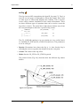
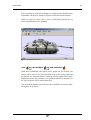
tripod
This function is used to align objects to the ground. Since the users of
SceneServer work with identification of ground vehicles, it is useful
to have a function that automatically places objects correctly rotated
on the ground level. The user only has to specify the x and y coordinates and the forward direction [Fig. 4-13].
Figure 4-13: Using the tripod in the GUI
We use four points to compute the object's new forward, left and up
vectors [Fig. 4-14]. P1-P2 gives the left vector while P4-P3 is the forward vector. The up vector is calculated by taking the cross product
of these vectors.
Figure 4-14: Tripod information
The default placement, in the xy plane, of the points is calculated
using the object's bounding box, but can also be decided by the user.
The z-value of the points is computed using the same technique as in
getIntersection [Section 4.3.5], by sending beams orthogonal to the
xy-plane. The object itself is masked during this step, so we only get
hits on other objects. Since we have no flying objects in our application, we do not care which object we get the first hit on. Otherwise,
the user would have to specify which objects that should be counted
as ground elements.
Implementation
37
At first we send beams distanced by 2 ⋅ step_x and 2 ⋅ step_y . Then
we have to re-calculate the x and y values because of the problem
shown in the figure below [Fig. 4-15]; since the ground is tilting the
actual step in the x direction is x_error . The angle alpha can be used
to compute a new step length (4), assuming that the angle would
remain the same.
Of course, this is just an approximation, but it could be used in a
number of iterations to get a good result.
Figure 4-15: Errorous step
length
new_step = step_x ⋅ cos ( asin ( ( ∆h ) ⁄ P1 – P2 ) )
Calculation of new step length
(4)
The resulting vectors can then be used as row vectors in the transform matrix. But since the users need to know the rotation angles of
an object, we have to be able to return these to MATLAB. Thus, they
are calculated using a conversion to Euler angles [10]. Euler angles,
commonly named head, pitch and roll, are easy to understand, but
they do have drawbacks. To extract them from an arbitrary transform
matrix is somewhat troublesome. Firstly, the angles depend on the
order of rotation (actually, there are 24 different ways to form an
Euler Transform [11]), secondly, there is not always a unique solution.
An Euler Transform can be written: R = R x ( θ x )R y ( θ y )R z ( θ z )
using three rotation matrices, one for each axis (5). The ordering we
use is xyz.
38
Implementation
cos θ 0 sin θ
1 0
0
R x ( θ ) = 0 cos θ – sin θ R y ( θ ) =
0 1 0 Rz( θ) =
0 sin θ cos θ
– sin θ 0 cos θ
Rotation matrices
cos θ – sin θ 0
sin θ cos θ 0
0
0 1
(5)
Multiplying, setting R = [ r ij ] for 0 ≤ i ≤ 2 and 0 ≤ j ≤ 2 and using
the notation c i = cos ( θ i ) and s i = sin ( θ i ) for i = x, y, z , yields:
r 00
r 10
r 20
r 01
r 11
r 21
r 02
cycz
=
r 12
czsxsy + cxsz
r 22
– cxczsy + sxsz
–c y s z
sy
c x c z – s x s y s z –c y s x
czsx + cxsysz cxcy
At first we see that s y = r 02 , and therefore θ y = asin ( r 02 ) . If
θ y ∈ (– π ⁄ 2,π ⁄ 2) , then c y ≠ 0 and c y (s x,c x) = (– r 12,r 22) in which
case θ x = atan 2 (– r 12,r 22) . Similarly, θ z = atan 2 (– r 01,r 00) .
This will be true in our case since we will not have rotations of 90
degrees or more around neither the y-axis or the x-axis. If
θ y ∈ {π ⁄ 2, – π ⁄ 2} it can be shown that the factorization is not
unique.
Thus:
 θ x = atan 2 (– r 12,r 22)

 θ y = asin ( r 02 )

 θ z = atan 2 (– r 01,r 00)
Euler angles
(6)
The main reason why we wanted to use Euler angles is that they are
easier for the user to work with when editing an object. The alternative would be to use quaternions [11], that are superior to both Euler
angles and matrices when it comes to rotations and orientations.
When using quaternions though, you work with one angle and one
rotational axis, instead of three angles.
To get the result more realistic, the user can also specify how much
the vehicle should sink into the ground.
The function we have implemented, using four points to calculate the
transform, could of course be more advanced to gain a higher accuracy, but it works fine for this application.
Implementation
39
Figure 4-16: Tripod demonstration
setTexture
When working with IR textured models, it is very important that the
texture can be edited to match different conditions. This function lets
the user change the current texture of an object by replacing it with a
new texture image. IR textures are affected by heat instead of light,
so the only way of changing the appearance of the texture in SceneServer is to manually replace it.
Figure 4-17: IR textures based on different conditions
4.3.4.
Read and write images
These functions handle the image data.
40
Implementation
getImage
and getDoubleImage
The last rendered image can be sent directly to MATLAB as an array.
At first the image data is read from the graphics card to the memory
using the OSG function readPixels, which in turn uses OpenGL's
glReadPixels [3]. The data is then sent as a byte array to the client.
_image->readPixels( viewport_x, viewport_y,
viewport_width, viewport_height, GL_RGB,
GL_UNSIGNED_BYTE );
GL_RGB and GL_UNSIGNED_BYTE are OpenGL constants specifying the data that should be read and the data type of each element.
The data is returned to MATLAB as a byte (getImage) or double (getDoubleImage) array. In the latter case, the data is converted in SceneServerLib. Reformatting the data to a three dimensional matrix
(R,G,B) could be done in Java, but MATLAB's reshape function* is
much faster.
writeImageFile
The last rendered image can be stored as a BMP (bitmap) file. This
command can be accessed both from MATLAB and from the GUI
and it is an easy way to save an interesting screenshot. If the image
data should be processed directly in MATLAB, it is more convenient
to use the function getImage.
For writing images we use an existing writer in OSG.
4.3.5.
Image depth and intersection
The functions in this section simulate laser radar data.
getDepthBuffer
The current depth buffer can be read using readPixels (see getImage)
using GL_DEPTH_COMPONENT instead of GL_RGB.
*.
RESHAPE(X,M,N) returns the M-by-N matrix whose elements are taken columnwise from X.
Implementation
41
The depth buffer data can be very useful information for people
working with identification algorithms, especially for those working
with laser systems, since it simulates data from a laser radar. For
instance, storing depth buffers from different orthographic views of
an object can give a simple, but quite good, description of it [Fig. 418].
Figure 4-18: Depth buffers front/above
To be able to use the depth buffer from OpenGL, the values have to
be re-scaled to represent the distance from the camera in metres. This
can be done using the following equations:
Orthographic projection
(7)
z' = z ⋅ ( z far – z near ) + z near
z near ⋅ z far
z' = ---------------------------------------------------------z far – z ⋅ ( z far – z near )
Perspective projection
(8)
where z near and z far are the distances to the near and far cutting
plane (see setPerspective and setOrtho in Section 4.3.2).
Since the depth buffer levels are spread differently for orthographic
and perspective projections, two equations are needed. When using
orthographic projection the levels are placed linearly from the near to
the far cutting plane, while for perspective projection the levels are
more tightly placed close to the camera than farther away.
getIntersection
This function gives the first intersection coordinates along a line
between two points in 3D space defined by the user. It uses a Visitor
class [Section 3.3.3] in OSG called IntersectVisitor, which can
traverse a scene graph and collect all intersection coordinates in a
vector. The same technique is also used within the tripod function to
calculate where to place the object (see the tripod function), and it
would be the first step towards collision detection.
42
Implementation
This function returns more exact depth data than getDepthBuffer,
since the latter function depends on the number of bits in the depth
buffer.
getObjectIntersection
This function differs from the function above in that it only calculates
intersections with one specified object.
4.3.6.
Scene Graph manipulation from MATLAB
During the pre-study the question was raised regarding some way to
manipulate the objects in detail, i.e. down to the location of each vertex in an object. In order to try to meet these demands we created a
set of functions to extract, manipulate, and create objects from vertex
and face lists.
createObject
Create an object with a transform node, and an empty Geode
[Section 3.3.1]. The transform can be edited by using editPart(). The
Geode is a container for geometries, i.e. vertex lists, face lists, texture
lists, and so on.
addChild
Add a child node of type Geode (for storing geometries) or transform.
setVertexList
Set the vertex list in a specified Geode. The vertex lists can be
arranged as a set of triangles or quads [3].
Implementation
43
getVertexList
Get an object's vertex list in triangles. The vertex list is computed
from the current articulation of the object. An object is often built
from a range of different geometry primitive types like triangles, triangle strips, triangle fans, quads, quad strips and so on. When you
use getVertexList a Visitor [Section 3.3.3] visits all Geodes in the
object and transforms the vertices to triangles regardless of what
primitive type the geometry originally is built from. We do not perform checks on multiple appearances of a vertex point hence the vertex list will in most cases contain duplicate vertices. The face list to a
vertex list extracted with getVertexList is simply an array from zero
to the number of vertices. This is not ideal due to the duplicate vertices, but it works with MATLAB functions such as trimesh (see example 1 in section 4.1.1).
Figure 4-19: Vertex lists shown in MATLAB using the two different modes in getVertexList
The vertex list that we extract from the object can be arranged in two
modes. The first mode takes the part transforms into account when
the vertex list is produced, the second uses both part and object transforms to calculate the vertices [Fig. 4-19]. By multiplying the vertices in every sub tree of the object with the transform matrix for that
part during a traversal the vertices are transformed accordingly.
When leaving a sub tree the inverse transform matrix is multiplied
leaving other parts of the scene graph unaffected.
44
Implementation
setVertexColorList
This function can either set all vertices in an object to a single colour
or if you provide a colour list with a set of colours matching the
number of vertices then the object is coloured in such a way.
setVertexTextureList
In order to add a texture to an object you need to specify which points
on a texture image should correspond to each face on the object. The
width and height of a texture image, not including the optional border
of one texel, must be a power of 2. The texture coordinates are
defined as seen in the figure below [Fig. 4-20].
Figure 4-20: Texture image
The texture list with coordinates is arranged in counter clockwise
order, so if you for instance want to place this texture on a single
quad face the texture list is [0 1; 0 0; 1 0; 1 1]. The orientation of the
texture is determined by the first coordinate for every textured face.
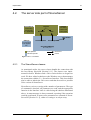
5. Examples of how SceneServer
is used
This chapter contains two examples of how SceneServer
has been used by researchers at FOI.
During the time that we have worked with SceneServer the software
has been used in various projects. By continually getting feedback
from the users we have gained a lot of information about the functionality of SceneServer and how it performed under different conditions. This has been very stimulating and in this segment we would
like to present two of the projects that have used SceneServer. The
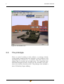
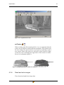
picture below [Fig. 5-1] shows the software in action combined with
detection and tracking algorithms designed to single out potential
army vehicles and calculate their shape, size, and position on the
ground. The red squares indicate a possible match.
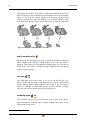
Figure 5-1: Object detection and tracking using an image sequence from
SceneServer
45
46
5.1.
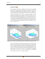
Examples of how SceneServer is used
Simulation of target approaches
SceneServer has been used to analyse how different ways of
approaching a target can affect classification. The following examples show images from two different tests ran in SceneServer. The
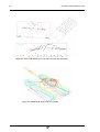
top two images show the flight paths. The one to the left is the path in
the xy-plane, while the one to the right shows how the altitude
changes through time. The eight images in the middle are from a simulation made using IR textured models in SceneServer, and correspond to what would be seen during the approach using an IR sensor.
The final eight images are colour coded depth buffer images from
SceneServer, and simulate the use of a laser radar system.
The first scenario [Fig. 5-2] is a target approach along a straight line,
the altitude decreasing linearly. In the second scenario [Fig. 5-3] the
flight path is curved (270 degrees) and the altitude increases at the
end of the course of events.
Examples of how SceneServer is used
Figure 5-2: Images from the first target approach
47
48
Examples of how SceneServer is used
Figure 5-3: Images from the second target approach
Examples of how SceneServer is used
5.2.
Recognition using laser
SceneServer has been used in the ISM project [Section 1.2.2] to create a model database. Each object is stored as a vertex list, and for
every object a number of copies with differently articulated parts can
be saved.
In the ISM project, information from laser radar, IR cameras, and
CCD* cameras are combined in order to get a better classification of
objects.
The data gathered when using a laser radar system are a number of
points in 3D space. The data is first examined from above. Information about the object’s dimensions can be extracted, and possible subparts can be defined. The object’s rotation around one axis can also
be calculated. The data is then examined from other views, and the
remaining rotations are determined [Fig. 5-4].
The object’s size, and other distinct attributes, are used to decrease
the number of possible models to match the object with.
The points are then matched with correctly rotated vertex lists from
conceivable models and a best match is computed [Fig. 5-5].
*.
Charge Coupled Device, a technique that improves resolution in cameras
49
50
Examples of how SceneServer is used
Figure 5-4: Laser radar data from a T-72 tank seen from three directions
Figure 5-5: Matching the points with a T-72 model
6. Future work
When we began our work developing SceneServer we had a set of
key features listed in the specification of this thesis [Section 1.1],
assembled by our supervisor Jörgen Ahlberg. These features together
with the topics discussed in the pre-study [Section 2.4] formed a
rather large task to take on. However, time rather than technical difficulties set the limit for us regarding the number of functions that we
managed to implement in SceneServer. This leaves a number of interesting subjects to address in the future development of this software.
When revising the items gathered in the pre-study we have found the
following points, which have not yet been implemented, to be interesting subjects for future work.
Group A
All functions implemented.
Group B
• Generate textures: This could be useful in matching algorithms, to
evaluate the probability of a correct match by applying the generated
texture to an object and calculate the degree of divergence between
images rendered with and without an object.
• Paths: It would be useful to have a function that can calculate a path,
some sort of spline function, from a set of checkpoints. Objects could
then be assigned to follow that path with a specified velocity using the
tripod function.
Group C
• Small objects: This function should override the limits of the graphic
system, that an object smaller than a pixel is discarded. By sub-sampling the object and calculate an average value that is applied to the
rendered image the system would not discard valuable information.
• Shadows: A function for generating shadows cast by objects would
improve the quality of the rendered images. This feature has not been
prioritized due to the fact that the most work has been concentrated to
the non visual spectrum (IR, laser) where shadows simply do not
appear in the same manner.
• Collision detection: A first step towards a collision detection system
has already been taken with the implementation of getIntersection
[Section 4.3.5]. A future system might use this in combination with
other techniques.
51
52
Future work
• Dynamic selection: The Kvarn model [Section 2.3.1] is a terrain
model covering a large area subdivided into a set of patches. By creating a function that can govern which sub parts to load in order to cover
the area visible in the camera the vast amount of data that is associated
with the Kvarn model can be greatly reduced, thus leaving more memory resources free on the system.
*
In addition to the functions left from the pre-study there are some
functions that we would like to expand or refine in order to increase
the functionality in SceneServer.
The Level-of-Detail function, that for the moment discards all levels
but the one with the highest detail, could be altered in some other
way where all detail levels are preserved.
More support for object manipulation in the GUI. It would for example be nice to have a function that allows the user to pick an object by
using the mouse pointer on the screen. A similar task would be to
move specific objects by dragging them on the screen.
Retrieve more data from SceneServer to MATLAB. This could mean
collecting all variables affecting an object such as position, size, and
texture information. If the objects could be placed more easily in the
GUI, as described in the paragraph above, this function would ensure
an effortless transmission of the position data to MATLAB.
Finally we would like to mention that an implementation of particle
systems in SceneServer would open the door to more advanced environmental simulations such as twirling particles under water. We are
planning to address this topic in our future work with SceneServer at
FOI.
7. Conclusion
Scene graph technology can be used in a 3D software to produce test
material for developers of computer vision algorithms, not only for
the visible light range. Using models with material properties making
them non-affected by lighting conditions, and with replaceable IR
textures, it can also be used for the IR range. With the possibility to
access depth buffers, send beams to check for intersections, and get
vertex lists transformed by the transform matrices for objects and
their parts, it can also be used in the laser area.
A couple of examples of the usage of SceneServer have been shown
in this thesis [Section 5].
During the development, SceneServer was already used in some of
the involved projects at FOI. Because of this we got good feedback,
and could make necessary changes to the application. The prioritisation that was decided after the pre-study [Section 2.4] was changed a
couple of times during the implementation in discussion with our
supervisor, since other areas became more important.
All of the items mentioned in the highest prioritized group in the prestudy [Section 2.4.1] have been implemented. These functions are
essential and had to exist if the software should be useful. Among the
items in the second group [Section 2.4.2], everything but object paths
and textures generated from the area hidden by an object are implemented.
We have focused on one of the items in the last list [Section 2.4.3].
Being able to extract vertex lists from transformed objects became
more important and was given a higher priority during the development. It also became interesting to be able to insert objects described
by matrices in MATLAB into SceneServer. Because of this we implemented a number of functions for handling vertex lists, colour lists,
and texture lists [Section 4.3.6].
53
54
8. References
[1]
The Swedish Defence Research Agency, FOI, <www.foi.se>.
[2]
OpenFlight, <http://www.multigen.com/products/standards/openflight/index.shtml>.
[3]
M. Woo, J. Neider, T. Davis, and D. Shreiner, OpenGL Programming Guide Third
Edition, Addison-Wesley, 1999.
[4]
OpenGL, <www.opengl.org>.
[5]
D. Reiners, Scene Graph Rendering, 2002,
<http://www.vrjuggler.org/pub/scenegraph-rendering.ieeevr2002.pdf>.
[6]
Open Scene Graph, <www.openscenegraph.org>.
[7]
E. Gamma, R. Helm, R. Johnson, and J. Vlissides, Design Patterns, Addison-Wesley,
1995.
[8]
MSDN, <http://msdn.microsoft.com/library/default.asp>.
[9]
D. Hearn, and M. P. Baker, Computer Graphics Second Edition, Prentice Hall,1997.
[10]
D. Eberly, Euler Angle Formulas, Magic Software, 1999,
<http://www.magic-software.com/Documentation/EulerAngles.pdf>.
[11]
T. Akenine-Möller and E. Haines, Real-Time Rendering, A K Peters Ltd, 2002.
55
56
Appendix A: User guide
During the development of SceneServer we built a homepage with
information about the software. Among other things, the homepage
included a list, which can be seen in this appendix, with descriptions
of every available MATLAB function.
MATLAB functions
Legend
[0-1] the variable could be between 0 and 1
[0|1] the variable could be either 0 or 1
TYPE object the variable 'object' can be specified using different types, i.e. int and String
[optional] this variable can be excluded
boolean 0 = false, 1 = true
General SceneServer functions
ss = sireoslib.SceneServerLib.getLib;
Create a pointer to the Java class communicating with the application.
No arguments
ss.setTimeout (int time);
Sets the timeout in seconds. If the server does not reply within the timeout a network error will
occur. The special case time=0 means that Java will wait for reply for unlimited time.
- time: time in seconds (as default, time=0)
ss.setIP (String IP_number);
Sets the IP to the computer where the SceneServer application is running
- IP_number: As default, IP = '127.0.0.1' (localhost)
Camera and viewport settings
boolean ss.setLookAt(double eye_x, double eye_y, double eye_z, double center_x,
double center_y, double center_z, double up_x, double up_y, double up_z);
Set look at specifies the camera look at
- eye: The x,y and z coordinate of the camera
- center: The x,y and z coordinate of the center point
- up: Specifies the upvector for the camera
57
boolean ss.setPerspective (double FOV_y, int width, int height, double near_plane,
double far_plane);
Set perspective projection.
- FOV_y: Field of view in degrees.
- width: Screen width in pixels
- height: Screen height in pixels
- near_plane: Distance to near cutting plane (all objects closer than this will be cut)
- far_plane: Distance to far cutting plane (all objects farther away than this will be cut)
boolean ss.setPerspective (double FOV_y, int width, int height);
Set perspective projection, without changing the current near/far plane computation values.
boolean ss.setOrtho (int screen_width, int screen_height, double viewport_width);
Set orthographic projection. Viewport height will be calculated using (screen_height/
screen_width)*viewport_width.
- screen_width: Screen width in pixels
- screen_height: Screen height in pixels
- viewport_width: Viewport width in metres
boolean ss.setLOD(int distance);
Sets the distance of highest level of detail of the objects in the scene
- distance: The distance in metres from the viewport
boolean ss.osgComputeNearFar();
OpenSceneGraph computes near/far planes using bounding boxes. This is default, but can
be changed with setPerspective
boolean ss.setLight(double pos_x, double pos_y, double pos_z, double pos_w, double
ambient_r, double ambient_g, double ambient_b, double ambient_a, double diffuse_r,
double diffuse_g, double diffuse_b, double diffuse_a, double specular_r, double
specular_g, double specular_b, double specular_a);
Set light specifies the location and colour of the light
- pos: four values, x, y, z, w. If the last value, w, is zero, the corresponding light source is a
directional one, and the (x,y,z) values describe its direction (for example 0,0,1,0). If the w
value is nonzero, the light is positional, and the (x,y,z) values specify the location of the light
(for example 0,0,10,1)
- ambient[0-1]: The red,green,blue and alpha value of the ambient light
- diffuse[0-1]: The red,green,blue and alpha value of the diffuse light
- specular[0-1]: The red,green,blue and alpha value of the specular light
boolean ss.setBackground(double red, double green, double blue, double alpha);
Sets the background colour, RGBA [0-1]
58
boolean ss.setFog(double density, double red, double green, double blue, double
alpha, int mode);
Set fog effect in the scene
- density: The density of the fog
- colour[0-1]: RGBA sets the colour of the fog
- mode[1|2]: Two exponential fog modes, GL_EXP and GL_EXP2
boolean ss.autoUpdateView(boolean update);
Toggle automatic update after every command on/off.
- update[0|1]: 0 = only update when a ss.updateView command is executed, 1 = update after
every command (default)
boolean ss.updateView();
Render the current view. Only needs to be done if ss.autoUpdateView(0) is set.
Read, edit and save objects
boolean ss.clear;
Clear current scene graph, all objects are removed
boolean ss.readScene(String filename, String name);
Read scene reads an object without specifying the coordinate transform
- filename: The file path
- [optional] name: specify the name to be set for the scene object (if no name is set, an object
name like 'Object1' will be created and printed in MATLAB)
59
boolean ss.readObject(String filename, double translation_x, double translation_y,
double translation_z, double rotation_x, double rotation_y, double rotation_z, double
scale_x, double scale_y, double scale_z, String name);
Read object specifying translation, rotation and scale.
- filename: The file path
- translation: Translate in the x,y and z world coordinates
- rotation: Rotate the object in XYZ order (Radians)
- scale: The scaling in x, y and z
- [optional] name: specify the name to be set for the object
boolean ss.readObject(String filename, double translation_x, double translation_y,
double translation_z, double rotation_x, double rotation_y, double rotation_z, String
name);
Read object with scale set to 1
- [optional] name: specify the name to be set for the object
boolean ss.readObject(String filename, double translation_x, double translation_y,
double translation_z, String name);
Read object with scale set to 1 and no rotation
- [optional] name: specify the name to be set for the object
boolean ss.editObject(TYPE object, double translation_x, double translation_y, double
translation_z, double rotation_x, double rotation_y, double rotation_z, double scale_x,
double scale_y, double scale_z);
Edit object: translation, rotation and scaling
- object: The object can be specified by an int or a String
- translation: Translate in the x,y and z world coordinates
- [optional] rotation: Rotate the object in XYZ order (Radians)
- [optional] scale: The scaling in x, y and z
boolean ss.editPart(TYPE object, String partName, double translation_x, double
translation_y, double translation_z, double rotation_x, double rotation_y, double
rotation_z, double scale_x, double scale_y, double scale_z);
Edit object part: translation, rotation and scaling.
- object: The object can be specified by an int or a String
- partName: Name of part transform (DOF Transform). Could be 'turret',
'gun' or 'missile' depending on the model. Possible partnames could by
seen by using "View Scene Graph" in the SceneServer application (see
image) or by using ss.viewSceneGraph from MATLAB.
- translation: Translate in x,y and z (origin is the origin defined for the
part)
- rotation: Rotate the object part in XYZ order (Radians)
- scale: The scaling in x, y and z
boolean ss.editPart(TYPE object, String partName, double rotation_x, double
rotation_y, double rotation_z);
Rotate object part, no translation or scaling
60
double[ ] ss.tripod(TYPE object, double translate_x, double translate_y, double
rotate_z, double scale_x, double scale_y, double scale_z, double step_x, double
step_y, double center_x, double center_y, double descend);
Assign a tripod to govern the placement of the object in the scene.
- object: The object can be specified by an int or a String
- translate: Translate object in the x and y world coordinates
- rotate: Rotate in XYZ order (Radians)
- scale: Scale object in x, y and z
- step: Sets the x-,y-distances of the tripod from its centerpoint in object coordinate system
- center: Sets the center point x-, y-coordinate of the tripod in object coordinate system
- descend: Sets how much the object should sink into the ground
- RETURNS: Rotation and z-translation as double values [rot_x, rot_y, rot_z, translation_z]
double[ ] ss.tripod(TYPE object, double translate_x, double translate_y, double
rotate_z, double step_x, double step_y, double center_x, double center_y, double
descend);
Assign tripod without scaling the object.
double[ ] ss.tripod(TYPE object, double translate_x, double translate_y, double
rotate_z, double step_x, double step_y, double descend);
Assign tripod without scaling and setting the centerpoint. The object's center point will be the
object's default center point
boolean ss.deleteObject(TYPE object);
Removes the specified object from the scene graph. deleteObject will not free memory if the
object was read from a .flt file (this is a problem with OSG). Models can be converted to .osg
by using saveObjectAsOSG.
- object: The object can be specified by an int or a String
boolean ss.deletePart(TYPE object, int ID);
Removes the specified part from the object. deletePart will not free memory if the object was
read from a .flt file (this is a problem with OSG). Models can be converted to .osg by using
saveObjectAsOSG.
- object: The object can be specified by an int or a String
- ID: The part can be specified by an int. The ID for each part is listed using
ss.viewSceneGraph from MATLAB.
boolean ss.viewSceneGraph(TYPE object);
Lists the nodes in the specified object as ID:# NAME(TYPE).
- object: The object can be specified by an int or a String
61
boolean ss.setTexture(TYPE object, String textureFile);
Sets the texture of the specified object
- object: The object can be specified by an int or a String
- textureFile: specify the path and filename to a texture file (RGB, BMP, JPG)
boolean ss.setTexture(TYPE object, String textureFile1, String textureFile2);
Sets the texture of the specified object. If the object only has one texture image, the second
specified texture file is ignored.
- object: The object can be specified by an int or a String
- textureFiles: Path and filename to the two texture files (RGB, BMP, JPG)
int ss.getObjectNumber(String name);
Retrieves the object number for the object with the specified name
- RETURNS: Object number
boolean ss.saveObjectAsOSG(TYPE object, String fileName);
Saves the specified object as a .osg model. The file should be placed in the same folder as
the texture and attribute files.
- object: The object can be specified by an int or a String
- fileName: The file path (should end with .osg)
Read and write images
byte[ ] ss.getImage();
Retrieves the image rendered in the SceneServer application.
----EXAMPLE---a=ss.getImage;
a=double(a)./255;
a = a + (a<0)*1;
height=ss.getHeight;
width=ss.getWidth;
img = zeros(height,width,3);
img(:,:,1) = reshape(a(1:3:length(a)),width,height)';
img(:,:,2) = reshape(a(2:3:length(a)),width,height)';
img(:,:,3) = reshape(a(3:3:length(a)),width,height)';
figure;
imshow(img);
62
double[ ] ss.getDoubleImage();
Retrieves the image rendered in the SceneServer application as a double array with values
between 0 and 1.
----EXAMPLE---a=ss.getDoubleImage;
height=ss.getHeight;
width=ss.getWidth;
img = zeros(height,width,3);
img(:,:,1) = reshape(a(1:3:length(a)),width,height)';
img(:,:,2) = reshape(a(2:3:length(a)),width,height)';
img(:,:,3) = reshape(a(3:3:length(a)),width,height)';
figure;
imshow(img);
boolean ss.writeImageFile(String file);
Writes the image rendered in the SceneServer application to the specified file (.BMP)
Image depth and intersection
double[ ][ ] ss.getDepthBuffer();
Retrieves the depth buffer as a matrix with the dimensions of the SceneServer application
window
Values are scaled to match distance to viewport.
double[ ] ss.getIntersection(double start_x, double start_y, double start_z, double
stop_x, double stop_y, double stop_z);
Sends a line between the specified points and retrieves the x, y, z coordinates of the first
intersection
NOTE: If no intersection is found the function returns the stop coordinates
- RETURNS: intersection point [x,y,z]
double[ ] ss.getObjectIntersection(TYPE object, double start_x, double start_y, double
start_z, double stop_x, double stop_y, double stop_z);
Sends a line between the specified points and retrieves the x, y, z coordinates of the first
intersection with the specified object
NOTE: If no intersection is found the function returns the stop coordinates
- object: The object can be specified by an int or a String
- RETURNS: intersection point [x,y,z]
63
Scene Graph manipulation from MATLAB
boolean ss.createObject(String name, double translate_x, double translate_y, double
translate_z, double rotate_x, double rotate_y, double rotate_z, double scale_x, double
scale_y, double scale_z);
Create an object with an empty Geode called name_geode, and a transform called
name_transform. The transform can be edited by using ss.editPart
- name: This sets the name of the object
- translation: Translate in the x,y and z world coordinates
- rotation: Rotate in XYZ order (Radians)
- scale: The scaling in x, y and z
boolean ss.addChild(TYPE object, String name, String parent, String type);
Adds a child of type Geode(for storing geometries) or transform.
- object: The object can be specified by an int or a String
- name: This sets the name of the new child
- parent: Specifies the name of the parent
- type: Two types supported ('geode' or 'transform')
boolean ss.setVertexList(TYPE object, String geodeName, double[ ][ ] vertexList, int
vertexListSize, int[ ][ ] faceList, int faceListSize, int mode, int wireframe);
Set the vertex list in the specified Geode
- object: The object can be specified by an int or a String
- geodeName: The name of the Geode to set the vertex list in
- vertexList: A 3*vertexListSize matrix containing the x,y and z coordinate to every vertex
- vertexListSize: The number of vertices in the vertex list.
- faceList: A 3*faceListSize matrix if triangles, 4*faceListSize matrix if quads, containing the
vertices defining each face. If an empty face list with faceListSize = 0 is sent, SceneServer
will create a faceList [0 1 2;3 4 5...]
- faceListSize: The number of faces in the face list
- mode[4|7]: Sets the geometry mode, currently triangles = mode 4, quads = mode 7
- wireframe[0|1]: Sets the vertex list as wireframe if 1
double[ ][ ] ss.getVertexList(TYPE object, int mode);
Get an object's vertex list in triangles. The vertex list is computed from the current articulation
of the object (done by using editPart).
- object: The object can be specified by an int or a String
[optional] mode[0|1]: 0 = part transforms, no object transforms (default), 1 = part and object
transforms
----EXAMPLE---vertexList = ss.getVertexList(myObject);
faceList = reshape([1:(size(vertexList,1))],3,(size(vertexList,1))/3)';
trimesh(faceList,vertexList(:,1),vertexList(:,2),vertexList(:,3));axis equal;
64
boolean ss.setVertexColorList(TYPE object, String geodeName, double[ ][ ]
vertexColorList, int vertexColorListSize);
Set the vertex colour list in the specified Geode
- object: The object can be specified by an int or a String
- geodeName: The name of the Geode to set the vertex colour list in
- vertexColorList: A 4*vertexColorListSize matrix containing the red,green, blue and alpha
values to every face
- vertexColorListSize: The number of colours in the vertex colour list.
boolean ss.setVertexTextureList(TYPE object, String geodeName, double[ ][ ]
vertexTextureList, int vertexTextureListSize, String textureFile);
Set the vertex texture list in the specified Geode
- object: The object can be specified by an int or a String
- geodeName: The name of the Geode to set the vertex texture list in
- vertexTextureList: A 2*vertexTextureListSize matrix containing the coordinates for each face
in the texture file
- vertexTextureListSize: The number of texture coordinates in the vertex texture list.
- textureFile: specify the path and filename to a texture file (RGB, BMP, JPG)
65
66