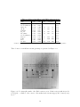
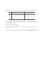
1
Subaru Telescope
Infrared Camera
and Spectrograph (IRCS)
User Manual
Ver. 1.0.1
K. G. Helminiak, T.-S. Pyo, J.-H. Kim, M. Morris
National Astronomical Observatory of Japan
May 2015
Change record:
• 1.0.0 – March ’15: first version prepared, mainly for proposal preparation [KGH]
• 1.0.1 – June ’15: Added: OPE files, Appendix and info on output data. Figures 1.1
and 3.1 changed. Grism slit lengths added. Authors added. Other major and minor
comments from TSP, JHK and MM addressed. Corrected language (JB) and some typos.
[KGH]
2
Contents
1 Introduction
1.1 Scope . . . . . . . . . . . . . . . . . . . . . . . . . . . . . . . . . . . . . . . . .
1.2 Additional Information . . . . . . . . . . . . . . . . . . . . . . . . . . . . . . . .
1.3 Abbreviations . . . . . . . . . . . . . . . . . . . . . . . . . . . . . . . . . . . . .
6
6
6
7
2 General information
2.1 Overall Description . . . . . . . . . . . . . . . . . . . . . . . . . . . . . . . . . .
2.2 AO188 adaptive optics system . . . . . . . . . . . . . . . . . . . . . . . . . . . .
2.3 Output files and data access . . . . . . . . . . . . . . . . . . . . . . . . . . . . .
8
8
8
9
3 Observing modes
3.1 Imaging . . . . . . . . . . . . . . . . . .
3.1.1 Detector . . . . . . . . . . . . . .
3.1.2 Filters . . . . . . . . . . . . . . .
3.1.3 Coronagraphy . . . . . . . . . . .
3.1.4 Image anomalies . . . . . . . . .
3.1.5 Imaging calibrations . . . . . . .
3.1.6 Imaging data reduction . . . . .
3.2 Grism spectroscopy . . . . . . . . . . . .
3.2.1 Reflective slits . . . . . . . . . .
3.2.2 Grisms and order sorting filters .
3.2.3 Sensitivity corrections . . . . . .
3.2.4 Grism spectroscopy calibrations .
3.2.5 Grism data reduction . . . . . .
3.3 Echelle spectroscopy . . . . . . . . . . .
3.3.1 Detector . . . . . . . . . . . . . .
3.3.2 Echelle configurations . . . . . .
3.3.3 Sensitivity corrections . . . . . .
3.3.4 Single-order filters . . . . . . . .
3.3.5 Ammonia (NH3 ) cell . . . . . . .
3.3.6 Echelle calibrations . . . . . . . .
3.3.7 Echelle data reduction . . . . . .
3.4 Polarimetry (shared risk) . . . . . . . .
3
.
.
.
.
.
.
.
.
.
.
.
.
.
.
.
.
.
.
.
.
.
.
.
.
.
.
.
.
.
.
.
.
.
.
.
.
.
.
.
.
.
.
.
.
.
.
.
.
.
.
.
.
.
.
.
.
.
.
.
.
.
.
.
.
.
.
.
.
.
.
.
.
.
.
.
.
.
.
.
.
.
.
.
.
.
.
.
.
.
.
.
.
.
.
.
.
.
.
.
.
.
.
.
.
.
.
.
.
.
.
.
.
.
.
.
.
.
.
.
.
.
.
.
.
.
.
.
.
.
.
.
.
.
.
.
.
.
.
.
.
.
.
.
.
.
.
.
.
.
.
.
.
.
.
.
.
.
.
.
.
.
.
.
.
.
.
.
.
.
.
.
.
.
.
.
.
.
.
.
.
.
.
.
.
.
.
.
.
.
.
.
.
.
.
.
.
.
.
.
.
.
.
.
.
.
.
.
.
.
.
.
.
.
.
.
.
.
.
.
.
.
.
.
.
.
.
.
.
.
.
.
.
.
.
.
.
.
.
.
.
.
.
.
.
.
.
.
.
.
.
.
.
.
.
.
.
.
.
.
.
.
.
.
.
.
.
.
.
.
.
.
.
.
.
.
.
.
.
.
.
.
.
.
.
.
.
.
.
.
.
.
.
.
.
.
.
.
.
.
.
.
.
.
.
.
.
.
.
.
.
.
.
.
.
.
.
.
.
.
.
.
.
.
.
.
.
.
.
.
.
.
.
.
.
.
.
.
.
.
.
.
.
.
.
.
.
.
.
.
.
.
.
.
.
.
.
.
.
.
.
.
.
.
.
.
.
.
.
.
.
.
.
.
.
.
.
.
.
.
.
.
.
.
.
.
.
.
.
.
.
.
.
.
.
.
.
.
.
.
.
.
.
.
.
.
.
.
.
.
.
.
.
.
.
.
.
.
.
.
.
.
.
.
.
.
.
.
.
.
.
.
.
.
.
.
.
.
.
.
.
.
.
.
.
.
.
.
.
.
.
.
.
.
.
.
.
.
.
.
.
.
.
.
.
.
.
.
.
.
.
.
.
.
.
.
.
.
.
.
.
.
.
.
.
10
10
11
13
13
15
15
15
16
16
16
16
18
19
20
20
21
23
23
24
24
24
25
3.4.1
3.4.2
3.4.3
Polarization efficiency . . . . . . . . . . . . . . . . . . . . . . . . . . . .
Instrumental polarization . . . . . . . . . . . . . . . . . . . . . . . . . .
Unpolarized and standard stars . . . . . . . . . . . . . . . . . . . . . . .
4 Preparing and executing observations
4.1 Exposure times and their calculators . . . . . . . . . .
4.1.1 Imaging . . . . . . . . . . . . . . . . . . . . . .
4.1.2 Grism spectroscopy . . . . . . . . . . . . . . .
4.1.3 Echelle spectroscopy . . . . . . . . . . . . . . .
4.2 Coadds and data cubes . . . . . . . . . . . . . . . . .
4.3 Dithering, nodding, object-sky-object and slit scanning
4.3.1 Dithering in the imaging mode . . . . . . . . .
4.3.2 ABBA slit nodding . . . . . . . . . . . . . . . .
4.3.3 Object-Sky-Object . . . . . . . . . . . . . . . .
4.3.4 Slit scanning . . . . . . . . . . . . . . . . . . .
4.4 Overheads and total observing time calculators . . . .
4.4.1 Common overheads . . . . . . . . . . . . . . . .
4.4.2 OTCs . . . . . . . . . . . . . . . . . . . . . . .
4.4.3 Polarimetry – a special case . . . . . . . . . . .
4.5 Spectral format calculators . . . . . . . . . . . . . . .
4.6 OPE file . . . . . . . . . . . . . . . . . . . . . . . . . .
4.6.1 List of targets . . . . . . . . . . . . . . . . . . .
4.6.2 Observing procedure . . . . . . . . . . . . . . .
26
26
26
.
.
.
.
.
.
.
.
.
.
.
.
.
.
.
.
.
.
28
28
28
30
30
31
32
32
32
33
33
33
33
33
35
35
36
36
37
5 Appendix
5.1 Fits header . . . . . . . . . . . . . . . . . . . . . . . . . . . . . . . . . . . . . .
5.2 OH emission lines . . . . . . . . . . . . . . . . . . . . . . . . . . . . . . . . . . .
5.3 Ar lines atlas for grism spectroscopy . . . . . . . . . . . . . . . . . . . . . . . .
42
42
50
58
4
.
.
.
.
.
.
.
.
.
.
.
.
.
.
.
.
.
.
.
.
.
.
.
.
.
.
.
.
.
.
.
.
.
.
.
.
.
.
.
.
.
.
.
.
.
.
.
.
.
.
.
.
.
.
.
.
.
.
.
.
.
.
.
.
.
.
.
.
.
.
.
.
.
.
.
.
.
.
.
.
.
.
.
.
.
.
.
.
.
.
.
.
.
.
.
.
.
.
.
.
.
.
.
.
.
.
.
.
.
.
.
.
.
.
.
.
.
.
.
.
.
.
.
.
.
.
.
.
.
.
.
.
.
.
.
.
.
.
.
.
.
.
.
.
.
.
.
.
.
.
.
.
.
.
.
.
.
.
.
.
.
.
.
.
.
.
.
.
.
.
.
.
.
.
.
.
.
.
.
.
.
.
.
.
.
.
.
.
.
.
.
.
.
.
.
.
.
.
.
.
.
.
.
.
.
.
.
.
.
.
.
.
.
.
.
.
.
.
.
.
.
.
.
.
.
.
.
.
.
.
.
.
.
.
Preface
This manual was prepared by a user for a user. In its current version, this document is
intended to help in preparation of the proposal for the IRCS instrument, and then to perform
the observations. It may not immediatelly contain all required information, so you may find
blank spaces and “...” signs, but we work to include all that is necessary.
We appreciate your feedback. If you think some important information are missing, let us
know, and we’ll try to include it in the future.
KGH
5
Chapter 1
Introduction
1.1
Scope
The scope of this manual is to cover all aspects of the Subaru Telescope instrument IRCS
necessary to prepare and conduct successful observations, and collect them in a single, up-todate, handy document. It is not however intended to explain the operations itself in details,
only what is required from the user’s point of view. This manuscript includes:
• Overall description of the IRCS and its components
• Characteristics of the observing modes
• Tools and templates useful for preparing the observations
1.2
Additional Information
We tried to gather as much important information as possible, but we might still be missing
some. If you can’t find what you need, please refer to the instrument website:
http://www.naoj.org/Observing/Instruments/IRCS/index.html
and the links and references therein. Some information may be slightly different, we tried to
put the most recent ones in here.
Two papers describing the IRCS are available:
• Tokunaga et al.: http://www.naoj.org/Observing/Instruments/IRCS/spie1998.pdf
(900 kB)
• Kobayashi et al.: http://www.naoj.org/Observing/Instruments/IRCS/spie2000.ps.gz
(2 MB)
Questions regarding IRCS should be directed to Ji Hoon Kim (jhkim [at] naoj.org) or
Tae-Soo Pyo (pyo [at] naoj.org).
6
Figure 1.1: Location of the IRCS (blue box) at the Nasmyth IR (NsIR) platform. The black,
semi-transparent box is AO188. The blue wall to the left separates the NsIR platform from
the telescope.
1.3
Abbreviations
AO – adaptive optics
BLIP – background-limited performance
FOV – field of view
IMR – image rotator
IR – infrared
IRCS – Infrared Camera and Spectrograph
LGS – laser guide star
NDR – non-destructive readout
NGS – natural guide star
OSF – order-sorting filter
TT – tip-tilt
7
Chapter 2
General information
2.1
Overall Description
The Infrared Camera and Spectrograph (IRCS) is a multi-purpose instrument, designed to
work in the near infra-red regime from 0.9-5.6 µm, covering photometric bands from Iz to M 0 .
It can be installed in the IR Nasmyth focus of the Subaru Telescope. It consists of two modules
– the imaging camera and the echelle spectrograph – both equipped with 1024×1024×27µm
ALADDIN III InSb detectors. The instrument works with the AO188 adaptive optics system,
both in natural and laser guide star modes, and is capable of providing diffraction-limited
images. Spectroscopy can be performed either with the echelle spectrograph or with the
camera using grisms. Switching between observing modes is relatively fast and only requires
moving the slit and/or filter wheels to a different position. The observing modes are described
in more details in the following Chapter.
The choice of the observing mode is done by selecting an appropriate element on the slit
wheel, which is installed on the light path before any filter wheel. Light is reflected to the
camera section by a plain mirror or coronagraph mask for imaging, reflective slits for grism
spectroscopy, or polarimetric masks for both imaging and spectropolarimetry. The light is
transmitted to the echelle section through one of the slits cut in reflecting mirrors. In such
configuration the camera section serves as the slit viewer.
2.2
AO188 adaptive optics system
The IRCS is currently fed by the AO188 adaptive optics system. Even if the correction is not
applied, the light goes first through the AO optics1 . The detailed description is provided at
this website:
http://www.naoj.org/Observing/Instruments/AO/index.html
however, we present some information here as they are required to prepare the IRCS proposal
and observations.
1
It’s also possible to remove AO188 so that light goes directly to IRCS. This is, however, rarely done and
must be done by the daycrew
8
AO188 is equipped with a 188-element wavefront curvature sensor with photon counting
APD modules and a 188 element bimorph mirror. AO188 is installed at the IR Nasmyth
platform of Subaru telescope, and can be used in either natural guide star (NGS) or laser
guide star (LGS) mode. Diffraction-limited spatial resolution can be achieved at KLM bands
with a sufficiently bright guide star at good observing conditions. At shorter wavelength (zJH
band), high spatial resolution comparable to or even higher than the K-band diffraction-limit
resolution can be achieved, however the Strehl ratio is lower. The maximum Strehl ratio so
far achieved at K-band is 0.55 at a 0.5” seeing condition.
For the NGS mode operation, a natural guide star is required. The guide star should be
brighter than R = 16.5 mag, located within 30” of the science target. Please note, that the
image quality degrades rapidly with the distance. The science target may be used as NGS.
For the LGS mode operations, a natural tip-tilt guide star (TTGS) is still required to
correct for the tip-tilt motion that cannot be sensed by the LGS. Point sources, brighter
than R = 18 mag, located less than 60” from the target are recommended, however in some
circumstances extended or non-sidereal objects are allowed. The science target itself can be
used as the TTGS.
For both LGS and NGS modes we recommend you to observe at elevations > 45◦ .
The distortion maps for IRCS+AO188 combination, together with the IRAF script for
correction, are available from this URL:
http://www.naoj.org/Observing/Instruments/IRCS/camera/IRCS+AO188 distortion/
2.3
Output files and data access
The raw output files are 1024×1024 pix (or sub-array size) fits files, which name starts with
IRCA. One file is made at one telescope position, which means that for an observation in 5point dither mode (see Fig. 4.1) you will get 5 output files, no matter how many coaadds are
defined. See Section 5.1 in the Appendix for a sample IRCS fits file header.
The data can be obtained at the summit, just after the observations. You can also ask
for data delivery. Please fill in the Observation Data Request Form and submit it to the
Operation Center. If you have already received your data at the summit, please inform on the
form as well. The copy of your observation data will be available as following formats, and
please inform your preference on the request form:
• Sending either DAT or DLT media format (visiting observes only). Please choose a
preferable media format and write your address on the request form. We will send the
item within a week.
• Obtaining data by yourself through Subaru Telescope Archive System (STARS, at Subaru Telescope) or MASTARS (at Mitaka Office).
Also, the PI of the proposal will obtain a notification email with instructions about how to
access to the data at STARS/MASTARS.
The IRCS data are subject to a common Subaru priority and archiving policy. All raw
scientific data will become publicly available at the SMOKA system2 after 18 months.
2
http://smoka.nao.ac.jp/
9
Chapter 3
Observing modes
3.1
Imaging
The IRCS imaging camera offers two default pixel scales: 20 and 52 mas/pix, producing fields
of view of 21” and 54”, respectively. A third mode of 12 mas/pix scale is also available upon
request, it is, however, not commonly used, as it requires special preparations and science
targets brighter than in the case of the other two, on which we focus in this document.
Figure 3.1: Layout of the fore-optics and the camera section of the IRCS.
10
Figure 3.2: Example of a raw IRCS+AO188 image from the camera section. A group of bad
pixels near the center, and a single star right to it can be seen.
The optical layout of the camera section, together with the fore-optics, is presented in
Figure 3.1. The Figure 3.2 shows an example of a raw IRCS image in the 20 mas/pix scale.
The default orientation is North is left, and East to the bottom, with the position angle (PA)
set to 0◦ . With PA=90◦ N is up and E to the left.
3.1.1
Detector
The imaging section camera is equipped in 1024×1024×27µm ALADDIN III InSb detector.
Its basic characteristics are summarized in Table 3.11 .
In common with all ALADDIN arrays, there is some latency. For the current IRCS camera
array, latent images are seen at the level of ∼0.1% if the wells have been more than half-filled.
For this reason, it is recommended to keep your counts well below the saturation level. The
detector also has a number of bad pixels, concentrated mainly at the edges, but also close to
the center in the first quadrant (Fig. 3.2). They can be corrected using the bad pixel mask:
http://www.naoj.org/Observing/Instruments/IRCS/camera/cam badpix.pl
or .../cam badpix.coo
1
If you need the old parameters (before July 2005, when IRCS was mounted on Cassegrain focus) please see
http://www.naoj.org/Observing/Instruments/IRCS/parameters.html.050810
11
Table 3.1: Basic parameters of the IRCS imaging camera
Mode:
20 mas
52 mas
a
Pixel scale
20.57±0.04 mas 52.77±0.04 mas
FOVa
21.06 arcsec2
54.04 arcsec2
−
Gain
5.6 e /ADU
Dark current
0.1 e− /s
b
Readout noise
43 e− rms
123,000 e−
Saturation level
c
Readout rate
0.41 s (standard); 0.12 s (fast)
b
The 12 mas mode has the pixel scale of 11.94±0.01 mas
and field of view 12.22 arcsec2 .
a with AO, to convert for case without AO, divide these values by 1.007
(N/A for the 12 mas mode);
per NDR, readout noise per frame = (readout noise per NDR)/sqrt(NDR);
c for the full 1K × 1K array size.
Figure 3.3: Non-linearity of the IRCS imaging detector.
The detector shows a significant level of non-linearity at high ADU (Fig. 3.3). To achieve
linearity down to 1% we recommend a maximum signal value <4000 ADU (22,400 e− ) per
exposure. For L0 and M 0 bands, the signal level of 7000 ADU (39,200 e− ) can be allowed with
less than 3% non-linearity because of very high background level.
Keep in mind that you do not have to read out the whole 1024×1024 chip, but reading in
sub-arrays is possible, and even mandatory in some modes or filters (like the L0 filter). This,
of course, results in shorter read-out times and lower overheads. It is not possible to read any
part of the chip, only squared boxes in the center. The allowed sizes (side of square, in pix)
are: 64, 128, 256, 384, 512, 640, 768, and 896.
12
Table 3.2: Broad-band filters of the IRCS camera section
Sensitivity
mag for
[mag/as2 ]
1 e− /s
w/ AO
w/o AO
w/ AO
w/o AO
w/ AO
w/o AO
20&52 mas
20&52 mas
20&52 mas
20 mas
52 mas
20&52 mas
20&52 mas
Y
1.02
0.103
TBD
TBD
—
TBD
TBD
25.8
TBD
J
1.25
0.16
23.5
23.6
—
19.6
20.6
26.1
26.3
H
1.63
0.30
22.7
22.8
—
18.6
19.6
26.3
26.5
2.12
0.35
—
22.6
—
18.4
19.4
—
25.8
K0
K
2.20
0.34
22.2
22.3
—
18.2
19.2
25.5
25.7
L0a
3.77
0.70
—
17.1
—
13.3
14.3
24.7
24.7
4.68
0.24
—
14.6
—
10.8
—
22.5
22.6
M 0b
a L0 observation with the 52 mas pixel scale is limited to a maximum 512×512 (27”×27”) subarray with AO and
896×896 (47”×47”) subarray without AO.
b M 0 observation is limited to 20 mas pixel scale mode.
Filter
name
Center
[µm]
Width
[µm]
[mag]
Imaging in L0 and M 0 bands is very sensitive to weather and airmass, hence there are
limitations for the field of view. In the L0 band the largest allowed FOV is ∼20”×20”, so
the largest sub-array is 512×512 pix in the 52 mas scale. In the M 0 band the FOV should be
adjusted to the conditions, and the 5122 in 52 mas or full-size in 20 mas can not be guaranteed.
Please note that the fast (thermal) readout mode is suggested for L0 M 0 , but is also accepted
for NIR bands (for bright targets for example). However, frequent changes of readout mode
will result in detector problems and unnecessary delays.
3.1.2
Filters
Three filter wheels offer a wide selection of broad and narrow-band astrophysical, as well as
ND1% filters. Tables 3.2 and 3.3 summarize the characteristics of broad and narrow-band
astrophysical filters, respectively.
All sensitivities are for 5σ detections in 1 hour of on-source integration with the infrared
secondary mirror. They assume background-limited performance (see Section the guide to
exposure times). Point source sensitivities assume 0.5” seeing and a 1.0” diameter extraction
aperture, which means they do not assume AO correction. With a full correction, they would
improve by 1-2 mag. Extended source sensitivities are given per pixel (the first column is for
the 20 mas pixel scale, the second for the 52 mas pixel scale). Binning over N pixels will
improve the sensitivity by 1.25 log(N ) mag.
Observers should be aware that variations in the strength of the OH air glow can cause
changes of up to 1 mag in the sky background, with significant changes in sensitivity of the
broad-band filters.
The transmission curves of almost every filter are available as plots or ASCII lists (kindly
provided by Alan Tokunaga of the IRTF) from the following URL:
http://www.naoj.org/Observing/Instruments/IRCS/camera/filters.
3.1.3
Coronagraphy
Simple coronagraphy is possible in the imaging mode with both pixel scales. The light of a
star can be blocked by one of the masks of the following diameters: 0.15, 0.6, and 0.8 arcsec.
13
Table 3.3: Narrow-band filters of the IRCS camera section
Filter
Center Width
name
[µm]
[µm]
CH4 short
1.570
0.100
Hcont (NB1550)
1.549
0.018
1.690
0.100
CH4 long
[Fe II]
1.644
0.026
2.091
0.035
NB2090
H2 1-0
2.122
0.032
2.166
0.032
Br gamma
Kcont (NB2315)
2.314
0.030
3.050
0.152
H2 O ice
PAH
3.295
0.050
H3+
3.413
0.022
Br alpha
4.052
0.060
Scanned at cold and tilted by 5◦ in IRCS, except
Sensitivity
µJy for
[µJy]
[µJy/as2 ]
1 e− /s
1.7
60
23
0.06
—
—
—
0.25
1.7
60
23
0.06
3.3
120
47
0.40
—
—
—
0.33
3.0
110
44
0.40
3.0
110
44
0.40
—
—
—
0.63
41
2193 832
0.45
55
2900 1100
0.60
—
—
—
—
140
7500 3000
0.60
Br gamma, scanned at room temperature.
Their location on an full-size 20 mas/pix image is presented in Figure 3.4.
Figure 3.4: Coronagraphic masks of the IRCS camera section. Numbers in parenthesis are the
(X, Y )[pix] coordinates of the centers of the masks in the 20 mas (upper) and 52 mas (lower)
mode.
14
Figure 3.5: Two “ghosts” that appear when a bright source is observed through an ND filter.
3.1.4
Image anomalies
Apart from the latency and bad pixels, there are no known image anomalies common to all
the camera section settings. There is one however that occurs when using the neutral density
ND1% filter in the first filter wheel – two “ghosts” appear when a bright source is observed.
Their location is shown in Figure 3.5.
Before 2006, when the instrument was installed in the Cassegrain focus, there were two
more “ghosts” visible, produced by the beam splitter and compensator. After moving to the
Nasmyth focus, these two elements are not in use any more, and the problem does not exist.
3.1.5
Imaging calibrations
Calibrations for the imaging observations include flat field images. For the 52 mas scale dome
flats are taken by observations of a uniformly-illuminated screen installed inside the dome. For
the 20 mas an internal calibration source is inserted. In case of L0 M 0 imaging, sky flats are
taken, regardless of the pixel scale. Exposuress are done at the beginning or end of the night,
separately for each setting. A short series of lamp “ON” and “OFF” frames are taken, single
images combined, and the resulting median “ON” and “OFF” images subtracted to get the
final one.
Dark current frames are not in the calibration plan. It is possible to make bias frames, but
they are not in the standard routine.
3.1.6
Imaging data reduction
A document presenting a typical procedure to reduce and analyze the IRCS imaging data has
been prepared:
http://www.naoj.org/Observing/DataReduction/Cookbooks/IRCSimg 2010jan05.pdf
15
3.2
Grism spectroscopy
The low resolution (R = 100 − 2000) spectroscopy is performed in the camera section of the
IRCS. Three elements need to be set: reflective slit (on the slit wheel), an order-sorting filter,
and a grism (both on filter wheels). The final spectral resolution and wavelength coverage are
dependent on each of the three elements, and the pixel scale selected.
3.2.1
Reflective slits
There are two reflective slits available in the slit wheel. They are the main factor that determines the output spectral resolution. The Reflective 3W (R3W) is composed of 3 elements of
different thickness (fixed in mm), that mimic three different slit widths: 0.9”, 0.45” and 0.6”,
but only the 0.45” is available in the 20 mas mode. The Reflective 4 slit (R4) has four such
elements: 0.3”, 0.15”, 0.1”, and 0.23”, the last three being available in the 20 mas mode. As
it offers narrow widths, it should be exclusively used with the AO188, otherwise the loss of
the flux will be significant.
The selection between the elements is done under the imaging mode, by placing the target
in a corresponding acquisition point (certain X and Y values in pixels), and then the R3W
or R4 is introduced in the light path. Nodding along the slit is frequently performed in IR
observations, but note that some parts of slits are of worse quality or fall on bad pixel. See
Figure 3.6 for details. The maximum allowed length is 20 arcsec (10 for 0.1 and 0.15”), but
the lengths of the most useful parts are given in Tables 3.4 and 3.5. Remember, that the
grism mode does not have slit viewer. The accuracy of slit position depends on the telescope
tracking and the auto-guider performance.
3.2.2
Grisms and order sorting filters
A single grism can be used to provide spectra in various bands (like JHK), so the wavelength
range (band) is determined by selecting a combination of a grism with an order sorting filter
(OSF). The IRCS currently has one grism that works in the 20 mas mode but two different
spectral orders cover either the IzJ or JHK bands, and OSFs are used to set the band. Four
grisms work in the 52 mas mode, and produce spectra of higher resolution.
Tables 3.4 and 3.5 summarize the wavelength range, sensitivities and spectral resolutions
for grisms (+OSF’s) for the 20 and 52 mas modes, respectively.
3.2.3
Sensitivity corrections
All sensitivities in Tables 3.4 and 3.5 are limits for 5σ detections per pixel in 1 hour of onsource integration (usually assumed to comprise six 600 second integrations), using the 0.15”
slit. Because the spectrum is properly sampled with this slit, spectra taken with wider slits
can be binned in the dispersion direction to increase sensitivity by 1.25 log(N ) mag, where N
is the number of pixels being binned (equal to 2, 4, or 6 for the wider slits).
Further improvement in sensitivity for point sources can be done by extracting the spectrum
along several spatial pixels. Apertures between 1 and 2 times the seeing FWHM are optimum.
Corrections from Tab. 3.6 be added to the numbers in the above tables to determine the point
16
Figure 3.6: Reflective slits of the IRCS. Frop to bottom: R3W at 52 mas, R4 at 52 mas, R3W
at 20 mas, R4 at 20 mas. Some (X, Y )[pix] coordinates are noted. Note the defects on 0.9”
(R3W), 0.15” and 0.3” (R4) slits. Also note the bad pixels in the center of the image. Boxes
mark parts of slits suggested for placing an object.
17
Table 3.4: Parameters for grism spectroscopy with the 20 mas mode
Coverage
Band
[µm]
Iz
0.92-1.01
zJ
1.03-1.18
J
1.19-1.38
H
1.47-1.80
K
1.92-2.40
Approx. slit length [”]
R = λ/∆λ (vs. slit)
0.10” 0.15” 0.225” 0.45”
813
542
361
181
745
497
331
166
677
452
301
151
501
334
223
111
393
262
175
87
7.0
6.5
6.5
18.0
Sensitivity
[mag/as2 ]
16.4
16.4
16.4
15.3
14.9
Table 3.5: Parameters for grism spectroscopy with the 52 mas mode
Coverage
Band
[µm]
Iz
0.92-1.01
zJ
1.03-1.18
J
1.18-1.38
H
1.49-1.83
K
1.93-2.48
L
2.84-4.16
zJH
0.95-1.50
HK
1.40-2.50
Approx. slit length [”]
0.10”
1940
1706
1432
1146
869
331
705
442
7.0
0.15”
1249
1137
955
764
579
220
470
294
7.0
R = λ/∆λ (vs.
0.225” 0.30”
862
647
758
569
637
477
509
382
386
290
147
110
313
235
196
147
20
14
slit)
0.45”
431
379
318
255
193
73
157
98
18
0.60”
323
284
239
191
145
55
118
74
15
0.90”
216
190
159
127
97
37
78
49
15
Sensitivity
[mag/as2 ]
17.3
17.3
17.0
16.1
15.6
10.8
J=17.5, H=16.6
H=16.7, K=16.0
source sensitivity in the relevant seeing conditions. Note that the first two rows represent
image quality only attainable with AO. Please ensure you use the correct table for your choice
of grism.
Increasing the slit width will improve the sensitivity of an extended source, if its surface
brightness remains constant. Corrections to be applied to the numbers from Tables 3.4 and
3.5, are the following: +0.97 mag for 0.90” slit, +0.75 for 0.60”, +0.38 for 0.30”, and 0.0 for
0.15”. Again, sensitivity can be improved by binning in the spatial direction: 1.25 log(N ) mag,
for binning over N pixels. If the source is too extended to be nodded along the 20”-long slit,
remember to double your integration time to allow for observations of blank sky.
3.2.4
Grism spectroscopy calibrations
Calibrations for the grism spectroscopy include flat-field and Ar lamp images. As for the
imaging, flats are taken using a continuum source (halogen lamp) exposures at the beginning
or end of the night, separately for each setting. A short series of lamp “ON” and “OFF”
frames are taken, single images combined, and the resulting median “ON” and “OFF” images
subtracted to get the final one.
As for the imaging, dark current and bias frames are not in the standard routine.
The wavelength calibration is initially based on spectra of an Ar lamp, taken at the beginning or end of the night, separately for each setting. A short series of lamp “ON” and “OFF”
frames are taken, single images combined, and the resulting median “ON” and “OFF” images
18
Table 3.6: Corrections in sensitivity for a point
pixel scale
Corrections for 20 mas
Seeing 0.10” 0.15” 0.30” 0.60”
0.06” +4.8 +5.0 +5.1 +4.9
0.2”
+3.5 +3.9 +4.3 +4.3
0.5”
+2.0 +2.5 +3.2 +3.6
0.7”
+1.5 +2.0 +2.7 +3.2
1.0”
+1.0 +1.5 +2.2 +2.7
source as a function of seeing, slit width, and
0.90”
+4.7
+4.1
+3.6
+3.3
+2.9
Corrections
0.15” 0.30”
+4.2 +4.2
+3.2 +3.4
+1.8 +2.4
+1.5 +2.1
+0.9 +1.6
for 52 mas
0.60” 0.90”
+4.1 +3.9
+3.6 +3.4
+2.9 +2.9
+2.5 +2.6
+2.0 +2.1
subtracted to get the final one. The wavelength solution may also be based on the atmospheric
bands in the L band, but not on the OH emission lines, due to the low spectral resolution. See
Section 5.3 in the Appendix.
3.2.5
Grism data reduction
A document presenting a typical procedure to reduce and analyze the IRCS grism spectra has
been prepared:
http://www.naoj.org/Observing/DataReduction/Cookbooks/IRCSsp cookbook 2010jan05.pdf
19
Figure 3.7: Layout of the echelle spectrograph section of the IRCS.
3.3
Echelle spectroscopy
The second major section of the IRCS is the echelle spectrograph. The light passes to it
through one of the slits in the slit wheel, that are cut in flat mirrors, and what is reflected,
goes to the camera section, which serves as a slit viewer in this configuration. The layout is
presented in Figure 3.7. The pixel scale is 55 mas along the pixel scale and slit widths of 0.14”,
0.27” and 0.56” are available. The echelle offers spectral resolution R ∼ 20, 000 (0.14” slit)
and observations from Iz to M bands (0.9-5.34 µm). Unlike grism spectroscopy, observations
at JHK with the echelle are detector-limited between OH lines. Sky subtraction is therefore
not an issue, and long exposures can be made with the target at a single slit position.
3.3.1
Detector
The ALADDIN III detector of the echelle section is the same 1024×1024×27µm InSb array as
in the camera section. It, however, operates in a slightly different pixel scale, lower gain, and
the read out parameters are a bit different. The basic information is summarized in Table 3.7.
This detector also suffers from non-linearity. Signal levels below 6000 ADU (22,800 e− )
are recommended to achieve linearity better than 1%. For this detector a bad pixel map
is also available. There are more bad pixels than for the imaging array, and they are more
concentrated, thus it is highly recommended to use this map for the data reduction.
http://www.naoj.org/Observing/Instruments/IRCS/echelle/spg badpix.coo
As in the camera section, fast readout is accepted for echelle (for bright targets for example).
Please remember that frequent changes of readout mode will result in detector problems and
unnecessary delays.
20
a
Table 3.7: Basic parameters of the IRCS echelle spectrograph camera
Pixel scale
54.93×68.20 mas
FOV
3.5-9.4” in slit-length
Gain
3.8 e− /ADU
Dark current
0.05 e− /s
Readout noisea
68 e− rms
Saturation level
129,000 e−
b
0.41 s (standard); 0.12 s (fast)
Readout rate
per NDR, readout noise per frame = (readout noise per NDR)/sqrt(NDR);
b for the full 1K × 1K array size.
Table 3.8: Settings and sensitivities for the echelle spectroscopy with IRCS.
Band
Coverage
R = λ/∆λ
Dispersion
Slit
name
[µm]
(for 0.14” slit)
[Å/pix]
length
Iz a
0.92-1.01
∼20 000
∼0.22
3.47”
[1-set]:
zJ
1.03-1.18
19 000 - 22 600
0.25 - 0.28
3.47”
[1-set]:
J
1.18-1.38
19 000 - 22 600
0.28 - 0.33
3.47”
[1-set]:
H
1.49-1.83
18 800 - 22 900
0.36 - 0.44
5.17”
[2-set]:
K
1.90-2.49
18 300 - 22 300
0.46 - 0.62
5.17”
[2-set]:
Lb
2.80-4.20
17 300 - 25 100
0.67 - 1.06
6.69”
[6-set]:
16 800 - 26 300
1.16 - 1.30
6.69”b
[4-set]:
Mb
4.41-5.34
a Offered in shared-risk mode. b The 0.27” slit for L and M bands
not by default.
3.3.2
Standard sets to
cover the whole band
Sensitivity
[mag/as2 ]
Iz
zJ
15.27
J
15.09
H-, H+
14.60
K-, K+
14.11
LA-, LA0, LA+, LB-, LB0, LB+
10.59
M- -, M-, M+, M++
9.04
is 9.37” long. The 0.54” slit is available but
Echelle configurations
The highest resolution is achievable only with a narrow 0.14” slit, and it is highly recommended
to use the AO188 with it. The length of the slit is dependent on the band – shorter slits are
used in shorter wavelengths. This is determined by the separation of echelle orders which is
smaller for shorter wavelengths. Please note that the longer the wavelengths, the less orders
can be recorded on a single frame. For this reason, if you wish to cover the whole band (from
H onwards), you need to make two or more observations in various settings.
Table 3.8 summarizes the basic spectrograph parameters for each band, and lists the sets
that are needed to cover them whole. Note that the resolutions are given for the narrow 0.14”
slit. To calculate the resulting resolution obtained with wider slits, divide the values from the
Table 3.8 by 2 for the 0.27” and by 4 for the 0.54” slit (not available by default for L and M ).
Tables 3.9 to 3.11 show the wavelength coverage for each of the standard settings for bands
zJ to L. They can be directly compared with the echellograms for the IRCS, where you can
also find the wavelength coverage for Iz and M bands.
http://www.naoj.org/staff/pyo/Echellogram/Echellogram STD IRCS2 html.html or
http://www.naoj.org/Observing/Instruments/IRCS/echelle/pdf/Echellogram STD IRCS.pdf
If you do not need to cover the whole band and want to find the optimal configuration,
you can use the Echelle Simulator for IRCS:
http://www.naoj.org/staff/pyo/Esimulator/Esimulatorv1.0.tar.gz
http://www.naoj.org/staff/pyo/Esimulator/README
21
Table 3.9: Wavelength coverage for sets covering bands from zJ to H
Ord.
no.
48
49
50
51
52
53
54
55
zJ-band
Wavelength
[µm]
1.163-1.191
1.139-1.167
1.116-1.144
1.094-1.121
1.073-1.100
1.053-1.079
1.033-1.059
1.015-1.040
Disp.
[Å/pix]
0.276
0.273
0.269
0.264
0.260
0.256
0.251
0.245
Ord.
no.
41
42
43
44
45
46
47
48
J-band
Wavelength
[µm]
1.361-1.395
1.329-1.361
1.298-1.330
1.268-1.300
1.240-1.271
1.213-1.243
1.187-1.217
1.163-1.192
Disp.
[Å/pix]
0.326
0.319
0.313
0.307
0.301
0.295
0.289
0.283
Ord.
no.
31
32
33
34
35
36
37
38
Set HWavelength
Disp.
[µm]
[Å/pix]
1.793-1.838
0.440
1.736-1.780
0.427
1.684-1.726
0.415
1.634-1.676
0.404
1.588-1.628
0.393
1.543-1.580
0.383
1.502-1.540
0.374
1.462-1.499
0.365
Table 3.10: Wavelength coverage for sets covering band K
Ord.
no.
23
24
25
26
27
28
29
Set KWavelength
Disp.
[µm]
[Å/pix]
2.402-2.466
0.619
2.302-2.363
0.592
2.210-2.268
0.568
2.125-2.181
0.546
2.046-2.099
0.525
1.973-2.024
0.506
1.904-1.954
0.488
Set K+
Wavelength
Disp.
[µm]
[Å/pix]
2.446-2.504
0.569
2.344-2.400
0.547
2.250-2.304
0.527
2.163-2.215
0.508
2.083-2.134
0.491
2.009-2.057
0.475
1.940-1.987
0.460
Set K*
Wavelength
Disp.
[µm]
[Å/pix]
2.393-2.455
0.602
2.293-2.353
0.581
2.201-2.259
0.562
2.116-2.172
0.543
2.038-2.092
0.525
1.965-2.017
0.508
1.897-1.948
0.492
Table 3.11: Wavelength coverage for sets covering band L
Ord.
no.
14
15
16
17
18
19
Set A-/BSet A0/B0
Set A+/B+
Wavelength
Disp.
Wavelength
Disp.
Wavelength
Disp.
[µm]
[Å/pix]
[µm]
[Å/pix]
[µm]
[Å/pix]
3.881-3.989
1.058
3.984-4.084
0.981
4.068-4.161
0.910
3.622-3.723
0.987
3.718-3.812
0.914
3.797-3.884
0.850
3.396-3.490
0.926
3.486-3.574
0.858
3.560-3.641
0.797
3.196-3.285
0.872
3.281-3.364
0.809
3.350-3.427
0.750
3.018-3.103
0.823
3.099-3.177
0.763
3.164-3.237
0.708
2.859-2.939
0.780
2.936-3.010
0.722
2.998-3.066
0.670
Sets “A” include orders 15-19, while sets “B” – orders 14-17 only.
22
Set H+
Wavelength
Disp.
[µm]
[Å/pix]
1.749-1.791
1.695-1.737
1.646-1.686
1.598-1.638
1.554-1.592
1.512-1.549
1.472-1.509
0.416
0.404
0.394
0.384
0.374
0.365
0.357
Table 3.12: Corrections to the point source sensitivities as a function of slit width and seeing
Correction [mag]
Seeing 0.14” slit 0.27” slit 0.54” slit
0.3”
+2.2
+3.2
+3.7
0.4”
+1.8
+2.8
+3.5
.
0.5”
+1.5
+2.5
+3.3
0.7”
+0.9
+2.0
+2.8
1.0”
+0.4
+1.4
+2.4
LM a
-0.00
-0.38
-0.75b
a Additional correction for L and M bands
b 0.54” slit available, but not default.
3.3.3
Sensitivity corrections
All sensitivities in Table 3.8 are 5σ detections per pixel for a single exposure of 3600 s using the
0.14” slit. Because the spectrum is properly sampled with the 0.14” slit, spectra taken with
wider slits can be binned in the dispersion direction to increase sensitivity by 1.25 log(N ) mag,
where N is the number of pixels being binned (equal to 2 or 4 for the wider slits). If more
than one exposure is taken, the signal-to-noise ratio will decrease by the square root of the
number of exposures.
Further improvement in sensitivity for point sources can be done by extracting the spectrum
along several spatial pixels. Apertures between 1 and 2 times the seeing FWHM are optimum.
Corrections from Table 3.12 should be added to the numbers from Tab. 3.8 to determine the
point source sensitivity in the relevant seeing conditions. There are additional corrections to
be made for thermal-IR (bands LM ) observations – do not neglect them!
Increasing the slit width will improve the sensitivity of an extended source, if its surface
brightness remains constant. Corrections to be applied to the numbers from Table 3.12, are
the following:
• zJHK-band: +0.0 mag for 0.14” slit, +0.75 for 0.27”, +1.51 for 0.54”
• LM -band: +0.0 mag for 0.14” slit, +0.38 for 0.27”, +0.75 for 0.54”
Again, sensitivity can be improved by binning in the spatial direction: 1.25 log(N ) mag, for
binning over N pixels.
3.3.4
Single-order filters
IRCS offers three narrow band filters that leave only one specific echelle order, allowing for
observations focused around following lines:
• He 1085 nm, 20nm band (1.073-1.093 µm)
• [FeII] 1252 nm, 25nm band (1.239-1.265 µm)
• [FeII] 1650 nm, 60nm band (1.616-1.676 µm).
23
3.3.5
Ammonia (NH3 ) cell
A NH3 gas absorption cell that enables the measurement a high-precision radial velocities at
the 30 m/s level even with the spectral resolving power of IRCS (R ∼ 20, 000). The NH3 gas
cell can be used in a part of K-band with IRCS + AO188 mode only. Keep in mind that
the absorption cell lowers the efficiency, but the drop has not been precisely determined yet,
and it doesn’t seem to be significant. If you have any questions, please contact Ji Hoon Kim
(jhkim [at] naoj.org) or Tae-Soo Pyo (pyo [at] naoj.org). The IR gas cell was provided
by Andreas Seifahrt (University of Chicago) in collaboration with colleagues at the university
of Goettingen (Germany) and Lund Observatory (Sweden).
3.3.6
Echelle calibrations
Calibrations for the echelle observations include flat-field and Ar lamp images. As for the
imaging, flats are taken using a continuum source (halogen lamp) exposures at the beginning
or end of the night, separately for each setting. A short series of lamp “ON” and “OFF”
frames are taken, single images combined, and the resulting median “ON” and “OFF” images
subtracted to get the final one. For certain settings, the areas occupied by two consecutive
echelle orders may overlap for the shortest wavelength. This is however not an issue for point
sources and extended sources that fit completely into the slit length.
As for the imaging, dark current and bias frames are not in the standard routine.
The wavelength calibration is initially based on spectra of an Ar lamp, taken at the beginning or end of the night, separately for each setting. Usually no Ar exposures are taken
during the observations, as it is normally done in optical, so they do not have to be included as
overheads when observations are planned. A short series of lamp “ON” and “OFF” frames are
taken, single images combined, and the resulting median “ON” and “OFF” images subtracted
to get the final one.
Atmospheric absorption features (telluric bands), or OH emission lines, may serve for a
further wavelength calibration. Their positions, together with sample images and echellograms,
can be found here:
http://www.naoj.org/staff/pyo/Echellogram/Echellogram STD IRCS2 html.html or
http://www.naoj.org/Observing/Instruments/IRCS/echelle/pdf/Echellogram STD IRCS.pdf
If the NH3 is used, a precise wavelength solution in part of the K band can be obtained on
the basis of the ammonia features.
3.3.7
Echelle data reduction
A document presenting a typical procedure to reduce and analyze the IRCS echelle spectra
has been prepared:
http://www.naoj.org/staff/pyo/IRCS reduction.pdf
http://www.naoj.org/staff/pyo/IRCS and Reduction/IRCS reduction html.html
Note, that this document is partially based on data from 2003, and different configuration is
now used. The overall reduction procedure remains the same.
24
Table 3.13: Basic information about the
Modes
Imaging polarimetry
Wavelength
0.95 – 2.5
Pixel scale
20 mas / 52 mas
FOV of
mask/slit
Retarder
Polarizer
polarization modes.
Spectropolarimetry
µm
52 mas only
0.60” × 4.4”
20 mas: 4.4”×21”×2 area 0.15” × 4.4”
52 mas: 4.4”×54”×4 area 0.10” × 4.4”
0.225” × 4.4”
Quartz + MgF2 half-wave plate (0.7-2.5µm)
LiNbO3 Wollaston prism
Figure 3.8: Sample imaging polarimetry (left) and spectropolarimetry frames, both taken in
52 mas pixel scale. Target is located in the second mask/slit.
3.4
Polarimetry (shared risk)
This mode has been introduced recently. The presented information are mostly preliminary,
and may be changed or updated in the future.
The IRCS provides several linear polarimetry modes in 0.95-2.5 µm from S15B as “SharedRisk” mode. Imaging polarimetry is available for Y , J, H, and K(K 0 )-bands. Spectropolarimetry is available with zJH and HK grisms, in 52 mas mode only. Please be advised that
circular polarimetry is not available. Users should contact Tae-Soo Pyo (pyo [at] naoj.org)
for more detailed information. The basic specifications are summarized in Table 3.13. Sample
images from the two modes (both in 52 mas pixel scale) are presented in Figure 3.8.
25
Figure 3.9: Efficiency of polarization as a function of IMR angle of the AO188, measured in
various bands as a degree of polarization of a previously polarized light. Left: for the imaging
polarimetry, right: for the spectropolarimetry. The highest efficiency is achieved for IMR set
to 0 or 90 degrees.
3.4.1
Polarization efficiency
There is a strong dependence of the polarization efficiency on the image rotator (IMR) angle
of the AO188. The highest efficiency in both modes is reached for IMR angles around 0 or
90 degrees, and the observations are made only in these positions. The effect is presented in
Figure 3.9. Measurements were done using a WPU polarizer and were not corrected for its
own polarization angle.
3.4.2
Instrumental polarization
Preliminary observations of unpolarized stars show that the tertiary mirror is responsible
for the majority of instrumental polarization. The degree of instrumental polarization as a
function of wavelength is presented in Fig. 3.10, and its position angle in Fig. 3.11. It was
measured that the position angle of instrumental polarization ' parallactic angle + 90◦ .
3.4.3
Unpolarized and standard stars
To calibrate your science observations please observe polarized and unpolarized standard stars.
Such objects can be found for example in:
http://people.bu.edu/clemens/mimir/polarimetric standards.htm
http://www.eso.org/sci/facilities/paranal/decommissioned/isaac/tools/swp1.html
http://adsabs.harvard.edu/abs/1992ApJ...386..562W
26
Figure 3.10: Degree of instrumental polarization introduced by the tertiary mirror.
Figure 3.11: Position angle of instrumental polarization.
27
Chapter 4
Preparing and executing
observations
4.1
Exposure times and their calculators
This section contains information regarding the exposure times for various IRCS observing
modes, as well as links and short instruction for exposure time calculators. This is important
but not the only factor that determines the total time required for observations of a particular
object. See further sections to learn about coadds, dithering and overheads. Please also see
information about the sensitivities in each mode and detector performance.
4.1.1
Imaging
Background-limited operation
In order to achieve the maximum sensitivity in a given integration time, individual exposures
should be long enough for the photon shot noise from the sky background to dominate over
the array read noise. In practice, background-limited performance (BLIP) is considered to be
when the sky counts exceed the square of the read noise by a factor of 3. Observations at L0
and M 0 (thermal IR) are background-limited even in the shortest exposure time. Table 4.1
summarizes the information about background level and minimum BLIP time for each band.
The use of the infrared secondary mirror is assumed.
Table 4.1: Background level and minimum time for background-limited performance
Filter
J
H
K0
K
L0
M0
Background
[mag/asec2 ] [e− /s/asec2 ]
15.7
18 000
13.9
83 000
14.1
40 000
13.7
52 000
5.0
70 000 000
1.8
200 000 000
28
min. BLIP time [s]
20 mas
52 mas
80
13
12
4
30
5
20
5
—
—
—
—
Table 4.2: Saturation magnitudes and maximum exposure times in JHK bands
Filter
52 mas
J
H
K0
K
20 mas
J
H
K0
K
1s
5s
10 s 30 s 60 s
pixel scale, for 0.3” seeing:
10.7 12.4 13.2 14.4 15.2
10.6 12.3 13.1 14.4 15.4
10.0 11.7 12.5 13.7 14.6
9.9 11.6 12.4 13.7 14.5
pixel scale, for AO correction:
11.3 13.0 13.8 15.0 15.7
11.7 13.4 14.2 15.4 16.2
11.1 12.8 13.6 14.8 15.6
11.0 12.7 13.5 14.7 15.5
120 s
300 s
Max. t [s]
16.0
16.6
15.5
15.5
17.2
—
17.4
18.4
1000
200
420
330
16.5
17.0
16.3
16.2
17.5
18.1
17.4
17.3
6000
1300
2800
2100
Saturation magnitudes and maximum exposure times
Table 4.2 shows magnitudes of faintest objects that saturate in a given filter, after a single
integration of a given exposure time. Maximum exposure times are also given. Please remember that significant non-linearity appears for signals higher than ∼4000 ADU in JHK and
∼7000 ADU in LM bands. Due to high thermal background in LM bands, only the maximum
integration time can be given. In the L0 -band they are 0.20 and 0.62 s for the 521 and 20 mas
modes, respectively. In the M 0 -band it is 0.28 s for the 20 mas mode (52 mas mode is not
allowed for M 0 ).
Imaging exposure time calculator (ETC)
There is one common ETC tool for several imaging instruments available at Subaru, including
the IRCS in both 52 and 20 mas modes:
http://www.naoj.org/cgi-bin/img etc.cgi
Chose the instrument (IRCS 52mas or IRCS 20mas), the kind of source (point or extended),
and number of days from new moon, to simulate the background level. Set the appropriate
band and brightness of the object in proper units (Vega mag, AB mag or µJy). Set the seeing
and size of the aperture, in which the total flux will be calculated. It is assumed to be circular
for point sources and square for extended. To mimic the AO188 correction, set the seeing to
0.1” and aperture to 0.2”-0.3”. In “Require at least [ ] exposures”, you can also set how many
exposures you want to have (see Section 4.2).
To calculate the exposure time you need to get the desired signal-to-noise ratio (S/N), set
the S/N and click “Calculate exposure time”. The ETC will then return the information about
the required exposure and total time (which includes readouts), together with supplementary
information about the background level, flux within the selected aperture, non-linearity, and
saturation. If you have chosen to make more then one exposure, the integration time and S/N
information will also be given per exposure.
1
Limited to 512×512 pix sub-array
29
To calculate the S/N resulting from a given integration time, set the time and click “Calculate S/N ratio”. The ETC will then return the value of the final S/N, supplemented with
information about the background, flux, non-linearity, and saturation. Note that there are
limitations on the shortest exposure time – see Table 4.3. If more than one exposure is selected, the ETC will split the given time to the requested number of exposures, and will also
give S/N per single frame. Note that due to readout noise, with the same total integration
time, multiple exposures will give a lower S/N than a single one, however you may end up in
non-linear regime, or a saturation may happen. In such case, the ETC will suggest the number
of exposures.
4.1.2
Grism spectroscopy
The SPectrocopic Integration Calculator Applet (SPICA) is a tool that should be used to
simulate the IRCS grism spectroscopy.
http://www.naoj.org/Observing/Instruments/IRCS/grism/spica.html
It is written in Java and Swing and requires at least Java 1.1.2 compatibility. If run correctly,
the following web page with instructions should appear automatically.
http://www.naoj.org/java/spica.html
...
4.1.3
Echelle spectroscopy
Sky background
High resolution of IRCS echelle spectra allow for observations for which the OH airglow lines
are resolved, and night sky continuum is visible. Its level is however not well determined
(typically ∼1000 photons/m2 /asec2 /µm), as it is less than the detector’s dark current. Thus,
the observations in JHK are alway detector-limited.
To ensure proper extraction of the OH lines we suggest exposure times no longer than 900 s
in J, 200 s in H, and 300 s in K-band. The OH lines may also serve as additional wavelength
calibrators. Their list is presented in the Appendix (see page: 50). See also the echellograms
(links in pages 21 and 24). In general we also suggest not to make single exposures longer
than 900s. Please use coadds if you need to integrate longer. Please also remember about the
detectors non-linearity and keep the signal level below 6000 ADU.
In the thermal IR bands L and M , the sky (and instrument) background is always high,
and observations become background-limited after ∼30 s in L0 and 4 s in M 0 . A point source
of L = 1 mag will saturate after 1 s.
Echelle exposure time calculator (ETC)
The ETC for the echelle section of the IRCS is available here:
http://www.naoj.org/Observing/Instruments/IRCS/echelle/IRCS Echelle ETC.html.
30
Table 4.3: Shortest exposure times (in seconds) for normal and thermal (fast) readout modes
as a function of sub-array size.
Sub-array Normal Thermal
10242
0.41
0.119
8962
0.33
0.096
2
768
0.26
0.076
6402
0.20
0.058
2
512
0.14
0.042
3842
0.10
0.029
0.06
0.018
2562
2
128
0.029
0.009
0.017
0.006
642
Please note it may not work correctly under Microsoft IE browser.
Please select point or extended source. The AO188 correction (next choice) is important for
point sources only, and highly recommended with the narrowest 0.14” slit (highest resolution).
Set the band, target brightness in magnitudes or mag/asec2 , slit width (resolution), and the
S/N you wish to reach. If not using AO, choose the seeing. With AO correction the ETC will
always use 0.5”. You can also choose binning along the dispersion direction, remember that
the spectrum is already properly sampled with R = 20, 000.
As the output the ETC will give you the integration time required to achieve the desired
S/N, together with information about sensitivity in the selected band and corrections. Note
that the S/N is per collapsed pixel, i.e. per pixel of an extracted spectrum.
4.2
Coadds and data cubes
In order to keep the background level on a sufficient level, as well as not to saturate the source
during a long integration, one can use coadds – shorter exposures that are later combined into
one integration of a total desired exposure time, for example a 2400 s integration can be made
of 80 short ones, 30 s each. The final product is one frame that is already a combination of
the 80 single images.
It is, however, possible to have each single coadd saved separately, and obtain the final
image as a data cube (composed of 80 frames for the example above). Please note that
this is not the standard observing procedure, and such data products take a lot of (limited)
disk space. If you’re interested, please contact Tae-Soo Pyo (pyo [at] naoj.org) before the
proposal submission
Please also note that the shortest available exposure time is limited and dependent on the
sub-array to be read out, and the readout mode (see Table 4.3).
31
4.3
Dithering, nodding, object-sky-object and slit scanning
The following procedures are commonly used in IR observations and contribute to the total
time spent on a source. Some time should be allowed for moving the telescope between the
positions. In the data reduction procedure, the observations taken at each position are usually
(depending on the purpose) combined into one. The total integration time needed to reach
a desired S/N can then be split between each of the positions. Observation at each position
may consist of multiple coadds.
4.3.1
Dithering in the imaging mode
The vast majority of IR observations are dithered – several shorter exposures are made at
slightly different positions, and later combined into one image. The IRCS offers four predefined dithering patterns for imaging, as presented in Fig. 4.1. The step between positions
(normally the same in X and Y ) is defined by the user, but the default value is 10 asec. It is
also possible to dither “manually”, by introducing X and Y offsets before every exposure. In
such case, keep in mind that the offsets are not recorded, i.e. when the first offset was set to
∆X = 10, in order to come back to the original position, one needs to set the second offset to
∆X = −10.
Figure 4.1: Pre-defined dithering standard (S) and diamond (D) patterns. The parameter d
is the step of the dither (in asec), which can be defined by the user.
4.3.2
ABBA slit nodding
Even with the 0.15” slit, the spectral resolution of the IRCS grisms is not high enough to work
effectively between the OH lines. Good removal of these lines is an essential part of obtaining
high quality scientific data, and this is usually performed by nodding the target along the slit
on a timescale no longer than the typical variability timescale of the OH lines. This procedure
is also performed with the echelle observations, where OH lines removal is not that critical,
yet still important.
The target is observed in two positions – A and B – separated by a value defined by the
user. The sequence of observation is ABBA.
32
4.3.3
Object-Sky-Object
The sky removal in case of observations of extended objects is done by the Object-Sky-Object
(OSO) observing procedure2 . The observer can set the offset (in RA and DEC) between Object
and Sky. Object can be returned at a different position on the slit, if you set the dithering
parameter. Its value should be small in comparison to the Object-Sky offset.
4.3.4
Slit scanning
Large areas can be mapped spectroscopically. For this one can work in the slit scanning mode.
The scanning is done in the direction perpendicular to the slit, and the relative offset, exposure
time and number of coadds for each position.
4.4
Overheads and total observing time calculators
4.4.1
Common overheads
Listed below are overheads that are common for all observing modes:
• Field setup (target acquisition) per each target: 3-5 min for imaging, 10-15 min for
spectroscopy
• Telescope pointing time: 1 min for dAZ = 30 degree
• Focus adjustment (usually ∼3 times per a night): 10 min per one time
• If you use AO correction, for AO188 parameter adjustment: ∼15 min per each target
• Filter change: less than 1 min.
Please note that focus and AO188 adjustment are dependent on current weather conditions and
their stability – in bad or unstable conditions these overhead times may increase drastically.
The AO setting time will also depend on brightness difference between two consecutive targets.
4.4.2
OTCs
For each IRCS observing mode there is a tool available – Overhead and Total observing time
Calculator (OTC) – that helps the user to estimate the time spent on each target, depending
on the exposure time, number of coadds and dithering/nodding/scanning sequence. Please
note they may not work correctly under Microsoft IE browser.
Imaging OTC
The OTC for the imaging mode is available at:
http://www.naoj.org/Observing/Instruments/IRCS/camera/IRCS IMG OC.html
2
OSSO mode (Object-Sky-Sky-Object) is also possible.
33
Set the readout mode (Normal/Thermal) and the size of the area you will use. Set the exposure
time for one shot tone – this is the time for a single opening of the shutter, not necessarily the
desired exposure time. Set the number of coadds Nc – number of exposures at one position3 .
Set the number of dithering positions – Nd . Your total integration time will be tone × Nc × Nd ,
and you will normally get Nd fits frames. You may also set the number of dummyreads, empty
reads without integration.
The OTC will calculate the time necessary to move the telescope between dithering positions, times for readout and fits file creation, and will summarize everything. The output
includes:
• Time for single frame (sec) – the time you will spend on a single dithering position
(t1 > tone × Nc )
• Time for telescope moving in dithering (Nd × 5 s).
• Total observing time – total time necessary to perform the observation (tT OT )
• Total overhead time (tOH )
Note that the total integration time is: tT OT − tOH = tone × Nc × Nd .
Caution: Due to short observation times, imaging in L0 M 0 bands requires substantial
relative overheads. The total required time is roughly 3 times larger than the time devoted
for the observation itself.
Grism OTC
The OTC for the grism spectroscopy mode is available at:
http://www.naoj.org/Observing/Instruments/IRCS/grism/IRCS GRS OC.html
Set the exposure time for one shot tone – this is the time for a single opening of the shutter,
not necessarily the desired exposure time. Set the number of coadds Nc – number of exposures
at one position. Set the observation mode: ABBA, OSO or OSSO. The OSO sequence corresponds to Np =3 positions, ABBA and OSSO to Np =4, you will get Np fits frames. The total
integration time on target will be tone × Nc × 4 in ABBA, and tone × Nc × 2 in OSO/OSSO.
The total integration time on sky will be tone × Nc in OSO, and tone × Nc × 2 in OSSO. You
may also set the number of dummyreads, empty reads without integration.
The output looks similar to the imaging OTC, and includes:
• Time for single frame (sec) – the time you will spend on a single dithering position
(t1 > tone × Nc )
• Time for telescope moving in dithering (Np × 5 s).
• Total observing time – total time necessary to perform the observation (tT OT )
• Total overhead time (tOH )
3
Data cubes are not implemented in none of the OTCs
34
The tOH is [t1 − (tone × Nc ) + 5s] × Np . Use this relation to estimate the overheads for the
slit scanning. Note that the total integration time is: tT OT − tOH = tone × Nc × Np , but in
OSO/OSSO it corresponds to the sum of object and sky integration times.
Echelle OTC
The OTC for the echelle spectroscopy mode is available at:
http://www.naoj.org/Observing/Instruments/IRCS/grism/IRCS ECH OC.html
The input is almost the same as for the grism ETC (tone , Nc , observation mode), but it includes the slit-viewer (SV) exposure time (tsv ). Note that each sequence (ABBA/OSO/OSSO)
requires four SV exposures. Again, number of positions Np = 4 for ABBA and OSSO, and 3
for OSO. The total integration times on target and sky are calculated in the same way as for
the grism observations. You will get Np fits frames with spectra, but also four SV frames.
The output looks somewhat similar to the imaging and grism OTCs, and includes:
• Time for single frame (sec) – the time you will spend on a single dithering position
(t1 > tone × Nc )
• Time for telescope moving in dithering (Np × 5 s).
• Times for one and four SV frames
• Total observing time – total time necessary to perform the observation (tT OT )
• Total overhead time (tOH )
The tOH is [t1 − (tone × Nc ) + 5s] × Np . Use this relation to estimate the overheads for the
slit scanning. Note that the total integration time is: tT OT − tOH = tone × Nc × Np , but in
OSO/OSSO it corresponds to the sum of object and sky integration times.
4.4.3
Polarimetry – a special case
The observation procedure to achieve the accurate calibration of the instrument polarization
is more complicated and requires larger overheads. In order to set practical observation procedure and consuming time, users should contact Tae-Soo Pyo (pyo [at] naoj.org) before
the proposal submission.
4.5
Spectral format calculators
Although already mentioned in this document, we’d like to remind you that the spectroscopic
observations can be simulated with the following tools:
• SPICA for grism: http://www.naoj.org/Observing/Instruments/IRCS/grism/spica.html
• Echelle Simulator: http://www.naoj.org/staff/pyo/Esimulator/Esimulatorv1.0.tar.gz
and http://www.naoj.org/staff/pyo/Esimulator/README.
35
4.6
OPE file
All observations with the Subaru telescope are made by executing commands written in Observation Procedure Execution (OPE) files. These files include commands that serve for positioning the telescope, setting a proper instrument configuration, take an exposure, etc, as well
as a list of all the targets that are to be observed. IRCS users should prepare such file and
send it to their support astronomer in advance. See also:
http://www.naoj.org/staff/pyo/IRCS/Preparation OPE for IRCS.html
http://www.naoj.org/Observing/Instruments/IRCS/Template.ope.
The execution of each command is done by the instrument operator, who marks a proper
line and sends it to the control system. It is worth to note that the commands may be edited
during the night – for example, the exposure time or slit position angle may be adjusted. Some
of the keywords that compose a command are mandatory, others can be omitted or added.
In each observing mode you can choose:
• With or without auto-guiding
• If with: on sidereal or non-sidereal object
• With or without AO correction
• If with: using laser (LGS) or natural guide star (NGS)
Every OPE file should begin with a header, similar to the following:
<Header>
Observation File Name=user ope file.ope
Observation File Type=OPE
Observation Start Date=2014.12.09
Observation Start Time=00:15:00
Observation End Date=2014.12.09
Observation End Time=06:00:00
#EC: 0.14" slit, ABBA, J band only
</Header>
Where the file name, dates and times should be changed appropriately. Note that the blocks
of the OPE file are defined with <> and </>, as in HTML, and the line that starts with # is a
comment that is not read by the system.
4.6.1
List of targets
Second part of the OPE file is the list of the objects to be observed. It is a part of the block
called “Parameter List”, that needs to start as follows:
<Parameter List>
*LOAD "ircs mod.prm"
*LOAD "ircs mec.prm"
36
DEF AOLN=OBE ID=AO188 OBE MODE=LAUNCHER
DEF AOST=OBE ID=AO188 OBE MODE=AO188 SETUP
Then comes a series of lines that define each object. They contain the names, coordinates, the
choice of observing mode and AO correction, if desired.
37GEM=OBJECT="37 Gem" RA=065518.668 DEC=+252232.515 EQUINOX=2000.0
First word is the object’s alias name, to which the system will refer later. It must be with
capital letters and numbers, no spaces. The name in parenthesis will appear later in the output
file header, under the OBJECT keyword. The coordinates are in the format of hhmmss.ss for
RA and ±ddmmss.ss for DEC. For high-proper-motion targets add PMRA= and PMDEC=, and
put values in arcsec per year.
Put FIELD PA=0 for imaging, or SLIT PA=0 for spectroscopy (either grism or echelle). Selection of one of the two is mandatory. For imaging, the camera’s up direction is North
when FIELD PA=0 without AO, and FIELD PA=90 with the AO correction. For spectroscopy,
SLIT PA=0 means the slit is parallel to the North-South direction. For both cases the position
angle PA is measured counterclockwise, from North to East, and is given in degrees.
To use the AO188 add GSMODE="NGS" for the natural guide star, or GSMODE="LGS" for laser
guide star. When a separate tip-tilt star need to be used for the AO correction, you must
define it as a separate object.
Definition of non-sidereal targets must include COORD=FILE TARGET="08 coords.dat",
where the coords.dat is a coordinate file that the user must prepare beforehand4 . Please see:
http://www.naoj.org/Observing/Telescope/Tracking/NonSidereal.
A complete line defining a target may thus look as follows. For imaging with AO188,
laser-guide-star correction, North-up:
37GEM=OBJECT="37 Gem" RA=065518.668 DEC=+252232.515 EQUINOX=2000.0 FIELD PA=90
GSMODE="LGS"
For spectroscopy of a high-proper-motion star, with natural-guide-star AO correction, at nonzero position angle:
37GEM=OBJECT="37 Gem" RA=065518.668 DEC=+252232.515 PMRA=-0.724 PMDEC=-0.398
EQUINOX=2000.0 SLIT PA=66.6 GSMODE="NGS"
Please note, that one command is one line of the OPE file. Don’t break long commands,
as the ones above. Remember to put </Parameter List> at the end of the object definitions
to close the block.
4.6.2
Observing procedure
The main block of the OPE file is the <Command> block, that is the true observing procedure
script. It normally starts with the following lines:
4
The name of the file is without 08, but 08 must be given in the definition.
37
Table 4.4: Possible values of the $DEF Mode in the
Guiding and AO
Imaging
With auto-guiding DEF IMSTV
No auto-guiding
DEF IMSTN
With AO188
DEF IMSTA
SetupField
Grism sp.
DEF GRSTV
DEF GRSTN
DEF GRSTA
and CheckField commands
Echelle sp.
DEF ECSTV
DEF ECSTN
DEF ECSTA
<Command>
###==== SetUp ====###
CheckOBE $DEF IRST
BootQDAS $DEF IRST
BootVGW $DEF CMNT
###==== Choose a bright star
MoveToStar $DEF CMNV
###==== Focusing/AG ====###
FocusAGSequence $DEF CMNT Z=!TSCL.Z DELTAZ=0.07 INSTRUMENT DELTAZ=-0.06
FocusAG $DEF CMNT Z=!TSCL.Z DELTAZ=0.07 INSTRUMENT DELTAZ=-0.06
###==== Focusing/IRCS ====###
FocusOBE $DEF IRST $DEF IMK EXPTIME=1 COADDS=3 Z=!TSCL.Z DELTAZ=0.07
Then, for each observation, a series of three commands follows. They are:
SetupField <$DEF Mode> <$DEF Mechanism> <$Object name>
CheckField <$DEF Mode> <$DEF Mechanism> <EXPTIME=sec>
GetObect <$DEF Obsmode> <EXPTIME=sec> <DITH=arcsec> <COADDS=n> <NDUMMYREAD=n>
<FIELD PA or SLIT PA=deg> <other parameters depending on the observation mode>
The block ends with the following sequence:
##==== Shutdown ====##
ShutdownQDAS $DEF IRST
ShutdownVGW $DEF CMNT
ShutdownOBE $DEF IRST
</Command>
SetupField
The SetupField command is for: (1) moving the telescope to the object named Object name,
for example: 37GEM; (2) moving the field rotator to the value defined in the object list as
FIELD PA or SLIT PA; (3) moving the IRCS mechanisms, like filter wheels, slit wheel, pixel
scale, to take an acquisition/slit-view image; (4) in spectroscopy, taking pictures to put the
star on the slit; (5) starting auto-guiding if desired. The last step is determined by the first
parameter $DEF Mode, which has one of the values given in Table 4.4. It depends on the
observing mode you choose. Remember, it must be preceded by the dollar $ sign.
The mechanism definition parameter $DEF Mechanism controls settings of multiple elements
38
of the IRCS. It is used in both SetupField and CheckField commands, but in the first one,
in spectroscopic modes, it only serves for taking an acquisition image in the K band, so put
$DEF IMK. The complete list of possible values is very extensive. They can all be found under
this URL:
http://www.naoj.org/staff/pyo/IRCS/Preparation OPE for IRCS.html#Mechanism Definition
Additional parameter, TMODE (tracking mode), should be indicated for AO observations.
TMODE=SID for sidereal targets, NON-SID for non-sidereal targets, and ADI for angular differential imaging. When a tip-tilt guide star was defined for the LGS AO correction, the command
has to come with more parameters. Examples:
SetupField $DEF IMSTA $DEF IM20H $37GEM TMODE=ADI – ADI H-band imaging with AO in
the 20 mas pixel scale;
SetupField $DEF GRSTN $DEF IMK $37GEM – grism spectroscopy without guiding, no AO;
SetupField $DEF ECSTV $DEF IMK $37GEM – echelle spectroscopy with guiding, no AO;
SetupField $DEF IMSTA $DEF IM20K $TT STAR TMODE=SID AO188 OFFSET RADEC $DEF AOLN
$37GEM – K-band imaging with LGS, 20 mas/pix scale where TT STAR is the alias of the additional tip-tilt star, defined as a separate object earlier, and 37GEM is the alias of the science
target.
CheckField
The CheckField command is for: (1) changing mechanism to a proper setting, used for the
further scientific observations; (2) taking a test frame with the given EXPTIME to check the
field (imaging), or spectrum intensity level.
The first parameter is the same as in SetupField. The second may be the same for imaging,
but for spectroscopy a proper one should be given (to be found under the previously given
URL). The EXPTIME is just the exposure time (in seconds) of the test observation. Checking
the intensity on the test image will help to set the proper exposure time for the scientific
observation (defined by the GetObject command), in order to reach the desired SNR and
avoid saturation. Examples:
CheckField $DEF IMSTA $DEF IM20H EXPTIME=5 – a 5-second test for imaging in H-band
with AO in the 20 mas pixel scale;
CheckField $DEF GRSTN $DEF GRIZ N EXPTIME=10 – a 10-s test for grism spectroscopy in the
Iz band, 52 mas pixel scale, R4 (narrow) slit, without guiding, no AO;
SetupField $DEF ECSTV $DEF ECKP W EXPTIME=10 – a 10-s test for echelle spectroscopy with
K+ setting, 0.54” (wide) slit, guiding, no AO.
GetObject
This command is for making the observation by performing the proper dithering/nodding procedure and taking the scientific data with a proper exposure time. It may contain parameters
that are typical for one observing mode only, but also some that are common for all cases.
The first parameter, $DEF Obsmode, defines the observing mode. It is composed of the part
$DEF , followed by:
39
• Two characters representing the mode: IM for imaging, GR for grism, EC for echelle.
• A series of characters representing the nodding/dithering sequence: ST – single frame
(all modes), S5 – 5-point dithering (imag.), S9 – 9-point dithering (imag.), D2 – ABBA
pattern (spect.), D2XS1 – OSO pattern (spect.), D2XS2 – OSSO pattern (spect.), SS –
slit-scanning (spect.);
• A single character representing the choice of guiding and AO (as in Table 4.4): N without
auto-guiding, no-AO, V with auto-guiding, no-AO, A with AO188.
For example:
$DEF IMS5V – 5-point dither imaging with auto-guiding, no-AO
$DEF GRD2XS2N – OSSO grism spectroscopy without auto-guiding5 , no-AO
$DEF ECD2A – ABBA echelle spectroscopy with AO.
For observations of non-sidereal targets without AO, always use the no-guiding option
($DEF ...N).
The parameters EXPTIME, COADDS and NDUMMYREAD may be used in each mode, except for
slit-scanning. EXPTIME defines the exposure time for a single shutter opening, and can be a real
number. The other two are integers. COADDS gives the number of exposures per position, thus
the integration time on one telescopes position is EXPTIME × COADDS. NDUMMYREAD is optional
ind most cases, and set to 0 by default. Also, for non-sidereal targets, COORD=FILE must be
added in each mode. Other parameters are observing-mode-dependent.
For imaging one can set for example:
• Dithering step, in arcsec, if not doing only a single frame, for example DITH=5.0.
• Pixel scale, only with AO: PIXSCALE=52MAS or PIXSCALE=20MAS.
• MODE=AOP (recommended) or MODE=TTNULL for AO correction.
• Rotator position angle, in degrees, if other than default, for example FIELD PA=66.6.
• TTSLEEP and TTSTEP if MODE=TTNULL (currently not recommended).
Additionally, for L0 and M 0 -band imaging, add SetClock $DEF IRST SLWCNT=1 before the
SetupField command, and SetClock $DEF IRST SLWCNT=16 after the GetObject command.
This will change the IRCS clock pattern to decrease the shortest integration time from 0.41
to 0.12 s, and to thermal readout mode. In such case NDUMMYREAD=0 is mandatory in the
GetObject line.
In spectroscopic modes, one can define the following parameters, depending on the mode
and observing sequence:
• MODE=AOP (recommended) or MODE=TTNULL for AO correction.
• Pixel scale, only with AO: PIXSCALE=52MAS or PIXSCALE=20MAS (for grism or SV in
echelle mode).
5
We do not recommend using no-guiding for any spectroscopic mode
40
• For no-AO observations, SLIT PA=0.0, or any value that was given in the SetupField
command. Do not put SLIT PA for observations with AO.
• For ABBA, the nodding width (distance between two positions on the slit) with the
parameter DITH, like in imaging.
• For OSO and OSSO, the angular offsets from the object to the sky position: RA OFFSET
and DEC OFFSET, both in arcsec. Also, define DITH if you wish to come to a different
object position along the slit, after the sky observation.
• For slit-scanning, an exact scanning pattern must be defined with the parameter SCAN PAT
=[<pos 1> <pos 2> <pos 3> ...]. Each <pos N> is a set of three numbers, meaning the
relative offset (in arcsec), exposure time (in seconds), number of coadds: -0.3 120 1,
or 0.2 60 2 for example. Note that the offsets count from the current position, so if the
first one was set to -0.25, one needs to set the second to +0.25 in order to come back to
the first position. The whole parameter may look as follows:
SCAN PAT=[-0.3 90 1 0.15 90 1 0.15 90 1 0.15 90 1 0.15 90 1 0.3 0 1]
This will make a scan of a 0.6” area (±0.3” around the target) with a sequence of five
90-second exposures, with a step of 0.15”, and the telescope will come back to the initial
position at the end.
• In echelle mode only, EXPTIME SV defines the exposure time of the slit viewer (camera
side, in seconds). It is important to keep it shorter than the “normal” EXPTIME, which
can be very short for bright objects.
Examples:
GetObject $DEF IMS5N EXPTIME=60 DITH=10 PIXSCALE=52MAS COORD=FILE – imaging without AO188 correction, 5-point dither with 10” step, 60 s on each position, 52 mas/pix scale,
non-sidereal target.
GetObject $DEF GRD2XS1A EXPTIME=120 DITH=3.0 RA OFFSET=30 DEC OFFSET=1800
SLIT PA=45.0 MODE=AOP – grism spectroscopy with AO188 correcion, rotated slit, OSO mode
with (30”, 1800”) sky offset, and second object position 3” along the slit from the first one.
GetObject $DEF ECD2A EXPTIME=40 DITH=1.7 COADDS=3 PIXSCALE=52MAS MODE=AOP – echelle
spectroscopy with AO, ABBA nodding with 1.7” step, 3 × 40 sec on each position.
GetObject $DEF GRSSV SCAN PAT=[-0.25 120 1 0.1 120 1 0.1 120 1 0.1 120 1 0.1 120
1 0.1 120 1] – grism spectroscopy with guiding but no AO correction, slit-scanning on six
positions 0.1” apart, single 120-second exposures on each position.
41
Chapter 5
Appendix
5.1
Fits header
This is an example of a header of an output IRCS fits file. This particular observation was
an echelle spectrum in the J-band, four coadds, 15 s each, AO188+NGS, first position of the
ABBA sequence (A1). Note such keywords as: DATA-TYP, OBS-MODE, EXP1TIME, EXPTIME,
COADD, DET-ID, FILTER01, DISPRSR, D MODE, I DTHPAT and I DTHPOS.
SIMPLE = T / Fits standard
BITPIX = -32 / Bits per pixel
NAXIS = 2 / Number of axes
NAXIS1 = 1024 / Axis length
NAXIS2 = 1024 / Axis length
EXTEND = F / File may contain extensions
ORIGIN = ’NOAO-IRAF FITS Image Kernel July 2003’ / FITS file originator
DATE = ’2014-12-31T21:47:41’ / Date FITS file was generated
IRAF-TLM= ’2014-12-31T22:15:52’ / Time of last modification
I FNAME = ’IRCA00397373 ’
FRAMEID = ’IRCA00397373 ’
EXP-ID = ’IRCA00397373 ’
I HDRVER= 3.10 / IRCS HEADER VERSION
OBSERVER= ’Helminiak ’ / Observer
INSTRUME= ’IRCS ’ / Instrument
TELESCOP= ’SUBARU ’ / Telescope
OBS-ALOC= ’Observation ’ / Observation or Standby
OBSERVAT= ’NAOJ ’ / Observatory
OBJECT = ’GJ 406 ’ / Object
DATA-TYP= ’OBJECT ’ / Data Type
OBS-MOD = ’ECHELLE ’ / Observation Mode
DETECTOR= ’Aladdin3 SCA-420055’ / Name of detector
TIMESYS = ’UTC ’ / Time system used in this header
42
DATE-OBS= ’2014-12-09 ’ / UT date of Observation (yyyy-mm-dd)
EXP1TIME= 15.0000 / Integration time in seconds
EXPTIME = 60.0000 / Integration time in seconds
COADD = 4 / Number of Coadds
COADDS = 4 / Number of Coadds
DET-NSMP= 16 / Number of Non-Destructive Reads
I NDR = 16 / Number of Non-Destructive Reads
NDR = 16 / Number of Non-Destructive Reads
UT-STR = ’15:46:28.16 ’ / Start Exposure at UTC (HH:MM:SS.SS)
UT = ’15:47:11.08 ’ / Typical UTC at exposure (HH:MM:SS.SS)
UT-END = ’15:47:54.37 ’ / End Exposure at UTC (HH:MM:SS.SS)
HST = ’05:46:28.16 ’ / Start exposure at HST (HH:MM:SS.SS)
DET-TMP = 27.99 / Detector Temperature
BIN-FCT1= 1 / Binning factor of the X axis
BIN-FCT2= 1 / Binning factor of the Y axis
BLANK = 32768 / Value used for null pixels
BUNIT = ’ADU ’ / Unit of original pixel values
I NSQ = 1 / Number of the frame in the sequence
I NSQMAX= 1 / Maximum number of the sequence
SLIT = ’0.14x3.47 J ’ / Entrance slit identifier
PROP-ID = ’o14432 ’ / Proposal ID
DATASET = ’NOP ’ / Id of Observation Dataset
DET-ID = 2 / Detector Id. (1:CAMERA, 2:SPECTROGRAPH)
EQUINOX = 2000 / Standard FK5 (years)
UT1-UTC = -0.433 / Difference between UT1 and UTC
MJD = 57000.65725694 / Modified Julian Day at typical time
LST = ’10:37:16.30 ’ / Typical local sidereal time during exposure
WCS-ORIG= ’SUBARU Toolkit ’ / Origin of World Coordinate System
RA = ’10:56:28.557 ’ / HH:MM:SS.SSS RA pointing
DEC = ’+07:00:53.88 ’ / +/-DD:MM:SS.SS DEC pointing
RA2000 = ’10:56:28.557 ’ / HH:MM:SS.SSS RA (J2000) pointing
DEC2000 = ’+07:00:53.88 ’ / +/-DD:MM:SS.SS DEC (J2000) pointing
AZIMUTH = 159.279 / Azimuth angle of telescope pointing
ALTITUDE= 76.2602 / Altitude angle of telescope pointing
ZD = 13.7398 / Zenith Distance at typical time
LONGPOLE= 180.0 / The North Pole of the standard system
RADECSYS= ’FK5 ’ / Equatorial coordinate system
CRPIX1 = 512.5 / Reference pixel in X (pixel)
CRPIX2 = 512.5 / Reference pixel in Y (pixel)
CRVAL1 = 164.11898750 / RA (dg) of CRPIX1 reference pixel X
CRVAL2 = 7.01496649 / DEC (dg) of CRPIX2 reference pixel Y
CDELT1 = 0.00003194 / X Scale projected on detector (dg/pixel)
CDELT2 = 0.00003194 / Y Scale projected on detector (dg/pixel)
FOC-POS = ’Nasmyth-IR ’ / Focus where instrument is attached
43
TELFOCUS= ’Nasmyth-IR ’ / Focus where a beam is reachable
CAS-TAVE= / Cassegrain Enclosure Average Temperature
FOC-VAL = -0.151716 / Encoder value of the focus unit
AIRMASS = 1.0294 / Averaged Air Mass
INSROT = 11.4894 / Instrument rotator angle
INST-PA = 0.270 / Instrument rotator position angle
AUTOGUID= ’OFF ’ / Autoguiding on/off
PROJP1 = 0.0 / Projection Type of the first axis
PROJP2 = 0.0 / Projection Type of the second axis
PC001001= -0.999989 / Coordinate translation matrix
PC001002= 0.004712 / Coordinate translation matrix
PC002001= 0.004712 / Coordinate translation matrix
PC002002= 0.999989 / Coordinate translation matrix
CTYPE1 = ’DEC--TAN’ / Pixel Coordinate System
CTYPE2 = ’RA---TAN’ / Pixel Coordinate System
CUNIT1 = ’degree ’ / CRVAL1 units
CUNIT2 = ’degree ’ / CRVAL2 units
FILTER01= ’J ’ / First filter element
WAVELEN = 0.0000 / Wavelength at detector center (microns)
SLTCPIX1= 0.00000000 / Slit detector center (pixel)
SLTCPIX2= 0.00000000 / Slit detector center (pixel)
SLT-LEN = 3.51652293 / Slit length (arcsec)
SLT-WID = 0.13954440 / Slit width (arcsec)
SLT-PA = 90.00000000 / Slit Position Angle
SLTC-RA = 0.00000000 / RA of slit center (degree)
SLTC-DEC= 0.00000000 / DEC of slit center (degree)
DISPERSR= ’ECHELLE ’ / Disperser name
DISPAXIS= 2 / Number of dispersing axes
D MODE = ’NGS ’ / Guide star mode (NGS,LGS,LGSwoNGS,NGS-NGS)
D ENSHUT= ’OPEN ’ / Entrance shutter position (OPEN,CLOSE)
D ESHUTP= 162 / Entrance shutter position (mm)
D CLD1 = ’OFF ’ / CAL LD 655nm (ON,OFF)
D CLD2 = ’OFF ’ / CAL LD 1550nm (ON,OFF)
D CLD3 = ’OFF ’ / CAL LD 589nm (ON,OFF)
D CALX = ’OUT ’ / CAL X stage position
D CALXP = 0 / CAL X stage position (mm)
D CALZ = ’OUT ’ / CAL Z stage position
D CALZP = 100 / CAL Z stage position (mm)
D IMR = ’TRACK ’ / IMR tracking status (TRACKING,SLEWING,STAND-BY)
D IMRMOD= ’SID ’ / IMR tracking mode (SID,NON-SID,ADI,STOP,OTHER)
D IMRANG= -16.8577 / IMR angle (deg)
D IMRPAD= 0.27 / IMR position angle of dec. axis (deg)
D IMRPAP= 160.63 / IMR pupil position angle (deg)
D IMRRA = ’10:56:28.865 ’ / IMR tracking right ascension (J2000)
44
D
D
D
D
D
D
D
D
D
D
D
D
D
D
D
D
D
D
D
D
D
D
D
D
D
D
D
D
D
D
D
D
D
D
D
D
D
D
D
D
D
D
D
D
IMRDEC= ’+07:00:52.770 ’ / IMR tracking declination (J2000)
SADC = ’OUT ’ / SciPath ADC position (IN, OUT)
SADCP = 0 / SciPath ADC position (mm)
SADCST= ’ASYNC ’ / SciPath ADC tracking status
SADCMD= ’ADI ’ / SciPath ADC tracking mode
SADCA1= 0 / SciPath ADC prism #1 position (deg)
SADCA2= 0 / SciPath ADC prism #2 position (deg)
SADCFC= 1 / SciPath ADC prism angle correction factor
SADCRA= ’23:07:28.2 ’ / SciPath ADC tracking right ascension (J2000)
SADCDC= ’+21:07:58 ’ / SciPath ADC tracking declination (J2000)
SADCPA= -39 / SciPath ADC tracking position angle (deg)
TTX = -0.404 / TT mount tip voltage (V)
TTY = -0.41 / TT mount tilt voltage (V)
WTTC1 = 5.447 / HOWFS TT ch1 voltage (V)
WTTC2 = 5.004 / HOWFS TT ch2 voltage (V)
BS1 = ’NIR1 ’ / BS1 position (NIR1,NIR2,OPT)
BS1P = 2.31 / BS1 position (mm)
BS2 = ’MIRROR ’ / BS2 position (BS589,MIRROR)
BS2P = 152.63 / BS2 position (mm)
FCONV = ’OUT ’ / F-conversion optics position (IN,OUT)
FCONVP= -75 / F-conversion optics stage position (mm)
AU1X = 0.65149 / AU1 offset X (mm)
AU1Y = 0.20105 / AU1 offset Y (mm)
AU1XA = 1.21469 / AU1 offset X on sky (arcsec)
AU1YA = 0.37485 / AU1 offset Y on sky (arcsec)
AU1FOC= -2.07009 / AU1 focus (mm)
AU1TX = -3E-05 / AU1 tilt X (deg)
AU1TY = 1E-05 / AU1 tilt Y (deg)
AU1M1X= 6.64442 / AU1 M1 X actuator (mm)
AU1M1Y= 12.7153 / AU1 M1 Y actuator (mm)
AU1M1Z= -46.3265 / AU1 M1 Z stage (mm)
AU1M2X= 6.66435 / AU1 M2 X actuator (mm)
AU1M2Y= 13.1675 / AU1 M2 Y actuator (mm)
AU1GSX= 488.58 / AU1 guide star X pos (pix)
AU1GSY= 518.08 / AU1 guide star Y pos (pix)
AU2X = 1E-05 / AU2 offset X (mm)
AU2Y = 1E-05 / AU2 offset Y (mm)
AU2XA = 2E-05 / AU2 offset X on sky (arcsec)
AU2YA = 2E-05 / AU2 offset Y on sky (arcsec)
AU2FOC= -1.81999 / AU2 focus (mm)
AU2TX = -0 / AU2 tilt X (deg)
AU2TY = -1E-05 / AU2 tilt Y (deg)
AU2M1X= 12.1983 / AU2 M1 X actuator (mm)
AU2M1Y= 12.4344 / AU2 M1 Y actuator (mm)
45
D
D
D
D
D
D
D
D
D
D
D
D
D
D
D
D
D
D
D
D
D
D
D
D
D
D
D
D
D
D
D
D
D
D
D
D
D
D
D
D
D
D
D
D
AU2M1Z= 1.67855 / AU2 M1 Z stage (mm)
AU2M2X= 12.4463 / AU2 M2 X actuator (mm)
AU2M2Y= 12.2699 / AU2 M2 Y actuator (mm)
AU2GSX= 418.5 / AU2 guide star X pos (pix)
AU2GSY= 610.8 / AU2 guide star Y pos (pix)
HWNAP = ’4ASEC ’ / HOWFS NGS aperture name
HWNAPP= 49.14 / HOWFS NGS aperture position (mm)
HWLAP = ’4ASEC ’ / HOWFS LGS aperture name
HWLAPP= 17.9 / HOWFS LGS aperture position (mm)
HWAD = ’OUT ’ / HOWFS ADC stage position (IN,OUT)
HWADP = 0 / HOWFS ADC stage position (mm)
HWADST= ’ASYNC ’ / HOWFS ADC tracking status
HWADMD= ’NORMAL ’ / HOWFS ADC tracking mode
HWADA1= 0 / HOWFS ADC prism #1 position (deg)
HWADA2= 0 / HOWFS ADC prism #1 position (deg)
HWADFC= 1 / HOWFS ADC prism angle correction factor
HWADRA= ’05:01:06.3 ’ / HOWFS ADC tracking right ascension (J2000)
HWADDC= ’+45:16:30 ’ / HOWFS ADC tracking declination (J2000)
HWADPA= 50 / HOWFS ADC tracking position angle (deg)
HWABS = ’NONE ’ / HOWFS acq cam. BS position
HWABSP= 30.78 / HOWFS acq cam. BS position (mm)
HWAF1 = ’NONE ’ / HOWFS acq cam. filter wheel#1 state
HWAF1P= 0 / HOWFS acq cam. filter wheel#1 pos (deg)
HWAF2 = ’NONE ’ / HOWFS acq cam. filter wheel#2 state
HWAF2P= 0 / HOWFS acq cam. filter wheel#2 pos (deg)
HWHBS = ’NONE ’ / HOWFS hires cam. BS position
HWHBSP= 30.29 / HOWFS hires cam. BS position (mm)
VMAP = ’FULL ’ / HOWFS VM aperture
VMAPS = 4.6466 / HOWFS VM aperture size (arcsec)
HWPBS = ’NONE ’ / HOWFS pupil cam. BS position
HWPBSP= 0 / HOWFS pupil cam. BS position (mm)
HWLAZ = ’NOBS ’ / HOWFS LA focus stage position
HWLAZP= 19.1 / HOWFS LA focus stage pos (mm)
HWLAF = ’ND30 ’ / HOWFS LA filter wheel position
HWLAFP= 288 / HOWFS LA filter wheel pos (deg)
HWLASH= ’OPEN ’ / HOWFS LA shutter state (OPEN,CLOSE)
HWAPDA= 24.52 / HOWFS APD Average Counts (kcps/elem)
LWAP1 = ’4ASEC ’ / LOWFS AP1 name
LWAP1P= 17.93 / HOWFS AP1 postition
LWAD = ’OUT ’ / LOWFS ADC stage position (IN,OUT)
LWADP = 0 / LOWFS ADC stage position (mm)
LWADST= ’ASYNC ’ / LOWFS ADC tracking status
LWADMD= ’NORMAL ’ / LOWFS ADC tracking mode
LWADA1= 0 / LOWFS ADC prism #1 position (deg)
46
D
D
D
D
D
D
D
D
D
D
D
D
D
D
D
D
D
D
D
D
D
D
D
D
D
D
D
D
D
D
D
D
D
D
D
D
D
D
D
D
D
D
D
D
LWADS1= 384000 / LOWFS ADC prism #1 position (microstep)
LWADA2= 0 / LOWFS ADC prism #1 position (deg)
LWADS2= 384000 / LOWFS ADC prism #1 position (microstep)
LWADFC= 1 / LOWFS ADC prism angle correction factor
LWADRA= ’05:01:06.3 ’ / LOWFS ADC tracking right ascension (J2000)
LWADDC= ’+45:16:30 ’ / LOWFS ADC tracking declination (J2000)
LWADPA= 50 / LOWFS ADC tracking position angle (deg)
LWABS = ’NONE ’ / LOWFS acq cam. BS position
LWABSP= 30.18 / LOWFS acq cam. BS position (mm)
LWAF1 = ’NONE ’ / LOWFS acq cam. filter wheel#1 state
LWAF1P= 0 / LOWFS acq cam. filter wheel#1 pos (deg)
LWAF2 = ’NONE ’ / LOWFS acq cam. filter wheel#2 state
LWAF2P= 0 / LOWFS acq cam. filter wheel#2 pos (deg)
LWAP2 = ’FULL ’ / LOWFS AP2 name
LWAPS = 5.0691 / LOWFS AP2 size (arcsec)
LWPBS = ’NONE ’ / LOWFS pupil cam. BS position
LWPBSP= 30.61 / LOWFS pupil cam. BS position (mm)
LWLAZ = ’NOBS ’ / LOWFS LA focus stage position
LWLAZP= 5.2 / LOWFS LA focus stage pos (mm)
LWLAF = ’CLOSE ’ / LOWFS LA filter wheel position
LWLAFP= 0 / LOWFS LA filter wheel pos (deg)
LWLASH= ’CLOSE ’ / LOWFS LA shutter state (OPEN,CLOSE)
LWAPDA= 0.16 / LOWFS APD Average Counts (kcps/elem)
VMDRV = ’ON ’ / VM drive (ON,OFF)
VMVOLT= 2 / VM voltage (V)
VMFREQ= 1000 / VM frequency (Hz)
VMPHAS= 0 / VM phase (deg)
LOOP = ’ON ’ / RTS Loop state (ON,OFF)
DMGAIN= 5 / RTS DM gain
TTGAIN= 0.001 / RTS TT offload gain
PSUBG = 0.01 / RTS piston subtract gain
DMCMTX= ’ao188cmtx.oct ’ / RTS DM control matrix
TTCMTX= ’ao188ttctrl.oct ’ / RTS TT control matrix
WTTG = 0 / RTS HOWFS-TT gain
LTTG = 0 / RTS low order TT gain
LDFG = 0 / RTS low order defocus gain
HTTG = 1 / RTS high order TT gain
HDFG = 1 / RTS high order defocus gain
ADFG = 0 / RTS AU1 defocus gain
STTG = 0 / RTS secondary TT gain
APDTI = -99.9 / APD coolant inlet temperature (degC)
APDTO = -99.9 / APD coolant outlet temperature (degC)
BNCTI = 15.3 / Temperature of AO bench inside (degC)
BNCTO = 10 / Temperature of AO bench outside (degC)
47
D
D
D
D
D
D
D
D
D
D
D
D
D
D
D
D
D
D
D
D
D
D
D
D
D
D
D
D
D
D
D
D
D
I
I
I
I
I
I
I
I
I
I
I
BNCHI = 6 / Humidity of AO bench inside (%)
BNCHO = 5 / Hhumidity of AO bench outside (%)
LSTATE= ’UNKNOWN ’ / Laser: Generation status (EMIT/SHUTTERED/OFF)
L589P = -99.99 / Laser: Output power of SFG589 (W)
LPCUST= ’UNKNOWN ’ / Laser: Status of power control unit
LRCUST= ’UNKNOWN ’ / Laser: Status of remote control unit
LDSC = -9.999 / Diag: Brightness of Sodium gas cell
LDSCPG= -9.999 / Diag: Gain of PMT for Sodium gas cell
LDSCT = -99.9 / Diag: Temperature of Sodium gas cell
LFID = -99999 / Fiber: ID of Laser Fiber
LFRP = -9.99 / Fiber: Power returned from LLT through fiber
LFRPR = -99 / Fiber: Gain range of returned power
LFTHP = -9.99 / Fiber: Overall throughput of relay fiber (%)
LRSTAT= ’UNKNOWN ’ / LaserRoom: Overall status
LTLNCH= ’UNKNOWN ’ / LLT: Laser launching status (ON/OFF)
LTCLXP= 25920 / LLT: Collimator lens X-stage pos. (micron)
LTCLYP= 14648 / LLT: Collimator lens Y-stage pos. (micron)
LTCLZP= 12092 / LLT: Collimator lens Z-stage pos. (micron)
LTM3XP= 15000 / LLT: M3X Stage position of (micron)
LTM3ZP= 3000 / LLT: M3Z Stage position of (micron)
LTLPWR= -99.99 / LLT: Laser power at LLT (Watt)
LTTOPT= -99.99 / LLT: Temperature at OPT side (degC)
LTTIR = -99.99 / LLT: Temperature at IR side (degC)
LTTFRT= -99.99 / LLT: Temperature at FRONT side (degC)
LTTRER= -99.99 / LLT: Temperature at REAR side (degC)
LTSHUT= ’CLOSE ’ / LLT: Shutter status (OPEN/CLOSE)
LTCPOL= ’UNKNOWN ’ / LTCS: Policy (FirstON/Classical)
LTCSHS= ’UNKNOWN ’ / LTCS: Status of shuttering (OPEN/CLOSE)
LTCLST= ’UNKNOWN ’ / LTCS: Laser propagation status (ONSKY/ON/OFF)
LTCTCS= ’UNKNOWN ’ / LTCS: Status of collision with telescopes
LTCSTS= ’UNKNOWN ’ / LTCS: Status of collision with satellite
LTCTTW= -999999 / LTCS: Time until telescope collision (sec)
LTCSTW= -999999 / LTCS: Time until satellite collision (sec)
MCW1NM= ’OPEN:1 ’ / Camera Wheel 1 element name
MCW1PK= 1 / Camera Wheel 1 puka
CW1HV = 3046 / Camera Wheel 1 Hall Value
CW1MP = 3050 / Camera Wheel 1 motor position
MCW2NM= ’K ’ / Camera Wheel 2 element name
CW2PK = 7 / Camera Wheel 2 puka
CW2HV = 2832 / Camera Wheel 2 Hall Value
CW2MP = 51100 / Camera Wheel 2 motor position
MCW3NM= ’OPEN:1 ’ / Camera Wheel 3 element name
CW3PK = 1 / Camera Wheel 3 puka
CW3HV = 3070 / Camera Wheel 3 Hall Value
48
I CW3MP = 5000 / Camera Wheel 3 motor position
I MFOCMC= 1000 / Focus Stage microns
I MFOCHV= 2198 / Focus Stage hall value
I MFOCMP= 3436 / Focus Stage motor position
I SCALE = ’55mas ’ / Pixel Scale
I MDFMST= ’LOW ’ / Dual Flipmirror State
I MFM1ST= ’IN ’ / Flipmirror 1 State IN/OUT
I MFM1HV= 3279 / Flipmirror 1 Hall Value
I MFM1MP= 0 / FlipMirror 1 motor position
I MFM2ST= ’IN ’ / Flipmirror 2 state IN/OUT
I MFM2HV= 4095 / Flipmirror 2 Hall Value
I MFM2MP= 0 / FlipMirror 1 motor position
I SLWNM = ’0.14x3.47 J ’ / SlitWheel element name
I SLWPK = 4 / Slitwheel puka
I SLWHV = 2922 / Slitwheel Hall Value
I SLWMP = 28700 / SlitWheel motor position
I SPWNM = ’J ’ / Spectrograph Wheel element name
I SPWPK = 4 / Spectrograph Filter Wheel Puka
I SPWHV = 3184 / Spectrograph Filter Wheel Hall Value
I SPWMP = 13000 / Spectrograph Filter Wheel Motor Position
I MECHAS= 2240 / Echelle Arcsec
I MECHHV= 2367 / Echelle Hall value
I MECHMP= 4978 / Echelle Motor Position
I MXDSAS= 0 / Cross Disperser Arcsec
I MXDSHV= 2052 / Cross Disperser Hall value
I MXDSMP= 0 / Cross Disperser motor position
I CKMODE= ’ARC D ’ / Detector clock mode
I GRNS = 40000 / Detector global reset pulsewidth (ns)
I BGRFL = T / Backgroud Resets flag T:Yes F:No
I BGRRT = 900 / Detector backgroud resets rate (ms)
I BGRDL = 10 / Detector background reset delay (ms)
I BGRPW = 40000 / Backgroud Resets pulsewidth (nanoseconds)
I SLWCNT= 16 / Number of detector Slow Counts
I VGGCL = -3.25 / Detector VGGCL volts
I VDET = -3.45 / Detector VDET (volts)
I VDDUC = -3.75 / Detector VDDUC (volts)
I VBIAS = 0.30 / Detector Bias= I VDET - I VDDUC (volts)
GAIN = 3.8 / AD conversion factor (electron/ADU)
I PGAIN = 18.289 / Gain of Redline Preamp Boards
I NSUBAR= 1 / Number of Sub Arrays
I SAR1CX= 0 / Subarray 1 center x pixel coord
I SAR1CY= 0 / Subarray 1 center y pixel coord
I SAR1WD= 0 / Subarray 1 width
I SAR1HT= 0 / Subarray 1 height
49
I NDRASZ=
I NDDCSZ=
I DTHSZ =
I DTHPAT=
I DTHNUM=
I DTHPOS=
END
5.2
0.00000000 / Nod R.A. size (arc seconds)
0.00000000 / Nod DEC size (arc seconds)
1.70000000 / Dither step size (arc seconds)
’ABBA ’ / Dither pattern shape
4 / N positions in dither
’A1 ’ / Dither position
OH emission lines
Table 5.1: The list of OH emission lines that may be used for
wavelength calibration of echelle spectra in the zJ − K range. The
accuracy in X and Y is ∼10 pix.
Order Wavelength [µm] Intens. X [pix]
zJ set
52
1.08312
0.40
353.3
52
1.08993
0.10
612.5
52
1.09273
0.24
722.0
52
1.09523
0.10
821.4
51
1.09523
0.10
26.0
52
1.09763
0.35
918.2
51
1.09763
0.35
110.8
51
1.10103
0.10
232.4
51
1.10303
0.28
304.8
51
1.10733
0.05
463.1
51
1.10903
0.15
526.7
51
1.11413
0.02
721.0
51
1.11563
0.05
779.3
50
1.13134
0.12
531.4
50
1.13314
0.15
598.1
50
1.13544
0.10
684.3
50
1.14364
0.40
1001.1
49
1.14364
0.40
152.1
49
1.15395
0.32
514.2
49
1.15665
0.02
612.1
49
1.15925
0.35
707.9
49
1.16285
0.12
842.7
49
1.16515
0.30
930.4
48
1.16515
0.30
74.7
48
1.16965
0.08
225.8
48
1.17165
0.20
293.9
48
1.17715
0.04
484.6
48
1.17875
0.08
541.0
48
1.18646
0.02
819.9
47
1.20016
0.12
414.9
47
1.20076
0.20
435.4
Continued on next page
50
Y [pix]
240.6
261.1
270.0
278.2
279.9
286.3
286.3
295.6
301.2
313.8
318.9
334.9
339.8
386.5
392.0
399.3
426.7
425.4
454.9
463.2
471.5
483.3
491.1
491.3
503.5
509.1
525.1
530.0
554.5
594.8
596.8
Order
47
47
47
47
47
47
J set
49
49
49
49
49
48
49
48
48
48
48
48
48
47
47
47
47
47
47
47
46
47
46
46
46
46
46
46
46
46
46
45
45
45
45
44
44
44
44
44
44
λ [µm]
1.20256
1.20316
1.20559
1.21226
1.21359
1.21550
1.14364
1.15395
1.15665
1.15925
1.16285
1.16285
1.16515
1.16515
1.16965
1.17165
1.17715
1.17875
1.18646
1.20016
1.20076
1.20256
1.20316
1.20559
1.21226
1.21359
1.21359
1.21550
1.21550
1.21964
1.22293
1.22578
1.22870
1.23259
1.23516
1.24009
1.24230
1.24230
1.24827
1.25024
1.25891
1.27528
1.27644
1.27825
1.28070
1.28346
1.29057
Intens.
0.18
0.24
0.07
0.54
0.20
0.05
X [pix]
497.1
517.8
602.4
840.1
888.6
958.8
Y [pix]
601.9
603.7
611.2
632.7
637.1
643.7
0.40
160.9
0.32
523.2
0.02
621.2
0.35
717.0
0.12
851.9
0.12
7.4
0.30
939.7
0.30
83.5
0.08
234.6
0.20
302.8
0.04
493.6
0.08
550.1
0.02
829.1
0.12
423.8
0.20
444.3
0.18
506.1
0.24
526.9
0.07
611.4
0.54
849.3
0.20
897.8
0.20
13.1
0.05
968.1
0.05
73.7
0.11
206.6
0.40
313.9
0.18
408.2
0.46
506.0
0.17
638.6
0.30
727.7
0.11
902.0
0.19
981.8
0.19
67.1
0.04
255.1
0.09
318.2
0.05
602.7
0.15
212.9
0.21
248.9
0.24
305.5
0.23
382.8
0.08
470.9
0.57
703.2
Continued on next page
160.2
185.0
192.0
198.9
208.8
210.3
215.4
215.4
225.6
230.3
243.8
247.9
268.5
302.2
303.7
308.2
309.7
316.0
334.0
337.8
338.9
343.2
343.1
352.5
360.2
367.1
374.3
384.3
391.2
404.8
411.2
411.0
424.6
429.2
450.8
493.0
495.8
500.0
505.9
512.7
531.1
51
Order
44
44
44
43
43
43
43
43
43
43
43
43
42
42
42
41
41
41
41
41
H− set
38
38
38
38
38
38
38
38
38
38
38
38
38
38
38
38
37
37
37
37
37
37
37
37
37
37
37
λ [µm]
1.29212
1.29431
1.29857
1.29857
1.30216
1.30528
1.30852
1.31278
1.31567
1.32110
1.32366
1.33019
1.33019
1.33247
1.34208
1.36749
1.36772
1.36921
1.37168
1.38237
1.46651
1.46984
1.47022
1.47133
1.47400
1.47556
1.47724
1.47837
1.47998
1.48057
1.48330
1.48644
1.48862
1.48877
1.49091
1.49319
1.50261
1.50528
1.50555
1.50640
1.50689
1.50882
1.51137
1.51870
1.52410
1.52878
1.53324
Intens.
0.17
0.09
0.15
0.15
0.32
0.21
0.39
0.18
0.19
0.10
0.27
0.01
0.01
0.04
0.06
0.01
0.01
0.01
0.01
0.01
X [pix]
755.0
828.8
974.9
22.3
129.2
223.2
322.2
454.3
545.5
720.0
804
1023.3
42.6
108.9
394.8
181.1
187.7
230.7
302.6
622.2
Y [pix]
535.2
541.3
553.4
553.7
561.6
568.7
576.4
586.7
594.0
608.2
615.1
633.7
633.3
638.3
660.7
726.0
726.5
729.9
735.7
762.3
0.14
115.9
0.35
203.3
0.01
213.3
0.01
242.7
0.10
313.8
0.05
355.7
0.15
401.1
0.15
431.8
0.30
475.7
0.26
491.9
0.62
567.2
0.20
654.8
0.01
716.3
0.78
720.6
0.10
781.5
0.26
847.2
0.01
26.5
0.01
93.9
1.95
100.8
0.01
122.3
0.66
134.8
0.23
184.1
0.10
249.8
0.38
441.7
1.41
586.4
0.58
714.3
1.15
838.5
Continued on next page
175.0
181.0
181.8
183.9
188.9
191.9
195.2
197.4
200.6
201.8
207.4
213.9
218.6
218.9
223.6
228.6
249.1
253.8
254.3
255.8
256.7
260.3
265.0
279.1
290.1
300.0
309.7
52
Order
37
36
36
36
36
36
36
36
36
36
36
36
36
36
36
36
36
35
35
35
35
35
35
35
35
34
34
34
34
34
34
34
34
34
34
34
34
34
34
34
34
34
33
33
33
33
33
33
λ [µm]
1.53953
1.54621
1.54744
1.55008
1.55098
1.55179
1.55404
1.55462
1.55702
1.55977
1.56313
1.56316
1.56550
1.56570
1.57025
1.57603
1.57821
1.58973
1.59159
1.59726
1.60308
1.60798
1.61286
1.61947
1.62354
1.63418
1.63513
1.63604
1.63885
1.64147
1.64421
1.64476
1.64764
1.64790
1.65023
1.65539
1.65863
1.66110
1.66892
1.66921
1.67088
1.67325
1.68405
1.69037
1.69551
1.70088
1.70783
1.71236
Intens. X [pix]
0.40
1017.9
0.10
72.2
0.01
102.5
0.20
167.9
0.25
190.3
0.20
210.6
0.55
267.1
0.01
281.7
0.15
342.6
0.70
412.9
0.01
499.8
0.35
500.6
1.05
561.8
0.01
567.0
0.28
687.6
0.10
844.0
0.15
904.0
0.10
56.5
0.01
101.0
0.50
238.1
1.53
381.6
0.65
504.6
1.71
629.3
0.63
801.8
1.27
910.4
0.12
3.2
0.65
25.1
0.10
46.1
0.25
111.4
0.20
172.8
0.01
237.5
0.70
250.6
0.01
319.3
0.50
325.5
0.75
381.6
0.30
507.5
0.01
587.6
0.10
649.4
0.01
848.7
2.30
856.2
0.83
899.7
0.30
961.8
0.30
11.0
1.45
153.6
0.52
271.5
1.80
396.8
0.70
562.6
1.20
671.9
Continued on next page
53
Y [pix]
324.1
337.0
339.2
343.9
345.6
347.1
351.3
352.4
357.0
362.3
369.0
369.1
373.8
374.2
383.8
396.4
401.3
425.2
428.5
438.9
450.0
459.7
469.7
483.9
493.0
515.7
517.3
518.9
523.9
528.7
533.7
534.8
540.2
540.7
545.2
555.4
562.0
567.1
584.1
584.7
588.5
593.9
616.3
627.5
637.0
647.3
661.2
670.6
Order
33
33
32
32
32
32
32
32
32
32
32
32
31
31
31
31
31
31
31
31
31
31
31
31
31
H+ set
38
38
38
38
38
38
38
38
38
38
38
38
38
38
38
38
38
38
37
37
37
37
λ [µm]
1.72104
1.72486
1.73838
1.73867
1.74270
1.74499
1.75013
1.75060
1.75294
1.76532
1.76718
1.76984
1.79348
1.79940
1.80679
1.81185
1.82110
1.82542
1.83528
1.83646
1.84004
1.84017
1.84023
1.84335
1.84595
1.47400
1.47556
1.47724
1.47837
1.47998
1.48057
1.48330
1.48644
1.48862
1.48877
1.49091
1.49319
1.50067
1.50261
1.50528
1.50555
1.50640
1.50689
1.51870
1.52410
1.52878
1.53324
Intens.
0.36
0.70
0.40
0.40
0.30
0.72
0.27
0.08
0.08
2.00
0.70
0.18
0.05
1.42
0.18
0.50
0.01
0.05
0.01
0.01
0.01
0.01
0.01
0.01
0.01
X [pix]
887.7
985.0
48.0
54.3
142.7
193.4
308.3
318.9
371.9
658.9
703.0
766.7
27.4
153.1
312.8
424.1
632.2
731.6
964.3
992.7
800.8
803.9
805.4
880.7
944.2
Y [pix]
689.6
698.3
725.5
726.0
733.2
737.3
746.9
747.8
752.3
777.3
781.2
787.0
836.8
847.4
861.1
870.8
889.6
898.7
920.6
923.4
915.0
915.2
915.4
922.3
928.2
0.10
48.0
0.05
89.3
0.15
134.1
0.15
164.3
0.30
207.6
0.26
223.5
0.62
297.6
0.20
383.8
0.01
444.3
0.78
448.5
0.10
508.4
0.26
572.8
0.01
788.6
0.01
845.8
0.01
925.4
1.95
933.5
0.01
959.1
0.66
973.9
0.38
174.1
1.41
316.6
0.58
442.3
1.15
564.4
Continued on next page
177.1
179.9
182.9
185.0
187.9
189.0
194.1
200.2
204.5
204.8
209.1
213.7
229.7
234.0
240.1
240.7
242.7
243.8
266.7
276.8
285.9
294.9
54
Order
37
37
37
37
36
36
36
36
36
36
36
36
36
36
36
36
36
36
36
36
36
35
35
35
35
35
35
35
35
35
34
34
34
34
34
34
34
34
34
34
34
34
33
33
33
33
33
33
λ [µm]
1.53953
1.54321
1.54621
1.54744
1.55404
1.55462
1.55702
1.55977
1.56313
1.56316
1.56550
1.56570
1.57025
1.57603
1.57821
1.58303
1.58332
1.58481
1.58693
1.58973
1.59159
1.60308
1.60798
1.61286
1.61947
1.62354
1.63172
1.63418
1.63513
1.63604
1.64764
1.64790
1.65023
1.65539
1.65863
1.66110
1.66892
1.66921
1.67088
1.67325
1.67636
1.68405
1.69551
1.70088
1.70783
1.71236
1.72104
1.72486
Intens. X [pix]
0.40
740.3
1.08
845.5
0.10
932.6
0.01
968.7
0.55
1.9
0.01
16.3
0.15
76.4
0.70
145.7
0.01
231.3
0.35
232.1
1.05
292.3
0.01
297.5
0.28
416.1
0.10
569.7
0.15
628.6
0.01
760.6
2.30
768.6
0.90
810.1
0.25
869.5
0.10
948.8
0.01
1002.1
1.53
114.9
0.65
236.1
1.71
358.7
0.63
528.3
1.27
634.9
0.28
854.4
0.12
922.0
0.65
948.2
0.10
973.5
0.01
53.4
0.50
59.6
0.75
114.9
0.30
238.9
0.01
317.8
0.10
378.5
0.01
574.4
2.30
581.7
0.83
624.3
0.30
685.3
0.15
766.1
0.30
970.6
0.52
6.3
1.80
129.8
0.70
292.6
1.20
400.7
0.36
612.6
0.70
708.0
Continued on next page
55
Y [pix]
308.2
316.3
323.1
325.9
339.9
340.9
345.1
350.1
356.2
356.3
360.7
361.1
369.8
381.5
386.0
396.3
396.9
400.2
404.9
411.3
415.7
437.9
446.9
456.1
469.2
477.6
495.3
500.9
503.1
505.2
528.6
529.1
533.2
542.6
548.7
553.5
569.1
569.7
573.1
578.1
584.8
602.1
625.8
635.3
648.1
656.8
674.3
682.3
Order
33
33
33
33
32
32
32
32
32
32
32
32
31
31
31
31
31
31
31
31
31
31
31
K− set
29
29
29
29
29
29
29
28
28
28
28
28
28
28
28
27
27
27
27
27
27
27
26
26
λ [µm]
1.72829
1.73309
1.73511
1.73597
1.75013
1.75060
1.75294
1.76532
1.76718
1.76984
1.78114
1.78803
1.80679
1.81185
1.82110
1.82542
1.83528
1.83646
1.84004
1.84017
1.84023
1.84335
1.84595
1.89901
1.90484
1.91141
1.91932
1.92503
1.93501
1.93992
1.96990
1.97029
1.97362
1.97515
1.97718
1.98397
2.00082
2.00332
2.04127
2.04993
2.05636
2.06729
2.07290
2.08603
2.09096
2.11766
2.12325
Intens.
0.18
0.32
0.20
0.20
0.27
0.08
0.08
2.00
0.70
0.18
0.08
1.20
0.18
0.50
0.01
0.05
0.01
0.01
0.01
0.01
0.01
0.01
0.01
X [pix]
794.9
918.5
971.3
993.9
42.6
53.0
105.3
387.9
431.3
493.8
766.3
938.3
47.0
156.7
361.6
459.3
687.7
715.5
800.8
803.9
805.4
880.7
944.2
Y [pix]
689.8
700.5
705.2
707.2
735.6
736.4
740.5
763.6
767.2
772.5
796.1
811.5
849.7
858.7
876.0
884.4
904.7
907.2
915.0
915.2
915.4
922.3
928.2
0.01
22.8
0.01
135.4
0.01
264.2
0.01
422.1
0.32
538.1
0.25
745.6
0.01
850.0
0.15
79.8
0.35
87.1
0.05
149.5
0.20
178.3
0.52
216.7
0.22
346.5
1.05
678.7
0.35
729.3
1.28
51.3
0.27
208.0
1.05
326.3
0.03
531.7
0.77
639.4
0.20
898.3
0.33
998.1
0.38
14.7
0.15
111.4
Continued on next page
110.5
118.4
127.6
139.1
147.7
163.4
171.6
218.0
218.5
223.0
225.1
228.0
237.6
263.3
267.3
326.8
338.6
347.7
363.9
372.6
394.0
402.5
443.1
450.6
56
Order
26
26
26
26
26
26
26
26
26
26
25
25
25
25
25
K+ set
29
29
29
29
29
29
29
29
29
29
28
28
28
28
28
28
27
27
27
27
27
27
27
27
27
27
27
27
27
26
26
26
λ [µm]
2.12497
2.12791
2.13180
2.13260
2.15050
2.15073
2.15121
2.15376
2.15807
2.17111
2.21255
2.22479
2.23127
2.24603
2.25180
1.95181
1.95611
1.95932
1.96425
1.96990
1.97029
1.97362
1.97515
1.97718
1.98397
2.01933
2.02759
2.03395
2.04127
2.04993
2.05636
2.08603
2.09096
2.10680
2.10966
2.11057
2.11159
2.11561
2.11766
2.12325
2.12497
2.12791
2.13180
2.13260
2.17111
2.18022
2.18735
Intens.
0.41
0.05
0.01
0.16
0.01
1.20
0.01
0.30
0.15
0.25
0.80
0.28
0.50
0.10
0.25
X [pix]
141.3
192.8
261.4
275.6
599.9
604.2
613.1
660.6
741.6
992.7
184.7
393.9
507.0
771.4
877.6
Y [pix]
452.9
457.0
462.4
463.6
490.1
490.5
491.2
495.2
502.1
524.0
585.3
602.7
612.3
635.4
645.0
0.15
241.2
0.12
332.3
0.05
401.1
0.30
508.1
0.15
632.9
0.35
641.6
0.05
716.4
0.20
751.1
0.52
797.4
0.22
954.8
0.15
196.9
1.00
365.7
0.55
498.6
1.28
654.8
0.27
844.8
1.05
989.7
0.20
40.9
0.33
135.5
0.22
448.3
0.01
506.3
0.01
524.8
0.24
545.7
0.12
628.6
0.38
671.3
0.15
789.1
0.41
825.8
0.05
889.1
0.01
973.9
0.16
991.5
0.25
130.5
0.70
301.9
0.35
438.9
Continued on next page
114.9
121.0
125.7
133.0
141.8
142.4
147.7
150.2
153.6
165.2
217.9
229.6
239.0
250.4
264.6
275.6
320.6
327.2
349.7
354.0
355.3
356.9
363.1
366.4
375.5
378.3
383.3
390.0
391.4
448.8
461.4
471.8
57
Order
26
26
25
25
5.3
λ [µm]
2.19556
2.21255
2.25180
2.27420
Intens.
0.90
0.80
0.25
0.15
X [pix]
600.3
947.7
21.2
426.9
Y [pix]
484.2
512.2
572.2
603.2
Ar lines atlas for grism spectroscopy
Following are graphs showing the Ar lines for wavelength calibration of grism spectroscopy.
The first two are for low-resolution grisms, then plots for the high resolution follow. They are
supplemented by atmospheric transmittance plot in the L band, where the calibration can be
based on several telluric lines. In some graphs, lines on the redder part may not be marked,
but they can be identified on the next spectrum.
58