Download Mobile Robotics in Precision Agriculture

5.5 Waypoint Navigation
5.5.2
33
Fast system dynamics
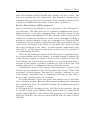
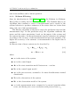
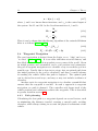
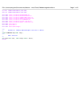
For the fast system a feedback control is developed. Let z denote the
difference between the actual state δ and the desired value arctan(−k1 θ)
z = δ − arctan(−k1 θ)
v
−k1
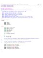
ż = sin(δ) −
θ̇ + ω
r
1 + (k1 θ)2
ż = θ̇ + ω +
−k1
θ̇
1 + (k1 θ)2
v
−k1
) sin(z + arctan(−k1 θ)) + ω
ż = (1 +
2
1 + (k1 θ) r
(5.9)
(5.10)
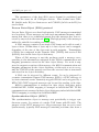
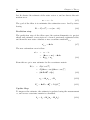
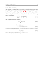
In order to achieve an exponetially stable system we want the following
solution.
ż = −z
(5.11)
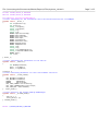
By chosing
k1
v
sin(z + arctan(−k1 θ)))
ω = − (k2 z + (1 +
r
1 + (k1 θ)2
(5.12)
we achieve
v
ż = −k2 z
(5.13)
r
Where = k2rv . Consider τ = vr denoting the smallest time to which the
slow subsystem can reach the goal. Then we have = kτ2 . By choosing
k2 >> 1 the fast subsystem will be sufficiently faster than the slow subsystem.
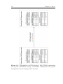
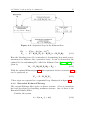
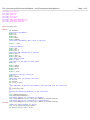
In the original coordinates the control law (5.12) is written as
v
k1
ω = − (k2 (δ − arctan(−k1 θ)) + (1 +
sin(δ))
r
1 + (k1 θ)2
(5.14)
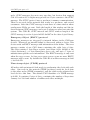
Note that ω is linearly dependent of the speed v of the vehicle. Let R
denote the radius of the turn. Then the curvature of the path is defined
by κ = R1 , which again can be written as κ = ωv . The curvature of the
path from this control law is then
1
k1
κ = − (k2 (δ − arctan(−k1 θ)) + (1 +
sin(δ))
r
1 + (k1 θ)2
(5.15)