Download Part I. Standard HyperCarte Web Application

HyperCarte Web Application
HyperAtlas and HyperAdmin User's Manual
HyperCarte Research Group
Draft
Draft
HyperCarte Web Application: HyperAtlas and HyperAdmin User's
Manual:
HyperCarte Research Group
Abstract
This document provides the minimum information about how to use HyperAtlas and HyperAdmin from the HyperCarte Web Application version 1.0.2.
Draft
Draft
Table of Contents
Introduction ................................................................................................................ vii
1. Overview ................................................................................................................. 1
I. Standard HyperCarte Web Application .......................................................................... 3
2. All users .......................................................................................................... 4
3. Registered users ................................................................................................ 7
II. Standard HyperAtlas ................................................................................................. 9
4. Standard HyperAtlas startup .............................................................................. 11
5. Standard HyperAtlas input dataset ...................................................................... 14
6. Overview ....................................................................................................... 15
6.1. File menu ............................................................................................ 16
6.2. View menu .......................................................................................... 16
6.3. Tools menu .......................................................................................... 18
6.4. Session menu ....................................................................................... 20
6.5. Help menu ........................................................................................... 20
7. MTA parameters ............................................................................................. 22
7.1. An example of multiscalar typologies of regions ......................................... 22
7.2. Setting the Study Area ........................................................................... 22
7.3. Setting the indicators ............................................................................. 23
7.4. Setting the contexts for deviations ............................................................ 24
7.5. The synthesis maps ............................................................................... 25
7.5.1. Ternary synthesis map ................................................................. 26
7.5.2. Dual synthesis map ..................................................................... 27
8. Tools ............................................................................................................. 34
8.1. Review of available maps tabs ................................................................. 34
8.2. Appearances and functions of the mouse cursor .......................................... 35
8.3. Legends, options and explanation tabs ....................................................... 36
8.4. Zoom .................................................................................................. 37
8.5. Report ................................................................................................. 38
9. Standard HyperAtlas Expert Mode ...................................................................... 40
9.1. Lorenz curve and statistical indexes .......................................................... 40
9.2. Equi-repartition map .............................................................................. 41
9.3. Boxplots chart ...................................................................................... 42
9.4. Spatial autocorrelation chart .................................................................... 43
III. HyperAdmin ......................................................................................................... 45
10. Standard HyperAdmin Overview ...................................................................... 47
11. Geometry input .............................................................................................. 48
11.1. The MID file ...................................................................................... 48
11.2. The MIF file ....................................................................................... 49
11.3. Layer of main cities ............................................................................. 52
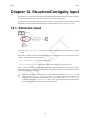
12. Structure/Contiguity input ................................................................................ 54
12.1. Structure input .................................................................................... 54
12.2. Contiguity input (optional) .................................................................... 58
13. Stocks input .................................................................................................. 64
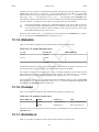
13.1. HyperAdmin input data file format ......................................................... 64
13.1.1. About ...................................................................................... 64
13.1.2. Data ........................................................................................ 64
13.1.3. Default .................................................................................... 65
13.1.4. Label ...................................................................................... 65
13.1.5. Metadata .................................................................................. 66
13.1.6. Provider .................................................................................. 66
13.1.7. RatioStock ............................................................................... 66
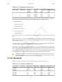
13.1.8. StockInfo ................................................................................. 67
14. Standard HyperAdmin build ............................................................................. 69
A. Annex: when things go wrong... ................................................................................ 71
A.1. Known bugs ................................................................................................ 71
iii
Draft
HyperCarte Web Application
Draft
A.1.1. HyperAtlas is frozen ...........................................................................
A.1.2. Deviations maps update .......................................................................
A.1.3. Multiple boxes appear .........................................................................
B. Annex: acronyms ....................................................................................................
C. Annex: glossary ......................................................................................................
D. Annex: references ...................................................................................................
E. HyperAtlas Application Terms and Conditions of Use ....................................................
F. About ....................................................................................................................
iv
71
72
72
73
74
78
79
80
Draft
Draft
List of Figures
2.1. Standard HyperAtlas License .................................................................................... 4
2.2. Dataset Page .......................................................................................................... 5
2.3. Log in Page ........................................................................................................... 5
2.4. Help ..................................................................................................................... 6
3.1. Registered status menu bar ....................................................................................... 7
3.2. Advanced status menu bar ........................................................................................ 7
3.3. Hyps upload form ................................................................................................... 8
4.1. Security Warning .................................................................................................. 12
4.2. Security Warning: More Information ........................................................................ 12
4.3. Security Warning: Certificate Details ........................................................................ 13
6.1. Standard HyperAtlas frame overview ........................................................................ 15
6.2. Screenshot of the File menu .................................................................................... 16
6.3. Screenshot of the View menu .................................................................................. 16
6.4. Display submenu options: cities layer ....................................................................... 17
6.5. Displayed cities .................................................................................................... 17
6.6. Screenshot of the Tools menu ................................................................................. 18
6.7. Study area creation window .................................................................................... 19
6.8. Study area creation success ..................................................................................... 19
6.9. Map of the new study area ..................................................................................... 20
6.10. Screenshot of the Session menu ............................................................................. 20
6.11. Screenshot of the Help menu ................................................................................. 20
7.1. Study area fields ................................................................................................... 23
7.2. Combination of study area and elementary zoning ....................................................... 23
7.3. Indicators box ....................................................................................................... 24
7.4. Numerator, denominator and ratio tabs ...................................................................... 24
7.5. Contexts box ........................................................................................................ 25
7.6. Deviations maps tabs ............................................................................................. 25
7.7. Synthesis map options ............................................................................................ 26
7.8. Synthesis map tab ................................................................................................. 27
7.9. A deviations synthesis histogram for a regiion ............................................................ 27
7.10. Legend of the dual synthesis map ........................................................................... 29
7.11. Dual synthesis map: red units ................................................................................ 30
7.12. Dual synthesis map: blue units ............................................................................... 31
7.13. Dual synthesis map: yellow units ........................................................................... 32
7.14. Dual synthesis map: final typology ......................................................................... 33
8.1. Details box for the synthesis map ............................................................................. 35
8.2. Options for proportional circles ............................................................................... 36
8.3. Options for deviation maps ..................................................................................... 37
8.4. Spatial zoom slider ................................................................................................ 38
8.5. Screenshot of a generated report .............................................................................. 39
9.1. Expert mode enabled ............................................................................................. 40
9.2. Lorenz curve, statistical indexes and explanations ....................................................... 41
9.3. Equi-repartition map .............................................................................................. 42
9.4. Boxplots chart ...................................................................................................... 43
9.5. Spatial autocorrelation chart .................................................................................... 44
10.1. Standard HyperCarte Workflow ............................................................................. 47
11.1. MIF file header ................................................................................................... 49
11.2. Example of two "Region" entries in the MIF file Data section ...................................... 51
12.1. Number S of needed sheets for n units .................................................................... 63
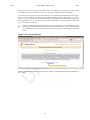
14.1. Dataset information form ...................................................................................... 69
14.2. Successfull build ................................................................................................. 70
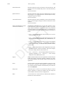
A.1. Java console: stroke shape error .............................................................................. 71
C.1. Mathematical formula of the relative deviation ........................................................... 75
C.2. Ratio .................................................................................................................. 77
v
Draft
Draft
List of Tables
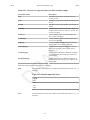
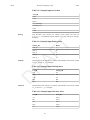
12.1. Overview of expected sheets for data structure input ..................................................
12.2. Sample input Unit sheet ........................................................................................
12.3. Sample input Area sheet .......................................................................................
12.4. Sample input Zoning sheet ....................................................................................
12.5. Sample input UnitSup sheet ..................................................................................
12.6. Sample input UnitArea sheet .................................................................................
12.7. Sample input UnitZoning sheet ..............................................................................
12.8. Sample input Language sheet .................................................................................
12.9. Sample input UnitLanguage sheet ...........................................................................
12.10. Sample input AreaLanguage sheet .........................................................................
12.11. Sample input ZoningLanguage sheet .....................................................................
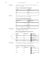
12.12. Overview of expected sheets for contiguity input .....................................................
12.13. Sample input Contiguity sheet ..............................................................................
12.14. Sample input ContiguityLanguage sheet .................................................................
12.15. Sample input Neighbourhood sheet .......................................................................
12.16. Sample input NeighbourhoodLanguage sheet ..........................................................
12.17. Sample input ContiguityZoning sheet ....................................................................
12.18. Sample input ContiguityArea sheet .......................................................................
12.19. Sample input UnitContiguity sheet ........................................................................
12.20. Example of needed sheets number ........................................................................
13.1. V2 sample About sheet ........................................................................................
13.2. V2 sample Data sheet ..........................................................................................
13.3. V2 sample Default sheet .......................................................................................
13.4. V2 sample Label sheet .........................................................................................
13.5. V2 sample Metadata sheet .....................................................................................
13.6. V2 sample Provider sheet .....................................................................................
13.7. V2 sample RatioStock sheet ..................................................................................
13.8. V2 sample StockInfo sheet ....................................................................................
vi
55
55
56
56
56
56
57
57
57
57
58
58
59
59
60
61
62
62
62
63
64
65
65
65
66
66
67
67
Draft
Draft
Introduction
The next chapter, Overview, proposes an overview of a typical Multiscalar Territorial Analysis (MTA)
session with Standard HyperAtlas v2. Then, this document aims at providing an user's manual for the
usage of the following applications:
• Standard HyperAtlas
• HyperAdmin
First of all, please insure that you have carefully read the HyperAtlas Application Terms and
Conditions of Use.
Both previous applications were historically available as standalone applications. They are now available from the Internet and embedded in a Web application whose main pages and use are described
in the first part of this document : Standard HyperCarte Web Application.
HyperCarte Research Group aims at providing projects and applications for interactive cartography.
The projects focus on the development of an easily understood methodology that allows the analysis
and visualization of spatial phenomena, taking into account its multiple possible representations.
Statistical observations of the territory are complex, and one representation, directly linked to a precise
objective, is the result of a combination of different choices which are relative on one hand to the
territories and their geographical scales, to the the statistical indicators on the other hand. This is of
interest for researchers as well as for development policy decision-makers.
Thus, the principal innovative aspect of the HyperCarte project lies on this perspective based on the
popularization of methods coming from spatial analysis such as the fitting of territorial scales, gradients, discontinuities…. This supposes an effort of multidisciplinary cooperation between geographers
and computer scientists in order to create new maps in real time according to the different choices. An
important effort has concerned ergonomics and time of calculus.
Main partners of the HyperCarte research group are:
RIATE [UMS 2414] http://www.ums-riate.com
CNRS UMR 8504 Géographie-Cités [UMR 8504]
http://www.parisgeo.cnrs.fr
LIG-MESCAL
mescal.imag.fr/
[UMR
5217]
http://
LIG-STeamer
steamer.imag.fr/
[UMR
5217]
http://
For more information, please visit HyperCarte Research Group Web site on http://hypercarte.imag.fr.
vii
Draft
Draft
Chapter 1. Overview
As an introduction, this chapter proposes an overview of a typical Standard HyperAtlas v2 session,
describing possible paths of investigation.
Users of the Standard HyperAtlas v1 may remember the typical path of investigation, they were supposed to follow the seven following steps:
1. Choice of area, zoning and indicator of interest (that's to say a ratio)
2. Visualization of the ratio and (eventually) visualization of numerator and denominator without
transformation
3. Analysis of inequalities at large level
4. Analysis of inequalities at medium level
5. Analysis of inequalities at local level
6. Synthesis of inequalities at large, medium and local level
7. Export of results towards a report
Of course, users are free to develop their own paths of investigation, and we can imagine different
types of scenarios where users do not follow steps 1 to 7, but they adopt different strategies.
Let's now consider the following examples to demonstrate the benefits of a Multiscalar Territorial
Analysis approach thanks to Standard HyperAtlas:
• Example 1
A stakeholder interested in the reform of structural funds after 2013 will probably use a path of
investigation following the type (1)=>(3)=>(7) that will be repeated many times in order to test
various scenario of allocation of funds. For example, what happens if:
• NUTS2 is replaced by NUTS3?
• GDP pps is replaced by GDP in Euro?
• the threshold of 75% of EU mean is replaced by 80%?
• Turkey joins EU?
• etc.
• Example 2
A local decision maker mainly interested in its region may use a path of investigation following
the type (1)=>(6)=>(Save map), if the objective is to quickly extract three figures describing the
situation of the regions at European, National and Local levels for a given criteria. He/she can then
decide to click on other regions in order to benchmark its situation with neighbouring areas, or to
identify other regions with the same strength and weaknesses. He/she can also decide to modify the
indicator and to explore the strength of weaknesses of his/her region for various criteria, GDP/inh,
unemployment, accessibility, ageing, etc.
• Example 3
A spatial economist interested in economic convergence may decide to examine the situation of
regions according to vertical contexts (e.g. belonging of region to a state, an INTERREG area) and
horizontal contexts (e.g. difference between a region and its neighbours for different thresholds of
1
Draft
Overview
Draft
contiguity or distance). He/she will therefore follow the expected steps (1) to (7), but he/she will
probably introduce loops in the steps (4) and (5) in order to explore different variants of vertical and
horizontal context. The loop (1)=>(5) will for example provide answer on question like the GDP/
inh. Of course, the region of Budapest is greater than the neighbours for a distance of one hour by
road, but what happens for a distance of two hours on a truck? Four hours? etc.
Having established that different users will not pay equal attention to the different functions offered
by HyperAtlas, we can also suspect that expert users will expect more sophisticated functions than
non-expert users, who will be on the contrary reluctant to enter into complex indicators or results.
Considering these different types of users, Standard HyperAtlas v2 provides an expert mode (see
Standard HyperAtlas expert mode chapter), opened on request by the user (expert users or curious). In
summary, the expert mode provides the following tools that complete the typical path of investigation:
• Equi-repartition maps, one per context, for Large, Medium and Small (local) levels
• Lorenz curve and statistical indexes (Gini index, Hoover index, coefficient of variation, ...)
• Boxplots
• Spatial autocorrelation chart
2
Draft
Draft
Part I. Standard HyperCarte
Web Application
This part describes the main pages of the Standard Web Application embedding the Standard HyperAtlas and
Standard HyperAdmin applications.
Some pages are only available to registered users, hence the following dedicated chapters:
• pages for any users are described in All users chapter;
• pages for registered users are described in Registered users chapter.
Draft
Draft
Chapter 2. All users
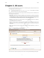
First access to the Web Application invites the user to read and accept the conditions and terms of use
of the HyperAtlas, as shown on Figure 2.1.
On following screenshots, the http://127.0.0.1:8080/ is the IP address of the alpha
application that has been used to create this document..
The links on the top right menu bar of the page provides the main topics that are available for this
Standard HyperCarte application:
• HyperAtlas: when the user accepts the conditions of use (see Figure 2.1) , he/she can execute the
Standard HyperAtlas v2 applet. This applet allows then to perform a multiscalar territorial analysis
on a default dataset (currently: Economy and Social Affairs). Please consult Standard HyperAtlas
part of this document for further information on how to use Standard HyperAtlas.
• Dataset: for further analysis, this page provides a list of available datasets that can be loaded by
the Standard HyperAtlas v2 (Figure 2.2).
• Log in: as shown on Figure 2.3, this page provides a form for registered users who can log into the
application in order to access advanced features. Registered users are invited to consult Registered
users section.
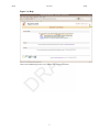
• Help: displays links to the user's manual and the version of the Web Application, as shown on
Figure 2.4.
Figure 2.1. Standard HyperAtlas License
The license must be read and accepted by the user before accessing the Standard HyperAtlas applet.
4
Draft
All users
Draft
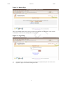
Figure 2.2. Dataset Page
The list of available datasets on this page provides various thematics and study areas. Click the name
of the dataset to load the associated hyp file into HyperAtlas.
Figure 2.3. Log in Page
"Forgotten login?" and "Not registered yet?" links are not implemented yet. Just check a "missing feature" page is returned on clicking these links.
5
Draft
All users
Figure 2.4. Help
Links to the Standard HyperCarte User's Manual and version information.
6
Draft
Draft
Draft
Chapter 3. Registered users
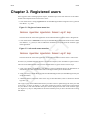
Once logged in with a valid login/password pair, available topics in the main menu bar of an authenticated session depend on the current user's status:
• a user whose status is simply registered can use Standard HyperAdmin integration tool to generate
new dataset .hyp files.
Figure 3.1. Registered status menu bar
The main menu bar of the Web application for an authenticated user whose status is "Registered".
• a user whose status is advanced can not only use Standard HyperAdmin but he/she can also submit
new datasets (.hyp files) in order to make them available to everybody from the "Dataset" page
of the application.
Figure 3.2. Advanced status menu bar
The main menu bar of the Web application for an authenticated user whose status is "Advanced".
Of course, any available feature to all users (see All users chapter) is also available to registered users.
The tools of the authenticated session can be summarized as a typical scenario in three steps:
1. create a new dataset: as building a new dataset is quiet an advanced subject, the detailed use of
Standard HyperAdmin is further described in the HyperAdmin part of this document.
2. check your newly created dataset hyp file from Standard HyperAtlas (see Standard HyperAtlas part
of this document)
3. submit the dataset ("advanced" status users only) as described below, How to submit new dataset
hyp files? [7]
The "hyp(s)" page of the authenticated session provides a form to upload an hyp file from your disk
to the server, as shown on Figure 3.3. The form requires the input of a name and of a description
for your dataset. This name and this description will be displayed in the table of the "Dataset" page
(see Figure 2.2), they are independant of the name and description you have entered while creating
this dataset.
7
Draft
Registered users
Draft
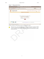
Figure 3.3. Hyps upload form
Requires an hyp file, a name and a description for the dataset to be added.
Please test your hyp file with Standard HyperAtlas before submitting it, as it will be available
to all users. The provided management feature currently only allows to add datasets, not to
remove available ones. This "remove" feature can currently only be performed by the administrator of the server.
8
Draft
Draft
Part II. Standard HyperAtlas
Standard HyperAtlas is a tool for Multiscalar Territorial Analysis: several indicators on the basis of the ratio of
two initial geographical indexes can be derived, according to different spatial contexts.
Multiscalar Territorial Analysis is based on the assumption that it is not possible to evaluate the situation of a given
territorial unit without taking into account its relative situation and localization. Regions belong to territorial and
spatial systems. Indeed, from a policy point of view and in a social science perspective, contrasts and gradients are
of much more interest than absolute values. Furthermore, aggregating and disaggregating territorial units allow to
see how local values add up to form territorial contexts and regional positions.
Whatever the indexes used for political decisions, they have to be evaluated in relative terms. This may be done
according to various territorial contexts. Thus one spatial organization may be examined from three different
viewpoints that are three territorial contexts. They are differentiated according to the scale of political intervention
or action they are referring to and that have a sense for the questioning: a global one, a medium one and finally
a local one. Thus what is represented is the deviations to the three reference values associated to these different
levels.
Let us take the example of the European union as a set of 25 countries, at the level of the region (NUTS2 for
instance), and let the observed index be the wealth per resident in the regions (GDP/inh.). It is possible with
Standard HyperAtlas to consider the level of wealth of the regions relatively to three territorial contexts, and not
only from an absolute point of view. The chosen contexts may be for instance respectively:
1. the whole European Union;
2. the country;
3. the neighborhood defined by contiguous regions.
Standard HyperAtlas proposes for such an indicator a set of maps and charts that will be furthermore described
in MTA parameters and Tools:
• First maps show the selected study area, both the parent distributions as disc maps (here, wealth and population)
and their ratios, that is to say the chosen index’s one.
• Then, three maps show the relative deviations to the three chosen contexts as choropleth maps. For the above
example: the deviation of a region to the European reference area, the deviation of a region to its national
reference area, and in the third place the deviation of a region to the local reference area.
• Then, two synthesis maps allow to evaluate the different combinations of the three previous relative deviation
maps.
• More advanced users are also provided a set of new tools like the maps of redistribution, the Lorenz curve and
a chart of spatial autocorrelation.
Here are some political justifications about the contextual and multilevel mapping, based on the European
example:
• The first map where the referent context is the global one is the classical way of mapping an index when
the chosen context is the studied area. The values of the indices are converted into a global index.
• The second map, corresponding to the intermediate level, her the national one, is very important to
combine with the previous one. Indeed, many contradictions can appear between the two levels, with
important political consequences.
• The third one is based on the local differential between one region and the neighbouring ones according to various criteria of proximity (contiguity, time-distance). According to recent research in the field
of spatial economy and regional science, those local advantages/handicaps appear to be of crucial importance for the regional cohesion because they are strongly connected with the action of economic or
social actors.
Draft
Draft
• The multiscalar approach proposed to evaluate the same index at various scales. In terms of territorial
cohesion, it is indeed very important to evaluate the level of development of a region according to at
least three levels.
Draft
Draft
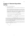
Chapter 4. Standard HyperAtlas
startup
Before starting Standard HyperAtlas:
Standard HyperAtlas is available on-line from the Standard HyperCarte Web Application (see
Figure 2.1 in All users chapter).
Based on the Java technology applet, Standard HyperAtlas requires a standard Web browser
and a correctly installed Java Runtime Environment (JRE) plugin. This JRE is available by
default on all standard Web browsers, whatever the platform is. A version 1.6 or upper of the
JRE is advised, when available for your operating system. Nevertheless, on Mac OS X 32
bits platform, the user can currently (2010) not select a more advanced version than 1.5, but
Standard HyperAtlas is compatible with this version. So, please update your environment to
get at least this version 1.5 of the JRE, but prefer the 1.6 when possible.
For more information about your JRE, please consult the following links (last visit: 20101228):
• Verify Java version [http://www.java.com/en/download/installed.jsp]
• How do I enable java in my web browser? [http://www.java.com/en/download/help/
enable_browser.xml]
• Mac OS X users: Java Frequently Asked Questions [http://developer.apple.com/java/faq/]
Before starting the application, the user is warned that the HyperAtlas Applet is about to be run without
the security restrictions that are normally provided by Java. Indeed, Standard HyperAtlas is allowed
to read-write on the user's disk to load a personal .hyp file or to write an html report for example. To
overcome the default behaviour of Java Applets that are not allowed to write on the user's disk, the
Standard HyperAtlas applet has been signed with a CNRS-2 standard certificate (CNRS is an acronym
for Centre National de la Recherche Scientifique).
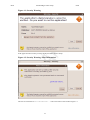
Thus, the security warning window (Figure 4.1) which is opened before the startup of the application
is expected. The user can insure about the content he is about to execute by opening the details of the
certificate, as shown on figures Figure 4.2 and Figure 4.3.
11
Draft
Standard HyperAtlas startup
Draft
Figure 4.1. Security Warning
JVM Applet execution security warning displayed window before startup.
Figure 4.2. Security Warning: More Information
The user has clicked the More information... link on the bottom of the window Figure 4.1
12
Draft
Standard HyperAtlas startup
Draft
Figure 4.3. Security Warning: Certificate Details
The user has clicked the Certificate details... link on the bottom of the window Figure 4.3
Once the user has clicked the Run button on the security warning popup window, the Standard HyperAtlas applet begins to load a dataset. Depending on the speed of this loading, a splash screen icon
may appear a few seconds:
13
Draft
Draft
Chapter 5. Standard HyperAtlas input
dataset
The datasets provided by geographers are serialized in a convenient format for Standard HyperAtlas
to a binary file named with the .hyp extension (example: Europe_2007.hyp). As a convention,
these Standard HyperAtlas dataset input files will be now called hyp files.
A complete description of the Standard HyperAtlas integration tool, named Standard HyperAdmin, is available from the HyperAdmin part of this document.
Standard HyperAtlas is designed so it can load any dataset serialized as an hyp file. From the "HyperAtlas" menu item of the HyperCarte Web Application main menu bar, once the user has accepted
the terms and conditions of use (see Figure 2.1), the Standard HyperAtlas loads a default dataset:
Rhône-Alpes.
The user can also load a dataset hyp file from his disk via the "File-Open" menu item of the application.
Customized datasets for various topics are also available from the "Datasets" page of the Web Application, see Figure 2.2.
14
Draft
Draft
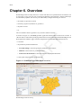
Chapter 6. Overview
Standard HyperAtlas is totally interactive. It works with three sets of parameters that are linked to one
or more maps. At any time, the user can change the different input parameters, and the linked maps
are immediately updated. The user may also individually configure each map, for instance:
• the number of equivalence classes
• statistical progression (arithmetic or geometric)
• the pallet of colors
• etc.
This set of features allow to generate a very accurate collection of maps.
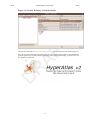
As shown on Figure 6.1, StandardHyperAtlas Applet fills the full width of the browser window. A
"Back to dataset" link at the top of the page allows the user to be redirected to the Standard HyperCarte
Web Application "Dataset" page. The main components of the Standard HyperAtlas frame are:
• a menu bar
• the parameters panel threefold boxes:
• Area and Zoning to select the geometric parameters of the analysis;
• Indicator to select stocks or pre-defined ratios;
• Contexts for the deviations to select the references of computed deviations.
• a main panel composed of the generated maps
Figure 6.1. Standard HyperAtlas frame overview
Standard HyperAtlas at startup..
15
Draft
Overview
Draft
Following sections first detail each item in the menu bar of the application.
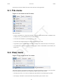
6.1. File menu
Figure 6.2. Screenshot of the File menu
This menu allows:
• to open a new dataset hyp file from your disk or from an eventual known URL (Unified Resource
Locator) to an hyp file located at a server on the Internet;
• to save the current dataset to your disk as an hyp file;
• to save the current displayed tab as an image (PNG) file to your disk;
• to generate a report in HTML format, including an image each current tab of the current analysis.
• to be redirected to the Web Application Dataset page in order to load another on-line dataset (see
Figure 2.2)
.
6.2. View menu
Figure 6.3. Screenshot of the View menu
This menu concerns the appearance of the maps. It provides menu items to zoom in, zoom out and to
choose the different panels that can be displayed as different parts of the window:
• the "Map only mode - F11" allows to display the map frameset as wide and high as possible;
• the "Display - Parameters" menu item makes the parameters panel visible or note.
16
Draft
Overview
Draft
Depending on the current loaded dataset, the "Display" submenu may also include an additional checkbox item as shown on the Figure 6.4. This checkbox allows the user to display or hide the main cities
over the map. By default, if the dataset provides such a layer, it is checked.
Figure 6.4. Display submenu options: cities layer
On this screenshot, the loaded dataset embeds the main cities. The "Display" menu allows to hide or
display this additional layer.
When the Display-Cities menu item is enabled, cities are displayed over the maps as black squares, as
shown on Figure 6.5. Note that for ergonomy reasons, to avoid overlapping between cities labels, the
names of the cities are not displayed over the map. Nevertheless, a tooltip appears when the mouse
comes over a square.
Figure 6.5. Displayed cities
Cities are represented as black squares. The name of the city appears when the mouse moves over
a square.
17
Draft
Overview
Draft
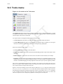
6.3. Tools menu
Figure 6.6. Screenshot of the Tools menu
The Popup Freeze menu item has been available since HyperAtlas v2. This functionnalitiy is usefull
to compare several maps or charts: clicking on this menu item, a popup window is opened, displaying
a frozen image of the current visisted tab.
Two options allow to manage the behavious of the mouse cursor:
• The Turn Pan menu item allows to enable the moves of the maps inside the window.
• The Turn Histogram menu item is only enabled for the synthesis map, it displays for each region
the three contextual deviations (see synthesis as an histogram [27] paragraph)
Other tools available on this menu:
• Create a study area menu item is described below.
• Enable expert mode" menu item is described in Standard HyperAtlas expert mode chapter of this
document.
• Borders options: use this item to choose the colors of borders of territorial units for example.
• Language: this menu item opens a dialog box that provides the list of available languages for the
interface of the frame. The internationalization feature is currently available in english, french and
romanian. The default language at startup depends on the locale of your system, english by default.
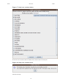
This version 2 of Standard HyperAtlas allows to define a new study area. On clicking this menu item,
the user is invited to enter a name for his/her new study area and to select the top-levels units (as a
rule, countries) that will compose this study area.
Figure 6.7 shows the example of a user who wants to define the benelux study area. He/she selects
Belgium, Luxembourg and Nederlands units then clicks the "Submit" button. Figure 6.8 shows
the information message that is displayed when the creation is successfull. The benelux parameter
is now available from the Study Area combo box of the parameters panel. Figure 6.9 shows that
interactive maps have been consequently updated on selecting this new study area.
18
Draft
Overview
Figure 6.7. Study area creation window
Provides the list of countries and a text field to enter a name for this new study area.
Figure 6.8. Study area creation success
Infomation message.
19
Draft
Draft
Overview
Draft
Figure 6.9. Map of the new study area
Selected new study area.
6.4. Session menu
Figure 6.10. Screenshot of the Session menu
This menu allows to save the parameters of the current analysis to an Standard HyperAtlas XML file
on your disk.
In the case when you already saved such a file, this menu allows to load your previous session parameters.
A session parameters file is specific to a dataset. An error occurres if you try to load a session
parameters file that was built while using another dataset.
6.5. Help menu
Figure 6.11. Screenshot of the Help menu
20
Draft
Overview
Draft
This menu provides the following items:
• Help (F1): opens a new browser window to the on-line user's manual (see Figure 2.4).
• About dataset opens a popup window displaying metadata of the current dataset (author, creation
date, version).
• About displays the current version of the software. Please note this version when reporting an
eventual bug as described in Annex: when things go wrong.
21
Draft
Draft
Chapter 7. MTA parameters
This section focuses on how to set the parameters for a Multiscalar Territorial Analysis
(MTA [73]). As its title suggests it, the next section (An example of multiscalar typologies of regions) first describes the main concept of such an analysis. Please read it in order to efficiently benefit
of the provided tools by Standard HyperAtlas v2.
Some screenshots of this chapter were performed with a previous version of HyperAtlas.
Though the graphical user interface has been updated since this version, the concepts remain
the same.
7.1. An example of multiscalar typologies of
regions
Taking account the European level as an example, this section focuses on the importance of considering the multiscalar typologies of regions in political decisions.
When the policymakers want to build political scenari or when they want to evaluate propositions of
structural funds, they need to get a synthetic view on the situations of regions which depend on the
various territorial contexts.
The question of perequation (transfer from “advanced” to “lagging” region) is very sensible and it is
important to propose a complete view of the scales where those perequation processes can take place,
according to the principle of subsidiary.
As an example, we analyse how the picture of “lagging” regions is modified when the previous criterion of Objective 1 (less than 75% of the mean value of GDP) is applied simultaneously at three
scales: European, national and local.
Simultaneously, it is possible to propose a typology of “advanced regions” based on the symmetric
criteria of more than 133% of the mean value of GDP at those three scales.
According to this methodology, it is possible to demonstrate that very few regions are “lagging at
all scales” and “advanced at all scales”. Many are in more complex situations, like certain regions
of Switzerland or Norway which are “advanced” at European scale, but they are “lagging” at their
national or local scales.
Reversely, the metropolitan regions of candidate countries are very often “lagging at European scale”
but “advanced at national and local scales”.
7.2. Setting the Study Area
The setting of the study area should be the first step of any analysis. Setting the basis of the study can
be done by answering the following questions:
• which spatial extension (area) and for which geographical level?
• which division will be the elementary zoning?
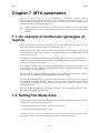
As shown on Figure 7.1, these two parameters have to be selected in the two respective pop up lists.
The different propositions are internal and come from the a priori implementation.
22
Draft
MTA parameters
Draft
Figure 7.1. Study area fields
• Study Area shows the spatial extension that will be mapped.
• Elementary zoning shows the set of elementary units that will be studied.
Figure 7.2 illustrates two possible combinations. The selected area is mapped when the chosen elementary zoning is drawn.
Figure 7.2. Combination of study area and elementary zoning
These two maps were extracted from the "Area and Zoning" tab of the application with following
settings:
Study Area
Elementary Zoning
Map on the left
European Union 15
NUTS 0
Map on the right
New member states 12
NUTS 3
7.3. Setting the indicators
Standard HyperAtlas only works with size variables (that is to say that only variables that may be
aggregated at upper level by sum), and proposes a multiscalar cartography of the ratio for two size
variables in order to set the studied ratio. The user can combine every couple of these types of variables
in the “Indicators” box, by choosing each of them in the associated select boxes as shown on Figure 7.3.
23
Draft
MTA parameters
Draft
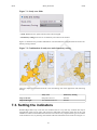
Figure 7.3. Indicators box
This box provides three select boxes to choose indicators. The user selected the Density item in
the Ratio select box:
• Numerator is set to Population in 2003
• Denominator is set to Area in km2
• Ratio: depending on the chosen dataset (the hyp file), selecting a ratio may implie the auto-selection
of the numerator and denominator fields values.
Three maps are respectively linked to these choices, under three different tabs (see Figure 7.4). The
maps for the numerator and for the denominator (size variables) are represented with proportional
circles. The ratio map is shown with colored units, according to the ratio value. The number of classes
and their associated colors (the pallet tool) can be can be set in the "Option" tab of the ratio map.
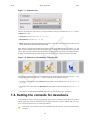
Figure 7.4. Numerator, denominator and ratio tabs
The three associated tabs to the chosen indicators are represented here for the study area EU 15 (15
countries in Europe) with the NUTS 0 value (countries) for the elemetary zoning:
• the image on the left shows the Numerator map within its associated tab, here, the population
in 2003
• the image in the center shows the Denominator map within its associated tab, here, the area in
km2
• the image on the right shows the Ratio map within its associated tab, here, the density.
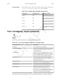
7.4. Setting the contexts for deviations
As described in various contexts [9] paragraph, the user has to define the three territorial contexts
which respectively set three different levels of spatial observation: global, medium and local. Figure 7.5 shows the select boxes to set these parameters.
The names of the references have been updated since the previous versions of Standard HyperAtlas:
24
Draft
MTA parameters
Draft
• Global has been renamed General;
• Medium has been renamed Territorial;
• Local has been renamed Spatial.
Figure 7.5. Contexts box
The "Contexts" box allows to set three references for their associated deviations: general, territorial
and spatial contexts.
The general context may be the whole chosen study area. In such a case, the associated map will be
the same as the associated map to the ratio itself. So, the user may choose another general context or
a reference value. For instance, in the example of the EU, even if the study area is the 29 potential
countries, it may be of interest to observe the spatial differentiations according to another global reference, for instance the global value associated to EU15. For this level, the user may also exogenously
enter a value. By default, this value has first been set to the value of the global area.
The territorial context, on the other hand, has to be a geographical zoning that is an aggregation of
the “elementary zoning” that was previously chosen.
The spatial context shows which proximity relation will be the basis of the neighborhood’s definition
for each elementary unit. That is usually “contiguity”, but it may also be a relationship based on
distances since they have been introduced in the hyp file (units that are less than X kilometers far from),
or time-distances. Then, each elementary unit value will be compared to the value of its neighborhood.
A set of three maps are linked to these choices (Figure 7.6). The values of the deviations are transformed into global indexes 100. Thus, values may be interpreted in terms of percentage to the reference value. The maps are drawn with double progression frame centered on 100, in order to highlight
the regions that are under the reference value (100), and the ones that have upper values.
Figure 7.6. Deviations maps tabs
These screenshots show the three deviations maps tabs for chosen contexts: general deviation on the
left, territorial deviation in the center and spatial deviation on the right.
7.5. The synthesis maps
One synthesis map was already available in the previous version of Standard HyperAtlas, based on
three levels and one treshold, it is described in Ternary synthesis map. A new synthesis map has been
added to the application since the version 2.0: see Dual synthesis map.
25
Draft
MTA parameters
Draft
7.5.1. Ternary synthesis map
The three relative positions about contexts are summarized in one synthetic map. The elementary units
are classified in eight classes according to their three relative positions.
In order to reduce the whole combinatory of possible cases, from the "Options" tab close to the synthesis map (Figure 7.7), the user must specify which point of view he wants to focus on: the first "Criterion" parameter shows whether the point of view is to underline the regions whose ratio is greater
than, or to underline the contextual values, by selecting less than. This choice depends on the studied
indicator (see An example of multiscalar typologies of regions section). For instance high values of
unemployment rates point out different types of regions than high values of an indicator of resources.
According to which regions have to be differentiated (lagging ones or wining ones), the user must
chosse the point of view of the synthesis. Then, the user can choose the threshold percentage.
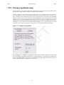
Figure 7.7. Synthesis map options
The map on Figure 7.8 illustrates the eight different configurations of relative position, according to the
three previously chosen contexts and parameters. The legend tab gives for each class the descriptions
of the contextual positions. The last class (in white) gather the regions that are not concerned by the
chosen comparative criterion whatever the contexts are.
26
Draft
MTA parameters
Draft
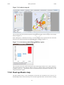
Figure 7.8. Synthesis map tab
This screenshot shows the synthesis map tab for the contexts that were chosen in the previous example
shown on Figure 7.6.
When “Histogram” is enabled (see Section 6.3 section), the user may represent the three contextual
deviations of a selected (clicked) region as an histogram as shown on Figure 7.9.
Figure 7.9. A deviations synthesis histogram for a regiion
This screenshot shows the synthesis histogram of the clicked region named OUEST (West of France).
The general deviation of this region is relative to the UE29 general context. The territorial deviation
is relative to the NUTS 0 hierarchical context, the spatial deviation considers the contiguity, e.g. the
neighborhood of this region.
7.5.2. Dual synthesis map
The dual synthesis map is a new cartographic tool that has been introduced in the version 2.0 of
Standard HyperAtlas. It aims at showing via a chromatic legend the status of territorial units on taking
27
Draft
MTA parameters
Draft
into account two chosen deviations. This section describes the synthetis opportunity that is offered to
analysts thanks to this tool.
The legend of the dual synthesis map shown on Figure 7.10 is composed of four main quarters. The
values on both axis range range from 0 to 200% and they represent the percentages of a deviation of
a territorial unit relatively to a context of reference. The user is invited to select in an options tab the
contexts of deviations to be considered for both axis (among the general, the territorial or the spatial
context).
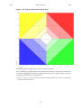
Let's consider the following example: the general deviation has been chosen for the horizontal axis and
the spatial deviation for the vertical axis. The four main colors of the legend represent the following
cases:
• yellow: the global deviation (X axis) is lower than 100% (the average pivot value) and the spatial
deviation (Y axis) is upper 100%
• red: both deviations are upper 100%
• blue: both deviations are lower than 100%
• green: the global deviation (X axis) is upper than 100% and the spatial deviation is lower than 100%
Note that the more far from the value 100 the current deviation is, the more intense the color is. Hence
a white square in the middle of the legend: this range of values show the territorial units whose both
deviations are around the average, 100.
28
Draft
MTA parameters
Draft
Figure 7.10. Legend of the dual synthesis map
Graduations and quarters of the dual deviation synthesis map legend.
Let's consider now a concrete example on how the dual deviation map can help analysts: the following
screenshots decompose as four steps the synthesis about the situation in 2010 according to the European and National averages of unemployement:
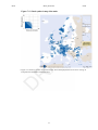
• Figure 7.11 shows in red the territorial units whose unemployement rate is above average both at
European and National levels:
29
Draft
MTA parameters
Draft
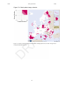
Figure 7.11. Dual synthesis map: red units
• Figure 7.12 shows in blue the territorial units whose unemployement rate is under average both at
European and National levels:
30
Draft
MTA parameters
Draft
Figure 7.12. Dual synthesis map: blue units
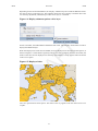
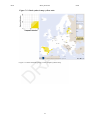
• Figure 7.13 shows in yellow the territorial units whose unemployement rate is above average at
European level and under at National level:
31
Draft
MTA parameters
Figure 7.13. Dual synthesis map: yellow units
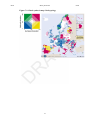
• Figure 7.14 shows the final typology on the complete synthesis map:
32
Draft
Draft
MTA parameters
Figure 7.14. Dual synthesis map: final typology
33
Draft
Draft
Draft
Chapter 8. Tools
This section deals with the available tools in the application to work with the maps.
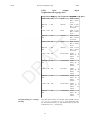
8.1. Review of available maps tabs
First of all, let's review the available maps tabs and their main focuses:
Area and zoning
This map shows the chosen study area and elementary zoning.
Numerator
This map shows the chosen study area and elementary zoning.
Denominator
This map shows the value of the chosen denominator indicator for
each unit of the elementary zoning.
Ratio
This map shows the distribution of the ratio (numerator/denominator) over the units of the elementary zoning.
General deviation
This map proposes the relative perspective of the distribution of
the ratio over the units of the elementary zoning: each absolute
measure is put in relation with a reference value. The reference
value is common for the whole area. The index value is 100 when
an elementary unit has exactly the same value than the reference
value or area. It is 200 when the elementary unit measure is twice
the measure of the reference area, it is 50 when this is half the
measure of the reference area.
Territorial deviation
This map proposes the relative perspective of the distribution of
the ratio over the units of the elementary zoning: each absolute
measure is put in relation with the value of its upper unit in the
reference zoning. The index value is 100 when an elementary unit
has exactly the same value than its reference unit. It is 200 when
the elementary unit measure is twice the measure of the reference
unit, it is 50 when it is half the measure of the reference unit.
Spatial deviation
This map proposes the relative perspective of the distribution of
the ratio over the units of the elementary zoning: each absolute
measure is put in relation with the value of its neighborhood, as
defined by the local reference. The index value is 100 when an
elementary unit has exactly the same value than its neighborhood.
It is 200 when the elementary unit measure is twice the measure of
its neighborhood, it is 50 when it is half the measure of its neighborhood.
Synthesis
This map proposes a synthesis of the different perspectives by
considering the three different contexts. The synthesis is based on
a deviation threshold, either by upper values or by lower value.
These parameters depend on the meaning of the ration and they
must be chosen by the user. Then, a typology of the regions which
check the condition for at least one context is performed.
34
Draft
Tools
Draft
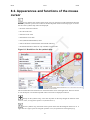
8.2. Appearances and functions of the mouse
cursor
At any moment, the position of the mouse cursor on the map provides information about the
elementary unit that it points. The content of the table depends on the current map, Figure 8.1 shows
the case of the synthesis map where are displayed:
• the name of the territorial unit
• the code of this unit
• numerator stock value
• denominator stock value
• ratio (numerator/denominator) value
• relative deviations values based on the selected references
• the absolute deviation values are only available in expert mode
Figure 8.1. Details box for the synthesis map
This screenshot shows the "Details" box on the left bottom corner of the application. The user's mouse
is over the Guyane. Associated computed values to this unit are displayed in the box.
Except for the synthesis map, a left click anywhere on the map changes the function of the
cursor to “Pan”, as long as this option is on (see Section 6.3).
On the synthesis map, the "hand" mouse pointer shows that the histogram function is on. A
right click on a region opens its histogram synthesis view (see synthesis as an histogram [27]).
35
Draft
Tools
Draft
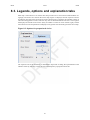
8.3. Legends, options and explanation tabs
Each map is associated to a set of three tabs that provide tools to control and to understand the cartography. The choices are valid for the current map. Figure 8.2 displays each the "Options" tabs for
an indicator map (that shows proportional circles) while Figure 8.3 displays the available options on
a deviation map (palett of colors). The user may also set the thresholds for each class. The "Legend"
tab displays the bounds of the classes (left), the number of items for each of them (right), and the
associated color. The "Explanation" tab displays some general notes about the goal of the current map.
Figure 8.2. Options for proportional circles
The "Options" tab of the numerator or denominator maps aims at setting the representation of the
indicator values by selecting a color, the size and transparency of proportional circles.
36
Draft
Tools
Draft
Figure 8.3. Options for deviation maps
The "Options" tab of the deviation maps aims at setting the representation of the deviation by selecting:
• the palett of colors, that can be reversed
• the number of classes, between two and ten classes
• the progression:
• arithmetic for classes with an equal amplitude, better choice when the distribution is symmetric
around 100.
• geometric for classes with an increasing amplitude
• the thresholds, that can be edited for each class
8.4. Zoom
It is possible to zoom in/out a map, either on clicking the "View - Zoom" menu items, by using the
cursor on the left side of the map or by moving the mouse scroller over the map.
Please note:
• the available zoom levels depend on the selected elementary zoning parameter: reduced
zoom factor for high levels, maximized at lowest level;
• any zoom factor update or pan move are applied to every map;
• the scale of the map is consequently updated.
37
Draft
Tools
Draft
Figure 8.4. Spatial zoom slider
This screenshot shows the scale, the pan buttons and the zoom slider.
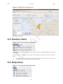
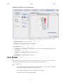
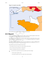
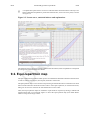
8.5. Report
The user can save his current whole collection of maps with the associated rough data and deviations
by selecting the "File - Build Report" menu item from the menu bar.
By selecting this menu item, the user is invited to select a directory on his/her disk where the report
will be generated as a set of HTML page (index.html and eight PNG image files (one image per
map: map0.png, map1.png, to map7.png).
For example, if the user selected his /home/toto/my_hyperatlas_report/ directory as target directory, he/she may open the saved report from a web browser by selecting the /home/toto/my_hyperatlas_report/index.html file.
The generated report may be divided in the three-fold:
• the introduction shows the space area, chosen indicators and contexts
• the list of maps for these parameters as images files
• the table of generated results for these parameters
In expert mode, the generated report also includes expert tabs as images:
• the three equi-repartition maps
• the tab showing the Lorenz curve and the main statistical indexes
38
Draft
Tools
Draft
• the boxplots chart
• the spatial autocorrelation chart
Figure 8.5 shows an extract of the generated table of results, including all values for all units as they
can be seen on the "Details" box (see Figure 8.1)
Figure 8.5. Screenshot of a generated report
This screenshot shows an extract of the generated report index.html file that has been opened by
in web browser. This image shows the last map (synthesis) and the start of the table that includes all
results.
39
Draft
Draft
Chapter 9. Standard HyperAtlas
Expert Mode
This chapter describes a set of tools that have been integrated since the version 2 of Standard HyperAtlas. As this set of cartographic and statistic tools are mainly designed for more advanced users, they
are not available by default at the startup of the application. In order to keep the application easy to
use for not so advanced users, this set of tools must be enabled on clicking the Enable expert mode
menu item of the "Tools" menu, shown on Figure 6.6.
Graphically speaking, enabling the expert mode adds six new tabs to the eight available tabs in default
standard mode:
• three tabs for equi-repartition maps (respectively for large/medium/small contexts of reference),
they are described in Section 9.2 section.
• a tab showing a Lorenz curve and a table computing relevant statistical indexes. This feature is
described in Section 9.1 section.
• a tab showing a chart of boxplots, described in Section 9.3 section.
• a tab showing a spatial autocorrelation chart, described in Section 9.4 section.
In order to distinguish the default mode tabs and the expert mode tabs, expert tools tabs titles backgrounds are displayed with a golden colour. Enabling the expert mode automatically enables and displays the "equi-repartition" map for the large context, the list of tabs is shown on Figure 9.1.
Figure 9.1. Expert mode enabled
Default mode set of tabs is added six new tabs when enabling the expert mode.
Depending on the operating system, the Java Runtime Environment version (1.5 or upper is
required) and the user's browser, the display may differ. For example, under the Mac OS X.5
operating system with a JRE 1.5, the tabs are embedded in a scrollable list.
9.1. Lorenz curve and statistical indexes
The map of large deviation provided by Standard HyperAtlas is a general measure of disparities for a
given variable Z which is the ratio between two stocks X and Y. This estimation of general disparities
can be further analysed using various econometric indexes that have been added in Standard HyperAtlas v2 expert mode:
• the Lorenz curve typically presents the cumulative proportion of population and resource when
starting from regions with lowest resource per inhabitant.
• the Gini Coefficient is a summary of the Lorenz curve measuring the global amount of disparities:
it is equal to the area located between the Lorenz Curve and the diagonal (perfect-equality)..
• the Hoover index, also called Disparity index, is another summary of the Lorenz Curve, as it is equal
to the maximum distance between Lorenz Curve and diagonale.
• The Coefficient of Variation is simply equal to the ratio between standard deviation and average
of the considered ratio Z.
40
Draft
Standard HyperAtlas Expert Mode
Draft
A complete description of the Lorenz curve and of the main statistical indexes is directly available in a dedicated "Explanation" panel of the statistical box, close to the curve panel, as shown
on Figure 9.2.
Figure 9.2. Lorenz curve, statistical indexes and explanations
This tab shows the Lorenz curve, a table of main statistical indexes, and an "Explanations" titled panel
providing some information for each feature.
9.2. Equi-repartition map
The equi-repartition maps indicate which process of redistribution should be realized in absolute terms
in order to achieve convergence, at European, national or local levels.
The equirepartition map is a bi-color discs map showing an absolute deviation. It examines how much
amount of the numerator should be moved in order to reach equi-repartition, for each territorial unit,
taking into account as a reference the selected deviation context value.
Thus, three equi-repartition maps are available in expert mode for respectively the large, medium and
local deviations tabs. As an example, Figure 9.3 shows the equi-repartition map (also called "Redistribution" map) for the large context.
41
Draft
Standard HyperAtlas Expert Mode
Draft
Figure 9.3. Equi-repartition map
Bicolor discs map.
9.3. Boxplots chart
For each unit in the chosen medium context (NUTS 0 for example in Figure 9.4), this chart shows the
dispersion of the medium deviation for the territorial units at sub-levels (NUTS 2 level in Figure 9.4).
A boxplot typically provides the following information:
• two lines show the values between:
• the minimum and first quarter Q1
• the third quarter and maximum Q3
• a box shows the interquartile Q1-Q3
• a line shows the mediane value
•
The Standard HyperAtlas boxplots chart may be displayed horizontally or vertically, the colors may
be adapated to the user's conveniance.
42
Draft
Standard HyperAtlas Expert Mode
Draft
Figure 9.4. Boxplots chart
Available in expert mode.
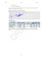
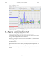
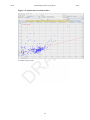
9.4. Spatial autocorrelation chart
The spatial autocorrelation chart is only available when the expert mode is enabled.
For each territorial unit of the study area, this chart crosses the values of the spatial deviation on absissa
axis with the values of the territorial deviation on ordinates axis.
This chart is very interesting for expert users as it reveals spatial dependancy, e.g. spatial organization
of a phenomena.
More empirically, the chart can also be used to examine the situation of outliers and exceptional units
out of the cloud of points.
The compute of this chart is based on a Moran's coefficient of spatial autocorrelation variant. The
regression line is drawn in red on the chart, its equation, computed by the least squares method, is
displayed on the left corner of the frame, as shown on Figure 9.5.
Each unit is drawn as a blue square, its name is displayed in a tooltip when the mouse comes over
the square.
43
Draft
Standard HyperAtlas Expert Mode
Figure 9.5. Spatial autocorrelation chart
Available in expert mode.
44
Draft
Draft
Draft
Part III. HyperAdmin
Draft
Draft
Table of Contents
10. Standard HyperAdmin Overview ..............................................................................
11. Geometry input ......................................................................................................
11.1. The MID file ..............................................................................................
11.2. The MIF file ...............................................................................................
11.3. Layer of main cities .....................................................................................
12. Structure/Contiguity input ........................................................................................
12.1. Structure input ............................................................................................
12.2. Contiguity input (optional) ............................................................................
13. Stocks input ..........................................................................................................
13.1. HyperAdmin input data file format .................................................................
13.1.1. About ..............................................................................................
13.1.2. Data ................................................................................................
13.1.3. Default ............................................................................................
13.1.4. Label ..............................................................................................
13.1.5. Metadata ..........................................................................................
13.1.6. Provider ..........................................................................................
13.1.7. RatioStock .......................................................................................
13.1.8. StockInfo .........................................................................................
14. Standard HyperAdmin build .....................................................................................
46
47
48
48
49
52
54
54
58
64
64
64
64
65
65
66
66
66
67
69
Draft
Draft
Chapter 10. Standard HyperAdmin
Overview
In order to perform Multiscalar Territorial Analysis with Standard HyperAtlas, the datasets provided by geographers are serialized in a convenient format into a binary file named with the .hyp extension. As a convention, a Standard HyperAtlas dataset input file is called an hyp file (example:
demography.hyp).
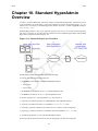
Standard HyperAdmin is the tool to generate hyp files from your a set of input well-formed files.
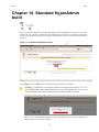
The steps to generate an hyp file and the workflow between Standard HyperAdmin and Standard
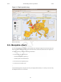
HyperAtlas is summarized in the Figure 10.1.
Figure 10.1. Standard HyperCarte Workflow
Standard HyperAdmin and Standard HyperAtlas data flow.
To sum up, the main expected input files are:
• the geometry of the dataset, in MapInfo MIF/MID formats:
• the MIF file
• the MID file
• the structure of the dataset, as an xls (Excel/OpenOffice) file
• the stocks of the dataset, as an xls (Excel/OpenOffice) file
As shown on Figure 10.1, creating a dataset hyp file consists in:
1. preparing your dataset geometry as a MIF/MID files pair (MapInfo format);
2. preparing your dataset structure as a speadsheet structure.xls file;
3. optionally, preparing a distance-time matrix as an xlsfile for custom contiguities;
4. preparing your dataset stocks as a spreadsheet (Excel/OpenOffice) data.xls file;
5. generating the dataset hyp file with Standard HyperAdmin.
Following chapters describe each above step for integrating your data into an hyp file.
47
Draft
Draft
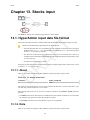
Chapter 11. Geometry input
This section describes the expected geometry input for Standard HyperAdmin.
The maps are computed using the geometric information from the lowest level of territorial
units, then aggregating this information to build the upper levels. So, the user must provide
data without any hole, and territorial units at lowest level must be contiguous.
Expected geographical information must be provided by the user in the MIF/MID format
(MapInfo format). For more information on this software and its format, please consult http://
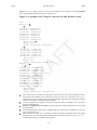
www.pbmapinfo.eu/ (last visit: 13rd may 2010).
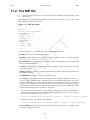
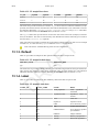
11.1. The MID file
The MID file must be made of only one column where territorial units identifiers are listed, one per
line, without any doublon. Example:
"AT111"
"AT112"
"AT125"
"AT126"
"AT127"
"AT13"
"AT211"
The given order of TU identifiers in the MID file must match the order of provided regions in
the MIF file, see Data section of the MIF file [50]
Based on a naming convention of the identifiers for these territorial units, following exceptions are
handled by HyperAtlas for particular display options. Please take into account the following exceptions
when designing your dataset:
• FR, ES, PT, MT is the list of units identifiers for countries that own overseas units: France (Martinique, ...), Spain (Canarias, ...) and Portugal (Madeire). For example for European datasets, In
HyperAtlas, the islands will be drawn in squares over the Russia.
• SUR and BRA (Surinam and Brazil) are examples of units identifiers that are treated differently
when drawing them on the maps by HyperAtlas.
• Integer identifiers from 0 to 9 correspond to squares that must be drawn on the map, they are used
for overseas in Europe dataset.
• A territorial unit with the identifier no data will be painted in white on the maps that are drawn by
HyperAtlas. This exception is used for North Cyprus in Europe datasets.
• The chypre identifier is used to handle the particular case of the display of Cyprus island in the
ESPON datasets.
48
Draft
Geometry input
Draft
11.2. The MIF file
The information in this section is essentially based on the MapInfo Data Interchange Format
document [2].
Geographical units are described in an ASCII file by their X and Y coordinates. The .MIF file is made
of an header section then a data section.
Figure 11.1. MIF file header
VERSION n
Charset ”characterSetName”
[ DELIMITER ”<c>” ]
[ UNIQUE n,n.. ]
[ INDEX
n,n.. ]
[ COORDSYS...]
[ TRANSFORM...]
COLUMNS n
<name> <type>
<name> <type>
etc.
As shown on Figure 11.1, the header can contain the following information:
• VERSION: the version of the MapInfo software;
• CHARSET clause specifies which character set was used to create text in the table (examples:
WindowsLatin1, MacRoman or Neutral;
• DELIMITER shows the character that is used to separate columns values (if not specified, tabulation is the default delimiter);
• UNIQUE parameter must be a number that refers to a database column, this parameter is used to
create related tables;
• INDEX parameter (a number or a comma-separated list of numbers) that shows the number(s) of
the indexed column(s);
• the COORDSYS parameter sets the used coordinate system.
This parameter is essential, in particular to compute the scale of the map. By default (when no COORDSYS clause is specified) data is assumed to be stored in longitude/latitude forms. All coordinates are stored with respect to the northeast quadrant. The coordinates for points in the West of
Greenwich have a negative X while coordinates for points in the East of Greenwich have a positive
X. Coordinates for points in the Northern hemisphere have a positive Y while coordinates for points
in the Southern hemisphere have a negative Y. Examples:
• The following example represents a map of Europe centered on 50°N 15°E with a Lamber Azimutal projection that can be associated to the following bounds pair: (Xmin, Ymin) (Xmax, Ymax).
The "m" option stands for "meters" as the unit:
CoordSys NonEarth Units "m" Bounds (-2217175, -1723801) (1783333, 2518193)
• Another setting for a map of Rhône-Alpes may be:
CoordSys NonEarth Units "m" Bounds (691594, 1893320) (993392, 2185448)
• TRANSFORM parameter can be used to convert coordinates which are given in a different quadrant than the default northeast one.
49
Draft
Geometry input
Draft
• COLUMNS parameter describes the data in the table of the associated MID file. The n parameter
specifies the number of columns. Example:
Columns 1
unit Char(100)
specifies one column named unit, each value will be made of characters string type whose length
is not longer than 100.
HyperAdmin is quite sensible on the format of the header of the MIF file (one information by
line). Here are some examples of the expected formats for the header of the more frequently
recent and used MIF files:
• European datasets (used for ESPON HyperAdmin maps with the EPSG 3035 Coordinates
system and projection):
Version 300
Charset "Neutral"
Delimiter ","
CoordSys NonEarth Units "m" Bounds (2600301.93555, 1249109.375) (6593124.
Columns 1
ID Char(50)
Data
(...)
• EUROMED dataset:
Version 300
Charset "WindowsLatin1"
Delimiter ","
CoordSys NonEarth Units "m" Bounds (-4487557.26071, -3722255.38453) (4487
Columns 1
ID Char(10)
Data
(...)
• Metroborder dataset:
VERSION 300
Charset "WindowsLatin1"
DELIMITER ";"
COORDSYS NonEarth Units "m" Bounds (-743051.308162917,-145654.445989655)
COLUMNS 1
SHN Char(14)
DATA
(...)
The DATA keyword specifies both the end of the header of the MIF file and the start of the enumeration of outlines.
If the MapInfo MIF file may set different types of graphical primitives (point, line, polyline, etc.),
the HyperAdmin software only expects the polygon type in order to describe the outlines of territorial
units. Eeach TU whose identifier is given in the MID file (see Section 11.1) must be associated to
a new entry in the MIF file under the data section, IN THE SAME ORDER, as a Region entry. In
50
Draft
Geometry input
Draft
MapInfo, a Region object consists of one or more polygons. Let us describe an expected Region
entry using the definition example shown on Figure 11.2.
Figure 11.2. Example of two "Region" entries in the MIF file Data section
Data
Region 2
7
108071.871 -293320.749
96339.456 -282096.297
102833.097 -261179.193
106485.534 -258631.56
123883.98 -262981.491
122621.886 -282959.13
108071.871 -293320.749
Pen (1,2,0)
Brush (0,1)
Center 110111.718 -275976.153
5
-407753.01 -311500.065
-417000.993 -311417.496
-411718.965 -289228.641
-406514.985 -302217.573
-407753.01 -311500.065
Pen (1,2,0)
Brush (0,1)
Center -411757.989 -300364.353
Region 1
11
2186917.593 -1518464.703
2186829.009 -1692861.786
2129979.423 -1729141.275
1933829.46 -1729141.275
1928265.747 -1699690.677
1922979.324 -1671615.192
1928499.903 -1666190.274
1941660.768 -1656068.01
2005909.794 -1679948.187
2047505.1 -1676110.68
2186917.593 -1518464.703
Pen (1,2,0)
Brush (0,1)
Center 2140313.457 -1623802.989
Start of the entry for the first territorial unit in our data section. This region definition will be
associated to the identifier on the firts entry of the MID file. The 2 parameter near Region
shows that this region is made of two polyogons (example, France may be considered as a region
made of two polygons: metropol and Corse island).
The first polygon of this region is set with seven points whose coordinates in X Y forms are
given on following lines.
Pen(a, b, c), Brush(a, b) and Center x y specifications are optional and they will not be read
by HyperAdmin.
The second polygon of this region is defined with five points whose coordinates are given on
the five following lines.
Here is the start of a new Region definition. As the second entry of the data section, this region
definition will be associated to the identifier on the second line of the MID file. Region 1
indicates that this region is made of one polygon.
51
Draft
Geometry input
Draft
This line shows the number of points that compose the polygon: 11 points, whose coordinates
are successively given on 11 folloging lines.
11.3. Layer of main cities
HyperAtlas can handle additional layers of information that can be displayed over the maps. Currently
(May 2011), only a layer showing the main cities has been tested and can currently be supported.
The expected format for this "cities" layer incorporation into the dataset to be built is a .csv file. This
file is only composed of three fields, these fields are separated by a comma character:
• the name of the city
• the X coodinate of this city, based on the MIF/MID projection and coordinates system
• the Y coodinate of this city, based on the MIF/MID projection and coordinates system
The following listing provides an example of the main cities layer definition csv file that has been
used for European datasets (EPSG 3035):
Vilnius,5295673.924,3612560.328
Minsk,5460580.445,3560616.774
Dublin,3253284.971,3480193.09
Berlin,4547186.818,3272495.918
Amsterdam,3975886.565,3263689.867
Warszawa,5068508.328,3293815.926
London,3620060.313,3202333.12
Bruxelles/Brussel,3927032.583,3095975.903
Kyiv,5751996.553,3239855.146
Praha,4639737.703,3008973.669
Paris,3769691.587,2891825.057
Wien,4790135.661,2807741.98
Budapest,5003603.404,2753261.228
Bern,4128054.027,2651781.399
Beograd,5142183.84,2467117.484
Bucuresti,5593724.067,2506886.924
Sofiya,5408445.047,2274434.026
Tirana,5143864.946,2078891.927
Madrid,3164690.758,2032301.915
Ankara,6248076.399,2163898.451
Helsinki,5144699.201,4208069.911
Zagreb,4784474.809,2540154.601
Nicosia,6434072.209,1668719.112
Luxembourg,4054388.133,2965578.225
Bratislava,4859375.987,2822228.019
Tallinn,5154761.636,4105585.175
Sarajevo,4997878.051,2344715.534
Skopje,5274194.7,2172377.111
Athina,5518075.047,1777730.958
Kishinev,5733746.751,2835203.886
Copenhagen,4481880.455,3626362.309
Lisboa,2671218.026,1947183.08
Oslo,4362362.69,4091266.484
Reykjavik,2843090.801,4908517.82
Riga,5170116.607,3836021.74
Roma,4531433.066,2089563.772
Stockholm,4781578.636,4041161.089
52
Draft
Geometry input
Valletta,4737055.11,1442089.281
Ljubljana,4670851.053,2559186.916
El-Jazair,3696198.974,1536632.051
Tounis,4344016.475,1511814.733
Podgorica,5085720.438,2197200.507
Vaduz,4287807.431,2668956.206
53
Draft
Draft
Draft
Chapter 12. Structure/Contiguity input
The Section 12.1 presents the expectations of the Standard HyperAdmin about the structure input file,
e.g. the information about the territorial units hierarchy and their relationships.
The Section 12.2 presents the optional steps that consists in creating a distance-time contiguity matrix
input data for custom neighbourhood definitions (example: distance time, 2 hours by car, etc.).
12.1. Structure input
In the the input structure.xls Excel file, ten sheets must mandatory be provided in a unique
.xls file.
Optionnally, complex contiguities must be defined as a set of seven sheets in an unique other xls file.
Thus the input data may be composed of:
• some_structure.xls: to describe the structure;
• some_contiguity.xls: to optionally describe the contiguities (see Section 12.2).
Table 12.1 provides the list of these sheets names and a short description for each of them, as they
are expected in the structure input definition. The expected columns and an example for each of
them is described below this table.
The names of sheets is case-unsensitive. For example, the mandatory UnitArea.txt file
can be named unitarea.txt or UNITAREA.txt. Suffixes and prefixes around the file
basename are also possible while choosing the plain text option: thus, my_UnitArea.txt
will be considered as a UnitArea.txt file, e.g. the input file that contains the information
about the relationships between areas and territorial units.
54
Draft
Structure/Contiguity input
Draft
Table 12.1. Overview of expected sheets for data structure input
Excel Sheet Name
Description
unit
Identifiers for the set of territorial units. See
Content of unit.
Area
Identifiers for the set of study areas. See Content
of area.
Zoning
Identifiers for the set of meshes. See Content of
zoning.
UnitSup
Hierarchy between units: an UTSup_ID parent unit owns at least one child UT_ID unit. See
Content of unitsup.
UnitArea
An UT belongs to one or several study areas.
See Content of unitarea.
UnitZoning
An UT belongs to one or several meshes. See
Content of unitzoning.
language
Provides a human readable name for used languages codes. See Content of language.
UnitLanguage
Names of UT in different languages. A translation may be missing. See Content of unitlanguage.
AreaLanguage
Names of the study areas in different languages.
A translation may be missing. See Content of
arealanguage.
ZoningLanguage
Names of the meshes in different languages. A
translation may be missing. See Content of zoninglanguage.
Expected content for each of these sheets is following:
Unit
This file/sheet must contain one column whose header cell must be UT_ID.
Example:
Table 12.2. Sample input Unit sheet
UT_ID
AT11
AT12
AT13
AT21
etc...
Area
This file/sheet must contain one column whose header cell must be Area_ID.
Example:
55
Draft
Structure/Contiguity input
Draft
Table 12.3. Sample input Area sheet
Area_ID
UE15
UE25
PECO
Arc_Atlantique
Nouveaux_UE
UE27
UE29
Zoning
This file/sheet must contain one column whose header cell must be
Zoning_ID. An additional column named Rank may order given zonings.
Example:
Table 12.4. Sample input Zoning sheet
UnitSup
Zoning_ID
Rank
Nuts_0
1
Nuts_1
2
Nuts_2
3
Nuts_3
5
Nuts_2_3
4
This file/sheet must contain two columns whose header cells must be named
UTSup_ID and UT_ID. Example:
Table 12.5. Sample input UnitSup sheet
UnitArea
UT_ID
UTSup_ID
AT1
AT
AT2
AT
AT3
AT
BE1
BE
BE2
BE
This file/sheet must contain two columns whose header cells must be named
UT_ID and Area_ID. Example:
Table 12.6. Sample input UnitArea sheet
UT_ID
Area_ID
AT
UE15
BE
UE15
DE
UE15
DK
UE15
ES
UE15
56
Draft
Structure/Contiguity input
UnitZoning
Draft
This file/sheet must contain two columns whose header cells must be UT_ID
and Zoning_ID. Example:
Table 12.7. Sample input UnitZoning sheet
Language
UT_ID
Zoning_ID
AT
Nuts_0
BE
Nuts_0
BG
Nuts_0
CH
Nuts_0
This file/sheet must contain two columns whose header cell are
Language_ID and Language_NAME. Example:
Table 12.8. Sample input Language sheet
UnitLanguage
Language_ID
Language_NAME
DE
allemand
CS
tchèque
DA
danois
ET
estonien
EN
anglais
ES
espagnol
This file/sheet must contain three columns whose header cells must be UT_ID,
UT_NAME and Language_ID. Example:
Table 12.9. Sample input UnitLanguage sheet
AreaLanguage
UT_ID
Language_ID
UT_NAME
AT11
DE
BURGENLAND
AT34
DE
VORARLBERG
BE24
NL
VLAAMS BRABANT
BE25
NL
WESTVLAANDEREN
BE31
FR
BRABANT WALLON
BE32
FR
HAINAUT
This file/sheet must contain three columns whose header cells must be
Area_ID, Language_ID and Area_NAME. Example:
Table 12.10. Sample input AreaLanguage sheet
Area_ID
Language_ID
Area_NAME
UE15
FR
Union européenne des
15
UE25
FR
Union européenne des
25
PECO
FR
Pays d'Europe Centrale
et Orientale
57
Draft
Structure/Contiguity input
ZoningLanguage
Draft
This file/sheet must contain three columns whose header cells must be
zoning_ID, Language_ID and zoning_NAME. Example:
Table 12.11. Sample input ZoningLanguage sheet
Zoning_ID
Language_ID
Zoning_NAME
Nuts_0
FR
Nomenclature des unités
territoriales de niveau 0
Nuts_1
FR
Nomenclature des unités
territoriales de niveau 1
Nuts_2
FR
Nomenclature des unités
territoriales de niveau 2
Nuts_3
FR
Nomenclature des unités
territoriales de niveau 3
Nuts_2_3
FR
Nomenclature des unités
territoriales de niveau
2-3
12.2. Contiguity input (optional)
This section presents the optional contiguity definition input data file.
Table 12.12. Overview of expected sheets for contiguity input
Excel Sheet Name
Description
Contiguity
List of identifiers for contiguities.
ContiguityLanguage
Names of the contiguities in different languages.
A translation may be missing. See Content of
contiguitylanguage.
Neighbourhood
Unique code for a neighbourhood that is associated to a contiguity, a threshold and a comparator. The comparator shows if two UT are neighbours or not. See Content of neighbourhood.
Neighbourhood
Names of neighbourhoods for each language.
A translation may be missing. See Content of
neighbourhoodlanguage.
ContiguityZoning
A distance matrix is available for one or several
meshes. See Content of ContiguityZoning.
ContiguityArea
A distance matrix is available for one or several
study areas. See Content of ContiguityArea.
UnitContiguityi
Each line provides the code of two UT,
following columns show the distance for
Contiguity_IDi, the header cell of each contiguity column providing the identifier of this
contiguity. See Content of UnitContiguity.
Following listing provides an example for each expected sheet describing a contiguity definition:
58
Draft
Structure/Contiguity input
Contiguity.txt / Contiguity
Draft
This sheet must contain one column whose header cell is ID.
Example: the following sample sets two possible computations
for contiguity, distance-time matrixes will be available for a car
and for a lorry.
Table 12.13. Sample input Contiguity sheet
ID
CAR
TRUCK
ContiguityLanguage.txt / ContiguityLanguage
This sheet must contain four columns whose header cells are
CONTIGUITY_ID, Language_ID (see Note about expected
languages identifiers), Contiguity_NAME (e.g. the name of
this contiguity in this locale) and Contiguity_DESC (a description of this contiguity). Example:
Table 12.14. Sample input ContiguityLanguage
sheet
Contiguity_IDLanguage_ID Contiguity_NAME
Contiguity_DESC
Neighbourhood.txt / Neighbourhood
CAR
EN
car time
Time between
units by car (in
minutes)
TRUCK
EN
truck time
Time between
units on a
truck
(minutes)
CAR
FR
temps voiture Temps entre
les unités en
voiture (minutes)
TRUCK
FR
temps camion Temps entre
les unités en
camion (minutes)
This sheet must contain four columns whose header cells are
Neighbourhood_ID (see Note about expected languages
identifiers), Contiguity_ID, Distance and Comparator. Possible values for the Comparator cells are:
• <
• <=
• ==
• >=
• >
Example:
59
Draft
Structure/Contiguity input
Draft
Table 12.15. Sample input Neighbourhood sheet
Neighbourhood_ID
Contiguity_IDdistance
comparator
CAR <= 360
TRUCK
360
CAR
360
<=
<= TRUCK
360
<=
CAR
540
<=
<= TRUCK
540
<=
CAR
180
<=
<= TRUCK
180
<=
CAR <= 540
TRUCK
540
CAR <= 180
TRUCK
180
NeighbourhoodLanguage.txt /
NeighbourhoodLanguage
This sheet must contain four columns whose header cells are
Neighbourhood_ID, Language_ID (ISO-639 language
in 2 digits, Neighbourhood_NAME (e.g the name of this
neighbourhood) and Neighbourhood_DESC (e.g. a description of this neighbourhood). In the following example, neighbourhoods are translated in english (EN) and french (FR):
60
Draft
Structure/Contiguity input
Draft
Table
12.16.
Sample
NeighbourhoodLanguage sheet
input
Neighbourhood_ID
Language_ID Neighbourhood_NAME
Neighbourhood_DESC
CAR <= 360
TRUCK
360
<= EN
CAR <= 540
TRUCK
540
ContiguityZoning.txt / ContiguityZoning
Units at less
than 6 hours
by car
6h truck
Units at less
than 6 hours
on a truck
9h car
Units at less
than 9 hours
by car
9h truck
Units at less
than 9 hours
on a truck
3h car
Units at less
than 3 hours
by car
3h truck
Units at less
than 3 hours
on a truck
6h de voiture Unités
à
moins de 6
heures
en
voiture
<= FR
6h de camion Unités
à
moins de 6
heures
en
camion
FR
<= FR
CAR <= 180
TRUCK
180
6h car
FR
CAR <= 540
TRUCK
540
EN
<= EN
CAR <= 360
TRUCK
360
EN
<= EN
CAR <= 180
TRUCK
180
EN
9h voiture
Unités
à
moins de 9
heures
en
voiture
9h de camion Unités
à
moins de 9
heures
en
camion
FR
3h de voiture Unités
à
moins de 3
heures
en
voiture
<= FR
3h de camion Unités
à
moins de 3
heures
en
voiture
This sheet must contain two columns whose header cells are
Contiguity_ID and Zoning_ID. In the following example, the distance-time by car and distance-time by lorry are
available for NUTS_2 zoning only:
61
Draft
Structure/Contiguity input
Draft
Table 12.17. Sample input ContiguityZoning
sheet
Contiguity_ID
Zoning_ID
CAR
Nuts_2
TRUCK
Nuts_2
The identifiers that are given in the Zoning_ID column must be coherent with the identifiers that have
been given in the Zoning sheet of the structure input,
see Content of zoning.
ContiguityArea.txt / ContiguityArea
This sheet must contain two columns whose header cells are
Contiguity_ID and Area_ID. In the following example, distance-time matrixes by car are available for UE15 and
UE25, distance-time matrixes by lorry are available for UE27
and UE29:
Table 12.18. Sample input ContiguityArea sheet
Contiguity_ID
Area_ID
CAR
UE15
CAR
UE25
TRUCK
UE27
TRUCK
UE29
The identifiers that are given in the Area_ID column
must be coherent with the identifiers that have been given in the Area sheet of the structure input, see Content
of area.
UnitContiguity.txt / UnitContiguityi
This sheet must contain at least three columns whose header
cells are UT_ID1, UT_ID2, then the identifier of a contiguity..
In the following example, contiguities between units are performed for CAR contiguity and TRUCK contiguity:
Table 12.19. Sample input UnitContiguity sheet
UT_ID1
UT_ID2
CAR
TRUCK
ES12
UKC1
1265.11
1820.5
ES13
UKC1
1138.85
1649.5
ES21
UKC1
1058.92
1529.9
In Excel mode, each UnitContiguity can only contain 216 rows, e.g. 65536. Several sheets can be created
to import more results: just name your sheets UnitContiguity1, UnitContiguity2, etc. Note that
only 30 UnitContiguityi sheets can be created.
Nevertheless, on considering a symetric relationship for
a distance between two units (e.g. distance between
UT1 and UT2 equals the distance between UT2 and
UT1), the number of needed rows can quasi be reduced
by half. Thus, the number S of needed sheets for n units
62
Draft
Structure/Contiguity input
Draft
can be found by executing the formula which is shown
on Figure 12.1:
Figure 12.1. Number S of needed sheets for
n units
S is the number of needed sheets, n is the number of
units. On the numerator, "1 +" stands for the header
row that must be included on each sheet.
Note that contiguities are not aggregable: a distance
matrix is set for a given level of mesh. For its upper
level, the associated distance matrix must also be given. Table 12.20 provides an example of the number of
needed sheets for different levels with several numbers
of units.
Table 12.20. Example of needed sheets
number
Mesh
Number of UT Number of
(n)
sheets (S)
NUTS_0
29
1
NUTS_1
92
1
NUTS_2
280
2
NUTS_2_3
727
5
NUTS_3
1329
14
Total 23
63
Draft
Draft
Chapter 13. Stocks input
The stock file mainly aims at describing the statistics of the dataset.
13.1. HyperAdmin input data file format
This section describes the stocks (statistical data) file that Standard HyperAdmin expects as input.
Please note the following requirements for the input data file:
• the input data file must be a spreadsheet xls file (editable by Microsoft Excel and Open
Office) named "*data*.xls": the filename must include the "data" characters sequence
and the .xls extension is required.
• the values of stocks must be provided for the lowest level of territorial units. This list is
available in the example data template that depends on the selected structure/geometry model at previous step.
• all values for all units must be filled;
Following sections describe the expected format (sheets, columns and possible values) for the version
2 of this data.xls "stocks" file.
13.1.1. About
Table 13.1 provides an example for this mandatory sheet in the data v2 input xls file.
Table 13.1. V2 sample About sheet
VERSION
TIME_ENABLED
2
TRUE
This sheet aims at identifying the version of the format of this data file. Currently (2010-2011), only
the value 2 is possible for the VERSION column.
The expected value for the TIME_ENABLED column is a boolean: only TRUE or FALSE values are
possible:
• The TRUE value shows that values are available for the sames labels of indicators at several dates:
for example, the population in 2000, the population in 2002.
• The FALSE value shows that each indicator is given for a single date.
13.1.2. Data
Table 13.2 provides an example for this mandatory sheet in the data v2 input xls file.
64
Draft
Stocks input
Draft
Table 13.2. V2 sample Data sheet
UT_ID
pop2000
pop2002
area2000
gdp2000
gdp2002
AT111
1
15
2
7
10
AT112
3
16
4
8
11
AT113
5
17
6
9
12
This sheet must provide at least three columns: UT_ID then at least two indicators identifiers (in HyperAtlas, there must be at least one numerator stock and one denominator stock). The Table 13.2 shows
five indicators identifiers: pop2000, pop2002, area2000, gdp2000 and gdp2002. These identifiers must be described in the StockInfo sheet (see Section 13.1.8).
The UT_ID column must provide the list of territorial units at the lowest rank (example, at NUTS 3
level) of the dataset. The units are referenced by their identifiers that must match the given values in
the associated structure.xls input file.
Then, each other cell provides a value for the given indicator column at the given unit row. For example
in Table 13.2, 17 is the value for pop2002 indicator in AT113 territorial unit.
Each cell must be valuated. Missing values are not accepted here.
13.1.3. Default
Table 13.3 provides an example for this optional sheet in the data v2 input xls file.
Table 13.3. V2 sample Default sheet
DEFAULT_NUM
DEFAULT_DEN
pop
area
This sheet aims at providing a default indicator to be selected in HyperAtlas at startup for the denominator and for the numerator combo boxes. Expected values for both columns are valid indicators
identifiers that must match two of those defined in the StockInfo sheet (see Section 13.1.8).
13.1.4. Label
Table 13.4 provides an example for this mandatory sheet in the data v2 input xls file.
Table 13.4. V2 sample Label sheet
LABEL_ID
LANG_CODE
NAME
DESC
1
EN
Total population
Total population
thousands
in
1
FR
Population totale
Population
milliers
en
2
EN
Area
Total area
2
FR
Superficie
Superficie totale
3
EN
GDP
Gross domestic product
3
FR
PIB
Produit intérieur brut
4
EN
GDP/Inhabitant
Gross domestic product
per inhabitant
4
FR
PIB/Hab
PIB par habitant
5
EN
Density
Density of population
5
FR
Densité
Densité de population
65
totale
Draft
Stocks input
Draft
This sheet aims at providing the internationalized names and descriptions for the indicators and predefined ratios. The LABEL_ID and LANG_CODE provides indexes for this table: for a given label
identifier there may be several available translations. Thus, the LABEL_ID = 1 is available in english (LANG_CODE = EN) and french (LANG_CODE = FR) languages. In the StockInfo sheet,
each indicator reference a label identifier. As several indicators may be similarly named and described
(when an indicator is valuated for several dates), these labels have been exported here.
The language identifier code must be a valid ISO Language Code. These codes are the lower-case, two-letter codes as defined by ISO-639. Nevertheless, the parser supports upper-cases.
You can find a full list of these codes at a number of sites, such as: http://www.ics.uci.edu/
pub/ietf/http/related/iso639.txt (2011-03-16).
Note that values in the LABEL_ID column may be referenced from the StockInfo sheet (see Section 13.1.8) and from the RatioStock sheet (see Section 13.1.7).
13.1.5. Metadata
Table 13.5 provides an example for this optional sheet in the data v2 input xls file.
Table 13.5. V2 sample Metadata sheet
UT_ID
STOCK_ID
PROVIDER_ID
AT111
pop2000
1
AT112
pop2000
2
area
2
pop2002
1
This draft sheet aims at providing some basic metadata information for an indicator relatively or not
to a territorial unit. Currently, only the source of data may be given as metadata.
For example in Table 13.5, the values of the pop2000 indicator identifier were retrieved from different sources for regions AT111 and AT112. On the contrary, all values for the area indicator,
whatever the unit is, were provided by the same source. Idem for the pop2002 indicator.
The values in the PROVIDER_ID column must match the identifiers that are given in the Provider
sheet (see Table 13.6). Likewise, the values in the STOCK_ID column must match the identifiers that
are defined in the StockInfo sheet (see Table 13.8).
13.1.6. Provider
Table 13.6 provides an example for this optional sheet in the data v2 input xls file.
Table 13.6. V2 sample Provider sheet
PROVIDER_ID
NAME
CONTACT
URL
1
Eurostat
[email protected]
http://www.eurostat.eu
2
INSEE
[email protected]
http://www.insee.fr
This sheet aims at providing the list of data providers. Their different ids are referenced from the
Metadata sheet.
13.1.7. RatioStock
Table 13.7 provides an example for this optional sheet in the data v2 input xls file.
66
Draft
Stocks input
Draft
Table 13.7. V2 sample RatioStock sheet
RATIO_ID
LABEL_ID
NUM_ID
DEN_ID
VALIDITY_START
VALIDITY_END
1
4
gdp2000
pop2000
2000
2000
2
4
gdp2002
pop2002
2002
2002
3
5
pop2000
area2000
2000
2000
4
5
pop2002
area2000
2002
2002
This sheet aims at defining relevant ratios for the HyperAtlas "ratio" combo box parameter. Table 13.7
shows the example of two such predefined ratios, each of them for two different dates:
• the GDP/Inhabitant:
• in 2000 (second line)
• in 2002 (third line)
• The density of population:
• in 2000 (fourth line)
• in 2002 (fifth line)
Each value in the RATIO_ID column must be unique. Doublons will overwrite the previous found
value.
Note that the LABEL_ID references the sames labels for the given pairs of numerator/denominator at
different dates (4 for lines 2 and 3, 5 for lines 4 and 5). These labels identifiers must be set in theLabel
sheet (see Section 13.1.4).
The values in the NUM_ID column and the values in the DEN_ID column must match the identifiers
of indicators that are defined in the StockInfo sheet (see Section 13.1.8).
The values in the VALIDITY_START column will only be considered if the value of the
TIME_ENABLED column in the About sheet is TRUE (see Section 13.1.1). Then, one relevant ratio
can be chosen in HyperAtlas for different dates. Identically for the values in the VALIDITY_END
column. Though VALIDITY_START and VALIDITY_END columns are designed to handle time intervals, setting the same value in both columns makes the ratio associated to a timestamp.
The expected format for both valididy start/end date fields is currently a year in the yyyy
pattern. An input like 2010-12-31 is possible but this version of the application will only
take into account the year, that is to say 2010 for this example.
13.1.8. StockInfo
Table 13.8 provides an example for this mandatory sheet in the data v2 input xls file.
Table 13.8. V2 sample StockInfo sheet
STOCK_ID
LABEL_ID
MEASURE_UNIT
VALIDITY_START
VALIDITY_END
VISIBLE_FLAG
pop2000
1
*1000
2000
2000
TRUE
pop2002
1
*1000
2002
2002
TRUE
area2000
2
km2
2000
2000
TRUE
gdp2000
3
euros
2000
2000
TRUE
gdp2002
3
euros
2002
2002
TRUE
67
Draft
Stocks input
Draft
This sheet mainly aims at providing the identifiers of the indicators of the dataset. Here are a short
description for each column of this sheet:
• STOCK_ID: each value in this column must be unique. Any doublon will overwrite the previous
found identical value. This column lists the identifiers of the indicators that are referenced in the
other sheets. Note that several indicators may be associated to the same label (lines 2 and 3 for
example), though they exist to distinguish the values of the population in 2000 and 2002.
• LABEL_ID: each value in this column must reference an identifier defined in the Label sheet (see
Section 13.1.4).
• MEASURE_UNIT: simply provides the unit of measure for this indicator.
• VALIDITY_START: shows the start date of validity for this indicator. This field will only be
considerated if the value of the TIME_ENABLED column in the About sheet is TRUE (see Section 13.1.1 and Important note about expected date format).
• VALIDITY_END: shows the end date of validity for this indicator. VALIDITY_START and
VALIDITY_END fields are able to manage time intervals, but they can be used to associate a timestamp to the current stock: just write the same value in both cells (please see Important note about
expected date format).
• VISIBLE: this field acts like a flag, a boolean is expected for the values of this column. A TRUE
value shows that this indicator will be available in the numerator and in the denominator combo
boxes of HyperAtlas parameters panel. A FALSE value may be usefull to define relevant ratios
whose indicators have no reason to be available in the numerator and denominator combo boxes.
For example, the life expectancy pre-defined ratio considers indicators that have no sense out of
this compute.
68
Draft
Draft
Chapter 14. Standard HyperAdmin
build
Once the user has submitted a well-formed spreadhseet file including his/her stocks for the chosen
geometry at step 1, he/she is redirected to the "Build" page, see Figure 14.1. He/she is invited here
to enter a name and a description for the dataset hyp file he/she is about to generate. These fields are
mandatory.
Figure 14.1. Dataset information form
The stock data file is well-formed. Enter a name and a description for the dataset.
Depending on the wideness of the dataset (number of stocks/geometries/zonings, etc.), this
step may take a while. While building the dataset, a progress bar appears after a few seconds
in the foreground of the window, the backgound page functionnalities are disabed:
Please do not click the submit button as long as the page has not completly reloaded and
displayed a success or failure message.
69
Draft
Standard HyperAdmin build
Draft
If the generation of the hyp file is successfull, the user is redirected to a success page where he/she
can download his/her new dataset. Else, an error message is displayed on this "build" page.
In case of success (Figure 14.2), the ouput build logs are summarized and displayed on the page. In
order to avoid overwriting, note that the generated hyp filename follows a date pattern: yyyyMMddhhmmss (year month date hour minutes seconds). On clicking the link showing the name of the
generated dataset, the user is invited to save the file to his/her disk, of course he/she can rename the
hyp file at his/her convenience.
The use of Microsoft Internet Explorer browser may disturb users when clicking the link by
opening an ununderstanble page showing the content of the binary hyp file: to download the
generated dataset, right-click the link and choose "Save target as" in the displayed contextual
menu.
Figure 14.2. Successfull build
Clicking the link at the bottom of the page invites the user to download his/her generated dataset as
an hyp file.
70
Draft
Draft
Appendix A. Annex: when things go
wrong...
This section deals with the problems that may occurre when using the described tools in this document.
Below Known bugs section proposes a non-exhaustive list of problems that can be worked around
when using the Standard HyperAtlas software.
Like most of Java applets, the Standard HyperAtlas software displays logs messages to the "Java
Console". This window is not enabled by default on most of standard browsers. If Standard HyperAtlas
does not behave as expected and described in this user's manual, first enable this Java Console. Note
that the display of the Java console depends on your operating system and on your Web browser.
Please consult the following links (last visit: 20101228):
• Windows users: How do I enable and view the Java Console? [http://www.java.com/en/download/help/javaconsole.xml];
• Mac OS X users: Java Frequently Asked Questions [http://developer.apple.com/java/faq/]
• RedHat and Suse Linux users: How do I enable and view the Java Console for Linux? [http://
www.java.com/en/download/help/5000021200.xml].
For problems that might happen when browsing the pages of the Standard HyperCarte Web Application, a custom page has been created in order to trace some information. Please copy paste the page
and send it to the administrator with as many details on how it happened as possible.
In order to improve the application, thanks in advance for your cooperation, please report bugs!
As far as possible, complete your message with eventual output logs, information about your
environment, the version of the application, etc.
For any comment question or suggestion, please contact the manager.
A.1. Known bugs
A.1.1. HyperAtlas is frozen
Standard HyperAtlas sometimes seems frozen as nothing happens when changing a parameter. Most
of the time, your java console will display the log message shown on Figure A.1.
A simple action allows to workaround this bug: simply resize your window!
Figure A.1. Java console: stroke shape error
Displayed log message when the maps of HyperAtlas seem frozen.
71
Draft
Annex: when things go wrong...
Draft
A.1.2. Deviations maps update
The deviations maps may sometimes appear "all in grey"... Just click the deviation context combo box
in the parameters panel in order that HyperAtlas takes into account the changes of references.
A.1.3. Multiple boxes appear
After several analysis with several datasets, multiple messages boxes may appear. As a Java Applet
is loaded in memory for a whole browser session, multiple instances may cause this problem.
The simplest thing to workaround this disturbing behaviour is to close your browser, then restart it.
This bug should be fixed in a next iteration.
72
Draft
Draft
Appendix B. Annex: acronyms
Find here an alphabetical arrangement of most often used acronyms in this document:
• DBMS: DataBase Management System.
• ESPON: European Observation Network for Territorial Development and Cohesion [1].
• GDP: Gross Domestic Product.
• HTML: HyperText Markup Language.
• JRE: Java Runtime Environment.
• MTA: Multiscalar Territorial Analysis.
• NUTS: Nomenclature of territorial units for statistics (see also a definition of NUTS in the glossary).
• XML: Extensible Markup Language.
73
Draft
Draft
Appendix C. Annex: glossary
Some definitions
Deviation
The relative deviation of a given region (i) to a context is defined
by equation Figure C.1. The relative deviation depends on the
chosen context (general, medium or local), it shows the gap between the value of the unit and the average value of the context.
The deviation is expressed in a percentage of the context average
value (100 is the pivot).
74
Draft
Annex: glossary
Draft
Figure C.1. Mathematical formula of the relative
deviation
This figure shows a general formula to compute the relative deviation RD of a territorial unit i for the chosen context Context.
Needed variables are:
• Numx is the value of the indicator chosen as the Numerator parameter for the territorial unit x.
• Denx is the value of the indicator chosen as the Denominator
parameter for the territorial unit x.
• Cij is a boolean whose value depends on the chosen context:
• General context: Cij=1 if the current territorial unit j is included in the reference area, Cij=0 in other cases. For example, if the reference area is EU-15, Cij takes the value 1 for
regions of EU-15 and the value 0 for regions of the candidate
countries.
• Territorial context: Cij shows if two regions i and j belong
or not to the same area. In the case when the medium context
considers the state level, Cij takes the value 1 for regions belonging to the same state and the value 0 for regions belonging to different states.
• Spatial context: Cij shows the potential level of local interactions between two regions i and j. The local interaction may
be for example defined by a boolean variable which takes the
value 1 for contiguous regions and the value 0 for non-contiguous regions. Currently, we have decided that a region is
not neighbour to itself (Locii=0) but it is possible to choose
the solution where a region is part of its own neighbourhood
(Locii=1). Many alternative solutions are possible according
to the definition of the neighbourhood criterion (kilometres
time, cost, length of common boundary, ...) and to the measure of the potential level of interaction. This parameter may
not be a boolean but a continuous probabilistic function between 0 and 1.
See Also General deviation, Spatial deviation, Territorial deviation.
Elementary unit
The set of elementary units compose (cover) the whole area, and
constitute the elementary zoning.
See Also Elementary zoning.
Elementary zoning
Smallest division of the studied area. Each unit of this zoning is
called elementary unit.
See Also Elementary unit.
75
Draft
Annex: glossary
Draft
General deviation
Deviation when the context of reference is the general area. The
reference can be an available study area or a any value chosen by
the user.
See Also Deviation.
Spatial deviation
Deviation when the context of an unit is defined by the set of units
that belongs to its neighbourhood (for instance adjacent units),
contiguous regions by default.
See Also Deviation.
Territorial deviation
Deviation when the context is defined by a territorial unit that belongs to a chosen higher zoning level which contains the considered unit.
See Also Deviation.
NUTS (Nomenclature of territorial units for statistics)
Established by EUROSTAT for over 30 years, NUTS is a territorial subdivision system used in Europe "in order to provide a
single uniform breakdown of territorial units for the production
of regional statistics in the European Union" [1]. The NUTS zoning nomenclature for Europe organizes all units in a hierarchy of
levels:
• NUTS 0 groups administrative units at country level : France,
Germany, Spain, Italy, etc.
• NUTS 1 groups administrative units at great region level : ILE
DE FRANCE, BASSIN PARISIEN, EST, CENTRE-EST, etc.
• NUTS 2 groups administrative units at region level (Région
in France - Länder in Germany - Comunidades autonomas in
Spain, regioni in Italy) : ILE DE FRANCE, RHONE-ALPES,
PACA, etc.
• NUTS 3 groups administrative units at departement level (Département in France - Kreise in Germany - Provincias in Spain,
Provincie in Italy): Essone, Isère, Savoie, etc.
• NUTS 4 and NUTS 5 are now deprecated levels that are respectively replaced by LAU 1 and LAU 2. LAU acronym
stands for Local Administrative Unit.
Report
HTML document that lists the set of parameters used for analysis
(study area, zoning, context for deviation, indicators for numerator and denominator) and the maps which are generated by the
application.
Stock
Social-economic count, like number of deaths on 1999 year, number of births on 1999 year, total population in thousand on 1999
year. Stocks should be valued on each elementary unit. There are
also called indicators.
Study Area
Territorial space on which we will base the analysis. It can be
Europe, Cameroun, or France by example. Only one study area
can be loaded in the same time by the application.
Ratio
A ratio between two stocks which are defined and available on
the same set of territorial units.
76
Draft
Annex: glossary
Draft
Figure C.2. Ratio
Workspace
Context of analysis and selected options in the application when
working on a study area: zoom level, map mode, etc. It can be
exported to an XML file.
77
Draft
Draft
Appendix D. Annex: references
Some usefull links
[1] ESPON Coordination Unit. ESPON. [on line]. http://www.espon.eu/ (last visit: 1.st december 2009).
[2] Pitney Bowes MapInfo. Appendix J: MapInfo Data Interchange Format. [on line]. http://
resource.mapinfo.com/static/files/document/1074660800077/interchange_file.pdf (last visit: 18.th may
2010).
78
Draft
Draft
Appendix E. HyperAtlas Application
Terms and Conditions of Use
TODO
79
Draft
Draft
Appendix F. About
This document is part of the HyperCarte Research Group projects. It has been generated at the following date, 2013-07-05 15:25:58, from the svn rev 1088 sources of the docbench project.
This document has been written by the LIG STeamer team.
For any comment question or suggestion, please please visit http://hypercarte.imag.fr or contact
Jérôme Gensel <[email protected]>.
Laboratoire LIG UMR 5217, Equipe STeamer
681 rue de la Passerelle, Domaine Universitaire
BP 72
38402 Saint Martin d'Hères Cedex
FRANCE
Tel: (+33) (0)4 76 82 72 80
Fax: (+33) (0)4 76 82 72 87
Colophon
Based on DocBook technology 1, this document is written in XML format, sources are validated with
DocBook DTD 4.5CR3, then sources are transformed to HTML and PDF formats by using DocBook
xslt 1.73.2 stylesheets. The generation of the documents is automatized thanks to the docbench
LIG STeamer project that is based on Ant 2, java 3, processors Xalan4 and FOP 5. Note that Xslt
standard stylesheets are customized in order to get a better image resolution in PDF generated output
for admonitions icons: the generated sizes of these icons were turned from 30 to 12 pt.
1
[on line] DocBook.org [http://www.docbook.org] (last visit: July 2011)
[on line] Apache Ant - Welcome. Version 1.7.1 [http://ant.apache.org] (last visit: July 2011)
3
[on line] Developer Resources For Java Technology [http://java.sun.com] (last visit: July 2011). Version 1.6.0_03-b05.
4
[on line] Xalan-Java Version 2.7.1 [http://xml.apache.org/xalan-j/] (last visit: 18 november 2009). Version 2.7.1.
5
[on line] Apache FOP [http://xmlgraphics.apache.org/fop/download.html] (last visit: July 2011). Version 0.94.
2
80
Draft
Draft
Colophon
This document was generated 2013-07-05 15:25:58 (year-month-date hour:minutes:seconds) from the svn rev
1088 of the docbench project.
Based on DocBook technology 6, this document is written in XML format, sources are validated with DocBook
DTD 4.5CR3, then sources are transformed to HTML and PDF formats by using DocBook xslt 1.73.2 stylesheets.
Documents generations were automatized with ant 7, java8, processors Xalan9 and FOP 10.
Xslt standard stylesheets are customized in order to get a better image resolution in PDF generated output
for admonitions icons: the generated sizes of these icons were turned from 30 to 12 pt.
6
[on line] DocBook.org [http://www.docbook.org] (last visit: november 2009)
[on line] Apache Ant - Welcome. Version 1.7.0. [http://ant.apache.org] (last visit: 18 november 2009)
8
[on line] Developer Resources For Java Technology [http://java.sun.com] (last visit: 18 november 2009). Version 1.6.0_03-b05.
9
[on line] Xalan-Java Version 2.7.1 [http://xml.apache.org/xalan-j/] (last visit: 18 november 2009). Version 2.7.1.
10
[on line] Apache FOP [http://xmlgraphics.apache.org/fop/download.html] (last visit: 18 november 2009). Version 0.94.
7
81