Download fulltext - DiVA Portal

Gryphon - a Module for Time Integration
of Partial Differential Equations in FEniCS
Knut Erik Skare
Master of Science in Physics and Mathematics
Submission date: June 2012
Supervisor:
Anne Kværnø, MATH
Norwegian University of Science and Technology
Department of Mathematical Sciences
Sammendrag
Denne oppgaven tar sikte på å implementere tidsintegratorer i FEniCS-rammeverket.
Mer spesifikt går oppgaven ut på å velge egnede tidsintegratorer, implementere disse og
verifisere at de virker ved å anvende dem på et utvalg relevante testproblemer. Dette
arbeidet resulterte i en modul til FEniCS som fikk navnet Gryphon. Oppgaven er delt
inn i fire deler.
Del I bygger et teoretisk rammeverk som motiverer hvorfor ESDIRK-metoder (Singly
Diagonally Implicit Runge-Kutta method with an Explicit first stage) er gode løsere for
systemer av stive ordinære differensialligninger (ODEer). Det vil også bli vist hvordan
en ESDIRK metode kan brukes til å løse tidsavhengige partielle differensialligninger
(PDEer) ved å løse det semi-diskretiserte systemet som oppnås ved å først anvende en
endelig elementmetode. Vi vil begrense oss til PDEer som enten semi-diskretiseres til et
rent ODE-system eller et differensial-algebraisk system (DAE) av indeks 1.
Del II tar for seg implementasjonen av Gryphon, med fokus på nytteverdi og kodestruktur.
Del III tar for seg numeriske eksperimenter på ESDIRK-metodene som er implementert
i Gryphon. Eksperimentene vil etablere konvergens og gi kjøretidsresultater for ulike
ESDIRK-metoder. Vi vil også se at L-stabilitet er en nyttig egenskap når en jobber med
stive ligninger, ved å sammenligne en ESDIRK metode med trapesmetoden. Det blir
også verifisert at skrittlengde-kontrollerne implementert i Gryphon oppfører seg som forventet. Som testproblemer vil vi se på varmeligningen, Fisher-Kolmogorov-ligningen,
Gray-Scott-ligningene, Fitzhugh-Nagumo-ligningene og Cahn-Hilliard-ligningen.
Del IV er en brukermanual for Gryphon hvor alle parameterne brukeren kan endre vil
bli forklart. Manualen inneholder også kode for å løse varmeligningen, Gray-Scottligningene og Cahn-Hilliard-ligningen, for å hjelpe leseren i gang med å løse egne problemer.
Abstract
This thesis aims to implement time integrators in the FEniCS framework. More specifically, the thesis focuses on selecting suitable time integrators, implement these and verify
that the implementation works by applying them to various relevant test problems. This
work resulted in a module for FEniCS, named Gryphon. The thesis is divided into four
parts.
The first part builds a theoretical framework which will motivate why singly diagonally
implicit Runge-Kutta methods with an explicit first stage (ESDIRKs) should be considered for solving stiff ordinary differential equations (ODEs). It will also be shown how
an ESDIRK method can be utilized to solve time dependent partial differential equations (PDEs) by solving the semidiscretized system arising from first applying a finite
element method. We will restrict our attention to PDEs which either give rise to a pure
ODE system or a DAE (differential-algebraic equation) system of index 1.
The second part discusses the implementation of Gryphon, focusing on why such a module is useful and how the source code is structured.
The third part is devoted to numerical experiments on the ESDIRK solvers implemented
in Gryphon. The experiments will establish convergence and give some run-time statistics for various ESDIRK schemes. We will also see that L-stability is a favorable trait
when working with stiff equations, by comparing an ESDIRK method to the trapezoidal
rule. It will also be verified that the step size selectors implemented in Gryphon behaves
as expected. As test problems we consider the heat equation, the Fisher-Kolmogorov
equation, the Gray-Scott equations, the Fitzhugh-Nagumo equations and the Cahn-Hilliard
equations.
The fourth part is a user manual for Gryphon. All the parameters which can be changed
by the user are explained. The manual also includes example code for solving the heat
equation, the Gray-Scott equations and the Cahn-Hilliard equation, to get the reader
starting on solving their own problems.
Preface
This thesis completes my master’s degree in Industrial Mathematics at the Norwegian
University of Science and Technology (NTNU). The work has been carried out at the
Department of Mathematical Sciences during the spring semester of 2012 under the
supervision of Anne Kværnø.
I would like to thank Anne for giving me an interesting assignment which allowed me to
combine my passion for programming with a mathematical application, and for always
having an open door to help and discussions.
I would also like to thank Anders Logg, Marie Rognes and Benjamin Kehlet at Simula
Research Laboratory in Oslo for valuable input on my work and for giving me insight in
how to use FEniCS.
Finally I would like to thank my friends and family for providing me with both moral
support and distractions when needed. A special thanks goes to my class mate Olav
Møyner for many a useful discussion on programming and numerics.
Knut Erik Skare
June 11, 2012
Trondheim
Contents
I Theoretical Background
6
1.1
Introduction . . . . . . . . . . . . . . . . . . . . . . . . . . . . . . . .
7
1.2
Applying a Runge-Kutta method . . . . . . . . . . . . . . . . . . . . .
7
1.3
Stiff Equations . . . . . . . . . . . . . . . . . . . . . . . . . . . . . .
8
1.4
Stability Properties . . . . . . . . . . . . . . . . . . . . . . . . . . . .
9
1.5
Classification of Runge-Kutta Methods . . . . . . . . . . . . . . . . . .
11
1.6
Runge-Kutta pairs . . . . . . . . . . . . . . . . . . . . . . . . . . . . .
14
1.7
Adaptive Step Size Selection . . . . . . . . . . . . . . . . . . . . . . .
15
1.8
Differential Algebraic Equations . . . . . . . . . . . . . . . . . . . . .
19
1.9
Applying a Finite Element Method . . . . . . . . . . . . . . . . . . . .
20
II Implementation
23
2.1
Introduction . . . . . . . . . . . . . . . . . . . . . . . . . . . . . . . .
24
2.2
The FEniCS Project . . . . . . . . . . . . . . . . . . . . . . . . . . . .
24
2.3
The Gryphon Module . . . . . . . . . . . . . . . . . . . . . . . . . . .
26
3
2.3.1
2.4
III
IV
The ESDIRK class . . . . . . . . . . . . . . . . . . . . . . . .
29
A Code Example . . . . . . . . . . . . . . . . . . . . . . . . . . . . .
31
Experiments
34
3.1
Introduction . . . . . . . . . . . . . . . . . . . . . . . . . . . . . . . .
35
3.2
Test Cases . . . . . . . . . . . . . . . . . . . . . . . . . . . . . . . . .
35
3.2.1
Case 1: The Heat Equation . . . . . . . . . . . . . . . . . . . .
36
3.2.2
Case 2: The Fisher-Kolmogorov Equation . . . . . . . . . . . .
36
3.2.3
Case 3: The Gray-Scott Model . . . . . . . . . . . . . . . . . .
38
3.2.4
Case 4: A FitzHugh-Nagumo Reaction-Diffusion model . . . .
39
3.2.5
Case 5: The Cahn-Hilliard equation . . . . . . . . . . . . . . .
42
3.3
Verification of Convergence . . . . . . . . . . . . . . . . . . . . . . .
42
3.4
Verification of Constructive Step Size Selection . . . . . . . . . . . . .
46
3.5
Run Time Statistics . . . . . . . . . . . . . . . . . . . . . . . . . . . .
46
3.6
Comparison to Trapezoidal Rule . . . . . . . . . . . . . . . . . . . . .
47
Gryphon User Manual
55
4.1
Introduction . . . . . . . . . . . . . . . . . . . . . . . . . . . . . . . .
56
4.2
Handling Explicit Time Dependency . . . . . . . . . . . . . . . . . . .
56
4.3
Solver: ESDIRK . . . . . . . . . . . . . . . . . . . . . . . . . . . . .
56
4.3.1
Parameters . . . . . . . . . . . . . . . . . . . . . . . . . . . .
57
4.3.2
Example Output . . . . . . . . . . . . . . . . . . . . . . . . .
62
Example Problems . . . . . . . . . . . . . . . . . . . . . . . . . . . .
63
4.4
A Appended Code and Documentation
71
Part I
Theoretical Background
5
1.1
Introduction
The purpose of this part is to give an introduction to what a Runge-Kutta (RK) method
is and how it can be applied to solve ordinary differential equations (ODEs) and index 1
differential algebraic equations (DAEs). It will also be shown how Runge-Kutta methods can be extended to solve partial differential equations (PDEs) by applying them to a
semidiscretized system. Different classes of Runge-Kutta methods are presented alongside with their advantages and disadvantages related to computational cost, order and
stability properties. This will build the theoretical framework which in turn will motivate why singly diagonally implicit Runge-Kutta methods with an explicit first stage
(ESDIRKs) should be considered when working with stiff equations.
1.2
Applying a Runge-Kutta method
A Runge-Kutta method is a one-step time integration scheme which can be applied to
approximate a system of ODEs. Given the following system,
d
y(t) = f (t, y),
dt
y ∈ Rm ,
y(0) = y0 ,
an s-stage Runge-Kutta method is applied by setting
s
yn+1 = yn + ∆t ∑ biẎi ,
Yi = yn + ∆t
Ẏi = f (tn + ci ∆t,Yi )
i=1
s
∑ ai jẎ j ,
i = 1, ..., s,
j=1
where ai j , bi and ci are coefficients which define the method applied and ∆t is the step
size. It is common to characterize a Runge-Kutta method by a table called the Butcher
tableau. The structure of such a tableau can be seen in table 1.1.
c1
c2
..
.
a11
a21
..
.
a12
a22
..
.
...
...
a1s
a2s
..
.
cs
as1
b1
as2
b2
...
...
ass
bs
Table 1.1: A Butcher tableau used to characterize Runge-Kutta methods.
6
When deciding upon a Runge-Kutta method to solve a problem, we are first and foremost
interested in efficiency. We want to solve our problem within reasonable time to a certain
accuracy without using too much computing power. Depending on the nature of our
problem, we may be forced to use computationally demanding implicit methods or we
may get satisfactory results using relatively cheap, explicit methods.
1.3 Stiff Equations
To give a precise mathematical definition to the phenomena of stiff equations, has shown
to be a difficult task. Instead it is helpful to talk about qualitative features which can help
us decide whether or not our problem is stiff. In general, stiff problems are known to
cause poor performance in explicit Runge-Kutta solvers, meaning that different solvers
may give different answers or that the solution grows exponentially. The remedy for this
is to use implicit solvers which tend to handle such problems a lot better. This behavior
can be linked to stability properties which will be discussed in the next section.
Another source for stiffness comes from semidiscretizing a PDE with high order spatial derivatives. The stiffness of the problem is then related to the eigenvalues of the
corresponding ODE/DAE system differing in several orders of magnitude as the spatial
discretization becomes more refined.
(a) Explicit solver
(b) Implicit solver
Figure 1.1: Solution of the heat equation.
A visual example of how a stiff problem behaves when subjected to an implicit method
versus an explicit method, can be seen in figure 1.1. The problem solved is the heat
equation with homogeneous Dirichlet boundary conditions and a simple Gauss pulse as
initial condition. The implicit solver is able to maintain the smooth solution while the
explicit one gets oscillations which eventually causes the solution to grow unbounded.
It should be noted that the behavior in figure 1.1a takes place after just five time steps.
After five more, the solution have diverged into meaningless data. For larger step sizes,
the effect manifests quicker.
7
1.4
Stability Properties
The material for this section was found in [HW10, IV.3], where a more elaborate presentation on the following topics can be found.
When discussing stability properties of a Runge-Kutta method, it is useful to consider
how it behaves applied to a linear test problem given as
d
y = λy
dt
(1.1)
where λ is often called the stiffness parameter. This equation is often referred to as the
Dahlquist test equation, and any Runge-Kutta method (explicit or implicit) applied to it,
can be written as
yn+1 = R(λ ∆t)yn ,
R(λ ∆t) =
P(λ ∆t)
,
Q(λ ∆t)
P, Q ∈ P.
The function R(λ ∆t), commonly referred to as the stability function, can tell us a great
deal about the stability properties of the method in question. It takes the form of a
rational function defined in the complex plane and can be written as
R(z) =
P(z)
= 1 + zbT (I − zA)−1 1,
Q(z)
z = λ ∆t,
(1.2)
where A and b constitute the Butcher tableau and 1 is a vector of just ones. This stability
function also satisfies the following expression
R(z) =
det(I − zA + z1bT )
det(I − zA)
(1.3)
which is an easier expression to analyze than (1.2). The stability region, which is where
our method is expected to produce stable solutions, is defined to be the areas where
|R(z)| < 1. If this is a very narrow region and our problem is very stiff due to λ 0,
we may have to choose unreasonably small step sizes in order for our solution to remain
stable. An example of this behavior can be seen by considering the explicit Euler method
applied to (1.1). The stability function will in this case amount to
R(z) = 1 + z.
The stability region, where |R(z)| < 1, will amount to a circle of radius 1 centered in
the point (−1, 0) in the negative complex half plane. We now see that if we have a very
large, negative value for λ , we have to choose a correspondingly small value for ∆t in
order to stay within the stability region since we get the bound
2
|Reuler (λ ∆t)| < 1 =⇒ 0 < ∆t < − ,
λ
8
λ < 0,
which is an increasingly small interval as |λ | grows. Methods which do not suffer from
this behavior are said to be A-stable, which are methods where C− is contained in the
stability region. This criterion is satisfied if and only if
|R(iy)| < 1,
y∈R
and
R(z) is analytic for Re(z) < 0.
A slightly weaker criterion than A-stability is A(α ) stability. This concept arose from
the observation that methods which are not completely A-stable, still may be decent
methods. A method is said to be A(α ) stable if
Sα = {z such that | arg(z)| ≤ α , z 6= 0}
is contained in the stability region.
We may however still run into problems if we let z approach the real axis with a very
large negative real value (very stiff problem). In this situation, |R(z)| is very close to one
which will cause bad convergence for our method due to the stiff parts being damped
out very slowly. This motivates the concept of L-stability which is defined to be A-stable
methods which also satisfy
lim R(z) = 0.
z→∞
To further understand why L-stable methods are beneficial, we will quote some results
from [HW10, IV.15]. A more sophisticated test equation than the Dahlquist equation
(1.1), is the Prothero-Robinson equation given as
y0 = λ (y − γ (x)) + γ 0 (x),
y(x0 ) = γ (x0 ),
Re(λ ) < 0,
(1.4)
with analytical solution y(x) = γ (x). The constant λ is still the stiffness parameter.
Applying a Runge-Kutta to (1.4) yields
Yi = y0 + ∆t
s
∑ ai j [λ (Yi − γ (x0 + ci ∆t)) + γ 0 (x0 + ci ∆t)],
(1.5)
j=1
n
y1 = y0 + ∆t ∑ bi [λ (Yi − γ (x0 + ci ∆t)) + γ 0 (x0 + ci ∆t)].
(1.6)
i=1
By inserting the analytical solution for y, we get
γ (x0 + ci ∆t) = γ (x0 ) + ∆t
s
∑ ai j γ 0 (x0 + ci ∆t) + ∆i,∆t (x0 ),
(1.7)
j=1
s
γ (x0 + ∆t) = γ (x0 ) + ∆t ∑ bi γ 0 (x0 + ci ∆t) + ∆0,∆t (x0 ),
i=1
9
(1.8)
where ∆i,∆t (x0 ), ∆0,∆t (x0 ) are known as the numerical defect. By doing Taylor expansion
of the above statements it can be shown that
∆0,∆t (x0 ) = O(∆t p+1 ),
∆i,∆t (x0 ) = O(∆t q+1 ),
where p is the order and q is the stage order of the Runge-Kutta method in question. We
can now express the error by taking the difference between (1.5)-(1.6) and (1.7)-(1.8):
y1 − γ (x0 + ∆t) = R(z)(y0 − γ (x0 )) − zbT (I − zA)−1 ∆∆t (x0 ) − ∆0,∆t (x0 )
where z = λ ∆t, R(z) is the stability function, ∆∆t (x0 ) = (∆1,∆t (x0 ), . . . , ∆s,∆t (x0 )). If we
replace x0 with xn we get the recursion
yn+1 − γ (xn+1 ) = R(z)(yn − γ (xn )) + δ∆t (xn )
(1.9)
where
δ∆t (xn ) = −zbT (I − zA)−1 ∆∆t (xn ) − ∆0,∆t (xn ).
While we can not control the latter term of (1.9), the first term can be controlled by
imposing L-stability (R(∞) = 0), making the term vanish asymptotically.
1.5
Classification of Runge-Kutta Methods
This section will present some classes of Runge-Kutta methods. We will focus on which
problems the methods can be applied to versus computational complexity. The material
regarding DIRK/SDIRK methods was found in [KNO96].
Explicit Runge-Kutta methods (ERKs)
An explicit Runge-Kutta method is best characterized by the Butcher tableau being lower
triangular and thus take the form found in table 1.2. These methods have very low
computational cost since all the stage values can be expressed explicitly. To perform a
time step we only have to evaluate the right hand side in different points, rather than
having to solve linear/nonlinear equations. The drawback of using explicit RK methods
can be seen by considering the stability function. It takes the form of a polynomial,
R(z) = P(z) = 1 + O(z),
implying that these methods can never be A-stable. From a practical viewpoint, this is
enough to classify explicit Runge-Kutta methods as poor candidates when working with
stiff equations, and the methods should not be expected to perform well if extended to
PDE solvers. There do however exist techniques where explicit methods can be used to
give satisfactory results. See [EJL03] for an example.
10
0
c2
c3
..
.
0
a21
a31
..
.
0
a32
..
.
cs
as1
b1
as2
b2
0
..
.
as,s−1
bs−1
...
0
bs
Table 1.2: Butcher tableau for an explicit Runge-Kutta method.
Implicit Runge-Kutta methods (IRKs)
An implicit Runge-Kutta method has a Butcher tableau for which one or more stage
value is implicitly dependent on any of the other. In the extreme case of a full implicit
Runge-Kutta method (FIRK), all the stage values are implicitly dependent on all the
other, meaning that performing one time step will involve solving s coupled systems of
equations.
These methods can however be constructed to incorporate stability properties like A- and
L-stability, making them able to handle stiff problems.
Diagonally Implicit Runge-Kutta methods
A subclass of the implicit Runge-Kutta methods are the diagonally implicit Runge-Kutta
methods, or DIRKs. The Butcher tableau for this class of methods takes the form found
in table 1.3, where at least one of the diagonal elements aii must be nonzero. Compuc1
c2
..
.
a11
a21
..
.
a22
..
.
cs
as1
b1
as2
b2
..
.
...
...
ass
bs
Table 1.3: Butcher tableau for a diagonally implicit Runge-Kutta method.
tationally speaking, these methods are less demanding than a full implicit Runge-Kutta
method since each stage is only dependent on itself and previous stages, if we start by
solving from the top.
11
Singly Diagonally Implicit Runge-Kutta methods
A subclass of DIRK methods known as SDIRK methods (Singly Diagonally Implicit
Runge-Kutta methods) have the property that
aii = γ ,
i = 1, . . . , s.
These methods have a significant computational advantage over DIRK methods since
the Newton matrix will be the same for all stages. This can be seen by realizing that
solving for each stage value will be a problem on the form
i−1
Yi − ∆t γ Ẏi = yn + ∆t ∑ ai jẎi ,
i=1
for which the Newton matrix is
I − ∆t γ fy ,
where f is the right hand side of your problem. Successful realizations of SDIRK methods include SIMPLE by Nørsett and Thomsen [NT84] as well as SDIRK4 by Hairer and
Wanner [HW10].
The main restrictions on SDIRK methods is their relatively low order (at most order
s + 1 for A-stable methods) as well as suffering from order reduction when applied to
very stiff problems.
Singly Diagonally Implicit Runge-Kutta methods with an Explicit
First Stage
A singly diagonally implicit Runge-Kutta method with an explicit first stage (ESDIRK)
has the same format as an SDIRK method with the exception that the first row in the
Butcher tableau is equal to zero. The structure of this table can be found in table 1.4.
This class of methods have been studied by Anne Kværnø [Kvæ04], and in her article
several ESDIRK methods are developed and presented as adaptive Runge-Kutta pairs of
order p and p − 1. Each pair gives rise to two different methods depending on whether
or not local extrapolation is used.
To differentiate between the advancing method and the error estimating method, the
hat-symbol will be used to mark the error estimating methods, i.e. R(x) is the stability function of the advancing method while R̂(x) is the stability function of the error
estimating method.
The methods presented in [Kvæ04] are constructed according to the following criteria:
12
0
c2
c3
..
.
..
.
cs−2
1
1
0
a21
a31
..
.
..
.
as−2,1
as−1,1
as1
γ
a32
γ
..
.
..
as−2,2
as−1,2
as2
as−2,3
as−1,3
as3
...
...
...
.
...
...
...
γ
as−1,s−2
as,s−2
γ
as,s−1
γ.
Table 1.4: Butcher tableau for a singly diagonally implicit Runge-Kutta method with an
explicit first stage.
1. Stiff accuracy in both the advancing and the error estimating methods.
2. R(∞) = 0, and |R̂(∞)| as small as possible, at least less than one.
3. A-stability, or at least A(α ) stability for both methods.
4. As high stage order as possible.
Stiff accuracy in the advancing method is a well known remedy for the problem of order
reduction SDIRK methods may experience. It is however not as common to incorporate
stiff accuracy in the error estimator, causing the order of the error estimate to be lower
than expected. In this sense, the methods developed by Kværnø stands out by requiring
stiff accuracy in the error estimator as well.
A-stability together with the requirement R(∞) = 0 makes the methods L-stable which
is beneficial when working with very stiff problems. Computationally speaking we naturally inherit all the benefits of SDIRK methods in addition to the local error estimate
being reduced to
le = Ys−1 −Ys .
1.6 Runge-Kutta pairs
We will now discuss two strategies for selecting step size when integrating ODE/DAE
systems over a given time interval. The simplest strategy is to specify a fixed step size
which the program will use until it reaches the end of the domain. This can be said to
be a reasonable approach if the behavior of your problem in the desired time interval is
13
relatively uniform. If this is not the case, allowing your method to change time steps
adaptively becomes advantageous. We can save computational power by doing large
time steps when the solution is slowly varying and use that to take smaller time steps
when the solution is varying more rapidly.
In order to determine the size of the next time step, the program needs an estimate for the
local error in the current time step. The user can then specify a tolerance which the new
step size is adjusted according to. To allow for such functionality, Runge-Kutta methods
are often presented in pairs of order p and p − 1. The idea is that one method is used
as an advancing method while the other one is used as a reference to measure the error
against. If the method of highest order is used to advance the solution, we do what is
known as local extrapolation. The Butcher tableau for a Runge-Kutta pair is written as
c1
..
.
a11
..
.
a12
..
.
...
cs
as1
b1
b∗1
as2
b2
b∗2
...
...
...
a1s
..
.
ass ,
bs
b∗s
where bi refers to the coefficients of the advancing method and b∗i refers to the coefficients of the error measuring method. The local error (denoted by le) can then be
estimated by
s
le = yn − y∗n = ∆t ∑ (bi − b∗i ) f (Yi ).
(1.10)
i=1
A special case for this estimate occurs when both the advancing method and the error
estimating method are stiffly accurate. The estimate for the local error (1.10) simply
reduce to
s
le = yn − y∗n = ∆t ∑ (as,i − as−1,i ) f (Yi ) = Ys −Ys−1 .
i=1
1.7
Adaptive Step Size Selection
This section will consider adaptivity in the framework of adaptive Runge-Kutta pairs.
Two different step size selectors will be discussed.
Consider a Runge-Kutta method with advancing method of order p applied to a problem
with step size ∆t. Asymptotic theory sates that the local error in that step is approxi14
mately equal to
len ≈ ϕn · ∆tnp
(1.11)
where ϕn is some unknown quantity. It is then common to make the prediction1 that
ϕ̂n = ϕn−1 ,
that is, the distribution in ϕn is varying slowly over the course of the time stepping. If
we now want to select a new step size corresponding to a user specified tolerance tol,
we get the same relation,
p
tol ≈ ϕn+1 · ∆tn+1
.
(1.12)
Since we assume that ϕn is constant, we can divide (1.12) by (1.11) and get
tol
≈
len
(
∆tn+1
∆tn
)p
(
⇒ ∆tn+1 ≈ ∆tn ·
tol
len
)1/p
.
(1.13)
To compensate for this oversimplified model, it is common to include what is called a
pessimistic factor (denoted P) in (1.13) in the following way
(
∆tn+1 = P · ∆tn
tol
len
)1/p
,
P ∈ [0, 1].
(1.14)
This factor, which can be viewed as a measure on how trustworthy we consider the step
size selector to be, must be adjusted according to experimental results on a particular
problem. It is common to start with P = 0.8, but if the program still rejects/accepts
a lot of steps it should be decreased/increased accordingly. A nice feature by selecting
step sizes in this way, is that the step size is automatically increased/decreased if the
local error is smaller/greater than the specified tolerance.
There are however cases where the assumption ϕn ≈ ϕn−1 can be said to be a poor approximation. In his article, Kjell Gustafsson [Gus94], who has studied control-theoretic
techniques for step size selection, lists the following examples where the assumption
may fail:
• The properties of the differential equation change along the solution.
• The step size is nonzero during the integration and is not necessarily the lowestorder term that dominates in the error expression. Consequently the error may
behave as if p is larger than expected in (1.11).
1 Note
that predicted values are denoted with a hat-symbol, so that ϕ̂ means the predicted value for ϕ .
15
• Some implicit methods lose convergence order when applied to stiff problems
(order reduction), causing p in (1.11) to be smaller than expected.
To capture the variation in ϕ , Gustafsson uses a model which assumes a linear trend in
log ϕ :
log ϕ̂n = log ϕn−1 + ∇ log ϕn−1 ,
∇ log ϕn−1 = log ϕn−1 − log ϕn−2 .
The expression for log ϕ̂n can be rewritten in the following way
log ϕ̂n = (2 − q−1 ) log ϕn−1
where q is the forward shift operator2 . By taking the logarithm of (1.11) and considering
a step size satisfying len = tol, we get
log ∆tn =
1
(logtol − log ϕ̂n )
p
By inserting the expression for log ϕ̂n we get
log ∆tn =
1
(2 − q−1 )(logtol − log ϕn−1 ),
p
(1.15)
where we have used that tol is constant (and thus unaffected by the shift operator).
Finally we have that
log ϕn−1 = log len−1 − p log ∆tn−1 ,
which inserted in (1.15) gives
log ∆tn =
1
(2 − q−1 )(logtol − log len−1 + p log ∆tn−1 )
p
By applying the shift operators and multiplying out the parenthesis, we arrive at
log ∆tn =
1
(logtol − 2 log len−1 + log len−2 ) + 2 log ∆tn−2 − log ∆tn−1 ,
p
which, by removing the logarithms, transforms into
∆tn−1
∆tn =
∆tn−2
2 The
(
tol · len−2
le2n−1
forward shift operator is defined as q(ϕn−1 ) = ϕn .
16
)1/p
∆tn−1 ,
which is a step size controller based on the two most recent values of le and ∆t. Before
describing the actual implementation of the step size controller, we first have to consider
what to do when we get rejected steps. If a step is rejected, we have to restart the step
size selector since it requires information from two consecutive successful steps. This
is done by using the standard asymptotic step size selector (1.14). In the case of two
or more consecutive rejects, it is possible that the value of p is lower than expected (so
called order reduction). When this occurs, we can exploit the fact that we have several
measurements in the same timestep, which satisfy ϕn = ϕn−1 , to form the following
prediction for p:
(
)
len
∆tn p
log(len /len−1 )
=
⇒ p̂ =
.
len−1
∆tn−1
log(∆tn /∆tn−1 )
For robustness, Gustafsson suggests that predictions outside the range [0.1, p] should be
rejected. We now have all the components needed to present an outline of the complete
step size algorithm which can be found in Algorithm 1.
Algorithm 1 Gustafsson step size selector
1:
2:
3:
4:
5:
6:
7:
8:
9:
10:
11:
12:
13:
14:
15:
16:
if current step is accepted then
if first step or fist after consecutive rejects or restricted timestep then
( )1/p
tol
∆tn+1 ← le
∆tn
. Asymptotic step size selector to restart.
n
else
(
)
tol·len−1
n
∆tn+1 ← ∆t∆tn−1
∆tn
. Gustafsson step size selector.
le2n
end if
else
if consecutive rejects then
log(le /le
)
p̂ ← log(∆tnn /∆tn−1 )
n−1
p̂ ← Restrict( p̂)
( )1/ p̂
tol
∆tn+1 ← le
∆tn
n
else
( )1/p
tol
∆tn+1 ← le
∆tn
n
end if
end if
∆tn+1 ← Restrict(∆tn+1 )
The Restrict-method should be designed to cap predictions of p̂ to the interval [0.1, p]
and to make sure that the timestep ∆tn+1 is not increased/decreased too much. If a
17
timestep is restricted, the algorithm should regard this as a restart.
1.8
Differential Algebraic Equations
Consider the following system of implicit differential equations:
(
)
d
F
y, y,t = F(y0 , y,t) = 0.
dt
(1.16)
If the Jacobian ∂∂ yF0 is nonsingular, we can, by the implicit function theorem, solve (1.16)
for y0 and get a system of ordinary differential equations on the form
y0 = F(y,t).
If this is not the case, the function y will have to satisfy some algebraic constraints and
we have what is called a differential algebraic equation (DAE). In order to measure how
far a DAE system is from being an ODE system, we can assign the system an index. It is
however not a trivial task to come up with a single definition on what this index should
be, different definitions are suitable for different problems. For our purpose, we will
consider the definition given by Brenan, Campbell and Petzold [BCP89, Chapter 2.2]
known as the differentiation index:
Definition 1 The minimum number of times that all or the part of the system
F(y0 , y,t) = 0
must be differentiated with respect to t in order to determine y0 as a continuous function
of y,t, is the differentiation index of F(y0 , y,t).
When solving a DAE system, selecting initial conditions is not quite as straightforward
as when solving an ODE system. For a well posed system of ODEs, a set of initial
conditions uniquely determines a solution. For a general high index DAE, on the other
hand, finding a set of consistent initial conditions may be very hard due to (potentially
numerous) complicated algebraic constraints.
In her article, Kværnø [Kvæ04] states that the ESDIRK methods (presented in section
1.5 of this document) can be directly applied to semi-explicit systems of index 1. This
will amount to the following system,
y0 = f (y, z),
0 = g(y, z),
18
(1.17)
where we assume gz to be nonsingular. We now show that this system indeed has index 1
according to Definition 1. Differentiating the second component of (1.17), with respect
to t, yields
∂ g(y, z)
= gy y0 (y, z) + gz z0 (y, z) = gy f (y, z) + gz z0 (y, z).
∂t
We can now solve for z0 and formulate the following pure ODE problem:
y0 = f (y, z),
z0 = −g−1
z (gy f )(x, y).
Since we needed to carry out one differentiation, we say that this system has index 1. By
the same definition, a pure ODE system has index 0.
When solving a semi-explicit system on the form (1.17), we could, since g−1
z is assumed
to be nonsingular, solve g(y, z) for z and insert into the first equation to get the pure
ODE-system
y0 = f (y, G(y)),
z = G(y).
This is mathematically equivalent to applying a Runge-Kutta method in the following
way:
Yi = yn + ∆t
s
∑ ai j f (Yi , Zi ),
0 = g(Yi , Zi ),
j=1
s
yn+1 = yn + ∆t ∑ bi f (Yi , Zi ),
0 = g(yn+1 , zn+1 ).
i=1
for i = 1, . . . , s. It is possible to avoid the step of solving for zn+1 by applying a stiffly
accurate Runge-Kutta method for which
yn+1 = Ys ⇒ zn+1 = Zs .
1.9 Applying a Finite Element Method
We will now show how ESDIRK methods can be extended to solve PDEs. Our strategy
will be to use the ESDIRK method to handle time dependencies, and a finite element
method to handle the spatial dependencies of our problem.
19
Say that we want to solve a PDE given as
u(x, y) − ∇2 u(x, y) − f (u(x, y)) = 0,
(x, y) ∈ Ω,
(1.18)
(x, y) ∈ ∂ Ω,
u(x, y) = 0,
where the function f is assumed to be nonlinear. This way of formulating a PDE problem
is known as a strong formulation, where we require that our solution u satisfies (1.18) in
every point (x, y), and that it belongs to the space
{ ∫
}
∫
∫
H02 (Ω) = v : v2 d Ω < ∞,
|∇v2 |d Ω < ∞,
|∇2 v2 |d Ω < ∞, v|∂ Ω = 0 .
Ω
Ω
Ω
We can relax the regularity conditions by multiplying (1.18) by a function v coming from
some function space V̂ to get
uv − ∇2 uv − f (u)v = 0.
If we now integrate this equation over the domain Ω, and do integration by parts on the
diffusion term, we end up with
∫
Ω
uvd Ω +
∫
Ω
∇u∇vd Ω −
∫
Ω
f (u)vd Ω = 0.
(1.19)
We now define u ∈ V to be a weak solution of (1.18) if it satisfies (1.19) for all v ∈ V̂ .
This is imposed for all v ∈ V̂ since our choice of v is completely arbitrary. The space
V is known as the trial space and is the space where the weak solution is located, while
the space V̂ is known as the test space. The functions u and v are thus referred to
as trial and test functions. In our example the two spaces coincides with the space
H01 (Ω) due to the homogeneous Dirichlet boundary conditions. In general, the space V
is the space of functions with the required regularity which also satisfies the Dirichlet
boundary conditions of our problem. A finite element method seeks to approximate the
weak solution of (1.18) by constructing the finite dimensional subspaces Vh ⊂ V and
V̂h ⊂ V̂ and use those to construct an approximation to (1.19). In our example, the two
spaces are the same and will be referred to as just Vh . Let now Vh be defined as
Vh = span{ϕ1 , ϕ2 , . . . , ϕm },
where all the functions ϕi are linearly independent functions selected from V . Which
functions we choose to span this subspace depends on which kind of element we want
to use. Our numerical approximation to the solution u, denoted by uh , can can be written
as a linear combination of the functions spanning Vh as such
m
uh = ∑ Ui ϕi ,
i=1
20
ϕi ∈ Vh ,
where U = [U1 ,U2 , . . . ,Um ] are the degrees of freedom we need to solve for. If we insert
this approximation into (1.19) we get
)
) ∫ (m
m ( ∫
∑ Ui [ϕi ϕ̂ j + ∇ϕi · ∇ϕ̂ j ]d Ω − f ∑ Ui ϕi ϕ̂ j d Ω = 0, j = 1, . . . , m,
Ω
i=1
Ω
i=1
which is a system of nonlinear equations in U since f is assumed to be nonlinear. By
solving this system, we can construct our approximation uh = ∑m
i=1 Ui ϕi .
We now show how applying a finite element method to a PDE can give rise to a system
of DAEs. Consider the Cahn-Hilliard system (which will be studied in some detail in
the experiments chapter) with w = w(x, y) and z = z(x, y):
dw
= ∇2 z,
dt
0 = z − f (w) − ∇2 w.
The weak formulation of this problem amounts to finding w × z ∈ V ×V such that
∫
dw
vd Ω = −
Ω dt
∫
∫ Ω
0=
Ω
∇z∇vd Ω,
(z − f (w))qd Ω +
∫
Ω
∇w∇qd Ω,
for all v × q ∈ V̂ × V̂ where V, V̂ are appropriate finite element spaces. By applying a
finite element method we seek the approximations wh × zh such that
∫
dwh
vd Ω = −
Ω dt
∫
0=
∫
Ω
Ω
∇zh ∇vd Ω,
(zh − f (wh ))qd Ω +
∫
Ω
∇wh ∇qd Ω,
for all v × q ∈ V̂h × V̂h where V̂h ⊂ Vh and Vh ⊂ V . By inserting
m
m
zh = ∑ Zi ϕi ,
wh = ∑ Wi ϕi ,
q = v = ϕ̂ ∈ V̂ ,
i=1
i=1
we get the following system of equations:
m
∑
i=1
∫
m
dWi
ϕi ϕ̂ j d Ω = ∑ Zi
Ω dt
i=1
)
) ∫ (
( ∫
0 = ∑ Zi ϕi ϕ̂ j d Ω +
m
i=1
Ω
m
Ω
f
∑ Wi ϕi
i=1
∫
Ω
∇ϕi · ∇ϕ̂ j d Ω,
( ∫
)
ϕ̂ j d Ω + ∑ Wi ∇ϕi · ∇ϕ̂ j d Ω ,
m
i=1
Ω
for j = 1, . . . , m. This is now a DAE system of index 1 (with Wi as ODE-components
and Zi as algebraic components) which can be solved directly by applying one of the
ESDIRK methods described in section 1.5.
21
Part II
Implementation
22
2.1 Introduction
This part aims to give a presentation of my work resulting in the Gryphon module. First,
a short introduction to FEniCS with special focus on the components relevant for the
development of Gryphon, will be given. Next, the need for a module like Gryphon will
be motivated through an example. The focus will be on how the work flow of solving
a time dependent PDE with FEniCS compares to the work flow of solving the same
problem with FEniCS and Gryphon. This part will not go into details regarding the
source code, instead we will focus on how I wanted Gryphon to work and how I used
object orientation to achieve a clean program architecture. For details on the source
code, the reader is encouraged to consult the attached documentation (see appendix A
for details).
2.2 The FEniCS Project
Before discussing implementation details concerning Gryphon, we will give a short introduction to underlying framework, namely the FEniCS project. A brief summary of
the project can be found in the "about" section on the FEniCS web page3 where it is
stated that:
The FEniCS Project is a collaborative project for the development of innovative concepts and tools for automated scientific computing, with a particular focus on automated solution of differential equations by finite element
methods.
We will now dive into some key features in FEniCS in order to build some terminology which will be useful later. For a more complete coverage of the topics presented, the reader is encouraged to download the FEniCS book [LMW11] from http:
//fenicsproject.org/book/.
UFL (Unified Form Language) UFL is the language used to specify problems in
FEniCS. It is described in the following way by its authors on the UFL web page4 :
The Unified Form Language (UFL) is a domain specific language for declaration of finite element discretizations of variational forms. More precisely,
3 http://fenicsproject.org/about
4 http://launchpad.net/ufl
23
it defines a flexible interface for choosing finite element spaces and defining
expressions for weak forms in a notation close to mathematical notation.
The elegance of this language is best shown with an example. Say that we would like to
solve the Laplace equation given as
∇2 u = 0
on some domain Ω. The weak form of this equation amounts to finding u ∈ V such that
−
∫
Ω
a(u, v) = 0,
∇u∇vd Ω = 0,
for all v ∈ V̂ for appropriate trial/test spaces V, V̂ . This problem can be described by the
following UFL code where we have used first order Lagrange elements as basis functions
on a 2D domain:
element = FiniteElement("Lagrange", triangle , 1)
v = TestFunction(element)
u = TrialFunction(element)
a = −inner(grad(u)∗grad(v))∗dx
Listing 2.1: UFL for code defining the Laplace equation.
As this code snippet shows, UFL indeed provides a very clean and intuitive way of defining weak forms by using familiar names like inner for inner product and grad for the
gradient operator. UFL also supports symbolic differentiation which is a tremendous advantage when working with nonlinear PDEs, since we are no longer required to estimate
the Jacobian matrix used when doing Newton iterations.
FFC (The FEniCS Form Compiler) and UFC (Unified Form-assembly Code) The
FEniCS Form Compiler is responsible for interpreting UFL and translate it into UFC.
Simply put, UFC is C++ code responsible for assembling the systems of equations described in UFL. The way FFC is used depends on which FEniCS API you are working
with.
If you are working with the C++-API, the common approach is to define your problem
in UFL, send the UFL-file to FFC to get a UFC-object, and then include the header file
of the UFC-object in your C++ program.
If you are working with the Python-API, the UFL/UFC handling is more seamless. UFL
can be imported as a module in Python, allowing users to create and manipulate UFL
24
forms while the script is running. The UFC generation can be postponed until it is specifically requested by a FEniCS component, like for instance a linear/nonlinear solver. This
is made possible by a module called Instant, which make FFC support just-in-time (JIT)
compilation. Instant also supports caching so that already generated UFC code can be
reused if possible.
For details on the concepts presented above, the reader is encouraged to consult [LMW11]
chapter 11 for FFC, chapter 14 for Instant, chapter 16 for UFC and chapter 17 for UFL.
2.3 The Gryphon Module
We will start by motivating why a module like Gryphon is useful when working with
time dependent PDEs. This will be done by showing how the work flow for solving
a time dependent in FEniCS, without Gryphon, can be improved upon. As working
example we will consider the Heat equation with a source term given as
∂u
= ∇2 u + (β − 2 − 2α ), u ∈ Ω,
∂t
u = 1 + x2 + y2 + β t,
u ∈ ∂ Ω,
2
2
u = 1+x +y ,
(2.20)
t = 0,
on the domain Ω = (x, y) ∈ [0, 1] × [0, 1] with α = 3 and β = 1.2 with u = u(x, y). This
example was found in the FEniCS tutorial in the section "time-dependent problems"
[Pro12b]. Because of the time derivative, we can not solve the problem in FEniCS in its
current form, we have to apply some sort of time integrator. In the FEniCS tutorial, the
backward Euler method is applied, giving rise to the new problem:
un − un−1
= ∇2 un + (β − 2 − 2α ),
∆t
un = 1 + x2 + y2 + β t,
2
un ∈ Ω,
un ∈ ∂ Ω,
2
u0 = 1 + x + y ,
where ∆t is the step size in time and un refers to the numerical solution in time step n.
Rearranging the first expression yields
un − ∆t∇2 un = un−1 + ∆t(β − 2 − 2α ).
25
The linear variational problem corresponding to each time step amounts to finding un ∈ V
such that
∫
Ω
a(un , v) = `(v),
(un v + ∆t∇un ∇v)d Ω =
∫
Ω
(un−1 + ∆t(β − 2 − 2α ))d Ω,
for all v ∈ V̂ where V, V̂ are appropriate test/trial spaces.
The problem is now in a form suitable for FEniCS, but we still have to write additional
code for doing the actual time stepping process. In the simplest case, this can be achieved
by a while-loop which solves the variational problem for each time step and updates the
solution un+1 ← un . If we want to utilize more advanced tools for the time stepping, like
for instance adaptive step size control, the required code becomes considerably more
involved.
Additional complications arise if we want to use a more advanced time integrator than
the backward Euler method. Reformulating your initial problem to a form suitable for
FEniCS, and then writing the code for solving each time step, may not be straightforward. If you are experimenting with different equations this work flow will most likely
lead to a lot of boilerplate code which is both tedious and hard to maintain.
In the end we have distanced ourselves from the actual problem we were trying to solve
in the first place. Gryphon aims to bridge this gap by the following philosophy:
Just as FEniCS provides an easy and intuitive way of defining and solving
differential equations, Gryphon should provide an easy and intuitive way of
applying and customizing a time integrator to solve a time dependent PDE.
In other words, I wanted Gryphon to be a tool which captured the feel of working in a
FEniCS environment, where the main focus is on the problem you are trying to solve.
This goal gave rise to the work flow presented in figure 2.2, where the already described
work flow for solving a time dependent PDE in FEniCS is compared to solving the same
problem in FEniCS with Gryphon. Gryphon adapts the already existing parameter system from FEniCS, allowing users to familiarize themselves with the available parameters
by calling
info (Gryphon_object.parameters,verbose=True)
All the available parameters are explained in the user manual found in part IV.
26
.
.
.
.
.
.
Initial value
. problem
(strong formulation)
Apply time integrator.
.
.
Derive weak form.
Formulate the modified
problem in FEniCS.
Write code for doing the time stepping.
Get solution.
.
.
.
Derive weak form.
Formulate the initial
problem in FEniCS.
Create Gryphon object.
Set desired parameters.
Call .solve on
Gryphon object.
Get solution.
.
Optional output
Run time statistics
Plot of selected/rejected step
sizes
Plot of solution in each time
step
Figure 2.2: Work flow for solving a time dependent PDE in FEniCS without Gryphon
(red) and with Gryphon (green).
27
To give a better understanding on how Gryphon works, we will give a short summary
of the program architecture. When developing Gryphon, I sought to follow the don’t repeat yourself (DRY) principle, which is a principle formulated by Andy Hunt and Dave
Thomas stating that "Every piece of knowledge must have a single, unambiguous, authoritative representation within a system" [HT99]. This gave rise to the class hierarchy
found in figure 2.3. To elaborate on the reason behind this structure, each class will be
presented with its intended usage.
gryphon_base: This class is the highest superclass in the Gryphon hierarchy. Its constructor is responsible for assigning a variety of class variables to be used in both the
gryphon_toolbox-class and the time_integrator-class. It is also contains methods
for input verification, printing of program progress and error handling. In short, it is
designed to be a platform for which to build tools for doing time integration, and for the
time integrators themselves.
gryphon_toolbox: This class is intended to contain tools found useful when
implementing a time integrator. This resonates well with the DRY principle in
the sense that we collect tools relevant
for several time integrators in one place,
which makes for easy maintenance. Notable tools in this class includes step size
selectors and methods for output generation (run time statistics, plot of accepted/rejected step sizes).
.
.
.
gryphon_base
gryphon_toolbox
.
time_integrator: This final class layer
time_integrator
is intended to contain the realization of
some time integrator. Each class in this
layer must contain the code for augmentFigure 2.3: Class hierarchy in Gryphon
ing a user specified UFL form with the
code amounting to applying the desired time integrator. As of today, the only class of
methods realized in Gryphon are ESDIRK methods. To show how other time integrators
can be implemented, we will take a closer look at how the ESDIRK class is implemented,
with the intent that the methodology can be copied.
2.3.1 The ESDIRK class
The ESDIRK class represents the realization of the ESDIRK methods developed by
Anne Kværnø presented in section 1.5. It is capable of solving systems of PDEs which
28
either semidiscretize into a pure ODE system or a DAE system of index 1. The constructor expects to receive UFL forms representing the right hand side of a system of PDEs
on the form
Mu0 = rhs
where M may be singular.
Constructor: The constructor is responsible for passing on the user given data to the
gryphon_toolbox class which then passes the data to the gryphon_base class for
input verification and initialization.
getLinearVariationalForms: This method is responsible for creating the UFL-forms
arising from applying an ESDIRK method to the user given right hand side. This method
assumes the problem to be linear and creates a variational problem on the form: Find
un ∈ V such that
a(un , v) = `(v)
for all v ∈ V̂ where a is bilinear in un and v and ` is linear in v.
getNonlinearVariationalForms: This method is responsible for creating the UFLforms arising from applying an ESDIRK to the user given right hand side. This method
assumes the problem to be nonlinear and creates a variational problem on the form: Find
un ∈ V such that
F(un ; v) = 0
for all v ∈ V̂ where F is linear in v.
solve: This method is responsible for initializing and performing the time stepping
loop. The process is outlined in algorithm 2, but a more detailed description can be
found by inspecting the attached documentation.
29
Algorithm 2 ESDIRK.solve
1:
2:
3:
4:
5:
6:
7:
8:
9:
10:
11:
12:
13:
14:
15:
16:
17:
Get Butcher-tableau and create s Function-objects to store the stage values
if linear problem then
Call getLinearVariationalForms
else
Call getNonlinearVariationalForms
end if
while in the time stepping loop do
Set first stage value equal to previous time step
Solve for the next s − 1 stage values
Estimate local error
if Local error in current time step < tolerance then
Accept step, calculate new step size.
else
Reject step, calculate new step size.
end if
end while
Generate specified output and terminate program
2.4
A Code Example
We will round off this part by showing the code required to solve the problem introduced
in section 2.3:
∂u
= ∇2 u + (β − 2 − 2α ), u ∈ Ω,
∂t
u = 1 + x2 + y2 + β t,
u ∈ ∂ Ω,
u = 1 + x2 + y2 ,
t = 0,
on the domain Ω = (x, y) ∈ [0, 1] × [0, 1] with α = 3 and β = 1.2 with u = u(x, y). Listing
2.2 shows the code for solving (2.20) using FEniCS alone. The code was constructed
by following the FEniCS tutorial. Listing 2.3 shows the code for solving (2.20) using
FEniCS in combination with Gryphon. The code snippets can also be found in the
attached files sol_FEniCS.py and sol_FEniCS_Gryphon.py. See appendix A for
details.
30
from dolfin import ∗
# Create mesh and define function space
nx = ny = 40
mesh = UnitSquare(nx, ny)
V = FunctionSpace(mesh, "Lagrange", 1)
# Define boundary conditions
alpha = 3; beta = 1.2
u0 = Expression("1 + x[0]∗x[0] + alpha∗x[1]∗x [1] + beta∗t",
alpha=alpha, beta=beta, t=0)
class Boundary(SubDomain): # define the Dirichlet boundary
def inside ( self , x, on_boundary):
return on_boundary
boundary = Boundary()
bc = DirichletBC(V, u0, boundary)
u_1 = interpolate(u0, V) # Initial condition
dt = 0.3 # time step
# Define variational problem
u = TrialFunction(V)
v = TestFunction(V)
f = Constant(beta − 2 − 2∗alpha)
a = u∗v∗dx + dt∗inner(grad(u), grad(v))∗dx
L = (u_1 + dt∗f)∗v∗dx
A = assemble(a) # assemble only once, before the time stepping
b = None
# necessary for memory saving assemeble call
# Compute solution
u = Function(V) # the unknown at a new time level
T = 1.8
# total simulation time
t = dt
while t <= T:
print ’time =’, t
b = assemble(L, tensor=b)
u0.t = t
bc.apply(A, b)
solve(A, u. vector () , b)
t += dt
u_1.assign(u)
plot (u_1, interactive =True) # Plot solution in final time step
Listing 2.2: FEniCS code for solving (2.20) without Gryphon.
31
from dolfin import ∗
from gryphon import ESDIRK
# Create mesh and define function space
nx = ny = 40
mesh = UnitSquare(nx, ny)
V = FunctionSpace(mesh, ’Lagrange’, 1)
# Define boundary conditions
alpha = 3; beta = 1.2
u0 = Expression(’1 + x[0]∗x [0] + alpha∗x[1]∗x [1] + beta∗t’,
alpha=alpha, beta=beta, t=0)
class Boundary(SubDomain): # define the Dirichlet boundary
def inside ( self , x, on_boundary):
return on_boundary
boundary = Boundary()
bc = DirichletBC(V, u0, boundary)
# Initial condition
w = Function(V)
w = interpolate (u0, V)
# Define variational problem
u = TrialFunction(V)
v = TestFunction(V)
f = Constant(beta − 2 − 2∗alpha)
rhs = −inner(grad(u), grad(v))∗dx + f∗v∗dx
T = [0,1.8] # Set time interval
# Use ESDIRK solver
solverObject = ESDIRK(T,w,rhs,bcs=bc,tdfBC=[u0])
solverObject . solve ()
# Plot solution in final time step
plot ( solverObject .u, interactive =True)
Listing 2.3: FEniCS code for solving (2.20) using Gryphon.
32
Part III
Experiments
33
3.1
Introduction
This part is devoted to testing of the implementation of the ESDIRK methods developed
by Anne Kværnø [Kvæ04]. We will follow the naming convention used in her article5 ,
namely that the methods will be denoted as ESDIRK p/p − 1 followed by a for methods
using local extrapolation (yn+1 = Ys ) or b for methods where (yn+1 = Ys−1 ). The goal of
the experiments is to
• verify that the methods converge correctly
• verify that the global error is reduced according to user specified tolerance for the
time integration
• compare run time and CPU time for different problems and tolerances
• verify that the solver can reproduce pattern behavior in reaction-diffusion models
and that the stepsize selectors are well behaved
We will restrict our attention to the methods realized in the Gryphon module, namely
ESDIRK4/3a, ESDIRK4/3b, ESDIRK3/2a and ESDIRK3/2b.
All the experiments presented in this chapter were performed using FEniCS 1.0.0 under Python 2.7.1+ on a computer running Ubuntu 11.04 (64-bit version). The computer
was equipped with an Intel Core i7 Quad @ 2.80 GHz processor and 16 GB of internal
memory. The CPU-time was measured using the built-in Python module time.clock()
while wall time was measured using time.time(). Plots of the test cases were produced using ESDIRK4/3a unless otherwise stated.
In the following sections, u will mean u(x, y,t). The arguments will be written out explicitly where it is convenient for the reader. Systems of nonlinear/linear equations was
solved using the FEniCS Newton/LU-solver with default parameters6 unless otherwise
specified.
3.2
Test Cases
In order to verify the correctness of the implementation of the ESDIRK methods, several
test problems will be considered. For each test case, the spatial discretization, the time
5 Note that Y refer to the i-th stage value while y refer to the n-th time step.
i
n
6 The convergence criterion for the Newton solver is set to relative with relative/absolute tolerance equal
to 10−9 /10−10 . The LU-solver is set to not reuse factorization.
34
domain and the reason for selecting that problem will be presented.
3.2.1 Case 1: The Heat Equation
As the first test case, the heat equation with source term given as
[
]
(π )
∂u
(x − 0.7)2 + (y − 0.5)2
= Du ∇2 u + 10 sin
t exp −
,
∂t
2
0.01
u ∈ Ω,
with diffusion coefficient Du = 0.1 and boundary/initial conditions given as
u(0, y,t) = t,
u(1, y,t) = 0,
u(x, y, 0) = 0,
on the spatial domain Ω = [0, 1] × [0, 1] and time domain t ∈ [0, 1] was considered. The
spatial domain was discretized using first order Lagrange elements on a 49 × 49 grid,
resulting in 502 = 2500 nodes. The source term was selected to give a time dependent
localized contribution near the boundary x = 1. It is scaled so that the contribution is
significant on the specified time interval. The correct diffusion behavior can be seen by
inspecting plots of the solution found in figure 3.4.
This somewhat simple example is still useful to study since it shows that the solver is
able to handle PDEs which are explicitly dependent on time, both inside the domain and
on the boundary. It will also be shown that the solver is able to exploit the linearity of
the problem, resulting in increased performance compared to nonlinear problems.
3.2.2 Case 2: The Fisher-Kolmogorov Equation
For the second case, the Fisher-Kolmogorov equation given as
∂u
= Du ∇2 u + u(1 − u),
∂t
u ∈ Ω,
with initial condition given as
u(x, y, 0) = exp [−8x]
on the spatial domain Ω = [0, 1] × [0, 1] and time domain t ∈ [0, 5] was considered. The
spatial domain was discretized using first order Lagrange elements on a 49 × 49 grid,
resulting in 502 = 2500 nodes. For the initial condition specified, the solution assumes a
traveling wave front which travels across the spatial domain until the solution u(x, y,t) =
1 is reached. This can be seen in figure 3.5 where snapshots of the solution is shown.
35
Even though this case assumes a rather unproblematic solution, it is still a useful example
since it will, by comparison to case 1, show how the solver performs when applied to
nonlinear problems.
(a) t = 0.5
(b) t = 1.0
Figure 3.4: Plot of solution for Case 1: The Heat Equation.
(a) t = 0.0
(b) t = 5.0
Figure 3.5: Plot of solution for Case 2: The Fisher-Kolmogorov Equation.
36
3.2.3 Case 3: The Gray-Scott Model
The Gray-Scott model is a nonlinear reaction-diffusion system which consist of a coupled system of two partial differential equations given as
∂u
= Du ∇2 u − uv2 + F(1 − u),
∂t
∂v
= Dv ∇2 v + uv2 − (F + k)v,
∂t
(3.21)
(3.22)
where
Du , Dv , F, k ∈ R.
These equations were studied on the spatial domain Ω = [0, 2] × [0, 2] which was discretized using first order Lagrange elements on a 49 × 49 grid. Homogeneous Neumann
conditions was used for the boundary.
The model describe the interaction between two chemicals that diffuse, react and get
replenished at different rates according to the chemical reaction equation (3.2.3).
U + 2V → 3V,
V → P.
The parameters in (3.21)-(3.22) have the following interpretation.
• u and v are the concentrations of the two chemicals in question,
• Du and Dv are the diffusion rates of u and v,
• k represents the rate of conversion of V to P,
• F represents the rate of the process that feeds U and drains U, V and P.
Altering these parameters cause the Gray-Scott model to produce vastly different solutions with patterns that vary in a highly nonlinear fashion. By this we mean that the
solution can exhibit time intervals where there is rapid change in the solution, and time
intervals where the solution is more or less stationary. Numerically, these are interesting
cases to study since they can be used to verify that the adaptive step size selection is
performed in a constructive manner, that is, small step sizes for rapid change and big
step sizes for more stationary conditions.
For the numerical experiments we will consider two cases of pattern formation.
37
1. Bubble patterns (see figure 3.6)
2. Dot patterns (see figure 3.7)
The parameters for these two cases can be found in table 3.5. For the bubble pattern,
the parameters are selected to replicate the results of Robert P. Munafo [Mun12], who
has done a very extensive study of the Gray-Scott model for different parameters on his
web site. The parameters for the dot pattern are selected to replicate the results of W.
Hundsdorfer and J. G. Verwer [HV03, p.22]. As initial condition for the dot pattern,
u(x, y, 0) = 1 − 2v(x, y, 0),
{
0.25 sin2 (4π x) sin2 (4π y) if 0.75 ≤ x, y ≤ 1.25,
v(x, y, 0) =
0
elsewhere.
As initial condition for the bubble pattern, v = 1 on squares of size 0.1 × 0.1 distributed
randomly on the domain, and 0 otherwise. The other component u = 1 − v.
It should be noted that the solution in figure 3.7 fail to be symmetric about the xyaxes. This error is believed to be caused by the low order spatial discretization (first
order Lagrange elements). This hypothesis is supported by the fact that when using
second order Lagrange elements (not shown here), the resulting solution became more
symmetric.
Pattern
Dot
Bubble
Du
8.0 · 10−5
2.0 · 10−4
Dv
4.0 ·10−5
1.0 ·10−4
F
0.024
0.098
k
0.060
0.057
Table 3.5: Parameters used in the Gray-Scott model.
3.2.4 Case 4: A FitzHugh-Nagumo Reaction-Diffusion model
A FitzHugh-Nagumo type reaction-diffusion system can be written as the coupled system of two nonlinear partial differential equations:
∂u
= Du ∇2 u + f (u) − σ v + κ ,
∂t
∂v
τ
= Dv ∇2 v + u − v,
∂t
where
Du , Dv , τ , σ , κ ∈ R.
38
(a) t = 0
(b) t = 1.000
(c) t = 5.000
(d) t = 10.000
(e) t = 30.000
(f) t = 40.000
Figure 3.6: Plot of solution (v-component) for Case 3: The Gray-Scott Model, bubble
pattern.
39
(a) t = 0
(b) t = 100
(c) t = 200
(d) t = 1.500
Figure 3.7: Plot of solution (v-component) for Case 3: The Gray-Scott Model, dot pattern.
We will consider a special case of this system where
f (u) = λ u − u3 ,
λ ∈R
on the spatial domain Ω = [0, 1] × [0, 1]. The parameters used for the numerical experimentation can be found in table 3.6 and are selected to reproduce a repeating target
pattern behavior. To better the symmetric behavior of the solution, second order Lagrange elements was used to discretize the domain Ω on a 29 × 29 grid. In order to
capture several periods of the solution, the time domain was set to t ∈ [0, 100]. As initial
condition
[
]
(x − 0.5)2 + (y − 0.5)2
u(x, y, 0) = exp −
,
v(x, y, 0) = 0,
0.02
40
was used, while homogeneous Neumann conditions was used for the boundary. Snapshots of the solution can be found in figure 3.9. Note that these plots show the solution
on the extended domain Ω̂ = [0, 5] × [0, 5] to illustrate that the solution consist of traveling waves propagating from the center of the domain (where the initial condition is
centered). By using second order Lagrange elements we get a better spatial behavior
(the wave fronts propagate roughly the same way in all directions). There do however
seem to be some noise on the edges which is believed to be caused by a Gibbs effect.
This case will be used to verify that the step size selectors behave correctly throughout
several waves.
3.2.5 Case 5: The Cahn-Hilliard equation
The Cahn-Hilliard equation is used to model how the mixture of two binary fluids can
separate and form domains pure in each component. The equation reads
( (
))
∂u
df
2
+λ∇ u
=0
= ∇·M ∇
∂t
du
where M, λ ∈ R. This fourth order PDE can be rewritten to the following system of
PDEs,
∂u
= M∇2 v,
∂t
df
0 = v−
− λ ∇2 u,
du
which, when discretized using a finite element method will result in a DAE system of
index 1. We will consider the case when M = 1.0, λ = 1 · 10−2 and f = 100u2 (1 − u2 ) on
the spatial domain Ω = [0, 1] × [0, 1] with homogeneous Neumann boundary conditions.
In time, we will consider the domain t ∈ [0, 4 · 10−4 ]. The following initial conditions
will be used:
u(x, y) = 0.63 + 0.02 · (0.5 − χ ),
χ ∼ Uni f [0, 1],
v(x, y) = 0.
The parameters, initial conditions and domains are chosen to replicate the results by the
authors of the FEniCS project[Pro12a]. Plots of the solution can be found in figure 3.8.
3.3 Verification of Convergence
When discussing convergence, it is first and foremost the semidiscretized system of
ODEs arising from applying a finite element method to the spatial components of a
PDE, we will investigate. For such a system, the following experiment was performed.
41
(a) t = 0.0
(b) t = 0.000125
(c) t = 0.00025
(d) t = 0.0004
Figure 3.8: Plot of solution (u-component) for Case 5: The Cahn-Hilliard equation.
Pattern
Target
Du
0.000964
Dv
0.0001
λ
0.9
τ
4.0
σ
1.0
κ
0.0
Table 3.6: Parameters used in the FitzHugh-Nagumo Reaction-Diffusion model.
42
(a) t = 0
(b) t = 10
(c) t = 20
(d) t = 30
(e) t = 40
(f) t = 50
Figure 3.9: Plot of solution (u-component) for Case 4: A FitzHugh-Nagumo ReactionDiffusion model, target pattern.
43
ESDIRK4/3 a, ref. slope: 3.88834
ESDIRK4/3 b, ref. slope: 2.98832
10-3
10-4
10-5
10-6
10-7
10-8
10-9 -3
10
Error
Error
10-4
10-5
10-6
10-7
10-8
10-9
10-10
10-11 -3
10
10-2
Time steps
10-1
ESDIRK3/2 a, ref. slope: 2.98471
10-1
10-2
Time steps
10-1
ESDIRK3/2 b, ref. slope: 2.0165
10-2
Error
10-3
Error
10-3
10-4
10-5
10-6
10-7
10-8
10-9 -3
10
10-2
Time steps
10-4
10-5
10-2
Time steps
10-6 -3
10
10-1
(a) Case 1: The Heat Equation
ESDIRK4/3 a, ref. slope: 3.89094
ESDIRK4/3 b, ref. slope: 3.01243
10-3
10-4
10-5
10-6
10-7
10-8
10-9 -3
10
Error
Error
10-5
10-6
10-7
10-8
10-9
10-10
10-11 -3
10
10-2
Time steps
10-1
ESDIRK3/2 a, ref. slope: 3.01292
10-1
10-2
Time steps
10-1
ESDIRK3/2 b, ref. slope: 2.01408
10-2
Error
10-3
Error
10-3
10-4
10-5
10-6
10-7
10-8
10-9 -3
10
10-2
Time steps
10-4
10-5
10-2
Time steps
10-6 -3
10
10-1
(b) Case 2: The Fisher-Kolmogorov Equation
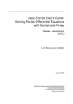
Figure 3.10: Convergence verified for Case 1 (linear problem) and Case 2 (nonlinear
problem).
For different time dependent PDEs, an ESDIRK method was used to integrate the system
in time with a very small, fixed step size. This was used as an approximation to the
exact solution to the semidiscretized system. The same system was then integrated over
44
the same time domain with a variety of greater step sizes. These solutions was then
compared with the highly refined solution in order to get an estimate for the global error.
When using an ESDIRK method whose advancing method has order p, we should expect
that the error, when plotted in a loglog-plot, assumes a linear relation with slope p.
Case 1: The Heat Equation and Case 2: The Fisher-Kolmogorov Equation will be considered to verify that the ESDIRK implementation converges correctly for both the linear
and nonlinear problems.
For both cases, ESDIRK43a with step size ∆t = 2−11 was used to produce the approximation to the exact solution of the semidiscretized system. This solution was then
compared with solutions produced using time steps ∆t = 2−i for i = 4, . . . , 9. For the
nonlinear case, the convergence criterion for the Newton iterations was set to near machine precision in an attempt to eliminate significant error contributions. The results of
these experiments can be found in figure 3.10a and 3.10b which show that the convergence is as expected.
3.4 Verification of Constructive Step Size Selection
Gryphon comes equipped with two different step size selectors (see chapter 1.7 for details). The following experiment sought to investigate how the two step size selectors
performed compared to each other. To test this, each step size selector was applied to
Case 3: The Gray-Scott model with parameters selected to produce the bubble-pattern
and Case 4: A FitzHugh-Nagumo Reaction-Diffusion model. Output from the ESDIRK
module can be found in figure 3.11 and 3.12 and in table 3.8. From these figures we
see that the standard step size selector is unable to handle dramatic step size reductions
without rejecting every other step. The step size selector by Gustafsson, on the other
hand, is able to handle this situation better, which is as expected.
3.5 Run Time Statistics
The following experiment sought to verify that the implemented ESDIRK methods behaved as expected when subjected to linear/nonlinear problems for different tolerances
and step size selectors. Test Case 1: The Heat Equation and Test Case 2: The FisherKolmogorov Equation will be revisited. We of course expect the solver to perform better
with respect to run time on the linear problem, than the nonlinear. It is also of interest to
verify that the global error is well behaved with respect to the user specified time stepping tolerance. We would like our solver to behave such that a way that the global error
45
is reduced proportional to a reduction in the tolerance.
Both the test cases were discretized on a 49 ×49 grid using first order Lagrange elements
(502 nodes). The convergence criterion for the time integration was set to absolute.
As stepsize selectors, both the standard and the Gustafsson selector was tested with pessimistic factor P = 0.90. To generate the reference solution, ESDIRK4/3a was used
with convergence criterion for the time integration set to absolute with absolute tolerance set to 10−8 .
Table 3.9/3.10 and 3.11/3.12 shows the results for Case 1 and Case 2 using the standard/Gustafsson stepsize selector. As these tables show, it is clearly advantageous to use
local extrapolation since it provides a more accurate solution. The reduction in global
error is as desired for both the linear and nonlinear case using both the standard and the
Gustafsson stepsize selector. For ESDIRK3/2b, the amount of rejected steps using the
Gustafsson stepsize selector is significantly higher than for any other ESDIRK-method.
This effect can be explained by the fact that the stability function for the error estimate
of this method fails to satisfy |R̂(∞)| < 17 .
3.6
Comparison to Trapezoidal Rule
The trapezoidal rule is a popular second order, A-stable, Runge-Kutta method. It has
a relatively simple Butcher tableau which can be found in table 3.7. As this table sug0
1
0
1/2
1/2
0
1/2
1/2
Table 3.7: The Butcher tableau for the Trapezoidal rule.
gests, the method consists of one explicit stage and one implicit, which is significantly
less computationally demanding then for example ESDIRK4/3a which has one explicit
stage and four implicit. The following experiment sought to investigate whether or not
an ESDIRK method was able to produce as accurate solutions as the trapezoidal rule,
when allowed to use approximately the same amount of CPU time. We will compare
performance on a ODE problem and a DAE problem. As ODE problem, case 3: The
Gray-Scott model was used with parameters selected to produce the dot pattern (see table 3.5) on the time domain t ∈ [0, 200] and t ∈ [0, 1000]. As DAE problem, case 5: The
7 Kværnø has noted this in her article where she suggests that the estimate for local error could be stabilized
by multiplying it with (I − ∆t γ0 J)−1 where γ0 is some constant and J is the Jacobian of the equation. This
"trick" originates from [HW10, Section IV.8].
46
Cahn-Hilliard equation was used on the time domain t ∈ [0, 4 · 10−4 ].
The experiment was carried out in the following way.
• Produce a highly refined solution to be used when approximating the global error.
• Solve the problem with the trapezoidal rule for various fixed time steps.
• Solve the problem with an ESDIRK method for various tolerances.
The highly refined solution was, in both cases, produced using ESDIRK4/3a with convergence criterion set to "absolute" and absolute tolerance set to 10−8 . The tolerance for
the Newton solver was set to near machine precision.
The results of this experiment for case 3 can be found in table 3.13, 3.14, 3.15 and 3.16
where CPU time (CPU), wall time (WTM), maximum global error (MGE), number of
timesteps performed, number of function evaluations (F) and number of Jacobian evaluations (J) are shown. As these tables show, the Trapezoidal rule is able to compete with
ESDIRK4/3a for crude tolerances in terms of CPU-time/global error. This is however
not the case when we look at a larger time interval (T = [0, 1000]) and require increased
accuracy. ESDIRK4/3a then clearly performs better and is able to produce a solution
which is ten times more accurate than what the Trapezoidal rule is able to produce,
using approximately half of the CPU/wall time (compare last row in table 3.15/3.16).
The results of this experiment for case 5 can be found in table 3.17 and 3.18 and we see
that ESDIRK clearly outperforms the Trapezoidal Rule. This behavior can be explained
by the fact that the specified initial data fail to be consistent. As a result of this, the
Trapezoidal Rule, which is not L-stable, will get a significant contribution to the error in
the first time step (see equation 1.9).
47
Step size selector: standard
Avg. step size
Selected step sizes
Rejected step sizes
Step size dt
0.20
0.15
0.10
0.05
0
20
40
Time t
60
80
(a) Using standard step size selector.
Step size selector: Gustafsson
0.25
Avg. step size
Selected step sizes
Rejected step sizes
Step size dt
0.20
0.15
0.10
0.05
0
20
40
Time t
60
80
(b) Using Gustafsson step size selector.
Figure 3.11: Selected step sizes for Case 4: A FitzHugh-Nagumo Reaction-Diffusion
model.
48
Step size selector: standard
Avg. step size
Selected step sizes
Rejected step sizes
Step size dt
150
100
50
0
2000
4000
6000
8000
Time t
10000
12000
14000
(a) Using standard step size selector.
Step size selector: Gustafsson
200
Avg. step size
Selected step sizes
Rejected step sizes
Step size dt
150
100
50
0
2000
4000
6000
8000
Time t
10000
12000
14000
(b) Using Gustafsson step size selector.
Figure 3.12: Selected step sizes for Case 3: The Gray-Scott model with bubble pattern
parameters.
49
CPU/wall time
No.accepted/rejected steps
Convergence criterion
Absolute/relative tolerance
Pessimistic factor
Step size selector
Function/Jacobian calls
tmin /tmax
tmean /tvar
1451.69/0:23:38
891 (94.99%)/47 (5.01%)
absolute
0.0001/1e-06
0.95
standard
11324/7572
0.001/0.24282
0.112319/0.00111999
(a) Results using ESDIRK43a on domain (0,50). Using standard step size selector, Case 4 with target pattern.
CPU/wall time
No.accepted/rejected steps
Convergence criterion
Absolute/relative tolerance
Pessimistic factor
Step size selector
Function/Jacobian calls
tmin /tmax
tmean /tvar
1390.95/0:22:42
887 (98.23%)/16 (1.77%)
absolute
0.0001/1e-06
0.95
Gustafsson
10915/7303
0.001/0.25098
0.112813/0.00120819
(b) Results using ESDIRK43a on domain (0,50). Using
Gustafsson step size selector, Case 4 with target pattern.
CPU/wall time
No.accepted/rejected steps
Convergence criterion
Absolute/relative tolerance
Pessimistic factor
Step size selector
Function/Jacobian calls
tmin /tmax
tmean /tvar
507.13/0:08:05
488 (94.21%)/30 (5.79%)
absolute
0.0001/1e-06
0.85
standard
7810/5738
0.001/185.788
30.67/1268.62
(c) Results using ESDIRK43a on domain (0,15000). Using
standard step size selector, Case 3 with bubble pattern.
CPU/wall time
No.accepted/rejected steps
Convergence criterion
Absolute/relative tolerance
Pessimistic factor
Step size selector
Function/Jacobian calls
tmin /tmax
tmean /tvar
483.97/0:07:44
472 (96.33%)/18 (3.67%)
absolute
0.0001/1e-06
0.85
Gustafsson
7465/5505
0.001/200
31.8009/1396.81
(d) Results using ESDIRK43a on domain (0,15000). Using
Gustafsson step size selector, Case 3 with bubble pattern.
Table 3.8: Run time statistics complementing figure 3.11 and 3.12.
50
Method
ESDIRK43a
ESDIRK43b
ESDIRK32a
ESDIRK32b
TOL
10−2
10−3
10−4
10−5
10−6
10−2
10−3
10−4
10−5
10−6
10−2
10−3
10−4
10−5
10−6
10−2
10−3
10−4
10−5
10−6
CPU
1.41
2.47
4.37
7.74
13.56
1.16
2.00
3.60
6.48
11.34
1.24
2.52
5.23
10.96
23.67
1.01
2.04
4.17
8.73
18.30
REJ
0
0
0
0
0
0
0
0
2
2
0
0
0
0
0
0
0
1
1
1
ACC
11
20
36
63
112
9
16
29
51
91
14
29
61
128
274
11
23
47
100
212
MGE
8.56972e-05
9.51104e-06
1.40821e-06
1.47382e-07
1.82645e-08
3.13776e-04
7.12935e-05
1.32331e-05
2.31339e-06
4.20631e-07
4.14390e-05
4.34604e-06
4.89570e-07
5.19361e-08
5.22892e-09
7.62485e-04
1.76441e-04
3.92444e-05
8.50711e-06
1.83872e-06
Table 3.9: Case 1: The Heat Equation, standard stepsize selector.
Method
ESDIRK43a
ESDIRK43b
ESDIRK32a
ESDIRK32b
TOL
10−2
10−3
10−4
10−5
10−6
10−2
10−3
10−4
10−5
10−6
10−2
10−3
10−4
10−5
10−6
10−2
10−3
10−4
10−5
10−6
CPU
1.39
2.11
3.89
6.99
12.85
1.36
2.00
3.32
5.98
10.78
1.18
2.38
4.93
10.65
23.07
1.30
2.51
5.01
10.10
21.53
REJ
2
1
1
0
0
2
2
1
2
2
1
1
0
0
0
3
7
12
18
38
ACC
9
16
31
58
107
8
14
26
47
87
12
26
57
124
269
11
22
47
99
213
MGE
9.40667e-05
1.17102e-05
1.47787e-06
1.77092e-07
1.77143e-08
4.54981e-04
7.95169e-05
1.52189e-05
2.46546e-06
4.31213e-07
4.29667e-05
4.65070e-06
5.06088e-07
5.20707e-08
5.26237e-09
8.34979e-04
1.80384e-04
3.85343e-05
8.35449e-06
1.79763e-06
Table 3.10: Case 1: The Heat Equation, Gustafsson stepsize selector
51
Method
ESDIRK43a
ESDIRK43b
ESDIRK32a
ESDIRK32b
TOL
10−2
10−3
10−4
10−5
10−6
10−2
10−3
10−4
10−5
10−6
10−2
10−3
10−4
10−5
10−6
10−2
10−3
10−4
10−5
10−6
CPU
6.85
10.63
14.79
26.21
43.63
6.04
8.68
11.80
21.39
35.05
6.40
10.16
21.12
42.77
87.64
5.16
7.83
16.71
33.32
68.12
REJ
0
0
0
1
2
0
0
0
1
1
0
0
1
1
2
1
0
1
2
2
ACC
17
27
46
82
147
15
22
37
66
117
22
44
92
198
425
17
34
72
154
329
MGE
1.57370e-03
1.31066e-04
1.13467e-05
1.02636e-06
9.74272e-08
2.53641e-03
8.32247e-04
1.41376e-04
2.42187e-05
4.19581e-06
5.03430e-04
4.59702e-05
4.39966e-06
4.32061e-07
4.16067e-08
4.27114e-03
9.30985e-04
2.02401e-04
4.38003e-05
9.46558e-06
Table 3.11: Case 2: The Fisher-Kolmogorov Equation, standard stepsize selector.
Method
ESDIRK43a
ESDIRK43b
ESDIRK32a
ESDIRK32b
TOL
10−2
10−3
10−4
10−5
10−6
10−2
10−3
10−4
10−5
10−6
10−2
10−3
10−4
10−5
10−6
10−2
10−3
10−4
10−5
10−6
CPU
5.89
10.08
13.80
25.31
42.71
5.85
8.77
11.20
20.33
34.35
6.26
9.43
20.65
42.03
87.05
6.44
9.89
19.36
39.18
79.14
REJ
0
1
0
1
2
0
2
0
1
1
1
0
1
1
2
6
9
13
28
64
ACC
14
24
43
79
143
14
20
35
63
115
20
41
90
195
423
17
34
71
154
333
MGE
1.94109e-03
1.54366e-04
1.25726e-05
1.07417e-06
9.87964e-08
2.90268e-03
8.74712e-04
1.53068e-04
2.51366e-05
4.27497e-06
5.75900e-04
4.95075e-05
4.52694e-06
4.36589e-07
4.05236e-08
4.13258e-03
9.14550e-04
1.99556e-04
4.28894e-05
9.25742e-06
Table 3.12: Case 2: The Fisher-Kolmogorov Equation, Gustafsson stepsize selector.
52
TOL
10−2
10−3
10−4
10−5
10−6
CPU
48.53
75.44
104.40
172.10
305.42
WTM
0:00:46
0:01:11
0:01:39
0:02:43
0:04:49
MGE
4.51007e-04
4.79235e-05
5.67949e-06
6.15685e-07
8.26995e-08
# steps
38
61
101
174
304
F
529
831
1198
1992
3527
J
377
587
794
1296
2311
Table 3.13: Case 3, ESDIRK4/3a on domain t ∈ [0, 200].
∆t
1.0
0.8
0.4
0.2
0.1
CPU
46.17
57.48
114.19
164.67
265.94
WTM
0:00:43
0:00:54
0:01:47
0:02:35
0:04:11
MGE
9.95809e-05
6.37574e-05
1.59479e-05
5.44435e-06
1.66880e-06
# steps
200
250
500
1000
2000
F
600
750
1500
2401
4215
J
400
500
1000
1401
2215
Table 3.14: Case 3, Trapezoidal Rule on domain t ∈ [0, 200].
TOL
10−2
10−3
10−4
10−5
10−6
CPU
105.21
172.84
263.65
417.86
766.28
WTM
0:01:39
0:02:44
0:04:09
0:06:36
0:12:05
MGE
6.64926e-04
1.02003e-04
1.21198e-05
1.26448e-06
1.25009e-07
# steps
73
128
226
408
741
F
1121
1903
2940
4800
8771
J
829
1391
2036
3168
5807
Table 3.15: Case 3, ESDIRK4/3a on domain t ∈ [0, 1000].
∆t
2.5
0.8
0.4
0.2
0.1
CPU
93.20
286.49
493.48
645.63
1234.43
WTM
0:01:27
0:04:29
0:07:43
0:10:09
0:19:24
MGE
9.05509e-04
9.30402e-05
2.41657e-05
7.43637e-06
2.04581e-06
# steps
400
1250
2500
5000
10000
F
1208
3750
6757
10401
20215
J
808
2500
4257
5401
10215
Table 3.16: Case 3, Trapezoidal Rule on domain t ∈ [0, 1000].
TOL
10−2
10−3
10−4
10−5
CPU
405.34
864.13
1292.01
2525.29
WTM
0:06:19
0:13:27
0:20:08
0:39:22
MGE
6.80848e-02
5.13463e-03
3.79484e-04
2.78449e-05
# steps
325
686
1427
2870
F
5106
10764
17460
34436
J
3806
8020
11752
22956
Table 3.17: Case 5, ESDIRK4/3a on domain t ∈ [0, 4 · 10−4 ]
∆t
1e-06
1e-07
5e-08
1e-08
CPU
118.63
821.53
1640.64
8194.87
WTM
0:01:50
0:12:44
0:25:25
2:07:01
MGE
6.63918e+00
2.48727e-02
1.13210e-02
2.08466e-03
# steps
400
4000
8000
40000
F
1587
12000
24000
120000
J
1187
8000
16000
80000
Table 3.18: Case 5, Trapezoidal Rule on domain t ∈ [0, 4 · 10−4 ]
53
Part IV
Gryphon User Manual
54
4.1 Introduction
This part serves as a user manual to the Gryphon module. Gryphon is intended for
use under FEniCS 1.0.0 with the Python API. This document expects that the reader is
familiar with the FEniCS framework.
4.2 Handling Explicit Time Dependency
In order for the Gryphon to recognize explicit time dependent expressions, the variable
representing time in an expression must be named t. If we want to represent the function
f (x, y,t) = x + y + t,
we can do it in two ways. The simplest way is to write
f = Expression("x[0] + x[1] + t",t=0)
or you could define a class
class f (Expression):
def eval ( self , values ,x) :
values [0] = x[0] + x[1] + self . t
Note that the variable t must be assigned an initial value.
4.3 Solver: ESDIRK
The ESDIRK class represents the realization of a collection of singly diagonally implicit
Runge-Kutta methods with an explicit first stage. It is able to handle systems of PDEs
which either semidiscretize into a pure ODE system or a DAE system of index 1.
In order to use an ESDIRK solver you first have to import it as such:
from gryphon import ESDIRK
The constructor for the ESDIRK object have three required arguments and four optional
keyword arguments. The header for the constructor is as follows:
def __init__(self,T,u,f,g=[],bcs=[], tdf =[],tdfBC=[]):
The arguments have the following interpretations:
55
T: This argument should be an array with two elements defining the start and end of
the time domain you wish to integrate over. For example, T = [0,1].
u: This argument represent the initial condition used for the time integration. It should
be given as a Function-object defined on the spatial mesh for which to integrate. When
the solver terminates, this object will contain the solution in the final time step.
f: This argument should be a Form-object representing the ODE-component of your
problem. If you are solving a system with more than one ODE-component, you can
pass a list of Form-objects corresponding to each ODE-component in the system. An
example of this can be found at the end of this document where the Gray-Scott model is
solved.
g: This argument should be a Form-object representing the DAE-component of your
problem. If you are solving a system with more than one DAE-component, you can pass
a list of Form-objects corresponding to each DAE-component in the system.
tdf: If any of the Form-objects in f or g contains explicit time dependent functions,
they must be passed to the constructor via this argument.
bcs: This argument should be a list of DirichletBC-objects or PeriodicBC-objects
defining the Dirichlet boundary conditions of your problem.
tdfBC: If any of the boundary conditions specified in f or g are explicitly dependent
on time, they must be passed to the constructor via this argument.
4.3.1 Parameters
Gryphon inherits the parameter system included in the FEniCS framework. This allows
any user familiar with FEniCS to quickly get an overview over the available parameters
for a ESDIRK-object by calling
info (ESDIRK_object.parameters, verbose=True)
By default, this will return the following output (some columns are omitted)
56
<Parameter set "gryphon" containing 3 parameter(s)>
gryphon |
type
value
−−−−−−−−−−−−−−−−−−−−−−−−−−−−−−
drawplot |
bool
false
method
| string ESDIRK43a
verbose
|
bool
false
<Parameter set "output" containing 3 parameter(s)>
output
|
type
value
−−−−−−−−−−−−−−−−−−−−−−−−−−−−−−−−−
path
| string outputData
plot
|
bool
false
statistics
|
bool
false
<Parameter set "timestepping" containing 10 parameter(s)>
timestepping
|
type
value
−−−−−−−−−−−−−−−−−−−−−−−−−−−−−−−−−−−−−−−−−−−−−
absolute_tolerance
| double
1e−07
adaptive
|
bool
true
convergence_criterion
| string absolute
dt
| double
0.15
dtmax
| double
15
dtmin
| double
1e−14
inconsistent_initialdata
|
bool
false
pessimistic_factor
| double
0.8
relative_tolerance
| double
1e−06
stepsizeselector
| string standard
It should be noted that the parameter sets "output" and "timestepping" are nested under
the parameter set "gryphon". This means that if we for instance would like to turn
off adaptive time stepping, turn on plotting and save statistics, we have to write the
following:
ESDIRK_object.parameters["timestepping"]["adaptive"] = False
ESDIRK_object.parameters["drawplot"] = True
ESDIRK_object.parameters["output"][" statistics "] = True
The various parameters have the following interpretations:
Parameter set: gryphon
method (Default value: "ESDIRK43a") This parameter defines which ESDIRK method
the program should use when doing the time stepping. Available methods to choose from
are ESDIRK43a, ESDIRK43b, ESDIRK32a, ESDIRK32b. For details on these methods, see table 4.19
57
Name
ESDIRK4/3a
ESDIRK4/3b
ESDIRK3/2a
ESDIRK3/2b
Order
4
3
3
2
Implicit Stages
4
4
3
3
Local Extrapolation
Yes
No
Yes
No
Table 4.19: Details on available ESDIRK methods
drawplot (Default value: False) If this parameter is set to True, the program will
display a plot of the solution in each time step using the built in plot-function included
in the FEniCS framework. Note that the plot is initialized with the keyword argument
rescale=True.
verbose (Default value: False) If this parameter is set to True, the program will
output a progress bar showing the progress of the time stepping. Example output can be
found in listing 4.4. Upon completion, it will also cause the program to print the same
statistics as found in listing 4.5 to screen.
|====>...............
|====>...............
|====>...............
|====>...............
|====>...............
|=====>..............
|=====>..............
|
|
|
|
|
|
|
27.2%
27.3%
27.3%
27.4%
27.4%
27.5%
27.6%
t=2.722
t=2.728
t=2.733
t=2.739
t=2.744
t=2.750
t=2.755
Completion
Completion
Completion
Completion
Completion
Completion
Completion
in
in
in
in
in
in
in
~
~
~
~
~
~
~
0:03:42
0:03:44
0:03:30
0:03:22
0:03:36
0:03:23
0:03:37
Listing 4.4: Example output from verbose=True
The estimated run time of the program is calculated as
Run time ≈
Wall time in previous iteration
· (tend − tn )
Average of selected time steps
(4.23)
where tend is the end of the time domain and tn is the current time in time step n. Because
this estimate is dependent on the average of currently selected time steps, the estimate is
not shown before the time stepping process has proceeded 1%.
Parameter set: output
path (Default value: outputData) This parameter defines the path to a folder where
the program may save output, relative to the current working directory. Usually, this
will result in a folder outputData being created in the same folder as the script you are
running.
58
plot (Default value: False) If this parameter is set to True, the program will export
a plot of the solution in each time step to VTK-format. If you are solving a system of
PDEs, each component will be saved separately. The plots will be saved in the following
folder:
$ current_working_directory/savepath/plot/
statistics (Default value: False) If this parameter is set to True, the program will
output statistics to an .tex-file and a ascii-file as well as saving a plot of the selected
step sizes. Example output can be seen below in table 4.21, listing 4.5 and figure 4.13.
All the data will be saved to the path defined by the parameter path.
Parameter set: timestepping
adaptive (Default value: True) This parameter indicates whether the program should
use adaptive step size selection. If set to False, fixed time step integration will be used
where the fixed time step is defined by the parameter dt.
convergence_criterion (Default value: "absolute") When deciding whether or not
to accept a time step, the estimated local error can be subject to one of two user specified criteria; "absolute" or "relative". If convergence_criterion = "absolute",
the step is accepted if
ken k2 ≤ absolute_tolerance.
If convergence_criterion = "relative" the step is accepted if
ken k2 ≤ max{relative_convergence · kun k2 , absolute_convergence}.
In the above statements, en is the estimate for the local error and un is the numerical
solution in time step n.
absolute_tolerance (Default value: 1e-7) See convergence_criterion for more details.
relative_tolerance (Default value: 1e-6) See convergence_criterion for more details.
59
dt (Default value: one thousandth of the time domain) This parameter defines the
initial time step used by the program. If the parameter adaptive is set to True, this is
the time step used by the program through the entire domain.
dtmax (Default value: one tenth of the time domain) This parameter defines the
greatest allowable time step which the program can use.
dtmin (Default value: 1e-14) This parameter defines the smallest allowable time step
which the program can use. The program will terminate if this boundary is reached (not
sure about this yet).
inconsistent_initialdata (Default value: False) If the initial data for solving a system of PDEs (which semidiscretize into a DAE system) is inconsistent, the program can
attempt to take a very small time step in order to get consistent data. If successful, the
program will continue with the initial time step specified by dt.
pessimistic_factor (Default value: 0.8) This parameter defines the pessimistic factor
used in the adaptive step size selection. Allowable range for this parameter is [0, 1]. See
stepsizeselector for more details.
stepsizeselector (Default value standard) This parameter allows the user to select
which time step selecting algorithm to use. The available methods are listed in table
4.20.
Method
gustafsson
standard
Expression
(
)
∆tn2
P · tol · len−1 1/p
∆tn+1 =
∆tn−1
le2n
(
)
P · tol 1/p
∆tn+1 = ∆tn
len
Table 4.20: Available time step algorithms.
The gustafsson step size selector is developed by K. Gustafsson [Gus94].
60
4.3.2 Example Output
If the parameter savestatistics=True for an ESDIRK-object, the program will, if
it terminated successfully, produce a LATEX/ASCII-table with some relevant run time
statistics as well as a plot of the selected time steps. Examples of this output can be seen
in table 4.21, listing 4.5 and figure 4.13. The statistics were generated by running the
heat equation example presented in the next section.
∗∗∗∗∗∗∗∗∗∗∗∗∗∗∗∗∗∗∗∗∗∗∗∗∗∗∗∗∗∗∗∗∗∗∗∗∗∗∗∗∗∗∗∗
ODE solver terminated successfully !
∗∗∗∗∗∗∗∗∗∗∗∗∗∗∗∗∗∗∗∗∗∗∗∗∗∗∗∗∗∗∗∗∗∗∗∗∗∗∗∗∗∗∗∗
Method used: ESDIRK43a
Domain:
[0,1]
CPU−time: 11
Walltime:
0:00:13
Step size selector : standard
Pessimistic factor : 0.8
Convergence criterion : absolute
Absolute tolerance : 1e−07
Relative tolerance : 1e−06
Number of steps accepted: 193 (98.97%)
Number of steps rejected : 2 (1.03%)
Maximum step size selected : 0.0118945
Minimum step size selected : 0.000177563
Mean step size : 0.00517595
Variance in step sizes : 1.40139e−05
Listing 4.5: Example output from savestatistics=True.
CPU/wall time
No.accepted/rejected steps
Convergence criterion
Absolute/relative tolerance
Pessimistic factor
Step size selector
tmin /tmax
tmean /tvar
11/0:00:13
193 (98.97%)/2 (1.03%)
absolute
1e-07/1e-06
0.8
standard
0.000177563/0.0118945
0.00517595/1.40139e-05
Table 4.21: Results using ESDIRK43a on domain [0,1].
61
Step size selector: standard
0.012
Avg. step size
Selected step sizes
Rejected step sizes
0.010
Step size dt
0.008
0.006
0.004
0.002
0.0
0.2
0.4
Time t
0.6
0.8
Figure 4.13: Example output from savestatistics=True.
4.4
Example Problems
This section will show some code examples for solving time dependent partial differential equations. It is assumed that the reader is familiar with the FEniCS framework as
well as being able to derive the weak solution of a PDE.
62
The Heat Equation
Consider the heat equation with a source term given as
[
]
(π )
∂u
(x − 0.7)2 + (y − 0.5)2
= Du ∇2 u + 10 sin
t exp −
,
∂t
2
0.01
u ∈ Ω,
with diffusion coefficient Du = 0.1 and boundary/initial conditions given as
u(0, y,t) = t,
u(1, y,t) = 0,
u(x, y, 0) = 0,
on the spatial domain Ω = [0, 1] × [0, 1] and time domain t ∈ [0, 1]. The FEniCS code for
solving this problem using the ESDIRK module can be found in listing 4.6.
63
from gryphon import ESDIRK
from dolfin import ∗
# Define spatial mesh, function space, trial / test functions
mesh = UnitSquare(29,29)
V = FunctionSpace(mesh,"Lagrange",1)
u = TrialFunction(V)
v = TestFunction(V)
# Define diffusion coefficient and source inside domain
D = Constant(0.1)
domainSource = Expression("10∗sin(pi/2∗t)∗exp(−((x[0]−0.7)∗(x[0]−0.7) + (x[1]−0.5)∗(x
[1]−0.5))/0.01)",t=0)
# Define right hand side of the problem
rhs = −D∗inner(grad(u),grad(v))∗dx + domainSource∗v∗dx
# Definie initial condition
W = Function(V)
W.interpolate (Constant(0.0))
# Define left and right boundary
def boundaryLeft(x,on_boundary):
return x [0] < DOLFIN_EPS
def boundaryRight(x,on_boundary):
return 1.0 − x[0] < DOLFIN_EPS
boundarySource = Expression("t",t=0)
bcLeft = DirichletBC(V,boundarySource,boundaryLeft)
bcRight = DirichletBC(V,0.0,boundaryRight)
# Define the time domain
T = [0,1]
# Create the ESDIRK object
obj = ESDIRK(T,W,rhs,bcs=[bcLeft,bcRight],tdfBC=[boundarySource],tdf=[domainSource])
# Turn on some output and save run time
# statistics to sub folder "HeatEquation"
obj .parameters["verbose"] = True
obj .parameters["drawplot"] = True
obj .parameters["output"]["path"] = "HeatEquation"
obj .parameters["output"][" statistics "] = True
# Solve the problem
obj . solve ()
Listing 4.6: FEniCS code for solving the heat equation with time dependent source term
and time dependent boundary.
64
The Gray-Scott model
The Gray-Scott model is a nonlinear reaction-diffusion system which consist of a coupled system of two partial differential equations given as
∂u
= Du ∇2 u − uv2 + F(1 − u),
∂t
∂v
= Dv ∇2 v + uv2 − (F + k)v,
∂t
where
Du , Dv , F, k ∈ R.
We want to solve this system using the parameters Du = 8.0 · 10−5 , Dv = 4.0, ·10−5 ,
F = 0.024, k = 0.060 on the spatial domain Ω = [0, 2] × [0, 2] over the time domain
t ∈ [0, 100], with homogeneous Neumann boundary conditions and initial conditions
given as
u(x, y, 0) = 1 − 2v(x, y, 0),
{
0.25 sin2 (4π x) sin2 (4π y) if 0.75 ≤ x, y ≤ 1.25,
v(x, y, 0) =
0
elsewhere.
The FEniCS code for solving this problem using the ESDIRK module can be found in
listing 4.7.
65
from gryphon import ESDIRK
from dolfin import ∗
from numpy import power,pi,sin
class InitialConditions (Expression):
def eval ( self , val , x) :
if between(x [0],(0.75,1.25) ) and between(x [1],(0.75,1.25) ) :
val [1] = 0.25∗power(sin(4∗pi∗x [0]) ,2)∗power(sin(4∗pi∗x [1]) ,2)
val [0] = 1 − 2∗val[1]
else :
val [1] = 0
val [0] = 1
def value_shape(self ) :
return (2,)
# Define mesh, function space and test functions
mesh = Rectangle(0.0, 0.0, 2.0, 2.0, 49, 49)
V = FunctionSpace(mesh, "Lagrange", 1)
ME = V∗V
q1,q2 = TestFunctions(ME)
# Define and interpolate initial condition
W = Function(ME)
W.interpolate ( InitialConditions ())
u,v = split (W)
# Define parameters in Gray−Scott model
Du = Constant(8.0e−5)
Dv = Constant(4.0e−5)
F = Constant(0.024)
k = Constant(0.06)
# Define the right hand side for each of the PDEs
F1 = (−Du∗inner(grad(u),grad(q1)) − u∗(v∗∗2)∗q1 + F∗(1−u)∗q1)∗dx
F2 = (−Dv∗inner(grad(v),grad(q2)) + u∗(v∗∗2)∗q2 − (F+k)∗v∗q2)∗dx
# Define the time domain
T = [0,100]
# Create the solver object and adjust tolerance
obj = ESDIRK(T,W,[F1,F2])
obj .parameters["timestepping" ][ "absolute_tolerance"] = 1e−3
# Turn on some output and save run time
# statistics to sub folder "GrayScott"
obj .parameters["verbose"] = True
obj .parameters["drawplot"] = True
obj .parameters["output"]["path"] = "GrayScott"
obj .parameters["output"][" statistics "] = True
# Suppress some FEniCS output
set_log_level(WARNING)
# Solve the problem
obj . solve ()
Listing 4.7: FEniCS code for solving the Gray-Scott model.
66
The Cahn-Hilliard equation
The Cahn-Hilliard equation is used to model how the mixture of two binary fluids can
separate and form domains pure in each component. The equation can be written as the
following system
∂u
= M∇2 v,
∂t
df
0 = v−
− λ ∇2 u,
du
which, when discretized, will result in a DAE system of index 1. We will consider
the case when M = 1.0, λ = 1 · 10−2 and f = 100u2 (1 − u2 ) on the spatial domain
Ω = [0, 1] × [0, 1] with homogeneous Neumann boundary conditions. In time, we will
consider the domain t ∈ [0, 4 · 10−4 ]. The following initial conditions will be used
u(x, y) = 0.63 + 0.02 · (0.5 − χ ),
χ ∼ Uni f [0, 1],
v(x, y) = 0.
The FEniCS code for solving this problem using the ESDIRK module can be found in
listing 4.8
67
from gryphon import ESDIRK
from dolfin import ∗
import random
# Initial conditions
class InitialConditions (Expression):
def __init__(self):
random.seed(2 + MPI.process_number())
def eval ( self , values , x) :
values [0] = 0.63 + 0.02∗(0.5 − random.random())
values [1] = 0.0
def value_shape(self ) :
return (2,)
# Create mesh and define function spaces
mesh = UnitSquare(49, 49)
V = FunctionSpace(mesh, "Lagrange", 1)
ME = V∗V
q,v = TestFunctions(ME)
# Define and interpolate initial condition
u = Function(ME)
u. interpolate ( InitialConditions ())
c,mu = split(u)
c = variable (c)
f
= 100∗c∗∗2∗(1−c)∗∗2
dfdc = diff ( f , c)
lmbda = Constant(1.0e−02)
# Weak statement of the equations
f = −inner(grad(mu), grad(q))∗dx
g = mu∗v∗dx − dfdc∗v∗dx − lmbda∗inner(grad(c), grad(v))∗dx
T = [0,5e−5] # Time domain
myobj = ESDIRK(T,u,f,g=g)
myobj.parameters[’ timestepping ’ ][ ’ absolute_tolerance ’ ] = 1e−2
myobj.parameters[’ timestepping ’ ][ ’ inconsistent_initialdata ’ ] = True
myobj.parameters[’ verbose ’ ] = True
myobj.parameters[’drawplot’ ] = True
# Suppress some FEniCS output
set_log_level(WARNING)
# Solve the problem
myobj.solve()
Listing 4.8: FEniCS code for solving the the Cahn-Hilliard equation.
68
Summary of Results
After considering various Runge-Kutta schemes for solving stiff ODEs, the ESDIRK
methods developed by Anne Kværnø were found to be suitable. The idea of using these
methods as time integrators when solving time dependent partial differential equations,
gave rise to the Gryphon module.
The code structure of Gryphon focuses on modularity. Adding a new time integrator
scheme only requires writing the code for augmenting a user-specified problem (specified in UFL) with the code amounting to applying the desired time integrator, and the
code for performing the time stepping loop. Tools like time stepping algorithms are already available and can be reused. The source code for the ESDIRK solvers are well
documented (see attachment A) and aims to serve as guidance for people who wants to
extend the framework with their own time integrators.
The ESDIRK methods have been tested on various time dependent PDEs, verifying
that the methods converge correctly and are able to compete with other time integrators
(Trapezoidal rule), when it comes to numerical accuracy versus run time. It has also been
verified that the step size selectors behave as expected by subjecting them to reactiondiffusion problems.
Numerous code examples have also been presented, hopefully motivating the reader to
try and use Gryphon for solving his/her own problems.
69
Appendix
A
Appended Code and
Documentation
Together with this document you should have received an attached zip file called gryphon
_appendix.zip. This file contains the following:
documentation/
This folder contains the documentation for Gryphon. To start, open the file Gryphon.html
in any web browser (Firefox/Chrome looks good).
source/
This folder contains the source code for the Gryphon module. In order to use Gryphon,
this folder must be included in your Python-path.
examplecode/
This folder contains the Python code for the examples found in the Gryphon user manual.
reportcode/
This folder contains the Python code for the example presented in section II.2.4.
70
Bibliography
[BCP89]
K.E. Brenan, S.L. Campbell, and L.R. Petzold, Numerical solution of
initial-value problems in differential-algebraic equations, Classics in Applied Mathematics, Society for Industrial and Applied Mathematics, 1989.
[EJL03]
K. Eriksson, C. Johnson, and A. Logg, Explicit time-stepping for stiff ODEs,
SIAM Journal on Scientific Computing 25 (2003), 1142.
[Gus94]
K. Gustafsson, Control-theoretic techniques for stepsize selection in implicit Runge-Kutta methods, ACM Transactions on Mathematical Software
(TOMS) 20 (1994), no. 4, 496–517.
[HT99]
A. Hunt and D. Thomas, The pragmatic programmer: From journeyman to
master, Pearson Education, 1999.
[HV03]
W.H. Hundsdorfer and J.G. Verwer, Numerical solution of time-dependent
advection-diffusion-reaction equations, vol. 33, Springer Verlag, 2003.
[HW10]
E. Hairer and G. Wanner, Solving ordinary differential equations. ii: Stiff and
differential-algebraic problems., Springer Series in Computational Mathematics 14. Berlin: Springer. xvi, 614 p., 2010.
[KNO96] A. Kværnø, SP Nørsett, and B. Owren, Runge-Kutta research in Trondheim,
Applied numerical mathematics 22 (1996), no. 1, 263–277.
[Kvæ04]
A. Kværnø, Singly diagonally implicit Runge-Kutta methods with an explicit
first stage, BIT Numerical Mathematics 44 (2004), no. 3, 489–502.
[LMW11] A. Logg, K.A. Mardal, and G. Wells, Automated solution of differential equations by the finite element method: The fenics book, 2011.
71
[Mun12]
R. Munafo, Reaction-diffusion by the Gray-Scott model: Pearson’s parameterization, http://mrob.com/pub/comp/xmorphia/, April 2012.
[NT84]
S.P. Nørsett and P.G. Thomsen, Embedded SDIRK-methods of basic order
three, BIT Numerical Mathematics 24 (1984), no. 4, 634–646.
[Pro12a]
The FEniCS Project, Cahn-hilliard equation, http://fenicsproject.
org/documentation/dolfin/1.0.0/python/demo/pde/
cahn-hilliard/python/documentation.html, May 2012.
[Pro12b]
, Time-dependent problem, tutorial, http://fenicsproject.
org/documentation/tutorial/timedep.html, May 2012.
72