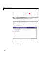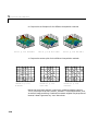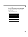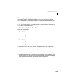
1
MATLAB ® The Language of Technical Computing Computation Visualization Programming Using MATLAB Version 5 How to Contact The MathWorks: 508-647-7000 Phone 508-647-7001 Fax The MathWorks, Inc. 24 Prime Park Way Natick, MA 01760-1500 Mail http://www.mathworks.com Web Anonymous FTP server Newsgroup ftp.mathworks.com comp.soft-sys.matlab [email protected] [email protected] [email protected] [email protected] [email protected] [email protected] [email protected] Technical support Product enhancement suggestions Bug reports Documentation error reports Subscribing user registration Order status, license renewals, passcodes Sales, pricing, and general information Using MATLAB COPYRIGHT 1984 - 1999 by The MathWorks, Inc. The software described in this document is furnished under a license agreement. The software may be used or copied only under the terms of the license agreement. No part of this manual may be photocopied or reproduced in any form without prior written consent from The MathWorks, Inc. U.S. GOVERNMENT: If Licensee is acquiring the Programs on behalf of any unit or agency of the U.S. Government, the following shall apply: (a) For units of the Department of Defense: the Government shall have only the rights specified in the license under which the commercial computer software or commercial software documentation was obtained, as set forth in subparagraph (a) of the Rights in Commercial Computer Software or Commercial Software Documentation Clause at DFARS 227.7202-3, therefore the rights set forth herein shall apply; and (b) For any other unit or agency: NOTICE: Notwithstanding any other lease or license agreement that may pertain to, or accompany the delivery of, the computer software and accompanying documentation, the rights of the Government regarding its use, reproduction, and disclosure are as set forth in Clause 52.227-19 (c)(2) of the FAR. MATLAB, Simulink, Stateflow, Handle Graphics, and Real-Time Workshop are registered trademarks, and Target Language Compiler is a trademark of The MathWorks, Inc. COPYRIGHT 1995 Bristol Technology, Inc. All rights reserved. COPYRIGHT 1995 Microsoft Corporation. All rights reserved. Other product or brand names are trademarks or registered trademarks of their respective holders. Printing History: December 1996 June 1997 January 1998 January 1999 First printing for MATLAB 5.0 Revised for MATLAB 5.1 Revised for MATLAB 5.2 Revised for MATLAB 5.3 (Release 11) Contents Introduction 1 MATLAB Working Environment 2 Using the Environment . . . . . . . . . . . . . . . . . . . . . . . . . . . . . . . . 2-2 The Command Window . . . . . . . . . . . . . . . . . . . . . . . . . . . . . . . . 2-5 The Figure Window . . . . . . . . . . . . . . . . . . . . . . . . . . . . . . . . . . 2-18 Help and Online Documentation . . . . . . . . . . . . . . . . . . . . . . 2-20 Disk File Manipulation and Shell Escape . . . . . . . . . . . . . . 2-25 Data Import/Export . . . . . . . . . . . . . . . . . . . . . . . . . . . . . . . . . . 2-26 Memory Utilization . . . . . . . . . . . . . . . . . . . . . . . . . . . . . . . . . . 2-33 Microsoft Windows Handbook . . . . . . . . . . . . . . . . . . . . . . . . 2-35 UNIX Handbook . . . . . . . . . . . . . . . . . . . . . . . . . . . . . . . . . . . . . 2-54 Debugger and Profiler 3 MATLAB Debugger . . . . . . . . . . . . . . . . . . . . . . . . . . . . . . . . . . . 3-2 M-File Profiler . . . . . . . . . . . . . . . . . . . . . . . . . . . . . . . . . . . . . . . 3-17 i Matrices and Linear Algebra 4 Matrices and Linear Algebra . . . . . . . . . . . . . . . . . . . . . . . . . . . 4-2 Matrices in MATLAB . . . . . . . . . . . . . . . . . . . . . . . . . . . . . . . . . . 4-4 Solving Linear Equations . . . . . . . . . . . . . . . . . . . . . . . . . . . . . 4-13 Inverses and Determinants . . . . . . . . . . . . . . . . . . . . . . . . . . . 4-20 LU, QR, and Cholesky Factorizations . . . . . . . . . . . . . . . . . . 4-24 Matrix Powers and Exponentials . . . . . . . . . . . . . . . . . . . . . . 4-31 Eigenvalues . . . . . . . . . . . . . . . . . . . . . . . . . . . . . . . . . . . . . . . . . 4-34 Singular Value Decomposition . . . . . . . . . . . . . . . . . . . . . . . . 4-38 Polynomials and Interpolation 5 Polynomials . . . . . . . . . . . . . . . . . . . . . . . . . . . . . . . . . . . . . . . . . . 5-2 Interpolation . . . . . . . . . . . . . . . . . . . . . . . . . . . . . . . . . . . . . . . . . 5-9 Data Analysis and Statistics 6 Column-Oriented Data Sets . . . . . . . . . . . . . . . . . . . . . . . . . . . . 6-3 Basic Data Analysis Functions . . . . . . . . . . . . . . . . . . . . . . . . . 6-7 Data Pre-Processing . . . . . . . . . . . . . . . . . . . . . . . . . . . . . . . . . . 6-12 ii Contents Regression and Curve Fitting . . . . . . . . . . . . . . . . . . . . . . . . . 6-15 Case Study: Curve Fitting . . . . . . . . . . . . . . . . . . . . . . . . . . . . . 6-20 Difference Equations and Filtering . . . . . . . . . . . . . . . . . . . . 6-29 Fourier Analysis and the Fast Fourier Transform (FFT) . 6-31 Function Functions 7 Representing Functions in MATLAB . . . . . . . . . . . . . . . . . . . . 7-3 Plotting Mathematical Functions . . . . . . . . . . . . . . . . . . . . . . . 7-4 Minimizing Functions and Finding Zeros . . . . . . . . . . . . . . . . 7-7 Numerical Integration (Quadrature) . . . . . . . . . . . . . . . . . . . 7-14 Ordinary Differential Equations 8 Quick Start . . . . . . . . . . . . . . . . . . . . . . . . . . . . . . . . . . . . . . . . . . . 8-3 Representing Problems . . . . . . . . . . . . . . . . . . . . . . . . . . . . . . . . 8-5 ODE Solvers . . . . . . . . . . . . . . . . . . . . . . . . . . . . . . . . . . . . . . . . . 8-10 Creating ODE Files . . . . . . . . . . . . . . . . . . . . . . . . . . . . . . . . . . . 8-14 Improving Solver Performance . . . . . . . . . . . . . . . . . . . . . . . . 8-17 Examples: Applying the ODE Solvers . . . . . . . . . . . . . . . . . . 8-34 iii Questions and Answers . . . . . . . . . . . . . . . . . . . . . . . . . . . . . . . 8-50 Sparse Matrices 9 Introduction . . . . . . . . . . . . . . . . . . . . . . . . . . . . . . . . . . . . . . . . . . 9-5 Viewing Sparse Matrices . . . . . . . . . . . . . . . . . . . . . . . . . . . . . . 9-11 Example: Adjacency Matrices and Graphs . . . . . . . . . . . . . . 9-15 Sparse Matrix Operations . . . . . . . . . . . . . . . . . . . . . . . . . . . . . 9-23 M-File Programming 10 MATLAB Programming: A Quick Start . . . . . . . . . . . . . . . . . 10-2 Scripts . . . . . . . . . . . . . . . . . . . . . . . . . . . . . . . . . . . . . . . . . . . . . . 10-5 Functions . . . . . . . . . . . . . . . . . . . . . . . . . . . . . . . . . . . . . . . . . . . 10-6 Local and Global Variables . . . . . . . . . . . . . . . . . . . . . . . . . . . 10-16 Data Types . . . . . . . . . . . . . . . . . . . . . . . . . . . . . . . . . . . . . . . . . 10-19 Operators . . . . . . . . . . . . . . . . . . . . . . . . . . . . . . . . . . . . . . . . . . 10-21 Flow Control . . . . . . . . . . . . . . . . . . . . . . . . . . . . . . . . . . . . . . . 10-30 Subfunctions . . . . . . . . . . . . . . . . . . . . . . . . . . . . . . . . . . . . . . . 10-38 Indexing and Subscripting . . . . . . . . . . . . . . . . . . . . . . . . . . . 10-40 iv Contents String Evaluation . . . . . . . . . . . . . . . . . . . . . . . . . . . . . . . . . . . 10-46 Command/Function Duality . . . . . . . . . . . . . . . . . . . . . . . . . . 10-48 Empty Matrices . . . . . . . . . . . . . . . . . . . . . . . . . . . . . . . . . . . . . 10-49 Errors and Warnings . . . . . . . . . . . . . . . . . . . . . . . . . . . . . . . . 10-51 Times and Dates . . . . . . . . . . . . . . . . . . . . . . . . . . . . . . . . . . . . 10-54 Obtaining User Input . . . . . . . . . . . . . . . . . . . . . . . . . . . . . . . . 10-61 Shell Escape Functions . . . . . . . . . . . . . . . . . . . . . . . . . . . . . . 10-62 Optimizing the Performance of MATLAB Code . . . . . . . . . 10-63 Character Arrays (Strings) 11 Character Arrays . . . . . . . . . . . . . . . . . . . . . . . . . . . . . . . . . . . . 11-4 Cell Arrays of Strings . . . . . . . . . . . . . . . . . . . . . . . . . . . . . . . . . 11-7 String Comparisons . . . . . . . . . . . . . . . . . . . . . . . . . . . . . . . . . . 11-9 Searching and Replacing . . . . . . . . . . . . . . . . . . . . . . . . . . . . 11-12 String/Numeric Conversion . . . . . . . . . . . . . . . . . . . . . . . . . . 11-13 Multidimensional Arrays 12 Multidimensional Arrays . . . . . . . . . . . . . . . . . . . . . . . . . . . . . 12-3 v Computation with Multidimensional Arrays . . . . . . . . . . . 12-15 Organizing Data in Multidimensional Arrays . . . . . . . . . . 12-17 Multidimensional Cell Arrays . . . . . . . . . . . . . . . . . . . . . . . . 12-19 Multidimensional Structure Arrays . . . . . . . . . . . . . . . . . . . 12-20 Structures and Cell Arrays 13 Structures . . . . . . . . . . . . . . . . . . . . . . . . . . . . . . . . . . . . . . . . . . . 13-3 Cell Arrays . . . . . . . . . . . . . . . . . . . . . . . . . . . . . . . . . . . . . . . . . 13-19 MATLAB Classes and Objects 14 Classes and Objects: An Overview . . . . . . . . . . . . . . . . . . . . . 14-2 Designing User Classes in MATLAB . . . . . . . . . . . . . . . . . . . . 14-9 Overloading Operators and Functions . . . . . . . . . . . . . . . . 14-20 Example: A Polynomial Class . . . . . . . . . . . . . . . . . . . . . . . . . 14-23 Building on Other Classes . . . . . . . . . . . . . . . . . . . . . . . . . . . 14-34 Example: Assets and Asset Subclasses . . . . . . . . . . . . . . . . . 14-37 Example: The Portfolio Container . . . . . . . . . . . . . . . . . . . . 14-54 Saving and Loading Objects . . . . . . . . . . . . . . . . . . . . . . . . . . 14-61 vi Contents Object Precedence . . . . . . . . . . . . . . . . . . . . . . . . . . . . . . . . . . 14-66 How MATLAB Determines Which Method to Call . . . . . . . 14-68 File I/O 15 Opening and Closing Files . . . . . . . . . . . . . . . . . . . . . . . . . . . . 15-3 Temporary Files and Directories . . . . . . . . . . . . . . . . . . . . . . 15-6 Binary Files . . . . . . . . . . . . . . . . . . . . . . . . . . . . . . . . . . . . . . . . . 15-7 Controlling Position in a File . . . . . . . . . . . . . . . . . . . . . . . . . 15-10 Formatted Files 15-13 vii viii Contents 1 Introduction What Is MATLAB? . . . . . . . The MATLAB System . . . . . . How to Use the Documentation Set About Simulink . . . . . . . . About Toolboxes . . . . . . . . . . . . . . . . . . . . . . . . . . . . . . . . . . . . . . . . . . . . . . . . . . . . . . . . . . . . . . . 1-3 1-4 1-6 1-8 1-8 1 Introduction About the Cover The cover of this guide depicts a solution to a problem that has played a small, but interesting role in the history of numerical methods during the last 30 years. The problem involves finding the modes of vibration of a membrane supported by an L-shaped domain consisting of three unit squares. The nonconvex corner in the domain generates singularities in the solutions, thereby providing challenges for both the underlying mathematical theory and the computational algorithms. There are important applications, including wave guides, structures, and semiconductors. Two of the founders of modern numerical analysis, George Forsythe and J.H. Wilkinson, worked on the problem in the 1950s. (See G.E. Forsythe and W.R. Wasow, Finite-Difference Methods for Partial Differential Equations, Wiley, 1960.) One of the authors of this guide (Moler) used finite differences by combinations of distinguished fundamental solutions to the underlying differential equation formed from Bessel and trigonometric functions. The idea is a generalization of the fact that the real and imaginary parts of complex analytic functions are solutions to Laplace’s equation. In the early 1970s, new matrix algorithms, particularly Gene Golub’s orthogonalization techinques for least squares problems, provided further algorithmic improvements. Today, MATLAB allows us to express the entire algorithm in a few dozen lines, to compute the solution with great accuracy in a few minutes on a computer at home, and to readily manipulate color three-dimensional displays of the results. We have included our MATLAB program, membrane.m, with the M-files supplied along with MATLAB. 1-2 What Is MATLAB? MATLAB® is a high-performance language for technical computing. It integrates computation, visualization, and programming in an easy-to-use environment where problems and solutions are expressed in familiar mathematical notation. Typical uses include: • Math and computation • Algorithm development • Modeling, simulation, and prototyping • Data analysis, exploration, and visualization • Scientific and engineering graphics • Application development, including graphical user interface building MATLAB is an interactive system whose basic data element is an array that does not require dimensioning. This allows you to solve many technical computing problems, especially those with matrix and vector formulations, in a fraction of the time it would take to write a program in a scalar noninteractive language such as C or Fortran. The name MATLAB stands for matrix laboratory. MATLAB was originally written to provide easy access to matrix software developed by the LINPACK and EISPACK projects, which together represent the state-of-the-art in software for matrix computation. MATLAB has evolved over a period of years with input from many users. In university environments, it is the standard instructional tool for introductory and advanced courses in mathematics, engineering, and science. In industry, MATLAB is the tool of choice for high-productivity research, development, and analysis. MATLAB features a family of application-specific solutions called toolboxes. Very important to most users of MATLAB, toolboxes allow you to learn and apply specialized technology. Toolboxes are comprehensive collections of MATLAB functions (M-files) that extend the MATLAB environment to solve particular classes of problems. Areas in which toolboxes are available include signal processing, control systems, neural networks, fuzzy logic, wavelets, simulation, and many others. 1-3 1 Introduction The MATLAB System The MATLAB system consists of five main parts: The MATLAB Language. This is a high-level matrix/array language with control flow statements, functions, data structures, input/output, and object-oriented programming features. It allows both “programming in the small” to rapidly create quick and dirty throw-away programs, and “programming in the large” to create complete large and complex application programs. The language features are organized into six directories in the MATLAB Toolbox: ops Operators and special characters. lang Programming language constructs. strfun Character strings. iofun File input/output. timefun Time and dates. datatypes Data types and structures. The MATLAB Working Environment. This is the set of tools and facilities that you work with as the MATLAB user or programmer. It includes facilities for managing the variables in your workspace and importing and exporting data. It also includes tools for developing, managing, debugging, and profiling M-files, MATLAB’s applications. The working environment features are located in a single directory. general General purpose commands. Handle Graphics®. This is the MATLAB graphics system. It includes high-level commands for two-dimensional and three-dimensional data visualization, image processing, animation, and presentation graphics. It also includes low-level commands that allow you to fully customize the appearance of graphics as well as to build complete graphical user interfaces (GUIs) for your 1-4 MATLAB applications. The graphics functions are organized into five directories in the MATLAB Toolbox. graph2d Two-dimensional graphs. graph3d Three-dimensional graphs. specgraph Specialized graphs. graphics Handle Graphics. uitools Graphical user interface tools. The MATLAB Mathematical Function Library. This is a vast collection of computational algorithms ranging from elementary functions like sum, sine, cosine, and complex arithmetic, to more sophisticated functions like matrix inverse, matrix eigenvalues, Bessel functions, and fast Fourier transforms. The math and analytic functions are organized into eight directories in the MATLAB Toolbox. elmat Elementary matrices and matrix manipulation. elfun Elementary math functions. specfun Specialized math functions. matfun Matrix functions – numerical linear algebra. datafun Data analysis and Fourier transforms. polyfun Interpolation and polynomials. funfun Function functions and ODE solvers. sparfun Sparse matrices. The MATLAB Application Program Interface (API). This is a library that allows you to write C and Fortran programs that interact with MATLAB. It includes facilities for calling routines from MATLAB (dynamic linking), calling MATLAB as a computational engine, and for reading and writing MAT-files. 1-5 1 Introduction How to Use the Documentation Set MATLAB comes with an extensive set of documentation consisting of an online Help facility and online MATLAB Function Reference as well as printed manuals. The full set of printed documentation includes the following titles: • The MATLAB Installation Guide describes how to install MATLAB on your platform. • Getting Started with MATLAB explains how to get started with the fundamentals of MATLAB. • Using MATLAB provides in depth material on the MATLAB language, working environment, and mathematical topics. • Using MATLAB Graphics describes how to use MATLAB’s graphics and visualization tools. • The MATLAB Application Program Interface Guide explains how to write C or Fortran programs that interact with MATLAB. • MATLAB New Features provides information useful in making the transition from the latest release of MATLAB. 1-6 What I Want What I Should Do I need to install MATLAB. See the Installation Guide for your platform. I’m new to MATLAB and want to learn it quickly. Start by reading Getting Started with MATLAB. The most important things to learn are how to enter matrices, how to use the : (colon) operator, and how to invoke functions. After you master the basics, you can access the rest of the documentation as needed, or you can use online help and the demonstrations to learn other commands. I’m upgrading from an earlier release. Read the New Features document to find out about the new features in the latest release. Pay special attention to the section about upgrading for guidance on converting your M-files. You should then refer to Using MATLAB and Using MATLAB Graphics for specific details about the new features. What I Want What I Should Do I want to know how to use a specific function. Use the online Help facility. You can use the M-file help window to get brief online help or access the MATLAB Function Reference via the Web-based Help Desk. These are available using the commands helpwin and helpdesk or from the Help menu on the PC. The Function Reference is also available on the Help Desk in PDF format if you want to print out any of the function descriptions in high-quality form. I want to find a function for a specific purpose but I don’t know its name. There are three choices. • Use lookfor (e.g. lookfor inverse) from the command line. • Use the online keyword search from the Help Desk. • Visit The MathWorks Web site and see if there is a user-contributed file to solve your problem. I want to learn about a specific topic like sparse matrices, ordinary differential equations, or cell arrays. See the appropriate chapter in Using MATLAB. I want to know what functions are available in a general area. Use the help window (type helpwin or select from Help menu) to see a table of contents with functions grouped by subject area, or use the Help Desk (type helpdesk or select from Help menu) to see the Function Reference grouped by subject. I have a problem I want help with. For tips and troubleshooting problems, use the Help Desk (type helpdesk or select from Help menu) to visit the Technical Support section of The MathWorks Web site (www.mathworks.com) and use the Solution Search Engine to search the Technical Support database of problem solutions. I want to report a bug or make a suggestion. Use the Help Desk (type helpdesk or select from Help menu) or send e-mail to [email protected] or [email protected]. I want to contact The MathWorks Technical Support. Use the Help Desk (type helpdesk or select from Help menu) to submit an e-mail help request form describing your question or problem. 1-7 1 Introduction About Simulink Simulink®, a companion program to MATLAB, is an interactive system for simulating nonlinear dynamic systems. It is a graphical mouse-driven program that allows you to model a system by drawing a block diagram on the screen and manipulating it dynamically. It can work with linear, nonlinear, continuous-time, discrete-time, multivariable, and multirate systems. Blocksets are add-ins to Simulink that provide additional libraries of blocks for specialized applications like communications, signal processing, and power systems. Real-time Workshop® is a program that allows you to generate C code from your block diagrams and to run it on a variety of real-time systems. About Toolboxes MATLAB features a family of application-specific solutions called toolboxes. Very important to most users of MATLAB, toolboxes allow you to learn and apply specialized technology. Toolboxes are comprehensive collections of MATLAB functions (M-files) that extend the MATLAB environment in order to solve particular classes of problems. Many toolboxes are available from The MathWorks. Some of these are listed on the following page; contact The MathWorks or visit www.mathworks.com for a complete up-to-date list. 1-8 The MATLAB Product Family How The MathWorks products fit together MATLAB is the foundation for all The MathWorks products. MATLAB combines numeric computation, 2-D and 3-D graphics, and language capabilities in a single, easy-to-use environment. MATLAB Simulink is a system for nonlinear simulation that combines a block diagram interface and “live” simulation capabilities with the core numeric, graphics, and language functionality of MATLAB. Simulink Extensions are optional tools that support the implementation of systems developed in Simulink Blocksets are collections of Simulink blocks designed for use in specific application areas. • MATLAB Compiler • MATLAB C/C++ Math Libraries • MATLAB Web Server • MATLAB Report Generator Toolboxes • Control System • Communications • Database • Financial • Frequency Domain MATLAB Extensions are optional tools that support the implementation of systems developed in MATLAB. Toolboxes are libraries of MATLAB functions that customize MATLAB for solving particular classes of problems. Toolboxes are open and extensible; you can view algorithms and add your own. MATLAB Extensions System Identification Simulink • Fuzzy Logic • Higher-Order Spectral Analysis • Image Processing • LMI Control • Model Predictive Control • µ−Analysis and Simulink Extensions • Simulink Accelerator • Real-Time Workshop • Real-Time Windows Target • Stateflow® Blocksets • DSP • Fixed-Point • Nonlinear Control Design • Power Systems Synthesis • NAG® Foundation • Neural Network • Optimization • Partial Differential Equation • QFT Control Design • Robust Control • Signal Processing • Spline • Statistics • Symbolic Math • System Identification • Wavelet Contact The MathWorks or visit www.mathworks.com for an up-to-date product list. 1-9 1 Introduction 1-10 2 MATLAB Working Environment Using the Environment . . . . . . . . . . . . . . . 2-2 The Command Window . . . . . . . . . . . . . . . 2-5 The Figure Window . . . . . . . . . . . . . . . . . 2-18 Help and Online Documentation . . . . . . . . . . . 2-20 Disk File Manipulation and Shell Escape . . . . . . . 2-25 Data Import/Export . . . . . . . . . . . . . . . . . 2-26 Memory Utilization . . . . . . . . . . . . . . . . . 2-33 Microsoft Windows Handbook . . . . . . . . . . . . 2-35 UNIX Handbook . . . . . . . . . . . . . . . . . . 2-54 2 MATLAB Working Environment Using the Environment MATLAB is both a language and a working environment. This chapter focuses on the MATLAB working environment. As a working environment, MATLAB includes facilities for managing the variables in your workspace and for importing and exporting data. MATLAB also includes tools for developing and managing M-files, MATLAB’s applications. The first part of this chapter describes general aspects of using the MATLAB working environment. In this and subsequent chapters, when it is necessary in this general material to call out features specific to a particular platform, we use icons in the text margin to highlight the information pertinent to your platform. Look for: for Microsoft Windows information for UNIX information Additional sections at the end of this chapter discuss further platform-specific MATLAB environment features: • “Microsoft Windows Handbook” • “UNIX Handbook” Starting MATLAB On Windows platforms, the installer creates a shortcut to the program file in the installation directory. You can move this shortcut to your desktop if you want. Double-click on this shortcut icon to start MATLAB. To start MATLAB on a UNIX system, type matlab at the operating system prompt. Startup Files At startup, MATLAB automatically executes the master M-file matlabrc.m and, if it exists, startup.m. The file matlabrc.m, which lives in the local directory, is reserved for use by The MathWorks and, on multiuser systems, by your system manager. 2-2 Using the Environment The file startup.m is for you to use. You can set default paths, define Handle Graphics defaults, or predefine variables in your workspace. For example, creating a startup.m with the line addpath /home/me/mytools adds a tools directory to your default search path. On Windows platforms, place the startup.m file in the folder named local in the toolbox folder. On UNIX workstations, place the startup.m file in the directory named matlab off of your home directory, e.g., ~/matlab. Startup Options You can specify startup options for MATLAB. Add these options to the target path for your Windows shortcut for MATLAB. If you run MATLAB from a DOS window, include these options with the startup command. Startup Option Description automation Start MATLAB as an automation server, minimized, and without the MATLAB splash screen. (For more information, see Chapter 7 of the Application Program Interface Guide.) logfile logfilename Automatically write output from MATLAB to the specified log file. minimize Start MATLAB minimized and without the MATLAB splash screen. nosplash Start MATLAB without displaying the MATLAB splash screen. r M_file Automatically run the specified M-file immediately after MATLAB starts. 2-3 2 MATLAB Working Environment regserver Modify the Windows registry with the appropriate ActiveX entries for MATLAB. (For more information, see Chapter 7 of the Application Program Interface Guide.) unregserver Modify the Windows registry to remove the ActiveX entries for MATLAB. Use this to reset the registry. (For more information, see Chapter 7 of the Application Program Interface Guide.) For example, to start MATLAB and automatically run the file results.m, use this target path for your Windows shortcut: D:\bin\nt\matlab.exe /r results For the same example, if you start MATLAB from a DOS window, automatically run the file results.m upon startup by typing matlab /r results For a list of MATLAB startup options available for UNIX, at the UNIX prompt type matlab -h Quitting MATLAB To quit MATLAB at any time, type quit at the MATLAB prompt. On Windows platforms, you can also quit by selecting Exit from the File menu, or by using the close box. quit runs the script finish.m, if finish.m exists anywhere on the MATLAB path. finish.m is a file you create that contains commands you want to run when MATLAB terminates. For example, include a save command in your finish.m file to save the workspace when MATLAB quits. Or in your finish.m file, include code that will display a confirmation dialog box when you quit MATLAB. Two sample finish.m files are in /toolbox/local: • finishsav.m – saves the workspace to a MAT-file when MATLAB quits • finishdlg.m – displays a dialog allowing you to cancel quitting 2-4 The Command Window The Command Window The Command Window is the main window in which you communicate with MATLAB. On Windows platforms, MATLAB provides a special window with Windows-only features. On UNIX systems, the Command Window is the terminal window from which you start MATLAB. The MATLAB interpreter displays a prompt (>>) indicating that it is ready to accept commands from you. For example, to enter a 3-by-3 matrix, you can type A = [1 2 3; 4 5 6; 7 8 10] When you press the Enter or Return key, MATLAB responds with A = 1 4 7 2 5 8 3 6 10 To invert this matrix, enter B = inv(A) MATLAB responds with the result. Command Line Editing Arrow and control keys on your keyboard allow you to recall, edit, and reuse commands you have typed earlier. For example, suppose you mistakenly enter rho = (1+ sqt(5))/2 You have misspelled sqrt. MATLAB responds with Undefined function or variable ’sqt’. Instead of retyping the entire line, simply press the key. The misspelled command is redisplayed. Use the key to move the cursor over and insert key recalls earlier lines. the missing r. Repeated use of the 2-5 2 MATLAB Working Environment The commands you enter during a MATLAB session are stored in a buffer. You can use smart recall to recall a previous command whose first few characters key recalls you specify. For example, typing the letters plo and pressing the the last command that started with plo, as in the most recent plot command. The complete list of arrow and control keys provides additional control. Many of these keys should be familiar to users of the Emacs editor. Arrow Key Control Key Operation Ctrl-p Recall previous line. Ctrl-n Recall next line. Ctrl-b Move back one character. Ctrl-f Move forward one character. ctrl- Ctrl-r Move right one word. ctrl- Ctrl-l Move left one word. home Ctrl-a Move to beginning of line. end Ctrl-e Move to end of line. esc Ctrl-u Clear line. del Ctrl-d Delete character at cursor. backspace Ctrl-h Delete character before cursor. Ctrl-k Delete (kill) to end of line. Clearing the Command Window Use clc to clear the Command Window. This does not clear the workspace, but only clears the view. After using clc, you still can use the up arrow key to see the history of the commands, one at a time. 2-6 The Command Window Paging of Output in the Command Window To control paging of output in the Command Window, use more. By default, more is off. When you set more on, a page (a screen full) of output displays at one time. You then use Return To advance to the next line Space Bar To advance to the next page q To stop displaying the output Interrupting a Running Program You can interrupt a running program by pressing Ctrl-c at any time. On Windows platforms, you may have to wait until an executing built-in function or MEX-file has finished its operation. On UNIX systems, program execution will terminate immediately. The format Command The format command controls the numeric format of the values displayed on the screen. The command affects only how numbers are displayed, not how MATLAB computes or saves them. On Windows platforms, you can change the default format by selecting Preferences from the File menu, and selecting the desired format from the General tab. 2-7 2 MATLAB Working Environment Here are various formats and the output produced from a two-element vector with components of different magnitudes. x = [4/3 1.2345e–6] format short 1.3333 0.0000 format short e 1.3333e+000 1.2345e–006 format short g 1.3333 1.2345e–006 format long 1.33333333333333 0.00000123450000 format long e 1.333333333333333e+000 1.234500000000000e–006 format long g 1.33333333333333 format bank 1.33 2-8 0.00 1.2345e–006 The Command Window format + ++ format rat 4/3 1/810045 format hex 3ff5555555555555 3eb4b6231abfd271 If the largest element of a matrix is larger than 103 or smaller than 10-3, MATLAB applies a common scale factor for the short and long formats. In addition to the format commands shown above format compact suppresses many of the blank lines that appear in the output. This lets you view more information on a screen or window. To show the blank lines, use format loose If you want more control over the output format, use the sprintf and fprintf functions. Suppressing Output If you simply type a statement and press Return or Enter, MATLAB automatically displays the results on screen. However, if you end the line with a semicolon, MATLAB performs the computation but does not display any output. This is particularly useful when you generate large matrices. For example, A = magic(100); 2-9 2 MATLAB Working Environment Long Command Lines If a statement does not fit on one line, use an ellipsis (three periods, ...), followed by Return or Enter to indicate that the statement continues on the next line. For example, s = 1 – 1/2 + 1/3 – 1/4 + 1/5 – 1/6 + 1/7 ... – 1/8 + 1/9 – 1/10 + 1/11 – 1/12; Blank spaces around the =, +, and – signs are optional, but they improve readability. The maximum number of characters allowed on a single line is 4096. MATLAB Workspace The MATLAB workspace contains a set of variables (named arrays) that you can manipulate from the MATLAB command line. You can use the who and whos commands to see what is currently in the workspace. The who command gives a short list, while the whos command also gives size and data type information. Here is the output produced by whos on a workspace containing eight variables of different data types. whos Name A D M S h n s v Size Bytes 4x4 3x5 10x1 1x3 1x11 1x1 1x5 1x14 128 120 40 628 22 8 10 28 Class double array double array cell array struct array char array double array char array char array Grand total is 93 elements using 984 bytes To delete all existing variables from the workspace, enter clear 2-10 The Command Window Loading and Saving the Workspace MATLAB’s save and load commands let you save the contents of the MATLAB workspace at any time during a session and then reload the data back into MATLAB during that session or a later one. load and save can also import and export text data files. Saving the Workspace The save command saves the contents of the workspace into a binary MAT-file that you can read back later with the load command. For example, save june10 saves the entire workspace contents in the file june10.mat. If desired, you can save only certain variables by specifying the variable names after the filename. For example, save june10 x y z saves only variables x, y, and z. On Windows platforms, the save operation is also available by selecting Save Workspace As from the File menu. Note The MATLAB Application Program Interface Guide provides details on reading and writing MAT-files from external C or Fortran programs. 2-11 2 MATLAB Working Environment Specifying File Format You can control the format in which save stores data by appending flags to the filename/variable name list: –mat Use binary MAT-file form (default). –ascii Use 8-digit ASCII form. –ascii –double Use 16-digit ASCII form. –ascii –double –tabs Delimit array elements with tabs. –v4 Save in format that MATLAB version 4 can open. –append Append data to existing MAT-file. If you use the v4 flag, you can only save data constructs that are compatible with versions of MATLAB 4; therefore, you cannot save structures, cell arrays, multidimensional arrays, or objects. In addition, you must use filenames that are supported by MATLAB version 4. When you save workspace contents in ASCII format, save only one variable at a time. If you save more than one variable, MATLAB will create the ASCII file, but you will be unable to load it back into MATLAB later using load. Loading the Workspace The load command loads a MAT-file that you have previously created with save. For example, load june10 loads june10.mat into the workspace. If the saved MAT-file june10 contains the variables A, B, and C, then loading june10 places the variables A, B, and C back into the workspace. If the variables already exist in the workspace, they are overwritten. If your MAT-file has a filename extension other than .mat, you must use the -mat switch or else MATLAB expects the file to be ASCII text format. load filename -mat On Windows platforms, the load operation is also available by selecting Load Workspace from the File menu. 2-12 The Command Window Loading ASCII Data Files The load command also imports ASCII data files. It reads the contents of the file into a variable with the same name as the file (without the extension). For example, load tides.dat creates a variable named tides in the workspace. If the ASCII data file has m lines with n values on each line, the result is an m-by-n numeric array. Filenames Stored in String Variables If the filenames and variable names you are working with are stored in string variables, you can use command/function duality to call load and save as functions. In this case, the input arguments appear in the same order as they would at the command line. For example, the statements save(’myfile’,’VAR1’,’VAR2’) A = ’myfile’; load(A) are the same as save myfile VAR1 VAR2 load myfile To load or save multiple files with the same prefix and successive integer suffixes, use a loop. For example, this code saves the squares of the numbers 1 through 10 in files data1 through data10: file = ’data’; for i = 1:10 j = i.^2; save([file int2str(i)],’j’); end Wildcards The load and save commands let you specify a wildcard character (*) to search for patterns of variable names. For example, save rundate x* 2-13 2 MATLAB Working Environment saves all variables in the workspace that start with x in the file rundata.mat. Similarly, load testdata ex1*95 loads from testdata.mat all the variables whose first three characters are ’ex1’ and last two characters are ’95’, regardless of the characters between them. Search Path MATLAB uses a search path to find M-files. MATLAB’s M-files are organized in directories or folders on your file system. Many of these directories of M-files are provided along with MATLAB, while others are available separately as toolboxes. If you enter the name foo at the MATLAB prompt, the MATLAB interpreter: 1 Looks for foo as a variable. 2 Checks for foo as a built-in function. 3 Looks in the current directory for a file named foo.m. 4 Searches the directories on the search path for foo.m. Although the actual search rules are more complicated because of the restricted scope of private functions, subfunctions, and object-oriented functions, this simplified perspective is accurate for the ordinary M-files that you usually work with. If you have more than one function with the same name, only the first one in the search path order is found; other functions with the same name are considered to be shadowed and cannot be executed. Changing the Search Path You can display and change the search path for the duration of your current session using the path, addpath, and rmpath functions: • path, by itself, returns the current search path. • path(s), where s is a string, sets the path to s. 2-14 The Command Window • addpath /home/lib and path(path,’/home/lib’) both append a new directory to the path. • rmpath /home/lib removes the path /home/lib. The default search path remembered between sessions is defined in the file pathdef.m in the directory named local on your system. pathdef executes automatically each time you start MATLAB. On Windows platforms, you can directly edit pathdef.m with your text editor. On UNIX workstations you may not have file system permission to edit pathdef.m. In this case, put path and addpath commands in your startup.m file to change your path defaults. MATLAB also provides a Path Browser with a convenient interface for viewing and changing the search path. Use pathtool to start the Path Browser. Files on the Search Path To display the search path, use path. Use what to see all of the MATLAB files in a directory. With no arguments, what displays the files in the current directory. With a full or partial path, what lists the files in any directory on the path, for example, what matlab/elfun To see the code in a specific M-file, use the type command, for example, type rank To edit the M-file, use edit, for example, edit rank Note Save any M-files you create or any MATLAB-supplied M-files that you edit in a directory that is not in the MATLAB directory tree. If you keep your files in the MATLAB directory tree, they might be overwritten when you install a new version of MATLAB. Another consideration is that files in the MATLAB/ toolbox directory tree are loaded and cached into memory at the beginning of 2-15 2 MATLAB Working Environment each MATLAB session to improve performance. This cache is not updated until MATLAB is restarted. If you add any files or make changes to any files in the toolbox directory, you will not be able to see the changes until you restart MATLAB. Current Directory MATLAB maintains a current directory for working with M-files and MAT-files. On Windows platforms, the initial current directory is specified in the shortcut file you use to start MATLAB. Right-click on the shortcut file, and select Properties to change the default. On UNIX systems, the initial current directory is the directory you are in on your UNIX file system when you invoke MATLAB. To display your current directory, use the cd command with no arguments. For example, on UNIX: cd /home/roger To change your current directory, use cd with a path. For example, for Windows cd \bigproj\phase1 changes the current directory to the phase1 directory, located in bigproj. Opening Files in MATLAB You can open files in MATLAB based on their extension using the open function. open is a user-extensible function that provides an interface to file open operations. Default behavior is provided for these standard MATLAB file 2-16 The Command Window types. You can extend the interface to include other file types and to override the default behavior for the standard files. Name Action Figure file (*.fig) Open figure in a figure window M-file (name.m) Open M-file name in Editor Model (name.mdl) Open model name in Simulink P-file (name.p) Open the corresponding M-file, name.m, if it exists, in the Editor Variable Open array name in the Array Editor (the array must be numeric); open calls openvar Other extensions (name.custom) Open name.custom by calling the helper function opencustom, where opencustom is a user-defined function. 2-17 2 MATLAB Working Environment The Figure Window MATLAB directs graphics output to a window that is separate from the Command Window. In MATLAB, this window is referred to as a figure. Graphics functions automatically create new figure windows if none currently exist. If a figure window already exists, MATLAB uses that window. If multiple figure windows exist, one is designated as the current figure and is used by MATLAB (this is generally the last figure used or the last figure you clicked the mouse in). The figure function creates figure windows. For example, figure creates a new window and makes it the current figure. The plot function creates a plot in a figure window. For example, t = 0:pi/100:2*pi; y = sin(t); plot(t,y) draws a graph of the sine function from zero to 2π in the current figure window, if one exists, or in a new figure window if none exists. Annotating Plots Using the Plot Editor After creating a plot, you can make changes to it and annotate it with the Plot Editor, which is an easy-to-use graphical interface. The illustration below shows the plot in a figure window and labels the main features of the figure window and the Plot Editor. 2-18 The Figure Window Use the Tools Menu to Access Plot Editor Features Click this Button to Start Plot Editor Mode Get Help for the Plot Editor Annotate the Plot Zoom and Rotate the Plot To save a figure, select Save from the File menu. To save it using a different format, such as TIFF, for use with other applications, select Export from the File menu. You can also save from the command line – use the saveas command, including any options to save the figure in a different format. MATLAB Graphics For more information about visualization with MATLAB, see Using MATLAB Graphics. 2-19 2 MATLAB Working Environment Help and Online Documentation Command Line Help There are several different ways to access online information about MATLAB functions: Command Description help Display in the Command Window a description of the specified command helpwin Display a help window that describes the specified command and allows viewing help for other topics lookfor Display in the Command Window a brief description for all commands whose description includes the specified keyword helpdesk Display the Help Desk page in a Web browser, providing direct access to a comprehensive library of online help, PDF-formatted documentation, troubleshooting information, and The MathWorks Web site doc Display in a Web browser the reference page for the specified command, providing a description, additional remarks, and examples The help Command The help command is the most basic way to determine the syntax and behavior of a particular function. Information is displayed directly in the Command Window. For example, help magic displays MAGIC Magic square. MAGIC(N) is an N–by–N matrix constructed from the integers 1 through N^2 with equal row, column, and diagonal sums. Produces valid magic squares for N = 1,3,4,5.... 2-20 Help and Online Documentation Note MATLAB Command Window help entries use uppercase characters for the function and variable names to make them stand out from the rest of the text. When typing function names, however, always use the corresponding lowercase characters since MATLAB is case sensitive and all function names are actually in lowercase. All the MATLAB functions are organized into logical groups, and MATLAB’s directory structure is based on this grouping. For instance, all the linear algebra functions reside in the matfun directory. To list the names of all the functions in that directory, with a brief description of each, use help matfun Matrix functions – numerical linear algebra. Matrix analysis. norm – Matrix or vector norm. normest – Estimate the matrix 2–norm ... The command help by itself, lists all the directories, with a description of the function category each represents: matlab/general matlab/ops ... The helpwin Command The MATLAB Help Window is available by typing helpwin The Help Window gives you access to the same information as the help command, but the window interface provides convenient links to other topics. 2-21 2 MATLAB Working Environment To use the Help Window on a particular topic, type helpwin topic On Windows platforms, you can also access the Help Window by selecting the Help Window option under the Help menu, or by clicking the question mark button on the menu bar. The lookfor Command The lookfor command allows you to search for functions based on a keyword. It searches through the first line of help text, which is known as the H1 line, for each MATLAB function, and returns the H1 lines containing a specified keyword. For example, MATLAB does not have a function named inverse. So the response from help inverse is inverse.m not found. But lookfor inverse finds over a dozen matches. Depending on which toolboxes you have installed, you will find entries like INVHILB ACOSH ERFINV INV PINV IFFT IFFT2 ICCEPS IDCT Inverse Hilbert matrix Inverse hyperbolic cosine Inverse of the error function Matrix inverse Pseudoinverse Inverse discrete Fourier transform Two–dimensional inverse discrete Fourier transform Inverse complex cepstrum Inverse discrete cosine transform Adding -all to the lookfor command searches the entire help entry, not just the H1 line. The helpdesk Command The MATLAB Help Desk provides access to a wide range of help and reference information stored on a disk or CD in your local system. Many of the underlying 2-22 Help and Online Documentation documents use HyperText Markup Language (HTML) and are accessed with an Internet Web browser such as Netscape Navigator or Microsoft Internet Explorer. To access the Help Desk, type helpdesk On Windows platforms, you can also access the Help Desk by selecting the Help Desk option under the Help menu. All of MATLAB’s operators and functions have online reference pages in HTML format, which you can reach from the Help Desk. These pages provide more details and examples than the basic help entries. HTML versions of other documents are also available. A search engine can query all the online reference material. PDF-formatted Documentation. Versions of all MATLAB documentation are available in Portable Document Format (PDF) through the Help Desk. These pages are processed by Adobe’s Acrobat Reader. They reproduce the look and feel of the printed page, complete with fonts, graphics, formatting, and images. You can use links from one table of contents or index of a manual, as well as internal links, to go directly to the page of interest. Acrobat Reader also allows you to print selected pages within a document. This is the best way to get printed copies of the online MATLAB Function Reference, which is not otherwise available in hard copy. MathWorks Web Site. If your computer is connected to the Internet, the Help Desk provides connections to The MathWorks, the home of MATLAB. You can use electronic mail to ask questions, make suggestions, and report possible bugs. You can also use the Solution Search Engine at The MathWorks Web site to query an up-to-date data base of technical support information. Alternatively, you can point your Web browser directly at www.mathworks.com to access The MathWorks Web site. The doc Command The doc command accesses the HTML reference documentation for MATLAB functions and all installed toolboxes. 2-23 2 MATLAB Working Environment For example, if you have the Control System Toolbox and Symbolic Math Toolbox installed as well as MATLAB, when you enter at the MATLAB command line doc eig you will see the HTML reference documentation page reflecting the MATLAB version of eig. In addition, in the Command Window you will see Overloaded functions: doc control/eig doc symbolic/eig To see the documentation for either of those versions of the eig function, issue the appropriate doc command with the proper path, as shown above. The doc command starts your Web browser if it is not already running. Help Menus and Help Buttons In the figure window use the Help menu to access help for the Plot Editor, for MATLAB Graphics and to access the Help Window and Help Desk. In the PrintFrame Editor window, use the Help menu to access help for editing printframes. In the Page Setup dialog box and in the Plot Editor dialog boxes, click the Help button to access help for those dialog boxes. 2-24 Disk File Manipulation and Shell Escape Disk File Manipulation and Shell Escape The commands dir, type, delete, and cd implement a set of generic operating system commands for manipulating files. This table indicates how these commands map to other operating systems. MATLAB Commands Windows UNIX dir dir ls type type cat delete del or erase rm cd chdir cd For most of these commands, you can use pathnames, wildcards, and drive designators in the usual way. Running External Programs The exclamation point character ! is a shell escape and indicates that the rest of the input line is a command to the operating system. This is quite useful for invoking utilities or running other programs without quitting from MATLAB. On UNIX, for example, !vi darwin.m invokes the vi editor for a file named darwin.m. After you quit the program, the operating system returns control to MATLAB. See the commands unix and dos in online help to run external programs that return results and status. 2-25 2 MATLAB Working Environment Data Import/Export There are many ways to move data between MATLAB and other applications. In most cases, you can simply use MATLAB’s native data exchange capabilities to read in or write out files. For more complicated data sets, you may want to create your own C or Fortran program to read or write a file. Importing Data into MATLAB You can introduce data from other programs into MATLAB using several methods. The best method for importing data depends on the amount and format of the data. 2-26 Method When to Use Enter data as an explicit list of elements If you have a small amount of data, it is easy to type the data explicitly using brackets ([ ]). This method is awkward for larger amounts of data because you can’t edit your input if you make a mistake, but must correct it using assignment statements. See Getting Started with MATLAB for more information on this technique. Create data in an M-file Use a text editor to create an M-file that enters the data as an explicit list of elements. This method is useful when the data is not already in digital form and must be entered anyway. Although similar to the first method, this method has the advantage of allowing you to use your text editor to change the data and to fix mistakes. You can then just rerun the M-file to re-enter the data. Data Import/Export Load data from an ASCII data file An ASCII data file stores the data in ASCII form, with each row having the same number of values, and terminating with new lines (carriage returns), with spaces separating the numbers. You can edit ASCII data files using a normal text editor. You can read ASCII data files directly into MATLAB using the load function. This creates a variable whose name is the same as the filename. See “Loading and Saving the Workspace” for details on load. You can also use dlmread if you need to specify alternate value delimiters. dlmread is discussed in “Delimiter-Separated Text Files”. Read data using fopen, fread, and MATLAB’s file I/O functions This method is useful for loading data files from other applications that have their own established file formats. These functions are discussed in detail in Chapter 15. Use a specialized file reader function for application-specific formats dlmread Read ASCII data file. textread Read string and numeric data from a file into MATLAB variables using conversion specifiers. wk1read Read spreadsheet (WK1) file. imread Read image from graphics file. auread Read Sun (.au) sound file. wavread Read Microsoft WAVE (.wav) sound file. 2-27 2 MATLAB Working Environment Develop a MEX-file to read the data This is the best method if C or Fortran routines are already available for reading data files from other applications. See the MATLAB Application Program Interface Guide for more information. Develop a Fortran or C translation program Develop a program to translate your data into MAT-file format and then read the MAT-file into MATLAB with the load command. See the MATLAB Application Program Interface Guide for more information. Exporting Data from MATLAB There are several methods for getting MATLAB data to other applications: 2-28 Method When to Use Use the diary command For small arrays, use the diary command to create a diary file and display the variables, echoing them into this file. The output of diary includes the MATLAB commands used during the session, which is useful for inclusion in documents and reports. You can use your text editor to edit the diary file, removing unwanted text. Save the data in ASCII form Use the save command with the –ascii option. See “Loading and Saving the Workspace” for details on save. You can also use dlmwrite if you need to specify alternate value delimiters. dlmwrite is discussed in “Delimiter-Separated Text Files”. Write the data in a special format Use fwrite and the other low-level I/O functions. This method is useful for writing data files in the file formats required by other applications. These functions are discussed in detail in Chapter 15. Data Import/Export Use a specialized file write function for application-specific formats dlmwrite Write ASCII data file. wk1write Write spreadsheet (WK1) file. imwrite Write image to graphics file. auwrite Write Sun (.au) sound file. wavwrite Write Microsoft WAVE (.wav) sound file. Develop a MEX-file to write the data This is the best method if C or Fortran routines are already available for writing data files in the form needed by other applications. See the MATLAB Application Program Interface Guide for more information. Write out the data as a MAT-file Use the save command, and then write a program in Fortran or C to translate the MAT-file into the desired format. See the MATLAB Application Program Interface Guide for more information. Delimiter-Separated Text Files The functions dlmread and dlmwrite let you read and write delimiter-separated values from an ASCII data file. A delimiter is any character that separates the file’s values. These functions are also useful for reading or writing into a specific MATLAB variable name. For example, consider a file named ph.dat whose contents are separated by semicolons. 7.2;8.5;6.2;6.6 5.4;9.2;8.1;7.2 To read the entire contents of this file into an array named A, use A = dlmread(’ph.dat’, ’;’); 2-29 2 MATLAB Working Environment The second argument to dlmread specifies the delimiter, which in the previous example is a semicolon. In addition to the delimiter you specify, dlmread also interprets all whitespace characters as delimiters. So, the preceding dlmread command works even if the contents of ph.dat are 7.2; 5.4; 8.5; 9.2 6.2;6.6 ;8.1;7.2 Note The first argument to dlmread is a filename, not a file identifier. Do not open the file with fopen before using dlmread or dlmwrite. Similarly, dlmwrite writes delimiter-separated text to an external file. A = 1 4 2 5 3 6 dlmwrite(’myfile’,A,’;’) myfile now contains 1;2;3 4;5;6 Reading Files that Have a Uniform Format The function textread reads string and numeric data from a file into MATLAB variables using the conversion specifiers you indicate. Conversion specifiers denote, for example, the length of the field and the data format. textread is most useful for files with a known and uniform format, such as comma- or tab-delimited files, but you can also use it for reading free format files. For example, the file mydata.dat is Sally Type1 12.34 45 Yes To read mydata.dat as a free format file, use the % conversion format. [names,types,x,y,answer] = textread(’mydata.dat’,’%s %s %f ... %d %s’,1) 2-30 Data Import/Export where %s reads a whitespace-separated string, %f reads a floating point value, and %d reads a signed integer. MATLAB returns names = ’Sally’ types = ’Type1’ x = 12.34000000000000 y = 45 answer = ’Yes’ See all of the allowable delimiters on the reference page for textread. Exchanging Data Files Between Platforms It’s sometimes necessary to work with MATLAB implementations on different computer systems, or to transmit MATLAB applications to users on other systems. MATLAB applications consist of M-files, containing functions and scripts, and MAT-files, containing binary data. Both types of files can be transported directly between different computers: • M-files consist of ordinary text. They are machine independent. While different platforms terminate lines with various combinations of CR (carriage return) and LF (line feed) characters, the MATLAB interpreter tolerates all possible combinations. (However, text editors and other tools may not work correctly with M-files from other platforms.) • MAT-files are binary and machine dependent, but they can be transported between machines because they contain a machine signature in the file header. MATLAB checks the signature when it loads a file and, if a signature indicates that a file is foreign, performs the necessary conversion. To use MATLAB across different platforms, you need a program for exchanging both binary and text data between the machines. When using these programs, be sure to transmit MAT-files in binary file mode and M-files in ASCII file mode. Failure to set these modes correctly usually corrupts the data. 2-31 2 MATLAB Working Environment The diary Command The diary command creates a verbatim copy of your MATLAB session in a disk file (excluding graphics). You can view and edit the resulting text file using any word processor. To create a file on your disk called sept23.out that contains all the commands you enter, as well as MATLAB’s output, enter diary sept23.out To stop recording the session, use diary off 2-32 Memory Utilization Memory Utilization MATLAB requires a contiguous area of memory to store each matrix. In particular, images and movies can consume large amounts of memory. In addition to the storage required for the matrix, the pixmap used to draw the image requires memory proportional to the area of the image on the screen. A color image of 500-by-500 pixels uses one megabyte of memory. To limit the amount of memory required for these operations, limit the size of the images you display. Resolving Memory Errors If you do not have a “chunk” of memory large enough to allocate a matrix, an out of memory error may occur even though you seem to have enough available memory. To consolidate the fragmented memory, you can use the MATLAB pack command, or you can allocate larger matrices earlier in the MATLAB session. If you run out of memory often, use these tips: For Windows, increase virtual memory by using System Properties for Performance, which you can access from the Control Panel. For UNIX, ask your system manager to increase your swap space. For VAX/VMS, ask your system manager to increase your working set and/ or pagefile quota. MATLAB’s Memory Management MATLAB uses the standard C functions malloc and free to allocate dynamic memory. These routines maintain a pool of memory that is allocated from the operating system relatively slowly. malloc and free allocate memory from this pool for MATLAB much more quickly. If the pool runs low, malloc asks the operating system for another large chunk of memory to replenish the pool. As MATLAB releases memory, the pool can grow very large. To maintain speed, malloc and free do not return the additional memory to the operating system. These routines make the assumption that if you need a large amount of memory once, you will need it again. A side effect of this algorithm is that, once MATLAB has used a certain amount of memory, it is no longer available to other programs even if MATLAB is no longer using it. The memory in the pool only returns to the operating system when MATLAB terminates. 2-33 2 MATLAB Working Environment If you use an operating system tool such as ps on UNIX, the display indicates the total sum of the memory allocated by MATLAB plus the contents of the pool. This number can be deceiving because it indicates the highest level of memory use, which may or may not be the current usage. 2-34 Microsoft Windows Handbook Microsoft Windows Handbook This section describes several MATLAB environment tools and their use in the Windows environment. Command Window The Command Window appears when you first start MATLAB. You use it to run MATLAB commands, to launch MATLAB tools such as the Editor/ Debugger, and to start toolboxes. Use Menus as an Alternative to Typing Commands Use Toolbar for Easy Access to Popular Operations Status Bar Displays Description of Displays Status of Cap, Num, and Scroll Locks 2-35 2 MATLAB Working Environment Toolbar The toolbar in the Command Window provides easy access to popular operations. Hold the cursor over a button; a tooltip appears describing the button and additional information appears in the status bar. New File Open File Cut Copy Paste Undo Workspace Browser New Path Simulink Browser Model Help Tooltip Describes Button Show or Hide the Toolbar. To remove the toolbar from the Command Window, select Toolbar from the View menu; the menu item becomes unchecked. To display the toolbar, select Toolbar from the View menu; the menu item becomes checked and the toolbar appears. This does not affect the setting for Show Toolbar in the Preferences dialog box. The preferences setting pertains to the toolbar status when you first start MATLAB. Move the Toolbar. You can move the toolbar to another position. Click and hold on any separator bar (the line between groups of buttons) and then drag the toolbar to a new location. If you move the toolbar to an inside edge of the Command Window, it will become docked, meaning it will not overlap the contents of the Command Window. The new toolbar position is maintained when you restart MATLAB. 2-36 Microsoft Windows Handbook Menus The Command Window menus provide access to some operations not available from the toolbar. Hold the cursor on a menu item and a description of the item appears in the status bar. Preferences Set preferences to control the appearance and operation of the Command Window. Select Preferences from the File menu. The Preferences dialog box 2-37 2 MATLAB Working Environment appears, from which you set General, Command Window Font, and Copying Options preferences. General Preferences. • Numeric Format – Specify the default numeric format. For more information see “The format Command”, or the reference page for format. • Editor Preference – Use MATLAB’s Editor, or specify another. For more information about MATLAB’s Editor, see “Editor/Debugger”. • Help Directory – Specify the directory in which MATLAB help files reside. • Echo On – Turn M-file echoing on; see the echo reference page for more information. • Show Toolbar – Show or hide the toolbar in the Command Window. • Enable Graphical Debugging – At each breakpoint, automatically show the Debugger. 2-38 Microsoft Windows Handbook Command Window Font. Specify the font characteristics for the text displayed in the Command Window. Copying Options. Specify options used when copying items from MATLAB to the Windows clipboard for pasting into other applications. Editor/Debugger The Editor/Debugger provides basic text editing operations as well as access to M-file debugging tools. The Editor/Debugger offers a graphical user interface. It supports automatic indenting and syntax highlighting; for details see the “General Options” section under “View Menu”. You can also use debugging commands in the Command Window. See Chapter 3 for more information about MATLAB’s debugging capabilities. To specify the default editor for MATLAB, select Preferences from the File menu in the Command Window. On the General page, select MATLAB’s Editor/Debugger or specify another. Starting the Editor/Debugger To start the Editor/Debugger, select New from the File menu, or click the new file (page icon) button on the toolbar, or type edit at the command line. To start the Editor/Debugger, opening it to a particular file, select Open from the File menu, or click the open file (folder icon) button on the toolbar, or type edit filename at the command line. Do not use the Editor/Debugger while you are running an M-file in the Command Window or you will get an error. When you run the Editor/Debugger without MATLAB open, it becomes a pure text editor; you cannot use it as a debugger. To use the debugger, launch the Editor/Debugger from within MATLAB or with MATLAB open. 2-39 2 MATLAB Working Environment Menus Provide Access to Operations Toolbar: Some Menu Items are Also Available from the Toolbar Automatic Color Highlighting to Distinguish Different Elements Automatic Indenting Multiple Files Open in the Editor New File Status Bar: Hold the Cursor on a Menu Item or Toolbar Button; a Description of it then Appears in the Status Bar Save to Disk Copy Print Set/Clear Breakpoint Step In Continue Current Line Number Function List of Functions on the Call Stack Editor/Debugger Toolbar Open File Cut Paste Help Clear All Breakpoints Single Step Quit Debugging Title Bar The name of the file you are editing appears in the title bar. If there is an asterisk (*) appearing after the name in the title bar, it indicates that you have made changes to the file but have not saved those changes. 2-40 Microsoft Windows Handbook File Menu Use the File menu items to open, save, and print files, and to exit from the Editor/Debugger. If you have a color printer and want to print in color, before printing, select Options from the Tools menu and check the Print in color checkbox. Edit Menu Use the Edit menu items to find and replace text, and to go to the line you specify. View Menu Use Evaluate Selection to evaluate an expression and display the answer in the Command Window. Use Auto Indent Selection to indent the selected text according to MATLAB syntax. Debug Menu The Debug menu provides an interface to the graphical M-file Debugger. See Chapter 3 for information about debugging within MATLAB. Tools Menu The Tools menu provides access to several dialog boxes that allow you to control existing features and to define new features for use with the Editor/ Debugger. Run. Initially present on the Tools menu, Run saves all files and runs the current file. It is an example of the type of command you can create and add to the Tools menu using the Customize menu item. 2-41 2 MATLAB Working Environment Customize. Use Customize to create your own custom tool that can run any MATLAB command. There are two edit fields in the Customize Tools Menu: • Menu Text: Supply the name for the menu item that you want to add to the Tools menu. To create a mnemonic for the menu command, precede a character with &. Use this mnemonic by typing Alt followed by t (the t indicates the Tools menu) followed by the mnemonic character. (Note: The Alt key need not be held down while pressing the keys that follow.) For instance, in the example above, you can execute the Run command by choosing Run on the Tools menu or by typing Alt, t, and r in sequence. • MATLAB Expression: In this box, type the expression you want MATLAB to evaluate when you select the custom tool from the Tools menu. Any valid MATLAB expression is allowed. You can also include any of six special substitution variables. The variables may be typed directly or inserted via the submenu, as shown above. When your custom tool is chosen, information about the current file is substituted into the expression, replacing the substitution variables, and the expression is evaluated in MATLAB. Different information is 2-42 Microsoft Windows Handbook substituted for the substitution variables depending upon whether the expression is executed by the Editor, Path Browser, or Array Editor. The table summarizes the variables and the substitutions made for them within the various environment tools. Submenu Item Variable Inserted Invoked from Editor Invoked from Path Browser Invoked from Array Editor Pathname $(Pathname) Inserts complete pathname of this file. Inserts complete pathname of file selected in right-hand panel. Inserts name of variable. File $(File) Inserts name of this function without its extension. Inserts name of file selected in right-hand panel without extension. Inserts name of variable. Selection $(Sel) Inserts the text that is highlighted in this view. Inserts complete pathname of file selected in right-hand panel. Inserts indexing expression corresponding to selection (numbers in bottom right panel). 2-43 2 MATLAB Working Environment Submenu Item Variable Inserted Invoked from Editor Invoked from Path Browser Invoked from Array Editor Quoted Selection $(QuotedSel ) Adds additional single quotes to strings to preserve quotes (e.g., Adds single quotes to selected pathname and transmits to MATLAB. -- who’s becomes 'who’’s’). Beginning of Selection $(BeginSel) Inserts character offset of first character in the selection. -- -- End of Selection $(EndSel) Inserts character offset of last character in the selection. -- -- When you invoke your custom tool: 1 All open files are saved. 2 Appropriate values are substituted for all substitution variables in the tool’s MATLAB expression. 3 The expression is evaluated in MATLAB. 4 The current file is reloaded if it has changed. 2-44 Microsoft Windows Handbook Here are some examples of expressions you can create using the Customize command and several substitution variables. Observe the differing results when you invoke the expression in the Editor, Path Browser, or Array Editor. Expression Result (DOS) !copy /Y $(Pathname) $(Pathname)~ (UNIX) !/bin/cp $(Pathname) $(Pathname)~ Backup file. mex $(Pathname) Runs Mex script on a C file. which $(File) Display pathname of function. doc $(Sel) Call Help Desk for selected function. edit $(Sel) Edit selected function. disp(’Selection: $(BeginSel) through $(EndSel)’) Indicates in Command Window beginning and end of selected Editor text. $(File)($(Sel)) = $(File)($(Sel))*2; When invoked from Array Editor, doubles the values of selected array elements. 2-45 2 MATLAB Working Environment Here is a longer example demonstrating how to create a custom tool using MATLAB to script the Editor. First, create an M-file called censor.m: function censor(pathname,selstart,selend) % Read the specified file into an array fp=fopen(pathname,’r+’); txt=fread(fp); fseek(fp,0,-1); txt = char(txt’); % Insert your code here. % For example, the next line replaces the selection with X’s; txt(selstart:selend)=’X’; % Write the modified array back to the file fwrite(fp,txt’); fclose(fp); Now, use Customize from the Tools menu to create the MATLAB expression: censor(’$(Pathname)’,$(BeginSel),$(EndSel)); Also, create the menu text for this expression by typing &Censor in the Menu Text box. In the example we have provided, when you run Censor from the Tools menu, text you have highlighted in the Editor is replaced with X’s. 2-46 Microsoft Windows Handbook General Options. Choose Options from the Tools menu and select the General tab. • Show worksheet-style tabs: controls if the Editor window displays tabs for navigating among open files. 2-47 2 MATLAB Working Environment • Show DataTips: When the cursor remains positioned over a variable, the item is expanded and the results are displayed in the Editor window. • Automatically reload externally modified files: Files changed outside of the Editor are automatically reloaded. Otherwise, the Editor asks if you want to reload the file. • Disable overtype mode (Insert key): Disables the Insert key, which switches overtype mode on and off. • Append “m” to filename on Save As: The .m extension is appended to the filename provided in the Save As dialog box if that extension is not already present. If this option is not checked, the file is saved with the filename exactly as typed. • Print in color: Prints the M-file in color when a color printer is used. • Recently used file list: Controls number of files listed on the recently used file list under the File menu. The Editor must be restarted for the new number to take effect. 2-48 Microsoft Windows Handbook Editor Options. Choose Options from the Tools menu and select the Editor tab. • M-file syntax-based formatting: - Syntax highlighting: As you type into the Editor, the text is colored according to the kind of text entered. - Auto indent on return: Pressing the Return or Enter key indents the current and next lines. - Auto indent size: Type the number of columns to indent for each level of nested code. The default accelerator for indenting in the MATLAB Editor is Ctrl-I. - Emacs-style tab key auto indenting: The Emacs editor uses the Tab key to indent the current line. If you want the Tab key to indent the current line, check this option. • Bracket and quote matching: The Editor can indicate which bracket, parenthesis, brace, or quote balances another in your file. Four settings control this matching: - Bracket Matching: Enables matching for brackets, braces, and parentheses. - Quote Matching: Enables matching for quotes. 2-49 2 MATLAB Working Environment - Search distance: Controls the number of lines forward or backward the Editor searches for a match. - Show match for: Controls duration of the match indicator. • Tab key settings: These settings control what happens when you type a tab character (with Emacs-style tab key auto indenting off) and when the Editor encounters a pre-existing tab in your file. - Tab key inserts: Chooses whether the Tab key inserts a tab character or a number of spaces equivalent to a tab character. - Tab size: Controls number of space equivalents between tab stops. Note that the Auto indent size parameter is separately tunable from this setting. Automatic indenting always inserts spaces. Font. Use the Font submenu to change the font family, style, and size for the text in the Editor/Debugger and the Path Browser. Path Browser The Path Browser lets you view and modify MATLAB’s search path and see all of its files. To open the Path Browser, select Set Path from the File menu, or click the Path Browser toolbar button. You can also access the Path Browser 2-50 Microsoft Windows Handbook using the pathtool command or, from the Editor/Debugger, select Path Browser from the View menu. Double-click on a File to Open It Directories on Search Path To Move a Directory, Drag It to the Desired Position Use the menus in the Path Browser to: • Add a directory to the front of the path. • Remove a selected directory from the path. • Save settings to the pathdef.m file. • Restore default settings. Click Browse to find a directory to add to the path. The Browse for Folder dialog box opens. Note that the current directory displayed in this dialog box is the directory you had selected in the Path Browser window. If you want the Browse for Folder dialog box to open to the current directory, click in the Current Directory field in the Path Browser window and then click Browse. 2-51 2 MATLAB Working Environment Workspace Browser The Workspace Browser lets you view the contents of the current MATLAB workspace. It provides a graphical representation of the whos display. To open the Workspace Browser, select Show Workspace from the File menu, click the Workspace Browser toolbar button, or type workspace at the command line. You can resize the columns of information by dragging the column header borders. The workspace is sorted by variable name. Sorting by other fields is not supported. To clear a variable, select the variable and click Delete. Shift-click to select multiple variables. To rename a variable, first select it, then click its name. After a short delay, type a new name and press Enter to complete the name change. Editing Arrays The MATLAB Editor/Debugger provides a visual representation of two-dimensional numeric arrays, which allows for easy editing. To see and edit a graphical representation of a variable, select a variable’s icon in the Workspace Browser and click Open, or double-click the icon. The variable is displayed in the Editor/Debugger window, where you can edit it. You can only use this feature with numeric arrays. 2-52 Microsoft Windows Handbook Current Values: Change Any Value By Editing It in the Cell Current Dimensions: Add or Remove Rows and Columns By Editing these Dimensions Current Cell 2-53 2 MATLAB Working Environment UNIX Handbook This section describes several MATLAB environment tools and their use with the UNIX operating system. Editor/Debugger MATLAB provides a built-in combined Editor/Debugger that offers basic text editing operations as well as access to M-file debugging tools. This is essentially the same Editor/Debugger as the one provided for Windows platforms. See the section, “Microsoft Windows Handbook,” for a discussion of file editing with this tool. The Editor/Debugger offers a graphical user interface. To use the Editor/ Debugger, type edit at the MATLAB prompt. You can also use debugging commands in the Command Window. Refer to Chapter 3 for a discussion of MATLAB’s debugging capabilities. Note You cannot use the Editor on UNIX platforms to cut and paste to and from X Window Systems applications. The Editor on UNIX platforms does not accept Japanese characters as input. 2-54 UNIX Handbook Setting the Default Editor The editing and debugging features are both set On by default when MATLAB is installed. If you want to substitute a different editor (such as Emacs) or not use graphical debugging, you can turn these tools Off by setting the appropriate variable in your ~home/.Xdefaults file: matlab*builtInEditor: Off matlab*graphicalDebugger: Off Run xrdb –merge ~home/.Xdefaults before starting MATLAB. If you set the Editor Off, the option matlab*externalEditorCommand: $EDITOR $FILE & controls what the edit command does. MATLAB substitutes $EDITOR with the name of your default editor and $FILE with the filename. This option can be modified to any sort of command line you want. Changing the Editor During a Session To turn off the builtinEditor during a MATLAB session, use system_dependent('builtinEditor','off') Then edit uses the editor defined for your UNIX EDITOR environment variable. To turn the MATLAB Editor/Debugger back on during the session, use system_dependent('builtinEditor','on') You can include the system_dependent command in your startup.m file. See the matlabrc reference page for more information. Saving Editor Options The MATLAB Editor stores your options in a registry file located under the directory $HOME/.windu. Communication with this file is handled through a daemon (called windu_registryd41 or windu_registryd40), which is started automatically when you start MATLAB, and is shut down shortly after you quit MATLAB. 2-55 2 MATLAB Working Environment To view the registry, type the command regedit. The regedit command starts the registry editor. Your settings are located under HKEY_CURRENT_USER/ Software/MathWorks. This registry is not portable across different UNIX platforms. The registry can only be read and written to on the platform on which it was created. If you start the MATLAB Editor on a different platform, it will start a registry daemon with the default options. These options can be saved and retrieved from the registry daemon, but once the daemon is shut down, the options will be lost. When you start the Editor, if you get messages about missing options, it is possible that your registry has somehow been corrupted. To fix this problem, kill your registry daemon and delete the registry database directory. Then restart MATLAB and it will create a new registry with the default options. Path Browser The Path Browser lets you view and modify MATLAB’s search path and see all of its files. To open the Path Browser, type pathtool at the command line. This is essentially the same Path Browser as the one provided for Windows platforms. See the section, “Microsoft Windows Handbook,” for a discussion of this tool. 2-56 UNIX Handbook Workspace Browser MATLAB provides a Workspace Browser that lets you view the contents of the current MATLAB workspace. It provides a graphical representation of the whos display. To open the Workspace Browser, type workspace at the command line This is essentially the same Workspace Browser as the one provided for Windows platforms. See the section, “Microsoft Windows Handbook,” for a discussion of this tool. Editing Arrays The MATLAB Editor/Debugger provides a visual representation of two-dimensional numeric arrays, which allows for easy editing. This is essentially the same array editing facility as the one provided for Windows 2-57 2 MATLAB Working Environment platforms. See the section, “Microsoft Windows Handbook,” for a discussion of this tool. Preferences An optimization option in the .Xdefaults file starts the environment tools but does not display them until you explicitly ask for them. If you want to turn this feature off, set the matlab*preloadIDE variable to Off. (The default is on.) The environment tools will not display well on 16-bit X displays. If you are using such a display, turn the environment tools off in your .Xdefaults file: matlab*builtInEditor: Off matlab*graphicalDebugger: Off matlab*preloadIDE: Off License Management Tools Although your system administrator has probably taken care of the details of installing and configuring MATLAB’s license manager, some background information is helpful for you to know. This section contains some of the same 2-58 UNIX Handbook information provided for the system administrator. For complete details, see the section by the same name in the MATLAB Installation Guide for UNIX. On UNIX platforms, MATLAB uses a license manager called FLEXlm to manage the per-computer or per-user licensing. FLEXlm manages per-user licenses with a key system. Each time a user invokes MATLAB, the license manager considers that one key in use. When the total number of licensed keys are in use, no more users can invoke MATLAB. FLEXlm consists of a license daemon and a product daemon that run on a server node. On UNIX computers, the server node is usually the file server on which MATLAB is installed. Throughout this section, references to the matlab directory refer to the directory where the contents of the MATLAB CD is installed. The license and product daemons run in the background on the server node. They are responsible for checking in and out licenses as users invoke and quit MATLAB. License Administration A number of license administration tools are available in matlab/etc, including lmdown Shut down all license daemons. lmhostid Display hostid of the machine on which you are running. lmstat Show the current status of all network licensing activities. The command lmstat –a displays all information. Use the switch –f instead of –a to display a list of who is using what features. lmstat –h displays usage help. lmstart Start license daemons. (If license daemons are already running, you must first use lmdown to shut them down.) Understanding the License File The License File license.dat contains the details of your license, such as the number of keys you have for MATLAB, the toolboxes that you purchased, and the hostids of the licensed CPUs. If you upgrade your license or need to move 2-59 2 MATLAB Working Environment the license server to a different machine, The MathWorks can give you new information by e-mail or telephone. Your system administrator should edit the License File to reflect your licensing information. If you edit the file yourself, follow the instructions in the Installation Guide, or run lmdown followed by lmstart. To run lmdown, you must be a member of the UNIX group lmadmin, or a member of group 0 if lmadmin does not exist. The matlab script in matlab/bin sets the environment variable LM_LICENSE_FILE to contain the pathname where license.dat is stored. This pathname is normally matlab/etc/license.dat wherever MATLAB is stored. If necessary, you can change this environment variable to point to some other location. The file /usr/tmp/lm_TMW5.log, where the license daemon’s output usually is redirected, contains a log of all license check-outs, check-ins, and denials. A new entry is recorded in the log each time a transaction occurs. To save file space, you can delete it occasionally. Creating a Local Options File You can instruct the license manager to: • Reserve one or more keys for a particular user, group of users, or host • Specify the users, groups of users, or hosts that have permission to access one or more products To use these options, you can create a local options file and list its pathname as the fourth field on the DAEMON line in the license.dat file. Depending on the length of your path, this line may become fairly long. In the following example, this line is shown on two lines; however, you should keep it all on one line: DAEMON MLM /usr/local/matlab/etc/lm_matlab /usr/local/matlab/etc/local.options A local options file is not required. If it does exist, it can have one line or many lines, reflecting your special needs. The license manager allocates keys according to these options until all keys are in use. If you try to reserve more than the authorized number of keys in the options file, a warning message appears in the license.log file. 2-60 UNIX Handbook A local options file might look similar to this one: RESERVE 1 MATLAB USER patricia RESERVE 3 MATLAB HOST pegasus RESERVE 1 CONTROL GROUP devels INCLUDE SIGNAL HOST labrea INCLUDE SIGNAL USER tom EXCLUDE SIMULINK GROUP devels GROUP devels andrea tom fred The lines starting with RESERVE contain the number of keys for a particular product set aside for a specific user, group, or host. This does not limit the number of keys for that group or host; it simply ensures that a key will be available when you want it (unless the specified number of reserved keys has already been reached). The lines starting with INCLUDE contain the products to be restricted to a particular user, group, or host; only that user, group, or host is allowed to use this product. You can have multiple INCLUDE lines for the same feature, including different users, groups, or hosts. The lines starting with EXCLUDE contain the features to be restricted from a particular user, host, or group; that user, group, or host is not allowed to use that product. You may have multiple EXCLUDE lines for the same feature as well. Any line starting with GROUP defines the members of a group name used in the previous lines of this file. (License manager groups are distinct from UNIX protection groups and any other groups defined outside of MATLAB.) If a group name is used in a RESERVE, INCLUDE, or EXCLUDE line, the group membership must be defined in a GROUP line. 2-61 2 MATLAB Working Environment 2-62 3 Debugger and Profiler MATLAB Debugger . . . . . . . . . . . Debugging: An Overview . . . . . . . . . M-Files For An Example Session . . . . . . Trial Run . . . . . . . . . . . . . . . . Debugging Using the Graphical User Interface Debugging from the Command Line . . . . . . . . . . . . . . . . . . . . . . . . . . . . . . . . . . . . . . . . . 3-2 3-2 3-3 3-4 3-4 3-10 M-File Profiler . . . . . . Profiling: An Overview . . . How the Profiler Works . . . The profile Command . . . . An Example Using the Profiler Viewing Profiler Results . . . Saving Profile Reports . . . . . . . . . . . . . . . . . . . . . . . . . . . . . . . . . . . . . . . . . . . . . 3-17 3-17 3-17 3-18 3-19 3-20 3-25 . . . . . . . . . . . . . . . . . . . . . . . . . . . . . . . . . . . . . . . . . . . . . . . . . 3 Debugger and Profiler MATLAB Debugger The MATLAB Debugger helps you identify programming errors in your MATLAB code. Using the Debugger, you can view the contents of the workspace at any time during function execution, view the function call stack, and execute M-file code line by line. MATLAB’s Debugger has a graphical user interface and provides a command line interface as well. These sections step you through an example debugging session. Although the example M-files might be simpler than your own MATLAB code, the debugging concepts demonstrated here remain the same. Debugging: An Overview Debugging is the process by which you isolate and fix problems with your code. Debugging helps to correct two kinds of errors: • Syntax errors, such as misspelling a function name or omitting a parenthesis. MATLAB detects most syntax errors and displays a message describing the error and showing its line number in the M-file. • Runtime errors. These errors are usually algorithmic in nature; for example, you might modify the wrong variable or perform a calculation incorrectly. Runtime errors are apparent when an M-file produces unexpected results. You can usually correct syntax errors easily based on MATLAB’s error messages. Runtime errors are more difficult to track down because the function’s local workspace is lost when the error forces a return to the MATLAB base workspace. Use any of the following techniques to isolate the cause of runtime errors: • Remove selected semicolons from the statements in your M-file. Semicolons suppress the display of intermediate calculations in the M-file. By removing the semicolons, you instruct MATLAB to display these results on your screen as the M-file executes. • Add keyboard statements to the M-file. Keyboard statements stop M-file execution at the point where they appear and allow you to examine and change the function’s local workspace. This mode is indicated by a special prompt, “K>>.” Resume function execution by typing return and pressing the Return key. 3-2 MATLAB Debugger • Comment out the leading function declaration and run the M-file as a script. This makes the intermediate results accessible in the base workspace. • Use the MATLAB Debugger. The Debugger is useful for correcting runtime errors precisely because it enables you to access function workspaces and examine or change the values they contain. The Debugger allows you to set and clear breakpoints, specific lines in an M-file at which execution halts. It also lets you change workspace contexts, view the function call stack, and execute the lines in an M-file one by one. This section describes these tasks in detail. Note The M-file breakpoint information is closely associated with the copy of the M-file that MATLAB holds in memory. If you clear the M-file by editing or by issuing clear Mfile, all of Mfile’s breakpoints are also cleared. M-Files For An Example Session To try the Debugger, first create an M-file called variance.m that accepts an input vector and returns an unbiased variance estimate. This file calls another M-file, sqsum, that computes the mean-removed squared sum for the input vector. function y = variance(x) mu = sum(x)/length(x); tot = sqsum(x,mu); y = tot/(length(x)–1); Create the sqsum.m file exactly as it is shown below, complete with a planted bug. function tot = sqsum(x,mu) tot = 0; for i = 1:length(mu) tot = tot + ((x(i)–mu).^2); end 3-3 3 Debugger and Profiler Note The example above is coded for illustrative purposes only. Whenever possible, avoid for loops and use vectorization for the most efficient execution. Trial Run Try out the M-files to see if they work correctly. Use MATLAB’s std function to compute results. Create a test vector at the command line. v = [1 2 3 4 5]; Compute the variance using std. var1 = std(v).^2 var1 = 2.5000 Now try the variance function from above. myvar1 = variance(v) myvar1 = 1 The answer is wrong. Let’s use the Debugger to isolate the error in the M-files. The following section shows a sample session using the Editor/Debugger graphical user interface, as well as one from the command line. Debugging Using the Graphical User Interface To start debugging: • If you have just created the M-files using the Editor/Debugger window, you can continue from this point. • If you’ve created the M-files using an external text editor, start the Editor/ Debugger and then click the Open M-file button on the toolbar. 3-4 MATLAB Debugger The Editor/Debugger toolbar contains a series of debugging icons. Toolbar Button Purpose Description Equivalent Command Set/Clear Breakpoint Set or clear a breakpoint at the line containing the cursor. dbstop/ dbclear Clear All Breakpoints Clear all breakpoints that are currently set. dbclear all Step In Execute the current line of the M-file and, if the line is a call to another function, step into that function. dbstep in Single Step Execute the current line of the M-file. dbstep Continue Continue execution of M-file until completion or until another breakpoint is encountered. dbcont Quit Debugging Exit the debugging state. dbquit A right-button mouse click in the Editor window produces a pop-up menu of some of the options. Setting Breakpoints Most debugging sessions start by setting a breakpoint. Breakpoints stop M-file execution at specified lines and allow you to view or change values in the 3-5 3 Debugger and Profiler function’s workspace before resuming execution. A breakpoint is set or cleared at the line containing the cursor. A red stop sign ( ) next to a line indicates that a breakpoint is set at that line. If the line selected for a breakpoint is not a valid executable line, then the breakpoint is set at the next executable line. Note The Debugger’s Breakpoints menu also lets you halt M-file execution if your code generates a warning, error, or NaN or Inf value. At the beginning of the debugging session, you’re not sure where the error in the variance function is, or even if it’s in the variance.m or sqsum.m file. A logical place to insert a breakpoint is after the computation of the mean and the mean-removed squared sum. Open variance.m and set a breakpoint at line 4. y = tot/(length(x)–1); The line number is indicated at the bottom right of the status bar. Set the breakpoint by positioning the cursor in the line of text and click on the breakpoint icon in the toolbar. Alternatively, you can choose Set Breakpoint from the Debug menu, or right-click to bring up the context menu and choose Set/Clear Breakpoint. 3-6 MATLAB Debugger Examining Variables To get to the breakpoint and check the values of interest, first execute the function from the Command Window. variance(v) When execution of an M-file pauses at a breakpoint, the yellow arrow to the left of the text ( ) shows the next line to execute. A downward yellow arrow ( ) appearing to the left of the text indicates a pause at the end of the script or function. This allows you to examine variables before returning to the calling function. Check the values of mu and tot from the Debugger. Highlight the text of each variable and right-click to bring up the context menu and choose Evaluate Selection. Or, alternatively, choose Evaluate Selection from the View menu. Both the selection and the result are displayed in the Command Window. K>> mu mu = 3 K>> tot tot = 4 The problem is in the sqsum function. 3-7 3 Debugger and Profiler Changing Workspace Context Use the Stack pull-down menu in the upper-right corner of the Debugger window to change workspace contexts. To step out from the variance function and see the base workspace contents, select Base Workspace from the menu. Check the workspace context using whos or the graphical Workspace Browser. The variables v and myvar1, as well as any other variables you may have created, show up in the listing. To return to the variance workspace context, select Variance from the menu. Stepping Through Code and Continuing Execution Clear the breakpoint at line 4 in variance.m by placing the cursor on the line and selecting Clear Breakpoint from the Debug menu. (Or alternatively right-click to bring up the context menu and choose Clear Breakpoint). Continue executing the M-file by selecting Continue from the Debug menu. Open the sqsum.m file and set a breakpoint at line 4 to check both the loop indices and the computations that take place inside the loop. Run variance again, still using the vector v as input. Execution pauses at line 4 of sqsum. If 3-8 MATLAB Debugger we look at the variance function in the Editor/Debugger, we see the call to sqsum indicated by an arrow with a vertical line through it. Evaluate the loop index i. K>> i i = 1 Then select Single Step from the Debug menu to execute the next line. Evaluate the variable tot. K>> tot tot = 4 Select Single Step again. sqsum only goes through the for loop once. for i = 1:length(mu) The loop only iterates until the length of mu, a scalar, rather than the length of x, the input vector. Select Quit Debugging from the Debug menu to end the M-file execution. 3-9 3 Debugger and Profiler To see if changing tot to its expected value produces the correct answer, clear the breakpoint from sqsum and set a breakpoint on line 4 of variance.m. Run variance once again. variance(v) Execution pauses after control returns from sqsum, but before variance uses the returned value of tot. From the Command Window, set tot to its correct value of 10. K>> tot = 10 tot = 10 Select Continue Execution from the Debug menu, and the result is correct. End the Debug Session Select the Exit Editor/Debugger from the File menu to end the debugging session. Debugging from the Command Line The MATLAB debugging commands are a set of tools that allow you to debug your M-files from the command line. The most general form for each debugging command is shown below. 3-10 Description Syntax Set breakpoint. dbstop at line_num in file_name Remove breakpoint. dbclear at line_num in file_name Stop on warning, error, or NaN/Inf generation. dstop if warning error naninf infnan Resume execution. dbcont MATLAB Debugger Description Syntax List function call stack. dbstack List all breakpoints. dbstatus file_name Execute one or more lines. dbstep nlines List M-file with line numbers. dbtype file_name Change local workspace context (down). dbdown Change local workspace context (up). dbup Quit debug mode. dbquit For more information about any of these debugging commands, type help or doc followed by the command name. Example Command Line Debugging Session You can perform all debugging tasks from the command line. To follow this example, use the M-files from the beginning of this chapter. function y = variance(x)function tot = sqsum(x,mu) mu = sum(x)/length(x);tot = 0; tot= sqsum(x,mu);for i = 1:length(mu) y = tot/(length(x)–1); tot = tot + ((x(i)–mu).^2); end Setting Breakpoints dbstop inserts a breakpoint at a specified line. The M-file halts before the line actually executes. Set breakpoints in variance after the computation of the mean (line 2), and after the computation of the mean-removed squared sum (line 3) using dbstop variance 3 dbstop variance 4 3-11 3 Debugger and Profiler Stepping Through Code and Using Keyboard Mode Take the vector v = [1 2 3 4 5] as example input. The expected values for the mean and the mean-removed squared sum are 3 and10, respectively. See if you get the expected results at the breakpoints. Execute the function from the command line. variance(v) MATLAB displays the next line to be executed, and its line number. 3 tot = sqsum(x,mu); K>> When execution stops at a breakpoint, you’re automatically in keyboard mode, as indicated by the K>> prompt. At this prompt, you can type standard MATLAB commands. When you’re finished, type dbcont to resume execution. Note On some platforms, a debugging window may automatically appear when a function stops at a breakpoint. When execution halts at the first breakpoint, use whos to see what variables are now in the workspace. whos To check the value of mu K>> mu mu = 3 3-12 MATLAB Debugger Use dbstep to step one line in the function. When execution stops again before line 4, check the value of tot to see if the mean-removed squared sum calculation matches the expected value. K>> dbstep 4 y = tot/(length(x)–1); K>> tot tot = 4 It appears the problem may be in the sqsum function. Changing Workspace Context Use dbup and dbdown to move between function workspaces and the base workspace. To step up from the variance function and see the base workspace contents, use dbup whos The test variable v, as well as any other variables you may have created, shows up in the listing. To step back down to the variance workspace, use dbdown Displaying an M-File with Line Numbers Without leaving keyboard mode, use dbtype to view sqsum. Set breakpoints to check both the loop indices and the computations that take place inside the loop. K>> dbtype sqsum 1 2 3 4 5 function tot = sqsum(x,mu) tot = 0; for i = 1:length(mu) tot = tot + ((x(i)–mu).^2); end K>> dbstop sqsum 4 K>> dbstop sqsum 5 3-13 3 Debugger and Profiler Viewing the Function Call Stack and Continuing Execution Return from keyboard mode using dbquit. At the MATLAB prompt, type dbclear variance to clear the breakpoints from the variance function, while retaining the new sqsum breakpoints. Run variance again, still using the vector v as input: variance(v) 4 tot = tot + ((x(i)–mu).^2); Use dbstack to view the function call stack, verifying that variance did call sqsum. K>> dbstack In Pat:Applications:V5:sqsum.m at line 4 In Pat:Applications:V5:variance.m at line 3 Check the value of the loop index i, then the value of tot. After checking tot, dbstep again to check the next value of i. K>> i i = 1 K>> dbstep 5 end K>> tot tot = 4 K>> dbstep End of M-file function Pat:Applications:V5:sqsum.m. The function only goes through the loop once, ending after the first iteration. From the for statement for i = 1:length(mu) 3-14 MATLAB Debugger you can see that there is a mistake in the line. The loop only iterates until the length of mu, a scalar, rather than the length of x, the input vector. To see if changing tot to its expected value produces the correct answer, type K>> tot = 10 tot = 10 Use the dbup command to move up one workspace context, into the variance function workspace. It’s clear that the variance function was taking the returned tot value of 4, dividing by length(x)–1, also 4 in this case, and coming up with the incorrect answer of 1. Verify that it comes up with the correct answer now that tot has the correct value, using dbcont to continue execution. K>> dbup In workspace belonging to Pat:Applications:V5:variance.m. K>> dbcont ans = 2.5000 Ending A Debugging Session Use dbquit to end the debugging session and return to the base workspace. Edit sqsum.m so that its for statement runs from 1 to length(x) rather than 1 to length(mu). for i = 1:length(x) 3-15 3 Debugger and Profiler Repeating the original trial run, we now get the expected results: variance(v) ans = 2.5000 variance(w) ans = 468.3876 3-16 M-File Profiler M-File Profiler One way to improve the performance of your M-files is to profile them. MATLAB provides an M-file profiler that lets you see how much computation time each line of an M-file uses. Profiling: An Overview Profiling is a way to measure where a program spends its time. Measuring is a much better method than guessing where the most execution time is spent. You probably deal with obvious speed issues at design time and can then discover unanticipated effects through measurement. One key to effective coding is to create an original implementation that is as simple as possible and then use a profiler to identify bottlenecks if speed is an issue. Premature optimization often increases code complexity unnecessarily without providing a real gain in performance. Use a profiler to identify functions that are consuming the most time, then determine why you are calling them and look for ways to minimize their use. It is often helpful to decide whether the number of times a particular function is called is reasonable. Because programs often have several layers, your code may not explicitly call the most expensive functions. Rather, functions within your code may be calling other, time-consuming functions that can be several layers down in the code. In this case it’s important to determine which of your functions are responsible for such calls. The profiler often helps to uncover problems that you can solve by: • Avoiding unnecessary computation, which can arise from oversight. • Changing your algorithm to avoid costly functions. • Avoiding recomputation by storing results for future use. When you reach the point where most of the time is spent on calls to a small number of built-in functions, you have probably optimized the code as much as you can expect. How the Profiler Works Use the profile command to generate and view statistics. Start the profiler using profile on, and specify any options you want to use. Then execute your M-file. The profiler counts how many seconds each line in the M-files use. The 3-17 3 Debugger and Profiler profiler works cumulatively, that is, adding to the count for each M-file you execute until you clear the statistics. Use profile report to display the statistics gathered in an HTML-formatted report in a Web browser. The profile Command Here is a summary of the main forms of profile. For details about these and other options, type help profile or doc profile. Syntax Options Starts the profiler, clearing previously recorded statistics. profile on -detail level Specifies the level of function to be profiled. -history Specifies that the exact sequence of function calls is to be recorded. Suspends the profiler, generates a profile report in HTML format, and displays the report in your Web browser. profile report basename profile plot 3-18 Description Saves the report in the file basename in the current directory. Suspends the profiler and displays in a figure window a bar graph of the functions using the most execution time. M-File Profiler profile resume Restarts the profiler without clearing previously recorded statistics. profile clear Clears the statistics recorded by the profiler. profile off Suspends the profiler. profile status Displays a structure containing the current profiler status. stats = profile(’info’) Suspends the profiler and displays a structure containing profiler results. An Example Using the Profiler This example demonstrates how to run the profiler. 1 Start the profiler. profile on -detail builtin -history The -detail builtin option instructs the profiler to gather statistics for built-in functions, in addition to the default M-functions, M-subfunctions, and MEX-functions. The -history option instructs the profiler to track the exact sequence of entry and exit calls. 2 Execute an M-file. This example runs the Lotka-Volterra predator-prey population model. For more information about this model, type lotkademo to run a demonstration. [t,y] = ode23(’lotka’,[0 2],[20;20]); 3-19 3 Debugger and Profiler 3 Generate the profile report and save the results to the file lotkaprof. profile report lotkaprof This suspends the profiler, displays the profile report in a Web browser window, and saves the results. See “Viewing Profiler Results” for more information. 4 Restart the profiler, without clearing the existing statistics. profile resume The profiler is now ready to continue gathering statistics for any more M-files you run. It will add these new statistics to those generated in the previous steps. 5 Stop the profiler when you are finished gathering statistics. profile off Viewing Profiler Results Profile Reports To display profiler results, type profile report profile report suspends the profiler. The results appear in a report in a Web browser window. The report opens with a summary report, and from that page, you can access the detail and history reports. Summary Profile Report. The summary report presents statistics about the overall execution and provides summary statistics for each function called. Values reported include: • Clock precision – the precision of the profiler’s time measurement. When Time for a function is 0, it is actually a positive value, but smaller than the profiler can detect given the clock precision. • Time columns – the total time spent in a function, including all child functions called. Because the time for a function includes time spend on child 3-20 M-File Profiler functions, the times do not add up to the Total recorded time and the percentages add up to more than 100%. • Self time columns – total time spent in a function, not including time for any child functions called. Adding the Self time values for all functions listed equals the Total recorded time. The Self time percentages for all functions add up to approximately 100%. Below is the summary report for the Lotka-Volterra model described in “An Example Using the Profiler”. 3-21 3 Debugger and Profiler View Summary (shown here) View Details for All Functions View Sequence of Function Calls Total Time that the Profiler was Recording View Details for Each Function Includes Built-in Functions Because -detail builtin Option was Used for profile on Time Per Function, Including Time Spent in Child Functions Called 3-22 Time Per Function Not Including Time Spent in Child Functions Called M-File Profiler Function Details Profile Report. The function details report provides statistics for the parent and child functions of a function, and reports the line numbers on which the most time was spent. Below is the detail report for the lotka function, which is one of the functions called in “An Example Using the Profiler”. Time in Seconds Percentage of the Function’s Time Spent on that Line Line Number 3-23 3 Debugger and Profiler Function Call History Profile Report. The function call history displays the exact sequence of functions called. To view this report, you must have started the profiler using the -history option. profile on -history The profiler records up to 10,000 function entry and exit events. For more than 10,000 events, the profiler continues to record other profile statistics, but not the sequence of calls. Below is the history report generated from “An Example Using the Profiler”. Exact Sequence of Calls 3-24 M-File Profiler Profile Plot To view a bar graph for the functions using the most execution time, type profile plot profile plot suspends the profiler. The bar graph appears in a figure window. This is the bar graph generated from “An Example Using the Profiler”. Saving Profile Reports Type profile report basename The profiler saves the report to the file basename in the current directory. Later you can view the saved results using your Web browser. 3-25 3 Debugger and Profiler Another way to save results is with the info = profile command, which displays a structure containing the profiler results. Save this structure so that later you can generate and view the profile report using profreport(info). Example Using Structure of Profiler Results The profiler results are stored in a structure that you can view or access. This example illustrates how you can view the results. 1 Run the profiler for code that computes the Lotka-Volterra predator-prey population model. profile on -detail builtin -history [t,y] = ode23(’lotka’,[0 2],[20;20]); 2 To view the structure containing profiler results, type stats = profile(’info’) MATLAB returns stats = FunctionTable: [28x1 struct] FunctionHistory: [2x774 double] ClockPrecision: 0.00999999999840 3 You can view and access the contents of the structure. For example, type stats.FunctionTable MATLAB displays the FunctionTable structure. ans = 28x1 struct array with fields: FunctionName MfileName Type NumCalls TotalTime TotalRecursiveTime Children Parents ExecutedLines 3-26 M-File Profiler 4 To view the contents of an element in the FunctionTable structure, type, for example, stats.FunctionTable(2) MATLAB returns the second element in the structure. ans = FunctionName: MfileName: Type: NumCalls: TotalTime: TotalRecursiveTime: Children: Parents: ExecutedLines: ’ode23’ [1x56 char] ’M-function’ 1 0.65100000000166 0.65100000000166 [21x1 struct] [0x1 struct] [159x3 double] 5 Save the results. save profstats 6 In a later session, generate the profiler report using the saved results. Type load profstats profreport(stats) MATLAB displays the profile report. 3-27 3 Debugger and Profiler 3-28 4 Matrices and Linear Algebra Matrices and Linear Algebra . . . . . . . . . . . . 4-2 Matrices in MATLAB . . . Addition and Subtraction . . Vector Products and Transpose Matrix Multiplication . . . . The Identity Matrix . . . . Vector and Matrix Norms . . . . . . . . . . . . . . . . . . . . . . . . . . . . . . . . . . . . . . . . . . . . . . . . . . . . . . . . . . . . . . . . . . . . . . . . . . . . . . . . 4-4 4-6 4-7 4-8 4-10 4-12 Solving Linear Equations Square Systems . . . . . Overdetermined Systems . Undetermined Systems . . . . . . . . . . . . . . . . . . . . . . . . . . . . . . . . . . . . . . . . . . . . . . . . . . . . . . 4-13 4-14 4-15 4-17 . . . . Inverses and Determinants . . . . . . . . . . . . . 4-20 Pseudoinverses . . . . . . . . . . . . . . . . . . . 4-21 LU, QR, and Cholesky Factorizations Cholesky Factorization . . . . . . . LU Factorization . . . . . . . . . . QR Factorization . . . . . . . . . . Matrix Powers and Exponentials . . . . . . . . . . . . . . . . . . . . . . . . . . . . . . . . . . . . 4-24 4-24 4-25 4-27 . . . . . . . . . . 4-31 Eigenvalues . . . . . . . . . . . . . . . . . . . . 4-34 Singular Value Decomposition . . . . . . . . . . . . 4-38 4 Matrices and Linear Algebra Matrices and Linear Algebra A matrix is a two-dimensional array of real or complex numbers. Linear algebra defines many matrix operations that are directly supported by MATLAB. Matrix arithmetic, linear equations, eigenvalues, singular values, and matrix factorizations are included. The linear algebra functions are located in the matfun directory in the MATLAB Toolbox. Category Function Description Matrix analysis norm Matrix or vector norm. normest Estimate the matrix 2-norm. rank Matrix rank. det Determinant. trace Sum of diagonal elements. null Null space. orth Orthogonalization. rref Reduced row echelon form. subspace Angle between two subspaces. \ and / Linear equation solution. inv Matrix inverse. cond Condition number for inversion. condest 1-norm condition number estimate. chol Cholesky factorization. cholinc Incomplete Cholesky factorization. lu LU factorization. luinc Incomplete LU factorization. Linear equations 4-2 Matrices and Linear Algebra Category Eigenvalues and singular values Matrix functions Function Description qr Orthogonal-triangular decomposition. nnls Nonnegative least-squares. pinv Pseudoinverse. lscov Least squares with known covariance. eig Eigenvalues and eigenvectors. svd Singular value decomposition. eigs A few eigenvalues. svds A few singular values. poly Characteristic polynomial. polyeig Polynomial eigenvalue problem. condeig Condition number for eigenvalues. hess Hessenberg form. qz QZ factorization. schur Schur decomposition. expm Matrix exponential. logm Matrix logarithm. sqrtm Matrix square root. funm Evaluate general matrix function. 4-3 4 Matrices and Linear Algebra Matrices in MATLAB Informally, the terms matrix and array are often used interchangeably. More precisely, a matrix is a two-dimensional rectangular array of real or complex numbers that represents a linear transformation. The linear algebraic operations defined on matrices have found applications in a wide variety of technical fields. (The Symbolic Math Toolboxes extend MATLAB’s capabilities to operations on various types of nonnumeric matrices.) MATLAB has dozens of functions that create different kinds of matrices. Two of them can be used to create a pair of 3-by-3 example matrices for use throughout this chapter. The first example is symmetric. A = pascal(3) A = 1 1 1 1 2 3 1 3 6 The second example is not symmetric. B = magic(3) B = 8 3 4 1 5 9 6 7 2 Another example is a 3-by-2 rectangular matrix of random integers. C = fix(10*rand(3,2)) C = 9 2 6 4-4 4 8 7 Matrices in MATLAB A column vector is an m-by-1 matrix, a row vector is a 1-by-n matrix and a scalar is a 1-by-1 matrix. The statements u = [3; 1; 4] v = [2 0 —1] s = 7 produce a column vector, a row vector, and a scalar. u = 3 1 4 v = 2 0 —1 s = 7 4-5 4 Matrices and Linear Algebra Addition and Subtraction Addition and subtraction of matrices is defined just as it is for arrays, element-by-element. Adding A to B and then subtracting A from the result recovers B. X = A + B X = 9 4 5 2 7 12 7 10 8 1 5 9 6 7 2 Y = X –A Y = 8 3 4 Addition and subtraction require both matrices to have the same dimension, or one of them be a scalar. If the dimensions are incompatible, an error results. X = A + C Error using ==> + Matrix dimensions must agree. w = v + s w = 9 4-6 7 6 Matrices in MATLAB Vector Products and Transpose A row vector and a column vector of the same length can be multiplied in either order. The result is either a scalar, the inner product, or a matrix, the outer product. x = v*u x = 2 X = u*v X = 6 2 8 0 0 0 —3 —1 —4 For real matrices, the transpose operation interchanges aij and aji. MATLAB uses the apostrophe (or single quote) to denote transpose. Our example matrix A is symmetric, so A' is equal to A. But B is not symmetric. X = B' X = 8 1 6 3 5 7 4 9 2 Transposition turns a row vector into a column vector. x = v' x = 2 0 —1 4-7 4 Matrices and Linear Algebra If x and y are both real column vectors, the product x*y is not defined, but the two products x’*y and y’*x are the same scalar. This quantity is used so frequently, it has three different names: inner product, scalar product, or dot product. For a complex vector or matrix, z, the quantity z’ denotes the complex conjugate transpose. The unconjugated complex transpose is denoted by z.’, in analogy with the other array operations. So if z = [1+2i 3+4i] then z’ is 1—2i 3—4i while z.' is 1+2i 3+4i For complex vectors, the two scalar products x'*y and y'*x are complex conjugates of each other and the scalar product x'*x of a complex vector with itself is real. Matrix Multiplication Multiplication of matrices is defined in a way that reflects composition of the underlying linear transformations and allows compact representation of systems of simultaneous linear equations. The matrix product C = AB is defined when the column dimension of A is equal to the row dimension of B, or when one of them is a scalar. If A is m-by-p and B is p-by-n, their product C is m-by-n. The product can actually be defined using MATLAB’s for loops, colon notation, and vector dot products. 4-8 Matrices in MATLAB for i = 1:m for j = 1:n C(i,j) = A(i,:)*B(:,j); end end MATLAB uses a single asterisk to denote matrix multiplication. The next two examples illustrate the fact that matrix multiplication is not commutative; AB is usually not equal to BA. X = A*B X = 15 26 41 15 38 70 15 26 39 28 34 28 47 60 43 Y = B*A Y = 15 15 15 A matrix can be multiplied on the right by a column vector and on the left by a row vector. x = A*u x = 8 17 30 y = v*B y = 12 —7 10 4-9 4 Matrices and Linear Algebra Rectangular matrix multiplications must satisfy the dimension compatibility conditions. X = A*C X = 17 31 51 19 41 70 Y = C*A Error using ==> * Inner matrix dimensions must agree. Anything can be multiplied by a scalar. w = s*v w = 14 0 —7 The Identity Matrix Generally accepted mathematical notation uses the capital letter I to denote identity matrices, matrices of various sizes with ones on the main diagonal and zeros elsewhere. These matrices have the property that AI = A and IA = A whenever the dimensions are compatible. The original version of MATLAB could not use I for this purpose because it did not distinguish between upper and lowercase letters and i already served double duty as a subscript and as the complex unit. So an English language pun was introduced. The function eye(m,n) returns an m-by-n rectangular identity matrix and eye(n) returns an n-by-n square identity matrix. 4-10 Matrices in MATLAB The Kronecker Tensor Product The Kronecker product, kron(X,Y), of two matrices is the larger matrix formed from all possible products of the elements of X with those of Y. If X is m-by-n and Y is p-by-q, then kron(X,Y) is mp-by-nq. The elements are arranged in the order [X(1,1)*Y X(1,2)*Y X(m,1)*Y X(m,2)*Y . . . . . . . . . X(1,n)*Y X(m,n)*Y] The Kronecker product is often used with matrices of zeros and ones to build up repeated copies of small matrices. For example, if X is the 2-by-2 matrix X = 1 3 2 4 and I = eye(2,2) is the 2-by-2 identity matrix, then the two matrices kron(X,I) and kron(I,X) are 1 0 3 0 0 1 0 3 2 0 4 0 0 2 0 4 1 3 0 0 2 4 0 0 0 0 1 3 0 0 2 4 and 4-11 4 Matrices and Linear Algebra Vector and Matrix Norms The p-norm of a vector x , x p = ∑ xi p 1⁄p is computed by norm(x,p). This is defined by any value of p > 1, but the most common values of p are 1, 2, and ∞. The default value is p = 2, which corresponds to Euclidean length. [norm(v,1) norm(v) norm(v,inf)] ans = 3.0000 2.2361 2.0000 The p-norm of a matrix A, A p max = ----------- Ax x p ⁄ x p can be computed for p = 1, 2, and ∞ by norm(A,p). Again, the default value is p = 2. [norm(C,1) norm(C) norm(C,inf)] ans = 19.0000 4-12 14.8015 13.0000 Solving Linear Equations Solving Linear Equations One of the most important problems in technical computing is the solution of simultaneous linear equations. In matrix notation, this problem can be stated as follows: Given two matrices A and B, does there exist a unique matrix X so that AX = B or XA = B? It is instructive to consider a 1-by-1 example. Does the equation 7x = 21 have a unique solution ? The answer, of course, is yes. The equation has the unique solution x = 3. The solution is easily obtained by division: x = 21/7 = 3 The solution is not ordinarily obtained by computing the inverse of 7, that is 7-1 = 0.142857…, and then multiplying 7-1 by 21. This would be more work and, if 7-1 is represented to a finite number of digits, less accurate. Similar considerations apply to sets of linear equations with more than one unknown; MATLAB solves such equations without computing the inverse of the matrix. Although it is not standard mathematical notation, MATLAB uses the division terminology familiar in the scalar case to describe the solution of a general system of simultaneous equations. The two division symbols, slash, /, and backslash, \, are used for the two situations where the unknown matrix appears on the left or right of the coefficient matrix. X = A\B denotes the solution to the matrix equation AX = B. X = B/A denotes the solution to the matrix equation XA = B. You can think of “dividing” both sides of the equation AX = B or XA = B by A. The coefficient matrix A is always in the “denominator”. The dimension compatibility conditions for X = A\B require the two matrices A and B to have the same number of rows. The solution X then has the same number of columns as B and its row dimension is equal to the column dimension of A. For X = B/A, the roles of rows and columns are interchanged. 4-13 4 Matrices and Linear Algebra In practice, linear equations of the form AX = B occur more frequently than those of the form XA = B. Consequently, backslash is used far more frequently than slash. The remainder of this section concentrates on the backslash operator; the corresponding properties of the slash operator can be inferred from the identity (B/A)’ = (A’\B’) The coefficient matrix A need not be square. If A is m-by-n, there are three cases. m = n. Square system. Seek an exact solution. m > n. Overdetermined system. Find a least squares solution. m < n. Underdetermined system. Find a basic solution with at most m nonzero components. The backslash operator employs different algorithms to handle different kinds of coefficient matrices. The various cases, which are diagnosed automatically by examining the coefficient matrix, include: • Permutations of triangular matrices • Symmetric, positive definite matrices • Square, nonsingular matrices • Rectangular, overdetermined systems • Rectangular, underdetermined systems Square Systems The most common situation involves a square coefficient matrix A and a single right-hand side column vector b. The solution, x = A\b, is then the same size as b. For example x = A\u x = 10 —12 5 4-14 Solving Linear Equations It can be confirmed that A*x is exactly equal to u. If A and B are square and the same size, then X = A\B is also that size. X = A\B X = 19 —17 6 –3 4 0 —1 13 —6 It can be confirmed that A*X is exactly equal to B. Both of these examples have exact, integer solutions. This is because the coefficient matrix was chosen to be pascal(3), which has a determinant equal to one. A later section considers the effects of roundoff error inherent in more realistic computation. A square matrix A is singular if it does not have linearly independent columns. If A is singular, the solution to AX = B either does not exist, or is not unique. The backslash operator, A\B, issues a warning if A is nearly singular and raises an error condition if exact singularity is detected. Overdetermined Systems Overdetermined systems of simultaneous linear equations are often encountered in various kinds of curve fitting to experimental data. Here is a hypothetical example. A quantity y is measured at several different values of time, t, to produce the following observations: t 0.0 0.3 0.8 1.1 1.6 2.3 y 0.82 0.72 0.63 0.60 0.55 0.50 This data can be entered into MATLAB with the statements t = [0 .3 .8 1.1 1.6 2.3]'; y = [.82 .72 .63 .60 .55 .50]'; 4-15 4 Matrices and Linear Algebra It is believed that the data can be modeled with a decaying exponential function. y ( t ) ≈ c1 + c 2 e –t This equation says that the vector y should be approximated by a linear combination of two other vectors, one the constant vector containing all ones and the other the vector with components e-t. The unknown coefficients, c1 and c2, can be computed by doing a least squares fit, which minimizes the sum of the squares of the deviations of the data from the model. There are six equations in two unknowns, represented by the 6-by-2 matrix. E = [ones(size(t)) exp(–t)] E = 1.0000 1.0000 1.0000 1.0000 1.0000 1.0000 1.0000 0.7408 0.4493 0.3329 0.2019 0.1003 The least squares solution is found with the backslash operator. c = E\y c = 0.4760 0.3413 In other words, the least squares fit to the data is y ( t ) ≈ 0.4760 + 0.3413 e –t The following statements evaluate the model at regularly spaced increments in t, and then plot the result, together with the original data. T = (0:0.1:2.5)'; Y = [ones(size(T)) exp(–T)]*c; plot(T,Y,'–',t,y,'o') 4-16 Solving Linear Equations You can see that E*c is not exactly equal to y, but that the difference might well be less than measurement errors in the original data. A rectangular matrix A is rank deficient if it does not have linearly independent columns. If A is rank deficient, the least squares solution to AX = B is not unique. The backslash operator, A\B, issues a warning if A is rank deficient and produces a basic solution that has as few nonzero elements as possible. 0.9 0.85 0.8 0.75 0.7 0.65 0.6 0.55 0.5 0 0.5 1 1.5 2 2.5 Undetermined Systems Underdetermined linear systems involve more unknowns than equations. When they are accompanied by additional constraints, they are the purview of linear programming. By itself, the backslash operator deals only with the unconstrained system. The solution is never unique. MATLAB finds a basic solution, which has at most m nonzero components, but even this may not be unique. The particular solution actually computed is determined by the QR factorization with column pivoting (see a later section on the QR factorization). 4-17 4 Matrices and Linear Algebra Here is a small, random example. R = fix(10*rand(2,4)) R = 6 3 8 5 7 4 3 1 b = fix(10*rand(2,1)) b = 1 2 The linear system Rx = b involves two equations in four unknowns. Since the coefficient matrix contains small integers, it is appropriate to display the solution in rational format. The particular solution is obtained with format rat p = R\b p = 0 5/7 0 —11/7 One of the nonzero components is p(2) because R(:,2) is the column of R with largest norm. The other nonzero component is p(4) because R(:,4) dominates after R(:,2) is eliminated. 4-18 Solving Linear Equations The complete solution to the overdetermined system can be characterized by adding an arbitrary vector from the null space, which can be found using the null function with an option requesting a “rational” basis. Z = null(R,’r’) Z = —1/2 —1/2 1 0 —7/6 1/2 0 1 It can be confirmed that A*Z is zero and that any vector of the form x = p + Z*q for an arbitrary vector q satisfies R*x = b. 4-19 4 Matrices and Linear Algebra Inverses and Determinants If A is square and nonsingular, the equations AX = I and XA = I have the same solution, X. This solution is called the inverse of A, is denoted by A-1, and is computed by the function inv. The determinant of a matrix is useful in theoretical considerations and some types of symbolic computation, but its scaling and roundoff error properties make it far less satisfactory for numeric computation. Nevertheless, the function det computes the determinant of a square matrix. d = det(A) X = inv(A) d = 1 X = 3 —3 1 —3 5 —2 1 —2 1 Again, because A is symmetric, has integer elements, and has determinant equal to one, so does its inverse. On the other hand, d = det(B) X = inv(B) d = –360 X = 0.1472 —0.0611 —0.0194 —0.1444 0.0222 0.1889 0.0639 0.1056 —0.1028 Closer examination of the elements of X, or use of format rat, would reveal that they are integers divided by 360. 4-20 Inverses and Determinants If A is square and nonsingular, then without roundoff error, X = inv(A)*B would theoretically be the same as X = A\B and Y = B*inv(A) would theoretically be the same as Y = B/A. But the computations involving the backslash and slash operators are preferable because they require less computer time, less memory, and have better error detection properties. Pseudoinverses Rectangular matrices do not have inverses or determinants. At least one of the equations AX = I and XA = I does not have a solution. A partial replacement for the inverse is provided by the Moore-Penrose pseudoinverse, which is computed by the pinv function. X = pinv(C) X = 0.1159 —0.0534 —0.0729 0.1152 0.0171 0.0418 The matrix Q = X*C Q = 1.0000 0.0000 0.0000 1.0000 is the 2-by-2 identity, but the matrix P = C*X P = 0.8293 —0.1958 0.3213 —0.1958 0.7754 0.3685 0.3213 0.3685 0.3952 is not the 3-by-3 identity. However, P acts like an identity on a portion of the space in the sense that P is symmetric, P*C is equal to C and X*P is equal to X. 4-21 4 Matrices and Linear Algebra If A is m-by-n with m > n and full rank n, then each of the three statements x = A\b x = pinv(A)*b x = inv(A’*A)*A’*b theoretically computes the same least squares solution x, although the backslash operator does it faster. However, if A does not have full rank, the solution to the least squares problem is not unique. There are many vectors x that minimize norm(A*x –b) The solution computed by x = A\b is a basic solution; it has at most r nonzero components, where r is the rank of A. The solution computed by x = pinv(A)*b is the minimal norm solution; it also minimizes norm(x). An attempt to compute a solution with x = inv(A'*A)*A'*b fails because A'*A is singular. Here is an example to illustrates the various solutions. A = [ 1 4 7 10 2 5 8 11 3 6 9 12] does not have full rank. Its second column is the average of the first and third columns. If b = A(:,2) is the second column, then an obvious solution to A*x = b is x = [0 1 0]'. But none of the approaches computes that x. The backslash operator gives x = A\b Warning: Rank deficient, rank = 2. x = 0.5000 0 0.5000 4-22 Inverses and Determinants This solution has two nonzero components. The pseudoinverse approach gives y = pinv(A)*b y = 0.3333 0.3333 0.3333 There is no warning about rank deficiency. But norm(y) = 0.5774 is less than norm(x) = 0.7071. Finally z = inv(A’*A)*A’*b fails completely. Warning: Matrix is singular to working precision. z = Inf Inf Inf 4-23 4 Matrices and Linear Algebra LU, QR, and Cholesky Factorizations MATLAB’s linear equation capabilities are based on three basic matrix factorizations. • Cholesky factorization for symmetric, positive definite matrices • Gaussian elimination for general square matrices • Orthogonalization for rectangular matrices These three factorizations are available through the chol, lu, and qr functions. All three of these factorizations make use of triangular matrices where all the elements either above or below the diagonal are zero. Systems of linear equations involving triangular matrices are easily and quickly solved using either forward or back substitution. Cholesky Factorization The Cholesky factorization expresses a symmetric matrix as the product of a triangular matrix and its transpose. A = R’ R where R is an upper triangular matrix. Not all symmetric matrices can be factored in this way; the matrices that have such a factorization are said to be positive definite. This implies that all the diagonal elements of A are positive and that the offdiagonal elements are “not too big.” The Pascal matrices provide an interesting example. Throughout this chapter, our example matrix A has been the 3-by-3 Pascal matrix. Let’s temporarily switch to the 6-by-6. A = pascal(6) A = 1 1 1 1 1 1 4-24 1 2 3 4 5 6 1 3 6 10 15 21 1 4 10 20 35 56 1 5 15 35 70 126 1 6 21 56 126 252 LU, QR, and Cholesky Factorizations The elements of A are binomial coefficients. Each element is the sum of its north and west neighbors. The Cholesky factorization is R = chol(A) R = 1 0 0 0 0 0 1 1 0 0 0 0 1 2 1 0 0 0 1 3 3 1 0 0 1 4 6 4 1 0 1 5 10 10 5 1 The elements are again binomial coefficients. The fact that R’*R is equal to A demonstrates an identity involving sums of products of binomial coefficients. The Cholesky factorization also applies to complex matrices. Any complex matrix which has a Cholesky factorization satisfies A’ = A and is said to be Hermitian positive definite. The Cholesky factorization allows the linear system A*x = b to be replaced by R’*R*x = b Because the backslash operator recognizes triangular systems, this can be solved quickly with x = R\(R’\b) If A is n-by-n, the computational complexity of chol(A) is O(n3), but the complexity of the subsequent backslash solutions is only O(n2). LU Factorization Gaussian elimination, or LU factorization, expresses any square matrix as the product of a permutation of a lower triangular matrix and an upper triangular matrix A=LU 4-25 4 Matrices and Linear Algebra where L is a permutation of a lower triangular matrix with ones on its diagonal and U is an upper triangular matrix. The permutations are necessary for both theoretical and computational reasons. The matrix 0 1 1 0 cannot be expressed as the product of triangular matrices without interchanging its two rows. Although the matrix ε 1 1 0 can be expressed as the product of triangular matrices, when ε is small the elements in the factors are large and magnify errors, so even though the permutations are not strictly necessary, they are desirable. Partial pivoting ensures that the elements of L are bounded by one in magnitude and that the elements of U are not much larger than those of A. For example [L,U] = lu(B) L = 1.0000 0.3750 0.5000 0 0.5441 1.0000 0 1.0000 0 8.0000 0 0 1.0000 8.5000 0 6.0000 —1.0000 5.2941 U = 4-26 LU, QR, and Cholesky Factorizations The LU factorization of A allows the linear system A*x = b to be solved quickly with x = U\(L\b) Determinants and inverses are computed from the LU factorization using det(A) = det(L)*det(U) =± ± prod(diag(U)) and inv(A) = inv(U)*inv(L) QR Factorization An orthogonal matrix, or a matrix with orthonormal columns, is a real matrix whose columns all have unit length and are perpendicular to each other. If Q is orthogonal, then Q’ Q = I The simplest orthogonal matrices are two-dimensional coordinate rotations. cos ( θ ) – sin ( θ ) sin ( θ ) cos ( θ ) For complex matrices, the corresponding term is unitary. Orthogonal and unitary matrices are desirable for numerical computation because they preserve length, preserve angles, and do not magnify errors. The orthogonal, or QR, factorization expresses any rectangular matrix as the product of an orthogonal or unitary matrix and an upper triangular matrix. A column permutation may also be involved. A = Q R or A P = Q R where Q is orthogonal or unitary, R is upper triangular, and P is a permutation. 4-27 4 Matrices and Linear Algebra There are four variants of the QR factorization– full or economy size and with or without column permutation. Overdetermined linear systems involve a rectangular matrix with more rows than columns, that is m-by-n with m > n. The full size QR factorization produces a square, m-by-m orthogonal Q and a rectangular m-by-n upper triangular R. [Q,R] = qr(C) Q = —0.8182 —0.1818 —0.5455 0.3999 —0.8616 —0.3126 —0.4131 —0.4739 0.7777 R = —11.0000 0 0 —8.5455 —7.4817 0 In many cases, the last m - n columns of Q are not needed because they are multiplied by the zeros in the bottom portion of R. So the economy size QR factorization produces a rectangular, m-by-n Q with orthonormal columns and a square n-by-n upper triangular R. For our 3-by-2 example, this is not much of a saving, but for larger, highly rectangular matrices, the savings in both time and memory can be quite important. [Q,R] = qr(C,0) Q = —0.8182 —0.1818 —0.5455 0.3999 —0.8616 —0.3126 R = —11.0000 0 4-28 —8.5455 —7.4817 LU, QR, and Cholesky Factorizations In contrast to the LU factorization, the QR factorization does not require any pivoting or permutations. But an optional column permutation, triggered by the presence of a third output argument, is useful for detecting singularity or rank deficiency. At each step of the factorization, the column of the remaining unfactored matrix with largest norm is used as the basis for that step. This ensures that the diagonal elements of R occur in decreasing order and that any linear dependence among the columns will almost certainly be revealed by examining these elements. For our small example, the second column of C has a larger norm than the first, so the two columns are exchanged. [Q,R,P] = qr(C) Q = —0.3522 —0.7044 —0.6163 0.8398 —0.5285 0.1241 —0.4131 —0.4739 0.7777 R = —11.3578 0 0 —8.2762 7.2460 0 P = 0 1 1 0 When the economy size and column permutations are combined, the third output argument is a permutation vector, rather than a permutation matrix. 4-29 4 Matrices and Linear Algebra [Q,R,p] = qr(C,0) Q = —0.3522 —0.7044 —0.6163 0.8398 —0.5285 0.1241 R = —11.3578 0 —8.2762 7.2460 p = 2 1 The QR factorization transforms an overdetermined linear system into an equivalent triangular system. The expression norm(A*x – b) is equal to norm(Q*R*x – b) Multiplication by orthogonal matrices preserves the Euclidean norm, so this expression is also equal to norm(R*x – y) where y = Q'*b. Since the last m-n rows of R are zero, this expression breaks into two pieces norm(R(1:n,1:n)*x – y(1:n)) and norm(y(n+1:m)) When A has full rank, it is possible to solve for x so that the first of these expressions is zero. Then the second expression gives the norm of the residual. When A does not have full rank, the triangular structure of R makes it possible to find a basic solution to the least squares problem. 4-30 Matrix Powers and Exponentials Matrix Powers and Exponentials If A is a square matrix and p is a positive integer, then A^p multiplies A by itself p times. X = A^2 X = 3 6 10 6 14 25 10 25 46 If A is square and nonsingular, then A^(–p) multiplies inv(A) by itself p times. Y = B^(–3) Y = 0.0053 —0.0034 —0.0016 —0.0068 0.0001 0.0070 0.0018 0.0036 —0.0051 Fractional powers, like A^(2/3), are also permitted; the results depend upon the distribution of the eigenvalues of the matrix. Element-by-element powers are obtained with .^. For example X = A.^2 A = 1 1 1 1 4 9 1 9 36 The function sqrtm(A) computes A^(1/2) by a more accurate algorithm. The m in sqrtm distinguishes this function from sqrt(A) which, like A.^(1/2), does its job element-by-element. 4-31 4 Matrices and Linear Algebra A system of linear, constant coefficient, ordinary differential equations can be written dx ⁄ dt = Ax where x = x(t) is a vector of functions of t and A is a matrix independent of t. The solution can be expressed in terms of the matrix exponential, x(t) = e tA x(0) The function expm(A) computes the matrix exponential. An example is provided by the 3-by-3 coefficient matrix A = 0 6 —5 —6 2 20 —1 —16 —10 and the initial condition, x(0) x0 = 1 1 1 The matrix exponential is used to compute the solution, x(t), to the differential equation at 101 points on the interval 0 ≤ t ≤ 1 with X = []; for t = 0:.01:1 X = [X expm(t*A)*x0]; end A three-dimensional phase plane plot obtained with plot3(X(1,:),X(2,:),X(3,:),'–o') 4-32 Matrix Powers and Exponentials shows the solution spiraling in towards the origin. This behavior is related to the eigenvalues of the coefficient matrix, which are discussed in the next section. 1.2 1 0.8 0.6 0.4 0.2 0 −0.2 1.5 1 1 0.8 0.5 0.6 0.4 0 0.2 −0.5 0 4-33 4 Matrices and Linear Algebra Eigenvalues An eigenvalue and eigenvector of a square matrix A are a scalar λ and a vector v that satisfy Av = λ v With the eigenvalues on the diagonal of a diagonal matrix Λ and the corresponding eigenvectors forming the columns of a matrix V, we have AV = VΛ If V is nonsingular, this becomes the eigenvalue decomposition A = VΛV –1 A good example is provided by the coefficient matrix of the ordinary differential equation in the previous section. A = 0 6 —5 —6 2 20 —1 —16 —10 The statement lambda = eig(A) produces a column vector containing the eigenvalues. For this matrix, the eigenvalues are complex. lambda = —3.0710 —2.4645+17.6008i —2.4645-17.6008i λt The real part of each of the eigenvalues is negative, so e approaches zero as t increases. The nonzero imaginary part of two of the eigenvalues, ± ω , contributes the oscillatory component, sin ( ωt ) , to the solution of the differential equation. 4-34 Eigenvalues With two output arguments, eig computes the eigenvectors and stores the eigenvalues in a diagonal matrix. [V,D] = eig(A) V = —0.8326 —0.3553 —0.4248 —0.1203+ 0.2123i 0.4691+ 0.4901i 0.6249– 0.2997i —0.1203– 0.2123i 0.4691– 0.4901i 0.6249+ 0.2997i 0 —2.4645+17.6008i 0 0 0 —2.4645—17.6008i D = —3.0710 0 0 The first eigenvector is real and the other two vectors are complex conjugates of each other. All three vectors are normalized to have Euclidean length, norm(v,2), equal to one. The matrix V*D*inv(V), which can be written more succinctly as V*D/V, is within roundoff error of A. And, inv(V)*A*V, or V\A*V, is within roundoff error of D. Some matrices do not have an eigenvector decomposition. These matrices are defective, or not diagonalizable. For example, A = 6 —9 4 12 —20 9 19 —33 15 For this matrix [V,D] = eig(A) 4-35 4 Matrices and Linear Algebra produces V = 0.4741 —0.8127 0.3386 0.4082 —0.8165 0.4082 —0.4082 0.8165 —0.4082 0 1.0000 0 0 0 1.0000 D = —1.0000 0 0 There is a double eigenvalue at λ = 1. The second and third columns of V are negatives of each other; they are merely different normalizations of the single eigenvector corresponding to λ = 1. For this matrix, a full set of linearly independent eigenvectors does not exist. The optional Symbolic Math Toolbox extends MATLAB’s capabilities by connecting to Maple, a powerful computer algebra system. One of the functions provided by the toolbox computes the Jordan Canonical Form. This is appropriate for matrices like our example, which is 3-by-3 and has exactly known, integer elements. [X,J] = jordan(A) X = —1.7500 3.0000 —1.2500 1.5000 —3.0000 1.5000 2.7500 —3.0000 1.2500 J = —1 0 0 0 1 0 0 1 1 The Jordan Canonical Form is an important theoretical concept, but it is not a reliable computational tool for larger matrices, or for matrices whose elements are subject to roundoff errors and other uncertainties. 4-36 Eigenvalues MATLAB’s advanced matrix computations do not require eigenvalue decompositions. They are based, instead, on the Schur decomposition, A=USUT where U is an orthogonal matrix and S is a block upper triangular matrix with 1-by-1 and 2-by-2 blocks on the diagonal. The eigenvalues are revealed by the diagonal elements and blocks of S, while the columns of U provide a basis with much better numerical properties than a set of eigenvectors. The Schur decomposition of our defective example is [U,S] = schur(A) U = 0.4741 —0.8127 0.3386 —0.6571 —0.0706 0.7505 0.5861 0.5783 0.5675 21.3737 1.0081 —0.0001 44.4161 0.6095 0.9919 S = —1.0000 0 0 The double eigenvalue is contained in the lower 2-by-2 block of S. 4-37 4 Matrices and Linear Algebra Singular Value Decomposition A singular value and corresponding singular vectors of a rectangular matrix A are a scalar σ and a pair of vectors u and v that satisfy Av = σ u ATu = σ v With the singular values on the diagonal of a diagonal matrix Σ and the corresponding singular vectors forming the columns of two orthogonal matrices U and V, we have AV = U Σ ATU = V Σ Since U and V are orthogonal, this becomes the singular value decomposition A = U Σ VT The full singular value decomposition of an m-by-n matrix involves an m-by-m U, an m-by-n Σ, and an n-by-n V. In other words, U and V are both square and Σ is the same size as A. If A has many more rows than columns, the resulting U can be quite large, but most of its columns are multiplied by zeros in Σ. In this situation, the economy sized decomposition saves both time and storage by producing an m-by-n U, an n-by-n Σ and the same V. The eigenvalue decomposition is the appropriate tool for analyzing a matrix when it represents a mapping from a vector space into itself, as it does for an ordinary differential equation. On the other hand, the singular value decomposition is the appropriate tool for analyzing a mapping from one vector space into another vector space, possibly with a different dimension. Most systems of simultaneous linear equations fall into this second category. If A is square, symmetric, and positive definite, then its eigenvalue and singular value decompositions are the same. But, as A departs from symmetry and positive definiteness, the difference between the two decompositions increases. In particular, the singular value decomposition of a real matrix is always real, but the eigenvalue decomposition of a real, nonsymmetric matrix might be complex. 4-38 Singular Value Decomposition For the example matrix A = 9 6 2 4 8 7 the full singular value decomposition is [U,S,V] = svd(A) U = 0.6105 0.6646 0.4308 —0.7174 0.2336 0.6563 14.9359 0 0 0 5.1883 0 0.3355 —0.7098 0.6194 S = V = 0.6925 0.7214 —0.7214 0.6925 4-39 4 Matrices and Linear Algebra You can verify that U*S*V’ is equal to A to within roundoff error. For this small problem, the economy size decomposition is only slightly smaller. [U,S,V] = svd(A,0) U = 0.6105 0.6646 0.4308 —0.7174 0.2336 0.6563 14.9359 0 0 5.1883 S = V = 0.6925 0.7214 —0.7214 0.6925 Again, U*S*V' is equal to A to within roundoff error. 4-40 5 Polynomials and Interpolation Polynomials . . . . . . . Representing Polynomials . . Polynomial Roots . . . . . . Characteristic Polynomials . Polynomial Evaluation . . . Convolution and Deconvolution Polynomial Derivatives . . . Polynomial Curve Fitting . . Partial Fraction Expansion . . . . . . . . . . . . . . . . . . . . . . . . . . . . . . . . . . . . . . . . . . . . . . . . . . . . . . . . . . . . . . . . . . . . . . . . . . . . . . . . . . . . . . . . . . . . . . . . . . . . . . . . . . . . . . . . . . . . . . 5-2 5-2 5-3 5-3 5-4 5-4 5-5 5-6 5-7 Interpolation . . . . . . . . . . . . . . One-Dimensional Interpolation . . . . . . . . Two-Dimensional Interpolation . . . . . . . . Comparing Interpolation Methods . . . . . . . Interpolation and Multidimensional Arrays . . . Triangulation and Interpolation of Scattered Data . . . . . . . . . . . . . . . . . . . . . . . . . . . . . . 5-9 5-9 5-12 5-13 5-15 5-18 5 Polynomials and Interpolation Polynomials MATLAB provides functions for standard polynomial operations, such as polynomial roots, evaluation, and differentiation. In addition, there are functions for more advanced applications, such as curve fitting and partial fraction expansion. The polynomial functions live in a directory called polyfun in the MATLAB Toolbox. Function Description conv Multiply polynomials. deconv Divide polynomials. poly Polynomial with specified roots. polyder Polynomial derivative. polyfit Polynomial curve fitting. polyval Polynomial evaluation. polyvalm Matrix polynomial evaluation. residue Partial-fraction expansion (residues). roots Find polynomial roots. The Symbolic Math Toolbox contains additional specialized support for polynomial operations. Representing Polynomials MATLAB represents polynomials as row vectors containing coefficients ordered by descending powers. For example, consider the equation p(x) = x3 – 2x – 5 This is the celebrated example Wallis used when he first represented Newton’s method to the French Academy. To enter this polynomial into MATLAB, use p = [1 0 –2 –5]; 5-2 Polynomials Polynomial Roots The roots function calculates the roots of a polynomial. r = roots(p) r = 2.0946 –1.0473 + –1.0473 – 1.1359i 1.1359i By convention, MATLAB stores roots in column vectors. The function poly returns to the polynomial coefficients. p2 = poly(r) p2 = 1 8.8818e-16 –2 –5 poly and roots are inverse functions, up to ordering, scaling, and roundoff error. Characteristic Polynomials The poly function also computes the coefficients of the characteristic polynomial of a matrix. A = [1.2 3 –0.9; 5 1.75 6; 9 0 1]; poly(A) ans = 1.0000 –3.9500 –1.8500 –163.2750 The roots of this polynomial, computed with roots, are the characteristic roots, or eigenvalues, of the matrix A. (Use eig to compute the eigenvalues of a matrix directly.) 5-3 5 Polynomials and Interpolation Polynomial Evaluation The polyval function evaluates a polynomial at a specified value. To evaluate p at s = 5, use polyval(p,5) ans = 110 It is also possible to evaluate a polynomial in a matrix sense. In this case p(s) = x3 – 2x – 5 becomes p(X) = X3 – 2X – 5I, where X is a square matrix and I is the identity matrix. For example, create a square matrix X and evaluate the polynomial p at X. X = [2 4 5; –1 0 3; 7 1 5]; Y = polyvalm(p,X) Y = 377 111 490 179 81 253 439 136 639 Convolution and Deconvolution Polynomial multiplication and division correspond to the operations convolution and deconvolution. The functions conv and deconv implement these operations. Consider the polynomials a(s) = s2 + 2s +3 and b(s) = 4s2 + 5s + 6. To compute their product, a = [1 2 3]; b = [4 5 6]; c = conv(a,b) c = 4 5-4 13 28 27 18 Polynomials Use deconvolution to divide a(s) back out of the product: [q,r] = deconv(c,a) q = 4 5 6 0 0 0 r = 0 0 Polynomial Derivatives The polyder function computes the derivative of any polynomial. To obtain the derivative of the polynomial p = [1 0 –2 –5], q = polyder(p) q = 3 0 –2 polyder also computes the derivative of the product or quotient of two polynomials. For example, create two polynomials a and b: a = [1 3 5]; b = [2 4 6]; Calculate the derivative of the product a*b by calling polyder with a single output argument: c = polyder(a,b) c = 8 30 56 38 5-5 5 Polynomials and Interpolation Calculate the derivative of the quotient a/b by calling polyder with two output arguments: [q,d] = polyder(a,b) q = –2 –8 –2 4 16 40 d = 48 36 q/d is the result of the operation. Polynomial Curve Fitting polyfit finds the coefficients of a polynomial that fits a set of data in a least-squares sense. p = polyfit(x,y,n) x and y are vectors containing the x and y data to be fitted, and n is the order of the polynomial to return. For example, consider the x-y test data: x = [1 2 3 4 5]; y = [5.5 43.1 128 290.7 498.4]; A third order polynomial that approximately fits the data is p = polyfit(x,y,3) p = –0.1917 5-6 31.5821 –60.3262 35.3400 Polynomials Compute the values of the polyfit estimate over a finer range, and plot the estimate over the real data values for comparison. x2 = 1:.1:5; y2 = polyval(p,x2); plot(x,y,’o’,x2,y2) grid on 500 450 400 350 300 250 200 150 100 50 0 1 1.5 2 2.5 3 3.5 4 4.5 5 To use these functions in an application example, see Chapter 6. Partial Fraction Expansion residue finds the partial fraction expansion of the ratio of two polynomials. This is particularly useful for applications that represent systems in transfer function form. For polynomials b and a, if there are no multiple roots, r1 r2 rn b( s) ----------- = --------------- + --------------- + … + --------------- + k s s – p1 s – p2 s – pn a(s) where r is a column vector of residues, p is a column vector of pole locations, and k is a row vector of direct terms. Consider the transfer function 5-7 5 Polynomials and Interpolation –1 – 4 + 8s --------------------------------------–1 –2 1 + 6s + 8s b = [–4 8]; a = [1 6 8]; [r,p,k] = residue(b,a) r = –12 8 p = –4 –2 k = [] Given three input arguments (r, p, and k), residue converts back to polynomial form: [b2,a2] = residue(r,p,k) b2 = –4 8 a2 = 1 5-8 6 8 Interpolation Interpolation Interpolation is a process for estimating values that lie between known data points. It has important applications in areas such as signal and image processing. MATLAB provides a number of interpolation techniques that let you balance the smoothness of the data fit with speed of execution and memory usage. The interpolation functions live in a directory called polyfun in the MATLAB Toolbox. Function Description griddata Data gridding and surface fitting. interp1 One-dimensional interpolation (table lookup). interp2 Two-dimensional interpolation (table lookup). interp3 Three-dimensional interpolation (table lookup). interpft One-dimensional interpolation using FFT method. interpn N-D interpolation (table lookup). spline Cubic spline data interpolation. One-Dimensional Interpolation There are two kinds of one-dimensional interpolation in MATLAB: • Polynomial interpolation • FFT-based interpolation Polynomial Interpolation The function interp1 performs one-dimensional interpolation, an important operation for data analysis and curve fitting. This function uses polynomial techniques, fitting the supplied data with polynomial functions between data points and evaluating the appropriate function at the desired interpolation points. Its most general form is yi = interp1(x,y,xi,method) 5-9 5 Polynomials and Interpolation y is a vector containing the values of a function, and x is a vector of the same length containing the points for which the values in y are given. xi is a vector containing the points at which to interpolate. method is an optional string specifying an interpolation method. There are four different interpolation methods for one-dimensional data: • Nearest neighbor interpolation (method = ’nearest’). This method sets the value of an interpolated point to the value of the nearest existing data point. It uses the same algorithm as the round function to determine which value to choose: values of xi with decimal portion less than 0.5 receive the preceding value; values of xi with decimal portion greater than or equal to 0.5 receive the succeeding value. Out-of range points receive a value of NaN (Not a Number). • Linear interpolation (method = ’linear’). This method fits separate functions between each pair of existing data points, and returns the value of the relevant function at the points specified by xi. This is the default method for the interp1 function. Out-of-range points receive a value of NaN. • Cubic spline interpolation (method = ’spline’). This method uses a series of functions to obtain interpolated data points, determining separate functions between each pair of existing data points. At its endpoint (an existing data point), each function has at least the same first and second derivatives as the function following it. • Cubic interpolation (method = ’cubic’). This method fits a cubic function through y, and returns the value of this function at the points specified by xi. Out-of-range points receive a value of NaN. All of these methods require that x be monotonic, that is, either always increasing or always decreasing from point to point. Each method works with non-uniformed spaced data. If x is already equally spaced, you can speed execution time by prepending an asterisk to the method string, for example, ’*cubic’. 5-10 Interpolation Speed, Memory, and Smoothness Considerations When choosing an interpolation method, keep in mind that some require more memory or longer computation time than others. However, you may need to trade off these resources to achieve the desired smoothness in the result. • Nearest neighbor interpolation is the fastest method. However, it provides the worst results in terms of smoothness. • Linear interpolation uses more memory than the nearest neighbor method, and requires slightly more execution time. Unlike nearest neighbor interpolation its results are continuous, but the slope changes at the vertex points. • Cubic interpolation requires more memory and execution time than either the nearest neighbor or linear methods. However, both the interpolated data and its derivative are continuous. • Cubic spline interpolation has the longest relative execution time, although it requires less memory than cubic interpolation. It produces the smoothest results of all the interpolation methods. You may obtain unexpected results, however, if your input data is non-uniform and some points are much closer together than others. The relative performance of each method holds true even for interpolation of two-dimensional or multidimensional data. For a graphical comparison of interpolation methods, see the section “Comparing Interpolation Methods” on page 5-13. FFT-Based Interpolation The function interpft performs one-dimensional interpolation using an FFT-based method. This method calculates the Fourier transform of a vector that contains the values of a periodic function. It then calculates the inverse Fourier transform using more points. Its form is y = interpft(x,n) x is a vector containing the values of a periodic function, sampled at equally spaced points. n is the number of equally spaced points to return. 5-11 5 Polynomials and Interpolation Two-Dimensional Interpolation The function interp2 performs two-dimensional interpolation, an important operation for image processing and data visualization. Its most general form is ZI = interp2(X,Y,Z,XI,YI,method) Z is a rectangular array containing the values of a two-dimensional function, and X and Y are arrays of the same size containing the points for which the values in Z are given. XI and YI are matrices containing the points at which to interpolate the data. method is an optional string specifying an interpolation method. There are three different interpolation methods for two-dimensional data: • Nearest neighbor interpolation (method = ’nearest’). This method fits a piecewise constant surface through the data values. The value of an interpolated point is the value of the nearest point. • Bilinear interpolation (method = ’linear’). This method fits a bilinear surface through existing data points. The value of an interpolated point is a combination of the values of the four closest points. This method is piecewise bilinear, and is faster and less memory-intensive than bicubic interpolation. • Bicubic interpolation (method = ’cubic’). This method fits a bicubic surface through existing data points. The value of an interpolated point is a combination of the values of the sixteen closest points. This method is piecewise bicubic, and produces a much smoother surface than bilinear interpolation. This can be a key advantage for applications like image processing. Use bicubic interpolation when the interpolated data and its derivative must be continuous. All of these methods require that X and Y be monotonic, that is, either always increasing or always decreasing from point to point. You should prepare these matrices using the meshgrid function, or else be sure that the “pattern” of the points emulates the output of meshgrid. In addition, each method automatically maps the input to an equally spaced domain before interpolating. If X and Y are already equally spaced, you can speed execution time by prepending an asterisk to the method string, for example, ’*cubic’. 5-12 Interpolation Comparing Interpolation Methods This example compares two-dimensional interpolation methods on a 7-by-7 matrix of data. 1 Generate the peaks function at low resolution: [x,y] = meshgrid(–3:1:3); z = peaks(x,y); surf(x,y,z) 6 4 2 0 −2 −4 −6 3 2 3 1 2 0 1 0 −1 −1 −2 −2 −3 −3 2 Generate a finer mesh for interpolation: [xi,yi] = meshgrid(–3:0.25:3); 3 Interpolate using nearest neighbor interpolation: zi1 = interp2(x,y,z,xi,yi,'nearest'); 4 Interpolate using bilinear interpolation: zi2 = interp2(x,y,z,xi,yi,'bilinear'); 5 Interpolate using bicubic interpolation: zi3 = interp2(x,y,z,xi,yi,'bicubic'); 5-13 5 Polynomials and Interpolation 6 Compare the surface plots for the different interpolation methods 6 6 6 4 4 4 2 2 2 0 0 0 −2 −2 −2 −4 −4 −4 −6 3 −6 3 2 −6 3 2 3 1 0 0 1 1 0 −1 −1 −2 −2 −3 −3 surf(xi,yi,zi1) % nearest 3 2 0 −1 −2 −2 −3 1 0 −1 −1 −2 1 2 0 −1 2 3 1 2 −2 −3 −3 surf(xi,yi,zi2) % bilinear −3 surf(xi,yi,zi3) % bicubic 7 Compare the contour plots for the different interpolation methods: 3 3 3 2 2 2 1 1 1 0 0 0 −1 −1 −1 −2 −2 −2 −3 −3 −2 −1 0 1 2 contour(xi,yi,zi1) % nearest 3 −3 −3 −2 −1 0 1 contour(xi,yi,zi2) % bilinear 2 3 −3 −3 −2 −1 0 1 2 3 contour(xi,yi,zi3) % bicubic Notice that the bicubic method, in particular, produces smoother contours. This is not always the primary concern, however. For some applications, such as medical image processing, a method like nearest neighbor may be preferred because it doesn’t generate any “new” data values. 5-14 Interpolation Interpolation and Multidimensional Arrays Several interpolation functions operate specifically on multidimensional data: Function Description interp3 Three-dimensional data interpolation. interpn Multidimensional data interpolation. ndgrid Multidimensional data gridding (ndfun directory). Interpolation of Three-Dimensional Data The function interp3 performs three-dimensional interpolation, finding interpolated values between points of a three-dimensional set of samples V. You must specify a set of known data points: • X, Y, and Z matrices specify the points for which values of V are given. • A matrix V contains values corresponding to the points in X, Y, and Z. The most general form for interp3 is VI = interp3(X,Y,Z,V,XI,YI,ZI,method) XI, YI, and ZI are the points at which interp3 interpolates values of V. For out-of-range values, interp3 returns NaN. There are three different interpolation methods for three-dimensional data: • Nearest neighbor interpolation (method = ’nearest’). This method chooses the value of the nearest point. • Trilinear interpolation (method = ’linear’). This method uses piecewise linear interpolation based on the values of the nearest eight points. • Tricubic interpolation (method = ’cubic’). This method uses piecewise cubic interpolation based on the values of the nearest sixty-four points. All of these methods require that X, Y, and Z be monotonic, that is, either always increasing or always decreasing in a particular direction. In addition, you should prepare these matrices using the meshgrid function, or else be sure that the “pattern” of the points emulates the output of meshgrid. 5-15 5 Polynomials and Interpolation Each method automatically maps the input to an equally spaced domain before interpolating. If x is already equally spaced, you can speed execution time by prepending an asterisk to the method string, for example, ’*cubic’. Interpolation of Higher-Dimensional Data The function interpn performs multidimensional interpolation, finding interpolated values between points of a multidimensional set of samples V. The most general form for interpn is VI = interpn(X1,X2,X3...,V,Y1,Y2,Y3,...,method) 1, 2, 3, ... are matrices that specify the points for which values of V are given. V is a matrix that contains the values corresponding to these points. 1, 2, 3, ... are the points for which interpn returns interpolated values of V. For out-of-range values, interpn returns NaN. Y1, Y2, Y3, ... must be either arrays of the same size, or vectors. If they are vectors of different sizes, interpn passes them to ndgrid and then uses the resulting arrays. There are three different interpolation methods for multidimensional data: • Nearest neighbor interpolation (method = ’nearest’). This method chooses the value of the nearest point. • Linear interpolation (method = ’linear’). This method uses piecewise linear interpolation based on the values of the nearest two points in each dimension. • Cubic interpolation (method = ’cubic’). This method uses piecewise cubic interpolation based on the values of the nearest four points in each dimension. All of these methods require that X1, X2,X3 be monotonic. In addition, you should prepare these matrices using the ndgrid function, or else be sure that the “pattern” of the points emulates the output of ndgrid. Each method automatically maps the input to an equally spaced domain before interpolating. If X is already equally spaced, you can speed execution time by prepending an asterisk to the method string; for example, ’*cubic’. 5-16 Interpolation Multidimensional Data Gridding The ndgrid function generates arrays of data for multidimensional function evaluation and interpolation. ndgrid transforms the domain specified by a series of input vectors into a series of output arrays. The i’th dimension of these output arrays are copies of the elements of input vector xi. The syntax for ndgrid is [X1,X2,X3,...] = ndgrid(x1,x2,x3,...) For example, assume that you want to evaluate a function of three variables over a given range. Consider the function ( –x1 –x2 –x3 ) 2 z = x2 e 2 2 for –2π ≤ x1 ≤ 0, 2π ≤ x2 ≤ 4π, and 0 ≤ x3 ≤ 2π. To evaluate and plot this function: x1 = –2:0.2:2; x2 = –2:0.25:2; x3 = –2:0.16:2; [X1,X2,X3] = ndgrid(x1,x2,x3); z = X2.∗exp(–X1.^2 –X2.^2 –X3.^2); slice(X2,X1,X3,z,[–1.2.8 2],2,[–2 0.2]) 2 1.5 1 0.5 0 −0.5 −1 −1.5 −2 2 2 1 1 0 0 −1 −1 −2 −2 5-17 5 Polynomials and Interpolation Triangulation and Interpolation of Scattered Data MATLAB provides routines that aid in the analysis of closest-point problems and geometric analysis: 5-18 Function Description convhull Convex hull. delaunay Delaunay triangulation. dsearch Search Delaunay triangulation for nearest point. inpolygon True for points inside polygonal region. polyarea Area of polygon. rectint Area of intersection for two or more rectangles. tsearch Closest triangle search. voronoi Voronoi diagram. Interpolation Delaunay Triangulation The delaunay function returns a set of triangles such that no data points are contained in any triangle’s circumcircle. To try delaunay, load the seamount data set supplied with MATLAB and view the data as a simple scatter plot. load seamount plot(x,y,’.’,’markersize’,12) xlabel(’Longitude’), ylabel(’Latitude’) grid on −47.95 −48 −48.05 −48.1 Latitude −48.15 −48.2 −48.25 −48.3 −48.35 −48.4 −48.45 210.8 210.9 211 211.1 211.2 211.3 Longitude 211.4 211.5 211.6 211.7 211.8 Note For information on seamount, see Parker, R. L., L. Shure, & J. Hildebrand, “The Application of Inverse Theory to Seamount Magnetism.” Reviews of Geophysics. Vol 25, 1987: pp 17-40. 5-19 5 Polynomials and Interpolation Apply Delaunay triangulation and overplot the resulting triangles on the scatter plot: tri = delaunay(x,y); hold on, trimesh(tri,x,y,z), hold off hidden off; grid on xlabel(’Longitude’); ylabel(’Latitude’) −47.95 −48 −48.05 −48.1 Latitude −48.15 −48.2 −48.25 −48.3 −48.35 −48.4 −48.45 210.8 5-20 210.9 211 211.1 211.2 211.3 Longitude 211.4 211.5 211.6 211.7 211.8 Interpolation Here’s a contour plot: [xi,yi] = meshgrid(210.8:.01:211.8,–48.5:.01:–47.9); zi = griddata(x,y,z,xi,yi,'cubic'); [c,h] = contour(xi,yi,zi,'c–'); clabel(c,h) −47.9 −48 −400 0 3500 − 0 0 −2500 00 −4 −300 00 0 0 50 −3 −2 −2500 −4000 −48.2 −3500 −48.1 −3000 −48.3 −3500 −4000 00 −40 −48.4 −48.5 210.8 210.9 211 211.1 211.2 211.3 211.4 211.5 211.6 211.7 211.8 The arguments for meshgrid encompass the largest and smallest x and y values in the original seamount data. To obtain these values, use min(min(x)) max(max(x)) and min(min(y)) max(max(y)) 5-21 5 Polynomials and Interpolation Closest-Point Searches. You can search through the Delaunay triangulation data with two functions: • dsearch finds the point closest to a point you specify. • tsearch, given a point (xi,yi), returns an index into the delaunay output that specifies the enclosing triangle for the point. Voronoi Diagrams Vornoi diagrams are a closest-point plotting technique related to Delaunay triangulation. The Voronoi diagram for the seamount data is load seamount voronoi(x,y) grid on −48 −48.05 −48.1 −48.15 −48.2 −48.25 −48.3 −48.35 −48.4 210.9 5-22 211 211.1 211.2 211.3 211.4 211.5 211.6 Interpolation Convex Hulls The convhull function returns the indices of the points in a data set that comprise the convex hull for the set. For example, to view the convex hull for the seamount data: load seamount plot(x,y,’.’,’markersize’,10) k = convhull(x,y); hold on, plot(x(k),y(k)), hold off grid on −47.95 −48 −48.05 −48.1 −48.15 −48.2 −48.25 −48.3 −48.35 −48.4 −48.45 210.8 210.9 211 211.1 211.2 211.3 211.4 211.5 211.6 211.7 211.8 5-23 5 Polynomials and Interpolation 5-24 6 Data Analysis and Statistics Column-Oriented Data Sets . . . . . . . . . . . . . 6-3 Basic Data Analysis Functions . . . . . . . . . . . . 6-7 Covariance and Correlation Coefficients . . . . . . . . . 6-9 Finite Differences . . . . . . . . . . . . . . . . . . 6-11 Data Pre-Processing . . . . . . . . . . . . . . . . 6-12 Missing Values . . . . . . . . . . . . . . . . . . . 6-12 Removing Outliers . . . . . . . . . . . . . . . . . . 6-13 Regression and Curve Fitting . . Polynomial Regression . . . . . . Linear-in-the-Parameters Regression Multiple Regression . . . . . . . . . . . . . . . . . . . . . . . . . . . . . . . . . . . . . . . . . . . . . . . 6-15 6-15 6-17 6-19 Case Study: Curve Fitting Polynomial Fit . . . . . . Analyzing Residuals . . . Exponential Fit . . . . . Error Bounds . . . . . . . . . . . . . . . . . . . . . . . . . . . . . . . . . . . . . . . . . . . . . . . . . . . . . . . . 6-20 6-20 6-22 6-25 6-28 . . . . . . . . . . . . . . . . . . . . Difference Equations and Filtering . . . . . . . . . 6-29 Fourier Analysis and the Fast Fourier Transform (FFT) 6-31 Magnitude and Phase of Transformed Data . . . . . . . . 6-37 FFT Length Versus Speed . . . . . . . . . . . . . . . 6-38 6 Data Analysis and Statistics This chapter introduces MATLAB’s data analysis capabilities. It discusses how to organize arrays for data analysis, how to use simple descriptive statistics functions, and how to perform data pre-processing tasks in MATLAB. It also discusses other data analysis topics, including regression, curve fitting, data filtering, and fast Fourier transforms (FFTs). The data analysis and statistics functions are in the directory datafun in the MATLAB Toolbox. Use online help to get a complete list of functions. A number of related toolboxes provide advanced functionality for specialized data analysis applications. 6-2 Toolbox Data Analysis Application Optimization Nonlinear curve fitting and regression. Signal Processing Signal processing, filtering, and frequency analysis. Spline Curve fitting and regression. Statistics Advanced statistical analysis, nonlinear curve fitting, and regression. System Identification Parametric / ARMA modeling. Wavelet Wavelet analysis. Column-Oriented Data Sets Column-Oriented Data Sets Univariate statistical data is typically stored in individual vectors. The vectors can be either 1-by-n or n-by-1. For multivariate data, a matrix is the natural representation but there are, in principle, two possibilities for orientation. By MATLAB convention, however, the different variables are put into columns, allowing observations to vary down through the rows. Therefore, a data set consisting of twenty four samples of three variables is stored in a matrix of size 24-by-3. Consider a sample data set comprising vehicle traffic count observations at three locations over a twenty-four hour period. Time Location 1 Location 2 Location 3 01h00 11 11 9 02h00 7 13 11 03h00 14 17 20 04h00 11 13 9 05h00 43 51 69 06h00 38 46 76 07h00 61 132 186 08h00 75 135 180 09h00 38 88 115 10h00 28 36 55 11h00 12 12 14 12h00 18 27 30 13h00 18 19 29 14h00 17 15 18 15h00 19 36 48 6-3 6 Data Analysis and Statistics 6-4 Time Location 1 Location 2 Location 3 16h00 32 47 10 17h00 42 65 92 18h00 57 66 151 19h00 44 55 90 20h00 114 145 257 21h00 35 58 68 22h00 11 12 15 23h00 13 9 15 24h00 10 9 7 Column-Oriented Data Sets The raw data is stored in the file, count.dat. 11 7 14 11 43 38 61 75 38 28 12 18 18 17 19 32 42 57 44 114 35 11 13 10 11 13 17 13 51 46 132 135 88 36 12 27 19 15 36 47 65 66 55 145 58 12 9 9 9 11 20 9 69 76 186 180 115 55 14 30 29 18 48 10 92 151 90 257 68 15 15 7 Use the load command to import the data. load count.dat This creates a matrix count in the workspace. For this example, there are 24 observations of three variables. This is confirmed by [n,p] = size(count) n = 24 p = 3 6-5 6 Data Analysis and Statistics Create a time vector, t, of integers from 1 to n. t = 1:n; Now plot the counts versus time and annotate the plot. set(0,'defaultaxeslinestyleorder’,’-|--|-.’) set(0,'defaultaxescolororder’,[0 0 0]) plot(t,count), legend('Location 1','Location 2','Location 3',0) xlabel('Time'), ylabel('Vehicle Count'), grid on The plot shows the vehicle counts at three locations over a 24-hour period. 300 Location 1 Location 2 Location 3 250 Vehicle Count 200 150 100 50 0 0 5 10 15 Time 6-6 20 25 Basic Data Analysis Functions Basic Data Analysis Functions A collection of functions provides basic column-oriented data analysis capabilities. Function Description cumprod Cumulative product of elements. cumsum Cumulative sum of elements. cumtrapz Cumulative trapezoidal numerical integration. diff Difference function and approximate derivative. max Largest component. mean Average or mean value. median Median value. min Smallest component. prod Product of elements. sort Sort in ascending order. sortrows Sort rows in ascending order. std Standard deviation. sum Sum of elements. trapz Trapezoidal numerical integration. For vector input arguments to these functions, it does not matter whether the vectors are oriented in row or column direction. For array arguments, however, the functions operate column by column on the data in the array. This means, 6-7 6 Data Analysis and Statistics for example, that if you apply max to an array, the result is a row vector containing the maximum values over each column. Note You can add more functions to this list using M-files, but when doing so, you must exercise care to handle the row-vector case. If you are writing your own column-oriented M-files, check other M-files; for example, mean.m and diff.m. Continuing with the vehicle traffic count example, the statements mx = max(count) mu = mean(count) sigma = std(count) result in mx = 114 145 257 32.0000 46.5417 65.5833 sigma = 25.3703 41.4057 68.0281 mu = To locate the index at which the minimum or maximum occurs, a second output parameter can be specified. For example, [mx,indx] = min(count) mx = 7 9 7 indx = 2 23 24 shows that the lowest vehicle count is recorded at 02h00 for the first observation point (column one) and at 23h00 and 24h00 for the other observation points. 6-8 Basic Data Analysis Functions You can subtract the mean from each column of the data using an outer product involving a vector of n ones. [n,p] = size(count) e = ones(n,1) x = count – e*mu Rearranging the data may help you evaluate a vector function over an entire data set. For example, to find the smallest value in the entire data set, use: min(count(:)) which produces: ans = 7 The syntax count(:)) rearranges the 24-by-3 matrix into a 72-by-1 column vector. Covariance and Correlation Coefficients MATLAB’s statistical capabilities include two functions for the computation of correlation coefficients and covariance. Function Description cov Variance of vector – measure of spread or dispersion of sample variable. Covariance of matrix – measure of strength of linear relationships between variables. corrcoef Correlation coefficient – normalized measure of linear relationship strength between variables. cov returns the variance for a vector of data. The variance of the data in the first column of count is cov(count(:,1)) ans = 643.6522 6-9 6 Data Analysis and Statistics For an array of data, cov calculates the covariance matrix. The variance values for the array columns are arranged along the diagonal of the covariance matrix. The remaining entries reflect the covariance between the columns of the original array. For an m-by-n matrix, the covariance matrix has size n-by-n. For example, the covariance matrix for count, cov(count), is arranged as. 2 2 2 2 2 2 2 2 2 σ 11 σ 12 σ 13 σ 21 σ 22 σ 23 σ 21 σ 32 σ 33 2 2 σ ij = σ ji corrcoef produces a matrix of correlation coefficients for an array of data where each row is an observation and each column is a variable. The correlation coefficient is a normalized measure of the strength of the linear relationship between two variables. Uncorrelated data results in a correlation coefficient of 0; equivalent data sets have a correlation coefficient of 1. For an m-by-n matrix, the correlation coefficient matrix has size n-by-n. The arrangement of the elements in the correlation coefficient matrix corresponds to the location of the elements in the covariance matrix described above. For our traffic count example corrcoef(count) results in ans = 1.0000 0.9331 0.9599 0.9331 1.0000 0.9553 0.9599 0.9553 1.0000 Clearly there is a strong linear correlation between the three traffic counts observed at the three locations, as the results are close to 1. 6-10 Basic Data Analysis Functions Finite Differences MATLAB provides three functions for finite difference calculations. Function Description diff Difference between successive elements of a vector. Numerical partial derivatives of a vector. gradient Numerical partial derivatives a matrix. del2 Discrete Laplacian of a matrix. The diff function computes the difference between successive elements in a numeric vector. That is, diff(X) is [X(2)–X(1) X(3)–X(2) ... X(n)–X(n–1)]. So, for a vector A, A = [9 –2 3 0 1 5 4]; diff(A) ans = –11 5 –3 1 4 –1 Besides computing the first difference, diff is useful for determining certain characteristics of vectors. For example, you can use diff to determine if a vector is monotonic (elements are always either increasing or decreasing), or if a vector has equally spaced elements. This table describes a few different ways to use diff with a vector x. diff(x)==0 Tests for repeated elements. all(diff(x)>0) Tests for monotonicity. all(diff(diff(x))==0) Tests for equally spaced vector elements. 6-11 6 Data Analysis and Statistics Data Pre-Processing Missing Values The special value, NaN, stands for Not-a-Number in MATLAB. IEEE floating-point arithmetic convention specifies NaN as the result of undefined expressions such as 0/0. The correct handling of missing data is a difficult problem and often varies in different situations. For data analysis purposes, it is often convenient to use NaNs to represent missing values or data that are not available. MATLAB treats NaNs in a uniform and rigorous way; they propagate naturally through to the final result in any calculation. Any mathematical calculation involving NaNs will produce NaNs in the results. For example, consider a matrix containing the 3-by-3 magic square with its center element set to NaN. a = magic(3); a(2,2) = NaN a = 8 3 4 1 NaN 9 6 7 2 Compute a sum for each column in the matrix. sum(a) ans = 15 NaN 15 Any mathematical calculation involving NaNs propagates NaNs through to the final result as appropriate. 6-12 Data Pre-Processing You should remove NaNs from the data before performing statistical computations. Here are some ways to remove NaNs from data. i = find(~isnan(x)); x = x(i) Find indices of elements in vector that are not NaNs, then keep only the non-NaN elements. x = x(find(~isnan(x))) Remove NaNs from vector. x = x(~isnan(x)); Remove NaNs from vector (faster). x(isnan(x)) = []; Remove NaNs from vector. X(any(isnan(X)’),:) = []; Remove any rows of matrix X containing NaNs. Note You must use the special function isnan to find NaNs because, by IEEE arithmetic convention, the logical comparison, NaN == NaN always produces 0. You cannot use x(x==NaN) = [] to remove NaNs from your data. If you frequently need to remove NaNs, write a short M-file function. function X = excise(X) X(any(isnan(X)’),:) = []; Now, typing X = excise(X); accomplishes the same thing. Removing Outliers You can remove outliers or misplaced data points from a data set in much the same manner as NaNs. For the vehicle traffic count data, the mean and standard deviations of each column of the data are mu = mean(count); sigma = std(count); 6-13 6 Data Analysis and Statistics The number of rows with outliers greater than three standard deviations is obtained with: [n,p] = size(count) outliers = abs(count — mu(ones(n, 1),:)) > 3*sigma(ones(n, 1),:); nout = sum(outliers) nout = 1 0 0 There is one outlier in the first column. Remove this entire observation with count(any(outliers'),:) = []; 6-14 Regression and Curve Fitting Regression and Curve Fitting It is often useful to find functions that describe the relationship between some variables you have observed. Identification of the coefficients of the function often leads to the formulation of an overdetermined system of simultaneous linear equations. These coefficients can be efficiently found using the MATLAB backslash operator. Suppose you measure a quantity y at several values of time t. t = [0 .3 .8 1.1 1.6 2.3]’; y = [0.5 0.82 1.14 1.25 1.35 1.40]’; plot(t,y,’o’), grid on 1.4 1.3 1.2 1.1 1 0.9 0.8 0.7 0.6 0.5 0 0.5 1 1.5 2 2.5 Polynomial Regression Based on the plot, it is possible that the data may be modeled by a polynomial function y = a0 + a1 t + a2 t 2 The unknown coefficients a 0 , a 1 , and a 2 , can be computed by doing a least squares fit, which minimizes the sum of the squares of the deviations of the data from the model. There are six equations in three unknowns, 6-15 6 Data Analysis and Statistics 2 1 t 1 t1 y1 2 y2 1 t 2 t2 y3 1 t 3 t3 y4 = y5 y6 2 a0 2 × a1 1 t 4 t4 1 a2 2 t 5 t5 2 1 t 6 t6 represented by the 6-by-3 matrix X = [ones(size(t)) t t.^2] X = 1.0000 1.0000 1.0000 1.0000 1.0000 1.0000 0 0.3000 0.8000 1.1000 1.6000 2.3000 0 0.0900 0.6400 1.2100 2.5600 5.2900 The solution is found with the backslash operator. a = X\y a = 0.5318 0.9191 – 0.2387 The second order polynomial model of the data is therefore y = 0.5318 + 0.919""1t – 0.2387""t 2 6-16 Regression and Curve Fitting Now evaluate the model at regularly spaced points and overlay the original data in a plot. T = (0:0.1:2.5)’; Y = [ones(size(T)) T T.^2]*a; plot(T,Y,'–',t,y,'o',), grid on 1.5 1.4 1.3 1.2 1.1 1 0.9 0.8 0.7 0.6 0.5 0 0.5 1 1.5 2 2.5 Clearly this fit does not perfectly approximate the data. We could either increase the order of the polynomial fit, or explore some other functional form to get a better approximation. Linear-in-the-Parameters Regression Instead of a polynomial function, we could try using a function that is linear-in-the-parameters. In this case, consider the exponential function y = a0 + a1 e –t + a 2 te –t The unknown coefficients a 0 , a 1 , and a 2 , are computed by performing a least squares fit. Construct and solve the set of simultaneous equations by forming 6-17 6 Data Analysis and Statistics the regression matrix, X, and solving for the coefficients using the backslash operator. X = [ones(size(t)) a = X\y exp(– t) t.*exp(– t)]; a = 1.3974 – 0.8988 0.4097 The fitted model of the data is therefore y = 1.3974 – 0.8988 e –t + 0.4097 te –t Now evaluate the model at regularly spaced points and overlay the original data in a plot. T = (0:0.1:2.5)'; Y = [ones(size(T)) exp(– T) T.exp(– T)]*a; plot(T,Y,'–',t,y,'o'), grid on 1.5 1.4 1.3 1.2 1.1 1 0.9 0.8 0.7 0.6 0.5 0 0.5 1 1.5 2 2.5 This is a much better fit than the second order polynomial function. 6-18 Regression and Curve Fitting Multiple Regression If y is a function of more than one independent variable, the matrix equations that express the relationships among the variables can be expanded to accommodate the additional data. Suppose we measure a quantity y for several values of parameters x 1 and x 2 . The observations are entered as x1 = [.2 .5 .6 .8 1.0 1.1]’; x2 = [.1 .3 .4 .9 1.1 1.4]’; y = [.17 .26 .28 .23 .27 .24]’; A multivariate model of the data is y = a 0 + a 1 x 1 + a2 x 2 Multiple regression solves for unknown coefficients a 0 , a 1 , and a 2 , by performing a least squares fit. Construct and solve the set of simultaneous equations by forming the regression matrix, X, and solving for the coefficients using the backslash operator. X = [ones(size(x1)) a = X\y x1 x2]; a = 0.1018 0.4844 –0.2847 The least-squares fit model of the data is therefore y = 0.1018 + 0.4844 x 1 – 0.2847 x 2 To validate the model, find the maximum of the absolute value of the deviation of the data from the model. Y = X*a; MaxErr = max(abs(Y – y)) MaxErr = 0.0038 This is sufficiently small to be confident the model reasonably fits the data. 6-19 6 Data Analysis and Statistics Case Study: Curve Fitting This section provides an overview of some of MATLAB’s basic data analysis capabilities in the form of a case study. The examples that follow work with a collection of census data, using MATLAB functions to experiment with fitting curves to the data. The file census.mat contains U.S. population data for the years 1790 through 1990. Load it into MATLAB load census Your workspace now contains two new variables, cdate and pop. • cdate is a column vector containing the years from 1790 to 1990 in increments of 10. • pop is a column vector with the U.S. population figures that correspond to the years in cdate. Polynomial Fit A first try in fitting the census data might be a simple polynomial fit. Two MATLAB functions help with this process. Function Description polyfit Polynomial curve fit. polyval Evaluation of polynomial fit. MATLAB’s polyfit function generates a “best fit” polynomial (in the least squares sense) of a specified order for a given set of data. For a polynomial fit of the fourth-order p = polyfit(cdate,pop,4) Warning: Matrix is close to singular or badly scaled. Results may be inaccurate. RCOND = 5.429790e–20 p = 1.0e+05 ∗ 0.0000 6-20 –0.0000 0.0000 –0.0126 6.0020 Case Study: Curve Fitting The warning arises because the polyfit function uses the cdate values as the basis for a matrix with very large values (it creates a Vandermonde matrix in its calculations – see the polyfit M-file for details). The spread of the cdate values results in scaling problems. One way to deal with this is to normalize the cdate data. Preprocessing: Normalizing the Data Normalization is a process of scaling the numbers in a data set to improve the accuracy of the subsequent numeric computations. A way to normalize cdate is to scale it for zero mean and unit standard deviation. sdate = (cdate – mean(cdate))./std(cdate) Now try the fourth-order polynomial model using the normalized data. p = polyfit(sdate,pop,4) p = 0.7047 0.9210 23.4706 73.8598 62.2285 Evaluate the fitted polynomial at the normalized year values, and plot the fit against the observed data points. pop4 = polyval(p,sdate); plot(cdate,pop4,'–',cdate,pop,'+'), grid on 300 250 200 150 100 50 0 1750 1800 1850 1900 1950 2000 6-21 6 Data Analysis and Statistics Another way to normalize data is to use some knowledge of the solution and units. For example, with this data set, choosing 1790 to be year zero would also have produced satisfactory results. Analyzing Residuals A measure of the “goodness” of fit is the residual, the difference between the observed and predicted data. Compare the residuals for the various fits, using normalized cdate values. 6-22 Case Study: Curve Fitting Fit Residuals p1 = polyfit(sdate,pop,1); pop1 = polyval(p1,sdate); plot(cdate,pop1,'–',cdate,pop,'+') res1 = pop – pop1; figure, plot(cdate,res1,'+') 250 200 150 50 Linear fit appears unsatisfactory – note negative population values at lower end of scale. Residuals of linear fit show strongly patterned 40 30 20 100 10 0 50 −10 0 −20 −50 1750 1800 1850 1900 1950 2000 p = polyfit(sdate,pop,2); pop2 = polyval(p,sdate); −30 1750 1800 1850 1900 1950 2000 res2 = pop – pop2; figure, plot(cdate,res2,’+’) plot(cdate,pop2,'–',cdate,pop,'+') 6 250 200 4 Quadratic polynomial provides better fit to data 2 150 0 −2 100 −4 Residuals still appear strongly patterned. 50 −6 0 1750 1800 1850 1900 1950 2000 −8 1750 1800 1850 1900 1950 2000 6-23 6 Data Analysis and Statistics Fit Residuals p = polyfit(sdate,pop,4); pop4 = polyval(p,sdate); plot(cdate,pop4,'–',cdate,pop,'+') res4 = pop – pop4; figure, plot(cdate,res4,'+') 6 300 250 200 Fourth-order model provides little improvement – note that curve still begins to turn upward at lower end of plot. 4 2 0 150 −2 100 −4 50 0 1750 Residuals still appear strongly patterned. −6 1800 1850 1900 1950 2000 −8 1750 1800 1850 1900 1950 2000 It’s evident from studying the fit plots and residuals that it should be possible to do better than a simple polynomial fit with this data set. 6-24 Case Study: Curve Fitting Exponential Fit By looking at the population data plots on the previous pages, the population data curve is somewhat exponential in appearance. To take advantage of this, let’s try to fit the logarithm of the population values, again working with normalized year values. logp1 = polyfit(sdate,log10(pop),1); logpred1 = 10.^polyval(logp1,sdate); semilogy(cdate,logpred1,'–',cdate,pop,'+'); grid on 3 10 2 10 1 10 0 10 1750 1800 1850 1900 1950 2000 6-25 6 Data Analysis and Statistics Now try the logarithm analysis with a second-order model. logp2 = polyfit(sdate,log10(pop),2); logpred2 = 10.^polyval(logp2,sdate); semilogy(cdate,logpred2,'–',cdate,pop,'+'); grid on 3 10 2 10 1 10 0 10 1750 1800 1850 1900 1950 2000 This is a more accurate model. The upper end of the plot appears to taper off, while the polynomial fits in the previous section continue, concave up, to infinity. 6-26 Case Study: Curve Fitting Compare the residuals for the second-order logarithmic model. Residuals in Log Population Scale Residuals in Population Scale logres2 = log10(pop) – polyval(logp2,sdate); plot(cdate,logres2,'+') r = pop – 10.^(polyval(logp2,sdate)); plot(cdate,r,'+') 0.03 10 0.02 5 0.01 0 0 −0.01 −5 −0.02 −10 −0.03 −0.04 1750 1800 1850 1900 1950 2000 −15 1750 1800 1850 1900 1950 2000 The residuals are more random than for the simple polynomial fit. As might be expected, the residuals tend to get larger in magnitude as the population increases. But overall, the logarithmic model provides a more accurate fit to the population data. 6-27 6 Data Analysis and Statistics Error Bounds Error bounds are useful for determining if your data is reasonably modeled by the fit. An optional second output parameter can be obtained from polyfit and passed as an input parameter to polyval in order to obtain the error bounds. For example, the code below uses polyfit and polyval to produce error bounds for a second-order polynomial model. Year values are normalized. This code uses an interval of ±2∆, corresponding to a 95% confidence interval. [p2,S2] = polyfit(sdate,pop,2); [pop2,del2] = polyval(p2,sdate,S2); plot(cdate,pop,'+',cdate,pop2,'g–',cdate,pop2+2*del2,'r:',... cdate,pop2–2∗del2,'r:'), grid on 300 250 200 150 100 50 0 −50 1750 6-28 1800 1850 1900 1950 2000 Difference Equations and Filtering Difference Equations and Filtering MATLAB has functions for working with difference equations and filters. These functions operate primarily on vectors. Vectors are used to hold sampled-data signals, or sequences, for signal processing and data analysis. For multi-input systems, each row of a matrix corresponds to a sample point with each input appearing as columns of the matrix. The function y = filter(b, a, x) processes the data in vector x with the filter described by vectors a and b, creating filtered data y. The filter command can be thought of as an efficient implementation of the difference equation. The filter structure is the general tapped delay-line filter described by the difference equation below, where n is the index of the current sample, na is the order of the polynomial described by vector a and nb is the order of the polynomial described by vector b. The output y(n), is a linear combination of current and previous inputs, x(n) x(n-1) ..., and previous outputs, y(n-1) y(n-2) ... a ( 1 )y ( n ) = b ( 1 )x ( n ) + b ( 2 )x ( n – 1 ) + … + b ( nb )x ( n – nb + 1 ) – a ( 2 )y ( n – 1 ) – … – a ( na )y ( n – na + 1 ) Suppose, for example, we want to smooth our traffic count data with a moving average filter to see the average traffic flow over a 4-hour window. This process is represented by the difference equation 1 1 1 1 y ( n ) = --- x ( n ) + --- x ( n – 1 ) + --- x ( n – 2 ) + --- x ( n – 3 ) 4 4 4 4 The corresponding vectors are a = 1; b = [1/4 1/4 1/4 1/4]; 6-29 6 Data Analysis and Statistics Executing the command load count.dat creates the matrix count in the workspace. For this example, extract the first column of traffic counts and assign it to the vector x, x = count(:,1); The four hour moving-average of the data is efficiently calculated with y = filter(b,a,x); Compare the original data and the smoothed data with an overlaid plot of the two curves. t = 1:length(x); plot(t,x,'–.',t,y,'–'), grid on legend('Original Data','Smoothed Data',2) 120 Original Data Smoothed Data 100 80 60 40 20 0 0 5 10 15 20 25 The filtered data represented by the solid line is the 4-hour moving average of the observed traffic count data represented by the dashed line. For practical filtering applications, the Signal Processing Toolbox includes numerous functions for designing and analyzing filters. 6-30 Fourier Analysis and the Fast Fourier Transform (FFT) Fourier Analysis and the Fast Fourier Transform (FFT) Fourier analysis is extremely useful for data analysis, as it breaks down a signal into constituent sinusoids of different frequencies. For sampled vector data, Fourier analysis is performed using the discrete Fourier transform (DFT). The fast Fourier transform (FFT) is an efficient algorithm for computing the DFT of a sequence; it is not a separate transform. It is particularly useful in areas such as signal and image processing, where its uses range from filtering, convolution, and frequency analysis to power spectrum estimation. MATLAB provides a collection of functions for computing and working with Fourier transforms. Function Description fft Discrete Fourier transform. fft2 Two-dimensional discrete Fourier transform. fftn N-dimensional discrete Fourier transform. ifft Inverse discrete Fourier transform. ifft2 Two-dimensional inverse discrete Fourier transform. ifftn N-dimensional inverse discrete Fourier transform. abs Magnitude. angle Phase angle. unwrap Unwrap phase angle in radians. fftshift Move zeroth lag to center of spectrum. cplxpair Sort numbers into complex conjugate pairs. nextpow2 Next higher power of two. 6-31 6 Data Analysis and Statistics For length N input sequence x, the DFT is a length N vector, X. fft and ifft implement the relationships N X(k)= ∑ x ( n )e n–1 – j2π ( k – 1 ) ------------- N 1≤k≤N n=1 N 1 x ( n ) = ---N ∑ X ( k )e n–1 j2π ( k – 1 ) ------------- N 1≤n≤N k=1 Note As the first element of a MATLAB vector has an index 1, the summations in the equations above are from 1 to N. These produce identical results as traditional Fourier equations with summations from 0 to N-1. If x(n) is real, we can rewrite the above equation in terms of a summation of sine and cosine functions with real coefficients N 1 x ( n ) = ---N 2π ( k – 1 ) ( n – 1 ) 2π ( k – 1 ) ( n – 1 ) - + b ( k ) sin ------------------------------------------- ∑ a ( k ) cos ----------------------------------------- N N k=1 where a ( k ) = real ( X ( k ) ), b ( k ) = – imag ( X ( k ) ), 1 ≤ n ≤ N The FFT of a column vector x x = [4 3 7 –9 1 0 0 0]’ ; is found with y = fft(x) 6-32 Fourier Analysis and the Fast Fourier Transform (FFT) which results in y = 6.0000 11.4853 –2.0000 –5.4853 18.0000 –5.4853 –2.0000 11.4853 –2.7574i –12.0000i +11.2426i –11.2426i +12.0000i + 2.7574i Notice that although the sequence x is real, y is complex. The first component of the transformed data is the constant contribution and the fifth element corresponds to the Nyquist frequency. The last three values of y correspond to negative frequencies and, for the real sequence x, they are complex conjugates of three components in the first half of y. Suppose, we want to analyze the variations in sunspot activity over the last 300 years. You are probably aware that sunspot activity is cyclical, reaching a maximum about every 11 years. Let’s confirm that. Astronomers have tabulated a quantity called the Wolfer number for almost 300 years. This quantity measures both number and size of sunspots. 6-33 6 Data Analysis and Statistics Load and plot the sunspot data load sunspot.dat year = sunspot(:,1); wolfer = sunspot(:,2); plot(year,wolfer) title(’Sunspot Data’) Sunspot Data 200 180 160 140 120 100 80 60 40 20 0 1700 1750 1800 1850 1900 1950 2000 Now take the FFT of the sunspot data Y = fft(wolfer); The result of this transform is the complex vector, Y. The magnitude of Y squared is called the power and a plot of power versus frequency is a “periodogram.” Remove the first component of Y, which is simply the sum of the data, and plot the results. 6-34 Fourier Analysis and the Fast Fourier Transform (FFT) N = length(Y); Y(1) = []; power = abs(Y(1:N/2)).^2; nyquist = 1/2; freq = (1:N/2)/(N/2)*nyquist; plot(freq,power), grid on xlabel(’cycles/year’) title(’Periodogram’) Periodogram 7 2 x 10 1.8 1.6 1.4 1.2 1 0.8 0.6 0.4 0.2 0 0 0.05 0.1 0.15 0.2 0.25 0.3 cycles/year 0.35 0.4 0.45 0.5 6-35 6 Data Analysis and Statistics The scale in cycles/year is somewhat inconvenient. Let’s plot in years/cycle and estimate what one cycle is. For convenience, plot the power versus period (where period = 1./freq) from 0 to 40 years/cycle. period = 1./freq; plot(period,power), axis([0 40 0 2e7]), grid on ylabel(’Power’) xlabel(’Period(Years/Cycle)’) 7 2 x 10 1.8 1.6 1.4 Power 1.2 1 0.8 0.6 0.4 0.2 0 0 5 10 15 20 25 Period(Years/Cycle) 30 In order to determine the cycle more precisely, [mp index] = max(power); period(index) ans = 11.0769 6-36 35 40 Fourier Analysis and the Fast Fourier Transform (FFT) Magnitude and Phase of Transformed Data Important information about a transformed sequence includes its magnitude and phase. The MATLAB functions abs and angle calculate this information. To try this, create a time vector t, and use this vector to create a sequence x consisting of two sinusoids at different frequencies. t = 0:1/99:1; x = sin(2*pi*15*t) + sin(2*pi*40*t); Now use the fft function to compute the DFT of the sequence. The code below calculates the magnitude and phase of the transformed sequence. It uses the abs function to obtain the magnitude of the data, the angle function to obtain the phase information, and unwrap to remove phase jumps greater than pi to their 2*pi complement. y = fft(x); m = abs(y); p = unwrap(angle(y)); Now create a frequency vector for the x-axis and plot the magnitude and phase. f = (0:length(y)–1)'*99/length(y); subplot(2,1,1), plot(f,m), ylabel('Abs. Magnitude'), grid on subplot(2,1,2), plot(f,p*180/pi) ylabel('Phase [Degrees]'), grid on xlabel('Frequency [Hertz]') 6-37 6 Data Analysis and Statistics Abs. Magnitude 50 40 30 20 10 0 0 10 20 30 40 50 60 70 80 90 100 10 20 30 40 50 60 Frequency [Hertz] 70 80 90 100 Phase [Degrees] 0 −200 −400 −600 −800 −1000 −1200 0 The magnitude plot is perfectly symmetrical about the Nyquist frequency of 50 Hertz. The useful information in the signal is found in the range 0 to 50 Hertz. FFT Length Versus Speed You can add a second argument to fft to specify a number of points n for the transform: y = fft(x,n) With this syntax, fft pads x with zeros if it is shorter than n, or truncates it if it is longer than n. If you do not specify n, fft defaults to the length of the input sequence. The execution time for fft depends on the length of the transform. • For any n that is a power of two, fft uses the high-speed radix-2 algorithm. This results in the fastest execution time. Additionally, the algorithm for power of two n is highly optimized for real x, providing a 40% increase in speed over the complex case. • For any composite number n that is not a power of two, fft uses a prime factor algorithm. The speed of this algorithm depends on both the size of n and the number of prime factors it has. Although 1013 and 1000 are close in 6-38 Fourier Analysis and the Fast Fourier Transform (FFT) magnitude, fft transforms a sequence of length 1000 much more quickly than a sequence of length 1013. • For a prime number n, fft cannot use an FFT algorithm. It instead performs the slower, computation-intensive DFT directly. The inverse FFT function ifft also accepts a transform length argument. For practical application of the FFT, the Signal Processing Toolbox includes numerous functions for spectral analysis. 6-39 6 Data Analysis and Statistics 6-40 7 Function Functions Representing Functions in MATLAB . . . . . . . . . 7-3 Plotting Mathematical Functions . . . . . . . . . . 7-4 Minimizing Functions and Finding Zeros Minimizing Functions of One Variable . . . Minimizing Functions of Several Variables . Setting Minimization Options . . . . . . Finding Zeros of Functions . . . . . . . . Tips . . . . . . . . . . . . . . . . . Troubleshooting . . . . . . . . . . . . . . . . . . . . . . . . . . . . . . . . . . . . . . . . . . . . . . . . . . . . . . . . . . . . . 7-7 7-7 7-8 7-9 7-10 7-12 7-13 Numerical Integration (Quadrature) . . . . . . . . . 7-14 Example: Computing the Length of a Curve . . . . . . . . 7-14 Example: Double Integration . . . . . . . . . . . . . . 7-15 7 Function Functions This chapter describes function functions, MATLAB functions that work with mathematical functions instead of numeric arrays. These function functions include: • Plotting • Optimization and zero finding • Numerical integration (quadrature) The function functions are located in the MATLAB funfun directory. This table provides a brief description of the functions discussed in this chapter. Related functions are grouped by category. Category Function Description Plotting fplot Plot function. Optimization and zero finding fminbnd Minimize function of one variable with bound constraints. fminsearch Minimize function of several variables. fzero Find zero of function of one variable. quad Numerically evaluate integral, low order method. quad8 Numerically evaluate integral, higher order method. dblquad Numerically evaluate double integral. Numerical integration Note For details on another set of function functions, ordinary differential equation solvers, see Chapter 8. 7-2 Representing Functions in MATLAB Representing Functions in MATLAB MATLAB represents mathematical functions by expressing them in M-files. For example, consider the function: 1 1 f ( x ) = ------------------------------------------ + ------------------------------------------ –6 2 2 ( x – 0.3 ) + 0.01 ( x – 0.9 ) + 0.04 This function can be used as input to any of the function functions. You can find it in the M-file named humps.m: function y = humps(x) y = 1./((x – 0.3).^2 + 0.01) + 1./((x – 0.9).^2 + 0.04) – 6; A second way to represent a mathematical function at the command line is by creating an inline object from a string expression. For example, you can create an inline object of the humps function: f = inline(‘1./((x–0.3).^2 + 0.01) + 1./((x–0.9).^2 + 0.04)–6’); You can then evaluate f at 2.0: f(2.0) ans = –4.8552 You can also create functions of more than one argument with inline by specifying the names of the input arguments along with the string expression. For example, the following function has two input arguments x and y: f= inline('y*sin(x)+x*cos(y)','x','y') f(pi,2*pi) ans = 3.1416 All of the functions described in this chapter are called function functions because they accept, as one of their arguments, either the name of an M-file like humps or an inline object that defines a mathematical function. 7-3 7 Function Functions Plotting Mathematical Functions The fplot function plots a mathematical function between a given set of axes limits. You can control the x-axis limits only, or both the x- and y-axis limits. For example, to plot the humps function over the x-axis range [–5 5], use fplot('humps',[–5 5]) grid on 100 80 60 40 20 0 −20 −5 7-4 −4 −3 −2 −1 0 1 2 3 4 5 Plotting Mathematical Functions You can zoom in on the function by selecting y-axis limits of –10 and 25, using fplot('humps',[–5 5 –10 25]) grid on 25 20 15 10 5 0 −5 −10 −5 −4 −3 −2 −1 0 1 2 3 4 5 You can also pass an expression for fplot to graph, as in fplot('2*sin(x+3)',[–1 1]) You can plot more than one function on the same graph with one call to fplot. If you use this with a M-file function, then the M-file must take a column vector x and return a matrix where each column corresponds to each function, evaluated at each value of x. If you pass an expression of several functions to fplot, it also must return a matrix where each column corresponds to each function evaluated at each value of x, as in fplot('[2*sin(x+3), humps(x)]',[–1 1]) 7-5 7 Function Functions which plots the first and second expressions on the same graph. 100 80 60 40 20 0 −20 −5 −4 −3 −2 −1 0 1 2 3 4 5 Note that the expression [2*sin(x+3), humps(x)] evaluates to a matrix of two columns, one for each function, when x is a column vector. 7-6 Minimizing Functions and Finding Zeros Minimizing Functions and Finding Zeros MATLAB provides a number of high-level function functions that perform optimization-related tasks. This section describes: • Minimizing a function of one variable • Minimizing a function of several variables • Setting minimization options • Finding a zero of a function of one variable For more sophisticated optimization capabilities, see the Optimization Toolbox. Minimizing Functions of One Variable Given a mathematical function of a single variable coded in an M-file, you can use the fminbnd function to find a local minimizer of the function in a given interval. For example, to find a minimum of the humps function in the range (0.3, 1), use x = fminbnd(’humps’,0.3,1) which returns x = 0.6370 You can ask for a tabular display of output by passing a fourth argument created by the optimset command to fminbnd x = fminbnd(’humps’,0.3,1,optimset(’Display’,’iter’)) 7-7 7 Function Functions which gives the output Func-count 1 2 3 4 5 6 7 8 9 x 0.567376 0.732624 0.465248 0.644416 0.6413 0.637618 0.636985 0.637019 0.637052 f(x) 12.9098 13.7746 25.1714 11.2693 11.2583 11.2529 11.2528 11.2528 11.2528 Procedure initial golden golden parabolic parabolic parabolic parabolic parabolic parabolic x = 0.6370 This shows the current value of x and the function value at f(x) each time a function evaluation occurs. For fminbnd, one function evaluation corresponds to one iteration of the algorithm. The last column shows what procedure is being used at each iteration, either a golden section search or a parabolic interpolation. Minimizing Functions of Several Variables The fminsearch function is similar to fminbnd except that it handles functions of many variables, and you specify a starting vector x0 rather than a starting interval. fminsearch attempts to return a vector x that is a local minimizer of the mathematical function near this starting vector. To try fminsearch, create an M-file three_var.m that defines a function of three variables, x, y, and z: function b = three_var(v) x = v(1); y = v(2); z = v(3); b = x.^2 + 2.5*sin(y) – z^2*x^2*y^2; 7-8 Minimizing Functions and Finding Zeros Now find a minimum for this function using x = –0.6, y = –1.2, and z = 0.135 as the starting values: v = [–0.6 –1.2 0.135]; a = fminsearch('three_var',v) a = 0.0000 –1.5708 0.1803 Setting Minimization Options You can specify a vector of control options that sets some minimization parameters by calling fminbnd with the syntax x = fminbnd(fun,x1,x2,options) or fminsearch with the syntax x = fminsearch(fun,x0,options) options is a structure used by specialized Optimization Toolbox functions. To set values as needed, use options = optimset('Display','iter'); to generate output at each iteration. fminbnd and fminsearch use only four of the options parameters: • options.Display is a flag that determines if intermediate steps in the minimization appear on the screen. If set to ’iter’, intermediate steps are displayed; if set to ’off’, no intermediate solutions are displayed, if set to final, displays just the final output. • options.TolX is the termination tolerance for x. Its default value is 1.e–4. • options.TolFun is the termination tolerance for the function value. The default value is 1.e–4. This parameter is used by fminsearch but not fminbnd. • options.MaxFunEvals is the maximum number of function evaluations allowed. The default value is 500 for fminbnd and 200*length(x0) for fminsearch. 7-9 7 Function Functions The number of function evaluations, the number of iterations, and the algorithm are returned in the structure output when you provide fminbnd or fminsearch with a fourth output argument, as in [x,fval,exitflag,output] = fminbnd(’humps’,0.3,1); or [x,fval,exitflag,output] = fminsearch(’three_var’,v); Finding Zeros of Functions The fzero function attempts to find a zero of one equation with one variable. This function can be called with either a one-element starting point or a two-element vector that designates a starting interval. If you give fzero a starting point x0, fzero first searches for an interval around this point where the function changes sign. If the interval is found, then fzero returns a value near where the function changes sign. If no such interval is found, fzero returns NaN. Alternatively, if you know two points where the function value differs in sign, you can specify this starting interval using a two-element vector; fzero is guaranteed to narrow down the interval and return a value near a sign change. Use fzero to find a zero of the humps function near –0.2 a = fzero('humps',–0.2) a = –0.1316 For this starting point, fzero searches in the neighborhood of –0.2 until it finds a change of sign between –0.10949 and –0.264. This interval is then narrowed down to –0.1316. You can verify that –0.1316 has a function value very close to zero using humps(a) ans = 8.8818e –16 7-10 Minimizing Functions and Finding Zeros Suppose you know two places where the function value of humps differs in sign such as x = 1 and x = –1. You can use humps(1) ans = 16 humps(–1) ans = –5.1378 Then you can give fzero this interval to start with and fzero then returns a point near where the function changes sign. You can display information as fzero progresses with options = optimset('Display','iter'); a = fzero('humps',[–1 1],options) Func-count 1 1 2 3 4 5 6 7 8 9 10 11 12 x –1 1 –0.513876 0.243062 –0.473635 –0.115287 –0.150214 –0.132562 –0.131666 –0.131618 –0.131618 –0.131618 –0.131618 f(x) –5.13779 16 –4.02235 71.6382 –3.83767 0.414441 –0.423446 –0.0226907 –0.0011492 1.88371e–07 –2.7935e–11 8.88178e–16 –9.76996e–15 Procedure initial initial interpolation bisection interpolation bisection interpolation interpolation interpolation interpolation interpolation interpolation interpolation a = –0.1316 7-11 7 Function Functions The steps of the algorithm include both bisection and interpolation under the Procedure column. If the example had started with a scalar starting point instead of an interval, the first steps after the initial function evaluations would have included some search steps while fzero searched for an interval containing a sign change. You can specify a relative error tolerance using optimset. In the call above, passing in the empty matrix causes the default relative error tolerance of eps to be used. Tips Optimization problems may take many iterations to converge. Most optimization problems benefit from good starting guesses. Providing good starting guesses improves the execution efficiency and may help locate the global minimum instead of a local minimum. Sophisticated problems are best solved by an evolutionary approach whereby a problem with a smaller number of independent variables is solved first. Solutions from lower order problems can generally be used as starting points for higher order problems by using an appropriate mapping. The use of simpler cost functions and less stringent termination criteria in the early stages of an optimization problem can also reduce computation time. Such an approach often produces superior results by avoiding local minima. 7-12 Minimizing Functions and Finding Zeros Troubleshooting Below is a list of typical problems and recommendations for dealing with them. Problem Recommendation The solution found by fminbnd or fminsearch does not appear to be a global minimum. There is no guarantee that you have a global minimum unless your problem is continuous and has only one minimum. Starting the optimization from a number of different starting points (or intervals in the case of fminbnd) may help to locate the global minimum or verify that there is only one minimum. Use different methods, where possible, to verify results. Sometimes an optimization problem has values of x for which it is impossible to evaluate f. Modify your function to include a penalty function to give a large positive value to f when infeasibility is encountered. The minimization routine appears to enter an infinite loop or returns a solution that is not a minimum (or not a zero in the case of fzero). Your objective function may be returning Inf, NaN, or complex values. The optimization routines expect only real numbers to be returned. Any other values may cause unexpected results. Insert code into your objective function M-file to verify that only real numbers are returned (use the functions isreal and isfinite). 7-13 7 Function Functions Numerical Integration (Quadrature) The area beneath a section of a function F(x) can be determined by numerically integrating F(x), a process referred to as quadrature. The two MATLAB functions for one-dimensional quadrature are: • quad – Use Adaptive Simpson’s rule • quad8 – Use Adaptive Newton Cotes 8 panel rule To integrate the function defined by humps.m from 0 to 1, use q = quad(’humps’,0,1) q = 29.8583 Both quad and quad8 operate recursively. If either method reaches the maximum number of 10 recursive calls, the method returns a value of Inf indicating possible singularity. You can include a fourth argument for quad or quad8 that specifies a relative error tolerance for the integration. If this fourth argument is a two-element vector, its first element specifies a relative tolerance and its second an absolute tolerance. If a nonzero fifth argument is passed to quad or quad8, the function evaluations are traced with a point plot of the integrand. Example: Computing the Length of a Curve You can use quad or quad8 to compute the length of a curve. Consider the curve parameterized by the equations x ( t ) = sin ( 2t ), y ( t ) = cos ( t ), z(t) = t where t ∈ [ 0, 3π ] . A three-dimensional plot of this curve is t = 0:0.1:3*pi; plot3(sin(2*t),cos(t),t) The arc length formula says the length of the curve is the integral of the norm of the derivatives of the parameterized equations 7-14 Numerical Integration (Quadrature) 3π ∫ 2 2 4 cos ( 2t ) + sin ( t ) + 1 dt 0 The function hcurve computes the integrand function f = hcurve(t) f = sqrt(4*cos(2*t).^2 + sin(t).^2 + 1); Integrate this function with a call to quad len = quad(’hcurve’,0,3*pi) len = 1.7222e+01 The length of this curve is about 17.2. Example: Double Integration Consider the numerical solution of ymax xmax ∫ ∫ ymin xmin f ( x , y ) dx dy For this example f ( x, y ) = y sin ( x ) + x cos ( y ) . The first step is to build the function to be evaluated. The function must be capable of returning a vector output when given a vector input. You must also consider which variable is in the inner integral, and which goes in the outer integral. In this example, the inner variable is x and the outer variable is y (the order in the integral is dxdy). In this case, the integrand function is function out = integrnd(x,y) out = y*sin(x) + x*cos(y); To perform the integration, two functions are available in the funfun directory. The first, dblquad, is called directly from the command line. This M-file evaluates the outer loop using quad. At each iteration, quad calls the second helper function that evaluates the inner loop. To evaluate the double integral, use result = dblquad(’integrnd’,xmin,xmax,ymin,ymax); 7-15 7 Function Functions The first argument is a string with the name of the integrand function; the second to fifth arguments are xmin lower limit of inner integral xmax upper limit of the inner integral ymin lower limit of outer integral ymax upper limit of the outer integral Here is a numeric example that illustrates the use of dblquad. xmin = xmax = ymin = ymax = result pi; 2*pi; 0; pi; = dblquad(’integrnd’,xmin,xmax,ymin,ymax) The result is –9.8698. By default, dblquad calls quad. To integrate the previous example using quad8 (with the default values for the tolerance and trace arguments), use result = dblquad(’integrnd’,xmin,xmax,ymin,ymax,[],’quad8’); Alternatively, any user-defined quadrature function name can be passed to dblquad as long as the quadrature function has the same calling and return arguments as quad. 7-16 8 Ordinary Differential Equations Quick Start . . . . . . . . . . . . . . . . . . . . 8-3 Representing Problems . . . . . . . . . . . . . . . 8-5 ODE Solvers . . . . . . . . . . . . . . . . . . . . 8-10 Creating ODE Files . . . . . . . . . . . . . . . . . 8-14 Improving Solver Performance . . . . . . . . . . . 8-17 Examples: Applying the ODE Solvers . . . . . . . . . 8-34 8 Ordinary Differential Equations This chapter describes how to use MATLAB to solve initial value problems of ordinary differential equations (ODEs) and differential algebraic equations (DAEs). It discusses how to represent initial value problems (IVPs) in MATLAB and how to apply MATLAB’s ODE solvers to such problems. It explains how to select a solver, and how to specify solver options for efficient, customized execution. This chapter also includes a troubleshooting guide in the Questions and Answers section and extensive examples in the Examples: Applying the ODE Solver section. Category Function Description Ordinary differential equation solvers ode45 Nonstiff differential equations, medium order method. ode23 Nonstiff differential equations, low order method. ode113 Nonstiff differential equations, variable order method. ode15s Stiff differential equations and DAEs, variable order method. ode23s Stiff differential equations, low order method. ode23t Moderately stiff differential equations and DAEs, trapezoidal rule. ode23tb Stiff differential equations, low order method. odeset Create/alter ODE OPTIONS structure. odeget Get ODE OPTIONS parameters. odeplot Time series plots. odephas2 Two-dimensional phase plane plots. odephas3 Three-dimensional phase plane plots. odeprint Print to command window. ODE option handling ODE output functions 8-2 Quick Start Quick Start (n) y = f ( t, y, y ′, ...., y system of first-order equations by making the substitutions 1 Write the ordinary differential equation y 1 = y, y 2 = y′, ..., y n = y (n – 1) ) as a (n – 1) Then y ′1 = y 2 y 2′ = y 3 · . y n′ = f ( t, y 1, y 2, ..., y n ) is a system of n first-order ODEs. For example, consider the initial value problem y′′′ – 3y′′ – y′y = 0 y(0) = 0 y′ ( 0 ) = 1 y′′ ( 0 ) = – 1 Solve the differential equation for its highest derivative, writing y′′′ in terms of t and its lower derivatives y′′′ = 3y′′ + y′y . If you let y 1 = y, y 2 = y′, and y 3 = y′′ , then y ′1 = y 2 y ′2 = y 3 y ′3 = 3y 3 + y 2 y 1 is a system of three first-order ODEs with initial conditions 8-3 8 Ordinary Differential Equations y1 ( 0 ) = 0 y2 ( 0 ) = 1 y3 ( 0 ) = –1 Note that the IVP now has the form Y ′ = F ( t, Y ), Y ( 0 ) = Y 0 , where Y = [ y1 ; y2 ; y3 ] . 2 Code the first-order system in an M-file that accepts two arguments, t and y, and returns a column vector: function dy = F(t,y) dy = [y(2); y(3); 3*y(3)+y(2)*y(1)]; This ODE file must accept the arguments t and y, although it does not have to use them. Here, the vector dy must be a column vector. 3 Apply a solver function to the problem. The general calling syntax for the ODE solvers is [T,Y] = solver(’F’,tspan,y0) where solver is a solver function like ode45. The input arguments are: F String containing the ODE file name tspan Vector of time values where [t0 tfinal] causes the solver to integrate from t0 to tfinal y0 Column vector of initial conditions at the initial time t0 For example, to use the ode45 solver to find a solution of the sample IVP on the time interval [0 1], the calling sequence is [T,Y] = ode45('F',[0 1],[0; 1; –1]) Each row in solution array Y corresponds to a time returned in column vector T. Also, in the case of the sample IVP, Y(:,1) is the solution, Y(:,2) is the derivative of the solution, and Y(:,3) is the second derivative of the solution. 8-4 Representing Problems Representing Problems This section describes how to represent ordinary differential equations as systems for the MATLAB ODE solvers. The MATLAB ODE solvers are designed to handle ordinary differential equations. These are differential equations containing one or more derivatives of a dependent variable y with respect to a single independent variable t, usually referred to as time. The derivative of y with respect to t is denoted as y′ , the second derivative as y′′ , and so on. Often y(t) is a vector, having elements y1, y2, ... yn. ODEs often involve a number of dependent variables, as well as derivatives of order higher than one. To use the MATLAB ODE solvers, you must rewrite such equations as an equivalent system of first-order differential equations in terms of a vector y and its first derivative. y′ = F ( t, y ) Once you represent the equation in this way, you can code it as an ODE M-file that a MATLAB ODE solver can use. Initial Value Problems and Initial Conditions Generally there are many functions y(t) that satisfy a given ODE, and additional information is necessary to specify the solution of interest. In an initial value problem, the solution of interest has a specific initial condition, that is, y is equal to y0 at a given initial time t0. An initial value problem for an ODE is then y′ = F ( t, y ) y ( t0 ) = y0 If the function F ( t, y ) is sufficiently smooth, this problem has one and only one solution. Generally there is no analytic expression for the solution, so it is necessary to approximate y ( t ) by numerical means, such as one of the solvers of the MATLAB ODE suite. Example: The van der Pol Equation An example of an ODE is the van der Pol equation 8-5 8 Ordinary Differential Equations 2 y 1 ″ – µ ( 1 – y 1 )y 1 ′ + y 1 = 0 where µ > 0 is a scalar parameter. Rewriting the System To express this equation as a system of first-order differential equations for MATLAB, introduce a variable y2 such that y1′= y2. You can then express this system as y1 ′= y2 2 y 2 ′ = µ ( 1 – y 1 )y 2 – y 1 Writing the ODE File The code below shows how to represent the van der Pol system in a MATLAB ODE file, an M-file that describes the system to be solved. An ODE file always accepts at least two arguments, t and y. This simple two line file assumes a value of 1 for µ. y1 and y2 become y(1) and y(2), elements in a two-element vector. function dy = vdp1(t,y) dy = [y(2); (1–y(1)^2)*y(2)–y(1)]; Note This ODE file does not actually use the t argument in its computations. It is not necessary for it to use the y argument either – in some cases, for example, it may just return a constant. The t and y variables, however, must always appear in the input argument list. Calling the Solver Once the ODE system is coded in an ODE file, you can use the MATLAB ODE solvers to solve the system on a given time interval with a particular initial condition vector. For example, to use ode45 to solve the van der Pol equation on time interval [0 20] with an initial value of 2 for y(1) and an initial value of 0 for y(2). [T,Y] = ode45(’vdp1’,[0 20],[2; 0]); 8-6 Representing Problems The resulting output [T,Y] is a column vector of time points T and a solution array Y. Each row in solution array Y corresponds to a time returned in column vector T. Viewing the Results Use the plot command to view solver output. plot(t,y(:,1),'–',t,y(:,2),'– –') title('Solution of van der Pol Equation, mu = 1'); xlabel('time t'); ylabel('solution y'); legend('y1','y2') Solution of van der Pol Equation, mu = 1 3 y1 y2 2 solution y 1 0 −1 −2 −3 0 2 4 6 8 10 time t 12 14 16 18 20 8-7 8 Ordinary Differential Equations Example: The van der Pol Equation, µ = 1000 (Stiff) Stiff ODE Problems This section presents a stiff problem. For a stiff problem, solutions can change on a time scale that is very short compared to the interval of integration, but the solution of interest changes on a much longer time scale. Methods not designed for stiff problems are ineffective on intervals where the solution changes slowly because they use time steps small enough to resolve the fastest possible change. When µ is increased to 1000, the solution to the van der Pol equation changes dramatically and exhibits oscillation on a much longer time scale. Approximating the solution of the initial value problem becomes a more difficult task. Because this particular problem is stiff, a nonstiff solver such as ode45 is so inefficient that it is impractical. The stiff solver ode15s is intended for such problems. This code shows how to represent the van der Pol system in an ODE file with µ = 1000. function dy = vdp1000(t,y) dy = [y(2); 1000*(1–y(1)^2)*y(2)–y(1)]; Now use the ode15s function to solve vdp1000. Retain the initial condition vector of [2; 0], but use a time interval of [0 3000]. For scaling purposes, plot just the first component of y(t). [t,y] = ode15s('vdp1000',[0 3000],[2; 0]); plot(t,y(:,1),'o'); title('Solution of van der Pol Equation, mu = 1000'); xlabel('time t'); ylabel('solution y(:,1)'); 8-8 Representing Problems Solution of van der Pol Equation, mu = 1000 2.5 2 1.5 solution y(:,1) 1 0.5 0 −0.5 −1 −1.5 −2 −2.5 0 500 1000 1500 time t 2000 2500 3000 8-9 8 Ordinary Differential Equations ODE Solvers The MATLAB ODE solver functions implement numerical integration methods. Beginning at the initial time and with initial conditions, they step through the time interval, computing a solution at each time step. If the solution for a time step satisfies the solver’s error tolerance criteria, it is a successful step. Otherwise, it is a failed attempt; the solver shrinks the step size and tries again. This section describes how to represent problems for use with the MATLAB solvers and how to optimize solver performance. You can also use the online help facility to get information on the syntax for any function, as well as information on demo files for these solvers. Nonstiff Solvers There are three solvers designed for nonstiff problems: • ode45 is based on an explicit Runge-Kutta (4,5) formula, the Dormand-Prince pair. It is a one-step solver – in computing y(tn), it needs only the solution at the immediately preceding time point, y(tn–1). In general, ode45 is the best function to apply as a “first try” for most problems. • ode23 is also based on an explicit Runge-Kutta (2,3) pair of Bogacki and Shampine. It may be more efficient than ode45 at crude tolerances and in the presence of mild stiffness. Like ode45, ode23 is a one-step solver. • ode113 is a variable order Adams-Bashforth-Moulton PECE solver. It may be more efficient than ode45 at stringent tolerances and when the ODE function is particularly expensive to evaluate. ode113 is a multistep solver – it normally needs the solutions at several preceding time points to compute the current solution. Stiff Solvers Not all difficult problems are stiff, but all stiff problems are difficult for solvers not specifically designed for them. Stiff solvers can be used exactly like the other solvers. However, you can often significantly improve the efficiency of the stiff solvers by providing them with additional information about the problem. See “Improving Solver Performance” on page 8-17 for details on how to provide this information, and for details on how to change solver parameters such as error tolerances. 8-10 ODE Solvers There are four solvers designed for stiff (or moderately stiff) problems: • ode15s is a variable-order solver based on the numerical differentiation formulas (NDFs). Optionally it uses the backward differentiation formulas, BDFs, (also known as Gear’s method) that are usually less efficient. Like ode113, ode15s is a multistep solver. If you suspect that a problem is stiff or if ode45 failed or was very inefficient, try ode15s. • ode23s is based on a modified Rosenbrock formula of order 2. Because it is a one-step solver, it may be more efficient than ode15s at crude tolerances. It can solve some kinds of stiff problems for which ode15s is not effective. • ode23t is an implementation of the trapezoidal rule using a “free” interpolant. Use this solver if the problem is only moderately stiff and you need a solution without numerical damping. • ode23tb is an implementation of TR-BDF2, an implicit Runge-Kutta formula with a first stage that is a trapezoidal rule step and a second stage that is a backward differentiation formula of order two. By construction, the same iteration matrix is used in evaluating both stages. Like ode23s, this solver may be more efficient than ode15s at crude tolerances. ODE Solver Basic Syntax All of the ODE solver functions share a syntax that makes it easy to try any of the different numerical methods if it is not apparent which is the most appropriate. To apply a different method to the same problem, simply change the ODE solver function name. The simplest syntax, common to all the solver functions, is [T,Y] = solver(’F’,tspan,y0) where solver is one of the ODE solver functions listed previously. 8-11 8 Ordinary Differential Equations The input arguments are: ’F’ String containing the name of the file that describes the system of ODEs. tspan Vector specifying the interval of integration. For a two-element vector tspan = [t0 tfinal], the solver integrates from t0 to tfinal. For tspan vectors with more than two elements, the solver returns solutions at the given time points, as described below. Note that t0 > tfinal is allowed. y0 Vector of initial conditions for the problem. The output arguments are: T Column vector of time points Y Solution array. Each row in Y corresponds to the solution at a time returned in the corresponding row of T. Obtaining Solutions at Specific Time Points To obtain solutions at specific time points t0, t1, ... tfinal, specify tspan as a vector of the desired times. The time values must be in order, either increasing or decreasing. Specifying these time points in the tspan vector does not affect the internal time steps that the solver uses to traverse the interval from tspan(1) to tspan(end) and has little effect on the efficiency of computation. All solvers in the MATLAB ODE suite obtain output values by means of continuous extensions of the basic formulas. Although a solver does not necessarily step precisely to a time point specified in tspan, the solutions produced at the specified time points are of the same order of accuracy as the solutions computed at the internal time points. 8-12 ODE Solvers Specifying Solver Options In addition to the simple syntax, all of the ODE solvers accept a fourth input argument, options, which can be used to change the default integration parameters. [t,y] = solver(’F’,tspan,y0,options) The options argument is created with the odeset function (see “Creating an Options Structure: The odeset Function” on page 8-20). Any input parameters after the options argument are passed to the ODE file every time it is called. For example, [T,Y] = solver(’F’,tspan,y0,options,p1,p2,...) calls F(t,y,flag,p1,p2,...) Obtaining Statistics About Solver Performance Use an additional output argument S to obtain statistics about the ODE solver’s computations. [T,Y,S] = solver(’F’,tspan,y0,options,...) S is a six-element column vector: • Element 1 is the number of successful steps. • Element 2 is the number of failed attempts. • Element 3 is the number of times the ODE file was called to evaluate F(t,y). • Element 4 is the number of times that the partial derivatives matrix ∂F ⁄ ∂y was formed. • Element 5 is the number of LU decompositions. • Element 6 is the number of solutions of linear systems. The last three elements of the list apply to the stiff solvers only. The solver automatically displays these statistics if the Stats property (see 8-25) is set in the options argument. 8-13 8 Ordinary Differential Equations Creating ODE Files The van der Pol examples in the previous sections show some simple ODE files. This section provides more detail and describes how to create more advanced ODE files that can accept additional input parameters and return additional information. ODE File Overview Look at the simple ODE file vdp1.m from earlier in this chapter. function dy = vdp1(t,y) dy = [y(2); (1–y(1)^2)*y(2)–y(1)]; Although this is a simple example, it demonstrates two important requirements for ODE files: • The first two arguments must be t and y. • By default, the ODE file must return a column vector F(t,y). Defining the Initial Values in the ODE File It is possible to specify default tspan, y0 and options in the ODE file, defining the entire initial value problem in the one file. In this case, the solver can be called as [T,Y] = solver(’F’,[],[]); The solver extracts the default values from the ODE file. You can also omit empty arguments at the end of the argument list. For example, [T,Y] = solver(’F’); When you call a solver with an empty or missing tspan or y0, the solver calls the specified ODE file to obtain any values not supplied in the solver argument list. It uses the syntax [tspan,y0,options] = F([],[],’init’) 8-14 Creating ODE Files The ODE file is then expected to return three outputs: • Output 1 is the tspan vector. • Output 2 is the initial value, y0. • Output 3 is either an options structure created with the odeset function or an empty matrix []. Coding the ODE File to Return Initial Values If you use this approach, your ODE file must check the value of the third argument and return the appropriate output. For example, you can modify the van der Pol ODE file vdp1.m to check the third argument, flag, and return either the default vector F(t,y) or [tspan,y0,options] depending on the value of flag. function [out1,out2,out3] = vdp1(t,y,flag) if strcmp(flag,’’) % Return dy/dt = F(t,y). out1 = [y(2); (1–y(1)^2)*y(2)–y(1)]; elseif strcmp(flag,'init') % Return [tspan,y0,options]. out1 = [0; 20]; out2 = [2; 0]; out3 = odeset('RelTol',1e–4); % tspan % initial conditions % options end Note The third argument, referred to as the flag argument, is a special argument that notifies the ODE file that the solver is expecting a specific kind of information. The 'init' string, for initial values, is just one possible value for this flag. For complete details on the flag argument, see “Special Purpose ODE Files and the flag Argument” on page 8-17. 8-15 8 Ordinary Differential Equations Passing Additional Parameters to the ODE File In some cases your ODE system may require additional parameters beyond the required t and y arguments. For example, you can generalize the van der Pol ODE file by passing it a mu parameter, instead of specifying a value for mu explicitly in the code. function [out1,out2,out3] = vdpode(t,y,flag,mu) if nargin < 4 | isempty(mu) mu = 1; end if strcmp(flag,’’) % Return dy/dt = F(t,y). out1 = [y(2); mu*(1–y(1)^2)*y(2)–y(1)]; elseif strcmp(flag,'init') % Return [tspan,y0,options]. out1 = [0; 20]; out2 = [2; 0]; out3 = odeset('RelTol',1e–4); % tspan % initial conditions % options end In this example, the parameter mu is an optional argument specific to the van der Pol example. MATLAB and the ODE solvers do not set a limit on the number of parameters you can pass to an ODE file. Guidelines for Creating ODE Files • The ode file must have at least two input arguments, t and y. It is not necessary, however, for the function to use either t or y. • The derivatives returned by F(t,y) must be column vectors. • Any additional parameters beyond t and y must appear at the end of the argument list and must begin at the fourth input parameter. The third position is reserved for an optional flag, as shown above in “Coding the ODE File to Return Initial Values.” The flag argument is described in more detail in “Special Purpose ODE Files and the flag Argument” on 8-17. 8-16 Improving Solver Performance Improving Solver Performance In some cases, you can improve ODE solver performance by specially coding your ODE file. For instance, you might accelerate the solution of a stiff problem by coding the ODE file to compute the Jacobian matrix analytically. Another way to improve solver performance, often used in conjunction with a specially coded ODE file, is to tune solver parameters. The default parameters in the ODE solvers are selected to handle common problems. In some cases, however, tuning the parameters for a specific problem can improve performance significantly. You do this by supplying the solvers with one or more property values contained within an options argument. [T,Y] = solver(’F’,tspan,y0,options) The property values within the options argument are created with the odeset function, in which named properties are given specified values. Category Property Name Page Error tolerance RelTol, AbsTol 8-21 Solver output OutputFcn, OutputSel, Refine, Stats 8-22 Jacobian matrix Jacobian, JConstant, JPattern, Vectorized 8-25 Step size InitialStep, MaxStep 8-28 Mass matrix Mass, MassSingular 8-29 Event location Events 8-30 ode15s MaxOrder, BDF 8-32 Special Purpose ODE Files and the flag Argument The MATLAB ODE solvers are capable of using additional information provided in the ODE file. In this more general use, an ODE file is expected to respond to the arguments odefile(t,y,flag,p1,p2,...) where t and y are the integration variables, flag is a string indicating the type of information that 8-17 8 Ordinary Differential Equations the ODE file should return, and p1,p2,... are any additional parameters that the problem requires. This table shows the currently supported flags. Flags Return Values ’’ (empty) F ( t, y ) ’init’ tspan, y0, and options for this problem ’jacobian’ Jacobian matrix J ( t, y ) = ∂F ⁄ ∂y ’jpattern’ Matrix showing the Jacobian sparsity pattern ’mass’ Mass matrix M for solving M(t, y) y’ = F(t, y) ’events’ Information to define an event location problem The template below illustrates how to code an extended ODE file that uses the switch construct and the ODE file’s third input argument, flag, to supply additional information. For illustration, the file also accepts two additional input parameters p1 and p2. 8-18 Improving Solver Performance Note The example below is only a template. In your own coding you should not include all of the cases shown. For example, ’jacobian’ information is used for evaluating Jacobians analytically, and ’jpattern’ information is used for generating Jacobians numerically. function varargout = odefile(t,y,flag,p1,p2) switch flag case ’’ % Return dy/dt = f(t,y). varargout{1} = f(t,y,p1,p2); case ’init’ % Return default [tspan,y0,options]. [varargout{1:3}] = init(p1,p2); case ’jacobian’ % Return Jacobian matrix df/dy. varargout{1} = jacobian(t,y,p1,p2); case ’jpattern’ % Return sparsity pattern matrix S. varargout{1} = jpattern(t,y,p1,p2); case ’mass ’ % Return mass matrix. varargout{1} = mass(t,y,p1,p2); case ’events’ % Return[value,isterminal,direction]. [varargout{1:3}] = events(t,y,p1,p2); otherwise error([’Unknown flag ’’’ flag ’’’.’]); end % -----------------------------------------------------------function dydt = f(t,y,p1,p2) dydt = < Insert a function of t and/or y, p1, and p2 here. >; % -----------------------------------------------------------function [tspan,y0,options] = init(p1,p2) tspan = < Insert tspan here. >; y0 = < Insert y0 here. >; options = < Insert options = odeset(...) or [] here. >; % -----------------------------------------------------------function dfdy = jacobian(t,y,p1,p2) dfdy = < Insert Jacobian matrix here. >; % -----------------------------------------------------------function S = jpattern(t,y,p1,p2) S = < Insert Jacobian matrix sparsity pattern here. >; % ------------------------------------------------------------ 8-19 8 Ordinary Differential Equations function M = mass(t,y,p1,p2) M = < Insert mass matrix here. >; % -----------------------------------------------------------function [value,isterminal,direction] = events(t,y,p1,p2) value = < Insert event function vector here. >; isterminal = < Insert logical ISTERMINAL vector here. >; direction = < Insert DIRECTION vector here. >; Creating an Options Structure: The odeset Function The odeset function creates an options structure that you can supply to any of the ODE solvers. odeset accepts property name/property value pairs using the syntax options = odeset(’name1’,value1,’name2’,value2,...) This creates a structure options in which the named properties have the specified values. Any unspecified properties contain default values in the solvers. For all properties, it is sufficient to type only the leading characters that uniquely identify the property name. odeset ignores case for property names. With no input arguments, odeset displays all property names and their possible values, indicating defaults with { }. AbsTol: [ positive scalar or vector {1e–6} ] BDF: [ on | {off} ] Events: [ on | {off} ] InitialStep: [positive scalar] Jacobian: [ on | {off} ] JConstant: [ on | {off} ] JPattern: [ on | {off} ] Mass: [ {none} | M | M(t) | M(t,y) ] MassSingular: [ yes | no | {maybe} ] MaxOrder: [ 1 | 2 | 3 | 4 | {5} ] MaxStep: [ positive scalar ] OutputFcn: [ string ] OutputSel: [ vector of integers ] Refine: [ positive integer ] RelTol: [ positive scalar {1e–3} ] Stats: [ on | {off} ] Vectorized: [on | {off}] 8-20 Improving Solver Performance Modifying an Existing Options Structure To modify an existing options argument, use options = odeset(oldopts,’name1’,value1,...) This sets options equal to the existing structure oldopts, overwriting any values in oldopts that are respecified using name/value pairs and adding to the structure any new pairs. The modified structure is returned as an output argument. In the same way, the command options = odeset(oldopts,newopts) combines the structures oldopts and newopts. In the output argument, any values in the second argument (other than the empty matrix) overwrite those in the first argument. Querying Options: The odeget Function The solvers use the odeget function to extract property values from an options structure created with odeset. o = odeget(options,’name’) This returns the value of the specified property, or an empty matrix [] if the property value is unspecified in the options structure. As with odeset, it is sufficient to type only the leading characters that uniquely identify the property name; case is ignored for property names. Error Tolerance Properties The solvers use standard local error control techniques for monitoring and controlling the error of each integration step. At each step, the local error e in the i’th component of the solution is estimated and is required to be less than or equal to the acceptable error, which is a function of two user-defined tolerances RelTol and AbsTol. |e(i)| <= max(RelTol*abs(y(i)),AbsTol(i)) • RelTol is the relative accuracy tolerance, a measure of the error relative to the size of each solution component. Roughly, it controls the number of correct digits in the answer. The default, 1e–3, corresponds to 0.1% accuracy. 8-21 8 Ordinary Differential Equations • AbsTol is a scalar or vector of the absolute error tolerances for each solution component. AbsTol(i) is a threshold below which the values of the corresponding solution components are unimportant. The absolute error tolerances determine the accuracy when the solution approaches zero. The default value is 1e–6. Set tolerances using odeset, either at the command line or in the ODE file. Property Value Description RelTol Positive scalar {1e–3} A relative error tolerance that applies to all components of the solution vector y. Default value is 10^(–3) (0.1% accuracy). AbsTol Positive scalar or vector {1e–6} Absolute error tolerances that apply to the corresponding components of the solution vector. If a scalar value is specified, it applies to all components of the solution vector y. Default value is 10^(–6). The ODE solvers are designed to deliver, for routine problems, accuracy roughly equivalent to the accuracy you request. They deliver less accuracy for problems integrated over “long” intervals and problems that are moderately unstable. Difficult problems may require tighter tolerances than the default values. For relative accuracy, adjust RelTol. For the absolute error tolerance, the scaling of the solution components is important: if |y| is somewhat smaller than AbsTol, the solver is not constrained to obtain any correct digits in y. You might have to solve a problem more than once to discover the scale of solution components. Solver Output Properties The solver output properties available with odeset let you control the output that the solvers generate. With these properties, you can specify an output function, a function that executes if you call the solver with no output arguments. In addition, the ODE solver output options let you obtain 8-22 Improving Solver Performance additional solutions at equally spaced points within each time step, or view statistics about the computations. Property Value Description OutputFcn String The name of an output function. OutputSel Vector of indices Indices of solver output components to pass to an output function. Refine Positive integer Produces smoother output, increasing the number of output points by a factor of Refine. If Refine is 1, the solver returns solutions only at the end of each time step. If Refine is n >1, the solver uses continuous extension to subdivide each time step into n smaller intervals, and returns solutions at each time point. Refine is 1 by default in all solvers except ode45 where it is 4 because of the solver’s large step sizes. Refine does not apply when length(tspan)>2. Stats on | {off} Specifies whether statistics about the solver’s computations should be displayed. OutputFcn The OutputFcn property lets you define your own output function and pass the name of this function to the ODE solvers. If no output arguments are specified, the solvers call this function after each successful time step. You can use this feature, for example, to plot results as they are computed. You must code your output function in a specific way for it to interact properly with the ODE solvers. When the name of an executable M-file function, e.g., myfun, is passed to an ODE solver as the OutputFcn property options = odeset(’OutputFcn’,’myfun’) 8-23 8 Ordinary Differential Equations the solver calls it with myfun(tspan,y0,’init’) before beginning the integration so that the output function can initialize. Subsequently, the solver calls status = myfun(t,y) after each step. In addition to your intended use of (t,y), code myfun so that it returns a status output value of 0 or 1. If status = 1, integration halts. This might be used, for instance, to implement a STOP button. When integration is complete, the solver calls the output function with myfun([],[],’done’). Some example output functions are included with the ODE solvers: • odeplot – time series plotting • odephas2 – two-dimensional phase plane plotting • odephas3 – three-dimensional phase plane plotting • odeprint – print solution as it is computed Use these as models for your own output functions. odeplot is the default output function for all the solvers. It is automatically invoked when the solvers are called with no output arguments. OutputSel The OutputSel property is a vector of indices specifying which components of the solution vector are to be passed to the output function. For example, if you want to use the odeplot output function, but you want to plot only the first and third components of the solution, you can do this using options = odeset(’OutputFcn’,’odeplot’,’OutputSel’,[1 3]); Refine The Refine property, an integer n, produces smoother output by increasing the number of output points by a factor of n. This feature is especially useful when using a medium or high order solver, such as ode45, for which solution components can change substantially in the course of a single step. To obtain smoother plots, increase the Refine property. Note In all the solvers, the default value of Refine is 1.Within ode45, however, Refine is 4 to compensate for the solver’s large step sizes. To override this and see only the time steps chosen by ode45, set Refine to 1. 8-24 Improving Solver Performance The extra values produced for Refine are computed by means of continuous extension formulas. These are specialized formulas used by the ODE solvers to obtain accurate solutions between computed time steps without significant increase in computation time. Stats The Stats property specifies whether statistics about the computational cost of the integration should be displayed. By default, Stats is off. If it is on, after solving the problem the integrator displays: • The number of successful steps • The number of failed attempts • The number of times the ODE file was called to evaluate F(t,y) • The number of times that the partial derivatives matrix ∂F ⁄ ∂y was formed • The number of LU decompositions • The number of solutions of linear systems You can obtain the same values by including a third output argument in the call to the ODE solver: [T,Y,S] = ode45(’myfun’, ...); This statement produces a vector S that contains these statistics. Jacobian Matrix Properties The stiff ODE solvers often execute faster if you provide additional information about the Jacobian matrix ∂F ⁄ ∂y , a matrix of partial derivatives of the function defining the differential equation. ∂F 1 --------∂x 1 ∂F 1 ··· --------∂x 2 ∂F 2 --------∂x 1 ∂F 2 ··· --------∂x 2 . . . . . . 8-25 8 Ordinary Differential Equations There are two aspects to providing information about the Jacobian: • You can set up your ODE file to calculate and return the value of the Jacobian matrix for the problem. In this case, you must also use odeset to set the Jacobian property. • If you do not calculate the Jacobian in the ODE file, ode15s and ode23s call the helper function numjac to approximate Jacobians numerically by finite differences. In this case, you may be able to use the JConstant, Vectorized, or JPattern properties. The Jacobian matrix properties pertain only to the stiff solvers ode15s and ode23s for which the Jacobian matrix ∂F ⁄ ∂y is critical to reliability and efficiency. 8-26 Property Value Description JConstant on | {off} Set on if the Jacobian matrix ∂F ⁄ ∂y is constant (does not depend on t or y). Jacobian on | {off} Set on to inform the solver that the ODE file is coded such that F(t,y,’Jacobian’) returns ∂F ⁄ ∂y . JPattern on | {off} Set on if ∂F ⁄ ∂y is a sparse matrix and the ODE file is coded so that F([],[],’JPattern’) returns a sparsity pattern matrix. Vectorized on | {off} Set on to inform the stiff solver that the ODE file is coded so that F(t,[y1 y2 ...]) returns [F(t,y1) F(t,y2) ...]. Improving Solver Performance JConstant Set JConstant on if the Jacobian matrix ∂F ⁄ ∂y is constant (does not depend on t or y). Whether computing the Jacobians numerically or evaluating them analytically, the solver takes advantage of this information to reduce solution time. For the stiff van der Pol example, the Jacobian matrix is J = [ 0 (–2000*y(1)*y(2) – 1) 1 (1000*(1–y(1)^2)) ] (not constant) so the JConstant property does not apply. Jacobian Set Jacobian on to inform the solver that the ODE file is coded such that F(t,y,'Jacobian') returns ∂F ⁄ ∂y . By default, Jacobian is off, and Jacobians are generated numerically. Coding the ODE file to evaluate the Jacobian analytically often increases the speed and reliability of the solution for the stiff problem. The Jacobian shown above for the stiff van der Pol problem can be coded into the ODE file as function out1 = vdp1000(t,y,flag) if strcmp(flag,’’) % return dy out1 = [y(2); 1000*(1–y(1)^2)*y(2)–y(1)]; elseif strcmp(flag,'jacobian') % return J out1 = [ 0 1 (–2000*y(1)*y(2) – 1) (1000*(1–y(1)^2)) ]; end JPattern Set JPattern on if ∂F ⁄ ∂y is a sparse matrix and the ODE file is coded so that F([],[],'JPattern') returns a sparsity pattern matrix. This is a sparse matrix with 1s where there are nonzero entries in the Jacobian. numjac uses the sparsity pattern to generate a sparse Jacobian matrix numerically. If the Jacobian matrix is large (size greater than approximately 100-by-100) and sparse, this can accelerate execution greatly. For an example using the JPattern property, see the brussode example on 8-37. 8-27 8 Ordinary Differential Equations Vectorized Set Vectorized on to inform the stiff solver that the ODE file is coded so that F(t,[y1 y2 ...]) returns [F(t,y1) F(t,y2) ...]. When computing Jacobians numerically, the solver passes this information to the numjac routine. This allows numjac to reduce the number of function evaluations required to compute all the columns of the Jacobian matrix, and may reduce solution time significantly. With MATLAB’s array notation, it is typically an easy matter to vectorize an ODE file. For example, the stiff van der Pol example shown previously can be vectorized by introducing colon notation into the subscripts and by using the array power (.^) and array multiplication (.*) operators. function dy = vdp1000(t,y) dy = [y(2,:); 1000*(1–y(1,:).^2).*y(2,:)–y(1,:)]; Step-Size Properties The step-size properties let you specify the first step size tried by the solver, potentially helping it to recognize better the scale of the problem. In addition, you can specify bounds on the sizes of subsequent time steps. Property Value Description MaxStep Positive scalar Upper bound on solver step size. InitialStep Positive scalar Suggested initial step size. Generally it is not necessary for you to adjust MaxStep and InitialStep because the ODE solvers implement state-of-the-art variable time step control algorithms. Adjusting these properties without good reason may result in degraded solver performance. MaxStep MaxStep has a positive scalar value. This property sets an upper bound on the magnitude of the step size the solver uses. If the differential equation has periodic coefficients or solution, it may be a good idea to set MaxStep to some fraction (such as 1/4) of the period. This guarantees that the solver does not enlarge the time step too much and step over a period of interest. 8-28 Improving Solver Performance • Do not reduce MaxStep to produce more output points. This can slow down solution time significantly. Instead, use Refine (8-24) to compute additional outputs by continuous extension at very low cost. • Do not reduce MaxStep when the solution does not appear to be accurate enough. Instead, reduce the relative error tolerance RelTol, and use the solution you just computed to determine appropriate values for the absolute error tolerance vector AbsTol. (See “Error Tolerance Properties” on page 8-21 for a description of the error tolerance properties.) • Generally you should not reduce MaxStep to make sure that the solver doesn’t step over some behavior that occurs only once during the simulation interval. If you know the time at which the change occurs, break the simulation interval into two pieces and call the solvers twice. If you do not know the time at which the change occurs, try reducing the error tolerances RelTol and AbsTol. Use MaxStep as a last resort. InitialStep InitialStep has a positive scalar value. This property sets an upper bound on the magnitude of the first step size the solver tries. Generally the automatic procedure works very well. However, the initial step size is based on the slope of the solution at the initial time tspan(1), and if the slope of all solution components is zero, the procedure might try a step size that is much too large. If you know this is happening or you want to be sure that the solver resolves important behavior at the start of the integration, help the code start by providing a suitable InitialStep. Mass Matrix Properties The solvers of the ODE suite can solve problems of the form M(t, y) y’ = F(t, y) with a mass matrix M that is nonsingular and (usually) sparse. Use odeset to set Mass to ’M’, ’M(t)’, or ’M(t,y)’ if the ODE file F.m is coded so that F(t,y,’mass’) returns a constant, time-dependent, or time-and-state dependent mass matrix, respectively. The default value of Mass is ’none’. The ode23s solver can only solve problems with a constant mass matrix M. For examples of mass matrix problems, see fem1ode, fem2ode, or batonode. If M is singular, then M(t) * y’ = F(t, y) is a differential algebraic equation (DAE). DAEs have solutions only when y0 is consistent, that is, if there is a vector yp0 such that M(t0) * y0 = f(t0, y0). The ode15s and ode23t solvers can solve DAEs of index 1 provided that M is not state-dependent and y0 is 8-29 8 Ordinary Differential Equations sufficiently close to being consistent. If there is a mass matrix, you can use odeset to set the MassSingular property to ’yes’, ’no’, or ’maybe’. The default value of ’maybe’ causes the solver to test whether the problem is a DAE. If it is, the solver treats y0 as a guess, attempts to compute consistent initial conditions that are close to y0, and continues to solve the problem. When solving DAEs, it is very advantageous to formulate the problem so that M is a diagonal matrix (a semi-explicit DAE). For examples of DAE problems, see hb1dae or amp1dae. Property Value Description Mass {none} | M | M(t) | M(t,y) Indicate whether the ODE file returns a mass matrix. MassSingular yes | no | {maybe} Indicate whether the mass matrix is singular. Mass Change this property from ’none’ if the ODE file is coded so that F(t,y,’mass’) returns a mass matrix. ’M’ indicates a constant mass matrix, ’M(t)’ indicates a time-dependent mass matrix, and ’M(t,y)’ indicates a time- and state-dependent mass matrix. MassSingular Set this property to ’no’ if the mass matrix is not singular. For an example of an ODE file with a mass matrix, see “Example 4: Finite Element Discretization” on page 8-40. Event Location Property In some ODE problems the times of specific events are important, such as the time at which a ball hits the ground, or the time at which a spaceship returns to the earth, or the times at which the ODE solution reaches certain values. 8-30 Improving Solver Performance While solving a problem, the MATLAB ODE solvers can locate transitions to, from, or through zeros of a vector of user-defined functions. String Value Description Events on | {off} Set this on if the ODE file evaluates and returns the event functions, and returns information about the events. Events Set this parameter on to inform the solver that the ODE file is coded so that F(t,y,’events’) returns appropriate event function information. By default, ’events’ is off. For example, the statement [T,Y,TE,YE,IE] = solver(’F’,tspan,y0,options) with the Events property in options set on solves an ODE problem while also locating zero crossings of an events function defined in the ODE file. In this case, the solver returns three additional outputs: • TE is a column vector of times at which events occur. • Rows of YE are solutions corresponding to times in TE. • Indices in vector IE specify which event occurred at the time in TE. The ODE file must be coded to return three values in response to the ’events’ flag. [value,isterminal,direction] = F(t,y,’events’); The first output argument value is the vector of event functions evaluated at (t,y). The value vector may be any length. It is evaluated at the beginning and end of each integration step, and if any elements make transitions to, from, or through zero (with the directionality specified in constant vector direction), the solver uses the continuous extension formulas to determine the time when the transition occurred. Terminal events halt the integration. The argument isterminal is a logical vector of 1s and 0s that specifies whether a zero-crossing of the corresponding 8-31 8 Ordinary Differential Equations value element is terminal. 1 corresponds to a terminal event, halting the integration; 0 corresponds to a nonterminal event. The direction vector specifies a desired directionality: positive (1), negative (–1), or don’t care (0), for each value element. The time an event occurs is located to machine precision within an interval of [t– t+]. Nonterminal events are reported at t+. For terminal events, both t– and t+ are reported. For an example of an ODE file with an event location, see “Example 5: Simple Event Location” on page 8-44. ode15s Properties The ode15s solver is a variable-order stiff solver based on the numerical differentiation formulas (NDFs). The NDFs are generally more efficient than the closely related family of backward differentiation formulas (BDFs), also known as Gear’s methods. The ode15s properties let you choose between these formulas, as well as specifying the maximum order for the solver. Property Value Description MaxOrder 1 | 2 | 3 | 4 |{5} The maximum order formula used. BDF on | {off} Specifies whether the backward differentiation formulas are to be used instead of the default numerical differentiation formulas. MaxOrder MaxOrder is an integer 1 through 5 used to set an upper bound on the order of the formula that computes the solution. By default, the maximum order is 5. BDF Set BDF on to have ode15s use the BDFs. By default, BDF is off, and the solver uses the NDFs. For both the NDFs and BDFs, the formulas of orders 1 and 2 are A-stable (the stability region includes the entire left half complex plane). The higher order formulas are not as stable, and the higher the order the worse the stability. 8-32 Improving Solver Performance There is a class of stiff problems (stiff oscillatory) that is solved more efficiently if MaxOrder is reduced (for example to 2) so that only the most stable formulas are used. 8-33 8 Ordinary Differential Equations Examples: Applying the ODE Solvers This section contains several examples of ODE files. These examples illustrate the kinds of problems you can solve in MATLAB. For more examples, see MATLAB’s demos directory. Example 1: Simple Nonstiff Problem rigidode is a nonstiff example that can be solved with all five solvers of the ODE suite. It is a standard test problem, proposed by Krogh, for nonstiff solvers. The analytical solutions are Jacobian elliptic functions accessible in MATLAB. The interval here is about 1.5 periods. The rigidode system consists of the Euler equations of a rigid body without external forces as proposed by Krogh. rigidode is a system of three equations y′1 = y2 y 3 y′2 = – y 1 y 3 y′3 = – 0.51 y 1 y 2 rigidode([],[],’init’) returns the default tspan, y0, and options values for this problem. These values are retrieved by an ODE solver if the solver is invoked with empty tspan or y0 arguments. This example uses the default solver options, so the third output argument is set to empty, [], instead of an options structure created with odeset. By means of the ’init’ flag, the entire initial value problem is defined in one file. Reference Shampine, L. F. and M. K. Gordon, Computer Solution of Ordinary Differential Equations, W.H. Freeman & Co., 1975. 8-34 Examples: Applying the ODE Solvers function varargout = rigidode(t,y,flag) %RIGIDODE Euler equations of a rigid body without external forces. switch flag case ’’ % Return dy/dt = f(t,y). varargout{1} = f(t,y); case ’init’ % Return default [tspan,y0,options]. [varargout{1:3}] = init; otherwise error([’Unknown flag ’’’ flag ’’’.’]); end % -----------------------------------------------------------function dydt = f(t,y) dydt = [y(2)*y(3); -y(1)*y(3); -0.51*y(1)*y(2)]; % -----------------------------------------------------------function [tspan,y0,options] = init tspan = [0; 12]; y0 = [0; 1; 1]; options = []; Example 2: van der Pol Equation vdpode is a more general version of the van der Pol example that has been used in various forms throughout this chapter. For illustrative purposes, it is coded for both fast numerical Jacobian computation (Vectorized property) and for analytical Jacobian evaluation (Jacobian property). In practice you would supply only one or the other of these options. It is not necessary to supply either. The van der Pol equation is written as a system of two equations. y′1 = y2 2 y′2 = µ(1 – y1 )y 2 – y 1 vdpode(t,y) or vdpode(t,y,[],mu) returns the derivatives vector for the van der Pol equation. By default, mu is 1 and the problem is not stiff. Optionally, pass in the mu parameter as an additional input argument to an ODE solver. The problem becomes more stiff as mu is increased and the period of oscillation becomes larger. 8-35 8 Ordinary Differential Equations When mu is 1000 the equation is in relaxation oscillation and the problem is very stiff. The limit cycle has portions where the solution components change slowly and the problem is quite stiff, alternating with regions of very sharp change where it is not stiff (quasi-discontinuities). This example sets Vectorized on with odeset because vdpode is coded so that vdpode(t,[y1 y2 ...]) returns [vdpode(t,y1) vdpode(t,y2) ...] for scalar time t and vectors y1,y2,... The stiff ODE solvers take advantage of this feature only when approximating the columns of the Jacobian numerically. vdpode([],[],’init’) returns the default tspan, y0, and options values for this problem. The entire initial value problem is defined in this one file. vdpode(t,y,’jacobian’) or vdpode(t,y,’jacobian’,mu) returns the Jacobian matrix ∂F ⁄ ∂y evaluated analytically at (t,y). By default, the stiff solvers of the ODE suite approximate Jacobian matrices numerically. However, if Jacobian is set on with odeset, a solver calls the ODE file with the flag ’jacobian’ to obtain ∂F ⁄ ∂y . Providing the solvers with an analytic Jacobian is not necessary, but it can improve the reliability and efficiency of integration. 8-36 Examples: Applying the ODE Solvers function varargout = vdpode(t,y,flag,mu) %VDPODE Parameterizable van der Pol equation (stiff for large mu). if nargin < 4 | isempty(mu) mu = 1; end switch flag case ’’ % Return dy/dt = f(t,y). varargout{1} = f(t,y,mu); case ’init’ % Return default [tspan,y0,options]. [varargout{1:3}] = init(mu); case ’jacobian’ % Return Jacobian matrix df/dy. varargout{1} = jacobian(t,y,mu); otherwise error([’Unknown flag ’’’ flag ’’’.’]); end % -----------------------------------------------------------function dydt = f(t,y,mu) dydt = [y(2,:); (mu*(1-y(1,:).^2).*y(2,:) - y(1,:))]; % Vectorized % -----------------------------------------------------------function [tspan,y0,options] = init(mu) tspan = [0; max(20,3*mu)]; % several periods y0 = [2; 0]; options = odeset(’Vectorized’,’on’); % -----------------------------------------------------------function dfdy = jacobian(t,y,mu) dfdy = [ 0 1 (-2*mu*y(1)*y(2) - 1) (mu*(1-y(1)^2)) ]; Example 3: Large, Stiff Sparse Problem This is an example of a (potentially) large stiff sparse problem. Like vdpode, the file is coded to use both the Vectorized and Jacobian properties, but only one is used during the course of a simulation. Like both previous examples, brussode responds to the ’init’ flag. The brussode example is the classic “Brusselator” system (Hairer and Wanner) modeling diffusion in a chemical reaction. 8-37 8 Ordinary Differential Equations 2 2 u′i = 1 + u i v i – 4u i + α ( N + 1 ) ( u i – 1 – 2u i + u i + 1 ) and is solved on the time interval [0,10] with α = 1/50 and u i ( 0 ) = 1 + sin ( 2πx i ) } with x = i ⁄ ( N + 1 ) for i = 1, ..., N i vi ( 0 ) = 3 There are 2N equations in the system, but the Jacobian is banded with a constant width 5 if the equations are ordered as u1, v1, u2, v2, ... brussode(t,y) or brussode(t,y,[],n) returns the derivatives vector for the Brusselator problem. The parameter n ≥ 2 is used to specify the number of grid points; the resulting system consists of 2n equations. By default, n is 2. The problem becomes increasingly stiff and the Jacobian increasingly sparse as n is increased. brussode([],[],’jpattern’) or brussode([],[],’jpattern’,n) returns a sparse matrix of 1s and 0s showing the locations of nonzeros in the Jacobian ∂F ⁄ ∂y . By default, the stiff ODE solvers generate Jacobians numerically as full matrices. However, if JPattern is set on with odeset, a solver calls the ODE file with the flag ’jpattern’. This provides the solver with a sparsity pattern that it uses to generate the Jacobian numerically as a sparse matrix. Providing a sparsity pattern can significantly reduce the number of function evaluations required to generate the Jacobian and can accelerate integration. For the Brusselator problem, if the sparsity pattern is not supplied, 2n evaluations of the function are needed to compute the 2n-by-2n Jacobian matrix. If the sparsity pattern is supplied, only four evaluations are needed, regardless of the value of n. Reference Hairer, E. and G. Wanner, Solving Ordinary Differential Equations II, Stiff and Differential-Algebraic Problems, Springer-Verlag, Berlin, 1991, pp. 5-8. 8-38 Examples: Applying the ODE Solvers function varargout = brussode(t,y,flag,N) %BRUSSODE Stiff problem modeling a chemical reaction. if nargin < 4 | isempty(N) N = 2; end switch flag case ’’ % Return dy/dt = f(t,y). varargout{1} = f(t,y,N); case ’init’ % Return default [tspan,y0,options]. [varargout{1:3}] = init(N); case ’jpattern’ % Return sparsity pattern of df/dy. varargout{1} = jpattern(t,y,N); case ’jacobian’ % Return Jacobian matrix df/dy. varargout{1} = jacobian(t,y,N); otherwise error([’Unknown flag ’’’ flag ’’’.’]); end % -----------------------------------------------------------function dydt = f(t,y,N) c = 0.02 * (N+1)^2; dydt = zeros(2*N,size(y,2));% preallocate dy/dt % Evaluate the 2 components of the function at one edge of the grid % (with edge conditions). i = 1; dydt(i,:) = 1 + y(i+1,:).*y(i,:).^2 - 4*y(i,:) + ... c*(1-2*y(i,:)+y(i+2,:)); dydt(i+1,:) = 3*y(i,:) - y(i+1,:).*y(i,:).^2 + ... c*(3-2*y(i+1,:)+y(i+3,:)); % Evaluate the 2 components of the function at all interior grid % points. i = 3:2:2*N-3; dydt(i,:) = 1 + y(i+1,:).*y(i,:).^2 - 4*y(i,:) + ... c*(y(i-2,:)-2*y(i,:)+y(i+2,:)); dydt(i+1,:) = 3*y(i,:) - y(i+1,:).*y(i,:).^2 + ... c*(y(i-1,:)-2*y(i+1,:)+y(i+3,:)); % Evaluate the 2 components of the function at the other edge of % the grid (with edge conditions). i = 2*N-1; 8-39 8 Ordinary Differential Equations dydt(i,:) = 1 + y(i+1,:).*y(i,:).^2 - 4*y(i,:) + ... c*(y(i-2,:)-2*y(i,:)+1); dydt(i+1,:) = 3*y(i,:) - y(i+1,:).*y(i,:).^2 + ... c*(y(i-1,:)-2*y(i+1,:)+3); % -----------------------------------------------------------function [tspan,y0,options] = init(N) tspan = [0; 10]; y0 = [1+sin((2*pi/(N+1))*(1:N)); 3+zeros(1,N)]; y0 = y0(:); options = odeset(’Vectorized’,’on’); % -----------------------------------------------------------function dfdy = jacobian(t,y,N) c = 0.02 * (N+1)^2; B = zeros(2*N,5); B(1:2*(N-1),1) = B(1:2*(N-1),1) + c; i = 1:2:2*N-1; B(i,2) = 3 - 2*y(i).*y(i+1); B(i,3) = 2*y(i).*y(i+1) - 4 - 2*c; B(i+1,3) = -y(i).^2 - 2*c; B(i+1,4) = y(i).^2; B(3:2*N,5) = B(3:2*N,5) + c; dfdy = spdiags(B,-2:2,2*N,2*N); % Note this is a SPARSE Jacobian. % -----------------------------------------------------------function S = jpattern(t,y,N) B = ones(2*N,5); B(2:2:2*N,2) = zeros(N,1); B(1:2:2*N-1,4) = zeros(N,1); S = spdiags(B,-2:2,2*N,2*N); if nargin < 4 | isempty(N) N = 2; end Example 4: Finite Element Discretization fem1ode(t,y) or fem1ode(t,y,[],n) returns the derivatives vector for a finite element discretization of a partial differential equation. The parameter n controls the discretization, and the resulting system consists of n equations. By default, n is 9. 8-40 Examples: Applying the ODE Solvers This example involves a mass matrix. The system of ODE’s comes from a method of lines solution of the partial differential equation 2 ∂u – t ∂u e ------ = --------∂t ∂x 2 with initial condition u(0, x) = sin(x) and boundary conditions u(t, 0) = u(t, π) = 0. An integer N is chosen, h is defined as 1/(N+1), and the solution of the partial differential equation is approximated at xk = kπh for k = 0, 1, , ..., N+1 by N u (t,x k) ≈ ∑ ck ( t )φk ( x ) k=1 Here φk(x) is a piecewise linear function that is 1 at xk and 0 at all the other xj. A Galerkin discretization leads to the system of ODEs A( t )c′ = Rc where c ( t ) = c1 ( t ) . . cN ( t ) and the tridiagonal matrices A(t) and R are given by { A ij = exp ( – t )2h ⁄ 3 exp ( – t )h ⁄ 6 0 if i = j { –2 ⁄ h if i = j ± 1 and R ij = 1 ⁄ h otherwise 0 if i = j if i = j ± 1 otherwise The initial values c(0) are taken from the initial condition for the partial differential equation. The problem is solved on the time interval [0, π]. fem1ode(t,[],’mass’) or fem1ode(t,[],’mass’,n) returns the time-dependent mass matrix M evaluated at time t. By default, ode15s solves systems of the form y′ = F ( t, y ) . However, if the Mass property is changed from ’none’ to ’M’, ’M(t)’, or ’M(t,y)’ with odeset, the solver calls the ODE file with the flag ’mass’. The ODE file returns a mass matrix, which the solver uses to solve M(t, y) y’ = F(t, y). If the mass matrix is a constant M , the problem can be also be solved with ode23s. 8-41 8 Ordinary Differential Equations For example, to solve a system of 20 equations, use [T,Y] = ode15s(’fem1ode’,[],[],odeset(’Mass’,’M(t)’),20); 8-42 Examples: Applying the ODE Solvers fem1ode also responds to the flag ’init’ (see the rigidode example for details). function varargout = fem1ode(t,y,flag,N) %FEM1ODE Stiff problem with a time-dependent mass matrix. if nargin == 0 flag = ’demo’; end if nargin < 4 | isempty(N) N = 9; end switch flag case ’’ % Return dy/dt = f(t,y). varargout{1} = f(t,y,N); case ’init’ % Return default. [tspan,y0,options]. [varargout{1:3}] = init(N); case ’mass’ % Return mass matrix M(t). varargout{1} = mass(t,y,N); case ’demo’ % Run a demo. demo; otherwise error([’Unknown flag ’’’ flag ’’’.’]); end %--------------------------------------------------------------function dydt = f(t,y,N) e = ((N+1)/pi) + zeros(N,1); % h=pi/(N+1); e=(1/h)+zeros(N,1); R = spdiags([e -2*e e], -1:1, N, N); dydt = R*y; %--------------------------------------------------------------function [tspan,y0,options] = init(N) tspan = [0; pi]; y0 = sin((pi/(N+1))*(1:N)’); options = odeset(’Mass’,’M(t)’,’Vectorized’,’on’); %--------------------------------------------------------------- 8-43 8 Ordinary Differential Equations function M = mass(t,y,N) e = (exp(-t)*pi/(6*(N+1))) + zeros(N,1); % h=pi/(N+1); e=exp(-t)*h/6+zeros M = spdiags([e 4*e e], -1:1, N, N); %--------------------------------------------------------------function demo [t,y] = ode15s(’fem1ode’); surf(1:9,t,y); set(gca,’ZLim’,[0 1]); view(142.5,30); title([’Finite element problem with time-dependent mass ’ ... ’matrix, solved by ODE15S’]); xlabel(’space’); ylabel(’time’); zlabel(’solution’); Example 5: Simple Event Location ballode(t,y) returns the derivatives vector for the equations of motion of a bouncing ball. This ODE file illustrates the event location capabilities of the ODE solvers. The equations for the bouncing ball are: y′1 = y2 y′2 = – 9.8 ballode(t,y,’events’) returns a zero-crossing vector value evaluated at (t,y), as well as two constant vectors isterminal and direction. By default, the ODE solvers do not locate zero-crossings. However, if the Events property is set on with odeset, a solver calls the ODE file with the flag ’events’. This provides the solver with information that it uses to locate zero-crossings of the elements in the value vector. The value vector may be any length. It is evaluated at the beginning and end of a step, and if any elements change sign (with the directionality specified in direction), the zero-crossing point is located. The isterminal vector consists of logical 1s and 0s, enabling you to specify whether or not a zero-crossing of the corresponding value element halts the integration. The direction vector enables you to specify a desired 8-44 Examples: Applying the ODE Solvers directionality, positive (1), negative (–1), or don’t care (0) for each value element. ballode also responds to the flag ’init’ (see the rigidode example for details). function varargout = ballode(t,y,flag) %BALLODE Equations of motion for a bouncing ball. switch flag case ’’ % Return dy/dt = f(t,y). varargout{1} = f(t,y); case ’init’ % Return default [tspan,y0,options]. [varargout{1:3}] = init; case ’events’ % Return [value,isterminal,direction]. [varargout{1:3}] = events(t,y); otherwise error([’Unknown flag ’’’ flag ’’’.’]); end % -----------------------------------------------------------function dydt = f(t,y) dydt = [y(2); -9.8]; % -----------------------------------------------------------function [tspan,y0,options] = init tspan = [0; 10]; y0 = [0; 20]; options = odeset(’Events’,’on’); % -----------------------------------------------------------function [value,isterminal,direction] = events(t,y) % Locate the time when height passes through zero in a decreasing % direction and stop integration. Also locate both decreasing and % increasing zero-crossings of velocity,and don’t stop % integration. value = y; % [height; velocity] isterminal = [1; 0]; direction = [-1; 0]; 8-45 8 Ordinary Differential Equations Example 6: Advanced Event Location orbitode is a standard test problem for nonstiff solvers presented in Shampine and Gordon, (see reference that follows). The orbitode problem is a system of four equations. y′1 = y 3 y′2 = y 4 µ∗ ( y 1 + µ ) µ ( y 1 – µ∗ ) - – -------------------------y′3 = 2y 4 + y 1 – -------------------------r 31 r 23 µ∗ y 2 µy 2 - – -------y′4 = – 2y 3 + y 2 – ----------r 31 r 23 where µ = 1 ⁄ 82.45 µ∗ = 1 – µ r1 = ( y 1 + µ ) 2 + y 22 r2 = ( y 1 – µ∗ ) + y 22 2 The first two solution components are coordinates of the body of infinitesimal mass, so plotting one against the other gives the orbit of the body around the other two bodies. The initial conditions have been chosen so as to make the orbit periodic. This corresponds to a spaceship traveling around the moon and returning to the earth. Moderately stringent tolerances are necessary to reproduce the qualitative behavior of the orbit. Suitable values are 1e–5 for RelTol and 1e–4 for AbsTol. The event functions implemented in this example locate the point of maximum distance from the earth and the time the spaceship returns to earth. 8-46 Examples: Applying the ODE Solvers Reference Shampine, L. F. and M. K. Gordon, Computer Solution of Ordinary Differential Equations, W.H. Freeman & Co., 1975, p. 246. 8-47 8 Ordinary Differential Equations function varargout = orbitode(t,y,flag) %ORBITODE Restricted three body problem. y0 = [1.2; 0; 0; -1.04935750983031990726]; switch flag case ’’ % Return dy/dt = f(t,y). varargout{1} = f(t,y); case ’init’ % Return default [tspan,y0,options]. [varargout{1:3}] = init(y0); case ’events’ % Return [value,isterminal,direction]. [varargout{1:3}] = events(t,y,y0); otherwise error([’Unknown flag ’’’ flag ’’’.’]); end % -----------------------------------------------------------function dydt = f(t,y) mu = 1 / 82.45; mustar = 1 - mu; r13 = ((y(1) + mu)^2 + y(2)^2) ^ 1.5; r23 = ((y(1) - mustar)^2 + y(2)^2) ^ 1.5; dydt = [ y(3) y(4) (2*y(4) + y(1) - mustar*((y(1)+mu)/r13) mu*((y(1)-mustar)/r23)) (-2*y(3) + y(2) - mustar*(y(2)/r13) - mu*(y(2)/r23)) ]; % -----------------------------------------------------------function [tspan,y0,options] = init(y) tspan = [0; 6.19216933131963970674]; y0 = y; options = odeset(’RelTol’,1e-5,’AbsTol’,1e-4); % -----------------------------------------------------------function [value,isterminal,direction] = events(t,y,y0) % Locate the time when the object returns closest to the initial % point y0 and starts to move away, and stop integration. Also % locate the time when the object is farthest from the initial % point y0 and starts to move closer. % % The current distance of the body is % % DSQ = (y(1)-y0(1))^2 + (y(2)-y0(2))^2 = <y(1:2)-y0,y(1:2)-y0> % 8-48 Examples: Applying the ODE Solvers % A local minimum of DSQ occurs when d/dt DSQ crosses zero heading % in the positive direction. We can compute d/dt DSQ as % % d/dt DSQ = 2*(y(1:2)-y0)’*dy(1:2)/dt = 2*(y(1:2)-y0)’*y(3:4) % dDSQdt = 2 * ((y(1:2)-y0(1:2))’ * y(3:4)); value = [dDSQdt; dDSQdt]; isterminal = [1; 0];% stop at local minimum direction = [1; -1];% [local minimum, local maximum] 8-49 8 Ordinary Differential Equations Questions and Answers This section contains a number of tables that answer questions about the use and operation of the MATLAB ODE solvers. This section also contains a troubleshooting table. The question and answer tables cover the following categories: • General ODE Solver Questions • Problem Size, Memory Use, and Computation Speed • Time Steps for Integration • Error Tolerance and Other Options • Solving Different Kinds of Systems General ODE Solver Questions Question Answer How do the ODE solvers differ from quad or quad8? quad and quad8 solve problems of the form y′ = F ( t ) . The ODE suite solves more general problems of the form y′ = F ( t, y ) . Can I solve ODE systems in which there are more equations than unknowns, or vice-versa? No. Problem Size, Memory Use, and Computation Speed Question Answer How large a problem can I solve with the ODE suite? The primary constraints are memory and time. At each time step, the nonstiff solvers allocate vectors of length n, where n is the number of equations in the system. The stiff solvers allocate vectors of length n, but also an n-by-n Jacobian matrix. For these solvers it may be advantageous to use the sparse option. If the problem is nonstiff, or if you are using the sparse option, it may be possible to solve a problem with thousands of unknowns. In this case, however, storage of the result can be problematic. 8-50 Questions and Answers Problem Size, Memory Use, and Computation Speed Question Answer I’m solving a very large system, but only care about a couple of the components of y. Is there any way to avoid storing all of the elements? Yes. The user-installable output function capability is designed specifically for this purpose. When an output function is installed and the solver call does not include output arguments, the solver does not allocate storage to hold the entire solution history. Instead, the solver calls OutputFcn(t,y) at each time step. To keep the history of specific elements, write an output function that stores or plots only the elements you care about. How many time steps is too many? If your integration uses more than 200 time steps, it’s likely that your tspan is too long, or your problem is stiff. Divide tspan into pieces or try ode15s. What is the startup cost of the integration and how can I reduce it? The biggest startup cost occurs as the solver attempts to find a step size appropriate to the scale of the problem. If you happen to know an appropriate step size, use the InitialStep property. For example, if you repeatedly call the integrator in an event location loop, the last step that was taken before the event is probably on scale for the next integration. See ballode for an example. Time Steps for Integration Question Answer The first step size that the integrator takes is too large, and it misses important behavior. You can specify the first step size with the InitialStep property. The integrator tries this value, then reduces it if necessary. Can I integrate with fixed step sizes? No. 8-51 8 Ordinary Differential Equations Error Tolerance and Other Options Question Answer How do I choose RelTol and AbsTol? RelTol, the relative accuracy tolerance, controls the number of correct digits in the answer. AbsTol, the absolute error tolerance, controls the difference between the answer and the solution. A relative error tolerance gets into trouble when a solution component vanishes. An absolute error tolerance gets into trouble when a solution component is unexpectedly large. The solvers require nonzero tolerances and use a mixed test to avoid these problems. At each step the error e in the i’th component of the solution is required to satisfy this condition |e(i)| <= max(RelTol*abs(y(i)),AbsTol(i)) The use of RelTol is clear – to obtain p correct digits let RelTol = 10^(–p), or slightly smaller. The use of AbsTol depends on the problem scale. AbsTol is a threshold – the solver does not guarantee correct digits for solution components smaller than AbsTol(i). If the problem has a natural threshold, use it as AbsTol. A small value of AbsTol does not adversely affect the computation, but be aware that the problem’s scaling might mean that an important component is smaller than the specified AbsTol. You might think that you computed the component with the relative accuracy of RelTol, when in fact it is below the AbsTol threshold, and you have few if any correct digits. Even if you are not interested in correct digits in this component, failing to compute it accurately may harm the accuracy of components you do care about. Generally the solvers handle this situation automatically, but not always. I want answers that are correct to the precision of the computer. Why can’t I simply set RelTol to eps? 8-52 You can get close to machine precision, but not that close. The solvers do not allow RelTol near eps because they try to approximate a continuous function. At tolerances comparable to eps, the machine arithmetic causes all functions to look discontinuous. Questions and Answers Error Tolerance and Other Options Question Answer How do I tell the solver that I don’t care about getting an accurate answer for one of the solution components? You can increase the absolute error tolerance corresponding to this solution component. If the tolerance is bigger than the component, this specifies no correct digits for the component. The solver may have to get some correct digits in this component to compute other components accurately, but it generally handles this automatically. Solving Different Kinds of Systems Question Answer Can the solvers handle PDEs that have been discretized by the Method of Lines? Yes. What you obtain is a system of ODEs. Depending on the discretization, you might have a form involving mass matrices – ode15s, ode23s, ode23t, and ode23tb provide for this. Often the system is stiff. This is to be expected when the PDE is parabolic and when there are phenomena that happen on very different time scales such as a chemical reaction in a fluid flow. In such cases, use one of the four solvers mentioned above. If, as usual, there are many equations, set the JPattern property. This is easy and might make the difference between success and failure due to the computation being too expensive. When the system is not stiff, or not very stiff, ode23 or ode45 will be more efficient than ode15s, ode23s, ode23t, or ode23tb. Can I solve differential algebraic equation (DAE) systems? Yes. The solvers ode15s and ode23t can solve some DAEs of the form M(t)y’ = f(t,y) where M(t) is singular (the DAEs must be index 1). For examples, see amp1dae and hb1dae. 8-53 8 Ordinary Differential Equations Solving Different Kinds of Systems Question Answer Can I integrate a set of sampled data? Not directly. You have to represent the data as a function by interpolation or some other scheme for fitting data. The smoothness of this function is critical. A piecewise polynomial fit like a spline can look smooth to the eye, but rough to a solver; the solver will take small steps where the derivatives of the fit have jumps. Either use a smooth function to represent the data or use one of the lower order solvers (ode23, ode23s, ode23t, ode23tb) that is less sensitive to this. Can I solve delay-differential equations? Not directly. In some cases it is possible to use the initial value problem solvers to solve delay-differential equations by breaking the simulation interval into smaller intervals the length of a single delay. For more information about this approach, see Shampine, L. F., Numerical Solution of Ordinary Differential Equations, Chapman & Hall Mathematics, 1994. What do I do when I have the final and not the initial value? ode45 and the other solvers that are available in this version of the MATLAB ODE suite allow you to solve backwards or forwards in time. The syntax for the solvers is [T,Y] = ode45(’ydot’,[t0 tfinal],y0); and the syntax accepts t0 > tfinal. Troubleshooting The following table provides troubleshooting questions and answers. 8-54 Questions and Answers Troubleshooting Question Answer The solution doesn’t look like what I expected. If you’re right about its appearance, you need to reduce the error tolerances from their default values. A smaller relative error tolerance is needed to compute accurately the solution of problems integrated over “long” intervals, as well as solutions of problems that are moderately unstable. You should check whether there are solution components that stay smaller than their absolute error tolerance for some time. If so, you are not asking for any correct digits in these components. This may be acceptable for these components, but failing to compute them accurately may degrade the accuracy of other components that depend on them. My plots aren’t smooth enough. Increase the value of Refine from its default of 4 in ode45 and 1 in the other solvers. The bigger the value of Refine, the more output points. Execution speed is not affected much by the value of Refine. I’m plotting the solution as it is computed and it looks fine, but the code gets stuck at some point. First verify that the ODE function is smooth near the point where the code gets stuck. If it isn’t, the solver must take small steps to deal with this. It may help to break tspan into pieces on which the ODE function is smooth. If the function is smooth and the code is taking extremely small steps, you are probably trying to solve a stiff problem with a solver not intended for this purpose. Switch to ode15s, ode23s, or ode23tb. 8-55 8 Ordinary Differential Equations Troubleshooting Question Answer My integration proceeds very slowly, using too many time steps. First, check that your tspan is not too long. Remember that the solver will use as many time points as necessary to produce a smooth solution. If the ODE function changes on a time scale that is very short compared to the tspan, then the solver will use a lot of time steps. Long-time integration is a hard problem. Break tspan into smaller pieces. If the ODE function does not change noticeably on the tspan interval, it could be that your problem is stiff. Try using ode15s or ode23s. Finally, make sure that the ODE function is written in an efficient way. The solvers evaluate the derivatives in the ODE function many times. The cost of numerical integration depends critically on the expense of evaluating the ODE function. Rather than recompute complicated constant parameters every evaluation, store them in globals or calculate them once outside the function and pass them in as additional parameters. I know that the solution undergoes a radical change at time t where If you know there is a sharp change at time t, it might help to break the tspan interval into two pieces, [t0 t] and [t tfinal], and call the integrator twice. t0 ≤ t ≤ tfinal If the differential equation has periodic coefficients or solution, you might restrict the maximum step size to the length of the period so the integrator won’t step over periods. but the integrator steps past without “seeing” it. 8-56 9 Sparse Matrices Introduction . . . . . . . . . . . . . . . Sparse Matrix Storage . . . . . . . . . . . Creating Sparse Matrices . . . . . . . . . . Importing Sparse Matrices from Outside MATLAB . . . . . . . . . . . . . . . . . . . . Viewing Sparse Matrices . . . . . General Storage Information . . . . . Information About Nonzero Elements . Viewing Sparse Matrices Graphically . The find Function and Sparse Matrices . . . . . . . . . . . . . . . . . . . . . . . . . . . . . . . 9-11 . 9-11 . 9-11 . 9-13 . 9-14 Example: Adjacency Matrices and Graphs Graphing Using Adjacency Matrices . . . . . The Bucky Ball . . . . . . . . . . . . . An Airflow Model . . . . . . . . . . . . . . . . . . . . . . . . . . . . . . . . . 9-15 . 9-15 . 9-16 . 9-21 Sparse Matrix Operations . . . Computational Considerations . . Standard Mathematical Operations Permutation and Reordering . . . Factorization . . . . . . . . . Simultaneous Linear Equations . Eigenvalues and Singular Values . . . . . . . . . . . . . . . . . . . . . . . . . . . . . . . . . . . . . 9-23 . 9-23 . 9-23 . 9-24 . 9-27 . 9-33 . 9-36 . . . . . . . . . . . . . . . . . . . . . . . . . . . . . . . 9-5 9-5 9-6 9-10 . . . . . . . . . . . . . . 9 Sparse Matrices MATLAB supports sparse matrices, matrices that contain a small proportion of nonzero elements. This characteristic provides advantages in both matrix storage space and computation time. This chapter explains how to create sparse matrices in MATLAB, and how to use them in both specialized and general mathematical operations. The sparse matrix functions are located in the sparfun directory in the MATLAB toolbox directory. Category Function Description Elementary sparse matrices speye Sparse identity matrix. sprand Sparse uniformly distributed random matrix. sprandn Sparse normally distributed random matrix. sprandsym Sparse random symmetric matrix. spdiags Sparse matrix formed from diagonals. sparse Create sparse matrix. full Convert sparse matrix to full matrix. find Find indices of nonzero elements. spconvert Import from sparse matrix external format. nnz Number of nonzero matrix elements. nonzeros Nonzero matrix elements. nzmax Amount of storage allocated for nonzero matrix elements. spones Replace nonzero sparse matrix elements with ones. spalloc Allocate space for sparse matrix. issparse True for sparse matrix. Full to sparse conversion Working with sparse matrices 9-2 Category Reordering algorithms Linear algebra Linear equations (iterative methods) Function Description spfun Apply function to nonzero matrix elements. spy Visualize sparsity pattern. gplot Plot graph, as in “graph theory.” colmmd Column minimum degree permutation. symmmd Symmetric minimum degree permutation. symrcm Symmetric reverse Cuthill-McKee permutation. colperm Column permutation. randperm Random permutation. dmperm Dulmage-Mendelsohn permutation. eigs A few eigenvalues. svds A few singular values. luinc Incomplete LU factorization. cholinc Incomplete Cholesky factorization. normest Estimate the matrix 2-norm. condest 1-norm condition number estimate. sprank Structural rank. pcg Preconditioned Conjugate Gradients Method. bicg BiConjugate Gradients Method. bicgstab BiConjugate Gradients Stabilized Method. cgs Conjugate Gradients Squared Method. gmres Generalized Minimum Residual Method. 9-3 9 Sparse Matrices Category Miscellaneous 9-4 Function Description qmr Quasi-Minimal Residual Method. symbfact Symbolic factorization analysis. spparms Set parameters for sparse matrix routines. spaugment Form least squares augmented system. Introduction Introduction Sparse matrices are a special class of matrices that contain a significant number of zero-valued elements. This property allows MATLAB to: • Store only the nonzero elements of the matrix, together with their indices. • Reduce computation time by eliminating operations on zero elements. Sparse Matrix Storage For full matrices, MATLAB stores internally every matrix element. Zero-valued elements require the same amount of storage space as any other matrix element. For sparse matrices, however, MATLAB stores only the nonzero elements and their indices. For large matrices with a high percentage of zero-valued elements, this scheme significantly reduces the amount of memory required for data storage. MATLAB uses three arrays internally to store sparse matrices with real elements. Consider an m-by-n sparse matrix with nnz nonzero entries: • The first array contains all the nonzero elements of the array in floating-point format. The length of this array is equal to nnz. • The second array contains the corresponding integer row indices for the nonzero elements. This array also has length equal to nnz. • The third array contains integer pointers to the start of each column. This array has length equal to n. This matrix requires storage for nnz floating-point numbers and nnz+n integers. At 8 bytes per floating-point number and 4 bytes per integer, the total number of bytes required to store a sparse matrix is 8*nnz + 4*(nnz+n) Sparse matrices with complex elements are also possible. In this case, MATLAB uses a fourth array with nnz elements to store the imaginary parts of the nonzero elements. An element is considered nonzero if either its real or imaginary part is nonzero. 9-5 9 Sparse Matrices Creating Sparse Matrices MATLAB never creates sparse matrices automatically. Instead, you must determine if a matrix contains a large enough percentage of zeros to benefit from sparse techniques. The density of a matrix is the number of non-zero elements divided by the total number of matrix elements. Matrices with very low density are often good candidates for use of the sparse format. Converting Full to Sparse You can convert a full matrix to sparse storage using the sparse function with a single argument. S = sparse(A) For example A = [ 0 0 1 0 0 2 3 0 0 0 0 4 5 0 0 0]; S = sparse(A) produces S = (3,1) (2,2) (3,2) (4,3) (1,4) 1 2 3 4 5 The printed output lists the nonzero elements of S, together with their row and column indices. The elements are sorted by columns, reflecting the internal data structure. You can convert a sparse matrix to full storage using the full function, provided the matrix order is not too large. For example A = full(S) reverses the example conversion. 9-6 Introduction Converting a full matrix to sparse storage is not the most frequent way of generating sparse matrices. If the order of a matrix is small enough that full storage is possible, then conversion to sparse storage rarely offers significant savings. Creating Sparse Matrices Directly You can create a sparse matrix from a list of nonzero elements using the sparse function with five arguments. S = sparse(i,j,s,m,n) i and j are vectors of row and column indices, respectively, for the nonzero elements of the matrix. s is a vector of nonzero values whose indices are specified by the corresponding (i,j) pairs. m is the row dimension for the resulting matrix, and n is the column dimension. The matrix S of the previous example can be generated directly with S = sparse([3 2 3 4 1],[1 2 2 3 4],[1 2 3 4 5],4,4) S = (3,1) (2,2) (3,2) (4,3) (1,4) 1 2 3 4 5 The sparse command has a number of alternate forms. The example above uses a form that sets the maximum number of nonzero elements in the matrix to length(s). If desired, you can append a sixth argument that specifies a larger maximum, allowing you to add nonzero elements later without changing storage requirements. Example: The Second Difference Operator The matrix representation of the second difference operator is a good example of a sparse matrix. It is a tridiagonal matrix with –2s on the diagonal and 1s 9-7 9 Sparse Matrices on the super- and subdiagonal. There are many ways to generate it – here’s one possibility. D = sparse(1:n,1:n,–2∗ones(1,n),n,n); E = sparse(2:n,1:n–1,ones(1,n–1),n,n); S = E+D+E' For n = 5, MATLAB responds with S = (1,1) (2,1) (1,2) (2,2) (3,2) (2,3) (3,3) (4,3) (3,4) (4,4) (5,4) (4,5) (5,5) –2 1 1 –2 1 1 –2 1 1 –2 1 1 –2 Now F = full(S) displays the corresponding full matrix. F = full(S) F = –2 1 0 0 0 1 –2 1 0 0 0 1 –2 1 0 0 0 1 –2 1 0 0 0 1 –2 Creating Sparse Matrices from Their Diagonal Elements Creating sparse matrices based on their diagonal elements is a common operation, so the function spdiags handles this task. Its syntax is S = spdiags(B,d,m,n) 9-8 Introduction To create an output matrix S of size m-by-n with elements on p diagonals: • B is a matrix of size min(m,n)-by-p. The columns of B are the values to populate the diagonals of S. • d is a vector of length p whose integer elements specify which diagonals of S to populate. That is, the elements in column j of B fill the diagonal specified by element j of d. As an example, consider the matrix B and the vector d. B = 41 52 63 74 11 22 33 44 0 0 13 24 d = –3 0 2 Use these matrices to create a 7-by-4 sparse matrix A. A = spdiags(B,d,7,4) A = (1,1) (4,1) (2,2) (5,2) (1,3) (3,3) (6,3) (2,4) (4,4) (7,4) 11 41 22 52 13 33 63 24 44 74 9-9 9 Sparse Matrices In its full form, A looks like this. full(A) ans = 11 0 0 41 0 0 0 0 22 0 0 52 0 0 13 0 33 0 0 63 0 0 24 0 44 0 0 74 spdiags can also extract diagonal elements from a sparse matrix, or replace matrix diagonal elements with new values. Type help spdiags for details. Importing Sparse Matrices from Outside MATLAB You can import sparse matrices from computations outside MATLAB. Use the spconvert function in conjunction with the load command to import text files containing lists of indices and nonzero elements. For example, consider a three-column text file T.dat whose first column is a list of row indices, second column is a list of column indices, and third column is a list of nonzero values. These statements load T.dat into MATLAB and convert it into a sparse matrix S: load T.dat S = spconvert(T) The save and load commands can also process sparse matrices stored as binary data in MAT-files. Finally, a Fortran utility routine hbo2mat is available to convert a file containing a sparse matrix in the Harwell-Boeing format into a MAT-file that load can process. The Harwell-Boeing data is available through anonymous ftp or the World Wide Web from ftp.mathworks.com in the directory pub/mathworks/toolbox/matlab/sparfun. 9-10 Viewing Sparse Matrices Viewing Sparse Matrices MATLAB provides a number of functions that let you get quantitative or graphical information about sparse matrices. General Storage Information The whos command provides high-level information about matrix storage, including size and storage class. For example, this whos listing shows information about sparse and full versions of the same matrix. whos Name M_full M_sparse Size 1100x1100 1100x1100 Bytes 9680000 4404 Class double array sparse array Grand total is 1210000 elements using 9684404 bytes Notice that the number of bytes used is much less in the sparse case, because zero-valued elements are not stored. In this case, the density of the sparse matrix is 4404/9680000, or approximately .00045%. Information About Nonzero Elements There are several commands that provide high-level information about the nonzero elements of a sparse matrix: • nnz returns the number of nonzero elements in a sparse matrix. • nonzeros returns a column vector containing all the nonzero elements of a sparse matrix. • nzmax returns the amount of storage space allocated for the nonzero entries of a sparse matrix. 9-11 9 Sparse Matrices To try some of these, load the supplied sparse matrix west0479, one of the Harwell-Boeing collection. load west0479 whos Name west0479 Size Bytes Class 479x479 24576 sparse array This matrix models an eight-stage chemical distillation column. Try these commands. nnz(west0479) ans = 1887 format short e west0479 west0479 = (25,1) (31,1) (87,1) (26,2) (31,2) (88,2) (27,3) (31,3) (89,3) (28,4) . . . 1.0000e+00 –3.7648e–02 –3.4424e–01 1.0000e+00 –2.4523e–02 –3.7371e–01 1.0000e+00 –3.6613e–02 –8.3694e–01 1.3000e+02 nonzeros(west0479); 9-12 Viewing Sparse Matrices ans = 1.0000e+00 –3.7648e–02 –3.4424e–01 1.0000e+00 –2.4523e–02 –3.7371e–01 1.0000e+00 –3.6613e–02 –8.3694e–01 1.3000e+02 . . . Note Use Ctrl-C to stop the nonzeros listing at any time. Note that initially nnz has the same value as nzmax by default. That is, the number of nonzero elements is equivalent to the number of storage locations allocated for nonzeros. However, MATLAB does not dynamically release memory if you zero out additional array elements. Changing the value of some matrix elements to zero changes the value of nnz, but not that of nzmax. You can add as many nonzero elements to the matrix as desired, however; you are not constrained by the original value of nzmax. Viewing Sparse Matrices Graphically It is often useful to use a graphical format to view the distribution of the nonzero elements within a sparse matrix. MATLAB’s spy function produces a template view of the sparsity structure, where each point on the graph represents the location of a nonzero array element. 9-13 9 Sparse Matrices For example, spy(west0479) 0 50 100 150 200 250 300 350 400 450 0 100 200 300 nz = 1887 400 The find Function and Sparse Matrices For any matrix, full or sparse, the find function returns the indices and values of nonzero elements. Its syntax is: [i,j,s] = find(S) find returns the row indices of nonzero values in vector i, the column indices in vector j, and the nonzero values themselves in the vector s. The example below uses find to locate the indices and values of the nonzeros in a sparse matrix. The sparse function uses the find output, together with the size of the matrix, to recreate the matrix. [i,j,s] = find(S) [m,n] = size(S) S = sparse(i,j,s,m,n) 9-14 Example: Adjacency Matrices and Graphs Example: Adjacency Matrices and Graphs The formal mathematical definition of a graph is a set of points, or nodes, with specified connections between them. An economic model, for example, is a graph with different industries as the nodes and direct economic ties as the connections. The computer software industry is connected to the computer hardware industry, which, in turn, is connected to the semiconductor industry, and so on. This definition of a graph lends itself to matrix representation. The adjacency matrix of an undirected graph is a matrix whose (i,j)-th and (j,i)-th entries are 1 if node i is connected to node j, and 0 otherwise. For example, the adjacency matrix for a diamond-shaped graph looks like 1 A= 0 1 0 1 1 0 1 0 0 1 0 1 1 0 1 0 4 2 3 Since most graphs have relatively few connections per node, most adjacency matrices are sparse. The actual locations of the nonzero elements depend on how the nodes are numbered. A change in the numbering leads to permutation of the rows and columns of the adjacency matrix, which can have a significant effect on both the time and storage requirements for sparse matrix computations. Graphing Using Adjacency Matrices MATLAB’s gplot function creates a graph based on an adjacency matrix and a related array of coordinates. To try gplot, create the adjacency matrix shown above by entering A = [0 1 0 1; 1 0 1 0; 0 1 0 1; 1 0 1 0]; 9-15 9 Sparse Matrices The columns of gplot’s coordinate array contain the Cartesian coordinates for the corresponding node. For the diamond example, create the array by entering xy = [1 3; 2 1; 3 3; 2 5]; This places the first node at location (1,3), the second at location (2,1), the third at location (3,3), and the fourth at location (2,5). To view the resulting graph, enter gplot(A,xy) The Bucky Ball One interesting construction for graph analysis is the Bucky ball. This is composed of 60 points distributed on the surface of a sphere in such a way that the distance from any point to its nearest neighbors is the same for all the points. Each point has exactly three neighbors. The Bucky ball models four different physical objects: • The geodesic dome popularized by Buckminster Fuller • The C60 molecule, a form of pure carbon with 60 atoms in a nearly spherical configuration • In geometry, the truncated icosahedron • In sports, the seams in a soccer ball The Bucky ball adjacency matrix is a 60-by-60 symmetric matrix B. B has three nonzero elements in each row and column, for a total of 180 nonzero values. This matrix has important applications related to the physical objects listed earlier. For example, the eigenvalues of B are involved in studying the chemical properties of C60. To obtain the Bucky ball adjacency matrix, enter B = bucky; At order 60, and with a density of 5%, this matrix does not require sparse techniques, but it does provide an interesting example. You can also obtain the coordinates of the Bucky ball graph using [B,v] = bucky; 9-16 Example: Adjacency Matrices and Graphs This statement generates v, a list of xyz-coordinates of the 60 points in 3-space equidistributed on the unit sphere. The function gplot uses these points to plot the Bucky ball graph. gplot(B,v) axis equal 0.8 0.6 0.4 0.2 0 −0.2 −0.4 −0.6 −0.8 −1 −0.5 0 0.5 1 It is not obvious how to number the nodes in the Bucky ball so that the resulting adjacency matrix reflects the spherical and combinatorial symmetries of the graph. The numbering used by bucky.m is based on the pentagons inherent in the ball’s structure. The vertices of one pentagon are numbered 1 through 5, the vertices of an adjacent pentagon are numbered 6 through 10, and so on. The picture on the following page shows the numbering of half of the nodes (one hemisphere); the numbering of the other hemisphere is obtained by a reflection about the 9-17 9 Sparse Matrices equator. Use gplot to produce a graph showing half the nodes. You can add the node numbers using a for loop. k = 1:30; gplot(B(k,k),v); axis square for j = 1:30, text(v(j,1),v(j,2), int2str(j)); end 1 14 15 13 0.8 18 17 11 12 0.6 0.4 19 16 2 20 0.2 10 3 9 0 1 −0.2 22 6 4 8 5 −0.4 23 7 21 −0.6 26 24 30 25 −0.8 27 −1 −1 9-18 −0.8 −0.6 −0.4 −0.2 0 29 28 0.2 0.4 0.6 0.8 1 Example: Adjacency Matrices and Graphs To view a template of the nonzero locations in the Bucky ball’s adjacency matrix, use the spy function: spy(B) 0 10 20 30 40 50 60 0 10 20 30 nz = 180 40 50 60 The node numbering that this model uses generates a spy plot with twelve groups of five elements, corresponding to the twelve pentagons in the structure. Each node is connected to two other nodes within its pentagon and one node in some other pentagon. Since the nodes within each pentagon have consecutive numbers, most of the elements in the first super- and sub-diagonals of B are nonzero. In addition, the symmetry of the numbering about the equator is apparent in the symmetry of the spy plot about the antidiagonal. 9-19 9 Sparse Matrices Graphs and Characteristics of Sparse Matrices Spy plots of the matrix powers of B illustrate two important concepts related to sparse matrix operations, fill-in and distance. spy plots help illustrate these concepts. spy(B^2) spy(B^3) spy(B^4) spy(B^8) 0 0 10 10 20 20 30 30 40 40 50 50 60 60 0 20 40 nz = 420 60 0 0 10 10 20 20 30 30 40 40 50 50 60 0 20 40 nz = 780 60 0 20 40 nz = 3540 60 60 0 20 40 nz = 1380 60 Fill-in is generated by operations like matrix multiplication. The product of two or more matrices usually has more nonzero entries than the individual terms, and so requires more storage. As p increases, B^p fills in and spy(B^p) gets more dense. 9-20 Example: Adjacency Matrices and Graphs The distance between two nodes in a graph is the number of steps on the graph necessary to get from one node to the other. The spy plot of the p-th power of B shows the nodes that are a distance p apart. As p increases, it is possible to get to more and more nodes in p steps. For the Bucky ball, B^8 is almost completely full. Only the antidiagonal is zero, indicating that it is possible to get from any node to any other node, except the one directly opposite it on the sphere, in eight steps. An Airflow Model A calculation performed at NASA’s Research Institute for Applications of Computer Science involves modeling the flow over an airplane wing with two trailing flaps. 1 0.9 0.8 0.7 0.6 0.5 0.4 0.3 0.2 0.1 0 0 0.1 0.2 0.3 0.4 0.5 0.6 0.7 0.8 0.9 1 In a two-dimensional model, a triangular grid surrounds a cross section of the wing and flaps. The partial differential equations are nonlinear and involve several unknowns, including hydrodynamic pressure and two components of velocity. Each step of the nonlinear iteration requires the solution of a sparse linear system of equations. Since both the connectivity and the geometric location of the grid points are known, the gplot function can produce the graph shown above. 9-21 9 Sparse Matrices In this example, there are 4253 grid points, each of which is connected to between 3 and 9 others, for a total of 28831 nonzeros in the matrix, and a density equal to 0.0016. This spy plot shows that the node numbering yields a definite band structure. The Laplacian of the mesh. 0 ....................................... 500 1000 1500 2000 2500 3000 3500 4000 . .. . ............................................. . ............ . . ... . . ............... ..... .............................................................. .. ..... . . . . ...... ..... . .......... ...................................... . . ..... . ............................................................... .. ... .. . . . ...................... ... .. ... . .. . . ........................ .. . . .. ........... . . ...................................... . . . . .. ........ ............................................ ... . . . .. . .. ...... ....................................... ... . . . .............................. .. . .. ... .................................................... . . . .. ....................................... . .... .... ............................................. . . ........................ ........................................ ..................... . ................................. .. . ................................. . ... . .. ... .. .. . .. . . . . .. ................................................ ...... . . . . . . .................................................. . . . ... . ....................................... . . . . ... . .. . . . .. ... .. ......................................... ....... .. ....... . .. . . .. . . .. . ........ . .................................................................. .... . . .. ......................... .. ......................................................................... . . . . . .. .. .. .. .................... . . . . . . . . .. .. .. . . ................................................................. . .. . . ..................................................... . . .. . . .................................................... .. . .. .. . . .......... .... . . . .. . . . . . ....................................................... ...... .. .. . .. . . . . . ........... . . . . .... ...................................................... . . . . . .. .................................................. . .. . ................ . . . . ... ... ............................... . . .. . . ... . .. . . ........................................................ ...... .. . .. .......................................... . . ............ . . .. . .. .. .......................................................... . ... ............................. . . . ......................................................... . ... . .......................... . . ................ . 0 1000 2000 nz = 28831 9-22 3000 4000 Sparse Matrix Operations Sparse Matrix Operations Most of MATLAB’s standard mathematical functions work on sparse matrices just as they do on full matrices. In addition, MATLAB provides a number of functions that perform operations specific to sparse matrices. This section discusses: • Computational Considerations • Standard Mathematical Operations • Permutation and Reordering • Factorization • Simultaneous Linear Equations • Eigenvalues and Singular Values Computational Considerations The computational complexity of sparse operations is proportional to nnz, the number of nonzero elements in the matrix. Computational complexity also depends linearly on the row size m and column size n of the matrix, but is independent of the product m*n, the total number of zero and nonzero elements. The complexity of fairly complicated operations, such as the solution of sparse linear equations, involves factors like ordering and fill-in, which are discussed in the previous section. In general, however, the computer time required for a sparse matrix operation is proportional to the number of arithmetic operations on nonzero quantities. This is the “time is proportional to flops” rule. Standard Mathematical Operations Sparse matrices propagate through computations according to these rules: • Functions that accept a matrix and return a scalar or vector always produce output in full storage format. For example, the size function always returns a full vector, whether its input is full or sparse. • Functions that accept scalars or vectors and return matrices, such as zeros, ones, rand, and eye, always return full results. This is necessary to avoid introducing sparsity unexpectedly. The sparse analog of zeros(m,n) is simply sparse(m,n). The sparse analogs of rand and eye are sprand and speye, respectively. There is no sparse analog for the function ones. 9-23 9 Sparse Matrices • Unary functions that accept a matrix and return a matrix or vector preserve the storage class of the operand. If S is a sparse matrix, then chol(S) is also a sparse matrix, and diag(S) is a sparse vector. Columnwise functions such as max and sum also return sparse vectors, even though these vectors may be entirely nonzero. Important exceptions to this rule are the sparse and full functions. • Binary operators yield sparse results if both operands are sparse, and full results if both are full. For mixed operands, the result is full unless the operation preserves sparsity. If S is sparse and F is full, then S+F, S*F, and F\S are full, while S.*F and S&F are sparse. In some cases, the result might be sparse even though the matrix has few zero elements. • Matrix concatenation using either the cat function or square brackets produces sparse results for mixed operands. • Submatrix indexing on the right side of an assignment preserves the storage format of the operand. T = S(i,j) produces a sparse result if S is sparse whether i and j are scalars or vectors. Submatrix indexing on the left, as in T(i,j) = S, does not change the storage format of the matrix on the left. Permutation and Reordering A permutation of the rows and columns of a sparse matrix S can be represented in two ways: • A permutation matrix P acts on the rows of S as P*S or on the columns as S*P’. • A permutation vector p, which is a full vector containing a permutation of 1:n, acts on the rows of S as S(p,:), or on the columns as S(:,p). For example, the statements p I P e S 9-24 = = = = = [1 3 4 2 5] eye(5,5); I(p,:); ones(4,1); diag(11:11:55) + diag(e,1) + diag(e,–1) Sparse Matrix Operations produce p = 1 3 4 2 5 1 0 0 0 0 0 0 0 1 0 0 1 0 0 0 0 0 1 0 0 0 0 0 0 1 11 1 0 0 0 1 22 1 0 0 0 1 33 1 0 0 0 1 44 1 0 0 0 1 55 P = S = You can now try some permutations using the permutation vector p and the permutation matrix P. For example, the statements S(p,:) and P*S produce ans = 11 0 0 1 0 1 1 0 22 0 0 33 1 1 0 0 1 44 0 1 0 0 1 0 55 Similarly, S(:,p) and S*P’ produce ans = 11 1 0 0 0 0 1 33 1 0 0 0 1 44 1 1 22 1 0 0 0 0 0 1 55 9-25 9 Sparse Matrices If P is a sparse matrix, then both representations use storage proportional to n and you can apply either to S in time proportional to nnz(S). The vector representation is slightly more compact and efficient, so the various sparse matrix permutation routines all return full row vectors with the exception of the pivoting permutation in LU (triangular) factorization, which returns a matrix compatible with earlier versions of MATLAB. To convert between the two representations, let I = speye(n) be an identity matrix of the appropriate size. Then, P = I(p.:) P’ = I(:,p). p = (1:n)*P’ p = (P*(1:n)’)’ The inverse of P is simply R = P’. You can compute the inverse of p with r(p) = 1:n. r(p) = 1:5 r = 1 4 2 3 5 Reordering for Sparsity Reordering the columns of a matrix can often make its Cholesky, LU, or QR factors sparser. The simplest such reordering is to sort the columns by nonzero count. This is sometimes a good reordering for matrices with very irregular structures, especially if there is great variation in the nonzero counts of rows or columns. The function p = colperm(S) computes this column-count permutation. The colperm M-file has only a single line. [ignore,p] = sort(full(sum(spones(S)))); This line performs these steps: 1 The inner call to spones creates a sparse matrix with ones at the location of every nonzero element in S. 2 The sum function sums down the columns of the matrix, producing a vector that contains the count of nonzeros in each column. 9-26 Sparse Matrix Operations 3 full converts this vector to full storage format. 4 sort sorts the values in ascending order. The second output argument from sort is the permutation that sorts this vector. Reordering to Reduce Bandwidth The reverse Cuthill-McKee ordering is intended to reduce the profile or bandwidth of the matrix. It is not guaranteed to find the smallest possible bandwidth, but it usually does. The function symrcm(A) actually operates on the nonzero structure of the symmetric matrix A + A’, but the result is also useful for asymmetric matrices. This ordering is useful for matrices that come from one-dimensional problems or problems that are in some sense “long and thin.” Minimum Degree Ordering The degree of a node in a graph is the number of connections to that node, which is the same as the number of nonzero elements in the corresponding row of the adjacency matrix. The minimum degree algorithm generates an ordering based on how these degrees are altered during Gaussian elimination. It is a complicated and powerful algorithm that usually leads to sparser factors than most other orderings, including column count and reverse Cuthill-McKee. MATLAB has two versions, symmd for symmetric matrices and colmmd for nonsymmetric matrices. You can change various parameters associated with details of the algorithm using the spparms function. For more details on the algorithm and MATLAB’s version of it, see Gilbert, John R., Cleve Moler, and Robert Schreiber, “Sparse Matrices in MATLAB: Design and Implementation,” SIAM J. Matrix Anal. Appl., Vol. 13, No. 1. January 1992: pp. 333-356. Factorization This section discusses four important factorization techniques for sparse matrices: • LU, or triangular, factorization • Cholesky factorization • QR, or orthogonal factorization • Incomplete factorizations 9-27 9 Sparse Matrices LU Factorization If S is a sparse matrix, the statement below returns three sparse matrices L, U, and P such that P*S = L*U. [L,U,P] = lu(S) lu obtains the factors by Gaussian elimination with partial pivoting. The permutation matrix P has only n nonzero elements. As with dense matrices, the statement [L,U] = lu(S) returns a permuted unit lower triangular matrix and an upper triangular matrix whose product is S. By itself, lu(S) returns L and U in a single matrix without the pivot information. The sparse LU factorization does not pivot for sparsity, but it does pivot for numerical stability. In fact, both the sparse factorization (line 1) and the full factorization (line 2) below produce the same L and U, even though the time and storage requirements might differ greatly: [L,U] = lu(S) % sparse factorization [L,U] = sparse(lu(full(S))) % full factorization MATLAB automatically allocates the memory necessary to hold the sparse L and U factors during the factorization. MATLAB does not use any symbolic LU prefactorization to determine the memory requirements and set up the data structures in advance. Reordering and factorization. If you obtain a good column permutation p that reduces fill-in, perhaps from symrcm or colmmd, then computing lu(S(:,p)) will take less time and storage than computing lu(S). Two permutations are the symmetric reverse Cuthill-McKee ordering and the symmetric minimum degree ordering. r = symrcm(B); m = symmmd(B); The three spy plots produced by the lines below show the three adjacency matrices of the Bucky Ball graph with these three different numberings. The local, pentagon-based structure of the original numbering is not evident in the other three. spy(B) spy(B(r,r)) spy(B(m,m)) 9-28 Sparse Matrix Operations Original Reverse Cuthill−McKee Minimum Degree 0 0 0 10 10 10 20 20 20 30 30 30 40 40 40 50 50 50 60 0 10 20 30 nz = 180 40 50 60 60 0 10 20 30 nz = 180 40 50 60 60 0 10 20 30 nz = 180 40 50 60 The reverse Cuthill-McGee ordering, r, reduces the bandwidth and concentrates all the nonzero elements near the diagonal. The minimum degree ordering, m, produces a fractal-like structure with large blocks of zeros. To see the fill-in generated in the LU factorization of the Bucky ball, use speye(n,n), the sparse identity matrix, to insert -3s on the diagonal of B. B = B – 3*speye(n,n) Since each row sum is now zero, this new B is actually singular, but it is still instructive to compute its LU factorization. When called with only one output argument, lu returns the two triangular factors, L and U, in a single sparse matrix. The number of nonzeros in that matrix is a measure of the time and storage required to solve linear systems involving B. Here are the nonzero counts for the three permutations being considered. Original lu(B) 1022 Reverse Cuthill-McKee lu(B(r,r)) 968 Minimum degree lu(B(m,m)) 660 Even though this is a small example, the results are typical. The original numbering scheme leads to the most fill-in. The fill-in for the reverse Cuthill-McKee ordering is concentrated within the band, but it is almost as extensive as the first two orderings. For the minimum degree ordering, the relatively large blocks of zeros are preserved during the elimination and the 9-29 9 Sparse Matrices amount of fill-in is significantly less than that generated by the other orderings. The spy plots below reflect the characteristics of each reordering. Reverse Cuthill−McKee Original Minimum Degree 0 0 0 10 10 10 20 20 20 30 30 30 40 40 40 50 50 50 60 0 10 20 30 nz = 1022 40 50 60 60 0 10 20 30 nz = 968 40 50 60 60 0 10 20 30 nz = 660 40 50 60 Cholesky Factorization If S is a symmetric (or Hermitian), positive definite, sparse matrix, the statement below returns a sparse, upper triangular matrix R so that R’*R = S. R = chol(S) chol does not automatically pivot for sparsity, but you can compute minimum degree and profile limiting permutations for use with chol(S(p,p)). Since the Cholesky algorithm does not use pivoting for sparsity and does not require pivoting for numerical stability, it is possible to do a quick calculation of the amount of memory required and allocate all the memory at the start of the factorization. QR Factorization MATLAB will compute the complete QR factorization of a sparse matrix S with [Q,R] = qr(S) but this is usually impractical. The orthogonal matrix Q often fails to have a high proportion of zero elements. A more practical alternative, sometimes known as “the Q-less QR factorization,” is available. 9-30 Sparse Matrix Operations With one sparse input argument and one output argument R = qr(S) returns just the upper triangular portion of the QR factorization. The matrix R provides a Cholesky factorization for the matrix associated with the normal equations, R’*R = S’*S However, the loss of numerical information inherent in the computation of S’*S is avoided. With two input arguments having the same number of rows, and two output arguments, the statement [C,R] = qr(S,B) applies the orthogonal transformations to B, producing C = Q’*B without computing Q. The Q-less QR factorization allows the solution of sparse least squares problems minimize Ax – b with two steps [c,R] = qr(A,b) x = R\c If A is sparse, but not square, MATLAB uses these steps for the linear equation solving backslash operator x = A\b Or, you can do the factorization yourself and examine R for rank deficiency. It is also possible to solve a sequence of least squares linear systems with different right-hand sides, b, that are not necessarily known when R = qr(A) is computed. The approach solves the “semi-normal equations” R’*R*x = A’*b with x = R\(R’\(A’*b)) 9-31 9 Sparse Matrices and then employs one step of iterative refinement to reduce roundoff error r = b – A*x e = R\(R'\(A'*r)) x = x + e Incomplete Factorizations The luinc and cholinc functions provide approximate, incomplete factorizations, which are useful as preconditioners for sparse iterative methods. The luinc function produces two different kinds of incomplete LU factorizations, one involving a drop tolerance and one involving fill-in level. If A is a sparse matrix, and tol is a small tolerance, then [L,U] = luinc(A,tol) computes an approximate LU factorization where all elements less than tol times the norm of the relevant column are set to zero. Alternatively, [L,U] = luinc(A,'0') computes an approximate LU factorization where the sparsity pattern of L+U is a permutation of the sparsity pattern of A. For example, load west0479 A = west0479; nnz(A) nnz(lu(A)) nnz(luinc(A,1e–6)) nnz(luinc(A,'0')) shows that A has 1887 nonzeros, its complete LU factorization has 16777 nonzeros, its incomplete LU factorization with a drop tolerance of 1e–6 has 10311 nonzeros, and its lu(’0’) factorization has 1886 nonzeros. The luinc function has a few other options. See the online help for details. The cholinc function provides drop tolerance and level 0 fill-in Cholesky factorizations of symmetric, positive definite sparse matrices. See the online help for more information. 9-32 Sparse Matrix Operations Simultaneous Linear Equations Systems of simultaneous linear equations can be solved by two different classes of methods: • Direct methods. These are usually variants of Gaussian elimination and are often expressed as matrix factorizations such as LU or Cholesky factorization. The algorithms involve access to the individual matrix elements. • Iterative methods. Only an approximate solution is produced after a finite number of steps. The coefficient matrix is involved only indirectly, through a matrix-vector product or as the result of an abstract linear operator. Direct Methods Direct methods are usually faster and more generally applicable, if there is enough storage available to carry them out. Iterative methods are usually applicable to restricted cases of equations and depend upon properties like diagonal dominance or the existence of an underlying differential operator. Direct methods are implemented in the core of MATLAB and are made as efficient as possible for general classes of matrices. Iterative methods are usually implemented in MATLAB M-files and may make use of the direct solution of subproblems or preconditioners. The usual way to access direct methods in MATLAB is not through the lu or chol functions, but rather with the matrix division operators / and \. If A is square, the result of X = A\B is the solution to the linear system A*X = B. If A is not square, then a least squares solution is computed. If A is a square, full, or sparse matrix, then A\B has the same storage class as B. Its computation involves a choice among several algorithms: • If A is triangular, perform a triangular solve for each column of B. • If A is a permutation of a triangular matrix, permute it and perform a sparse triangular solve for each column of B. • If A is symmetric or Hermitian and has positive real diagonal elements, find a symmetric minimum degree order p and attempt to compute the Cholesky factorization of A(p,p). If successful, finish with two sparse triangular solves for each column of B. • Otherwise (if A is not triangular, or is not Hermitian with positive diagonal, or if Cholesky factorization fails), find a column minimum degree order p. 9-33 9 Sparse Matrices Compute the LU factorization with partial pivoting of A(:,p), and perform two triangular solves for each column of B. For a square matrix, MATLAB tries these possibilities in order of increasing cost. The tests for triangularity and symmetry are relatively fast and, if successful, allow for faster computation and more efficient memory usage than the general purpose method. For example, consider the sequence below. [L,U] = lu(A); y = L\b; x = U\y; In this case, MATLAB uses triangular solves for both matrix divisions, since L is a permutation of a triangular matrix and U is triangular. Use the function spparms to turn off the minimum degree preordering if a better preorder is known for a particular matrix. Iterative Methods Six functions are available that implement iterative methods for sparse systems of simultaneous linear systems. Function Description bicg Biconjugate gradient. bicgstab Biconjugate gradient stabilized. cgs Conjugate gradient squared. gmres Generalized minimum residual. pcg Preconditioned conjugate gradient. qmr Quasiminimal residual. All six methods are designed to solve Ax = b. The preconditioned conjugate gradient method, pcg, is restricted to symmetric, positive definite matrix A. The other five can handle nonsymmetric, square matrices. 9-34 Sparse Matrix Operations All six methods can make use of left and right preconditioners. The linear system Ax = b is replaced by the equivalent system –1 –1 –1 M 1 AM 2 M 2 x = M 1 b The preconditioners M1 and M2 are chosen to accelerate convergence of the iterative method. In many cases, the preconditioners occur naturally in the mathematical model. A partial differential equation with variable coefficients may be approximated by one with constant coefficients, for example. Incomplete matrix factorizations may be used in the absence of natural preconditioners. The five-point finite difference approximation to Laplace’s equation on a square, two-dimensional domain provides an example. The following statements use the preconditioned conjugate gradient method with an incomplete Cholesky factorization as a preconditioner. A = delsq(numgrid(’S’,50)); b = ones(size(A,1),1); tol = 1.e–3; maxit = 10; R = cholinc(A,tol); [x,flag,err,iter,res] = pcg(A,b,tol,maxit,R',R); Only four iterations are required to achieve the prescribed accuracy. Background information on these iterative methods and incomplete factorizations is available in: Saad, Yousef. Iterative Methods for Sparse Linear Equations. PWS Publishing Company: 1996. Barrett, Richard et al. Templates for the Solution of Linear Systems: Building Blocks for Iterative Methods. Society for Industrial and Applied Mathematics: 1994. 9-35 9 Sparse Matrices Eigenvalues and Singular Values Two functions are available which compute a few specified eigenvalues or singular values. Function Description eigs Few eigenvalues. svds Few singular values. These functions are most frequently used with sparse matrices, but they can be used with full matrices or even with linear operators defined by M-files. The statement [V,lambda] = eigs(A,k,sigma) finds the k eigenvalues and corresponding eigenvectors of the matrix A which are nearest the “shift” sigma. If sigma is omitted, the eigenvalues largest in magnitude are found. If sigma is zero, the eigenvalues smallest in magnitude are found. A second matrix, B, may be included for the generalized eigenvalue problem Av = λBv The statement [U,S,V] = svds(A,k) finds the k largest singular values of A and [U,S,V] = svds(A,k,0) finds the k smallest singular values. For example, the statements L = numgrid(’L’,65); A = delsq(L); 9-36 Sparse Matrix Operations set up the five-point Laplacian difference operator on a 65-by-65 grid in an L-shaped, two-dimensional domain. The statements size(A) nnz(A) show that A is a matrix of order 2945 with 14,473 nonzero elements. The statement [v,d] = eigs(A,1,0); computes the smallest eigenvalue and eigenvector. Finally, L(L>0) = full(v(L(L>0))); x = –1:1/32:1; contour(x,x,L,15) axis square distributes the components of the eigenvector over the appropriate grid points and produces a contour plot of the result. 1 0.8 0.6 0.4 0.2 0 −0.2 −0.4 −0.6 −0.8 −1 −1 −0.5 0 0.5 1 The numerical techniques used in eigs and svds are described in a paper by D. C. Sorensen, Implicitly Restarted Arnoldi/Lanczos Methods for Large Scale 9-37 9 Sparse Matrices Eigenvalue Calculations. A copy of the paper is available through the MATLAB Help Desk. 9-38 10 M-File Programming MATLAB Programming: A Quick Start . . . . . . . . 10-2 Scripts . . . . . . . . . . . . . . . . . . . . . . 10-5 Functions . . . . . . . . . . . . . . . . . . . . . 10-6 Local and Global Variables . . . . . . . . . . . . 10-16 Data Types . . . . . . . . . . . . . . . . . . . . 10-19 Operators . . . . . . . . . . . . . . . . . . . . 10-21 Flow Control . . . . . . . . . . . . . . . . . . . 10-30 Subfunctions . . . . . . . . . . . . . . . . . . . 10-38 Indexing and Subscripting String Evaluation . . . . . . . . . . . . 10-40 . . . . . . . . . . . . . . . . 10-46 Command/Function Duality . . . . . . . . . . . . 10-48 Empty Matrices . . . . . . . . . . . . . . . . . 10-49 Errors and Warnings . . . . . . . . . . . . . . . 10-51 Times and Dates . . . . . . . . . . . . . . . . . 10-54 Obtaining User Input . . . . . . . . . . . . . . . 10-61 Shell Escape Functions . . . . . . . . . . . . . . 10-62 Optimizing the Performance of MATLAB Code . . . 10-63 10 M-File Programming MATLAB Programming: A Quick Start Files that contain MATLAB language code are called M-files. M-files can be functions that accept arguments and produce output, or they can be scripts that execute a series of MATLAB statements. For MATLAB to recognize a file as an M-file, its name must end in .m. You create M-files using a text editor, then use them as you would any other MATLAB function or command. The process looks like this: 1 Create an M-file using a text editor. 2 Call the M-file from the command line, or from within another M-file. function c = myfile(a,b) c = sqrt((a.^2)+(b.^2)) a = 7.5 b = 3.342 c = myfile(a,b) c = 8.2109 10-2 MATLAB Programming: A Quick Start Kinds of M-Files There are two kinds of M-files. Script M-Files Function M-Files • Do not accept input arguments or return output arguments • Can accept input arguments and return output arguments • Operate on data in the workspace • Internal variables are local to the function by default • Useful for automating a series of steps you need to perform many times • Useful for extending the MATLAB language for your application What’s in an M-File? This section shows you the basic parts of a function M-file, so you can familiarize yourself with MATLAB programming and get started with some examples. Function definition line H1 (help 1) line Help text Function body function f = fact(n) % FACT Factorial. % FACT(N) returns the factorial of N, usually denoted by N!. % Put simply, FACT(N) is PROD(1:N). f = prod(1:n); This function has some elements that are common to all MATLAB functions: • A function definition line. This line defines the function name, and the number and order of input and output arguments. • A H1 line. H1 stands for “help 1” line. MATLAB displays the H1 line for a function when you use lookfor or request help on an entire directory. • Help text. MATLAB displays the help text entry together with the H1 line when you request help on a specific function. • The function body. This part of the function contains code that performs the actual computations and assigns values to any output arguments. 10-3 10 M-File Programming The “Functions” section coming up provides more detail on each of these parts of a MATLAB function. Creating M-Files: Accessing Text Editors M-files are ordinary text files that you create using a text editor. MATLAB provides a built in editor, although you can use any text editor you like. Note To open the editor on the PC, from the File menu choose New and then M-File. Another way to edit an M-file is from the MATLAB command line using the edit command. For example, edit poof opens the editor on the file poof.m. Omitting a filename opens the editor on an untitled file. You can create the fact function shown on the previous page by opening your text editor, entering the lines shown, and saving the text in a file called fact.m in your current directory. Once you’ve created this file, here are some things you can do: • List the names of the files in your current directory what • List the contents of M-file fact.m type fact • Call the fact function fact(5) ans = 120 10-4 Scripts Scripts Scripts are the simplest kind of M-file – they have no input or output arguments. They’re useful for automating series of MATLAB commands, such as computations that you have to perform repeatedly from the command line. Scripts operate on existing data in the workspace, or they can create new data on which to operate. Any variables that scripts create remain in the workspace after the script finishes so you can use them for further computations. Simple Script Example These statements calculate rho for several trigonometric functions of theta, then create a series of polar plots. Comment line Computations Graphical output commands % An M–file script to produce "flower petal" plots theta = –pi:0.01:pi; rho(1,:) = 2*sin(5*theta).^2; rho(2,:) = cos(10*theta).^3; rho(3,:) = sin(theta).^2; rho(4,:) = 5*cos(3.5*theta).^3; for i = 1:4 polar(theta,rho(i,:)) pause end Try entering these commands in an M-file called petals.m. This file is now a MATLAB script. Typing petals at the MATLAB command line executes the statements in the script. After the script displays a plot, press Return to move to the next plot. There are no input or output arguments; petals creates the variables it needs in the MATLAB workspace. When execution completes, the variables (i, theta, and rho) remain in the workspace. To see a listing of them, enter whos at the command prompt. 10-5 10 M-File Programming Functions Functions are M-files that accept input arguments and return output arguments. They operate on variables within their own workspace. This is separate from the workspace you access at the MATLAB command prompt. Simple Function Example The average function is a simple M-file that calculates the average of the elements in a vector. function y = average(x) % AVERAGE Mean of vector elements. % AVERAGE(X), where X is a vector, is the mean of vector elements. % Non-vector input results in an error. [m,n] = size(x); if (~((m == 1) | (n == 1)) | (m == 1 & n == 1)) error(’Input must be a vector’) end y = sum(x)/length(x); % Actual computation If you would like, try entering these commands in an M-file called average.m. The average function accepts a single input argument and returns a single output argument. To call the average function, enter: z = 1:99; average(z) ans = 50 Basic Parts of a Function M-File A function M-file consists of: • A function definition line • A H1 line • Help text • The function body • Comments 10-6 Functions Function Definition Line The function definition line informs MATLAB that the M-file contains a function, and specifies the argument calling sequence of the function. The function definition line for the average function is: function y = average(x) input argument function name output argument keyword All MATLAB functions have a function definition line that follows this pattern. If the function has multiple output values, enclose the output argument list in square brackets. Input arguments, if present, are enclosed in parentheses. Use commas to separate multiple input or output arguments. Here’s a more complicated example. function [x,y,z] = sphere(theta,phi,rho) If there is no output, leave the output blank function printresults(x) or use empty square brackets function [] = printresults(x) The variables that you pass to the function do not need to have the same name as those in the function definition line. H1 Line The H1 line, so named because it is the first help text line, is a comment line immediately following the function definition line. Because it consists of comment text, the H1 line begins with a percent sign, “%.” For the average function, the H1 line is: % AVERAGE Mean of vector elements. This is the first line of text that appears when a user types help function_name at the MATLAB prompt. Further, the lookfor command searches on and displays only the H1 line. Because this line provides important summary 10-7 10 M-File Programming information about the M-file, it is important to make it as descriptive as possible. Help Text You can create online help for your M-files by entering text on one or more comment lines, beginning with the line immediately following the H1 line. The help text for the average function is: % AVERAGE(X), where X is a vector, is the mean of vector elements. % Nonvector input results in an error. When you type help function_name, MATLAB displays the comment lines that appear between the function definition line and the first non-comment (executable or blank) line. The help system ignores any comment lines that appear after this help block. For example, typing help sin results in SIN Sine. SIN(X) is the sine of the elements of X. Function Body The function body contains all the MATLAB code that performs computations and assigns values to output arguments. The statements in the function body can consist of function calls, programming constructs like flow control and interactive input/output, calculations, assignments, comments, and blank lines. For example, the body of the average function contains a number of simple programming statements. Flow control Error message display Computation and assignment 10-8 [m,n] = size(x); if (~((m == 1) | (n == 1)) | (m == 1 & n == 1)) error(’Input must be a vector’) end y = sum(x)/length(x); Functions Comments As mentioned earlier, comment lines begin with a percent sign (%). Comment lines can appear anywhere in an M-file, and you can append comments to the end of a line of code. For example, % Add up all the vector elements. y = sum(x) % Use the sum function. The first comment line immediately following the function definition line is considered the H1 line for the function. The H1 line and any comment lines immediately following it constitute the online help entry for the file. In addition to comment lines, you can insert blank lines anywhere in an M-file. Blank lines are ignored. However, a blank line can indicate the end of the help text entry for an M-file. Help for Directories You can make help entries for an entire directory by creating a file with the special name Contents.m that resides in the directory. This file must contain only comment lines; that is, every line must begin with a percent sign. MATLAB displays the lines in a Contents.m file whenever you type help directory_name If a directory does not contain a Contents.m file, typing help directory_name displays the first help line (the H1 line) for each M-file in the directory. Function Names MATLAB function names have the same constraints as variable names. MATLAB uses the first 31 characters of names. Function names must begin with a letter; the remaining characters can be any combination of letters, numbers, and underscores. Some operating systems may restrict function names to shorter lengths. The name of the text file that contains a MATLAB function consists of the function name with the extension .m appended. For example, average.m If the filename and the function definition line name are different, the internal name is ignored. 10-9 10 M-File Programming Thus, while the function name specified on the function definition line does not have to be the same as the filename, we strongly recommend that you use the same name for both. How Functions Work You can call function M-files from either the MATLAB command line or from within other M-files. Be sure to include all necessary arguments, enclosing input arguments in parentheses and output arguments in square brackets. Function Name Resolution When MATLAB comes upon a new name, it resolves it into a specific function by following these steps: 1 Checks to see if the name is a variable. 2 Checks to see if the name is a subfunction, a MATLAB function that resides in the same M-file as the calling function. Subfunctions are discussed on page 10-38. 3 Checks to see if the name is a private function, a MATLAB function that resides in a private directory, a directory accessible only to M-files in the directory immediately above it. Private directories are discussed on page 10-39. 4 Checks to see if the name is a function on the MATLAB search path. MATLAB uses the first file it encounters with the specified name. If you duplicate function names, MATLAB executes the one found first using the above rules. It is also possible to overload function names. This uses additional dispatching rules and is discussed in Chapter 14, “Classes and Objects.” What Happens When You Call a Function When you call a function M-file from either the command line or from within another M-file, MATLAB parses the function into pseudocode and stores it in memory. This prevents MATLAB from having to reparse a function each time you call it during a session. The pseudocode remains in memory until you clear 10-10 Functions it using the clear command, or until you quit MATLAB. Variants of the clear command that you can use to clear functions from memory include: clear function_name Remove specified function from workspace. clear functions Remove all compiled M-functions. clear all Remove all variables and functions Creating P-Code Files You can save a preparsed version of a function or script, called P-code files, for later MATLAB sessions using the pcode command. For example, pcode average parses average.m and saves the resulting pseudocode to the file named average.p. This saves MATLAB from reparsing average.m the first time you call it in each session. MATLAB is very fast at parsing so the pcode command rarely makes much of a speed difference. One situation where pcode does provide a speed benefit is for large GUI applications. In this case, many M-files must be parsed before the application becomes visible. Another situation for pcode is when, for proprietary reasons, you want to hide algorithms you’ve created in your M-file. How MATLAB Passes Function Arguments From the programmer’s perspective, MATLAB appears to pass all function arguments by value. Actually, however, MATLAB passes by value only those arguments that a function modifies. If a function does not alter an argument but simply uses it in a computation, MATLAB passes the argument by reference to optimize memory use. Function Workspaces Each M-file function has an area of memory, separate from MATLAB’s base workspace, in which it operates. This area is called the function workspace, with each function having its own workspace context. 10-11 10 M-File Programming While using MATLAB, the only variables you can access are those in the calling context, be it the base workspace or that of another function. The variables that you pass to a function must be in the calling context, and the function returns its output arguments to the calling workspace context. You can however, define variables as global variables explicitly, allowing more than one workspace context to access them. Checking the Number of Function Arguments The nargin and nargout functions let you determine how many input and output arguments a function is called with. You can then use conditional statements to perform different tasks depending on the number of arguments. For example, function c = testarg1(a,b) if (nargin == 1) c = a.^2; elseif (nargin == 2) c = a + b; end Given a single input argument, this function squares the input value. Given two inputs, it adds them together. Here’s a more advanced example that finds the first token in a character string. A token is a set of characters delimited by whitespace or some other character. Given one input, the function assumes a default delimiter of whitespace; given two, it lets you specify another delimiter if desired. It also allows for two possible output argument lists. 10-12 Functions Function requires at least one input. If one input, use white space delimiter. Determine where nondelimiter characters begin. Find where token ends. For two output arguments, count characters after first delimiter (remainder). function [token,remainder] = strtok(string,delimiters) if nargin < 1, error(’Not enough input arguments.’); end token = []; remainder = []; len = length(string); if len == 0 return end if (nargin == 1) delimiters = [9:13 32]; % White space characters end i = 1; while (any(string(i) == delimiters)) i = i + 1; if (i > len), return, end end start = i; while (~any(string(i) == delimiters)) i = i + 1; if (i > len), break, end end finish = i – 1; token = string(start:finish); if (nargout == 2) remainder = string(finish + 1:end); end Note strtok is a MATLAB M-file in the strfun directory. Note that the order in which output arguments appear in the function declaration line is important. The argument that the function returns in most cases appears first in the list. Additional, optional arguments are appended to the list. 10-13 10 M-File Programming Passing Variable Numbers of Arguments The varargin and varargout functions let you pass any number of inputs or return any number of outputs to a function. MATLAB packs all of the specified input or output into a cell array, a special kind of MATLAB array that consists of cells instead of array elements. Each cell can hold any size or kind of data – one might hold a vector of numeric data, another in the same array might hold an array of string data, and so on. Here’s an example function that accepts any number of two-element vectors and draws a line to connect them. Cell array indexing function testvar(varargin) for i = 1:length(varargin) x(i) = varargin{i}(1); y(i) = varargin{i}(2); end xmin = min(0,min(x)); ymin = min(0,min(y)); axis([xmin fix(max(x))+3 ymin fix(max(y))+3]) plot(x,y) Coded this way, the testvar function works with various input lists; for example, testvar([2 3],[1 5],[4 8],[6 5],[4 2],[2 3]) testvar([–1 0],[3 –5],[4 2],[1 1]) Unpacking varargin Contents Because varargin contains all the input arguments in a cell array, it’s necessary to use cell array indexing to extract the data. For example, y(i) = varargin{i}(2); Cell array indexing has two subscript components: • The cell indexing expression, in curly braces • The contents indexing expression(s), in parentheses In the code above, the indexing expression {i} accesses the i’th cell of varargin. The expression (2) represents the second element of the cell contents. 10-14 Functions Packing varargout Contents When allowing any number of output arguments, you must pack all of the output into the varargout cell array. Use nargout to determine how many output arguments the function is called with. For example, this code accepts a two-column input array, where the first column represents a set of x coordinates and the second represents y coordinates. It breaks the array into separate [xi yi] vectors that you can pass into the testvar function on the previous page. Cell array assignment function [varargout] = testvar2(arrayin) for i = 1:nargout varargout{i} = arrayin(i,:) end The assignment statement inside the for loop uses cell array assignment syntax. The left side of the statement, the cell array, is indexed using curly braces to indicate that the data goes inside a cell. For complete information on cell array assignment, see “Structures and Cell Arrays” in Chapter 13. Here’s how to call testvar2. a = {1 2;3 4;5 6;7 8;9 0}; [p1,p2,p3,p4,p5] = testvar2(a); varargin and varargout in Argument Lists varargin or varargout must appear last in the argument list, following any required input or output variables. That is, the function call must specify the required arguments first. For example, these function declaration lines show the correct placement of varargin and varargout. function [out1,out2] = example1(a,b,varargin) function [i,j,varargout] = example2(x1,y1,x2,y2,flag) 10-15 10 M-File Programming Local and Global Variables The same guidelines that apply to MATLAB variables at the command line also apply to variables in M-files: • You do not need to type or declare variables. Before assigning one variable to another, however, you must be sure that the variable on the right-hand side of the assignment has a value. • Any operation that assigns a value to a variable creates the variable if needed, or overwrites its current value if it already exists. • MATLAB variable names consist of a letter followed by any number of letters, digits, and underscores. MATLAB distinguishes between uppercase and lowercase characters, so A and a are not the same variable. • MATLAB uses only the first 31 characters of variable names. Ordinarily, each MATLAB function, defined by an M-file, has its own local variables, which are separate from those of other functions, and from those of the base workspace. However, if several functions, and possibly the base workspace, all declare a particular name as global, then they all share a single copy of that variable. Any assignment to that variable, in any function, is available to all the other functions declaring it global. Suppose you want to study the effect of the interaction coefficients, α and β, in the Lotka-Volterra predator-prey model · y 1 = y 1 – αy 1 y 2 · y 2 = – y 2 + βy 1 y 2 Create an M-file, lotka.m. function yp = lotka(t,y) %LOTKA Lotka-Volterra predator-prey model. global ALPHA BETA yp = [y(1) – ALPHA*y(1)*y(2); –y(2) + BETA*y(1)*y(2)]; 10-16 Local and Global Variables Then interactively enter the statements global ALPHA BETA ALPHA = 0.01 BETA = 0.02 [t,y] = ode23(’lotka’,0,10,[1; 1]); plot(t,y) The two global statements make the values assigned to ALPHA and BETA at the command prompt available inside the function defined by lotka.m. They can be modified interactively and new solutions obtained without editing any files. For your MATLAB application to work with global variables: • Declare the variable as global in every function that requires access to it. To enable the workspace to access the global variable, also declare it as global from the command line. • In each function, issue the global command before the first occurrence of the variable name. The top of the M-file is recommended. MATLAB global variable names are typically longer and more descriptive than local variable names, and sometimes consist of all uppercase characters. These are not requirements, but guidelines to increase the readability of MATLAB code and reduce the chance of accidentally redefining a global variable. Persistent Variables A variable may be defined as persistent so that it does not change value from one call to another. Persistent variables may be used within a function only. Persistent variables remain in memory until the M-file is cleared or changed. persistent is exactly like global, except that the variable name is not in the global workspace, and the value is reset if the M-file is changed or cleared. Three MATLAB functions support the use of persistent variables. mlock Prevents an M-file from being cleared. munlock Unlocks an M-file that had previously been locked by mlock. mislocked Indicates whether an M-file can be cleared or not. 10-17 10 M-File Programming Special Values Several functions return important special values that you can use in your M-files. ans Most recent answer (variable). If you do not assign an output variable to an expression, MATLAB automatically stores the result in ans. eps Floating-point relative accuracy. This is the tolerance MATLAB uses in its calculations. realmax Largest floating-point number your computer can represent. realmin Smallest floating-point number your computer can represent. pi 3.1415926535897... i, j Imaginary unit. inf Infinity. Calculations like n/0, where n is any nonzero real value, result in inf. NaN Not-a-Number, an invalid numeric value. Expressions like 0/0 and inf/inf result in a NaN, as do arithmetic operations involving a NaN. n/0, where n is complex, also returns NaN. computer Computer type. flops Count of floating-point operations. version MATLAB version string. All of these special functions and constants reside in MATLAB’s elmat directory, and provide online help. Here are several examples that use them in MATLAB expressions. x = 2*pi; A = [3+2i 7–8i]; tol = 3*eps; 10-18 Data Types Data Types There are six fundamental data types (classes) in MATLAB, each one a multidimensional array. The six classes are double, char, sparse, storage, cell, and struct. The two-dimensional versions of these arrays are called matrices and are where MATLAB gets its name. array char numeric cell struct user object double sparse storage (int8, uint8,int16, uint16, int32, uint32) You will probably spend most of your time working with only two of these data types: the double precision matrix (double) and the character array (char) or string. This is because all computations are done in double-precision and most of the functions in MATLAB work with arrays of double-precision numbers or strings. The other data types are for specialized situations like image processing (unit8), sparse matrices (sparse), and large scale programming (cell and struct). You can’t create variables with the types numeric, array, or storage. These virtual types serve only to group together types that share some common attributes. The storage data types are for memory efficient storage only. You can apply basic operations such as subscripting and reshaping to these types of arrays but you can’t perform any math with them. You must convert such arrays to double via the double function before doing any math operations. You can define user classes and objects in MATLAB that are based on the struct data type. For more information about creating classes and objects, see “Classes and Objects: An Overview” in Chapter 14. 10-19 10 M-File Programming This table describes the data types in more detail. Class Example virtual data type array cell {17 ’hello’ eye(2)} Cell array. Elements of cell arrays contain other arrays. Cell arrays collect related data and information of a dissimilar size together. char ’Hello’ Character array (each character is 16 bits long). Also referred to as a string. double [1 2;3 4] 5+6i Double precision numeric array (this is the most common MATLAB variable type). virtual data type numeric sparse speye(5) Sparse double precision matrix (2-D only). The sparse matrix stores matrices with only a few nonzero elements in a fraction of the space required for an equivalent full matrix. Sparse matrices invoke special methods especially tailored to solve sparse problems. virtual data type storage 10-20 Description struct a.day = 12; a.color = ’Red’; a.mat = magic(3); Structure array. Structure arrays have field names. The fields contain other arrays. Like cell arrays, structures collect related data and information together. uint8 uint8(magic(3)) Unsigned 8 bit integer array. The unit8 array stores integers in the range from 0 to 255 in 1/8 the memory required for a double precision array. No mathematical operations are defined for uint8 arrays. user object inline(’sin(x)’) User-defined data type. Operators Operators MATLAB’s operators fall into three categories: • Arithmetic operators that perform numeric computations, for example, adding two numbers or raising the elements of an array to a given power. • Relational operators that compare operands quantitatively, using operators like “less than” and “not equal to.” • Logical operators that use the logical operators AND, OR, and NOT. Arithmetic Operators MATLAB provides these arithmetic operators: + Addition – Subtraction .* Multiplication ./ Right division .\ Left division + Unary plus – Unary minus : Colon operator .^ Power 10-21 10 M-File Programming .’ Transpose ’ Complex conjugate transpose * Matrix multiplication / Matrix right division \ Matrix left division ^ Matrix power Arithmetic Operators and Arrays Except for some matrix operators, MATLAB’s arithmetic operators work on corresponding elements of arrays with equal dimensions. For vectors and rectangular arrays, both operands must be the same size unless one is a scalar. If one operand is a scalar and the other is not, MATLAB applies the scalar to every element of the other operand – this property is known as scalar expansion. This example uses scalar expansion to compute the product of a scalar operand and a matrix. A = magic(3) A = 8 3 4 1 5 9 6 7 2 3 15 27 18 21 6 3 * A ans = 24 9 12 10-22 Operators Relational Operators MATLAB provides these relational operators: < Less than <= Less than or equal to > Greater than >= Greater than or equal to == Equal to ~= Not equal to Relational Operators and Arrays MATLAB’s relational operators compare corresponding elements of arrays with equal dimensions. Relational operators always operate element-by-element. In this example, the resulting matrix shows where an element of A is equal to the corresponding element of B. A = [2 7 6;9 0 5;3 0.5 6]; B = [8 7 0;3 2 5;4 –1 7]; A == B ans = 0 0 0 1 0 0 0 1 0 For vectors and rectangular arrays, both operands must be the same size unless one is a scalar. For the case where one operand is a scalar and the other is not, MATLAB tests the scalar against every element of the other operand. Locations where the specified relation is true receive the value 1. Locations where the relation is false receive the value 0. 10-23 10 M-File Programming Relational Operators and Empty Arrays The relational operators work with arrays for which any dimension has size zero, as long as both arrays are the same size or one is a scalar. However, expressions such as A == [] return an error if A is not 0-by-0 or 1-by-1. To test for empty arrays, use the function isempty(A) Logical Operators MATLAB provides these logical operators: & AND | OR ~ NOT Note In addition to these logical operators, the ops directory contains a number of functions that perform bitwise logical operations. See online help for more information. Each logical operator has a specific set of rules that determines the result of a logical expression: • An expression using the AND operator, &, is true if both operands are logically true. In numeric terms, the expression is true if both operands are nonzero. 10-24 Operators This example shows the logical AND of the elements in the vector u with the corresponding elements in the vector v u = [1 0 2 3 0 5]; v = [5 6 1 0 0 7]; u & v ans = 1 0 1 0 0 1 • An expression using the OR operator, |, is true if one operand is logically true, or if both operands are logically true. An OR expression is false only if both operands are false. In numeric terms, the expression is false only if both operands are zero. This example shows the logical OR of the elements in the vector u and with the corresponding elements in the vector v. u | v ans = 1 1 1 1 0 1 • An expression using the NOT operator, ~, negates the operand. This produces a false result if the operand is true, and true if it is false. In numeric terms, any nonzero operand becomes zero, and any zero operand becomes one. This example shows the negation of the elements in the vector u. ~u ans = 0 1 0 0 1 0 Logical Operators and Arrays MATLAB’s logical operators compare corresponding elements of arrays with equal dimensions. For vectors and rectangular arrays, both operands must be the same size unless one is a scalar. For the case where one operand is a scalar and the other is not, MATLAB tests the scalar against every element of the other operand. Locations where the specified relation is true receive the value 1. Locations where the relation is false receive the value 0. 10-25 10 M-File Programming Logical Functions In addition to the logical operators, MATLAB provides a number of logical functions. Function Description xor Performs an exclusive OR on its operands. xor returns true if one operand is true and the other false. In numeric terms, the function returns 1 if one operand is nonzero and the other operand is zero. Examples a = 1; b = 1; xor(a,b) ans = 0 all Returns 1 if all of the elements in a vector are true or nonzero. all operates columnwise on matrices. u = [0 1 2 0]; all(u) ans = 0 A = [0 1 2;3 5 0]; all(A) ans = 0 any Returns 1 if any of the elements of its argument are true or nonzero; otherwise, it returns 0. Like all, the any function operates columnwise on matrices. 1 0 v = [5 0 8]; any(v) ans = 1 A number of other MATLAB functions perform logical operations. For example, the isnan function returns 1 for NaNs; the isinf function returns 1 for Infs. See the ops directory for a complete listing of logical functions. 10-26 Operators Logical Expressions and Subscripting with the find Function The find function determines the indices of array elements that meet a given logical condition. It’s useful for creating masks and index matrices. In its most general form, find returns a single vector of indices. This vector can be used to index into arrays of any size or shape. For example, A = magic(4) A = 16 5 9 4 2 11 7 14 3 10 6 15 13 8 12 1 i = find(A > 8); A(i) = 100 A = 100 5 100 4 2 100 7 100 3 100 6 100 100 8 100 1 You can also use find to obtain both the row and column indices for a rectangular matrix, as well as the array values that meet the logical condition. Use the help facility for more information on find. Operator Precedence You can build expressions that use any combination of arithmetic, relational, and logical operators. Precedence levels determine the order in which MATLAB evaluates an expression. Within each precedence level, operators have equal precedence and are evaluated from left to right. The precedence 10-27 10 M-File Programming rules for MATLAB operators are shown in this table, ordered from highest precedence level to lowest precedence level Operator Precedence Level () Highest precedence ~ (negation) .’ .^ ’ .* ./ .\ ^ * + (addition) : < & | <= + (unary plus) / – (unary minus) \ – (subtraction) > >= == ~= Lowest precedence Precedence of & and | MATLAB’s left to right execution precedence causes a|b&c to be equivalent to (a|b)&c. However, in most programming languages, a|b&c is equivalent to a|(b&c), that is, & takes precedence over |. To ensure compatibility with future versions of MATLAB, you should use parentheses to explicity specify the intended precedence of statements containing combinations of & and |. 10-28 Operators Overriding Default Presedence The default precedence can be overridden using parentheses, as shown in this example. A = [3 9 5]; B = [2 1 5]; C = A./B.^2 C = 0.7500 9.0000 0.2000 81.0000 1.0000 C = (A./B).^2 C = 2.2500 Expressions can also include values that you access through subscripts. b = sqrt(A(2)) + 2*B(1) b = 7 10-29 10 M-File Programming Flow Control There are six flow control statements in MATLAB: • if, together with else and elseif, executes a group of statements based on some logical condition. • switch, together with case and otherwise, executes different groups of statements depending on the value of some logical condition. • while executes a group of statements an indefinite number of times, based on some logical condition. • for executes a group of statements a fixed number of times. • break terminates execution of a for or while loop. • try...catch changes flow control if an error is detected during execution. • return causes execution to return to the invoking function. All flow constructs use end to indicate the end of the flow control block. Note You can often speed up the execution of MATLAB code by replacing for and while loops with vectorized code. See “Optimizing the Performance of MATLAB Code” on page 10-63. if, else, and elseif if evaluates a logical expression and executes a group of statements based on the value of the expression. In its simplest form, its syntax is: if logical_expression statements end If the logical expression is true (1), MATLAB executes all the statements between the if and end lines. It resumes execution at the line following the end statement. If the condition is false (0), MATLAB skips all the statements between the if and end lines, and resumes execution at the line following the end statement. 10-30 Flow Control For example, if rem(a,2) == 0 disp(’a is even’) b = a/2; end You can nest any number of if statements. If the logical expression evaluates to a nonscalar value, all the elements of the argument must be nonzero. For example, assume X is a matrix. Then the statement if X statements end is equivalent to if all(X(:)) statements end The else and elseif statements further conditionalize the if statement: • The else statement has no logical condition. The statements associated with it execute if the preceding if (and possibly elseif condition) is false (0). • The elseif statement has a logical condition that it evaluates if the preceding if (and possibly elseif condition) is false (0). The statements associated with it execute if its logical condition is true (1). You can have multiple elseifs within an if block. if n < 0 % If n negative, display error message. disp(’Input must be positive’); elseif rem(n,2) == 0 % If n positive and even, divide by 2. A = n/2; else A = (n+1)/2; % If n positive and odd, increment and divide. end 10-31 10 M-File Programming if Statements and Empty Arrays An if condition that reduces to an empty array represents a false condition. That is, if A S1 else S0 end will execute statement S0 when A is an empty array. switch switch executes certain statements based on the value of a variable or expression. Its basic form is: switch expression (scalar or string) case value1 Executes if expression is value1 statements case value2 Executes if expression is value2 statements . . . otherwise Executes if expression does not statements match any case end This block consists of: • The word switch followed by an expression to evaluate. • Any number of case groups. These groups consist of the word case followed by a possible value for the expression, all on a single line. Subsequent lines contain the statements to execute for the given value of the expression. These can be any valid MATLAB statement including another switch block. Execution of a case group ends when MATLAB encounters the next case statement or the otherwise statement. Only the first matching case is executed. • An optional otherwise group. This consists of the word otherwise, followed by the statements to execute if the expression’s value is not handled by any 10-32 Flow Control of the preceding case groups. Execution of the otherwise group ends at the end statement. • An end statement. switch works by comparing the input expression to each case value. For numeric expressions, a case statement is true if (value==expression). For string expressions, a case statement is true if strcmp(value,expression). The code below shows a simple example of the switch statement. It checks the variable input_num for certain values. If input_num is –1, 0, or 1, the case statements display the value on screen as text. If input_num is none of these values, execution drops to the otherwise statement and the code displays the text 'other value'. switch input_num case –1 disp('negative one'); case 0 disp('zero'); case 1 disp('positive one'); otherwise disp('other value'); end Note for C Programmers Unlike the C language switch construct, MATLAB’s switch does not “fall through.” That is, if the first case statement is true, other case statements do not execute. Therefore, break statements are not used. 10-33 10 M-File Programming switch can handle multiple conditions in a single case statement by enclosing the case expression in a cell array. switch var case 1 disp(’1’) case {2,3,4} disp(’2 or 3 or 4’) case 5 disp(’5’) otherwise disp(’something else’) end while The while loop executes a statement or group of statements repeatedly as long as the controlling expression is true (1). Its syntax is: while expression statements end If the expression evaluates to a matrix, all its elements must be 1 for execution to continue. To reduce a matrix to a scalar value, use the all and any functions. For example, this while loop finds the first integer n for which n! (n factorial) is a 100-digit number. n = 1; while prod(1:n) < 1e100 n = n + 1; end Exit a while loop at any time using the break statement. while Statements and Empty Arrays A while condition that reduces to an empty array represents a false condition. That is, while A, S1, end never executes statement S1 when A is an empty array. 10-34 Flow Control for The for loop executes a statement or group of statements a predetermined number of times. Its syntax is: for index = start:increment:end statements end The default increment is 1. You can specify any increment, including a negative one. For positive indices, execution terminates when the value of the index exceeds the end value; for negative increments, it terminates when the index is less than the end value. For example, this loop executes five times. for i = 2:6 x(i) = 2*x(i–1); end You can nest multiple for loops. for i = 1:m for j = 1:n A(i,j) = 1/(i + j – 1); end end Note You can often speed up the execution of MATLAB code by replacing for and while loops with vectorized code. See page 10-63 for details. Using Arrays as Indices The index of a for loop can be an array. For example, consider an m-by-n array A. The statement for i = A statements end sets i equal to the vector A(:,k). For the first loop iteration, k is equal to 1; for the second k is equal to 2, and so on until k equals n. That is, the loop iterates 10-35 10 M-File Programming for a number of times equal to the number of columns in A. For each iteration, i is a vector containing one of the columns of A. break The break statement terminates the execution of a for loop or while loop. When a break statement is encountered, execution continues with the next statement outside of the loop. In nested loops, break exits from the innermost loop only. The example below shows a while loop that reads the contents of the file fft.m into a MATLAB character array. A break statement is used to exit the while loop when the first empty line is encountered. The resulting character array contains the M-file help for the fft program. fid = fopen(’fft.m’,’r’); s = ’’; while ~feof(fid) line = fgetl(fid); if isempty(line), break, end s = strvcat(s,line); end disp(s) try ... catch The general form of a try/catch statement sequence is: try statement, ...,statement, catch statement, ...,statement end In this sequence the statements between try and catch are executed until an error occurs. The statements between catch and end are then executed. Use lasterr to see the cause of the error. If an error occurs between catch and end, MATLAB terminates execution unless another try ... catch sequence has been established. return return terminates the current sequence of commands and returns control to the invoking function or to the keyboard. return is also used to terminate keyboard mode. A called function normally transfers control to the function that invoked it when it reaches the end of the function. return may be inserted 10-36 Flow Control within the called function to force an early termination and to transfer control to the invoking function. 10-37 10 M-File Programming Subfunctions Function M-files can contain code for more than one function. The first function in the file is the primary function, the function invoked with the M-file name. Additional functions within the file are subfunctions that are only visible to the primary function or other subfunctions in the same file. Each subfunction begins with its own function definition line. The functions immediately follow each other. The various subfunctions can occur in any order, as long as the primary function appears first. Primary function function [avg,med] = newstats(u) % NEWSTATS Find mean and median with internal functions. n = length(u); avg = mean(u,n); med = median(u,n); Subfunction function a = mean(v,n) % Calculate average. a = sum(v)/n; Subfunction function m = median(v,n) % Calculate median. w = sort(v); if rem(n,2) == 1 m = w((n+1)/2); else m = (w(n/2)+w(n/2+1))/2; end The subfunctions mean and median calculate the average and median of the input list. The primary function newstats determines the length of the list and calls the subfunctions, passing to them the list length n. Functions within the same M-file cannot access the same variables unless you declare them as global within the pertinent functions, or pass them as arguments. In addition, the help facility can only access the primary function in an M-file. When you call a function from within an M-file, MATLAB first checks the file to see if the function is a subfunction. It then checks for a private function (described in the following section) with that name, and then for a standard M-file on your search path. Because it checks for a subfunction first, you can 10-38 Subfunctions supersede existing M-files using subfunctions with the same name, for example, mean in the above code. Function names must be unique within an M-file, however. Private Functions Private functions are functions that reside in subdirectories with the special name private. They are visible only to functions in the parent directory. For example, assume the directory newmath is on the MATLAB search path. A subdirectory of newmath called private can contain functions that only the functions in newmath can call. Because private functions are invisible outside of the parent directory, they can use the same names as functions in other directories. This is useful if you want to create your own version of a particular function while retaining the original in another directory. Because MATLAB looks for private functions before standard M-file functions, it will find a private function named test.m before a nonprivate M-file named test.m. You can create your own private directories simply by creating subdirectories called private using the standard procedures for creating directories or folders on your computer. Do not place these private directories on your path. 10-39 10 M-File Programming Indexing and Subscripting Subscripts The element in row i and column j of A is denoted by A (i,j). For example, suppose A = magic(4), Then A (4,2) is the number in the fourth row and second column. For our magic square, A (4,2) is 15. So it is possible to compute the sum of the elements in the fourth column of A by typing A(1, 4) + A(2, 4) + A(3, 4) + A(4, 4) It is also possible to refer to the elements of a matrix with a single subscript, A(k). This is the usual way of referencing row and columns vectors. But it can also apply to a fully two-dimensional matrix, in which case the array is regarded as one long column vector formed from the columns of the original matrix. So, for our magic square, A(8) is another way of referring to the value 14 stored in A(4,2). If you try to use the value of an element outside of the matrix, it is an error t = A(4,5) Index exceeds matrix dimensions However, if you store a value in an element outside of the matrix, the size of the matrix increases to accommodate the new element. x = A; x(4,5) = 17 x = 16 5 9 4 2 11 7 14 3 10 6 15 13 8 12 1 0 0 0 17 Subscript expressions involving colons refer to portions of a matrix. A(1:k,j) is the first k elements of the j-th column of A. So sum(A(1:4,4)) 10-40 Indexing and Subscripting computes the sum of the fourth column. But there is a better way. The colon by itself refers to all the elements in a row or column of a matrix and the keyword end refers to the last row or column. So sum(A(:,end)) computes the sum of the elements in the last column of A. ans = 34 Concatenation Concatenation is the process of joining small matrices together to make bigger ones. In fact, you made your first matrix by concatenating its individual elements. The pair of square brackets, [], is the concatenation operator. For an example, start with the 4-by-4 magic square, A, and form B = [A A+32;A+48 A+16] The result is an 8-by-8 matrix, obtained by joining the four submatrices. B = 16 5 9 4 64 53 57 52 2 11 7 14 50 59 55 62 3 10 6 15 51 58 54 63 13 8 12 1 61 56 60 49 48 37 41 36 32 21 25 20 34 43 39 46 18 27 23 30 35 42 38 47 19 26 22 31 45 40 44 33 29 24 28 17 This matrix is half way to being another magic square. Its elements are a rearrangement of the integers 1:64. Its column sums are the correct value for an 8-by-8 magic square. sum(B) ans = 260 260 260 260 260 260 260 260 10-41 10 M-File Programming But its row sums, sum(B’)’, are not all the same. Further manipulation is necessary to make this a valid 8-by-8 magic square. Deleting Rows and Columns You can delete rows and columns from a matrix using just a pair of square brackets. Start with X = A; Then, to delete the second column of X, use X(:,2) = [] This changes X to X = 162 13 511 8 9 712 414 1 If you delete a single element from a matrix, the result isn’t a matrix anymore. So expressions like X(1,2) = [] result in an error. However, using a single subscript deletes a single element, or sequence of elements, and reshapes the remaining elements into a row vector. So X(2:2:10) = [] results in X = 169 27 13121 Advanced Indexing MATLAB stores each array as a column of values regardless of the actual dimensions. This column consists of the array columns, appended end to end. For example, MATLAB stores A = [2 6 9; 4 2 8; 3 0 1] 10-42 Indexing and Subscripting as 2 4 3 6 2 0 9 8 1 Accessing A with a single subscript indexes directly into the storage column. A(3) accesses the third value in the column, the number 3. A(7) accesses the seventh value, 9, and so on. If you supply more subscripts, MATLAB calculates an index into the storage column based on the dimensions you assigned to the array. For example, assume a two-dimensional array like A has size [d1 d2], where d1 is the number of rows in the array and d2 is the number of columns. If you supply two subscripts (i,j) representing row-column indices, the offset is (j–1)*d1+i Given the expression A(3,2), MATLAB calculates the offset into A’s storage column as (2-1)*3+3, or 6. Counting down six elements in the column accesses the value 0. This storage and indexing scheme also extends to multidimensional arrays. In this case, MATLAB operates on a page-by-page basis to create the storage column, again appending elements columnwise. For example, consider a 5-by-4-by-3-by-2 array C. 10-43 10 M-File Programming MATLAB displays C as page(1,1) = 1 2 5 0 3 4 1 6 1 2 3 7 3 5 7 5 9 2 9 5 page(2,1) = 6 7 0 9 1 2 1 0 4 8 4 4 1 4 2 2 9 5 2 5 page(3,1) = 2 2 5 0 9 2 5 1 9 4 8 1 5 0 5 3 8 2 9 3 page(1,2) = 9 0 6 1 0 8 0 4 9 2 2 3 9 2 8 3 3 6 3 7 page(2,2) = 7 2 7 6 9 0 4 5 8 4 1 8 8 8 1 3 1 6 4 2 page(3,2) = 1 2 7 8 3 10-44 6 9 1 0 2 6 1 1 1 7 5 3 1 5 6 MATLAB stores C as 1 2 5 0 3 4 1 6 1 2 3 7 3 5 7 5 9 2 9 5 6 7 0 9 1 2 1 0 4 8 4 4 1 4 2 2 9 5 2 5 2 2 5 0 9 2 5 1 9 4 .. . Indexing and Subscripting Again, a single subscript indexes directly into this column. For example, C(4) produces the result ans = 0 If you specify two subscripts (i,j) indicating row-column indices, MATLAB calculates the offset as described above. Two subscripts always access the first page of a multidimensional array, provided they are within the range of the original array dimensions. If more than one subscript is present, all subscripts must conform to the original array dimensions. For example, C(6,2) is invalid, because all pages of C have only five rows. If you specify more than two subscripts, MATLAB extends its indexing scheme accordingly. For example, consider four subscripts (i,j,k,l) into a four-dimensional array with size [d1 d2 d3 d4]. MATLAB calculates the offset into the storage column by (l–1)(d3)(d2)(d1)+(k–1)(d2)(d1)+(j–1)(d1)+i For example, if you index the array C using subscripts (3,4,2,1), MATLAB returns the value 5 (index 38 in the storage column). In general, the offset formula for an array with dimensions [d1 d2 d3 ... dn] using any subscripts (s1 s2 s3 ... sn) is: (sn–1)(dn–1)(dn–2)...(d1)+(sn–1–1)(dn–2)...(d1)+...+(s2–1)(d1)+s1 Because of this scheme, you can index an array using any number of subscripts. You can append any number of 1s to the subscript list because these terms become zero. For example, C(3,2,1,1,1,1,1,1) is equivalent to C(3,2) 10-45 10 M-File Programming String Evaluation String evaluation adds power and flexibility to the MATLAB language, letting you perform operations like executing user-supplied strings and constructing executable strings through concatenation of strings stored in variables. eval The eval function evaluates a string that contains a MATLAB expression, statement, or function call. In its simplest form, the eval syntax is: eval(’string’) For example, this code uses eval on an expression to generate a Hilbert matrix of order n. t = '1/(i+j–1)'; for i = 1:n for j = 1:n a(i,j) = eval(t); end end Here’s an example that uses eval on a statement. eval(’t = clock’) feval feval differs from eval in that it executes a function whose name is in a string, rather than an entire MATLAB expression. You can use feval and the input function to choose one of several tasks defined by M-files. In this example, the functions have names like sin, cos, and so on. fun = [’sin’; ’cos’; ’log’]; k = input(’Choose function number: ’); x = input(’Enter value: ’); feval(fun(k,:),x) 10-46 String Evaluation Note Use feval rather than eval whenever possible. M-files that use feval execute faster and can be compiled with the MATLAB compiler. Constructing Strings for Evaluation You can concatenate strings to create a complete expression for input to eval. This code shows how eval can create 10 variables named P1, P2, ...P10, and set each of them to a different value. for i=1:10 eval([’P’,int2str(i),’= i.^2’]) end 10-47 10 M-File Programming Command/Function Duality MATLAB commands are statements like load help Many commands accept modifiers that specify operands. load August17.dat help magic type rank An alternate method of supplying the command modifiers makes them string arguments of functions. load(’August17.dat’) help(’magic’) type(’rank’) This is MATLAB’s “command/function duality.” Any command of the form command argument can also be written in the functional form command(’argument’) The advantage of the functional approach comes when the string argument is constructed from other pieces. The following example processes multiple data files, August1.dat, August2.dat, and so on. It uses the function int2str, which converts an integer to a character string, to help build the filename. for d = 1:31 s = [’August’ int2str(d) ’.dat’] load(s) % Process the contents of the d-th file end 10-48 Empty Matrices Empty Matrices Earlier versions of MATLAB allowed for only one empty matrix, the 0-by-0 array denoted by [ ]. MATLAB 5 provides for matrices and arrays where one, but not all, of the dimensions is zero. For example, 1-by-0, 10-by-0-by-20, and [3 4 0 5 2] are all possible array sizes. The two-character sequence[ ] continues to denote the 0-by-0 matrix. Empty arrays of other sizes can be created with the functions zeros, ones, rand, or eye. To create a 0-by-5 matrix, for example, use, E = zeros(0,5) The basic model for empty matrices is that any operation that is defined for m-by-n matrices, and that produces a result whose dimension is some function of m and n, should still be allowed when m or n is zero. The size of the result should be that same function, evaluated at zero. For example, horizontal concatenation C = [A B] requires that A and B have the same number of rows. So if A is m-by-n and B is m-by-p, then C is m-by-(n+p). This is still true if m or n or p is zero. Many operations in MATLAB produce row vectors or column vectors. It is possible for the result to be the empty row vector. r = zeros(1,0) or the empty column vector C = zeros(0,1) MATLAB 5 retains MATLAB 4 behavior for if and while statements. For example, if A, S1, else, S0, end executes statement S0 when A is an empty array. 10-49 10 M-File Programming Some MATLAB functions, like sum and max, are reductions. For matrix arguments, these functions produce vector results; for vector arguments they produce scalar results. Empty inputs produce the following results with these functions: • sum([ ]) is 0 • prod([ ]) is 1 • max([ ]) is [ ] • min( []) is [ ] 10-50 Errors and Warnings Errors and Warnings In many cases, it’s desirable to take specific actions when different kinds of errors occur. For example, you may want to prompt the user for more input, display extended error or warning information, or repeat a calculation using default values. MATLAB’s error handling capabilities let your application check for particular error conditions and execute appropriate code depending on the situation. Error Handling with eval and lasterr The basic tools for error-handling in MATLAB are: • The eval function, which lets you execute a function and specify a second function to execute if an error occurs in the first. • The lasterr function, which returns a string containing the last error generated by MATLAB. The eval function provides error-handling capabilities using the twoargument form eval (’trystring’,’catchstring’) If the operation specified by trystring executes properly, eval simply returns. If trystring generates an error, the function evaluates catchstring. Use catchstring to specify a function that determines the error generated by trystring and takes appropriate action. The trystring/catchstring form of eval is especially useful in conjunction with the lasterr function. lasterr returns a string containing the last error message generated by MATLAB. Use lasterr inside the catchstring function to “catch” the error generated by trystring. For example, this function uses lasterr to check for a specific error message that can occur during matrix multiplication. The error message indicates that matrix multiplication is impossible because the operands have different inner dimensions. If the message occurs, the code truncates one of the matrices to perform the multiplication. 10-51 10 M-File Programming function C = catchfcn(A,B) l = lasterr; j = findstr(l,’Inner matrix dimensions’) if (~isempty(j)) [m,n] = size(A) [p,q] = size(B) if (n>p) A(:,p+1:n) = [] elseif (n<p) B(n+1:p,:) = [] end C = A*B; else C = 0; end This example uses the two-argument form of eval with the catchfcn function shown above. clear A = [1 2 3; 6 7 2; 0 B = [9 5 6; 0 4 9]; eval(’A*B’,’catch(A,B)’) 1 5]; A = 1:7; B = randn(9,9); eval(’A*B’,’catchfcn(A,B)’) Displaying Error and Warning Messages Use the error and fprintf functions to display error information on the screen. The error function has the syntax error(’error string’) If you call the error function from inside an M-file, error displays the text in the quoted string and causes the M-file to stop executing. For example, suppose the following appears inside the M-file myfile.m. if n < 1 error(’n must be 1 or greater.’) end 10-52 Errors and Warnings For n equal to 0, the following text appears on the screen and the M-file stops. ??? Error using ==> myfile n must be 1 or greater. In MATLAB, warnings are similar to error messages, except program execution does not stop. Use the warning function to display warning messages. warning(’warning string’) The function lastwarn displays the last warning message issued by MATLAB. 10-53 10 M-File Programming Times and Dates MATLAB provides functions for time and date handling. These functions are in a directory called timefun in the MATLAB Toolbox. Category Function Description Current time and date now Current date and time as serial date number. date Current date as date string. clock Current date and time as date vector. datenum Convert to serial date number. datestr Convert to string representation of date. datevec Date components. calendar Calendar. weekday Day of the week. eomday End of month. datetick Date formatted tick labels. cputime CPU time in seconds. tic, toc Stopwatch timer. etime Elapsed time. Conversion Utility Timing Date Formats MATLAB works with three different date formats: date strings, serial date numbers, and date vectors. When dealing with dates you typically work with date strings (16-Sep-1996). MATLAB works internally with serial date numbers (729284). A serial date represents a calendar date as the number of days that has passed since a fixed base date. In MATLAB, serial date number 1 is January 1, 0000. MATLAB also uses serial time to represent fractions of days beginning at midnight; for 10-54 Times and Dates example, 6 p.m. equals 0.75 serial days. So the string ’16-Sep-1996, 6:00 pm’ in MATLAB is date number 729284.75. All functions that require dates accept either date strings or serial date numbers. If you are dealing with a few dates at the MATLAB command-line level, date strings are more convenient. If you are using functions that handle large numbers of dates or doing extensive calculations with dates, you will get better performance if you use date numbers. Date vectors are an internal format for some MATLAB functions; you do not typically use them in calculations. A date vector contains the elements [year month day hour minute second]. MATLAB provides functions that convert date strings to serial date numbers, and vice versa. Dates can also be converted to date vectors. Here are examples of the three date formats used by MATLAB. Date string 02-Oct-1996 Serial date number 729300 Date vector 1996 10 2 0 0 0 Conversions Between Date Formats Functions that convert between date formats are: datenum Convert date string to serial date number datestr Convert serial date number to date string datevec Split date number or date string into individual date elements 10-55 10 M-File Programming Here are some examples of conversions from one date format to another. d1 = datenum(‘02-Oct-1996’) d1 = 729300 d2 = datestr(d1+10) d2 = 12-Oct-1996 dv1 = datevec(d1) dv1 = 199610 2 0 0 0 0 0 dv2 = datevec(d2) dv2 = 199610 12 0 Date String Formats The datenum function is important for doing date calculations efficiently. datenum takes an input string in any of several formats, with 'dd-mmm-yyyy', 'mm/dd/yyyy', or 'dd-mmm-yyyy, hh:mm:ss.ss' most common. You can form up to six fields from letters and digits separated by any other characters. • The day field is an integer from 1 to 31. • The month field is either an integer from 1 to 12 or an alphabetic string with at least three characters. • The year field is a non-negative integer: if only two digits are specified, then a year 19yy is assumed; if the year is omitted, then the current year is used as a default. • The hours, minutes, and seconds fields are optional. They are integers separated by colons or followed by ’AM’ or ’PM’. 10-56 Times and Dates For example, if the current year is 1996, then these are all equivalent ’17-May-1996’ ’17-May-96’ ’17-May’ ’May 17, 1996’ ’5/17/96’ ’5/17’ and both of these represent the same time ’17-May-1996, 18:30’ ’5/17/96/6:30 pm’ Note that the default format for numbers-only input follows the American convention. Thus 3/6 is March 6, not June 3. If you create a vector of input date strings, use a column vector and be sure all strings are the same length. Fill in with spaces or zeros. Output Formats The function datestr(D,dateform) converts a serial date D to one of 19 different date string output formats showing date, time, or both. The default output for dates is a day-month-year string: 01-Mar-1996. You select an alternative output format by using the optional integer argument dateform. 10-57 10 M-File Programming 10-58 dateform Format Description 0 01-Mar-1996 15:45:17 day-month-year hour:minute:second 1 01-Mar-1996 day-month-year 2 03/01/96 month/day/year 3 Mar month, three letters 4 M month, single letter 5 3 month 6 03/01 month/day 7 1 day of month 8 Wed day of week, three letters 9 W day of week, single letter 10 1996 year, four digits 11 96 year, two digits 12 Mar96 month year 13 15:45:17 hour:minute:second 14 03:45:17 PM hour:minute:second AM or PM 15 15:45 hour:minute 16 03:45 PM hour:minute AM or PM 17 Q1-96 calendar quarter-year 18 Q1 calendar quarter Times and Dates Here are some examples of converting the date March 1, 1996 to various forms using the datestr function. d = ’01-Mar-1996’ d = 01-Mar-1996 datestr(d) ans = 01-Mar-1996 datestr(d, 2) ans = 03/01/96 datestr(d, 17) ans = Q1-96 10-59 10 M-File Programming Current Date and Time The function date returns a string for today’s date. date ans = 02-Oct-1996 The function now returns the serial date number for the current date and time. now ans = 729300.71 datestr(now) ans = 02-Oct-1996 16:56:16 datestr(floor(now)) ans = 02-Oct-1996 10-60 Obtaining User Input Obtaining User Input To obtain input from a user during M-file execution, you can: • Display a prompt and obtain keyboard input. • Pause until the user presses a key. • Build a complete graphical user interface. This section covers the first two topics. The third topic is discussed in Using MATLAB Graphics and Building GUIs with MATLAB. Prompting for Keyboard Input The input function displays a prompt and waits for a user response. Its syntax is: n = input(’prompt_string’) The function displays the prompt_string, waits for keyboard input, and then returns the value from the keyboard. If the user inputs an expression, the function evaluates it and returns its value. This function is useful for implementing menu-driven applications. input can also return user input as a string, rather than a numeric value. To obtain string input, append ’s’ to the function’s argument list. name = input(’Enter address: ’,’s’); Pausing During Execution Some M-files benefit from pauses between execution steps. For example, the petals.m script shown on page 10-5 pauses between the plots it creates, allowing the user to display a plot for as long as desired and then press a key to move to the next plot. The pause command, with no arguments, stops execution until the user presses a key. To pause for n seconds, use: pause(n) 10-61 10 M-File Programming Shell Escape Functions It is sometimes useful to access your own C or Fortran programs using shell escape functions. Shell escape functions use the shell escape command ! to make external stand-alone programs act like new MATLAB functions. A shell escape M-function is an M-file that: 1 Saves the appropriate variables on disk. 2 Runs an external program (which reads the data file, processes the data, and writes the results back out to disk). 3 Loads the processed file back into the workspace. For example, look at the code for garfield.m, below. This function uses an external function, gareqn, to find the solution to Garfield’s equation. function y = garfield(a,b,q,r) save gardata a b q r !gareqn load gardata This M-file: 1 Saves the input arguments a, b, q, and r to a MAT-file in the workspace using the save command. 2 Uses the shell escape operator to access a C, or Fortran program called gareqn that uses the workspace variables to perform its computation. gareqn writes its results to the gardata MAT-file. 3 Loads the gardata MAT-file to obtain the results. Reading and Writing MAT Files The MAT-file subroutine library, described in the MATLAB Application Program Interface Guide, provides routines for reading and writing MAT-files. Also see this document for information on MEX-files, and C or Fortran functions that you can call directly from MATLAB. 10-62 Optimizing the Performance of MATLAB Code Optimizing the Performance of MATLAB Code This section describes techniques that often improve the execution speed and memory management of MATLAB code: • Vectorization of loops • Vector preallocation MATLAB is a matrix language, which means it is designed for vector and matrix operations. For best performance, you should take advantage of this where possible. Vectorization of Loops You can speed up your M-file code by vectorizing algorithms. Vectorization means converting for and while loops to equivalent vector or matrix operations. A Simple Example Here is one way to compute the sine of 1001 values ranging from 0 to 10. i = 0; for t = 0:.01:10 i = i+1; y(i) = sin(t); end A vectorized version of the same code is: t = 0:.01:10; y = sin(t); The second example executes much faster than the first and is the way MATLAB is meant to be used. Test this on your system by creating M-file scripts that contain the code shown, then using the tic and toc commands to time the M-files. An Advanced Example repmat is an example of a function that takes advantage of vectorization. It accepts three input arguments: an array A, a row dimension M, and a column dimension N. 10-63 10 M-File Programming repmat creates an output array that contains the elements of array A, replicated and “tiled” in an M-by-N arrangement. A = [1 2 3; 4 5 6]; B = repmat(A,2,3); B = 1 4 1 4 2 5 2 5 3 6 3 6 1 4 1 4 2 5 2 5 3 6 3 6 1 4 1 4 2 5 2 5 3 6 3 6 repmat uses vectorization to create the indices that place elements in the output array. 1. Get row and column sizes. 2. Generate vectors of indices from 1 to row/column size. 3. Create index matrices from vectors above. function B = repmat(A,M,N) if nargin < 2 error(’Requires at least 2 inputs.’) elseif nargin == 2 N = M; end [m,n] = size(A); mind = (1:m)’; nind = (1:n)’; mind = mind(:,ones(1,M)); nind = nind(:,ones(1,N)); B = A(mind,nind); 1 above obtains the row and column sizes of the input array. 2 above creates two column vectors. mind contains the integers from 1 through the row size of A. The nind variable contains the integers from 1 through the column size of A. 3 above uses a MATLAB vectorization trick to replicate a single column of data through any number of columns. The code is: B = A(:,ones(1,n_cols)) where n_cols is the desired number of columns in the resulting matrix. 10-64 Optimizing the Performance of MATLAB Code The final line of repmat uses array indexing to create the output array. Each element of the row index array, mind, is paired with each element of the column index array, nind: 1 The first element of mind, the row index, is paired with each element of nind. MATLAB moves through the nind matrix in a columnwise fashion, so mind(1,1) goes with nind(1,1), then nind(2,1), and so on. The result fills the first row of the output array. 2 Moving columnwise through mind, each element is paired with the elements of nind as above. Each complete pass through the nind matrix fills one row of the output array. Array Preallocation You can often improve code execution time by preallocating the arrays that store output results. Preallocation prevents MATLAB from having to resize an array each time you enlarge it. Use the appropriate preallocation function for the kind of array you are working with. Array Type Function Examples Numeric array zeros y = zeros(1,100); Cell array cell B = cell(2,3); B{1,3} = 1:3; B{2,2} = ’string’; Structure array struct, repmat data = repmat(struct(’x’,[1 3],... ’y’,[5 6]), 1, 3); Preallocation also helps reduce memory fragmentation if you work with large matrices. In the course of a MATLAB session, memory can become fragmented due to dynamic memory allocation and deallocation. This can result in plenty of free memory, but not enough contiguous space to hold a large variable. Preallocation helps prevent this by allowing MATLAB to “grab” sufficient space for large data constructs at the beginning of a computation. 10-65 10 M-File Programming Notes on Memory Use This section discusses ways to conserve memory and improve memory use. Memory Management Functions MATLAB has five functions to improve how memory is handled: • clear removes variables from memory. • pack saves existing variables to disk, then reloads them contiguously. Because of time considerations, you should not use pack within loops or M-file functions. • quit exits MATLAB and returns all allocated memory to the system. • save selectively stores variables to disk. • load reloads a data file saved with the save command. Note save and load are faster than MATLAB low-level file I/O routines. save and load have been optimized to run faster and reduce memory fragmentation. See Chapter 2, “MATLAB Working Environment” for details on these functions. On some systems, the whos command displays the amount of free memory remaining. However, be aware that: • If you delete a variable from the workspace, the amount of free memory indicated by whos usually does not get larger unless the deleted variable occupied the highest memory addresses. The number actually indicates the amount of contiguous, unused memory. Clearing the highest variable makes the number larger, but clearing a variable beneath the highest variable has no effect. This means that you might have more free memory than is indicated by whos. • Computers with virtual memory do not display the amount of free memory remaining because neither MATLAB nor the hardware imposes limitations. Removing a Function From Memory MATLAB creates a list of M- and MEX-filenames at startup for all files that reside below the matlab/toolbox directories. This list is stored in memory and 10-66 Optimizing the Performance of MATLAB Code is freed only when a new list is created during a call to the path function. Function M-file code and MEX-file relocatable code are loaded into memory when the corresponding function is called. The M-file code or relocatable code is removed from memory when: • The function is called again and a new version now exists. • The function is explicitly cleared with the clear command. • All functions are explicitly cleared with the clear functions command. • MATLAB runs out of memory. Nested Function Calls The amount of memory used by nested functions is the same as the amount used by calling them on consecutive lines. These two examples require the same amount of memory. result = function2(function1(input99)); result = function1(input99); result = function2(result); Variables and Memory Memory is allocated for variables whenever the left-hand side variable in an assignment does not exist. The statement x = 10 allocates memory, but the statement x(10) = 1 does not allocate memory if the 10th element of x exists. 10-67 10 M-File Programming To conserve memory: • Avoid creating large temporary variables, and clear temporary variables when they are no longer needed. • Avoid using the same variables as inputs and outputs to a function. They will be copied by reference. For example, y = fun(x,y) is not preferred because y is both an input and an output variable. • Set variables equal to the empty matrix [] to free memory, or clear them using clear variable_name • Reuse variables as much as possible. Global Variables. Declaring variables as global merely puts a flag in a symbol table. It does not use any more memory than defining nonglobal variables. Consider the following example. global a a = 5; Now there is one copy of a stored in the MATLAB workspace. Typing clear a removes a from the MATLAB workspace, but it still exists in the global workspace. clear global a removes a from the global workspace. PC-Specific Topics • There are no functions implemented to manipulate the way MATLAB handles Microsoft Windows system resources. Windows uses system resources to track fonts, windows, and screen objects. Resources can be depleted by using multiple figure windows, multiple fonts, or several Uicontrols. The best way to free up system resources is to close all inactive windows. Iconified windows still use resources. 10-68 Optimizing the Performance of MATLAB Code • The performance of a permanent swap file is typically better than a temporary swap file. • Typically a swap file twice the size of the installed RAM is sufficient. UNIX-Specific Topics • Memory that MATLAB requests from the operating system is not returned to the operating system until the MATLAB process in finished. • MATLAB requests memory from the operating system when there is not enough memory available in the MATLAB heap to store the current variables. It reuses memory in the heap as long as the size of the memory segment required is available in the MATLAB heap. For example, on one machine these statements use approximately 15.4 MB of RAM. a = rand(1e6,1); b = rand(1e6,1); These statements use approximately 16.4 MB of RAM. c = rand(2.1e6,1); These statements use approximately 32.4 MB of RAM. a = rand(1e6,1); b = rand(1e6,1); clear c = rand(2.1e6,1); This is because MATLAB is not able to fit a 2.1 MB array in the space previously occupied by two 1 MB arrays. The simplest way to prevent overallocation of memory, is to preallocate the largest vector. This series of statements uses approximately 32.4 MB of RAM a = rand(1e6,1); b = rand(1e6,1); clear c = rand(2.1e6,1); 10-69 10 M-File Programming while these statements use only about 16.4 MB of RAM c = rand(2.1e6,1); clear a = rand(1e6,1); b = rand(1e6,1); Allocating the largest vectors first allows for optimal use of the available memory. What Does “Out of Memory” Mean? Typically the Out of Memory message appears because MATLAB asked the operating system for a segment of memory larger than what is currently available. Use any of the techniques discussed in this section to help optimize the available memory. If the Out of Memory message still appears: • Increase the size of the swap file. • Make sure that there are no external constraints on the memory accessible to MATLAB (on UNIX systems use the limit command to check). • Add more memory to the system. • Reduce the size of your data. 10-70 11 Character Arrays (Strings) Character Arrays . . . . . . . . . . . . . . . . . . 11-4 Converting Between Characters and Numeric Values . . . . 11-5 Creating Two-Dimensional Character Arrays . . . . . . . 11-5 Cell Arrays of Strings . . . . . . . . . . . . . . . . 11-7 Converting Between Character Arrays and Cell Arrays of Strings . . . . . . . . . . . . . 11-7 String Comparisons . . . . . . . . . . . . Comparing Strings For Equality . . . . . . . . Comparing Characters for Equality with Operators Categorizing Characters Within a String . . . . . . . . . . . . . . . . . . 11-9 . 11-9 11-11 11-11 Searching and Replacing . . . . . . . . . . . . . 11-12 String/Numeric Conversion . . . . . . . . . . . . 11-13 Array/String Conversion . . . . . . . . . . . . . . . 11-14 11 Character Arrays (Strings) This chapter explains MATLAB’s support for string data. It describes how to create character arrays and cell arrays of strings, the two ways to represent strings. It also discusses how to perform common string operations, such as searching and replacing, and how to convert between string and numeric formats. The string functions are located in the directory named strfun in the MATLAB Toolbox. Category Function Description General char Create character array (string). double Convert string to numeric codes. cellstr Create cell array of strings from character array. blanks String of blanks. deblank Remove trailing blanks. eval Execute string with MATLAB expression. ischar True for character array. iscellstr True for cell array of strings. isletter True for letters of alphabet. isspace True for whitespace characters. strcat Concatenate strings. strvcat Concatenate strings vertically. strcmp Compare strings. strncmp Compare first N characters of strings. findstr Find one string within another. strjust Justify string. strmatch Find matches for string. String Tests String Operations 11-2 Category String to Number Conversion Base Number Conversion Function Description strrep Replace string with another. strtok Find token in string. upper Convert string to uppercase. lower Convert string to lowercase. num2str Convert number to string. int2str Convert integer to string. mat2str Convert matrix to eval’able string. str2num Convert string to number. sprintf Write formatted data to string. sscanf Read string under format control. hex2num Convert IEEE hexadecimal to double precision number. hex2dec Convert hexadecimal string to decimal integer. dec2hex Convert decimal integer to hexadecimal string. bin2dec Convert binary string to decimal integer. dec2bin Convert decimal integer to binary string. base2dec Convert base B string to decimal integer. dec2base Convert decimal integer to base B string. 11-3 11 Character Arrays (Strings) Character Arrays In MATLAB, the term string refers to an array of characters. MATLAB represents each character internally as its corresponding numeric value. Unless you want to access these values, however, you can simply work with the characters as they display on screen. Specify character data by placing characters inside a pair of single quotes. For example, this line creates a 1-by-13 character array called name. name = ’Thomas R. Lee’; In the workspace, the output of whos shows Name Size Bytes name 1x13 26 Class char array You can see that a character uses two bytes of storage internally. The class and ischar functions show name’s identity as a character array. class(name) ans = char ischar(name) ans = 1 11-4 Character Arrays Converting Between Characters and Numeric Values Character arrays store each character as a 16-bit numeric value. Use the double function to convert strings to their numeric values, and char to revert to character representation. name = double(name) name = Columns 1 through 12 84 104 111 109 97 115 32 82 46 32 76 101 Column 13 101 name = char(name) name = Thomas R. Lee Creating Two-Dimensional Character Arrays When creating a two-dimensional character array, be sure that each row has the same length. For example, this line is legal because both input rows have exactly 13 characters. name = [’Thomas R. Lee’ ; ’Sr. Developer’] name = Thomas R. Lee Sr. Developer When creating character arrays from strings of different lengths, you can pad the shorter strings with blanks to force rows of equal length. name = [’Thomas R. Lee ’; ’Senior Developer’] 11-5 11 Character Arrays (Strings) A simpler way to create string arrays is to use the char function. char automatically pads all strings to the length of the longest input string. In this example, char pads the 13-character input string ’Thomas R. Lee’ with three trailing blanks so that it will be as long as the second string. name = char(’Thomas R. Lee’,’Senior Developer’) name = Thomas R. Lee Senior Developer When extracting strings from an array, use the deblank function to remove any trailing blanks. trimname = deblank(name(1,:)) trimname = Thomas R. Lee size(trimname) ans = 1 11-6 13 Cell Arrays of Strings Cell Arrays of Strings It’s often convenient to store groups of strings in cell arrays instead of standard character arrays. This prevents you from having to pad strings with blanks to create character arrays with rows of equal length. A set of functions enables you to work with cell arrays of strings: • You can convert between standard character arrays and cell arrays of strings. • You can apply string comparison operations to cell arrays of strings. For details on cell arrays see the Structures and Cell Arrays chapter. Converting Between Character Arrays and Cell Arrays of Strings The cellstr function converts a character array into a cell array of strings. Consider the character array data = [’Allison Jones’;’Development ’;’Phoenix ’] Each row of the matrix is padded so that all have equal length (in this case, 13 characters). Now use cellstr to create a column vector of cells, each cell containing one of the strings from the data array. celldata = cellstr(data) celldata = ’Allison Jones’ ’Development’ ’Phoenix’ Note that the cellstr function strips off the blanks that pad the rows of the input string matrix: length(celldata{3}) ans = 7 11-7 11 Character Arrays (Strings) Use char to convert back to a standard padded character array. strings = char(celldata) strings = Allison Jones Development Phoenix 11-8 String Comparisons String Comparisons There are several ways to compare strings and substrings: • You can compare two strings, or parts of two strings, for equality. • You can compare individual characters in two strings for equality. • You can categorize every element within a string, determining whether each element is a character or whitespace. These functions work for both character arrays and cell arrays of strings. Comparing Strings For Equality There are two functions that determine if two input strings are identical: • strcmp determines if two strings are identical. • strncmp determines if the first n characters of two strings are identical. Consider the two strings str1 = ’hello’; str2 = ’help’; Strings str1 and str2 are not identical, so invoking strcmp returns 0 (false). For example, C = strcmp(str1,str2) C = 0 Note for C programmers This is an important difference between MATLAB’s strcmp and C’s strcmp(), which returns 0 if the two strings are the same. 11-9 11 Character Arrays (Strings) The first three characters of str1 and str2 are identical, so invoking strncmp with any value up to 3 returns 1. C = strncmp(str1,str2,2) C = 1 These functions work cell-by-cell on a cell array of strings. Consider the two cell arrays of strings A = {’pizza’;’chips’;’candy’}; B = {’pizza’;’chocolate’;’pretzels’}; Now apply the string comparison functions. strcmp(A,B) ans = 1 0 0 strncmp(A,B,1) ans = 1 1 0 11-10 String Comparisons Comparing Characters for Equality with Operators You can use MATLAB relational operators on character arrays, as long as the arrays you are comparing have equal dimensions, or one is a scalar. For example, you can use the equality operator (==) to determine which characters in two strings match. A = ’fate’; B = ’cake’; A == B ans = 0 1 0 1 All of the relational operators (>, >=, <, <=, ==, !=) compare the values of corresponding characters. Categorizing Characters Within a String There are two functions for categorizing characters inside a string: • isletter determines if a character is a letter • isspace determines if a character is whitespace (blank, tab, or new line) For example, create a string named mystring. mystring = ’Room 401’; isletter examines each character in the string, producing an output vector of the same length as mystring. A = isletter(mystring) A = 1 1 1 1 0 0 0 0 The first four elements in A are 1 (true) because the first four characters of mystring are letters. 11-11 11 Character Arrays (Strings) Searching and Replacing MATLAB provides several functions for searching and replacing characters in a string. Consider a string named label. label = ’Sample 1, 10/28/95’; The strrep function performs the standard search-and-replace operation. Use strrep to change the date from ’10/28’ to ’10/30’. newlabel = strrep(label,’28’,’30’) newlabel = Sample 1, 10/30/95 findstr returns the starting position of a substring within a longer string. To find all occurrences of the string ’amp’ inside label position = findstr(’amp’,label) position = 2 The position within label where the only occurrence of ’amp’ begins is the second character. The strtok function returns the characters before the first occurrence of a delimiting character in an input string. The default delimiting characters are the set of whitespace characters. You can use the strtok function to parse a sentence into words; for example, function all_words = words(input_string) remainder = input_string; all_words = ’’; while (any(remainder)) [chopped,remainder] = strtok(remainder); all_words = strvcat(all_words,chopped); end 11-12 String/Numeric Conversion String/Numeric Conversion MATLAB’s string/numeric conversion functions change numeric values into character strings. You can store numeric values as digit-by-digit string representations, or convert a value into a hexadecimal or binary string. Consider a the scalar x = 5317; By default, MATLAB stores the number x as a 1-by-1 double array containing the value 5317. The int2str (integer to string) function breaks this scalar into a 1-by-4 vector containing the string ’5317’. y = int2str(x); size(y) ans = 1 4 A related function, num2str, provides more control over the format of the output string. An optional second argument sets the number of digits in the output string, or specifies an actual format. p = num2str(pi,9) p = 3.14159265 Both int2str and num2str are handy for labeling plots. For example, the following lines use num2str to prepare automated labels for the x-axis of a plot. function plotlabel(x,y) plot(x,y) str1 = num2str(min(x)); str2 = num2str(max(x)); out = [’Value of f from ’ str1 ’ to ’ str2]; xlabel(out); Another class of numeric/string conversion functions changes numeric values into strings representing a decimal value in another base, such as binary or hexadecimal representation. For example, the dec2hex function converts a decimal value into the corresponding hexadecimal string. 11-13 11 Character Arrays (Strings) dec_num = 4035 hex_num = dec2hex(dec_num) hex_num = FC3 See the strfun directory for a complete listing of string conversion functions. Array/String Conversion The MATLAB function mat2str changes an array to a string that MATLAB can evaluate. This string is useful input for a function such as eval, which evaluates input strings just as if they were typed at the MATLAB command line. Create a 2-by-3 array A. A = [1 2 3; 4 5 6] A = 1 4 2 5 3 6 mat2str returns a string that contains the text you would enter to create A at the command line B = mat2str(A) B = [1 2 3; 4 5 6] 11-14 12 Multidimensional Arrays Multidimensional Arrays . . . . . . . . . . Creating Multidimensional Arrays . . . . . . . Getting Information About Multidimensional Arrays Working with Multidimensional Arrays . . . . . Indexing . . . . . . . . . . . . . . . . . . Reshaping . . . . . . . . . . . . . . . . . Permuting Array Dimensions . . . . . . . . . . . . . . . . . . . . . . . . . . . . . . . 12-3 . 12-4 . 12-9 . 12-9 12-10 12-11 12-13 Computation with Multidimensional Arrays Functions that Operate on Vectors . . . . . . Functions that Operate Element-by-Element . . Functions that Operate on Planes and Matrices . . . . . . . . . . . . . 12-15 12-15 12-15 12-16 . . . . Organizing Data in Multidimensional Arrays . . . . 12-17 Multidimensional Cell Arrays . . . . . . . . . . . 12-19 Multidimensional Structure Arrays . . . . . . . . 12-20 Applying Functions to Multidimensional Structure Arrays . 12-21 12 Multidimensional Arrays This chapter discusses multidimensional arrays, MATLAB arrays with more than two dimensions. Multidimensional arrays can be numeric, character, cell, or structure arrays. Multidimensional arrays are broadly useful—for example, in the representation of multivariate data, or multiple pages of two-dimensional data. MATLAB provides a number of functions that directly support multidimensional arrays. You can extend this support by creating M-files that work with your data architecture. 12-2 Function Description cat Concatenate arrays. ndgrid Generate arrays for N-D functions and interpolation. ndims Number of array dimensions. ipermute Inverse permute array dimensions. permute Permute array dimensions. shiftdim Shift dimensions. squeeze Remove singleton dimensions. Multidimensional Arrays Multidimensional Arrays Multidimensional arrays in MATLAB are an extension of the normal two-dimensional matrix. Matrices have two dimensions: the row dimension and the column dimension. column (1,1) (1,2) (1,3) (1,4) row (2,1) (2,2) (2,3) (2,4) (3,1) (3,2) (3,3) (3,4) (4,1) (4,2) (4,3) (4,4) You can access a two-dimensional matrix element with two subscripts: the first representing the row index, and the second representing the column index. Multidimensional arrays use additional subscripts for indexing. A three-dimensional array, for example, uses three subscripts: • The first references array dimension 1, the row. • The second references dimension 2, the column. • The third references dimension 3. This guide uses the concept of a page to represent dimensions 3 and higher. (1,1,3) (1,2,3) (1,3,3) (1,4,3) page (2,1,3) (2,2,3) (2,3,3) (2,4,3) (3,1,3) (3,2,3) (3,3,3) (3,4,3) (1,1,2) (1,2,2) (1,3,2) (4,1,3) (1,4,2) (4,2,3) (4,3,3) (4,4,3) (2,1,2) (2,2,2) (2,3,2) (2,4,2) column (3,1,2) (3,2,2) (3,3,2) (3,4,2) (1,1,1) (1,2,1) (1,3,1) (4,1,2) (1,4,1) (4,2,2) (4,3,2) (4,4,2) row (2,1,1) (2,2,1) (2,3,1) (2,4,1) (3,1,1) (3,2,1) (3,3,1) (3,4,1) (4,1,1) (4,2,1) (4,3,1) (4,4,1) 12-3 12 Multidimensional Arrays To access the element in the second row, third column of page 2, for example, you use the subscripts (2,3,2). A(:,:,1) = A(2,3,2) 1 4 8 0 –1 2 6 4 5 3 2 1 8 3 9 3 6 2 1 4 8 0 –1 2 3 2 1 A(:,:,2) = 6 4 5 8 3 9 3 6 2 As you add dimensions to an array, you also add subscripts. A four-dimensional array, for example, has four subscripts. The first two reference a row-column pair; the second two access the third and fourth dimensions of data. Note The general multidimensional array functions reside in the datatypes directory. Creating Multidimensional Arrays You can use the same techniques to create multidimensional arrays that you use for two-dimensional matrices. In addition, MATLAB provides a special concatenation function that is useful for building multidimensional arrays. This section discusses: • Generating arrays using indexing • Generating arrays using MATLAB functions • Using the cat function to build multidimensional arrays 12-4 Multidimensional Arrays Generating Arrays Using Indexing One way to create a multidimensional array is to create a two-dimensional array and extend it. For example, begin with a simple two-dimensional array A. A = [5 7 8; 0 1 9; 4 3 6]; A is a 3-by-3 array, that is, its row dimension is 3 and its column dimension is 3. To add a third dimension to A, A(:,:,2) = [1 0 4; 3 5 6; 9 8 7] MATLAB responds with A(:,:,1) = 5 0 4 7 1 3 8 9 6 0 5 8 4 6 7 A(:,:,2) = 1 3 9 You can continue to add rows, columns, or pages to the array using similar assignment statements. Extending Multidimensional Arrays. To extend A in any dimension: • Increment or add the appropriate subscript and assign the desired values. • Assign the same number of elements to corresponding array dimensions. For numeric arrays, all rows must have the same number of elements, all pages must have the same number of rows and columns, and so on. 12-5 12 Multidimensional Arrays You can take advantage of MATLAB’s scalar expansion capabilities, together with the colon operator, to fill an entire dimension with a single value. A(:,:,3) = 5 A(:,:,3) ans = 5 5 5 5 5 5 5 5 5 To turn A into a 3-by-3-by-3-by-2, four-dimensional array, enter A(:,:,1,2) = [1 2 3; 4 5 6; 7 8 9]; A(:,:,2,2) = [9 8 7; 6 5 4; 3 2 1]; A(:,:,3,2) = [1 0 1; 1 1 0; 0 1 1]; Note that after the first two assignments MATLAB pads A with zeros, as needed, to maintain the corresponding sizes of dimensions. Generating Arrays Using MATLAB Functions You can use MATLAB functions such as randn, ones, and zeros to generate multidimensional arrays in the same way you use them for two-dimensional arrays. Each argument you supply represents the size of the corresponding dimension in the resulting array. For example, to create a 4-by-3-by-2 array of normally distributed random numbers. B = randn(4,3,2) To generate an array filled with a single constant value, use the repmat function. repmat replicates an array (in this case, a 1-by-1 array) through a vector of array dimensions. B = repmat(5,[3 4 2]) B(:,:,1) = 5 5 5 12-6 5 5 5 5 5 5 5 5 5 Multidimensional Arrays B(:,:,2) = 5 5 5 5 5 5 5 5 5 5 5 5 Note Any dimension of an array can have size zero, making it a form of empty array. For example, 10-by-0-by-20 is a valid size for a multidimensional array. Using the cat Function to Build Multidimensional Arrays The cat function is a simple way to build multidimensional arrays; it concatenates a list of arrays along a specified dimension. B = cat(dim,A1,A2...) where A1, A2, and so on are the arrays to concatenate, and dim is the dimension along which to concatenate the arrays. For example, to create a new array with cat B = cat(3,[2 8; 0 5],[1 3; 7 9]) B(:,:,1) = 2 0 8 5 B(:,:,2) = 1 7 3 9 12-7 12 Multidimensional Arrays The cat function accepts any combination of existing and new data. In addition, you can nest calls to cat. The lines below, for example, create a four-dimensional array. A = cat(3,[9 2; 6 5],[7 1; 8 4]) B = cat(3,[3 5; 0 1],[5 6; 2 1]) D = cat(4,A,B,cat(3,[1 2; 3 4],[4 3;2 1])) cat automatically adds subscripts of 1 between dimensions, if necessary. For example, to create a 2-by-2-by-1-by-2 array, enter C = cat(4,[1 2; 4 5],[7 8; 3 2]) In the previous case, cat inserts as many singleton dimensions as needed to create a four-dimensional array whose last dimension is not a singleton dimension. If the dim argument had been 5, the previous statement would have produced a 2-by-2-by-1-by-1-by-2 array. This adds additional 1s to indexing expressions for the array. To access the value 8 in the four-dimensional case, use C(1,2,1,2) Singleton dimension index 12-8 Multidimensional Arrays Getting Information About Multidimensional Arrays You can use MATLAB functions and commands to get information about multidimensional arrays you have created. Information Function Example Array size size size(C) ans = 2 rows Array dimensions ndims 2 1 columns dim 3 2 dim 4 ndims(C) ans = 4 Array storage and format whos whos Name Size A B C D 2x2x2 2x2x2 4–D 4–D Bytes 64 64 64 192 Class double double double double array array array array Grand total is 48 elements using 384 bytes Working with Multidimensional Arrays Many of the concepts that apply to two-dimensional matrices extend to multidimensional arrays as well. This section describes how to apply basic indexing and reshaping techniques to multidimensional arrays. Consider a 10-by-5-by-3 array nddata of random integers: nddata = fix(8*randn(10,5,3)); 12-9 12 Multidimensional Arrays Indexing To access a single element of a multidimensional array, use integer subscripts. Each subscript indexes a dimension–the first indexes the row dimension, the second indexes the column dimension, the third indexes the first page dimension, and so on. To access element (3,2) on page 2 of nddata, for example, use nddata(3,2,2). You can use vectors as array subscripts. In this case, each vector element must be a valid subscript, that is, within the bounds defined by the dimensions of the array. To access elements (2,1), (2,3), and (2,4) on page 3 of nddata, use nddata(2,[1 3 4],3) The Colon and Multidimensional Array Indexing MATLAB’s colon indexing extends to multidimensional arrays. For example, to access the entire third column on page 2 of nddata, use nddata(:,3,2). The colon operator is also useful for accessing other subsets of data. For example, nddata(2:3,2:3,1) results in a 2-by-2 array, a subset of the data on page 1 of nddata. This matrix consists of the data in rows 2 and 3, columns 2 and 3, on the first page of the array. The colon operator can appear as an array subscript on both sides of an assignment statement. For example, to create a 4-by-4 array of zeros C = zeros(4,4) Now assign a 2-by-2 subset of array nddata to the four elements in the center of C. C(2:3,2:3) = nddata(2:3,1:2,2) Avoiding Ambiguity in Multidimensional Indexing Some assignment statements, such as A(:,:,2) = 1:10 are ambiguous because they do not provide enough information about the shape of the dimension to receive the data. In the case above, the statement tries to assign a one-dimensional vector to a two-dimensional destination. MATLAB produces an error for such cases. To resolve the ambiguity, be sure 12-10 Multidimensional Arrays you provide enough information about the destination for the assigned data, and that both data and destination have the same shape. For example, A(1,:,2) = 1:10; Reshaping Unless you change its shape or size, a MATLAB array retains the dimensions specified at its creation. You change array size by adding or deleting elements. You change array shape by respecifying the array’s row, column, or page dimensions while retaining the same elements. The reshape function performs the latter operation. For multidimensional arrays, its form is B = reshape(A,[s1 s2 s3 ...]) s1, s2, and so on represent the desired size for each dimension of the reshaped matrix. Note that a reshaped array must have the same number of elements as the original array (that is, the product of the dimension sizes is constant). M reshape(M, [6 5]) 9 3 6 1 9 8 2 0 1 3 6 5 4 3 0 7 5 9 5 7 2 8 8 4 5 5 3 2 1 3 1 9 8 2 0 1 3 6 5 4 3 0 5 7 2 9 3 6 7 5 9 8 8 4 5 5 3 2 1 3 12-11 12 Multidimensional Arrays The reshape function operates in a columnwise manner. It creates the reshaped matrix by taking consecutive elements down each column of the original data construct. C reshape(C, [6 2]) 5 7 1 3 9 10 11 12 6 8 1 3 2 4 5 7 2 4 6 8 9 11 10 12 Here are several new arrays from reshaping nddata. B = reshape(nddata,[6 25]) C = reshape(nddata,[5 3 10]) D = reshape(nddata,[5 3 2 5]) Removing Singleton Dimensions MATLAB creates singleton dimensions if you explicitly specify them when you create or reshape an array, or if you perform a calculation that results in an array dimension of one. B = repmat(5,[2 3 1 4]); size(B) ans = 2 3 1 4 The squeeze function removes singleton dimensions from an array. C = squeeze(B); size(C) ans = 2 12-12 3 4 Multidimensional Arrays The squeeze function does not affect two-dimensional arrays; row vectors remain rows. Permuting Array Dimensions The permute function reorders the dimensions of an array. B = permute(A,dims); dims is a vector specifying the new order for the dimensions of A, where 1 corresponds to the first dimension (rows), 2 corresponds to the second dimension (columns), 3 corresponds to pages, and so on. A B= permute(A,[2 1 3]) C = permute(A,[3 2 1]) A(:,:,1) = B(:,:,1) = C(:,:,1) = 1 4 7 2 5 8 3 6 9 4 5 6 7 8 9 B(:,:,2) = A(:,:,2) = 0 2 9 1 2 3 5 7 3 4 6 1 0 5 4 2 7 6 9 3 1 Row and column subscripts are reversed (page-by-page transposition). 1 0 2 5 3 4 5 7 6 6 8 3 9 1 C(:,:,2) = 4 2 Row and page subscripts are reversed. C(:,:,3) = 7 9 For a more detailed look at the permute function, consider a four-dimensional array A of size 5-by-4-by-3-by-2. Rearrange the dimensions, placing the column dimension first, followed by the second page dimension, the first page dimension, then the row dimension. The result is a 4 by 2 by 3 by 5 array. 12-13 12 Multidimensional Arrays Move dimension 2 of A to first subscript position of B, dimension 4 to second subscript position, and so on. B = permute(A,[2 4 3 1]) Input array A Output array B Dimension 1 2 3 4 The order of dimensions in permute’s argument list deter- 5 4 3 2 Dimension 1 2 3 4 4 2 3 5 Size Size mines the size and shape of the output array. In this example, the second dimension moves to the first position. Because the second dimension of the original array had size four, the output array’s first dimension also has size four. You can think of permute’s operation as an extension of the transpose function, which switches the row and column dimensions of a matrix. For permute, the order of the input dimension list determines the reordering of the subscripts. In the example above, element (4,2,1,2) of A becomes element (2,2,1,4) of B, element (5,4,3,2) of A becomes element (4,2,3,5) of B, and so on. Inverse Permutation The ipermute function is the inverse of permute. Given an input array A and a vector of dimensions v, ipermute produces an array B such that permute(B,v) returns A. For example, these statements create an array E that is equal to the input array C. D = ipermute(C,[1 4 2 3]); E = permute(D,[1 4 2 3]) You can obtain the original array after permuting it by calling ipermute with the same vector of dimensions. 12-14 Computation with Multidimensional Arrays Computation with Multidimensional Arrays Many of MATLAB’s computational and mathematical functions accept multidimensional arrays as arguments. These functions operate on specific dimensions of multidimensional arrays; that is, they operate on individual elements, on vectors, or on matrices. Functions that Operate on Vectors Functions that operate on vectors, like sum, mean, and so on, by default typically work on the first nonsingleton dimension of a multidimensional array. Most of these functions optionally let you specify a particular dimension on which to operate. There are exceptions, however. For example, the cross function, which finds the cross product of two vectors, works on the first nonsingleton dimension having length three. Note In many cases, these functions have other restrictions on the input arguments – for example, some functions that accept multiple arrays require that the arrays be the same size. Refer to the online help for details on function arguments. Functions that Operate Element-by-Element MATLAB functions that operate element-by-element on two-dimensional arrays, like the trigonometric and exponential functions in the elfun directory, work in exactly the same way for multidimensional cases. For example, the sin function returns an array the same size as the function’s input argument. Each element of the output array is the sine of the corresponding element of the input array. Similarly, the arithmetic, logical, and relational operators all work with corresponding elements of multidimensional arrays that are the same size in every dimension. If one operand is a scalar and one an array, the operator applies the scalar to each element of the array. 12-15 12 Multidimensional Arrays Functions that Operate on Planes and Matrices Functions that operate on planes or matrices, such as the linear algebra and matrix functions in the matfun directory, do not accept multidimensional arrays as arguments. That is, you cannot use the functions in the matfun directory, or the array operators ∗, ^, \, or /, with multidimensional arguments. Supplying multidimensional arguments or operands in these cases results in an error. You can use indexing to apply a matrix function or operator to matrices within a multidimensional array. For example, create a three-dimensional array A: A = cat(3,[1 2 3;9 8 7;4 6 5],[0 3 2;8 8 4;5 3 5],[6 4 7;6 8 5;... 5 4 3]) Applying the eig function to the entire multidimensional array results in an error. eig(A) ??? Error using ==> eig Input arguments must be 2-D. You can, however, apply eig to planes within the array. For example, use colon notation to index just one page (in this case, the second) of the array. eig(A(:,:,2)) ans = –2.6260 12.9129 2.7131 Note In the first subscripts are not colons, you must use squeeze to avoid an error. For example, eig(A(2,:,:)) results in an error because the size of the input is [1 3 3]. The expression eig(squeeze(A(2,:,:))), however, passes a valid two-dimensional matrix to eig. 12-16 Organizing Data in Multidimensional Arrays Organizing Data in Multidimensional Arrays You can use multidimensional arrays to represent data in two ways. • As planes or pages of two-dimensional data. You can then treat these pages as matrices. • As multivariate or multidimensional data. For example, you might have a four-dimensional array where each element corresponds to either a temperature or air pressure measurement taken at one of a set of equally spaced points in a room. For example, consider an RGB image. For a single image, a multidimensional array is probably the easiest way to store and access data. Array RGB 0.689 0.706 0.118 0.884 ... Page 3 – 0.535 0.532 0.653 0.925 ... blue 0.314 0.265 0.159 0.101 ... intensity 0.553 0.633 0.528 0.493 ... 0.441 0.465 0.512 0.512 0.398 0.713 0.328 0.133 0.112 Page 1– 0.765 red 1.000 intensity 0.455 0.021 1.000 1.000 0.990 0.902 0.342 0.647 0.515 0.398 0.816 0.401 ... 0.421 Page 2 – 0.111 0.300 0.205 0.320 0.526 0.988 ... 0.912 green 0.523 0.428 0.712 0.119 0.929 0.182 ... 0.219 intensity 0.214 0.604 0.918 0.125 0.344 0.495 ... 0.128 values 0.100 0.121 0.113 0.126 ... . 0.986 0.234 0.288 0.432 0.187 ... 0.204 0.175 ... . 0.128 0.863 0.208 0.521 0.576 ... 0.760 0.531 ... . 0.985 0.761 0.109 0.698 0.995 ... 0.997 0.910 ... 0.783 0.224 0.426 0.395 0.727 ... 0.995 0.726 ... 0.500 0.311 0.123 ... . 1.000 0.867 0.051 ... . 0.945 0.998 0.893 ... . 0.941 1.000 0.876 ... 0.867 0.834 0.798 ... . . . ... ... ... ... ... To access an entire plane of the image, use red_plane = RGB(:,:,1) 12-17 12 Multidimensional Arrays To access a subimage, use subimage = RGB(20:40,50:85,:); The RGB image is a good example of data that needs to be accessed in planes for operations like display or filtering. In other instances, however, the data itself might be multidimensional. For example, consider a set of temperature measurements taken at equally spaced points in a room. Here the location of each value is an integral part of the data set – the physical placement in three-space of each element is an aspect of the information. Such data also lends itself to representation as a multidimensional array. Array TEMP 67.9° 68.0° 67.9° 67.8° 67.8° 67.9° 67.9° 67.6° 68.0° 67.5° 68.0° 67.7° 67.7° 67.8° 67.7° 68.0° 68.0° 67.7° 67.8° 67.5° 67.5° 67.9° 67.8° 67.6° 67.8° 67.6° 67.6° Now to find the average of all the measurements, use mean(mean(mean(TEMP))) To obtain a vector of the “middle” values (element (2,2)) in the room on each page, use B = TEMP(2,2,:); 12-18 Multidimensional Cell Arrays Multidimensional Cell Arrays Like numeric arrays, the framework for multidimensional cell arrays in MATLAB is an extension of the two-dimensional cell array model. You can use the cat function to build multidimensional cell arrays, just as you use it for numeric arrays. For example, create a simple three-dimensional cell array C. A{1,1} = [1 2;4 5]; A{1,2} = ’Name’; A{2,1} = 2–4i; A{2,2} = 7; B{1,1} = 'Name2'; B{1,2} = 3; B{2,1} = 0:1:3; B{2,2} = [4 5]'; C = cat(3,A,B); The subscripts for the cells of C look like cell 1,1,2 ’Name2 cell 2,1,2 cell 1,1,1 1 4 cell 1,2,1 2 5 cell 2,1,1 2–4i [0 1 2 3] cell 1,2,2 3 cell 2,2,2 4 5 ’Name’ cell 2,2,1 7 12-19 12 Multidimensional Arrays Multidimensional Structure Arrays Multidimensional structure arrays are extensions of rectangular structure arrays. Like other types of multidimensional arrays, you can build them using direct assignment or the cat function. patient(1,1,1).name patient(1,1,1).test patient(1,2,1).name patient(1,2,1).test patient(1,1,2).name patient(1,1,2).test patient(1,2,2).name 1173.90; patient(1,2,2).test = = = = = = = ’John Doe’;patient(1,1,1).billing = 127.00; [79 75 73; 180 178 177.5; 220 210 205]; ’Ann Lane’;patient(1,2,1).billing = 28.50; [68 70 68; 118 118 119; 172 170 169]; ’Al Smith’;patient(1,1,2).billing = 504.70; [80 80 80; 153 153 154; 181 190 182]; ’Dora Jones’;patient(1,2,2).billing = = [73 73 75; 103 103 102; 201 198 200]; patient(1,2,2) patient(1,1,2) .name ’Al Smith’ .name ’Dora Jones’ .billing 504.70 .billing 1173.90 .test 80 153 190 80 154 182 patient(1,2,1) patient(1,1,1)) .name ’John Doe’ .name ’Ann Lane’ .billing 127.00 .billing 28.50 .test 12-20 80 153 181 .test 79 180 220 75 178 210 73 177.5 205 .test 68 118 172 70 118 170 68 119 169 73 103 201 75 103 198 75 102 200 Multidimensional Structure Arrays Applying Functions to Multidimensional Structure Arrays To apply functions to multidimensional structure arrays, operate on fields and field elements using indexing. For example, find the sum of the columns of the test array in patient(1,1,2). sum((patient(1,1,2).test)) Similarly, add all the billing fields in the patient array. total = sum([patient.billing]); 12-21 12 Multidimensional Arrays 12-22 13 Structures and Cell Arrays Structures . . . . . . . . . . . . . . . Building Structure Arrays . . . . . . . . . Accessing Data in Structure Arrays . . . . . Using the size Function with Structure Arrays Adding Fields to Structures . . . . . . . . Deleting Fields from Structures . . . . . . . Applying Functions and Operators . . . . . Writing Functions to Operate on Structures . . Organizing Data in Structure Arrays . . . . Nesting Structures . . . . . . . . . . . . . . . . . . . . . . . . . . . . . . . . . . . . . . . . . . . . . . . . . . . . . . . . . . . . . . . 13-3 . 13-3 . 13-6 . 13-9 . 13-9 . 13-9 . 13-9 13-10 13-11 13-16 Cell Arrays . . . . . . . . . . . . . . Creating Cell Arrays . . . . . . . . . . Obtaining Data from Cell Arrays . . . . . Deleting Cells . . . . . . . . . . . . . Reshaping Cell Arrays . . . . . . . . . Replacing Lists of Variables with Cell Arrays Applying Functions and Operators . . . . Organizing Data in Cell Arrays . . . . . . Nesting Cell Arrays . . . . . . . . . . Converting Between Cell and Numeric Arrays Cell Arrays of Structures . . . . . . . . . . . . . . . . . . . . . . . . . . . . . . . . . . . . . . . . . . . . . . . . . . . . . . . . . . . . . . . 13-19 13-19 13-23 13-25 13-25 13-25 13-27 13-28 13-29 13-32 13-33 . . . . . . . . . . . 13 Structures and Cell Arrays Structures are collections of different kinds of data organized by named fields. Cell arrays are a special class of MATLAB array whose elements consist of cells that themselves contain MATLAB arrays. Both structures and cell arrays provide a hierarchical storage mechanism for dissimilar kinds of data. They differ from each other primarily in the way they organize data. You access data in structures using named fields, while in cell arrays, data is accessed through matrix indexing operations. This table describes the MATLAB functions for working with structures and cell arrays. Category Function Description Structure functions fieldnames Get structure field names. getfield Get structure field contents. isfield True if field is in structure array. isstruct True for structures. rmfield Remove structure field. setfield Set structure field contents. struct Create or convert to structure array. struct2cell Convert structure array into cell array. cell Create cell array. cell2struct Convert cell array into structure array. celldisp Display cell array contents. cellfun Apply a cell function to a cell array. cellplot Display graphical depiction of cell array. deal Deal inputs to outputs. iscell True for cell array. num2cell Convert numeric array into cell array. Cell array functions 13-2 Structures Structures Structures are MATLAB arrays with named “data containers” called fields. The fields of a structure can contain any kind of data. For example, one field might contain a text string representing a name, another might contain a scalar representing a billing amount, a third might hold a matrix of medical test results, and so on. patient .name ’John Doe’ .billing 127.00 .test 79 180 220 75 178 210 73 177.5 205 Like standard arrays, structures are inherently array oriented. A single structure is a 1-by-1 structure array, just as the value 5 is a 1-by-1 numeric array. You can build structure arrays with any valid size or shape, including multidimensional structure arrays. Note The examples in this section focus on two-dimensional structure arrays. For examples of higher-dimension structure arrays, see Chapter 12. Building Structure Arrays You can build structures in two ways: • Using assignment statements • Using the struct function Building Structure Arrays Using Assignment Statements You can build a simple 1-by-1 structure array by assigning data to individual fields. MATLAB automatically builds the structure as you go along. For 13-3 13 Structures and Cell Arrays example, create the 1-by-1 patient structure array shown at the beginning of this section. patient.name = ’John Doe’; patient.billing = 127.00; patient.test = [79 75 73; 180 178 177.5; 220 210 205]; Now entering patient at the command line results in name: ’John Doe’ billing: 127 test: [3x3 double] patient is an array containing a structure with three fields. To expand the structure array, add subscripts after the structure name. patient(2).name = ’Ann Lane’; patient(2).billing = 28.50; patient(2).test = [68 70 68; 118 118 119; 172 170 169]; The patient structure array now has size [1 2]. Note that once a structure array contains more than a single element, MATLAB does not display individual field contents when you type the array name. Instead, it shows a summary of the kind of information the structure contains. patient patient = 1x2 struct array with fields: name billing test You can also use the fieldnames function to obtain this information. fieldnames returns a cell array of strings containing field names. 13-4 Structures As you expand the structure, MATLAB fills in unspecified fields with empty matrices so that: • All structures in the array have the same number of fields. • All fields have the same field names. For example, entering patient(3).name = ’Alan Johnson’ expands the patient array to size [1 3]. Now both patient(3).billing and patient(3).test contain empty matrices. Note Field sizes do not have to conform for every element in an array. In the patient example, the name fields can have different lengths, the test fields can be arrays of different sizes, and so on. Building Structure Arrays Using the struct Function You can preallocate an array of structures with the struct function. Its basic form is str_array = struct(’field1’,val1,’field2’,val2, ...) where the arguments are field names and their corresponding values. A field value can be a single value, represented by any MATLAB data construct, or a cell array of values. All field values in the argument list must be of the same scale (single value or cell array). You can use different methods for preallocating structure arrays. These methods differ in the way in which the structure fields are initialized. As an example, consider the allocation of a 1-by-3 structure array, weather, with the structure fields temp and rainfall. Three different methods for allocating such an array are shown in this table. 13-5 13 Structures and Cell Arrays Method Syntax Initialization struct weather(3) = struct(’temp’,72,’rainfall’,0.0); weather(3) is initialized with the field values shown. The fields for the other structures in the array, weather(1) and weather(2), are initialized to the empty matrix. struct weather = repmat(struct(’temp’,72, ’rainfall’,0.0),1,3); All structures in the weather array are initialized using one set of field values. weather = struct(’temp’,{68,80,72}, ’rainfall’,{0.2,0.4,0.0}); The structures in the weather array are initialized with distinct field values specified with cell arrays. with repmat struct with cell array syntax Accessing Data in Structure Arrays Using structure array indexing, you can access the value of any field or field element in a structure array. Likewise, you can assign a value to any field or field element. For the examples in this section, consider this structure array. patient array patient(1) .name ’John Doe’ .billing 127.00 .test 13-6 patient(2) 79 180 220 75 178 210 .name patient(3) ’Ann Lane’ .billing 28.50 73 177.5 205 .test 68 118 172 70 118 170 68 119 169 .name ’Al Smith’ .billing 504.70 .test 80 153 181 80 153 190 80 154 182 Structures You can access subarrays by appending standard subscripts to a structure array name. For example, the line below results in a 1-by-2 structure array. mypatients = patient(1:2) 1x2 struct array with fields: name billing test The first structure in the mypatients array is the same as the first structure in the patient array. mypatients(1) ans = name: ’John Doe’ billing: 127 test: [3x3 double] To access a field of a particular structure, include a period (.) after the structure name followed by the field name. str = patient(2).name str = Ann Lane To access elements within fields, append the appropriate indexing mechanism to the field name. That is, if the field contains an array, use array subscripting; if the field contains a cell array, use cell array subscripting, and so on. test2b = patient(3).test(2,2) test2b = 153 Use the same notations to assign values to structure fields, for example, patient(3).test(2,2) = 7; 13-7 13 Structures and Cell Arrays You can extract field values for multiple structures at a time. For example, the line below creates a 1-by-3 vector containing all of the billing fields. bills = [patient.billing] bills = 127.0000 28.5000 504.7000 Similarly, you can create a cell array containing the test data for the first two structures. tests = {patient(1:2).test} tests = [3x3 double] [3x3 double] Accessing Field Values Using setfield and getfield Direct indexing is usually the most efficient way to assign or retrieve field values. If, however, you only know the field name as a string – for example, if you have used the fieldnames function to obtain the field name within an M-file – you can use the setfield and getfield functions to do the same thing. getfield obtains a value or values from a field or field element f = getfield(array,{array_index},’field’,{field_index}) where the field_index is optional, and array_index is optional for a 1-by-1 structure array. The function syntax corresponds to f = array(array_index).field(field_index); For example, to access the name field in the second structure of the patient array, use: str = getfield(patient,{2},’name’) Similarly, setfield lets you assign values to fields using the syntax f = setfield(array,{array_index},’field’,{field_index},value) 13-8 Structures Using the size Function with Structure Arrays Use the size function to obtain the size of a structure array, or of any structure field. Given a structure array name as an argument, size returns a vector of array dimensions. Given an argument in the form array(n).field, the size function returns a vector containing the size of the field contents. For example, for the 1-by-3 structure array patient, size(patient) returns the vector [1 3]. The statement size(patient(1,2).name) returns the length of the name string for element (1,2) of patient. Adding Fields to Structures You can add a field to every structure in an array by adding the field to a single structure. For example, to add a social security number field to the patient array, use an assignment like patient(2).ssn = '000–00–0000'; Now patient(2).ssn has the assigned value. Every other structure in the array also has the ssn field, but these fields contain the empty matrix until you explicitly assign a value to them. Deleting Fields from Structures You can remove a given field from every structure within a structure array using the rmfield function. Its most basic form is struc2 = rmfield(array,'field') where array is a structure array and 'field' is the name of a field to remove from it. To remove the name field from the patient array, for example, enter: patient = rmfield(patient,'name'); Applying Functions and Operators Operate on fields and field elements the same way you operate on any other MATLAB array. Use indexing to access the data on which to operate. For example, this statement finds the mean across the rows of the test array in patient(2). mean((patient(2).test)') 13-9 13 Structures and Cell Arrays There are sometimes multiple ways to apply functions or operators across fields in a structure array. One way to add all the billing fields in the patient array is: total = 0; for j = 1:length(patient) total = total + patient(j).billing; end To simplify operations like this, MATLAB enables you to operate on all like-named fields in a structure array. Simply enclose the array.field expression in square brackets within the function call. For example, you can sum all the billing fields in the patient array using total = sum ([patient.billing]); This is equivalent to using the comma-separated list. total = sum ([patient(1).billing, patient(2).billing...]); This syntax is most useful in cases where the operand field is a scalar field. Writing Functions to Operate on Structures You can write functions that work on structures with specific field architectures. Such functions can access structure fields and elements for processing. Note When writing M-file functions to operate on structures, you must perform your own error checking. That is, you must ensure that the code checks for the expected fields. As an example, consider a collection of data that describes measurements, at different times, of the levels of various toxins in a water source. The data consists of fifteen separate observations, where each observation contains three separate measurements. You can organize this data into an array of 15 structures, where each structure has three fields, one for each of the three measurements taken. 13-10 Structures The function concen, shown below, operates on an array of structures with specific characteristics. Its arguments must contain the fields lead, mercury, and chromium. function [r1,r2] = concen(toxtest); % Create two vectors. r1 contains the ratio of mercury to lead % at each observation. r2 contains the ratio of lead to chromium. r1 = [toxtest.mercury]./[toxtest.lead]; r2 = [toxtest.lead]./[toxtest.chromium]; % Plot the concentrations of lead, mercury, and chromium % on the same plot, using different colors for each. lead = [toxtest.lead]; mercury = [toxtest.mercury]; chromium = [toxtest.chromium]; plot(lead,’r’); hold on plot(mercury,’b’) plot(chromium,’y’); hold off Try this function with a sample structure array like test. test(1).lead = .007; test(2).lead = .031; test(3).lead = .019; test(1).mercury = .0021; test(2).mercury = .0009; test(3).mercury = .0013; test(1).chromium = .025; test(2).chromium = .017; test(3).chromium = .10; Organizing Data in Structure Arrays The key to organizing structure arrays is to decide how you want to access subsets of the information. This, in turn, determines how you build the array that holds the structures, and how you break up the structure fields. 13-11 13 Structures and Cell Arrays For example, consider a 128-by-128 RGB image stored in three separate arrays; RED, GREEN, and BLUE: Blue intensity values Green intensity values Red intensity values 0.112 0.765 1.000 0.455 0.021 1.000 1.000 0.990 0.902 0.986 0.234 0.128 0.863 0.985 0.761 0.783 0.224 0.500 0.311 1.000 0.867 0.945 0.998 0.941 1.000 0.867 0.834 . . . 13-12 0.342 0.647 0.515 0.111 0.300 0.205 0.523 0.428 0.712 0.214 0.604 0.918 0.100 0.121 0.113 0.288 0.187 0.204 0.208... 0.576 0.760 0.432 0.109... 0.995 0.997 0.521 0.426... 0.727 0.995 0.698 . 0.395 ... . 0.123 ... 0.051 ... . 0.893 ... 0.876 ... 0.798 ... 0.689 0.706 0.118 0.535 0.532 0.653 0.314 0.265 0.159 0.553 0.633 0.528 0.441 0.465 0.512 0.398 0.401 0.421 0.320... 0.988 0.912 0.816 0.119... 0.182 0.219 0.526 0.125... 0.495 0.128 0.929 . 0.344 ... . 0.126 ... . 0.175 ... 0.531 ... 0.910 ... 0.726 ... 0.884 0.925 0.101 0.493 0.512 0.398 0.713 0.328 0.133 ... ... ... ... ... ... ... ... ... Structures There are at least two ways you can organize such data into a structure array: Plane organization Element-by-element organization A B .r .g 0.112 0.986 0.234 0.432 ... 0.765 0.128 0.863 0.521 ... 1.000 0.985 0.761 0.698 ... . . . B(1,1) 0.342 0.647 0.515 0.816 ... 0.111 0.300 0.205 0.526 ... 0.523 0.428 0.712 0.929 ... . . . B(1,2) .r .r 0.234 0.342 .g 0.647 .g 0.515 0.689 .b 0.706 .b 0.118 .r .g .b B(2,1) .b 0.689 0.706 0.118 0.884 ... 0.535 0.532 0.653 0.925 ... 0.314 0.265 0.159 0.101 ... . . . 1-by-1 structure array where each field is a 128-by-128 array . . . B(1,3) 0.986 0.112 B(2,2) . . . B(2,3) .r 0.765 .r 0.128 .r 0.863 .g 0.111 .g 0.300 .g 0.205 .b 0.535 .b 0.532 .b 0.653 . . . . . . 128-by-128 structure array where each field is a single data element Plane Organization In case 1 above, each field of the structure is an entire plane of the image. You can create this structure using A.r = RED; A.g = GREEN; A.b = BLUE; This approach allows you to easily extract entire image planes for display, filtering, or other tasks that work on the entire image at once. To access the entire red plane, for example, use: red_plane = A.red; Plane organization has the additional advantage of being extensible to multiple images in this case. If you have a number of images, you can store them as A(2), A(3), and so on, each containing an entire image. 13-13 13 Structures and Cell Arrays The disadvantage of plane organization is evident when you need to access subsets of the planes. To access a subimage, for example, you need to access each field separately. red_sub = A.r(2:12,13:30); grn_sub = A.g(2:12,13:30); blue_sub = A.b(2:12,13:30); Element-by-Element Organization Case 2 has the advantage of allowing easy access to subsets of data. To set up the data in this organization, use: for i = 1:size(RED,1) for j = 1:size(RED,2) B(i,j).r = RED(i,j); B(i,j).g = GREEN(i,j); B(i,j).b = BLUE(i,j); end end With element-by-element organization, you can access a subset of data with a single statement. Bsub = B(1:10,1:10); To access an entire plane of the image using the element-by-element method, however, requires a loop. red_plane = zeros(128,128); for i = 1:(128∗128) red_plane(i) = B(i).r; end Element-by-element organization is not the best structure array choice for most image processing applications; however, it can be the best for other applications wherein you will routinely need to access corresponding subsets of structure fields. The example in the following section demonstrates this type of application. 13-14 Structures Example: A Simple Database Consider organizing a simple database: ¹ Plane organization A .name .address .amount B ² Element-by-element organization ’Ann Jones’ ... ’Dan Smith’ ... ’Kim Lee ’ ... . . . B(1) B(2) B(3) . . . .name ’Ann Jones’ .name ’Dan Smith’ .name ’Kim Lee’ .address ’80 Park St.’ .address ’5 Lake Ave.’ .address ’116 Elm St.’ .amount 12.50 .amount 81.29 .amount 30.00 ’80 Park St.’ ... ’5 Lake Ave.’ ... ’116 Elm St.’ ... . . 12.50 ... 81.29 ... 30.00 ... . . . B(1).name = ’Ann Jones’; B(1).address = ’80 Park St.’; B(1).amount = 12.5; B(2).name = ’Dan Smith’; A.name = strvcat(’Ann Jones’,’Dan Smith’,...); B(2).address = ’5 Lake Ave.’; A.address = strvcat(’80 Park St.’,’5 Lake Ave.’,...); B(2).amount = 81.29; A.amount = [12.5;81.29;30; ...]; . . . Each of the possible organizations has advantages depending on how you want to access the data: • Plane organization makes it easier to operate on all field values at once. For example, to find the average of all the values in the amount field, Using plane organization avg = mean(A.amount); Using element-by-element organization avg = mean([B.amount]); 13-15 13 Structures and Cell Arrays • Element-by-element organization makes it easier to access all the information related to a single client. Consider an M-file, client.m, which displays the name and address of a given client on screen. Using plane organization, pass individual fields function client(name,address) disp(name) disp(address) Using element-by-element organization, pass an entire structure function client(B) disp(B) To call the client function, Using plane organization client(A.name(2,:),A.address(2,:)) Using element-by-element organization client(B(2)) • Element-by-element organization makes it easier to expand the string array fields. If you do not know the maximum string length ahead of time for plane organization, you may need to frequently recreate the name or address field to accommodate longer strings. Typically, your data does not dictate the organization scheme you choose. Rather, you must consider how you want to access and operate on the data. Nesting Structures A structure field can contain another structure, or even an array of structures. Once you have created a structure, you can use the struct function or direct assignment statements to nest structures within existing structure fields. Building Nested Structures with the struct Function To build nested structures, you can nest calls to the struct function. For example, create a 1-by-1 structure array. A = struct(’data’,[3 4 7; 8 0 1],’nest’,... struct(’testnum’,’Test 1’, ’xdata’,[4 2 8],... ’ydata’,[7 1 6])) 13-16 Structures You can build nested structure arrays using direct assignment statements. These statements add a second element to the array. A(2).data = [9 3 2; 7 6 5]; A(2).nest.testnum = ’Test 2’; A(2).nest.xdata = [3 4 2]; A(2).nest.ydata = [5 0 9]; A A(1) A(2) .data 9 3 2 7 6 5 .nest .testnum ’Test 2’ [4 2 8] .xdata [3 4 2] [7 1 6] .ydata [5 0 9] .data 3 4 7 8 0 1 .nest .testnum ’Test 1’ .xdata .ydata Indexing Nested Structures To index nested structures, append nested field names using dot notation. The first text string in the indexing expression identifies the structure array, and subsequent expressions access field names that contain other structures. 13-17 13 Structures and Cell Arrays For example, the array A created earlier has three levels of nesting: • To access the nested structure inside A(1), use A(1).nest. • To access the xdata field in the nested structure in A(2), use A(2).nest.xdata. • To access element 2 of the ydata field in A(1), use A(1).nest.ydata(2). 13-18 Cell Arrays Cell Arrays A cell array is a MATLAB array for which the elements are cells, containers that can hold other MATLAB arrays. For example, one cell of a cell array might contain a real matrix, another an array of text strings, and another a vector of complex values. cell 1,1 cell 1,2 cell 1,3 ’Anne Smith’ 3 9 8 4 7 5 cell 2,1 2 6 1 ’9/12/94 ’ ’Class II ’ ’Obs. 1 ’ ’Obs. 2 ’ cell 2,2 [1.43 2.98 5.67] 7 8 52 .25+3i 8–16i 34+5i 7+.92i cell 2,3 2 3 16 14 45 3 ’text’ [4 2 7] 4 1 2 5 .02 + 8i You can build cell arrays of any valid size or shape, including multidimensional structure arrays. Note The examples in this section focus on two-dimensional cell arrays. For examples of higher-dimension cell arrays, see Chapter 12. Creating Cell Arrays You can create cell arrays by: • Using assignment statements • Preallocating the array using the cells function, then assigning data to cells 13-19 13 Structures and Cell Arrays Using Assignment Statements You can build a cell array by assigning data to individual cells, one cell at a time. MATLAB automatically builds the array as you go along. There are two ways to assign data to cells: • Cell indexing Enclose the cell subscripts in parentheses using standard array notation. Enclose the cell contents on the right side of the assignment statement in curly braces, “{}.” For example, create a 2-by-2 cell array A. A(1,1) A(1,2) A(2,1) A(2,2) = = = = {[1 4 3; 0 5 8; 7 2 9]}; {’Anne Smith’}; {3+7i}; {–pi:pi/10:pi} Note The notation “{}” denotes the empty cell array, just as “[]” denotes the empty matrix for numeric arrays. You can use the empty cell array in any cell array assignments. • Content indexing Enclose the cell subscripts in curly braces using standard array notation. Specify the cell contents on the right side of the assignment statement. A{1,1} A{1,2} A{2,1} A{2,2} 13-20 = = = = [1 4 3; 0 5 8; 7 2 9]; ’Anne Smith’; 3+7i; –pi:pi/10:pi Cell Arrays The various examples in this guide do not use one syntax throughout, but attempt to show representative usage of cell and content addressing. You can use the two forms interchangeably. Note If you already have a numeric array of a given name, don’t try to create a cell array of the same name by assignment without first clearing the numeric array. If you do not clear the numeric array, MATLAB assumes that you are trying to “mix” cell and numeric syntaxes, and generates an error. Similarly, MATLAB does not clear a cell array when you make a single assignment to it. If any of the examples in this section give unexpected results, clear the cell array from the workspace and try again. MATLAB displays the cell array A in a condensed form. A = [3x3 double] [3.0000+ 7.0000i] ’Anne Smith’ [1x21 double] To display the full cell contents, use the celldisp function. For a high-level graphical display of cell architecture, use cellplot. If you assign data to a cell that is outside the dimensions of the current array, MATLAB automatically expands the array to include the subscripts you 13-21 13 Structures and Cell Arrays specify. It fills any intervening cells with empty matrices. For example, the assignment below turns the 2-by-2 cell array A into a 3-by-3 cell array. A(3,3) = {5}; cell 1,1 1 0 7 4 5 2 cell 2,1 3+7i cell 1,2 3 8 9 cell 1,3 [ ] ’Anne Smith’ cell 2,2 cell 2,3 [ ] [–3.14...3.14] cell 3,1 cell 3,2 [ ] [ ] cell 3,3 5 Cell Array Syntax: Using Braces The curly braces, “{}”, are cell array constructors, just as square brackets are numeric array constructors. Curly braces behave similarly to square brackets, except that you can nest curly braces to denote nesting of cells (see page 13-29 for details). Curly braces use commas or spaces to indicate column breaks and semicolons to indicate row breaks between cells. For example, C = {[1 2], [3 4]; [5 6], [7 8]} results in cell 1,1 cell 1,2 [1 2] [3 4] cell 2,1 cell 2,2 [5 6] [7 8] Use square brackets to concatenate cell arrays, just as you do for numeric arrays. 13-22 Cell Arrays Preallocating Cell Arrays with the cell Function The cell function allows you to preallocate empty cell arrays of the specified size. For example, this statement creates an empty 2-by-3 cell array. B = cell(2,3) Use assignment statements to fill the cells of B. B(1,3) = {1:3}; Obtaining Data from Cell Arrays You can obtain data from cell arrays and store the result as either a standard array or a new cell array. This section discusses: • Accessing cell contents using content indexing • Accessing a subset of cells using cell indexing Accessing Cell Contents Using Content Indexing You can use content indexing on the right side of an assignment to access some or all of the data in a single cell. Specify the variable to receive the cell contents on the left side of the assignment. Enclose the cell index expression on the right side of the assignment in curly braces. This indicates that you are assigning cell contents, not the cells themselves. Consider the 2-by-2 cell array N. N{1,1} N{1,2} N{2,1} N{2,2} = = = = [1 2; 4 5]; ’Name’; 2–4i; 7; 13-23 13 Structures and Cell Arrays You can obtain the string in N{1,2} using c = N{1,2} c = Name Note In assignments, you can use content indexing to access only a single cell, not a subset of cells. For example, the statements A{1,:} = value and B = A{1,:} are both invalid. However, you can use a subset of cells any place you would normally use a comma-separated list of variables (for example, as function inputs or when building an array). See ““Replacing Lists of Variables with Cell Arrays”” on page 13-25 for details. To obtain subsets of a cell’s contents, concatenate indexing expressions. For example, to obtain element (2,2) of the array in cell N{1,1}, use: d = N{1,1}(2,2) d = 5 Accessing a Subset of Cells Using Cell Indexing Use cell indexing to assign any set of cells to another variable, creating a new cell array. Use the colon operator to access subsets of cells within a cell array. cell 1,1 cell 1,2 cell 1,3 3 5 9 cell 1,1 cell 1,2 6 cell 2,1 cell 2,2 cell 2,3 5 6 0 cell 3,1 cell 3,2 cell 3,3 4 13-24 7 2 B = A(2:3,2:3) 0 cell 2,1 cell 2,2 7 2 Cell Arrays Deleting Cells You can delete an entire dimension of cells using a single statement. Like standard array deletion, use vector subscripting when deleting a row or column of cells and assign the empty matrix to the dimension. A(cell_subscripts) = [] When deleting cells, curly braces do not appear in the assignment statement at all. Reshaping Cell Arrays Like other arrays, you can reshape cell arrays using the reshape function. The number of cells must remain the same after reshaping; you cannot use reshape to add or remove cells. A = cell(3,4); size(A) ans = 3 4 B = reshape(A,6,2); size(B) ans = 6 2 Replacing Lists of Variables with Cell Arrays Cell arrays can replace comma-separated lists of MATLAB variables in: • Function input lists • Function output lists • Display operations • Array constructions (square brackets and curly braces) 13-25 13 Structures and Cell Arrays If you use the colon to index multiple cells in conjunction with the curly brace notation, MATLAB treats the contents of each cell as a separate variable. For example, assume you have a cell array T where each cell contains a separate vector. The expression T{1:5} is equivalent to a comma-separated list of the vectors in the first five cells of T. Consider the cell array C. C(1) C(2) C(3) C(4) C(5) = = = = = {[1 2 3]}; {[1 0 1]}; {1:10}; {[9 8 7]}; {3}; To convolve the vectors in C(1) and C(2) using conv, d = conv(C{1:2}) d = 1 2 4 2 3 Display vectors two, three, and four with C{2:4} ans = 1 0 1 2 3 8 7 ans = 1 ans = 9 13-26 4 5 6 7 8 9 10 Cell Arrays Similarly, you can create a new numeric array using the statement B = [C{1}; C{2}; C{4}] B = 1 1 9 2 0 8 3 1 7 You can also use content indexing on the left side of an assignment to create a new cell array where each cell represents a separate output argument. [D{1:2}] = eig(B) D = [3x3 double] [3x3 double] You can display the actual eigenvalues and eigenvectors using D{1} and D{2}. Note The varargin and varargout arguments allow you to specify variable numbers of input and output arguments for MATLAB functions that you create. Both varargin and varargout are cell arrays, allowing them to hold various sizes and kinds of MATLAB data. See Chapter 10 for details. Applying Functions and Operators Use indexing to apply functions and operators to the contents of cells. For example, use content indexing to call a function with the contents of a single cell as an argument. A{1,1} = [1 2; 3 4]; A{1,2} = randn(3,3); A{1,3} = 1:5; B = sum(A{1,1}) B = 4 6 13-27 13 Structures and Cell Arrays To apply a function to several cells of a non-nested cell array, use a loop. for i = 1:length(A) M{i} = sum(A{1,i}); end Organizing Data in Cell Arrays Cell arrays are useful for organizing data that consists of different sizes or kinds of data. Cell arrays are better than structures for applications where: • You need to access multiple fields of data with one statement. • You want to access subsets of the data as comma-separated variable lists. • You don’t have a fixed set of field names. • You routinely remove fields from the structure. As an example of accessing multiple fields with one statement, assume that your data consists of: • A 3-by-4 array consisting of measurements taken for an experiment • A 15-character string containing a technician’s name • A 3-by-4-by-5 array containing a record of measurements taken for the past five experiments For many applications, the best data construct for this data is a structure. However, if you routinely access only the first two fields of information, then a cell array might be more convenient for indexing purposes. This example shows how to access the first and second elements of the cell array TEST. [newdata,name] = deal(TEST{1:2}) This example shows how to access the first and second elements of the structure TEST. newdata = TEST.measure name = TEST.name 13-28 Cell Arrays The varargin and varargout arguments are examples of the utility of cell arrays as substitutes for comma-separated lists. Create a 3-by-3 numeric array A. A = [0 1 2;4 0 7;3 1 2]; Now apply the normest (2-norm estimate) function to A, and assign the function output to individual cells of B. [B{1:2}] = normest(A) B = [8.8826] [4] All of the output values from the function are stored in separate cells of B. B(1) contains the norm estimate; B(2) contains the iteration count. Nesting Cell Arrays A cell can contain another cell array, or even an array of cell arrays. (Cells that contain noncell data are called leaf cells.) You can use nested curly braces, the cell function, or direct assignment statements to create nested cell arrays. You can then access and manipulate individual cells, subarrays of cells, or cell elements. Building Nested Arrays with Nested Curly Braces You can nest pairs of curly braces to create a nested cell array. For example, clear A A(1,1) = {magic(5)}; A(1,2) = {{[5 2 8; 7 3 0; 6 7 3] 'Test 1'; [2–4i 5+7i] {17 []}}} A = [5x5 double] {2x2 cell} Note that the right side of the assignment is enclosed in two sets of curly braces. The first set represents cell (1,2) of cell array A. The second “packages” the 2-by-2 cell array inside the outer cell. 13-29 13 Structures and Cell Arrays Building Nested Arrays with the cell Function To nest cell arrays with the cell function, assign the output of cell to an existing cell: 1 Create an empty 1-by-2 cell array. A = cell(1,2) 2 Create a 2-by-2 cell array inside A(1,2). A(1,2) = {cell(2,2)} 3 Fill A, including the nested array, using assignments. A(1,1) = {magic(5)}; A{1,2}(1,1) = {[5 2 8; 7 3 0; 6 7 3]}; A{1,2}(1,2) = {’Test 1’}; A{1,2}(2,1) = {[2–4i 5+7i]}; A{1,2}(2,2) = {cell(1,2)} A{1,2}{2,2}(1) = {17}; Note the use of curly braces until the final level of nested subscripts. This is required because you need to access cell contents to access cells within cells. You can also build nested cell arrays with direct assignments using the statements shown in step 3 above. Indexing Nested Cell Arrays To index nested cells, concatenate indexing expressions. The first set of subscripts accesses the top layer of cells, and subsequent sets of parentheses access successively deeper layers. For example, array A has three levels of nesting: cell 1,1 17 24 1 8 15 23 5 7 14 16 4 6 13 20 22 10 12 19 21 3 11 18 25 2 9 cell 1,2 5 7 6 2 3 7 8 0 3 [2–4i 5+7i] 13-30 'Test 1' 17 Cell Arrays • To access the 5-by-5 array in cell (1,1), use A{1,1}. • To access the 3-by-3 array in position (1,1) of cell (1,2), use A{1,2}{1,1}. • To access the 2-by-2 cell array in cell (1,2), use A{1,2}. • To access the empty cell in position (2,2) of cell (1,2), use A{1,2}{2,2}{1,2}. 13-31 13 Structures and Cell Arrays Converting Between Cell and Numeric Arrays Use for loops to convert between cell and numeric formats. For example, create a cell array F, F{1,1} F{1,2} F{2,1} F{2,2} = = = = [1 2; 3 4]; [–1 0; 0 1]; [7 8; 4 1]; [4i 3+2i; 1–8i 5]; Now use three for loops to copy the contents of F into a numeric array NUM. for k = 1:4 for i = 1:2 for j = 1:2 NUM(i,j,k) = F{k}(i,j); end end end Similarly, you must use for loops to assign each value of a numeric array to a single cell of a cell array. G = cell(1,16); for m = 1:16 G{m} = NUM(m); end 13-32 Cell Arrays Cell Arrays of Structures Use cell arrays to store groups of structures with different field architectures. c_str = cell(1,2) c_str{1}.label = '12/2/94 – 12/5/94'; c_str{1}.obs = [47 52 55 48; 17 22 35 11]; c_str{2}.xdata = [–0.03 0.41 1.98 2.12 17.11]; c_str{2}.ydata = [–3 5 18 0 9]; c_str{2}.zdata = [0.6 0.8 1 2.2 3.4]; cell 2 cell 1 c_str(1) .label .test c_str(2) '12/2/94 – 12/5/94' 47 52 55 48 17 22 35 11 .name [–0.03 0.41 1.98 2.12 17.11] .billing [–3 5 18 0 9] .test [0.6 0.8 1 2.2 3.4] Cell 1 of the c_str array contains a structure with two fields, one a string and the other a vector. Cell 2 contains a structure with three vector fields. When building cell arrays of structures, you must use content indexing. Similarly, you must use content indexing to obtain the contents of structures within cells. The syntax for content indexing is: cell_array{index}.field For example, to access the label field of the structure in cell 1, use c_str{1}.label. 13-33 13 Structures and Cell Arrays 13-34 14 MATLAB Classes and Objects Classes and Objects: An Overview . . . . . . . . . . 14-2 Designing User Classes in MATLAB . . . . . . . . . 14-9 Overloading Operators and Functions . . . . . . . 14-20 Example: A Polynomial Class . . . . . . . . . . . 14-23 Building on Other Classes . . . . . . . . . . . . . 14-34 Example: Assets and Asset Subclasses . . . . . . . 14-37 Example: The Portfolio Container . . . . . . . . . 14-54 Saving and Loading Objects . . . . . . . . . . . . 14-61 Object Precedence . . . . . . . . . . . . . . . . 14-66 How MATLAB Determines Which Method to Call . . 14-68 14 MATLAB Classes and Objects Classes and Objects: An Overview This chapter describes how to define classes in MATLAB. Classes and objects enable you to add new data types and new operations to MATLAB. The class of a variable describes the structure of the variable and indicates the kinds of operations and functions that can apply to the variable. An object is an instance of a particular class. The phrase “object-oriented programming” describes an approach to writing programs that emphasizes the use of classes and objects. You can view classes as new data types having specific behaviors defined for the class. For example, a polynomial class might redefine the addition operator (+) so that it correctly performs the operation of addition on polynomials. Operations defined to work with objects of a particular class are know as methods of that class. You can also view classes as new items that you can treat as single entities. An example is an arrow object that MATLAB can display on graphs (perhaps composed of MATLAB line and patch objects) and that has properties like a Handle Graphics object. You can create an arrow simply by instantiating the arrow class. You can add classes to your MATLAB environment by specifying a MATLAB structure that provides data storage for the object and creating a class directory containing M-files that operate on the object. These M-files contain the methods for the class. The class directory can also include functions that define the way various MATLAB operators, including arithmetic operations, subscript referencing, and concatenation, apply to the objects. Redefining how a built-in operator works for your class is known as overloading the operator. Features of Object-Oriented Programming When using well-designed classes, object-oriented programming can significantly increase code reuse and make your programs easier to maintain and extend. Programming with classes and objects differs from ordinary structured programming in these important ways: • Function and operator overloading. You can create methods that override existing MATLAB functions. When you call a function with a user-defined object as an argument, MATLAB first checks to see if there is a 14-2 Classes and Objects: An Overview method defined for the object’s class. If there is, MATLAB calls it, rather than the normal MATLAB function. • Encapsulation of data and methods. Object properties are not visible from the command line; you can access them only with class methods. This protects the object properties from operations that are not intended for the object’s class. • Inheritance. You can create class hierarchies of parent and child classes in which the child class inherits data fields and methods from the parent. A child class can inherit from one parent (single inheritance) or many parents (multiple inheritance). Inheritance can span one or more generations. Inheritance enables sharing common parent functions and enforcing common behavior amongst all child classes. • Aggregation. You can create classes using aggregation, in which an object contains other objects. This is appropriate when an object type is part of another object type. For example, a savings account object might be a part of a financial portfolio object. MATLAB Data Class Hierarchy You can add new data types to MATLAB by extending the MATLAB data class hierarchy. The MATLAB data class hierarchy is shown in this diagram. array char numeric cell struct user class double sparse int8, uint8, int16, uint16, int32, uint32, single The array class, shown at the root of the diagram, is the fundamental data class in MATLAB upon which all other data classes are based. The array class is a virtual class that you cannot directly instantiate. This means that you cannot create a variable with the type array. The numeric class is also a virtual class. The remaining classes, char, double, sparse, cell, struct, and the 14-3 14 MATLAB Classes and Objects individual storage types, such as uint8, are the classes that you use to work with data in MATLAB. The diagram shows a user class that inherits from the struct class. All classes that you create are structure based since this is the point in the class hierarchy where you can insert you own classes. Creating Objects You create an object by calling the class constructor and passing it the appropriate input arguments. In MATLAB, constructors have the same name as the class name. For example, the statement, p = polynom([1 0 −2 −5]); creates an object named p belonging to the class polynom. Once you have created a polynom object, you can operate on the object using methods that are defined for the polynom class. See “Example: A Polynomial Class” on page 14-23 for a description of the polynom class. Invoking Methods on Objects Class methods are M-file functions that take an object as one of the input arguments. The methods for a specific class must be placed in the class directory for that class (the @class_name directory). This is the first place that MATLAB looks to find a class method. The syntax for invoking a method on an object is similar to a function call. Generally, it looks like: [out1,out2,...] = method_name(object,arg1,arg2, ...); For example, suppose a user-defined class called polynom has a char method defined for the class. This method converts a polynom object to a character string and returns the string. This statement calls the char method on the polynom object p. s = char(p); 14-4 Classes and Objects: An Overview Using the class function, you can confirm that the returned value s is a character string: class(s) ans = char s s = x^3−2*x−5 You can use the methods command to produce a list of all of the methods that are defined for a class. Private Methods Private methods can be called only by other methods of their class. You define private methods by placing the associated M-files in a private subdirectory of the @class_name directory. In the example, @class_name/private/update_obj.m the method update_obj has scope only within the class_name class. This means that update_obj can be called by any method that is defined in the @class_name directory, but it cannot be called from the MATLAB command line or by methods outside of the class directory, including parent methods. Private methods and private functions differ in that private methods (in fact all methods) have an object as one of their input arguments and private functions do not. You can use private functions as helper functions, such as described in the next section. Helper Functions In designing a class, you may discover the need for functions that perform support tasks for the class, but do not directly operate on an object. These functions are called helper functions. A helper function can be a subfunction in a class method file or a private function. When determining which version of a particular function to call, MATLAB looks for these functions in the order listed above. For more information about the order in which MATLAB calls functions and methods, see “How MATLAB Determines Which Method to Call” on page 14-68. 14-5 14 MATLAB Classes and Objects Debugging Class Methods You can use the MATLAB debugging commands with object methods in the same way that you use them with other M-files. The only difference is that you need to include the class directory name before the method name in the command call, as shown in this example using dbstop. dbstop @polynom/char While debugging a class method, you have access to all methods defined for the class, including inherited methods, private methods, and private functions. For more information about debugging MATLAB functions, see Chapter 3, “Debugger and Profiler.” Changing Class Definition If you change the class definition, such as the number or names of fields in a class, you must issue a clear classes command to propagate the changes to your MATLAB session. This command also clears all objects from the workspace. See the clear command help entry for more information. Setting Up Class Directories The M-files defining the methods for a class are collected together in a directory referred to as the class directory. The directory name is formed with the class name preceded by the character @. For example, one of the examples used in this chapter is a class involving polynomials in a single variable. The name of the class, and the name of the class constructor, is polynom. The M-files defining a polynomial class would be located in directory with the name @polynom. The class directories are subdirectories of directories on the MATLAB search path, but are not themselves on the path. For instance, the new @polynom directory could be a subdirectory of MATLAB’s working directory or your own personal directory that has been added to the search path. 14-6 Classes and Objects: An Overview Adding the Class Directory to the MATLAB Path After creating the class directory, you need to update the MATLAB path so that MATLAB can locate the class source files. The class directory should not be directly on the MATLAB path. Instead, you should add the parent directory to the MATLAB path. For example, if the @polynom class directory is located at c:\my_classes\@polynom you add the class directory to the MATLAB path with the addpath command addpath c:\my_classes; If you create a class directory with the same name as another class, MATLAB treats the two class directories as a single directory when locating class methods. For more information, see “How MATLAB Determines Which Method to Call” on page 14-68. Data Structure One of the first steps in the design of a new class is the choice of the data structure to be used by the class. Objects are stored in MATLAB structures. The fields of the structure, and the details of operations on the fields, are visible only within the methods for the class. The design of the appropriate data structure can affect the performance of the code. Tips for C++ and Java Programmers If you are accustomed to programming in other object-oriented languages, such as C++ or Java, you will find that the MATLAB programming language differs from these languages in some important ways: • In MATLAB, method dispatching is not syntax based, as it is in C++ and Java. When the argument list contains objects of equal precedence, MATLAB uses the left-most object to select the method to call. • In MATLAB, there is no equivalent to a destructor method. To remove an object from the workspace, use the clear function. • Construction of MATLAB data types occurs at runtime rather than compile time. You register an object as belonging to a class by calling the class function. • When using inheritance in MATLAB, the inheritance relationship is established in the child class by creating the parent object, and then calling 14-7 14 MATLAB Classes and Objects the class function. For more information on writing constructors for inheritance relationships, see “Building on Other Classes” on page 14-34. • When using inheritance in MATLAB, the child object contains a parent object in a property with the name of the parent class. • In MATLAB, there is no passing of variables by reference. When writing methods that update an object, you must pass back the updated object and use an assignment statement. For instance, this call to the set method updates the name field of the object A and returns the updated object. A = set(A,’name’,’John Smith’); • In MATLAB, there is no equivalent to an abstract class. • In MATLAB, there is no equivalent to a Java interface. • In MATLAB, there is no equivalent to the C++ scoping operator. • In MATLAB, there is no virtual inheritance or virtual base classes. • In MATLAB, there is no equivalent to C++ templates. References for Object-Oriented Design For more detailed information about object-oriented design, we recommend these references: • Object Oriented Software Construction - Bertrand Meyer • Object Oriented Analysis and Design with Applications - Grady Booch 14-8 Designing User Classes in MATLAB Designing User Classes in MATLAB This section discusses how to approach the design of a class and describes the basic set of methods that should be included in a class. The MATLAB Canonical Class When you design a MATLAB class, you should include a standard set of methods that enable the class to behave in a consistent and logical way within the MATLAB environment. Depending on the nature of the class you are defining, you may not need to include all of these methods and you may include a number of other methods to realize the class’s design goals. This table lists the basic methods included in MATLAB classes. Class Method Description class constructor Creates an object of the class display Called whenever MATLAB displays the contents of an object (e.g., when an expression is entered without terminating with a semicolon) set and get Accesses class properties subsref and subsasgn Enables indexed reference and assignment for user objects end Supports end syntax in indexing expressions using an object; e.g., A(1:end) subsindex Supports using an object in indexing expressions converters like double and char Methods that convert an object to a MATLAB data type The following sections discuss the implementation of each type of method, as well as providing references to examples used in this chapter. 14-9 14 MATLAB Classes and Objects The Class Constructor Method The @ directory for a particular class must contain an M-file known as the constructor for that class. The name of the constructor is the same as the name of the directory (excluding the @ prefix and .m extension) that defines the name of the class. The constructor creates the object by initializing the data structure and instantiating an object of the class. Guidelines for Writing a Constructor Class constructors must perform certain functions so that objects behave correctly in the MATLAB environment. In general, a class constructor must handle three possible combinations of input arguments: • No input arguments • An object of the same class as an input argument • The input arguments used to create an object of the class (typically data of some kind) No Input Arguments. If there are no input arguments, the constructor should create a default object. Since there are no inputs, you have no data from which to create the object, so you simply initialize the object’s data structures with empty or default values, call the class function to instantiate the object, and return the object as the output argument. Support for this syntax is required for two reasons: • When loading objects into the workspace, the load function calls the class constructor with no arguments. • When creating arrays of objects, MATLAB calls the class constructor to add objects to the array. Object Input Argument. If the first input argument in the argument list is an object of the same class, the constructor should simply return the object. Use the isa function to determine if an argument is a member of a class. See “Overloading the + Operator” on page 14-29 for an example of a method that uses this constructor syntax. Data Input Arguments. If the input arguments exist and are not objects of the same class, then the constructor creates the object using the input data. Of course, as in any function, you should perform proper argument checking in your constructor function. A typical approach is to use a varargin input 14-10 Designing User Classes in MATLAB argument and a switch statement to control program flow. This provides an easy way to accommodate the three cases: no inputs, object input, or the data inputs used to create an object. It is in this part of the constructor that you assign values to the object’s data structure, call the class function to instantiate the object, and return the object as the output argument. If necessary, place the object in an object hierarchy using the superiorto and inferiorto functions. Using the class Function in Constructors Within a constructor method, you use the class function to associate an object structure with a particular class. This is done using an internal class tag that is only accessible using the class and isa functions. For example, this call to the class function identifies the object p to be of type polynom. p = class(p,’polynom’); Examples of Constructor Methods See the following sections for examples of constructor methods: • “The Polynom Constructor Method” on page 14-24 • “The Asset Constructor Method” on page 14-38 • “The Portfolio Constructor Method” on page 14-55 Identifying Objects Outside the Class Directory The class and isa functions used in constructor methods can also be used outside of the class directory. The expression isa(a,’class_name’) checks whether a is an object of the specified class. For example, if p is a polynom object, each of the following expressions is true. isa(pi,’double’) isa(’hello’,’char’) isa(p,’polynom’) 14-11 14 MATLAB Classes and Objects Outside of the class directory, the class function takes only one argument (it is only within the constructor that class can have more than one argument). The expression class(a) returns a string containing the class name of a. For example class(pi), class(’hello’), class(p) return ’double’, ’char’, ’polynom’ Use the whos command to see what objects are in the MATLAB workspace. whos Name p Size 1x1 Bytes Class 156 polynom object The display Method MATLAB calls a method named display whenever an object is the result of a statement that is not terminated by a semicolon. For example, creating the variable a, which is a double, calls MATLAB’s display method for doubles: >>a = 5 a = 5 You should define a display method so MATLAB can display values on the command line when referencing objects from your class. In many classes, display can simply print the variable name, and then use the char converter method to print the contents or value of the variable, since MATLAB displays output as strings. You must define the char method to convert the object’s data to a character string. 14-12 Designing User Classes in MATLAB Examples of display Methods See the following sections for examples of display methods: • “The Polynom display Method” on page 14-27 • “The Asset display Method” on page 14-44 • “The Stock display Method” on page 14-52 • “The Portfolio display Method” on page 14-57 Accessing Object Data You need to write methods for your class that provide access to an object’s data. Accessor methods can use a variety of approaches, but all methods that change object data always accept an object as an input argument and return a new object with the data changed. This is necessary because MATLAB does not support passing arguments by reference (i.e., pointers). Functions can change only their private, temporary copy of an object. Therefore, to change an existing object, you must create a new one, and then replace the old one. The following sections provide more detail about implementation techniques for the set, get, subsasgn, and subsref methods. The set and get Methods The set and get methods provide a convenient way to access object data in certain cases. For example, suppose you have created a class that defines an arrow object that MATLAB can display on graphs (perhaps composed of existing MATLAB line and patch objects). To produce a consistent interface, you could define set and get methods that operate on arrow objects the way the MATLAB set and get functions operate on built-in graphics objects. The set and get verbs convey what operations they perform, but insulate the user from the internals of the object. Examples of set and get Methods. See the following sections for examples of set and get methods: • “The Asset get Method” on page 14-40 and the “The Asset set Method” on page 14-41 • “The Stock get Method” on page 14-47 and the “The Stock set Method” on page 14-50 14-13 14 MATLAB Classes and Objects Property Name Methods As an alternative to a general set method, you can write a method to handle the assignment of an individual property. The method should have the same name as the property name. For example, if you defined a class that creates objects representing employee data, you might have a field in an employee object called salary. You could then define a method called salary.m that takes an employee object and a value as input arguments and returns the object with the specified value set. Indexed Reference Using subsref and subsasgn User classes implement new data types in MATLAB. It is useful to be able to access object data via an indexed reference, as is possible with MATLAB’s built-in data types. For example, if A is an array of class double, A(i) returns the ith element of A. As the class designer, you can decide what an index reference to an object means. For example, suppose you define a class that creates polynomial objects and these objects contain the coefficients of the polynomial. An indexed reference to a polynomial object, p(3) could return the value of the coefficient of x3, the value of the polynomial at x = 3, or something different depending on the intended design. You define the behavior of indexing for a particular class by creating two class methods – subsref and subsasgn. MATLAB calls these methods whenever an subscripted reference or assignment is made on an object from the class. If you do not define these methods for a class, indexing is undefined for objects of this class. In general, the rules for indexing objects are the same as the rules for indexing structure arrays. For details, see Chapter 13, “Structures and Cell Arrays.” Handling Subscripted Reference The use of a subscript or field designator with an object on the right-hand side of an assignment statement is known as a subscripted reference. MATLAB calls a method named subsref in these situations. Object subscripted references can 14-14 Designing User Classes in MATLAB be of three forms – an array index, a cell array index, and a structure field name: A(I) A{I} A.field Each of these results in a call by MATLAB to the subsref method in the class directory. MATLAB passes two arguments to subsref: B = subsref(A,S) The first argument is the object being referenced. The second argument, S, is a structure array with two fields: • S.type is a string containing ’()’, ’{}’, or ’.’ specifying the subscript type. The parentheses represent a numeric array; the curly braces, a cell array; and the dot, a structure array. • S.subs is a cell array or string containing the actual subscripts. A colon used as a subscript is passed as the string ’:’. For instance, the expression A(1:2,:) causes MATLAB to call subsref(A,S), where S is a 1-by-1 structure with S.type = ’()’ S.subs = {1:2,’:’} Similarly, the expression A{1:2} uses S.type =’{}’ S.subs = {1:2} The expression A.field 14-15 14 MATLAB Classes and Objects calls subsref(A,S) where S.type = ’.’ S.subs = ’field’ These simple calls are combined for more complicated subscripting expressions. In such cases, length(S) is the number of subscripting levels. For example, A(1,2).name(3:4) calls subsref(A,S), where S is a 3-by-1 structure array with the values: S(1).type = ’()’ S(2).type = ’.’ S(1).subs = ’{1,2}’ S(2).subs = ’name’ S(3).type = ’()’ S(3).subs = ’{3:4}’ How to Write subsref The subsref method must interpret the subscripting expressions passed in by MATLAB. A typical approach is to use the switch statement to determine the type of indexing used and to obtain the actual indices. The following three code fragments illustrate how to interpret the input arguments. In each case, the function must return the value B. For an array index: switch S.type case ’()’ B = A(S.subs{:}); end For a cell array: switch S.type case ’{}’ B = A(S.subs{:}); % B is a cell array end 14-16 Designing User Classes in MATLAB For a structure array: switch S.type case ’.’ switch S.subs case ’field1’ B = A.field1; case ’field2’ B = A.field2; end end Examples of the subsref Method See the following sections for examples of the subsref method: • “The Polynom subsref Method” on page 14-28 • “The Asset subsref Method” on page 14-40 • “The Stock subsref Method” on page 14-48 • “The Portfolio subsref Method” on page 14-64 Subscripted Assignment The use of a subscript or field designator with an object on the left-hand side of an assignment statement is known as a subscripted assignment. MATLAB calls a method named subsasgn in these situations. Object subscripted assignment can be of three forms – an array index, a cell array index, and a structure field name: A(I) = B A{I} = B A.field = B Each of these results in a call to subsasgn of the form: A = subsasgn(A,S,B) The first argument, A, is the object being referenced. The second argument, S, has the same fields as those used with subsref. The third argument, B, is the new value. 14-17 14 MATLAB Classes and Objects Examples of the subsasgn Method See the following sections for examples of the subsasgn method: • “The Asset subsasgn Method” on page 14-42 • “The Stock subsasgn Method” on page 14-51 Defining end Indexing for an Object When you use end in an object indexing expression, MATLAB calls the object’s end class method. If you want to be able to use end in indexing expressions involving objects of your class, you must define an end method for your class. The end method has the calling sequence end(a,k,n) where a is the user object, k is the index in the expression where the end syntax is used, and n is the total number of indices in the expression. For example, consider the expression A(end−1,:) MATLAB calls the end method defined for the object A using the arguments end(A,1,2) That is, the end statement occurs in the first index element and there are two index elements. The class method for end must then return the index value for the last element of the first dimension. When you implement the end method for your class, you must ensure it returns a value appropriate for the object. Indexing an Object with Another Object When MATLAB encounters an object as an index, it calls the subsindex method defined for the object. For example, suppose you have an object a and you want to use this object to index into another object b. c = b(a); 14-18 Designing User Classes in MATLAB A subsindex method might do something as simple as convert the object to double format to be used as an index, as shown in this sample code. function d = subsindex(a) %SUBSINDEX % convert the object a to double format to be used % as an index in an indexing expression d = double(a); subsindex values are 0-based, not 1-based. Converter Methods A converter method is a class method that has the same name as another class, such as char or double. Converter methods accept an object of one class as input and return an object of another class. Converters enable you to: • Use methods defined for another class • Ensure that expressions involving objects of mixed class types execute properly A converter function call is of the form b = class_name(a) where a is an object of a class other than class_name. In this case, MATLAB looks for a method called class_name in the class directory for object a. If the input object is already of type class_name, then MATLAB calls the constructor, which just returns the input argument. Examples of Converter Methods See the following sections for examples of converter methods: • “The Polynom to Double Converter” on page 14-25 • “The Polynom to Char Converter” on page 14-25 14-19 14 MATLAB Classes and Objects Overloading Operators and Functions In many cases, you may want to change the behavior of MATLAB’s operators and functions for cases when the arguments are objects. You can accomplish this by overloading the relevant functions. Overloading enables a function to handle different types and numbers of input arguments and perform whatever operation is appropriate for the highest-precedence object. See “Object Precedence” on page 14-66 for more information on object precedence. Overloading Operators Each built-in MATLAB operator has an associated function name (e.g., the + operator has an associated plus.m function). You can overload any operator by creating an M-file with the appropriate name in the class directory. For example, if either p or q is an object of type class_name, the expression p + q generates a call to a function @class_name/plus.m, if it exists. If p and q are both objects of different classes, then MATLAB applies the rules of precedence to determine which method to use. Examples of Overloaded Operators See the following sections for examples of overloaded operators: • “Overloading the + Operator” on page 14-29 • “Overloading the - Operator” on page 14-30 • “Overloading the * Operator” on page 14-30 14-20 Overloading Operators and Functions The following table lists the function names for most of MATLAB’s operators. Operation M-File Description a + b plus(a,b) Binary addition a – b minus(a,b) Binary subtraction –a uminus(a) Unary minus +a uplus(a) Unary plus a.*b times(a,b) Element-wise multiplication a*b mtimes(a,b) Matrix multiplication a./b rdivide(a,b) Right element-wise division a.\b ldivide(a,b) Left element-wise division a/b mrdivide(a,b) Matrix right division a\b mldivide(a,b) Matrix left division a.^b power(a,b) Element-wise power a^b mpower(a,b) Matrix power a < b lt(a,b) Less than a > b gt(a,b) Greater than a <= b le(a,b) Less than or equal to a >= b ge(a,b) Greater than or equal to a ~= b ne(a,b) Not equal to a == b eq(a,b) Equality a & b and(a,b) Logical AND a | b or(a,b) Logical OR ~a not(a) Logical NOT 14-21 14 MATLAB Classes and Objects Operation M-File Description a:d:b a:b colon(a,d,b) colon(a,b) Colon operator a’ ctranspose(a) Complex conjugate transpose a.’ transpose(a) Matrix transpose command window output display(a) Display method [a b] horzcat(a,b,...) Horizontal concatenation [a; b] vertcat(a,b,...) Vertical concatenation a(s1,s2,...sn) subsref(a,s) Subscripted reference a(s1,...,sn) = b subsasgn(a,s,b) Subscripted assignment b(a) subsindex(a) Subscript index Overloading Functions You can overload any function by creating a function of the same name in the class directory. When a function is invoked on an object, MATLAB always looks in the class directory before any other location on the search path. To overload the plot function for a class of objects, for example, simply place your version of plot.m in the appropriate class directory. Examples of Overloaded Functions See the following sections for examples of overloaded functions: • “Overloading Functions for the Polynom Class” on page 14-31 • “The Portfolio pie3 Method” on page 14-57 14-22 Example: A Polynomial Class Example: A Polynomial Class This example implements a MATLAB data type for polynomials by defining a new class called polynom. The class definition specifies a structure for data storage and defines a directory (@polynom) of methods that operate on polynom objects. Polynom Data Structure The polynom class represents a polynomial with a row vector containing the coefficients of powers of the variable, in decreasing order. Therefore, a polynom object p is a structure with a single field, p.c, containing the coefficients. This field is accessible only within the methods in the @polynom directory. Polynom Methods To create a class that is well behaved within the MATLAB environment and provides useful functionality for a polynomial data type, the polynom class implements the following methods: • A constructor method polynom.m • A polynom to double converter • A polynom to char converter • A display method • A subsref method • Overloaded +, −, and * operators • Overloaded roots, polyval, plot, and diff functions The following sections describe the implementation of these methods. 14-23 14 MATLAB Classes and Objects The Polynom Constructor Method Here is the polynom class constructor, @polynom/polynom.m. function p = polynom(a) %POLYNOM Polynomial class constructor. % p = POLYNOM(v) creates a polynomial object from the vector v, % containing the coefficients of descending powers of x. if nargin == 0 p.c = []; p = class(p,’polynom’); elseif isa(a,’polynom’) p = a; else p.c = a(:).’; p = class(p,’polynom’); end Constructor Calling Syntax You can call the polynom constructor method with one of three different arguments: • No Input Argument – If you call the constructor function with no arguments, it returns a polynom object with empty fields. • Input Argument is an Object – If you call the constructor function with an input argument that is already a polynom object, MATLAB returns the input argument. The isa function (pronounced “is a”) checks for this situation. • Input Argument is a coefficient vector – If the input argument is a variable that is not a polynom object, reshape it to be a row vector and assign it to the .c field of the object’s structure. The class function creates the polynom object, which is then returned by the constructor. An example use of the polynom constructor is the statement p = polynom([1 0 –2 –5]) This creates a polynomial with the specified coefficients. 14-24 Example: A Polynomial Class Converter Methods for the Polynom Class A converter method converts an object of one class to an object of another class. Two of the most important converter methods contained in MATLAB classes are double and char. Conversion to double produces MATLAB’s traditional matrix, although this may not be appropriate for some classes. Conversion to char is useful for producing printed output. The Polynom to Double Converter The double converter method for the polynom class is a very simple M-file, @polynom/double.m, which merely retrieves the coefficient vector. function c = double(p) % POLYNOM/DOUBLE Convert polynom object to coefficient vector. % c = DOUBLE(p) converts a polynomial object to the vector c % containing the coefficients of descending powers of x. c = p.c; On the object p, p = polynom([1 0 –2 –5]) the statement double(p) returns ans = 1 0 –2 –5 The Polynom to Char Converter The converter to char is a key method because it produces a character string involving the powers of an independent variable, x. Therefore, once you have specified x, the string returned is a syntactically correct MATLAB expression, which you can then evaluate. 14-25 14 MATLAB Classes and Objects Here is @polynom/char.m. function s = char(p) % POLYNOM/CHAR % CHAR(p) is the string representation of p.c if all(p.c == 0) s = ’0’; else d = length(p.c) – 1; s = []; for a = p.c; if a ~= 0; if ~isempty(s) if a > 0 s = [s ' + ']; else s = [s ' − ']; a = −a; end end if a ~= 1 | d == 0 s = [s num2str(a)]; if d > 0 s = [s '*']; end end if d >= 2 s = [s 'x^' int2str(d)]; elseif d == 1 s = [s 'x']; end end d = d – 1; end end Evaluating the Output If you create the polynom object p p = polynom([1 0 –2 –5]); 14-26 Example: A Polynomial Class and then call the char method on p char(p) MATLAB produces the result ans = x^3 – 2*x – 5 The value returned by char is a string that you can pass to eval once you have defined a scalar value for x. For example, x = 3; eval(char(p)) ans = 16 See “The Polynom subsref Method” on page 14-28 for a better method to evaluate the polynomial. The Polynom display Method Here is @polynom/display.m. This method relies on the char method to produce a string representation of the polynomial, which is then displayed on the screen. This method produces output that is the same as standard MATLAB output. That is, the variable name is displayed followed by an equal sign, then a blank line, then a new line with the value. function display(p) % POLYNOM/DISPLAY Command window display of a polynom disp(’ ’); disp([inputname(1),’ = ’]) disp(’ ’); disp([’ ’ char(p)]) disp(’ ’); The statement p = polynom([1 0 –2 –5]) 14-27 14 MATLAB Classes and Objects creates a polynom object. Since the statement is not terminated with a semicolon, the resulting output is: p = x^3 – 2*x – 5 The Polynom subsref Method Suppose the design of the polynom class specifies that a subscripted reference to a polynom object causes the polynomial to be evaluated with the value of the independent variable equal to the subscript. That is, for a polynom object p, p = polynom([1 0 −2 −5]); the following subscripted expression returns the value of the polynomial at x = 3 and x = 4: p([3 4]) ans = 16 51 subsref Implementation Details This implementation takes advantage of the char method already defined in the polynom class to produce an expression that can then be evaluated. function b = subsref(a,s) % SUBSREF switch s.type case '()' ind = s.subs{:}; for i = 1:length(ind) b(i) = eval(strrep(char(a),'x',num2str(ind(i)))); end otherwise error('Specify value for x as p(x)') end Once the polynomial expression has been generated by the char method, the strrep function is used to swap the passed in value for the character x. The eval function then evaluates the expression and returns the value in the output argument. 14-28 Example: A Polynomial Class Overloading Arithmetic Operators Several arithmetic operations are meaningful on polynomials and should be implemented for the polynom class. When overloading arithmetic operators, keep in mind what data types you want to operate on. In this section, the plus, minus, and mtimes methods are defined for the polynom class to handle addition, subtraction, and multiplication on polynom/polynom and polynom/ double combinations of operands. Overloading the + Operator If either p or q is a polynom, the expression p + q generates a call to a function @polynom/plus.m, if it exists (unless p or q is an object of a higher precedence, as described in “Object Precedence” on page 14-66). The following M-file redefines the + operator for the polynom class: function r = plus(p,q) % POLYNOM/PLUS Implement p + q for polynoms. p = polynom(p); q = polynom(q); k = length(q.c) – length(p.c); r = polynom([zeros(1,k) p.c] + [zeros(1,–k) q.c]); The function first makes sure that both input arguments are polynomials. This ensures that expressions such as p + 1 that involve both a polynom and a double, work correctly. The function then accesses the two coefficient vectors and, if necessary, pads one of them with zeros to make them the same length. The actual addition is simply the vector sum of the two coefficient vectors. Finally, the function calls the polynom constructor a third time to create the properly typed result. 14-29 14 MATLAB Classes and Objects Overloading the − Operator You can implement the overloaded minus operator (–) using the same approach as the plus (+) operator. MATLAB calls @polynom/minus.m to compute p−q. function r = minus(p,q) % POLYNOM/MINUS Implement p − q for polynoms. p = polynom(p); q = polynom(q); k = length(q.c) – length(p.c); r = polynom([zeros(1,k) p.c] − [zeros(1,–k) q.c]); Overloading the ∗ Operator MATLAB calls the method @polynom/mtimes.m to compute the product p*q. The letter m at the beginning of the function name comes from the fact that it is overloading MATLAB’s matrix multiplication. Multiplication of two polynomials is simply the convolution of their coefficient vectors. function r = mtimes(p,q) % POLYNOM/MTIMES Implement p * q for polynoms. p = polynom(p); q = polynom(q); r = polynom(conv(p.c,q.c)); Using the Overloaded Operators Given the polynom object p = polynom([1 0 –2 –5]) MATLAB calls these two functions @polynom/plus.m and @polynom/mtimes.m when you issue the statements q = p+1 r = p*q to produce q = x^3 – 2*x – 4 r = x^6 – 4*x^4 – 9*x^3 + 4*x^2 + 18*x + 20 14-30 Example: A Polynomial Class Overloading Functions for the Polynom Class MATLAB already has several functions for working with polynomials represented by coefficient vectors. They should be overloaded to also work with the new polynom object. In many cases, the overloading methods can simply apply the original function to the coefficient field. Overloading roots for the Polynom Class The method @polynom/roots.m finds the roots of polynom objects. function r = roots(p) % POLYNOM/ROOTS. ROOTS(p) is a vector containing the roots of p. r = roots(p.c); The statement roots(p) results in ans = 2.0946 –1.0473+ 1.1359i –1.0473– 1.1359i Overloading polyval for the Polynom Class The function polyval evaluates a polynomial at a given set of points. @polynom/polyval.m uses nested multiplication, or Horner’s method to reduce the number of multiplication operations used to compute the various powers of x. function y = polyval(p,x) % POLYNOM/POLYVAL POLYVAL(p,x) evaluates p at the points x. y = 0; for a = p.c y = y.*x + a; end Overloading plot for the Polynom Class The overloaded plot function uses both root and polyval. The function selects the domain of the independent variable to be slightly larger than an interval 14-31 14 MATLAB Classes and Objects containing all real roots. Then polyval is used to evaluate the polynomial at a few hundred points in the domain. function plot(p) % POLYNOM/PLOT PLOT(p) plots the polynom p. r = max(abs(roots(p))); x = (–1.1:0.01:1.1)*r; y = polyval(p,x); plot(x,y); title(char(p)) grid on Overloading diff for the Polynom Class The method @polynom/diff.m differentiates a polynomial by reducing the degree by 1 and multiplying each coefficient by its original degree. function q = diff(p) % POLYNOM/DIFF DIFF(p) is the derivative of the polynom p. c = p.c; d = length(c) – 1; % degree q = polynom(p.c(1:d).*(d:–1:1)); Listing Class Methods The function call methods('class_name') or its command form methods class_name shows all the methods available for a particular class. For the polynom example, the output is: methods polynom Methods for class polynom: 14-32 char display minus plot polynom roots diff double mtimes plus polyval subsref Example: A Polynomial Class Plotting the two polynom objects x and p calls most of these methods. x = polynom([1 0]); p = polynom([1 0 –2 –5]); plot(diff(p*p + 10*p + 20*x) – 20) 6*x5 − 16*x3 + 8*x 8 6 4 2 0 −2 −4 −6 −8 −2 −1.5 −1 −0.5 0 0.5 1 1.5 2 14-33 14 MATLAB Classes and Objects Building on Other Classes A MATLAB object can inherit properties and behavior from another MATLAB object. When one object (the child) inherits from another (the parent), the child object includes all the fields of the parent object and can call the parent’s methods. The parent methods can access those fields that a child object inherited from the parent class, but not fields new to the child class. Inheritance is a key feature of object-oriented programming. It makes it easy to reuse code by allowing child objects to take advantage of code that exists for parent objects. Inheritance enables a child object to behave exactly like a parent object, which facilitates the development of related classes that behave similarly, but are implemented differently. There are two kinds of inheritance: • Simple inheritance, in which a child object inherits characteristics from one parent class. • Multiple inheritance, in which a child object inherits characteristics from more than one parent class. This section also discusses a related topic, aggregation. Aggregation allows one object to contain another object as one of its fields. Simple Inheritance A class that inherits attributes from a single parent class, and adds new attributes of its own, uses simple inheritance. Inheritance implies that objects belonging to the child class have the same fields as the parent class, as well as additional fields. Therefore, methods associated with the parent class can operate on objects belonging to the child class. The methods associated with the child class, however, cannot operate on objects belonging to the parent class. You cannot access the parent’s fields directly from the child class; you must use access methods defined for the parent. The constructor function for a class that inherits the behavior of another has two special characteristics: 14-34 Building on Other Classes • It calls the constructor function for the parent class to create the inherited fields. • The calling syntax for the class function is slightly different, reflecting both the child class and the parent class. The general syntax for establishing a simple inheritance relationship using the class function is child_obj = class(child_obj,’child_class’,parent_obj); Simple inheritance can span more than one generation. If a parent class is itself an inherited class, the child object will automatically inherit from the grandparent class. Visibility of Class Properties and Methods The parent class does not have knowledge of the child properties or methods. The child class cannot access the parent properties directly, but must use parent access methods (e.g., get or subsref method) to access the parent properties. From the child class methods, this access is accomplished via the parent field in the child structure. For example, when a constructor creates a child object c, c = class(c,’child_class_name’,parent_object); MATLAB automatically creates a field, c.parent_class_name, in the object’s structure that contains the parent object. You could then have a statement in the child’s display method that calls the parent’s display method: display(c.parent_class_name) See “Designing the Stock Class” on page 14-45 for examples that use simple inheritance. Multiple Inheritance In the multiple inheritance case, a class of objects inherits attributes from more than one parent class. The child object gets fields from all the parent classes, as well as fields of its own. Multiple inheritance can encompass more than one generation. For example, each of the parent objects could have inherited fields from multiple 14-35 14 MATLAB Classes and Objects grandparent objects, and so on. Multiple inheritance is implemented in the constructors by calling class with more than three arguments. obj = class(structure,’class_name’,parent1,parent2,...) You can append as many parent arguments as desired to the class input list. Multiple parent classes can have associated methods of the same name. In this case, MATLAB calls the method associated with the parent that appears first in the class function call in the constructor function. There is no way to access subsequent parent function of this name. Aggregation In addition to standard inheritance, MATLAB objects support containment or aggregation. That is, one object can contain (embed) another object as one of its fields. For example, a rational object might use two polynom objects, one for the numerator and one for the denominator. You can call a method for the contained object only from within a method for the outer object. When determining which version of a function to call, MATLAB considers only the outermost containing class of the objects passed as arguments; the classes of any contained objects are ignored. See “Example: The Portfolio Container” on page 14-54 for an example of aggregation. 14-36 Example: Assets and Asset Subclasses Example: Assets and Asset Subclasses As an example of simple inheritance, consider a general asset class that can be used to represent any item that has monetary value. Some examples of an asset are: stocks, bonds, savings accounts, and any other piece of property. In designing this collection of classes, the asset class holds the data that is common to all of the specialized asset subclasses. The individual asset subclasses, such as the stock class, inherit the asset properties and contribute additional properties. The subclasses are “kinds of” assets. Simple Inheritance An example of a simple inheritance relationship using an asset parent class is shown in this diagram. Asset Class Structure Fields: descriptor date current_value Stock Class Bond Class Savings Class Inherited Fields: Inherited Fields: Inherited Fields: descriptor date current_value descriptor date current_value descriptor date current_value Stock Fields: num_shares share_price Bond Fields: interest_rate asset Savings Fields: interest_rate asset asset As shown in the diagram, the stock, bond, and savings classes inherit structure fields from the asset class. In this example, the asset class is used to provide storage for data common to all subclasses and to share asset methods with these subclasses. This example shows how to implement the 14-37 14 MATLAB Classes and Objects asset and stock classes. The bond and savings classes can be implemented in a way that is very similar to the stock class, as would other types of asset subclasses. Designing the Asset Class The asset class provides storage and access for information common to all asset children. It is not intended to be instantiated directly, so it does not require an extensive set of methods. To serve its purpose, the class needs to contain the following methods: • Constructor • get and set • subsref and subsasgn • display The Asset Constructor Method The asset class is based on a structure array with four fields: • descriptor – Identifier of the particular asset (e.g., stock name, savings account number, etc.) • date – The date the object was created (calculated by the date command) • current_value – The current value of the asset (calculated from subclass data) This information is common to asset child objects (stock, bond, and savings), so it is handled from the parent object to avoid having to define the same fields in each child class. This is particularly helpful as the number of child classes increases. 14-38 Example: Assets and Asset Subclasses function a = asset(varargin) % ASSET Constructor function for asset object % a = asset(descirptor, current_value) switch nargin case 0 % if no input arguments, create a default object a.descriptor = ’none’; a.date = date; a.current_value = 0; a = class(a,’asset’); case 1 % if single argument of class asset, return it if (isa(varargin{1},’asset’)) a = varargin{1}; else error(’Wrong argument type’) end case 2 % create object using specified values a.descriptor = varargin{1}; a.date = date; a.current_value = varargin{2}; a = class(a,’asset’); otherwise error(’Wrong number of input arguments’) end The function uses a switch statement to accommodate three possible scenarios: • Called with no arguments, the constructor returns a default asset object. • Called with one argument that is an asset object, the object is simply returned. • Called with two arguments (subclass descriptor, and current value), the constructor returns a new asset object. The asset constructor method is not intended to be called directly; it is called from the child constructors since its purpose is to provide storage for common data. 14-39 14 MATLAB Classes and Objects The Asset get Method The asset class needs methods to access the data contained in asset objects. The following function implements a get method for the class. It uses capitalized property names rather than literal field names to provide an interface similar to other MATLAB objects. function val = get(a,prop_name) % GET Get asset properties from the specified object % and return the value switch prop_name case ’Descriptor’ val = a.descriptor; case ’Date’ val = a.date; case ’CurrentValue’ val = a.current_value; otherwise error([prop_name,’ Is not a valid asset property’]) end This function accepts an object and a property name and uses a switch statement to determine which field to access. This method is called by the subclass get methods when accessing the data in the inherited properties. The Asset subsref Method The subsref method provides access to the data contained in an asset object using one-based numeric indexing and structure field name indexing. The outer switch statement determines if the index is a numeric or field name syntax. The inner switch statements map the index to the appropriate value. MATLAB calls subsref whenever you make a subscripted reference to an object (e.g., A(i), A{i}, or A.fieldname). See the subsref help entry for more information on object subscripted reference. 14-40 Example: Assets and Asset Subclasses function b = subsref(a,index) %SUBSREF Define field name indexing for asset objects switch index.type case ’()’ switch index.subs{:} case 1 b = a.descriptor; case 2 b = a.date; case 3 b = a.current_value; otherwise error(’Index out of range’) end case ’.’ switch index.subs case ’descriptor’ b = a.descriptor; case ’date’ b = a.date; case ’current_value’ b = a.current_value; otherwise error(’Invalid field name’) end case ’{}’ error(’Cell array indexing not supported by asset objects’) end The Asset set Method The asset class set method is called by subclass set methods. This method accepts an asset object and variable length argument list of property name/ property value pairs and returns the modified object. Subclass set methods call the asset set method and require the capability to return the modified object 14-41 14 MATLAB Classes and Objects since MATLAB does not support passing arguments by reference. See “The Stock set Method” on page 14-50 for an example. function a = set(a,varargin) % SET Set asset properties and return the updated object property_argin = varargin; while length(property_argin) >= 2, prop = property_argin{1}; val = property_argin{2}; property_argin = property_argin(3:end); switch prop case ’Descriptor’ a.descriptor = val; case ’Date’ a.date = val; case ’CurrentValue’ a.current_value = val; otherwise error(’Asset properties: Descriptor, Date, CurrentValue’) end end The Asset subsasgn Method The subsasgn method is the assignment equivalent of the subsref method. This version enables you to change the data contained in an object using one-based numeric indexing and structure field name indexing. The outer switch statement determines if the index is a numeric or field name syntax. The inner switch statements map the index value to the appropriate value in the stock structure. MATLAB calls subsasgn whenever you execute an assignment statement (e.g., A(i) = val, A{i} = val, or A.fieldname = val). See the subsasgn help entry for more information on assignment statements in MATLAB. 14-42 Example: Assets and Asset Subclasses function a = subsasgn(a,index,val) % SUBSASGN Define index assignment for asset objects switch index.type case ’()’ switch index.subs{:} case 1 a.descriptor = val; case 2 a.date = val; case 3 a.current_value = val; otherwise error(’Index out of range’) end case ’.’ switch index.subs case ’descriptor’ a.descriptor = val; case ’date’ a.date = val; case ’current_value’ a.current_value = val; otherwise error(’Invalid field name’) end end The subsasgn method enables you to assign values to the asset object data structure using two techniques. For example, suppose you have a child stock object s. s = stock(’XYZ’,100,25); Within stock class methods, you could change the descriptor field with either of the following statements s.asset(1) = ’ABC’; or s.asset.descriptor = ’ABC’; 14-43 14 MATLAB Classes and Objects See the “The Stock subsasgn Method” on page 14-51 for an example of how the child subsasgn method calls the parent subsasgn method. The Asset display Method The asset display method is designed to be called from child-class display methods. Its purpose is to display the data it stores for the child object. The method simply formats the data for display in a way that is consistent with the formatting of the child’s display method. function display(a) % DISPLAY(a) Display an asset object stg = sprintf(’Descriptor: %s\nDate: %s\nCurrent Value:%9.2f’,... a.descriptor,a.date,a.current_value); disp(stg) The stock class display method can now call this method to display the data stored in the parent class. This approach isolates the stock display method from changes to the asset class. The Asset fieldcount Method The asset fieldcount method returns the number of fields in the asset object data structure. fieldcount enables asset child methods to determine the number of fields in the asset object during execution, rather than requiring the child methods to have knowledge of the asset class. This allows you to make changes to the number of fields in the asset class data structure without having to change child-class methods. function num_fields = fieldcount(asset_obj) % Determines the number of fields in an asset object % Used by asset child class methods num_fields = length(fieldnames(struct(asset_obj))); The struct function converts an object to its equivalent data structure, enabling access to the structure’s contents. Other Asset Methods The asset class provides inherited data storage for its child classes, but is not instanced directly. The set, get, and display methods provide access to the stored data. It is not necessary to implement the full complement of methods 14-44 Example: Assets and Asset Subclasses for asset objects (such as converters, end, and subsindex) since only the child classes access the data. Designing the Stock Class A stock object is designed to represent one particular asset in a person’s investment portfolio. This object contains two properties of its own and inherits three properties from its parent asset object. Stock properties: • NumberShares – The number of shares for the particular stock object. • SharePrice – The value of each share. Asset properties: • Descriptor – The identifier of the particular asset (e.g., stock name, savings account number, etc.). • Date – The date the object was created (calculated by the date command). • CurrentValue – The current value of the asset. Note that the property names are not actually the same as the field names of the structure array used internally by stock and asset objects. The property name interface is controlled by the stock and asset set and get methods and is designed to resemble the interface of other MATLAB object properties. The asset field in the stock object structure contains the parent asset object and is used to access the inherited fields in the parent structure. Stock Class Methods The stock class implements the following methods: • Constructor • get and set • subsref and subsasgn • display The Stock Class Constructor The stock constructor creates a stock object from three input arguments: 14-45 14 MATLAB Classes and Objects • The stock name • The number of shares • The share price The constructor must create an asset object from within the stock constructor to be able to specify it as a parent to the stock object. The stock constructor must, therefore, call the asset constructor. The class function, which is called to create the stock object, defines the asset object as the parent. Keep in mind that the asset object is created in the temporary workspace of the stock constructor function and is stored as a field (.asset) in the stock structure. The stock object inherits the asset fields, but the asset object is not returned to the base workspace. function s = stock(varargin) % STOCK Stock class constructor. % s = stock(descriptor, num_shares, share_price) switch nargin case 0 % if no input arguments, create a default object s.num_shares = 0; s.share_price = 0; a = asset(’none’,0); s = class(s, ’stock’,a); case 1 % if single argument of class stock, return it if (isa(varargin{1},’stock’)) s = varargin{1}; else error(’Input argument is not a stock object’) end case 3 % create object using specified values s.num_shares = varargin{2}; s.share_price = varargin{3}; a = asset(varargin{1},varargin{2} * varargin{3}); s = class(s,’stock’,a); otherwise error(’Wrong number of input arguments’) end 14-46 Example: Assets and Asset Subclasses Constructor Calling Syntax The stock constructor method can be called in one of three ways: • No Input Argument – If called with no arguments, the constructor returns a default object with empty fields. • Input Argument is a Stock Object – If called with a single input argument that is a stock object, the constructor returns the input argument. A single argument that is not a stock object generates an error. • Three Input Arguments – If there are three input arguments, the constructor uses them to define the stock object. • Otherwise – If none of the above three conditions are met, return an error. For example, this statement creates a stock object to record the ownership of 100 shares of XYZ corporation stocks with a price per share of 25 dollars. XYZ_stock = stock(’XYZ’,100,25); The Stock get Method The get method provides a way to access the data in the stock object using a “property name” style interface, similar to Handle Graphics. While in this example the property names are similar to the structure field name, they can be quite different. You could also choose to exclude certain fields from access via the get method or return the data from the same field for a variety of property names, if such behavior suits your design. 14-47 14 MATLAB Classes and Objects function val = get(s,prop_name) % GET Get stock property from the specified object % and return the value. Property names are: NumberShares % SharePrice, Descriptor, Date, Type, CurrentValue switch prop_name case ’NumberShares’ val = s.num_shares; case ’SharePrice’ val = s.share_price; case ’Descriptor’ val = get(s.asset,’Descriptor’); % call asset get method case ’Date’ val = get(s.asset,’Date’); case ’Type’ val = get(s.asset,’Type’); case ’CurrentValue’ val = get(s.asset,’CurrentValue’); otherwise error([prop_name ,’Is not a valid stock property’]) end Note that the asset object is accessed via the stock object’s asset field (s.asset). MATLAB automatically creates this field when the class function is called with the parent argument. The Stock subsref Method The subsref method defines subscripted indexing for the stock class. In this example, subsref is implemented to enable numeric and structure field name indexing of stock objects. 14-48 Example: Assets and Asset Subclasses function b = subsref(s,index) % SUBSREF Define field name indexing for stock objects fc = fieldcount(s.asset); switch index.type case ’()’ if (index.subs{:} <= fc) b = subsref(s.asset,index); else switch index.subs{:} − fc case 1 b = s.num_shares; case 2 b = s.share_price; otherwise error([’Index must be in the range 1 to ’,num2str(fc + 2)]) end end case ’.’ switch index.subs case ‘num_shares’ b = s.num_shares; case ‘share_price’ b = s.share_price; otherwise b = subsref(s.asset,index); end end The outer switch statement determines if the index is a numeric or field name syntax. The fieldcount asset method determines how many fields there are in the asset structure, and the if statement calls the asset subsref method for indices 1 to fieldcount. See “The Asset fieldcount Method” on page 14-44 and the “The Asset subsref Method” on page 14-40 for a description of these methods. Numeric indices greater than the number returned by fieldcount are handled by the inner switch statement, which maps the index value to the appropriate field in the stock structure. 14-49 14 MATLAB Classes and Objects Field-name indexing assumes field names other than num_shares and share_price are asset fields, which eliminates the need for knowledge of asset fields by child methods. The asset subsref method performs field-name error checking. See the subsref help entry for general information on implementing this method. The Stock set Method The set method provides a “property name” interface like the get method. It is designed to update the number of shares, the share value, and the descriptor. The current value and the date are automatically updated. function s = set(s,varargin) % SET Set stock properties to the specified values % and return the updated object property_argin = varargin; while length(property_argin) >= 2, prop = property_argin{1}; val = property_argin{2}; property_argin = property_argin(3:end); switch prop case ’NumberShares’ s.num_shares = val; case ’SharePrice’ s.share_price = val; case ’Descriptor’ s.asset = set(s.asset,’Descriptor’,val); otherwise error(’Invalid property’) end end s.asset = set(s.asset,’CurrentValue’,... s.num_shares * s.share_price,’Date’,date); Note that this function creates and returns a new stock object with the new values, which you then copy over the old value. For example, given the stock object, s = stock(’XYZ’,100,25); 14-50 Example: Assets and Asset Subclasses the following set command updates the share price: s = set(s,’SharePrice’,36); It is necessary to copy over the original stock object (i.e., assign the output to s) because MATLAB does not support passing arguments by reference. Hence the set method actually operates on a copy of the object. The Stock subsasgn Method The subsasgn method enables you to change the data contained in a stock object using numeric indexing and structure field name indexing. MATLAB calls subsasgn whenever you execute an assignment statement (e.g., A(i) = val, A{i} = val, or A.fieldname = val). function s = subsasgn(s,index,val) % SUBSASGN Define index assignment for stock objects fc = fieldcount(s.asset); switch index.type case ’()’ if (index.subs{:} <= fc) s.asset = subsasgn(s.asset,index,val); else switch index.subs{:}−fc case 1 s.num_shares = val; case 2 s.share_price = val; otherwise error([’Index must be in the range 1 to ’,num2str(fc + 2)]) end end case ’.’ switch index.subs case ’num_shares’ s.num_shares = val; case ’share_price’ s.share_price = val; otherwise s.asset = subsasgn(s.asset,index,val); end end 14-51 14 MATLAB Classes and Objects The outer switch statement determines if the index is a numeric or field name syntax. The fieldcount asset method determines how many fields there are in the asset structure and the if statement calls the asset subsasgn method for indices 1 to fieldcount. See “The Asset fieldcount Method” on page 14-44 and the “The Asset subsasgn Method” on page 14-42 for a description of these methods. Numeric indices greater than the number returned by fieldcount are handled by the inner switch statement, which maps the index value to the appropriate field in the stock structure. Field-name indexing assumes field names other than num_shares and share_price are asset fields, which eliminates the need for knowledge of asset fields by child methods. The asset subsasgn method performs field-name error checking. The subsasgn method enables you to assign values to stock object data structure using two techniques. For example, suppose you have a stock object s = stock(’XYZ’,100,25) You could change the descriptor field with either of the following statements s(1) = ’ABC’; or s.descriptor = ’ABC’; See the subsasgn help entry for general information on assignment statements in MATLAB. The Stock display Method When you issue the statement (without terminating with a semicolon) XYZStock = stock(’XYZ’,100,25) 14-52 Example: Assets and Asset Subclasses MATLAB looks for a method in the @stock directory called display. The display method for the stock class produces this output. Descriptor: XYZ Date: 17-Nov-1998 Type: stock Current Value: 2500.00 Number of shares: 100 Share price: 25.00 Here is the stock display method. function display(s) % DISPLAY(s) Display a stock object display(s.asset) stg = sprintf(’Number of shares: %g\nShare price: %3.2f\n’,... s.num_shares,s.share_price); disp(stg) First, the parent asset object is passed to the asset display method to display its fields (MATLAB calls the asset display method because the input argument is an asset object). The stock object’s fields are displayed in a similar way using a formatted text string. Note that if you did not implement a stock class display method, MATLAB would call the asset display method. This would work, but would display only the descriptor, date, type, and current value. 14-53 14 MATLAB Classes and Objects Example: The Portfolio Container Aggregation is the containment of one class by another class. The basic relationship is: each contained class “is a part of” the container class. For example, consider a financial portfolio class as a container for a set of assets (stocks, bonds, savings, etc.). Once the individual assets are grouped, they can be analyzed, and useful information can be returned. The contained objects are not accessible directly, but only via the portfolio class methods. See “Example: Assets and Asset Subclasses” on page 14-37 for information about the assets collected by this portfolio class. Designing the Portfolio Class The portfolio class is designed to contain the various assets owned by a given individual and provide information about the status of his or her investment portfolio. This example implements a somewhat over-simplified portfolio class that: • Contains an individual’s assets • Displays information about the portfolio contents • Displays a 3-D pie chart showing the relative mix of asset types in the portfolio Required Portfolio Methods The portfolio class implements only three methods: • portfolio – The portfolio constructor. • display – Displays information about the portfolio contents. • pie3 – Overloaded version of pie3 function designed to take a single portfolio object as an argument. Since a portfolio object contains other objects, the portfolio class methods can use the methods of the contained objects. For example, the portfolio display method calls the stock class display method, and so on. 14-54 Example: The Portfolio Container The Portfolio Constructor Method The portfolio constructor method takes as input arguments a client’s name and a variable length list of asset subclass objects (stock, bond, and savings objects in this example). The portfolio object uses a structure array with the following fields: • name – The client’s name. • ind_assets – The array of asset subclass objects (stock, bond, savings). • total_value – The total value of all assets. The constructor calculates this value from the objects passed in as arguments. • account_number – The account number. This field is assigned a value only when you save a portfolio object (see “Saving and Loading Objects” on page 14-61). 14-55 14 MATLAB Classes and Objects function p = portfolio(name,varargin) % PORTFOLIO Create a portfolio object containing the % client’s name and a list of assets switch nargin case 0 % if no input arguments, create a default object p.name = ’none’; p.total_value = 0; p.ind_assets = {}; p.account_number = ’’; p = class(p,’portfolio’); case 1 % if single argument of class portfolio, return it if isa(name,’portfolio’) p = name; else disp([inputname(1) ’ is not a portfolio object’]) return end otherwise % create object using specified arguments p.name = name; p.total_value = 0; for i = 1:length(varargin) p.ind_assets(i) = {varargin{i}}; asset_value = get(p.ind_assets{i},’CurrentValue’); p.total_value = p.total_value + asset_value; end p.account_number = ’’; p = class(p,’portfolio’); end 14-56 Example: The Portfolio Container Constructor Calling Syntax The portfolio constructor method can be called in one of three different ways: • No input arguments – If called with no arguments, it returns an object with empty fields. • Input argument is an object – If the input argument is already a portfolio object, MATLAB returns the input argument. The isa function checks for this case. • More than two input arguments – If there are more than two input arguments, the constructor assumes the first is the client’s name and the rest are asset subclass objects. A more thorough implementation would perform more careful input argument checking, for example, using the isa function to determine if the arguments are the correct class of objects. The Portfolio display Method The portfolio display method lists the contents of each contained object by calling the object’s display method. It then lists the client name and total asset value. function display(p) % DISPLAY Display a portfolio object for i=1:length(p.ind_assets) display(p.ind_assets{i}) end stg = sprintf(’\nAssets for Client: %s\nTotal Value: %9.2f\n’,... p.name,p.total_value); disp(stg) The Portfolio pie3 Method The portfolio class overloads the MATLAB pie3 function to accept a portfolio object and display a 3-D pie chart illustrating the relative asset mix of the client’s portfolio. MATLAB calls the @portfolio/pie3.m version of pie3 whenever the input argument is a single portfolio object. 14-57 14 MATLAB Classes and Objects function pie3(p) % PIE3 Create a 3-D pie chart of a portfolio stock_amt = 0; bond_amt = 0; savings_amt = 0; for i=1:length(p.ind_assets) if isa(p.ind_assets{i},’stock’) stock_amt = stock_amt + ... get(p.ind_assets{i},’CurrentValue’); elseif isa(p.ind_assets{i},’bond’) bond_amt = bond_amt + ... get(p.ind_assets{i},’CurrentValue’); elseif isa(p.ind_assets{i},’savings’) savings_amt = savings_amt + ... get(p.ind_assets{i},’CurrentValue’); end end i = 1; if stock_amt ~= 0 label(i) = {’Stocks’}; pie_vector(i) = stock_amt; i = i +1; end if bond_amt ~= 0 label(i) = {’Bonds’}; pie_vector(i) = bond_amt; i = i +1; end if savings_amt ~= 0 label(i) = {’Savings’}; pie_vector(i) = savings_amt; end pie3(pie_vector,label) set(gcf,’Renderer’,’zbuffer’) set(findobj(gca,’Type’,’Text’),’FontSize’,14) cm = gray(64); colormap(cm(48:end,:)) stg(1) = {[’Portfolio Composition for ’,p.name]}; stg(2) = {[’Total Value of Assets: $’,num2str(p.total_value)]}; title(stg,’FontSize’,12) 14-58 Example: The Portfolio Container There are three parts in the overloaded pie3 method. • The first uses the asset subclass get methods to access the CurrentValue property of each contained object. The total value of each class is summed. • The second part creates the pie chart labels and builds a vector of graph data, depending on which objects are present. • The third part calls the MATLAB pie3 function, makes some font and colormap adjustments, and adds a title. Creating a Portfolio Suppose you have implemented a collection of asset subclasses in a manner similar to the stock class. You can then use a portfolio object to present the individual’s financial portfolio. For example, given the following assets: XYZStock = stock(’XYZ’,200,12); SaveAccount = savings(’Acc # 1234’,2000,3.2); Bonds = bond(’U.S. Treasury’,1600,12); Now create a portfolio object. p = portfolio(’Gilbert Bates’,XYZStock,SaveAccount,Bonds) The portfolio display method summarizes the portfolio contents (because this statement is not terminated by a semicolon): 14-59 14 MATLAB Classes and Objects Descriptor: XYZ Date: 24-Nov-1998 Type: stock Current Value: 2400.00 Number of shares: 200 Share price: 12.00 Descriptor: Acc # 1234 Date: 24-Nov-1998 Type: savings Current Value: 2000.00 Interest Rate: 3.2% Descriptor: U.S. Treasury Date: 24-Nov-1998 Type: bond Current Value: 1600.00 Interest Rate: 12% Assets for Client: Gilbert Bates Total Value: 6000.00 The portfolio pie3 method displays the relative mix of assets using a pie chart: pie3(p) 14-60 Saving and Loading Objects Saving and Loading Objects You can use the MATLAB save and load commands to save and retrieve user-defined objects to and from .mat files, just like any other variables. When you load objects, MATLAB calls the object’s class constructor to register the object in the workspace. The constructor function for the object class you are loading must be able to be called with no input arguments and return a default object. See “Guidelines for Writing a Constructor” on page 14-10 for more information. Modifying Objects During Save or Load When you issue a save or load command on objects, MATLAB looks for class methods called saveobj and loadobj in the class directory. You can overload these methods to modify the object before the save or load operation. For example, you could define a saveobj method that saves related data along with the object or you could write a loadobj method that updates objects to a newer version when this type of object is loaded into the MATLAB workspace. Example – Defining saveobj and loadobj In the section “Example: The Portfolio Container” on page 14-54, portfolio objects are used to collect information about a client’s investment portfolio. Now suppose you decide to add an account number to each portfolio object that is saved. You can define a portfolio saveobj method to carry out this task automatically during the save operation. Suppose further that you have already saved a number of portfolio objects without the account number. You want to update these objects during the load operation so that they are still valid portfolio objects. You can do this by defining a loadobj method for the portfolio class. 14-61 14 MATLAB Classes and Objects Summary of Code Changes To implement the account number scenario, you need to add or change the following functions: • portfolio – The portfolio constructor method needs to be modified to create a new field, account_number, which is initialized to the empty string when an object is created. • saveobj – A new portfolio method designed to add an account number to a portfolio object during the save operation, only if the object does not already have one. • loadobj – A new portfolio method designed to update older versions of portfolio objects that were saved before the account number structure field was added. • subsref – A new portfolio method that enables subscripted reference to portfolio objects outside of a portfolio method. • getAccountNumber – a MATLAB function that returns an account number that consists of the first three letters of the client’s name. The saveobj Method MATLAB looks for the portfolio saveobj method whenever the save command is passed a portfolio object. If @portfolio/saveobj exists, MATLAB passes the portfolio object to saveobj, which must then return the modified object as an output argument. The following implementation of saveobj determines if the object has already been assigned an account number from a previous save operation. If not, saveobj calls getAccountNumber to obtain the number and assigns it to the account_number field. function b = saveobj(a) if isempty(a.account_number) a.account_number = getAccountNumber(a); end b = a; The loadobj Method MATLAB looks for the portfolio loadobj method whenever the load command detects portfolio objects in the .mat file being loaded. If loadobj exists, MATLAB passes the portfolio object to loadobj, which must then return the 14-62 Saving and Loading Objects modified object as an output argument. The output argument is then loaded into the workspace. If the input object does not match the current definition as specified by the constructor function, then MATLAB converts it to a structure containing the same fields and the object’s structure with all the values intact (that is, you now have a structure, not an object). The following implementation of loadobj first uses isa to determine whether the input argument is a portfolio object or a structure. If the input is an object, it is simply returned since no modifications are necessary. If the input argument has been converted to a structure by MATLAB, then the new account_number field is added to the structure and is used to create an updated portfolio object. function b = loadobj(a) % loadobj for portfolio class if isa(a,’portfolio’) b = a; else % a is an old version a.account_number = getAccountNumber(a); b = class(a,’portfolio’); end Changing the Portfolio Constructor The portfolio structure array needs an additional field to accommodate the account number. To create this field, add the line p.account_number = ’’; to @portfolio/portfolio.m in both the zero argument and variable argument sections. The getAccountNumber Function In this example, getAccountNumber is a MATLAB function that returns an account number composed of the first three letters of the client name prepended to a series of digits. To illustrate implementation techniques, getAccountNumber is not a portfolio method so it cannot access the portfolio object data directly. Therefore, it is necessary to define a portfolio subsref method that enables access to the name field in a portfolio object’s structure. 14-63 14 MATLAB Classes and Objects For this example, getAccountNumber simply generates a random number, which is formatted and concatenated with elements 1 to 3 from the portfolio name field. function n = getAccountNumber(p) % provides a account number for object p n = [upper(p.name(1:3)) strcat(num2str(round(rand(1,7)*10))’)’]; Note that the portfolio object is indexed by field name, and then by numerical subscript to extract the first three letters. The subsref method must be written to support this form of subscripted reference. The Portfolio subsref Method When MATLAB encounters a subscripted reference, such as that made in the getAccountNumber function, p.name(1:3) MATLAB calls the portfolio subsref method to interpret the reference. If you do not define a subsref method, the above statement is undefined for portfolio objects (recall that here p is an object, not just a structure). The portfolio subsref method must support field-name and numeric indexing for the getAccountNumber function to access the portfolio name field. function b = subsref(p,index) % SUBSREF Define field name indexing for portfolio objects switch index(1).type case ’.’ switch index(1).subs case ’name’ if length(index)== 1 b = p.name; else switch index(2).type case ’()’ b = p.name(index(2).subs{:}); end end end end 14-64 Saving and Loading Objects Note that the portfolio implementation of subsref is designed to provide access to specific elements of the name field; it is not a general implementation that provides access to all structure data, such as the stock class implementation of subref. See the subsref help entry for more information about indexing and objects. New Portfolio Class Behavior With the additions and changes made in this example, the portfolio class now: • Includes a field for an account number • Adds the account number when a portfolio object is saved for the first time • Automatically updates the older version of portfolio objects when you load them into the MATLAB workspace 14-65 14 MATLAB Classes and Objects Object Precedence Object precedence is a means to resolve the question of which of possibly many versions of an operator or function to call in a given situation. Object precedence enables you to control the behavior of expressions containing different classes of objects. For example, consider the expression: objectA + objectB Ordinarily, MATLAB assumes that the objects have equal precedence and calls the method associated with the leftmost object. However, there are two exceptions: • User-defined classes have precedence over MATLAB built-in classes. • User-defined classes can specify their relative precedence with respect to other user-defined classes using the inferiorto and superiorto functions. For example, in the section “Example: A Polynomial Class” on page 14-23 the polynom class defines a plus method that enables addition of polynom objects. Given the polynom object p: p = polynom([1 0 −2 −5]) p = x^3−2*x−5 The expression, 1 + p ans = x^3−2*x−4 calls the polynom plus method (which converts the double, 1, to a polynom object, and then adds it to p). The user-defined polynom class has precedence over the MATLAB double class. Specifying Precedence of User-Defined Classes You can specify the relative precedence of user-defined classes by calling the inferiorto or superiorto function in the class constructor. The inferiorto function places a class below other classes in the precedence hierarchy. The calling syntax for the inferiorto function is inferiorto(’class1’,’class2’,...) 14-66 Object Precedence You can specify multiple classes in the argument list, placing the class below many other classes in the hierarchy. Similarly, the superiorto function places a class above other classes in the precedence hierarchy. The calling syntax for the superiorto function is superiorto(’class1’,’class2’,...) Location in Hierarchy If objectA is above objectB in the precedence hierarchy, then the expression, objectA + objectB calls @classA/plus.m. Conversely, if objectB is above objectA in the precedence hierarchy, then MATLAB calls @classB/plus.m. See “How MATLAB Determines Which Method to Call” on page 14-68 for related information. 14-67 14 MATLAB Classes and Objects How MATLAB Determines Which Method to Call In MATLAB, functions exist in directories in the computer’s file system. A directory may contain many functions (M-files). Function names are unique only within a single directory (e.g., more than one directory many contain a function called pie3). When you type a function name on the command line, MATLAB must search all the directories it is aware of to determine which function to call. This list of directories is called the MATLAB path. When looking for a function, MATLAB searches the directories in the order they are listed in the path, and calls the first function whose name matches the name of the specified function. If you write an M-file called pie3.m and put it in a directory that is searched before the specgraph directory that contains MATLAB’s pie3 function, then MATLAB uses your pie3 function instead (note that this is not true for built-in functions like plot, which are always found first). Object oriented-programming allows you to have many methods (MATLAB functions located in class directories) with the same name and enables MATLAB to determine which method to use based on the type or class of the variables passed to the function. For example, if p is a portfolio object, then, pie3(p) calls @portfolio/pie3.m because the argument is a portfolio object. The Process of Selecting a Method When you call a method for which there are multiple versions with the same name, MATLAB determines the method to call by: • Looking at the classes of the objects in the argument list to determine which argument has the highest object precedence; the class of this object controls the method selection and is called the dispatch type. • Applying the function precedence order to determine which of possibly several implementations of a method to call. This order is determined by the location and type of function. 14-68 How MATLAB Determines Which Method to Call Determining the Dispatch Type MATLAB first determines which argument controls the method selection. The class type of this argument then determines the class in which MATLAB searches for the method. The controlling argument is either: • The argument with the highest precedence, or • The leftmost of arguments having equal precedence User-defined objects take precedence over MATLAB’s built-in classes such as double or char. You can set the relative precedence of user-defined objects with the inferiorto and superiorto functions, as described in “Object Precedence” on page 14-66. MATLAB searches for functions by name. When you call a function, MATLAB knows the name, number of arguments, and the type of each argument. MATLAB uses the dispatch type to choose among multiple functions of the same name, but does not consider the number of arguments. Function Precedence Order The function precedence order determines the precedence of one function over another based on the type of function and its location on the MATLAB path. From the perspective of method selection, MATLAB contains two types of functions: those built into MATLAB, and those written as M-files. MATLAB treats these types differently when determining the function precedence order. MATLAB selects the correct function for a given context by applying the following function precedence rules, in the order given: 1 Overloaded Built-in Function. If there is a method in the class directory of the dispatching argument that has the same name as a MATLAB function, then this method is called instead of the MATLAB function. 2 Nonoverloaded MATLAB Functions. If there is no overloaded method, then the MATLAB function is called. Note that MATLAB built-in functions take precedence over both subfunctions and private functions, but MATLAB M-file functions do not. 3 Subfunctions. Subfunctions take precedence over other functions on the path with the same name. Note that subfunctions with the same name as MATLAB built-in functions (or overloaded built-in functions) can never be 14-69 14 MATLAB Classes and Objects called, because of rules 1 and 2. However, subfunctions always take precedence over M-file and overloaded M-file functions. 4 Private Functions. A function in a private directory (i.e., a directory named private) that is below the directory containing the calling function takes precedence over other functions on the path having the same name. Note that private functions with the same name as MATLAB built-in functions (or overloaded built-in functions) can never be called, because of rules 1 and 2. However, private functions always take precedence over M-file and overloaded M-file functions. 5 Class Constructor Functions. Constructor functions (functions having names that are the same as the @ directory, for example @polynom/ polynom.m) take precedence over other MATLAB functions. Therefore, if you create an M-file called polynom.m and put it on your path before the constructor @polynom/polynom.m version, MATLAB will always call the constructor version. 6 Overloaded Methods. MATLAB calls an overloaded method if it is not masked by a subfunction or private function. 7 Current Directory. A function in the current working directory is selected before one elsewhere on the path. 8 Elsewhere On Path. Finally, a function anywhere else on the path is selected. Selection from Multiple Directories There may be a number of directories on the path that contain methods with the same name. MATLAB stops searching when it finds the first implementation of the method on the path, regardless of the implementation type (MEX-file, P-code, M-file). Selection from Multiple Implementation Types There are four file precedence types. MATLAB uses file precedence to select between identically named functions in the same directory. The order of precedence for file types is: 1 MEX-files 2 MDL-file (Simulink model) 14-70 How MATLAB Determines Which Method to Call 3 P-code 4 M-file For example, if MATLAB finds a P-code and an M-file version of a method in a class directory, then the P-code version is used. It is, therefore, important to regenerate the P-code version whenever you edit the M-file. Querying Which Method MATLAB Will Call You can determine which method MATLAB will call using the which command. For example, which pie3 your_matlab_path/toolbox/matlab/specgraph/pie3.m However, if p is a portfolio object, which pie3(p) dir_on_your_path/@portfolio/pie3.m % portfolio method The which command determines which version of pie3 MATLAB will call if you passed a portfolio object as the input argument. To see a list of all versions of a particular function that are on your MATLAB path, use the −all option. See the which reference page for more information on this command. 14-71 14 MATLAB Classes and Objects 14-72 15 File I/O Opening and Closing Files . . . . . . . . . . . . . 15-3 Using the File Identifier (fid) . . . . . . . . . . . . . . 15-4 Closing a File . . . . . . . . . . . . . . . . . . . . 15-5 Temporary Files and Directories . . . . . . . . . . . 15-6 Binary Files . . . . . . . . . . . . . . . . . . . . 15-7 Reading Binary Files . . . . . . . . . . . . . . . . . 15-7 Writing Binary Files . . . . . . . . . . . . . . . . . 15-8 Controlling Position in a File . . . . . . . . . . . 15-10 Understanding File Position . . . . . . . . . . . . . 15-11 Formatted Files . . . . . . . . . . . Reading Strings Line-By-Line from Text Files Reading Formatted Text . . . . . . . . . Writing Text Files . . . . . . . . . . . . . . . . . . . . . . . . . . . . . . . . . . . 15-13 15-13 15-14 15-15 15 File I/O MATLAB’s file input and output (I/O) functions read and write arbitrary binary and formatted text files. They allow you to read data collected in other formats and to write out data for other programs or devices. The low-level file I/O functions live in a directory called iofun in the MATLAB Toolbox. Category Function Description File Opening and Closing fopen Open file. fclose Close file. Binary I/O fread Read binary data from file. fwrite Write binary data to file. fscanf Read formatted data from file. fprintf Write formatted data to file. fgetl Read line from file, discard newline character. fgets Read line from file, keep newline character. sprintf Write formatted data to string. sscanf Read string under format control. ferror Inquire file I/O error status. feof Test for end-of-file. fseek Set file position indicator. ftell Get file position indicator. frewind Rewind file. tempdir Get temporary directory name. tempname Get temporary filename. Formatted I/O String Conversion File Positioning Temporary Files 15-2 Opening and Closing Files Opening and Closing Files Files are opened with the fopen command and closed with the fclose command. Function Purpose fopen Open file. fclose Close file. Before reading or writing a text or binary file you must open it with the fopen command. fid = fopen(’filename’,’permission’) The permission string specifies the kind of access you require. Possible permission strings include: • r for reading only • w for writing only • a for appending only • r+ for both reading and writing Note Systems such as Microsoft Windows that distinguish between text and binary files may require additional characters in the permission string, such as ’rb’ to open a binary file for reading. fopen returns a file identifier (fid), the value you use to access the open file. This fopen statement opens the data file named penny.dat for reading: fid = fopen(’penny.dat’,’r’) MATLAB File I/O Functions and ANSI Standard C Many of the MATLAB file I/O functions are based on the I/O functions of the ANSI Standard C Library. If you know C, therefore, you are probably familiar with these routines. However, not all MATLAB file I/O commands work the 15-3 15 File I/O same way as their C language counterparts. Check MATLAB command syntax and functionality using the online help facility or the online MATLAB Function Reference. Using the File Identifier (fid) The file identifier that fopen returns (if successful) is a nonnegative integer. This integer acts as a handle to the file and is an argument to MATLAB file I/O functions. There are times when fopen might fail. For example, fopen fails if you try to open a file that does not exist. If fopen fails, it does the following: • It assigns -1 to the file identifier. • It assigns an error message to an optional second output argument. Note that the error messages are system dependent and are not provided for all errors on all systems. The function ferror may also provide information about errors. It’s good practice to test the file identifier each time you open a file. For example, this code loops until the user enters the name of a readable file: fid=0; while fid < 1 filename=input(’Open file: ’, ’s’); [fid,message] = fopen(filename, ’r’); if fid == –1 disp(message) end end Now assume that nofile.mat does not exist but that goodfile.mat does exist. On one system, the results are: Open file: nofile.mat Cannot open file. Existence? Permissions? Memory? . . . Open file: goodfile.mat 15-4 Opening and Closing Files Closing a File When you finish reading or writing, use fclose to close the file. For example, this line closes the file associated with file identifier fid: status = fclose(fid); This line closes all open files: status = fclose(’all’); Both forms return 0 if the file or files were successfully closed or -1 if the attempt was unsuccessful. MATLAB automatically closes all open files when you exit from MATLAB. It is still good practice, however, to close a file explicitly with fclose when you are finished using it. Not doing so can unnecessarily drain system resources. Note Closing a file does not clear the file identifier variable fid. However, subsequent attempts to access a file through this file identifier variable will not work. 15-5 15 File I/O Temporary Files and Directories The tempdir and tempname commands assist in locating temporary data on your system. Function Purpose tempdir Get temporary directory name. tempname Get temporary filename. You can create temporary files. Some systems delete temporary files every time you reboot the system. On other systems, designating a file as temporary may mean only that the file is not backed up. A function named tempdir returns the name of the directory or folder that has been designated to hold temporary files on your system. For example, issuing tempdir on a UNIX system returns the /tmp directory. MATLAB also provides a tempname function that returns a filename in the temporary directory. The returned filename is a suitable destination for temporary data. For example, if you need to store some data in a temporary file, then you might issue the following command first: fid = fopen(tempname, ’w’); Note The filename that tempname generates is not guaranteed to be unique; however, it is likely to be so. 15-6 Binary Files Binary Files This section explains how to read from or write to binary files. Function Purpose fread Read binary data from file. fwrite Write binary data to file. Reading Binary Files The fread function reads all or part of a binary file (as specified by a file identifier) and stores it in a matrix. In its simplest form, it reads an entire file and interprets each byte of input as the next element of the matrix. For example, the following code reads the data from a file named nickel.dat into matrix A. fid = fopen(’nickel.dat’,’r’); A = fread(fid); To echo the data to the screen after reading it, use char to display the contents of A as characters, transposing the data so it displays horizontally: disp(char(A’)) The char function causes MATLAB to interpret the contents of A as characters instead of as numbers. Transposing A displays it in its more natural horizontal format. Controlling the Number of Values Read fread accepts an optional second argument that controls the number of values read (if unspecified, the default is the entire file). For example, this statement reads the first 100 data values of the file specified by fid into the column vector A: A = fread(fid,100); Replacing the number 100 with the matrix dimensions [10 10] reads the same 100 elements into a 10-by-10 array. 15-7 15 File I/O Controlling the Data Type of Each Value An optional third argument to fread controls the data type of the input. The data type argument controls both the number of bits read for each value and the interpretation of those bits as character, integer, or floating-point values. MATLAB supports a wide range of precisions, which you can specify with MATLAB-specific strings or their C or Fortran equivalents. Some common precisions include: • ’char’ and ’uchar’ for signed and unsigned characters (usually 8 bits) • ’short’ and ’long’ for short and long integers (usually 16 and 32 bits, respectively) • ’float’ and ’double’ for single and double precision floating-point values (usually 32 and 64 bits, respectively) Note The meaning of a given precision can vary across different hardware platforms. For example, a ’uchar’ is not always 8 bits. fread also provides a number of more specific precisions, such as ’int8’ and ’float32’. If in doubt, use these precisions, which are not platform dependent. Look up fread in online help for a complete list of precisions. For example, if fid refers to an open file containing single-precision floating-point values, then the following command reads the next 10 floating-point values into a column vector A: A = fread(fid,10,’float’); Writing Binary Files The fwrite function writes the elements of a matrix to a file in a specified numeric precision, returning the number of values written. For instance, these lines create a 100-byte binary file containing the 25 elements of the 5-by-5 magic square, each stored as 4-byte integers: fwriteid = fopen(’magic5.bin’,’w’); count = fwrite(fwriteid,magic(5),’int32’); status = fclose(fwriteid); 15-8 Binary Files In this case, fwrite sets the count variable to 25 unless an error occurs, in which case the value is less. 15-9 15 File I/O Controlling Position in a File Once you open a file with fopen, MATLAB maintains a file position indicator that specifies a particular location within a file. MATLAB uses the file position indicator to determine where in the file the next read or write operation will begin. The table below summarizes MATLAB functions for controlling the file position indicator: Function Purpose feof Determine if file position indicator is at end-of-file. fseek Set file position indicator. ftell Get file position indicator. frewind Reset file position indicator to beginning of file. The fseek and ftell functions let you set and query the position in the file at which the next input or output operation takes place: • The fseek function repositions the file position indicator, letting you skip over data or back up to an earlier part of the file. • The ftell function gives the offset in bytes of the file position indicator for a specified file. The syntax for fseek is status = fseek(fid,offset,origin) fid is the file identifier for the file. offset is a positive or negative offset value, specified in bytes. origin is an origin from which to calculate the move, specified as a string. 15-10 ’cof’ Current position in file ’bof’ Beginning of file ’eof’ End of file Controlling Position in a File Understanding File Position To see how fseek and ftell work, consider this short M-file: A = 1:5; fid = fopen(’five.bin’,’w’); fwrite(fid, A,’short’); status = fclose(fid); This code writes out the numbers 1 through 5 to a binary file named five.bin. The call to fwrite specifies that each numerical element be stored as a short. Consequently, each number uses two storage bytes. Now reopen five.bin for reading: fid = fopen(’five.bin’,’r’); This call to fseek moves the file position indicator forward six bytes from the beginning of the file: status = fseek(fid,6,’bof’); File Position File Contents File Position Indicator bof 1 0 2 1 3 0 4 2 5 0 6 3 7 0 8 4 9 0 10 eof 5 This call to fread reads whatever is at file positions 7 and 8 and stores it in variable four: four = fread(fid,1,’short’); The act of reading advances the file position indicator. To determine the current file position indicator, call ftell: position = ftell(fid) position = 8 File Position File Contents File Position Indicator bof 1 0 2 1 3 0 4 2 5 0 6 3 7 0 8 4 9 0 10 eof 5 15-11 15 File I/O This call to fseek moves the file position indicator back four bytes: status = fseek(fid,–4,'cof'); File Position File Contents File Position Indicator bof 1 0 2 1 3 0 4 2 Calling fread again reads in the next value (3). three = fread(fid,1,'short'); 15-12 5 0 6 3 7 0 8 4 9 0 10 eof 5 Formatted Files Formatted Files This section explains how to read from and write to formatted text files. Function Purpose fgetl Read line from file, discard newline character. fgets Read line from file, keep newline character. fscanf Read formatted data from file. fprintf Write formatted data to file. Reading Strings Line-By-Line from Text Files MATLAB provides two functions, fgetl and fgets, that read lines from formatted text files and store them in string vectors. The two functions are almost identical; the only difference is that fgets copies the newline character to the string vector but fgetl does not. The following M-file function demonstrates a possible use of fgetl. This function uses fgetl to read an entire file one line at a time. For each line, the function determines whether an input literal string (literal) appears in the line. 15-13 15 File I/O If it does, the function prints the entire line preceded by the number of times the literal string appears on the line. function y = litcount(filename, literal) % Search for number of string matches per line. fid = fopen(filename, ’rt’); y = 0; while feof(fid) == 0 line = fgetl(fid); matches = findstr(line, literal); num = length(matches); if num > 0 y = y + num; fprintf(1,’%d:%s\n’,num,line); end end fclose(fid); Given the following input datafile called badpoem: Oranges and lemons, Pineapples and tea. Orangutans and monkeys, Dragonflys or fleas. Calling the litcount function with the string ’an’ produces the output: litcount(’badpoem’,’an’) 2: Oranges and lemons, 1: Pineapples and tea. 3: Orangutans and monkeys, Reading Formatted Text The fscanf function is like the fscanf function in standard C. Both functions operate in a similar manner, reading a line of data from a file and assigning it to one or more variables. Both functions use the same set of conversion specifiers to control the interpretation of the input data. The conversion specifiers for fscanf begin with a % character; common conversion specifiers include: 15-14 Formatted Files • %s to match a string • %d to match an integer in base 10 format • %g to match a double-precision floating-point value Despite all the similarities between the MATLAB and C versions of fscanf, there are some significant differences. For example, consider a file named moon.dat for which the contents are as follows: 3.654234533 2.71343142314 5.34134135678 The following code reads all three elements of this file into a matrix named MyData: fid = fopen(’moon.dat’,’r’); MyData = fscanf(fid,’%g’); status = fclose(fid); Notice that this code does not use any loops. Instead, the fscanf function continues to read in text as long as the input format is compatible with the format specifier. An optional size argument controls the number of matrix elements read. For example, if fid refers to an open file containing strings of integers, then this line reads 100 integer values into the column vector A: A = fscanf(fid,’%5d’,100); This line reads 100 integer values into the 10-by-10 matrix A. A = fscanf(fid,’%5d’,[10 10]); A related function, sscanf, takes its input from a string instead of a file. For example, this line returns a column vector containing 2 and its square root. root2 = num2str([2, sqrt(2)]); rootvalues = sscanf(root2,’%f’); Writing Text Files The fprintf function converts data to character strings and outputs them to the screen or a file. A format control string containing conversion specifiers and 15-15 15 File I/O any optional text specify the output format. The conversion specifiers control the output of array elements; fprintf copies text directly. Common conversion specifiers include: • %e for exponential notation • %f for fixed point notation • %g to automatically select the shorter of %e and %f Optional fields in the format specifier control the minimum field width and precision. For example, this code creates a text file containing a short table of the exponential function: x = 0:0.1:1; y = [x; exp(x)]; The code below writes x and y into a newly created file named exptable.txt: fid = fopen(’exptable.txt’,’w’); fprintf(fid,’Exponential Function\n\n’); fprintf(fid,’%6.2f %12.8f\n’,y); status = fclose(fid); The first call to fprintf outputs a title, followed by two carriage returns. The second call to fprintf outputs the table of numbers. The format control string specifies the format for each line of the table: • A fixed-point value of six characters with two decimal places • Two spaces • A fixed-point value of twelve characters with eight decimal places fprintf converts the elements of array y in column order. The function uses the format string repeatedly until it converts all the array elements. Now use fscanf to read the exponential data file: fid = fopen(’exptable.txt’,’r’); title = fgetl(fid); [table,count] = fscanf(fid,’%f %f’,[2 11]); table = table’; status = fclose(fid); 15-16 Formatted Files The second line reads the file title. The third line reads the table of values, two floating-point values on each line until it reaches end of file. count returns the number of values matched. A function related to fprintf, sprintf, outputs its results to a string instead of a file or the screen. For example: root2 = sprintf(’The square root of %f is %10.8e.\n’,2,sqrt(2)); 15-17 15 File I/O 15-18 Index Symbols ! 2-25 % 10-7, 10-9 & 10-24 | 10-24 ~ 10-24, 10-25 ~= 10-23 A abs 6-37 absolute accuracy (ODE) 8-22 accuracy of calculations 10-18 Acrobat Reader 2-23 ActiveX entries for MATLAB 2-4 adding cells to cell arrays 13-21 fields to structure arrays 13-9 addition of matrices 4-6 addpath 2-14 adjacency matrix 9-15 and graphing 9-15 Bucky ball 9-16 defined 9-15 distance between nodes 9-21 node 9-15 numbering nodes 9-17 administration of license 2-59 Adobe Acrobat Reader 2-23 advanced indexing 10-42 aggregation 14-36 airflow modeling 9-21 algorithms ODE solvers Adams-Bashworth-Moulton PECE 8-10 Bogacki-Shampine (2,3) 8-10 Dormand-Prince (4,5) 8-10 modified Rosenbrock formula 8-11 numerical differentiation formulas 8-11 alphanumeric characters. See character AND operator, rules for evaluating 10-24 angle 6-37 annotating plots 2-18 ans 10-18 answer, assigned to ans 10-18 any 10-26 Application Program Interface (API) 1-5 arguments checking number of 10-12 defined for function 10-7 for ODE file 8-6 order 10-13, 10-15 passed by reference 10-11 passed by value 10-11 passing variable number 10-14 arithmetic expressions 10-21 arithmetic operators 10-21 arithmetic operators, overloading 14-29 arrays cell array of strings 11-7 character 10-19, 11-4 dimensions inverse permutation 12-14 editing 2-52 elements 4-4 indexing advanced 10-42 multidimensional 12-3 numeric converting to cell array 13-32 of strings 11-5 storage 10-42 I-1 Index arrow icon in Debugger 3-7 arrow keys for editing commands 2-6 ASCII files 15-13 loading data from 2-27 loading into workspace 2-13 reading formatted text 15-14 saving 2-12 writing 15-15 assignment statements 4-4, 10-15, 10-16 using to build structure arrays 13-3 A-stable differentiation formulas 8-32 auread 2-27 automatic highlighting in Editor/Debugger 2-39 automatic indenting in Editor/Debugger 2-39 automatic scalar expansion 10-22 automation server 2-3 automation startup option 2-3 auwrite 2-29 B ballode 8-44 bandwidth of sparse matrix, reducing 9-27 base (numeric), converting 11-13 base date 10-54 base number conversion 11-3 bicubic interpolation 5-12, 5-13 bilinear interpolation 5-12, 5-13 binary files 2-31, 15-7 controlling data type of values read 15-8 controlling number of values read 15-7 reading 15-7 writing to 15-8 binary from decimal conversion 11-13 bits for precision 15-8 blanks finding in string arrays 11-11 I-2 removing from strings 11-6 boundary condition, ODE 8-41 breakpoints 3-3 clearing 3-8, 3-14 setting 3-5, 3-11 Brusselator system (ODE example) 8-37 brussode 8-37 Buckminster Fuller dome 9-16 Bucky ball 9-16 buttons in command window 2-36 C C functions used for memory management 2-33 C programs for reading files 2-28 for writing files 2-29 C++ and MATLAB OOP 14-7 cache, path 2-15 calling context 10-11 calling MATLAB functions compilation for later use 10-10 how MATLAB searches for functions 10-10 ODE solvers 8-6 storing as pseudocode 10-11 canonical class 14-9 case 10-32 case conversion 11-3 cat 9-24, 12-2, 12-7, 12-8, 12-19 catch 10-36 for error handling 10-51 cd 2-16, 2-25 cell indexing 13-20, 13-24 cell arrays accessing a subset of cells 13-24 accessing data 13-23 Index applying functions to 13-27 cell indexing 13-20 concatenating 13-22 content indexing 13-20 converting to numeric array 13-32 creating 13-19 using assignments 13-20 with cells function 13-23 with curly braces 13-22 defined 13-2 deleting cells 13-25 deleting dimensions 13-25 displaying 13-21 expanding 13-21 flat 13-29 indexing 13-20 multidimensional 12-19 nested 13-29 building with the cells function 13-30 indexing 13-30 of strings 11-7 comparing strings 11-10 of structures 13-33 organizing data 13-28 overview 13-19 preallocation 10-65, 13-23 reshaping 13-25 to replace comma-separated list 13-25 visualizing 13-21 cell data type 10-20 celldisp 13-21 cellplot 13-21 cells 13-19, 13-23, 13-29 char data type 10-20, 15-8 character arrays 10-19, 11-4 two-dimensional 11-5 characteristic polynomial 5-3 characteristic roots of matrix 5-3 characters corresponding ASCII values 11-5 finding in string 11-11 chol 9-24, 9-30 Cholesky factorization 4-24 for sparse matrices 9-30 class directories 14-6 class function 14-11 classes 10-19 clearing definition 14-6 constructor method 14-10 designing 14-9 methods (object-oriented) 14-2 methods debugging 14-6 methods required by MATLAB 14-9 overview 14-2 clc 2-6 clear 2-10, 10-11, 10-66 clear class definition 14-6 clearing M-files 3-3 clearing the Command Window 2-6 closest point searches 5-22 closing files 15-2, 15-3, 15-5 closing MATLAB 2-4 colmmd 9-27, 9-28 colon operator 4-8, 10-21, 12-10 for multidimensional array subscripting 12-10 in subscripts 8-28 to access subsets of cells 13-24 used to index a page 12-16 used with scalar expansion 12-6 color printing from Editor 2-41, 2-48 colperm 9-26 column vector 4-5 for polynomial roots representation 5-3 indexing as 10-43 I-3 Index of event locations (ODE) 8-31 columns 4-27 deleting 10-42 comma to separate function arguments 10-7 command line editing 2-5 command to operating system 2-25 Command Window 2-5, 2-35 commands on multiple lines 2-10 comma-separated list using cell arrays 13-25 comments in code 10-9 comparing interpolation methods 5-13 sparse and full matrix storage 9-11 strings 11-9 complex conjugate transpose 4-8 complex conjugate transpose operator 10-22 complex values in sparse matrix 9-5 computational functions applying to cell arrays 13-27 applying to multidimensional arrays 12-15 applying to sparse matrices 9-23 applying to structure fields 13-9 in M-file 10-3 computer 10-18 computer type 10-18 concatenating cell arrays 13-22 strings 10-46 concatenation 10-41 condest 9-3 condition, dimension compatibility 4-13 conditional statements 10-12 conditions for ODEs boundary 8-41 initial 8-3, 8-5 I-4 confidence intervals 6-28 constructor methods 14-10 guidelines 14-10 using class in 14-11 containment 14-36 content indexing 13-20 to access cell contents 13-23 contents of sparse matrix 9-11 Contents.m file 10-9 continuous extension (ODE solvers) 8-12 contour 5-21 contour plots, to compare interpolation methods 5-14 control keys, for editing commands 2-6 conv 5-4, 13-26 conversion specifiers 2-27 converter methods 14-19, 14-25 converting and handling dates 10-54 base numbers 11-3 cases of strings 11-3 numbers 11-13 strings 11-3, 11-13, 15-2 convex hull 5-23 convhull 5-23 convolution 5-4 copying options 2-39 corrcoef 6-10 correlation coefficients 6-9 cos 10-5 cov 6-9 covariance 6-9 creating cell array 13-19 multidimensional array 12-4 ODE files 8-14 sparse matrix 9-7 Index string 11-4 string array 11-6 structure array 13-3 cross 12-15 cubic interpolation multidimensional 5-16 one-dimensional 5-10 cubic spline interpolation 5-10 curly braces for cell array indexing 13-20, 13-22 to build cell arrays 13-22 to nest cell arrays 13-29 current directory 2-16 curve fitting 5-6 confidence intervals 6-28 customizing menus in Editor 2-41 Cuthill-McKee, reverse ordering 9-27 D data binary 15-2 exchanging between platforms 2-31 exporting 2-26 filter 6-29 Harwell-Boeing format 9-10 importing 2-26 monotonic 5-12 multivariate 6-3 pre-processing 6-12 sorting 6-7 temporary 15-6 type for input 15-8 data analysis finite differences 6-11 triangulation 5-18 data class hierarchy 14-3 data fitting 6-20 confidence intervals 6-28 error bounds 6-28 exponential fit 6-25 exponential fits 6-25 polynomial fits 6-20 data gridding multidimensional 5-17 data normalization 6-21 data organization cell arrays 13-28 multidimensional arrays 12-17 structure arrays 13-11 data types 10-19 cell 10-20 char 10-20 classes 14-3 double 10-20 for image processing 10-19 for toolbox creation 10-19 numeric 10-20 precision 15-8 char 15-8 double 15-8 float 15-8 long 15-8 short 15-8 uchar 15-8 sparse 10-20 sparse matrices 10-19 storage 10-20 struct 10-20 uint 10-20 user defined 14-3 UserObject 10-20 datatips 2-48 date 10-60 I-5 Index datenum 10-55, 10-56 dates base 10-54 conversions 10-55 formats 10-54 handling and converting 10-54 number 10-54 string, vector of input 10-57 datestr 10-55, 10-57 datevec 10-55 dbclear 3-10 dbcont 3-10 dbdown 3-10 dbquit 3-10 dbstack 3-10 dbstatus 3-10 dbstep 3-10 dbstop 3-10 dbtype 3-10 dbup 3-10 deblank 11-6 Debugger 3-2 buttons 3-5 changing workspace context 3-8 continue 3-5 example 3-3 highlighting 3-7 pause 3-7 red stop sign 3-6 stack 3-2, 3-8 step 3-5 stepping through code 3-12 techniques 3-2 values, viewing 3-2 yellow arrow 3-7 debugging 2-38, 2-39 debugging class methods 14-6 I-6 debugging commands 2-54, 3-10 decimal representation to binary 11-13 to hexadecimal 11-13 decomposition eigenvalue 4-34 Schur 4-37 singular value 4-38 deconv 5-4 deconvolution 5-4 defaults, setting 2-3 Delaunay triangulation 5-19 closest point searches 5-22 delete 2-25 deleting cells from cell array 13-25 fields from structure arrays 13-9 deletion operator 10-42 delimiter in string 11-12 demos MATLAB 1-6 density of sparse matrix 9-6 derivative of polynomial 5-5 descriptive statistics 6-7 det 4-20 determinant 4-20 diag 9-24 diagonal creating sparse matrix from 9-8 of a matrix 4-10 diary 2-28, 2-32 diff 6-11 difference between successive vector elements 6-11 difference equations 6-29 differential equations, See ODE solvers dim argument for cat 12-7 Index dimension compatibility 4-13 dimensions deleting 13-25 permuting 12-13 removing singleton 12-12 dir 2-25 direct methods for systems of equations 9-33 directories adding to path 14-7 class 14-6 Contents.m file 10-9 help for 10-9 MATLAB 1-5 private 10-39, 14-5 temporary 15-6 directory, current 2-16 discrete Fourier transform 6-31 disp 13-16 dispatch type 14-69 dispatching priority 10-10 display method 14-12 examples 14-13 displayed output 14-27 displaying cell arrays 13-21 error and warning messages 10-52 field names for structure array 13-4 sparse matrices 9-13 distance between nodes 9-21 division matrix 4-13 of polynomials 5-4 dlmread 2-27 dlmwrite 2-28 doc 2-23 documentation, how to use 1-6 documentation, online 2-23 dos 2-25 DOS window, starting MATLAB from 2-4 dot product 4-8 double data type 10-20 double precision 15-8 double-precision matrix 10-19 dsearch 5-22 E echoing 2-38 edit 2-15, 2-39 editing arrays 2-52 commands 2-5 M-files 2-39 editor 2-55 accessing 10-4 command line 2-5 default 2-55 for creating M-files 10-2, 10-4 preference 2-38 See also Editor (MATLAB’s) Editor (MATLAB’s) customizing menus 2-41 font used in 2-50 indenting 2-39 matching quotes automatically 2-49 options 2-55 printing in color 2-41 saving files 2-40 syntax formatting 2-49 See also editor Editor/Debugger 2-39, 3-2, 3-4 caution 2-39 highlighting 2-39 indenting 2-39 I-7 Index See also editor eig 4-34, 5-3, 12-16 eigenvalue decomposition 4-34 eigenvalues 4-34 of sparse matrix 9-36 eigenvector 4-34 element-by-element organization for structures 13-14 else 10-30, 10-31 elseif 10-30, 10-31 empty arrays and if statement 10-32 and relational operators 10-24 and while loops 10-34 empty matrices 10-49 end method 14-18 end of file 15-10 ending MATLAB 2-4 environment 2-2 eps 10-18 epsilon 10-18 equal to operator 10-23 error bound, for data fit 6-28 handling 10-51 tolerance (ODE) 8-17, 8-21 error 10-6 errors 10-51 displaying 10-52 finding 3-2 input/output 15-2 opening files 15-4 eval for error handling 10-51 evaluating polynomials in matrix sense 5-4 I-8 string containing function name 10-46 string containing MATLAB code 11-14 string containing MATLAB expression 10-46 values in Debugger 3-7 event location (ODE) 8-17, 8-30 examples adjacency matrix (sparse) 9-15 airflow modeling 9-21 brussode 8-37 Bucky ball 9-16 checking number of function arguments 10-12 container class 14-54 Delaunay triangulation 5-19 fem1ode 8-40 for 10-35 function 10-6 if 10-31 inheritance 14-37 interpolation 5-13 M-file for structure array 13-11 ODE solvers 8-34 orbitode 8-46 polynomial class 14-23 rigidode 8-34 script 10-5 second difference operator 9-7 sparse matrix 9-7, 9-15 switch 10-33 theoretical graph (sparse) 9-15 van der Pol 8-5 extra parameters 8-16 stiff 8-8 vdpode 8-35 vectorization 10-63 while 10-34 exclusive OR operator 10-26 execution Index pausing 10-61 script 10-5 exiting MATLAB 2-4 expanding cell arrays 13-21 structure arrays 13-4 exponential fit to data 6-25 exponentials, matrix 4-31 exporting data 2-26 expressions and scalar expansion 10-22 arithmetic 10-21 involving empty arrays 10-24 logical 10-24 most recent answer 10-18 overloading 14-20 relational 10-23 external program, running from MATLAB 10-62 eye 4-10, 9-23 F factorization 9-27 Cholesky 4-24 for sparse matrices 9-27 Cholesky 9-30 LU 9-28 triangular 9-28 incomplete 9-32 LU 4-25 positive definite 4-24 QR 4-28 fast Fourier transform. See Fourier transform, fast fclose 15-2, 15-3, 15-5 fem1ode 8-40 fem1ode example 8-40 feof 15-2, 15-10 ferror 15-2 fft 6-37, 6-38 FFT. See Fourier transform, fast fgetl 15-2, 15-13 fgets 15-2, 15-13 fid 15-3 fieldnames 13-4 fields 13-3 accessing data within 13-6 accessing with getfield 13-8 adding to structure array 13-9 applying functions to 13-9 all like-named fields 13-10 assigning data to 13-3 assigning with setfield 13-8 defined 13-3 deleting from structures 13-9 indexing within 13-7 names 13-4 size 13-9 writing M-files for 13-10 fields 13-4 figure 2-18 figure window 2-18 file identifier 15-3, 15-4, 15-5 filenames contained in variables 2-13 wildcards for loading 2-13 files ASCII 15-13 loading 2-13, 2-27 reading formatted text 15-14 reading line-by-line 15-13 saving 2-28 writing 15-15 I-9 Index beginning of 15-10 binary 15-7 controlling data type values read 15-8 controlling number of values read 15-7 reading 15-7 writing to 15-8 closing 15-2, 15-3, 15-5 Contents.m 10-9 current position 15-10 editing M-files 2-39 end of 15-2, 15-10 exchanging between platforms 2-31 failing to open 15-4 formatted 15-13 identifiers 15-4 input/output 15-2 license.dat 2-59 local options 2-60 log 2-3 manipulating 2-25 MAT-files 2-11, 2-31 matlabrc.m 2-2 M-files 2-31 debugging 3-2 opening 2-16, 15-2, 15-3 permissions 15-3 position 15-2, 15-10 reading with C or Fortran programs 2-28 registry 2-55 saving ASCII 2-12 search path default 2-15 sound, reading 2-27 sound, writing 2-29 spreadsheet 2-27 startup 2-2 startup.m 2-2 temporary 15-2, 15-6 I-10 text 15-13 writing with C or Fortran programs 2-29 fill-in of sparse matrix 9-20 filtering 6-29 find function and sparse matrices 9-14 and subscripting 10-27 finding nonzero elements 6-13 substring within a string 11-12 finish.m 2-4 finishdlg.m 2-4 finishsav.m 2-4 finite differences 6-11 finite element discretization (ODE example) 8-40 first-order differential equations, representation for ODE solvers 8-5 flag argument (ODE) 8-18 FLEXlm license manager 2-59 float 15-8 floating-point number largest 10-18 smallest 10-18 floating-point operations, count 10-18 floating-point precision 15-8 floating-point relative accuracy 10-18 flops 10-18 flow control 10-30 catch 10-36 else 10-30 elseif 10-30 for 10-35 if 10-30 return 10-36 switch 10-32 try 10-36 while 10-34 Index fminbnd 7-7, 7-9 fminsearch 7-8 font in Command Window 2-39 in Editor 2-50 fopen 2-27, 15-2, 15-3 failing 15-4 for 10-35, 13-32 example 10-35 loop indexing 10-35 matrices as indices 10-35 nested 10-35 syntax 10-35 vectorization 10-30 format date 10-54 numeric 2-38 See also sprintf format 2-7 formatted files 15-13 formatting of syntax in Editor 2-49 Fortran programs for reading files 2-28 for writing files 2-29 Fourier analysis 6-31 Fourier transform fast FFT-based interpolation 5-11 specifying length 6-38 fplot 7-4 fprintf 15-2, 15-13 fragmentation, reducing 10-65 fread 2-27, 15-2, 15-7 free 2-33 frewind 15-2, 15-10 fscanf 15-2, 15-13 fseek 15-2, 15-10 ftell 15-2, 15-10 full 9-24, 9-27 function 10-6 applying to multidimensional structure arrays 12-21 to structure contents 13-9 body 10-3, 10-8 calling context 10-11 characteristics 10-3 clearing from memory 10-11 contents 10-6 defined 10-3 dispatching priority 10-10 example 10-6 executing function name string 10-46 logical 10-26 minimizing 7-7 multiple output values 10-7 name 10-9 name resolution 10-10 optimization 10-63 order of arguments 10-13, 10-15 passing variable number of arguments 10-14 primary 10-38 private 10-39 storing as pseudocode 10-11 to create arrays 12-6 what happens when called 10-10 workspace 10-11 function call history 3-24 function definition line 10-7 defined 10-3 for subfunction 10-38 function details report 3-23 function functions 7-1 function reference pages 2-23 I-11 Index functions applying to cell arrays 13-27 class 14-11 computational, applying to structure fields 13-9 converters 14-25 inferiorto 14-66 isa 14-11 nested 10-67 optimization 7-7 overloading 14-20, 14-22, 14-31 subassign 14-17 subsref 14-14 superiorto 14-66 which 14-71 fwrite 2-28, 15-2, 15-8 fzero 7-10 G Gaussian elimination 4-24, 4-25 general preferences 2-38 geodesic dome 9-16 get method 14-13 getfield 13-8 global variables 10-16 rules for use 10-17 gplot 9-15 graph characteristics 9-20 defined 9-15 theoretical 9-15 graphical debugging 2-38 graphics 2-18, 2-19 annotations 2-18 greater than operator 10-23 greater than or equal to operator 10-23 I-12 griddata 5-21 H H1 line 2-22, 10-7 and help command 10-3 and lookfor command 10-3 defined 10-3 Handle Graphics 1-4 handling and converting dates 10-54 Harwell-Boeing data format 9-10 hccurve 7-15 help at command line 2-20 commands by subject 2-21 directory 2-38 for MATLAB 2-20 help 2-20, 10-8 and H1 line 10-3 Help Desk 2-23 help text, defined 10-3 Help Window 2-21 helpdesk 2-23 helpwin 2-21 hexadecimal, converting from decimal 11-13 hierarchy of data classes 14-3 highlighting in Editor/Debugger 2-39 humps 7-3 I I/O. See input/output icons in command window 2-36 identity matrix 4-10 if 10-30 and empty arrays 10-32 example 10-31 Index nested 10-31 image files reading 2-27 writing 2-29 image processing data type 10-19 imaginary unit 10-18 importing data 2-26 sparse matrix 9-10 improving solver performance 8-17 imread 2-27 imwrite 2-29 incomplete factorization 9-32 indenting in Editor/Debugger 2-39 indexed reference 14-14 indexing 10-40 advanced 10-42 cell array 13-20 content 13-20 for loops 10-35 multidimensional arrays 12-10 nested cell arrays 13-30 nested structure arrays 13-17 structures within cell arrays 13-33 within structure fields 13-7 indices, how MATLAB calculates 10-45 Inf 10-18 inferiorto function 14-66 infinity (represented in MATLAB) 10-18 inheritance example class 14-37 multiple 14-35 simple 14-34 initial condition 8-14 defined 8-5 example 8-6 initial condition vector 8-6 ODE 8-3 initial value problem 8-2 defined 8-5 initial values defining in ODE file 8-14 returned by 8-15 inner product 4-7 input from keyboard 10-61 obtaining from M-file 10-61 input arguments defined by function 10-7 input/output binary 15-2 error status 15-2 formatted 15-2 functions 15-2 inserting in Editor 2-48 integer data type 15-15 integers, changing to strings 11-13 integration double 7-15 numerical 7-14 See also ordinary differential equation solvers interactive user input 10-61 interp1 5-9 interp2 5-12 interp3 5-15 interpft 5-11 interpn 5-16 interpolation comparing methods 5-13 cubic 5-10 cubic spline 5-10 defined 5-9 FFT-based 5-11 I-13 Index memory 5-11 multidimensional 5-15, 5-16 cubic 5-16 linear 5-16 nearest neighbor 5-16 one-dimensional 5-9 cubic 5-10 cubic spline 5-10 linear 5-10 nearest neighbor 5-10 polynomial 5-9 smoothness 5-11 speed 5-11 three-dimensional nearest neighbor 5-15 tricubic 5-15 trilinear 5-15 two-dimensional 5-12 bicubic 5-12, 5-13 bilinear 5-12, 5-13 nearest neighbor 5-12, 5-13 interpreter, MATLAB 2-5 interrupting a running program 2-7 inv 4-20 inverse 4-20 inverse permutation of array dimensions 12-14 ipermute 12-2, 12-14 isa 14-11 isempty 10-24 isinf 10-26 isnan 6-13, 10-26 iterative methods for sparse matrices 9-34 for systems of equations 9-33 I-14 J Jacobian matrix (ODE) 8-17, 8-25 constant Jacobian 8-27 evaluated analytically 8-27 sparsity pattern 8-27 vectorized computation 8-28 Java and MATLAB OOP 14-7 joining matrices 10-41 Jordan Canonical Form 4-36 K keyboard statements 3-2 keys 2-59 arrow 2-6 control 2-6 keyword search 2-22 kinds of M-files 10-3 kron 4-11 Kronecker tensor product 4-11 L lasterr 10-51 and error handling 10-51 least squares 9-31 less than operator 10-23 less than or equal to operator 10-23 library, mathematical function 1-5 license manager 2-35, 2-59 license.dat 2-59 line breaks 2-31 line number 2-39 linear algebra and matrices 4-2 linear interpolation 5-10 multidimensional 5-16 linear systems of equations Index direct methods 9-33 iterative methods 9-33 sparse 9-33 linear transformation 4-4 linear-in-the-parameters regression 6-17 LM_LICENSE_FILE 2-60 load 2-11, 2-27, 9-10, 10-66 loading ASCII files 2-13, 2-27 data 2-26 MAT-files 2-12 objects 14-61 using wildcards 2-13 loadobj example 14-62 local variables 10-16 log file 2-3 log10 6-25 logarithm analysis with a second-order model 6-26 logfile startup option 2-3 logical expressions 10-24 and subscripting 10-27 logical functions 10-26 logical operators 10-24 rules for evaluation 10-24 long 15-8 long integer 15-8 lookfor 2-22, 10-3, 10-7 and H1 line 10-3 loops for 10-35 while 10-34 lu 9-28, 9-29 LU factorization 4-25 for sparse matrices and reordering 9-28 M magnitude 6-37 malloc 2-33 manuals, online 2-23 Maple 4-36 mass matrix (ODE) 8-17, 8-29 constant mass matrix 8-30 returned by ODE file 8-30 matching quotes automatically 2-49 MAT-files 2-11, 2-31 loading 2-12 saving 2-11 mathematical functions finding zeros 7-7 library 1-5 minimizing 7-7, 7-9 numerical integration 7-14 of one variable 7-7 finding zeros 7-10 of several variables 7-8 plotting 7-4 quadrature 7-14 representing in MATLAB 7-3 mathematical operations on sparse matrices 9-23 MathWorks Web site 2-23 MathWorks, The, home page 1-8 MATLAB Application Program Interface 1-5 Command Window 2-5 data type classes 14-3 demos 1-6 Handle Graphics 1-4 help for 2-20 history 1-3 interpreter 2-5 language 1-4 I-15 Index mathematical function library 1-5 overview 1-3 path 2-14 product family 1-9 programming functions 10-6 M-files 10-2 quick start 10-2 scripts 10-5 quitting 2-4 representing functions 7-3 starting 2-2 structures 14-7 version 10-18 working environment 1-4, 2-2 matlab 2-2 matlabrc.m 2-2 matrices addition 4-6 and linear algebra 4-2 concatenation 10-41 deleting rows and columns 10-42 diagonal of 4-10 dimension compatibility 4-13 division 4-13 empty 10-49 full to sparse conversion 9-2, 9-6 identity 4-10 joining 10-41 multiplication 4-8 orthagonal 4-27 sparse 10-19 subtraction 4-6 symmetric 4-7 triangular 4-24 matrix as index for for loops 10-35 I-16 characteristic roots 5-3 double-precision 10-19 elements 4-4 exponentials 4-31 iterative methods 9-34 multiplication 4-8 power operator 10-22 powers 4-31 See also matrices max 9-24 mean 12-15 measuring performance of M-files 3-17 memory and function workspace 10-11 cache 2-15 management 10-66 Out of Memory message 10-70 reducing fragmentation 10-65 use of variables 10-67 utilization 2-33 menus 2-37 meshgrid 5-12, 5-15, 5-21 methods 14-2 converters 14-19 determining which is called 14-71 display 14-12 end 14-18 get 14-13 invoking on objects 14-4 listing 14-32 precedence 14-68 required by MATLAB 14-9 set 14-13 subsasgn 14-14 subsref 14-14 M-files 2-31 comments 10-9 Index contents 10-3 corresponding to functions 14-21 creating quick start 10-2 creating with text editor 10-4 debugging 3-2 dispatching priority 10-10 editing 2-39 for entering data 2-26 for ODE solvers (ODE file) 8-6 impact of clearing on breakpoints 3-3 kinds 10-3 naming 10-2 obtaining input interactively 10-61 obtaining keyboard input 10-61 optimization 10-63 overview 10-3 pausing during execution 10-61 performance of 3-17 primary function 10-38 profiling 3-17 running at startup 2-3 search path 2-14 subfunction 10-38 superseding existing names 10-39 to operate on structures 13-10 to represent mathematical functions 7-3 Microsoft Windows and MATLAB use of system resources 10-68 environment for MATLAB 2-35 min 6-9 minimal norm 4-22 minimize startup option 2-3 minimizing functions of one variable 7-7 of several variables 7-8 setting minimization options 7-9 minimum degree ordering 9-27 mislocked 10-17 missing values 6-12 mlock 10-17 monotonic data for interpolation 5-12 Moore-Penrose pseudoinverse 4-21 more 2-7 multidimensional arrays applying functions 12-15 element-by-element functions 12-15 matrix functions 12-16 vector functions 12-15 cell arrays 12-19 computations on 12-15 creating 12-4 at the command line 12-5 with functions 12-6 with the cat function 12-7 defined 12-2 extending 12-5 format 12-9 indexing 12-10 avoiding ambiguity 12-10 with the colon operator 12-10 interpolation 5-15, 5-16 number of dimensions 12-9 organizing data 12-17 permuting dimensions 12-13 removing singleton dimensions 12-12 reshaping 12-11 size of 12-9 storage 12-9 structure arrays 12-20 applying functions 12-21 subscripts 12-3 multidimensional data gridding 5-17 I-17 Index multidimensional interpolation 5-15, 5-16 cubic 5-16 linear 5-16 nearest neighbor 5-16 multiple conditions for switch 10-34 multiple inheritance 14-35 multiple lines for a single statement 2-10 multiple output values 10-7 multiple regression 6-19 multiplication matrix 4-8 of polynomials 5-4 multistep solver (ODE) 8-10 multivariate data 6-3 munlock 10-17 N names for functions 10-9 for variables 10-16 structure fields 13-4 superseding 10-39 NaN 6-12, 10-18 nargin 10-12 nargout 10-12 ndgrid 5-16, 5-17, 12-2 ndims 12-2, 12-9 nearest neighbor interpolation 5-10, 5-12, 5-13, 5-15 multidimensional 5-16 nesting cell arrays 13-29 for loops 10-35 functions 10-67 if statements 10-31 structures 13-16 I-18 newlines in string arrays 11-11 nnz 9-11, 9-13 nodes 9-15 distance between 9-21 numbering 9-17 nonzero elements number of 9-11 nonzero elements of sparse matrix 9-11 maximum number in sparse matrix 9-7 storage 9-5, 9-11 values 9-11 visualizing with spy plot 9-19 nonzeros 9-11 norm 4-12 norm, minimal 4-22 normalizing data 6-21 nosplash startup option 2-3 not equal to operator 10-23 NOT operator rules for evaluating 10-25 Not-a-Number 10-18 now 10-60 null 4-19 number of arguments 10-12 numbers changing to strings 11-13 date 10-54 time 10-54 numeric data type 10-20 numeric format 2-7, 2-38 numerical integration 7-14 nzmax 9-11, 9-13 O object-oriented programming 14-2 converter functions 14-25 Index features of 14-2 inheritance:multiple 14-35 inheritance:simple 14-34 overloading 14-20, 14-22 subscripting 14-14 overview 14-2 See also classes and objects objects accessing data in 14-13 as indices into objects 14-18 creating 14-4 invoking methods on 14-4 loading 14-61 overview 14-2 precedence 14-66 saving 14-61 ODE solver properties error tolerance 8-17, 8-21 absolute accuracy 8-22 AbsTol 8-22 relative accuracy 8-21 RelTol 8-22 event location 8-17, 8-30 Events 8-31 Jacobian matrix 8-17, 8-25 Jacobian 8-26 JConstant 8-26, 8-27 JPattern 8-26 Vectorized 8-26, 8-28 mass matrix 8-17, 8-29 Mass 8-30 MassSingular 8-30 modifying property structure 8-21 ode15s 8-17 BDF 8-32 MaxOrder 8-32 odeset function 8-20 querying property structure 8-21 smoothing output 8-24 solution components for output function 8-24 solver output 8-17, 8-23 OutputFcn 8-23 OutputSel 8-23, 8-24 Refine 8-23, 8-24 Stats 8-23, 8-25 specifying (overview) 8-13 step size 8-17, 8-28 InitialStep 8-28, 8-29 MaxStep 8-28 See also ODE solvers ODE solvers basic example nonstiff problem 8-6 stiff problem 8-8 boundary conditions 8-41 calling 8-6 different kinds of systems 7-13 examples 8-34 flag argument 8-18 multistep solver 8-10 nonstiff solvers 8-10 obtaining performance statistics 8-13 obtaining solutions at specific times 8-12 one-step solver 8-10 overview 8-10 quick start 8-3 representing problems 8-5 rewriting problem as first-order system 8-6 solution array 8-12 stability 8-32 stiff problems 8-8 stiff solvers 8-10 syntax, basic 8-11 time interval 8-6 I-19 Index time span vector 8-12 van der Pol example extra parameters 8-16 nonstiff 8-5 stiff 8-8 See also ODE solver properties ODE. See Ordinary Differential Equations ode113 8-10 description 8-10 ode15s 8-8, 8-11, 8-32, 8-41, 8-51, 8-53 description 8-11 properties 8-17 ode23 8-10, 8-53 description 8-10 ode23s 8-11, 8-41, 8-53, 8-55, 8-56 description 8-11 ode45 8-6, 8-8, 8-10, 8-23, 8-24, 8-53, 8-55 description 8-10 odeget 8-21 odephas2 8-24 odephas3 8-24 odeplot 8-24 odeprint 8-24 odeset 8-20 offsets for indexing 10-45 one-dimensional interpolation 5-9, 5-10 cubic spline 5-10 linear 5-10 nearest neighbor 5-10 ones 9-23, 12-6 one-step solver (ODE) 8-10 online help 2-22, 2-23, 10-8 open 2-16 opening files 2-16, 15-2, 15-3 failing 15-4 operating system command 2-25 operator 10-21 I-20 applying to cell arrays 13-27 applying to structure fields 13-9 arithmetic 10-21 colon 8-28, 10-21, 12-6, 12-10, 12-16, 13-24 complex conjugate 10-22 deletion 10-42 equal to 10-23 greater than 10-23 greater than or equal to 10-23 less than 10-23 less than or equal to 10-23 matrix power 10-22 not equal to 10-23 power 10-21 precedence 10-29 relational 10-23 second difference 9-7 subtraction 10-21 unary minus 10-21 operators & 10-24 | 10-24 ~ 10-24 colon 4-8 logical 10-24 overloading 14-2, 14-20 semicolon 2-9 table of 14-21 optimization 10-63 practicalities 7-12 preallocation, array 10-65 troubleshooting 7-13 vectorization 10-63 optimizing performance of M-files 3-17 options for Editor 2-55 for startup 2-3 Index local file 2-60 minimization 7-9 OR operator, rules for evaluating 10-25 orbitode 8-46 order of function arguments 10-13, 10-15 Ordinary Differential Equation solvers. See ODE solvers Ordinary Differential Equations coding as M-file 8-6 coding to return initial values 8-15 creating 8-14 defined 8-5 defining initial values 8-14 guidelines for creating 8-16 output 8-15 overview 8-14 passing additional parameters 8-16 template 8-18 rewriting for ODE solvers 8-5 organizing data cell arrays 13-28 multidimensional arrays 12-17 structure arrays 13-11 orthogonal matrix 4-27 orthogonalization 4-24 orthonormal columns 4-27 Out of Memory message 10-70 outer product 4-7 outliers 6-13 output controlling display format 2-7 displayed 14-27 suppressing 2-9 output arguments defined by function 10-7 output properties, ODE solvers 8-22 overdetermined systems of simultaneous linear equations 4-15 overloading 14-14 arithmetic operators 14-29 functions 14-20, 14-22, 14-31 loadobj 14-61 operators 14-2 pie3 14-57 saveobj 14-61 overriding operator precedence 10-29 overtype mode 2-48 P pack 2-33, 10-66 page subscripts 12-3 paging in the Command Window 2-7 parentheses for input arguments 10-7 to override operator precedence 10-29 partial fraction expansion 5-7 partial pivoting 4-26 parts of a function 10-6 passing arguments by reference 10-11 by value 10-11 path adding directories to 14-7 cache 2-15 changing 2-14 MATLAB 2-14 search 2-14, 2-50 path 2-14 Path Browser 2-50 pathdef.m 2-15, 2-50 pathtool 2-50 pausing during M-file execution 10-61 I-21 Index pausing in Debugger 3-7 pcode 10-11 PCs and MATLAB use of system resources 10-68 PDF files 2-23 percent sign (comments) 10-9 performance improving for M-files 3-17 improving for solvers 8-17 obtaining statistics for ODE solvers 8-13 permission string 15-3 permutations 9-24 permute 12-2, 12-13 permuting array dimensions 12-13 inverse 12-14 persistent variables 10-17 phase 6-37 pi 10-18 pie3 function overloaded 14-57 pinv 4-21 pivoting, partial 4-26 plane organization for structures 13-13 platforms, exchanging files between 2-31 plot 2-18 Plot Editor 2-18 plots annotations in 2-18 plotting mathematical functions 7-4 polar 10-5 poly 5-3 polyder 5-5 polyfit 5-6, 6-20, 6-23, 6-25, 6-28 polynomial fits to data 6-20 interpolation 5-9 regression 6-15 I-22 polynomials 5-1 and curve fitting 5-6 basic operations 5-2 characteristics 5-3 derivative of 5-5 dividing 5-4 evaluating in matrix sense 5-4 example class 14-23 multiplying 5-4 representing 5-2 roots 5-3 polyval 5-4, 6-23, 6-25, 6-28 positive definite factorization 4-24 power operator 10-21 powers matrix 4-31 preallocation 10-65 cell array 10-65, 13-23 structure array 10-65 precedence object 14-66 within expression 10-29 precision char 15-8 double 15-8 float 15-8 for data types 15-8 long 15-8 short 15-8 single 15-8 uchar 15-8 preconditioner for sparse matrix 9-32 preferences 2-37, 2-58 pre-processing data 6-12, 6-21 primary function 10-38 printing documentation 2-23 Index in color from Editor 2-41, 2-48 private directory 10-39 in dispatching priority 10-10 private function 10-39 private functions precedence of 14-70 private methods 14-5 product dot 4-8 inner 4-7 outer 4-7 profile 3-17 example 3-19, 3-21 syntax 3-18 profiling 3-17 details report 3-23 function call history 3-24 reports 3-20 programming debugging 3-2 programming, object-oriented 14-2 programs running external 10-62 running from MATLAB 2-25 stopping while running 2-7 property structure (ODE) creating 8-20 modifying 8-21 querying 8-21 ps 2-34 pseudocode 10-11 pseudoinverses 4-21 Q qr 4-28 QR factorization 4-28, 9-30 quad 7-14, 8-50 quad8 7-14, 8-50 quadrature 7-14 question mark button 2-22 questions and answers, ODE solvers different kinds of systems 7-13 quick start MATLAB programming 10-2 ODE solvers 8-3 quit 10-66 quitting MATLAB 2-4 See also finish.m quotes, for creating strings 11-4 R r M_file startup option 2-3 rand 9-23 randn 12-6 rank 9-3 deficiency 4-29, 9-31 rational format 4-18 reading data 2-26 sound files 2-27 spreadsheet files 2-27 values from files 15-7 realmax 10-18 realmin 10-18 red stop sign in Debugger 3-6 reducing memory fragmentation 10-65 reference passing arguments by 10-11 reference documentation 2-23 reference pages 2-23 reference, subscripted 14-14 references for OO design 14-8 I-23 Index registry file 2-55 for Windows 2-4 resetting 2-4 regression 6-15 linear-in-the-parameters 6-17 multiple 6-19 polynomial 6-15 regserver startup option 2-4 relational operators and empty arrays 10-24 and strings 11-11 relative accuracy (ODE) 8-21 remainder 10-13 removing cells from cell array 13-25 fields from structure arrays 13-9 singleton dimensions 12-12 reorderings 9-24 and LU factorization 9-28 for sparser factorizations 9-26 minimum degree ordering 9-27 to reduce bandwidth 9-27 replacing substring within string 11-12 repmap 12-6 reports function call history 3-24 function details 3-23 representing polynomial roots 5-3 polynomials 5-2 problems for ODE solvers 8-5 reshape 12-11, 13-25 reshaping cell arrays 13-25 multidimensional arrays 12-11 residuals 6-22 I-24 for exponential data fit 6-27 residue 5-7 return 10-36 rigid body ODE example 8-34 rigidode 8-34 rmfield 13-9 rmpath 2-14 roots 5-3 roots of polynomial 5-3 round 5-10 row vector 4-5 for polynomial representation 5-2 rows deleting 10-42 running external program 10-62 script 10-5 running in Editor 2-41 runtime errors, finding 3-2 S save 2-11, 2-28, 2-29, 9-10, 10-66 saveobj example 14-62 saving ASCII files 2-12, 2-28 Editor options 2-55 files in Editor 2-40 objects 14-61 variables 2-11 workspace 2-11 scalar 4-5 and relational operators 11-11 expansion 10-22 string 11-11 schur 4-37 Schur decomposition 4-37 Index script 10-5 and creation of new data 10-5 and data in workspace 10-5 characteristics 10-3 defined 10-3 example 10-5 executing 10-5 script files 10-2 search path 2-50, 10-10 and subfunctions 10-38 changing 2-14 for MATLAB files 2-14 searching for functions 2-22 in string 11-12 online help 2-22, 2-23 second difference operator, example 9-7 semicolon to suppress output 2-9 set method 14-13 setfield 13-8 shell escape 2-25 shell escape functions 10-62 shiftdim 12-2 short 15-8 short integer 15-8 simple inheritance 14-34 Simulink 1-8 sin 10-5, 12-15 single precision 15-8 singular value decomposition 4-38 size of structure arrays 13-9 of structure fields 13-9 size 9-23, 12-9, 13-9 smallest value system can represent 10-18 smoothing ODE solver output 8-24 solvers. See ODE solvers solving linear systems of equations sparse 9-33 sort 9-27 sorting data 6-7 sound files reading 2-27 writing 2-29 sparse 9-6, 9-23 sparse data type 10-20 sparse matrix 10-19 advantages 9-5 and complex values 9-5 Cholesky factorization 9-30 computational considerations 9-23 contents 9-11 conversion from full 9-2, 9-6 creating 9-6 directly 9-7 from diagonal elements 9-8 defined 9-2 density 9-6 distance between nodes 9-21 eigenvalues 9-36 elementary 9-2 example 9-7 fill-in 9-20 importing 9-10 linear algebra 9-3 linear equations 9-3 linear systems of equations 9-33 LU factorization 9-28 and reordering 9-28 mathematical operations 9-23 nonzero elements 9-11 maximum number 9-7 specifying when creating matrix 9-7 storage 9-5, 9-11 I-25 Index values 9-11 nonzero elements of sparse matrix number of 9-11 operations 9-23 permutation 9-24 preconditioner 9-32 propagation through computations 9-23 QR factorization 9-30 reordering 9-3, 9-24 storage 9-5 for various permutations 9-26 viewing 9-11 theoretical graph 9-15 triangular factorization 9-28 viewing contents graphically 9-13 viewing storage 9-11 visualizing 9-19 working with 9-2 sparse ODE example 8-37 spconvert 9-10 spdiags 9-8 special values 10-18 speye 9-23, 9-26, 9-29 splash screen at startup 2-3 spones 9-26 spparms 9-27, 9-34 sprand 9-23 spreadsheet files, writing 2-29 sprintf 15-2, 15-17 spy 9-13 spy plot 9-19 sqrtm 4-31 square brackets for output arguments 10-7 squeeze 12-2, 12-12, 12-16 sscanf 15-2, 15-15 I-26 stability (ODE solvers) 8-32 stack Debugger 3-2, 3-8 starting MATLAB 2-2 from DOS window 2-4 startup files 2-2 startup options 2-3 for UNIX 2-4 startup.m 2-2 statements conditional 10-12 on multiple lines 2-10 statistics analyzing residuals 6-22 correlation coefficients 6-9 covariance 6-9 descriptive 6-7 pre-processing data 6-21 status bar in command window 2-36 step in Debugger 3-5 through code using commands 3-12 step size (ODE) 8-17, 8-28 first step 8-29 upper bound 8-28 stiff ODE example 8-37 stiffness (ODE), defined 8-8 stopping a running program 2-7 stopping in Debugger 3-6 storage array 10-42 data type 10-20 for various permutations of sparse matrix 9-26 of sparse matrix 9-5 sparse and full, comparison 9-11 viewing for sparse matrix 9-11 Index strcmp 11-9 string 10-19 and relational operators 11-11 array 11-5 comparing values on cell arrays 11-10 converting to cell arrays 11-7 padding for equal row length 11-5 arrays cell array 11-7 categorizing characters 11-11 comparing 11-9 concatenation 10-46 conversion 11-3, 11-13, 15-2 creating 11-4 delimiting character 11-12 evaluating 11-14 evaluation 10-46 finding starting position of substring 11-12 functions that test 11-2 operations 11-2 removing trailing blanks 11-6 representation 11-4 scalar 11-11 searching and replacing 11-12 token 11-12 struct data type 10-20 structs 13-3, 13-5, 13-16 structure arrays accessing data 13-6 using getfield 13-8 adding fields 13-9 applying functions to 13-9 building 13-3 using structs 13-5 data organization 13-11 defined 13-2 deleting fields 13-9 element-by-element organization 13-14 expanding 13-4, 13-5 fields assigning data to 13-3 assigning using setfield 13-8 defined 13-3 indexing nested structures 13-17 within fields 13-7 multidimensional 12-20 applying functions 12-21 nesting 13-16 obtaining field names 13-4 organizing data 13-11 example 13-15 overview 13-3 plane organization 13-13 preallocation 10-65 size 13-9 subscripting 13-4 within cell arrays 13-33 writing M-files for 13-10 example 13-11 structures See also structure arrays structures used with classes 14-7 subarrays accessing 13-7 subassign 14-17 subfunctions 10-38 accessing 10-38 creating 10-38 debugging 10-39 function definition line 10-38 in dispatching priority 10-10 on search path 10-38 I-27 Index subref 14-14 subsasgn 14-14 subscripted assignment 14-17 subscripting how MATLAB calculates indices 10-45 multidimensional arrays 12-3 overloading 14-14 structure arrays 13-4 with logical expression 10-27 with the find function 10-27 subscripts 10-40 page 12-3 subsref method 14-14 substring within a string 11-12 subtraction of matrices 4-6 subtraction operator 10-21 sum 9-24, 9-26, 12-15 superiorto function 14-66 superseding existing M-files names 10-39 suppressing output 2-9 surface plots to compare interpolation methods 5-14 svd 4-39 switch 10-32 case groupings 10-32 example 10-33 multiple conditions 10-34 Symbolic Math Toolbox 4-36 symmd 9-27 symmetric matrix 4-7 symmmd 9-28 symrcm 9-27, 9-28 syntax errors, finding 3-2 syntax formatting in Editor 2-49 syntax highlighting in Editor/Debugger 2-39 system_dependent 2-55 I-28 systems of equations. See linear systems of equations systems of ODEs 7-13 T tabs in string arrays 11-11 tempdir 15-2, 15-6 tempname 15-2, 15-6 temporary data 15-6 files 15-2, 15-6 terminal events (ODE) 8-31 text files, reading 15-14 in Command Window 2-39 in Editor 2-50 text editor. See Editor textread 2-27 The MathWorks, home page 1-8 theoretical graph 9-15 example 9-16 node 9-15 three-dimensional interpolation nearest neighbor 5-15 tricubic 5-15 trilinear 5-15 time interval (ODE) 8-6 measured for M-files 3-17 numbers 10-54 titlebar in Editor/Debugger 2-40 token in string 11-12 tolerance 10-18 toolbar preferences 2-38 toolbar in command window 2-36 Index toolboxes 1-8 creation data type 10-19 tooltip 2-36 transformed data magnitude 6-37 phase 6-37 transforms 6-31 discrete Fourier 6-31 fast Fourier 6-31 fft 6-31 transpose 4-7 complex conjugate 4-8 unconjugated complex 4-8 transpose 12-14 triangular factorization for sparse matrices 9-28 triangular matrices 4-24 triangulation 5-18 closest point searches 5-22 Delaunay 5-19 Voronoi diagrams 5-22 tricubic interpolation 5-15 trigonometric functions 10-5, 12-15 trilinear interpolation 5-15 try 10-36 tsearch 5-22 two-dimensional interpolation 5-12 bicubic 5-12 bilinear 5-12 nearest neighbor 5-12 type 2-15, 2-25 U uchar data type 15-8 uint data type 10-20 unary minus operator 10-21 unconjugated complex transpose 4-8 UNIX environment 2-54 startup options 2-4 unix 2-25 unregserver startup option 2-4 unwrap 6-37 url for The MathWorks 2-23 user classes, designing 14-9 user input obtaining interactively 10-61 UserObject data type 10-20 utilities, running from MATLAB 2-25 V value largest system can represent 10-18 passing arguments by 10-11 values data type 15-8 van der Pol example 8-35 extra parameters 8-16 simple, nonstiff 8-5 simple, stiff 8-8 varargin 10-14, 13-27 in argument list 10-15 unpacking contents 10-14 varargout 10-15 in argument list 10-15 packing contents 10-15 variables containing filenames 2-13 currently in the workspace 2-10 deleting and memory use 10-66 I-29 Index global 10-16 rules for use 10-17 in dispatching priority 10-10 local 10-16 memory usage 10-67 naming 10-16 persistent 10-17 replacing list with a cell array 13-25 storage in memory 10-66 viewing values during execution 3-2 vdpode 8-35 vector column 4-5 initial condition (ODE) 8-6 of dates 10-57 preallocation 10-65 row 4-5 time span vector (ODE) 8-12 vector products 4-7 vectorization 10-63 example 10-63 for Jacobian matrix computation (ODE) 8-28 replacing for loops 10-30 version 10-18 version, obtaining 10-18 visualization 2-19 visualizing cell array 13-21 ODE solver results 8-7 sparse matrix spy plot 9-19 voronoi 5-22 Voronoi diagrams 5-22 W warnings 10-51 I-30 displaying 10-52 wavread 2-27, 2-29 Web site The MathWorks 1-8, 2-23 what 2-15 which used with methods 14-71 while 10-34 and empty arrays 10-34 example 10-34 syntax 10-34 white space finding in string 11-11 who 2-10 whos 2-10, 2-52, 9-11, 12-9 interpreting memory use 10-66 wildcards for load 2-13 Windows and MATLAB use of system resources 10-68 environment for MATLAB 2-35 registry 2-4 wk1read 2-27 wk1write 2-29 working environment MATLAB 1-4, 2-2 workspace 2-10 changing context in Debugger 3-8 context 10-11 loading 2-11, 2-12 of individual functions 10-11 saving 2-11 viewing contents 2-52 viewing during execution 3-2 workspace 2-52 Workspace Browser 2-52 writing data 2-26 Index sound files 2-29 www.mathworks.com 2-23 X Xdefaults file 2-58 xor 10-26 Y yellow arrow in Debugger 3-7 Z zeros 9-23, 12-6 I-31