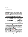
1
User's Manual for the Program Package ECOWEIGHT (C Programs for Calculating Economic Weights in Livestock), Version 5.0.2. Part 3B: Program GFSH for Gene Flow in Sheep, Version 1.0.2 by J. Wolf, M. Wolfová May 14, 2010 1 Authors' addresses: Jochen Wolf and Marie Wolfová, Institute of Animal Science, P.O.Box 1, CZ 10401 Praha Uh°ín¥ves, Czech Republic, E-mail addresses: [email protected] [email protected], wol- Preface The program GFSH together with the program EWSH2 [6] form the third part of the program package ECOWEIGHT. The program GFSH was written within the framework of the research project MZE0002701404 of the Ministry of Agriculture of the Czech Republic starting in the year 2009. Travelling was funded by the Ministries of Education of the Czech Republic and Slovak Republic (Program KONTAKT, project number MEB 080802 or SK-CZ-0007-07). The technical assistance of Renata Pro²ková (Prague-Uh°ín¥ves), Praha U°ín¥ves, is acknowledged. 2 License conditions This program is distributed under the conditions of the GNU GENERAL PUBLIC LICENSE. You will nd the details of the license in the enclosed le license . Please read this le carefully. Especially notice the following part of the license: NO WARRANTY 11. BECAUSE THE PROGRAM IS LICENSED FREE OF CHARGE, THERE IS NO WARRANTY FOR THE PROGRAM, TO THE EXTENT PERMITTED BY APPLICABLE LAW. EXCEPT WHEN OTHERWISE STATED IN WRITING THE COPYRIGHT HOLDERS AND/OR OTHER PARTIES PROVIDE THE PROGRAM "AS IS" WITHOUT WARRANTY OF ANY KIND, EITHER EXPRESSED OR IMPLIED, INCLUDING, BUT NOT LIMITED TO, THE IMPLIED WARRANTIES OF MERCHANTABILITY AND FITNESS FOR A PARTICULAR PURPOSE. THE ENTIRE RISK AS TO THE QUALITY AND PERFORMANCE OF THE PROGRAM IS WITH YOU. SHOULD THE PROGRAM PROVE DEFECTIVE, YOU ASSUME THE COST OF ALL NECESSARY SERVICING, REPAIR OR CORRECTION. 12. IN NO EVENT UNLESS REQUIRED BY APPLICABLE LAW OR AGREED TO IN WRITING WILL ANY COPYRIGHT HOLDER, OR ANY OTHER PARTY WHO MAY MODIFY AND/OR REDISTRIBUTE THE PROGRAM AS PERMITTED ABOVE, BE LIABLE TO YOU FOR DAMAGES, INCLUDING ANY GENERAL, SPECIAL, INCIDENTAL OR CONSEQUENTIAL DAMAGES ARISING OUT OF THE USE OR INABILITY TO USE THE PROGRAM (INCLUDING BUT NOT LIMITED TO LOSS OF DATA OR DATA BEING RENDERED INACCURATE OR LOSSES SUSTAINED BY YOU OR THIRD PARTIES OR A FAILURE OF THE PROGRAM TO OPERATE WITH ANY OTHER PROGRAMS), EVEN IF SUCH HOLDER OR OTHER PARTY HAS BEEN ADVISED OF THE POSSIBILITY OF SUCH DAMAGES. 3 Contents Preface 2 License conditions 3 1 Introduction 6 2 General principles of gene ow 8 3 Pure-bred system 3.1 10 Calculation of the elements of the transmission matrix P. . . . . . . 11 3.2 P11 . . . . . . . . . . . . . . . . . . . . . . . . 3.1.2 Submatrix P12 . . . . . . . . . . . . . . . . . . . . . . . . 3.1.3 Submatrix P21 . . . . . . . . . . . . . . . . . . . . . . . . 3.1.4 Submatrix P22 . . . . . . . . . . . . . . . . . . . . . . . . 3.1.5 Submatrix P31 . . . . . . . . . . . . . . . . . . . . . . . . 3.1.6 Submatrix P32 . . . . . . . . . . . . . . . . . . . . . . . . 3.1.7 Submatrices P13 , P23 and P33 . . . . . . . . . . . . . . Calculation of vectors m (m_gf [∗] in the program), hd and hm . . 13 3.3 Calculation of economic weights . . . . . . . . . . . . . . . . . . . . . 13 3.1.1 Submatrix . . 11 . . 12 . . 12 . . 12 . . 12 . . 12 . . 13 4 Terminal crossing 14 4.1 Calculation of the elements of the transmission matrix 4.2 P11 , P12 , P21 and P22 . . . . 4.1.2 Submatrices P31 and P32 . . . . . . . . . . 4.1.3 Submatrix P33 . . . . . . . . . . . . . . . . 4.1.4 Submatrices P44 and P55 . . . . . . . . . . 4.1.5 Submatrices P45 and P54 . . . . . . . . . . 4.1.6 Submatrices P61 and P62 . . . . . . . . . . 4.1.7 Submatrices P74 and P75 . . . . . . . . . . 4.1.8 Submatrix P83 . . . . . . . . . . . . . . . . 4.1.9 Submatrix P85 . . . . . . . . . . . . . . . . Vectors m (m_gf [∗] in the program), hd and hm 4.3 4.1.1 Submatrices P. . . . . . . 16 . . . . . . . . . . 16 . . . . . . . . . . 16 . . . . . . . . . . 16 . . . . . . . . . . 17 . . . . . . . . . . 17 . . . . . . . . . . 17 . . . . . . . . . . 18 . . . . . . . . . . 18 . . . . . . . . . . 18 Calculation of economic weights . . . . . . . . . . . . . . . . . . . . . 18 5 Relative economic weights 20 6 Installing and running the program 6.1 15 . . . . . . . . . . List of les in the installation package 22 . . . . . . . . . . . . . . . . . 22 6.1.1 Directory PROG . . . . . . . . . . . . . . . . . . . . . . . . . 22 6.1.2 Directory PS1 . . . . . . . . . . . . . . . . . . . . . . . . . . . 23 6.1.3 Directory PS2 . . . . . . . . . . . . . . . . . . . . . . . . . . . 23 6.1.4 Directory DOC . . . . . . . . . . . . . . . . . . . . . . . . . . 24 6.1.5 Directory SRC 24 . . . . . . . . . . . . . . . . . . . . . . . . . . 4 CONTENTS 6.2 6.3 6.4 5 Installation . . . . . . . . . . . . . . . . . . . . . . . . . . . . . . . . Under LINUX . . . . . . . . . . . . . . . . . . . . . . . . . . 24 6.2.2 Under Microsoft Windows . . . . . . . . . . . . . . . . . . . . 24 Running the program . . . . . . . . . . . . . . . . . . . . . . . . . . 7.2 25 6.3.1 Running the program for production system 1 . . . . . . . . 6.3.2 Running the program for production system 2 . . . . . . . . 26 . . . . . . . . . . . . . . . . . . . . . . . . . . . . . 28 General remarks 7 Input les 7.1 24 6.2.1 25 29 Parameter les . . . . . . . . . . . . . . . . . . . . . . . . . . . . . . 29 7.1.1 File P01.TXT . . . . . . . . . . . . . . . . . . . . . . . . . . . 29 7.1.2 File PARAGFS.TXT . . . . . . . . . . . . . . . . . . . . . . . 30 Data input les . . . . . . . . . . . . . . . . . . . . . . . . . . . . . . 30 7.2.1 Input le INPUTGFS01A.TXT . . . . . . . . . . . . . . . . . 30 7.2.2 Input le INPUTGFS01B.TXT . . . . . . . . . . . . . . . . . 30 7.2.3 Input le INPUTGFS02.TXT . . . . . . . . . . . . . . . . . . 31 7.2.4 Input le INPUTGFS03.TXT . . . . . . . . . . . . . . . . . . 31 7.2.5 Input le INPUTGFS04.TXT . . . . . . . . . . . . . . . . . . 33 7.2.6 Input le INPUTGFS05.TXT . . . . . . . . . . . . . . . . . . 33 7.3 TEXTGFS_OUT.TXT . . . . . . . . . . . . . . . . . . . . . . . . . 33 7.4 ERROR.TXT . . . . . . . . . . . . . . . . . . . . . . . . . . . . . . . 33 8 Program output 35 8.1 The results le . . . . . . . . . . . . . . . . . . . . . . . . . . . . . . 35 8.2 File CHECKGFS . . . . . . . . . . . . . . . . . . . . . . . . . . . . . 36 Bibliography 37 A Numbering of traits in the program 38 B List of variables and constants 40 Chapter 1 Introduction The program package ECOWEIGHT is intended for the calculation of economic values of economically important traits in livestock. At the given stage, in its fth version, two programs for cattle and three programs for sheep are available (see Table 1.1). The two programs for cattle (EWBC and EWDC) are described in the rst part of the manual [4]. The second part of the program package is a stand-alone program (EWSH1) for sheep with one lambing per year [5]. Table 1.1: Survey on the program package ECOWEIGHT, version 5.0.2 Part a 01 02 b Installation Package Program(s) ECOWEIGHT01_5_0_2.tgz ECOWEIGHT02_5_0_2.tgz Species, remarks EWBC beef cattle EWDC dairy cattle EWSH1 sheep, one lambing per year, stand-alone program 03A ECOWEIGHT03_5_0_2.tgz EWSH2 for both parts 03A and 03B sheep, one lambing per year, used in combination with GFSH 03B GFSH sheep, program for gene ow, used in combination with EWSH2 a There is one manual for each part; its name is ECOWEIGHT[part].pdf where [part] is to be replaced by the two or three digits given in this column. b Replace 'tgz' by 'zip' for Windows. The third part of the program package which is distributed as one installation package consists of the programs for sheep EWSH2 and GFSH which are documented in two separate manuals. In the present manual, the program GFSH is described which models gene ow in sheep and allows to calculate economic weights for direct and maternal trait components. This program is used in connection with the program EWSH2 [6]. In dependence of the production system, one or more runs of EWSH2 are necessary before GFSH is started. At the beginning of the present manual, a short description of the general principles of gene transfer is given (Chapter 2). The simplest production system which can be modelled is a pure-bred system with one production level where no distinction is made between nucleus and commercial herds. The calculation of economic weights for direct and maternal trait components for this system is described in Chapter 3. Next a production system with terminal crossing is described where also only one production level is assumed (Chapter 4). In this system, two breeds 6 CHAPTER 1. INTRODUCTION 7 are included. A pure-bred system is modelled for sire breed A. In the production system for dam breed B, a part of progeny are pure-bred animals of breed B and another part of progeny are cross-bred animals A×B. That means, the production systems for both breeds are connected via sires from breed A which are crossed to ewes of breed B. Next, relative economic weights are calculated which allow to compare economic weights between traits (Chapter 5). The next chapters deal with technical details of using the program GFSH. First, information on installing and running the program is given (Chapter 6). The following chapter gives a list of the input les needed for running the program and nally the program output is commented (Chapter 8). The Appendix contains a list of traits with their numbering as it was used in the source code of the program and a list of all variables used in the source code of the program. Chapter 2 General principles of gene ow Gene ow methods which were developed by Elsen and Moquot [2] and Hill [3] allow studying the ow of genes through a population, which in turn can be used to dene the times at which genes are expressed, and by knowing the value of that expression and the number of animals involved, the economic value of that expression can be calculated [1]. At any given time t, animals in a population can be divided into a number of dierent sex and age classes. A gene ow diagram can then be constructed to follow the movement of genes through the population over time. Time t is given in reproductive cycles (i.e. years in the case of one lambing per year). A vector m is dened the elements of which dene the proportion of genes acm, the total number n_sac is selected for. th element Then, at time t = 0, all elements of m with the exception of the n_sac th [t] will be zero and the n_sac element of m will be one. Let us write m for m at time t and P for the transmission matrix which is of dimension acm × acm and the elements pij of which are the probability that genes from the sex and age class j [0] are transmitted to the sex and age class i during one time unit. Knowing m (i.e. [t] vector m at the time 0), m is calculated as: in each sex and age class. The dimension of the vector is of sex and age classes. Assume that the sex and age class m[t] = Pm[t−1] = P2 m[t−2] = . . . = Pt m[0] . (2.1) According to Wolfová and Nitter [7] most traits can be considered to belong to one of two groups in animal breeding. The rst group of traits occurs only once in an animal's life (e.g. growth and carcass traits). The second group is realised mostly by females several times in their life (e.g. lactation and fertility traits, but also wool traits). For simplicity we will designate the rst group as direct traits and the second group as maternal traits having in mind that the second group of traits may be exceptionally also expressed in males (wool traits). Some traits (growth of lambs until weaning or conception rate) are composite traits with a direct and a maternal genetic component, the direct component realized once by the ospring and the maternal component realized several times during the female's life. For the calculation of the number of discounted expressions, we need so-called realization vectors, hd and hm , for direct and maternal eects, respectively. A realization vector describes the extend of the expression of a trait in the individual sex and age classes. Therefore, both realization vectors are of dimension acm. Examples for realization vectors are given in the following chapters. Out of the analyzed traits (see Appendix A), the following ones are considered to be direct traits: growth rates in articial rearing, in fattening and in rearing of breeding animals, survival rates in articial rearing and all carcass traits, (traits 8 CHAPTER 2. GENERAL PRINCIPLES OF GENE FLOW 4 to 7, 9 to 19 and 25). 9 On the other hand, mature weight, milk yield, fat and protein content or yield, somatic cell count, average litter size, wool production and productive life of ewes are considered to be maternal traits (traits 8, 22 and 26 to 35). Mature weight is considered as maternal trait because there are maintenance costs in each reproductive cycle. Wool is repeatedly sheared. Productive lifetime may be understood as a result of successive surviving in the individual reproductive cycles. Several traits have direct and maternal components: birth weight, weaning weight, growth rate from birth till weaning, survival rate of lambs at birth and until weaning and conception rate (traits 1 to 3, 20, 21, 23 and 24). The direct component of growth traits till weaning expresses the genetic potential of lambs for growth, the maternal component expresses the genetic potential of the dam for milk available to lambs. The direct eect of the lamb survival rate expresses the health status of the lambs, the maternal eect is determined by the mothering ability of a 1 ewe . 1 Maternal components of growth traits and survival rates till weaning will therefore be expressed both on pure-bred and on cross-bred progeny. Chapter 3 Production system 1: Pure-bred system with one production level In this system, the population of sheep is not distinguished in nucleus and commercial herds. The system is similar as in cattle, where the dams of sires are selected from the whole population (see Fig. 3.1). Only one breed is considered in this production system and the capital letter A is used to designate this breed; this letter is used at the end of several variables to make clear that these variables refer to breed A. 1 is calculated as The number of age classes for sires (acsA) acsA = int ageR11A 365 + RRA (3.1) and the number of age classes for dams (acdA) is acdA = int + LLA . (3.2) Pure−bred population female replacement variables are explained in Appendix B male replacement 1 All ageE1A 365 Slaughter animals Figure 3.1: Pure-bred system with one production level 10 CHAPTER 3. PURE-BRED SYSTEM Algorithm 3.1 Structure of matrix 11 P. The symbol x characterizes elements which can be dierent from zero (The values of x are in the range from 0 to 0.5). Slaughter Sires P= x x x 1 0 0 0 1 0 0 0 1 0 0 0 0 0 0 x x x 0 0 0 0 0 0 0 0 0 0 0 0 0 0 0 x x x ··· ··· ··· ··· Dams x x x x x 0 0 0 0 0 0 0 0 0 0 0 0 0 0 0 0 1 0 0 0 0 0 0 0 0 x x x x x 0 0 0 0 0 0 1 0 0 0 1 0 0 0 1 ··· 0 0 0 0 0 0 0 0 0 0 ··· x x x x x .. . ··· ··· ··· ··· ··· .. . The dimension of the transmission matrix animals ··· ··· ··· ··· x x 0 0 0 0 0 0 0 0 0 0 0 0 0 0 0 0 x x 0 0 0 0 0 0 0 0 0 0 ··· 0 1 0 0 0 0 ··· x x 0 .. . ··· ··· ··· ··· ··· .. P . Sires Dams Slaughter animals for gene ow (acm) is then acm = acsA + acdA + 1 . (3.3) 3.1 Calculation of the elements of the transmission matrix P Matrix P has a block structure containing 3×3 blocks (see Algorithm 3.1). There- fore we can write matrix P in the form: P11 P = P21 P31 The elements at time t elements P [i][j] of P P12 P22 P32 P13 P23 P33 i t − 1. The sum of all elements P [i][j] within each are the proportions of genes in the sex and age class which come from the sex and age class P [i][j] (3.4) j at time within each row is 1. The sum of all row belonging to the same sex is 0.5 if there are non-zero elements for both sexes in this row. This is the case when vertically new blocks start (see Algorithm 3.1). For calculating the elements P [i][j] (i, j = 1, . . . , acm) of P, rst all elements are set to zero. Then the non-zero elements are inserted as given below. 3.1.1 Submatrix P11 P11 is the sires-to-sires part of the transmission matrix and is of diacsA × acsA. The elements of the rst row may be read in from input le Submatrix mension INPUTGFS02.TXT if the sires for the production of rams are selected from certain age classes. If there is no selection among sires of rams, the elements in the rst row are calculated as follows: P [1][acsA − RRA + i] = 0.5 × l4RA[i] where i = 1, . . . , RRA . (3.5) CHAPTER 3. PURE-BRED SYSTEM 12 The further elements dierent from zero are: P [i + 1][i] = 1 i = 1, . . . , acsA − 1 for . (3.6) The diagonal of elements 1 describes aging of animals of the given group. 3.1.2 Submatrix P12 P12 is the dams-to-sires part of the transmission matrix and is of acsA × acdA. The elements of the rst row may be read in from input The submatrix dimension le INPUTGFS02.TXT if the dams for the production of rams are selected from certain age classes. If there is no selection among dams of rams, the elements in the rst row are calculated as follows: P [1][acsA + acdA − LLA + i] = 0.5 × l4EA[i] where i = 1, . . . , LLA . (3.7) These are the only elements dierent from zero in this submatrix. 3.1.3 Submatrix P21 P21 is the sires-to-dams acdA × acsA. The elements of The submatrix part of the transmission matrix and is of dimension its rst row are: P [acsA + 1][acsA − RRA + i] = 0.5 × l4RA[i] where i = 1, . . . , RRA . (3.8) These are the only elements dierent from zero in this submatrix. 3.1.4 Submatrix P22 P22 is the dams-to-dams part of the transmission acdA × acdA. The elements of its rst row are: The submatrix of dimension P [acsA + 1][acsA + acdA − LLA + i] = 0.5 × l4EA[i] where matrix and is i = 1, . . . , LLA . (3.9) The further elements dierent from zero are: P [acsA + i + 1][acsA + i] = 1 for i = 1, . . . , acdA − 1 . (3.10) The diagonal of elements 1 again describes aging of animals of the given group. 3.1.5 Submatrix P31 The submatrix P31 is the sires-to-slaughter animals part of the transmission ma- trix and is of dimension 1 × acsA. The elements of its only row are the same as the elements in the rst row of submatrix P21 : P [acm][acsA − RRA + i] = 0.5 × l4RA[i] where i = 1, . . . , RRA . (3.11) 3.1.6 Submatrix P32 The submatrix P32 is the dams-to-slaughter animals part of the transmission matrix and is of dimension 1 × acdA. The elements of its only row are the same as the elements in the rst row of submatrix P31 : P [acm][acsA + acdA − LLA + i] = 0.5 × l4EA[i] where i = 1, . . . , LLA . (3.12) CHAPTER 3. PURE-BRED SYSTEM 13 3.1.7 Submatrices P13 , P23 and P33 The matrices P13 , P23 and P33 are the slaughter animals to sires, slaughter animals to dams and slaughter animals to slaughter animals parts, respectively, of the transmission matrix. The dimension of these matrices is and 1 × 1. 1 × acsA, 1 × acdA As no genes are transmitted from slaughter animals, all elements of these submatrices are zero. 3.2 Calculation of vectors m (m_gf [∗] in the program), hd and hm 2 n_sac, the number of the sex and age class the selection is carried out m[0] from equation (2.1), all elements of the vector m_gf [∗] are set to [t] zero and m_gf [n_sac] = 1. Then equation (2.1) is applied to calculate m . The l_inv X expression m[t] (1 + u)−t is calculated as vector m_sum[∗] in the program. Given is for. To get t=1 The notations h_d[∗] last element of the vector h_m[∗] are h_d[∗] is one: and hd used in the program for and hm . h_d[acm] = 1 (3.13) and all remaining elements of the vector are zero. The rst last element of acdA − LLA h_m[∗] are zero if are zero. The acsA elements and the acsA + 1 to acsA + Furthermore the elements acdA > LLA. The remaining elements are: h_m[acsA + acdA − LLA + i] = l4EA[i] i = 1, . . . , LLA for . (3.14) 3.3 Calculation of economic weights The economic weights for direct eects (ew _d[i]) and for maternal eects (ew _m[i]) of trait i are calculated as follows: ew_d[i] ew_m[i] = evp[i][1] × = evp[i][1] × acm X i=1 acm X h_d[i] × m_sum[i] h_m[i] × m_sum[i] if tt[i] = 0 if or tt[i] = 1 tt[i] = 2 or tt[i] = 2 . i=1 (3.15) 2 In most cases the same symbols for variables are used in the manual and in the program written in C. For dierentiating between a vector or a matrix (generally an array) and its elements, we use an index i, j, k etc. for an element of the array and use the symbol '*' instead of an index to refer to the array as such. Chapter 4 Production system 2: System with terminal crossing and one production level only In this production system, specialized sire and dam breeds are assumed. Sire and dam breed ocks are assumed to be self-replacing producing both males and females for own replacement (selling and purchasing of breeding animals between farms within each breed is not taken into account in the prot function for the calculation of economic values). Sire breed ocks produce also sires for terminal crossing in the dam breed ocks (see Figure 4.1). The number of age classes for sires of breed A used for pure-breeding (acsA) and the number of age classes for dams of breed A (acdA) are calculated according to equations (3.1) and (3.2), respectively. The age classes for sires of breed B (acsB ) and the number of age classes for dams of breed B (acdB ) are calculated in the same way as the corresponding variables for breed A (replace A by B in equations (3.1) and (3.2)). The number of age classes for sires of breed A used for cross-breeding 1 with ewes of breed B (acsAB ) is : acsAB = int ageR12A 365 + RRB . (4.1) The total number of sex and age classes which is identical with the dimension 1 The same age structure and the same number of breeding cycles is assumed for rams of breeds A and B in the ock of breed B. sires A Dam breed B slaughter animals AxB female replacement B Partly terminal crossing Sire breed A male replacement B female replacement male replacement slaughter animals A slaughter animals B Figure 4.1: System with terminal crossing on one production level 14 CHAPTER 4. TERMINAL CROSSING of the transmission matrix P 15 for gene ow (acm) is then acm = acsA + acdA + acsAB + acsB + acdB + 3 . (4.2) 4.1 Calculation of the elements of the transmission matrix P Matrix P has a block structure containing 8×8 blocks and can be therefore written as: P11 P21 P= . .. P81 P12 P22 ··· ··· . . . .. P82 ··· . P18 P28 . . . P88 (4.3) This structure is the consequence of the following 8 groups of sex and age classes (in parentheses the number of classes is given): • Age classes for sires of breed A used for pure-breeding (acsA) • Age classes for dams of breed A (acdA) • Age classes for sires of breed A used for crossing with ewes of breed B (acsAB ) • Age classes for sires of breed B (acsB ) • Age classes for dams of breed B (acdB ) • Age class for slaughter animals of breed A (1) • Age class for slaughter animals of breed B (1) • Age class for slaughter animal A×B (1) All submatrices of S1 to S4 P with non-zero elements have one of the following structures (the symbol x characterizes elements which may be dierent from zero): S1 = S2 = S3 = S4 = x x x 1 0 0 0 1 0 0 0 1 0 0 0 0 0 0 x x x 0 0 0 0 0 0 0 0 0 ··· ··· ··· ··· .. . ··· ··· ··· ··· ··· .. . x x 0 0 0 0 0 0 0 1 x 0 0 0 0 0 0 0 0 0 0 ··· 0 0 x x x ··· x 0 1 0 0 0 0 1 0 0 0 0 1 0 0 0 0 0 0 ··· ··· ··· ··· .. . ··· 0 0 x 0 0 0 0 0 0 0 1 0 0 x 0 0 0 0 (4.4) (4.5) (4.6) 0 0 (4.7) CHAPTER 4. TERMINAL CROSSING 16 4.1.1 Submatrices P11 , P12 , P21 and P22 The elements of submatrices P11 , P12 , P21 P22 and are calculated in the same way as in production system 1 (subsections 3.1.1 to 3.1.4, equations 3.5 to 3.10) so that submatrices P21 P12 P11 P22 are of the structure S1 and submatrices P12 S2 . The elements of the rst rows of submatrices P11 and are of the structure and and may be read in from input le INPUTGFS03.TXT. 4.1.2 Submatrices P31 and P32 Submatrices P31 and P32 are of the structure S2 . P31 represents the gene ow from sires of breed A used for pure-breeding to sires of breed A used for cross-breeding and P32 represents the gene ow from dams of breed A to sires of breed A used for cross-breeding. P31 and P32 are of dimension respectively. The non-zero elements of P31 acsAB × acsA P [acsA + acdA + 1][i] = P [1][i] P32 acsAB × acdA, i = 1, . . . , acsA for i.e. they are the same as the elements in the rst row of of and are: P11 . , (4.8) The non-zero elements are: P [acsA + acdA + 1][acsA + i] = P [1][acsA + i] i = 1, . . . , acdA for i.e. they are the same as the elements in the rst row of , (4.9) P12 . 4.1.3 Submatrix P33 P33 is the sires to sires matrix for sires of breed A used for cross-breeding with dams of breed B. It is of type S4 . Consequently, its non-zero elements are: P [acsA + acdA + i + 1][acsA + acdA + i] = 1 for i = 1, . . . , acsAB − 1 . (4.10) 4.1.4 Submatrices P44 and P55 P44 is the sires to sires matrix for breed B and for breed B. Both matrices are of type S1 . P55 is the dams to dams matrix The elements of the rst row of P44 may be read in from input le INPUTGFS03.TXT if the sires of breed B for the production of rams are selected from certain age classes. Otherwise the elements of the rst row of P44 are calculated as follows: P [acsA + acdA + acsAB + 1][acsA + acdA + acsAB + acsB − RRB + i] 0.5 × l4RB[i] for i = 1, . . . , RRB . The remaining non-zero elements of P44 = (4.11) are: P [acsA+acdA+acsAB+i+1][acsA+acdA+acsAB+i] = 1 for i = 1, . . . , acsB−1 . (4.12) The elements of the rst row of P55 are: P [j][k] = 0.5 × l4EB[i] for i = 1, . . . , LLB (4.13) where j = acsA + acdA + acsAB + acsB + 1 and k = acsA + acdA + acsAB + acsB + acdB − LLB + i The further non-zero elements of P55 . are: P [acm − acdB − 2 + i][acm − acdB − 3 + i] = 1 for i = 1, . . . , acdB − 1 . (4.14) CHAPTER 4. TERMINAL CROSSING 17 4.1.5 Submatrices P45 and P54 P45 is the dams to sires matrix for breed B and for breed B. Both matrices are of type S2 . P54 is the sires to dams matrix The elements of the rst row of P45 may be read in from input le INPUTGFS03.TXT if the dams for the production of rams are selected from certain age classes. Otherwise the non-zero elements of matrix P45 are calculated in the program: P [j][k] = 0.5 × l4EB[i] i = 1, . . . , LLB for (4.15) where j = acsA + acdA + acsAB + 1 and k = acsA + acdA + acsAB + acsB + acdB − LLB + i The elements of the rst row of P54 . are calculated as: P [j][k] = 0.5 × l4RB[i] for i = 1, . . . , RRB (4.16) where j = acsA + acdA + acsAB + acsB + 1 and k = acsA + acdA + acsAB + acsB − RRB + i . 4.1.6 Submatrices P61 and P62 P61 P62 is the sires A to slaughter animals A matrix and animals A matrix. Both matrices are of type S3 . P [acm − 2][acsA − RRA + i] = 0.5 × l4RA[i] and the elements of matrix P62 for P21 and the elements of P61 P62 P61 i = 1, . . . , RRA are: (4.17) are: P [acm − 2][acsA + acdA − LLA + i] = 0.5 × l4EA[i] That means the elements of is the dams A to slaughter The elements of matrix for i = 1, . . . , LLA . (4.18) are the same as the elements in the rst row of are the same as the elements in the rst row of P22 . 4.1.7 Submatrices P74 and P75 P74 is the sires B to slaughter animals B matrix and animals B matrix. Both matrices are of type S3 . P75 is the dams B to slaughter The elements of matrix P [acm − 1][acsA + acdA + acsAB + acsB − RRB + i] for and the elements of matrix P [j][k] = 0.5 × l4EB[i] × = P74 0.5 × l4RB[i] i = 1, . . . , RRB P75 (4.19) are: 1 − pcrossE[i − 1] LLB X for i = 1, . . . , LLB (1 − pcrossE[l − 1]) l=1 where j = acm − 1 and k = acsA + acdA + acsAB + acsB + acdB − LLB + i The elements of P74 are: . are the same as the elements in the rst row of P54 . (4.20) CHAPTER 4. TERMINAL CROSSING 18 4.1.8 Submatrix P83 P83 is the sires A to cross-bred slaughter animals matrix. It is of type S3 . Its elements are: P [acm][acsA + acdA + acsAB − RRB + i] = 0.5 × l4RB[i] for i = 1, . . . , RRB . (4.21) 4.1.9 Submatrix P85 P85 is the dams B to cross-bred slaughter animals matrix. It is of type S3 . Its elements are: P [j][k] = 0.5 × l4EB[i] × pcrossE[i − 1] LLB X i = 1, . . . , LLB for (4.22) pcrossE[l − 1] l=1 where j = acm and k = acsA + acdA + acsAB + acsB + acdB − LLB + i . 4.2 Vectors m (m_gf [∗] in the program), hd and hm Vectors m_gf [∗] and m_sum[∗] are calculated in the same way as in production system 1 (see section 3.2 on page 13). They are of dimension subdivided into 8 blocks in the same way as matrix Also vectors vector h_d[∗], h_d[∗] and h_m[∗] acm and can be P. are of dimension acm and have 8 blocks. In only the elements referring to slaughter animals are dierent from zero: h_d[acm − 2] = pdA, In the vector for maternal eects, h_d[acm − 1] = h_d[acm] = pdB (4.23) h_m[∗], non-zero elements are in the blocks dams A and dams B: h_m[acsA + acdA − LLA + i] = l4EA[i] × pdA for i = 1, . . . , LLA h_m[acm − 3 − LLB + i] = l4EB[i] × pdB for i = 1, . . . , LLB (4.24) The elements of the vector hm sum to 1. 4.3 Calculation of economic weights h_d[∗] and h_m[∗] with the marginal economic values he_d[∗][∗] and he_m[∗][∗] are calculated. The rst index By multiplying the vectors of each trait, the matrices of the matrices refers to the number of the trait and the second index refers to the sex and age class. are set zero. First, all elements of the matrices The non-zero elements of he_d[∗][∗] he_d[∗][∗] and he_m[∗][∗] are calculated as follows (for i = 1, . . . , N T − 1): he_d[i][acm − 2] = h_d[acm − 2] × evpA[i][1] he_d[i][acm − 1] = h_d[acm − 1] × evpB[i][1] he_d[i][acm] = h_d[acm] × evpB[i][2] (4.25) CHAPTER 4. TERMINAL CROSSING 19 Table 4.1: Values of a (i) Number of the trait tt[i] Value of 4 to 7, 9 to 19, 20, 25 tt[i] 0 8, 22, 26 to 35 1 1 to 3, 21, 23, 24 2 a See Appendix A for numbering traits The non-zero elements of he_m[∗][∗] are (for i = 1, . . . , N T − 1): he_m[i][j] = h_m[j] × evpA[i][1] he_m[i][j] = h_m[j] × (evpB[i][1] + evpB[i][2]) for for j = acsA + 1, . . . , acsA + acdA (4.26) j = acm − acdB − 2, . . . , acm − 3 The economic weights for the direct and the maternal components of trait ew_d[i] and ew_m[i], ew_d[i] ew_m[i] = = i, are calculated as follows: acm X j=1 acm X he_d[i][j] × m_sum[j] he_m[i][j] × m_sum[j] if tt[i] = 0 if or tt[i] = 1 tt[i] = 2 or tt[i] = 2 (4.27) j=1 where 0 1 tt[i] = 2 The values of if there is only a direct component of trait i if there is only a maternal component of trait i if there are both a direct and a maternal component of trait tt[i] are xed in the program (see Table 4.1). i These economic weights are valid for the sex and age class of animals which is determined by the variable n_sac. The economic weight of trait i or component of trait i represents the present value (in monetary units) of one unit genetic superiority of the selected group of animals in this trait transmitted in the evaluated production (breeding) system during the dened investment period per ewe in this production system. If the economic weights are calculated for breed A they can be easily converted to be per ewe of breed A by dividing the weights calculated by equation (4.27) by the proportion of ewes of breed A in the production system (pdA). Similarly, the economic weights per ewe of breed B may be calculated by dividing the weights from equation (4.27) by the proportion of ewes of breed B in the production system (pdB ). Chapter 5 Relative economic weights The economic weights of the individual traits as they are calculated in sections 3.3 and 4.3 cannot be compared among each other as they have dierent units. One way to make the economic weights comparable is to refer them to the genetic standard deviation of the trait. These so-called standardized economic weights for the direct and the maternal trait components (ewst_d[i] and ewst_d[i] ewst_m[i] where gstd_d[i] and gstd_m[i] ewst_m[i]) are calculated as: = ew_d[i] × gstd_d[i] = ew_m[i] × gstd_m[i] (5.1) are the genetic standard deviations for the direct and maternal components of trait i (i = 1, . . . , N T − 1).The standardized economic weights are given in monetary units per standard deviation of the trait component and per ewe in the whole production system. As the standardized economic weights have the same units for all traits, they can be expressed as percentage of the sum of all standardized economic weights. When calculating the sum, care must be taken of not including the same trait twice. Therefore, in input le INPUTGFS05.TXT (see Subsection 7.2.6) you must choose always one trait denition from two alternatives for six paires of denitions describing always the same trait in dierent ways. As both positive and negative values occur it is useful to calculate the sum from the absolute values of the economic weights. It may be useful to calculate this sum for the economic weights of the direct components of the traits (ewsum_d), for the economic weights of the maternal components of the traits (ewsum_m) and for both components together (ewsum): ewsum_d = NX T −1 delta_d[i] × abs(ewst_d[i]) i=1 ewsum_m = NX T −1 delta_m[i] × abs(ewst_m[i]) (5.2) i=1 and ewsum = ewsum_d + ewsum_m The variables delta_d[i] and delta_m[i] . (5.3) take only values 1 or 0 depending on con- sidering or not considering the corresponding trait. The following proportions of standardized economic weights (which are called relative economic weights) may be calculated: 20 CHAPTER 5. • RELATIVE ECONOMIC WEIGHTS Standardized economic weight for the direct component of trait 21 i expressed as percentage of the sum of all standardized economic weights for the direct components: ewr_dd[i] = 100 × • abs(ewst_d[i]) (5.4) ewsum_d Standardized economic weight for the direct component of trait i expressed as percentage of the sum of all standardized economic weights for both the direct and the maternal components: ewr_da[i] = 100 × • abs(ewst_d[i]) ewsum Standardized economic weight for the maternal component of trait (5.5) i expressed as percentage of the sum of all standardized economic weights for the maternal components: ewr_mm[i] = 100 × • abs(ewst_m[i]) ewsum_m Standardized economic weight for the maternal component of trait (5.6) i expressed as percentage of the sum of all standardized economic weights for both the direct and the maternal components: ewr_ma[i] = 100 × abs(ewst_m[i]) ewsum (5.7) Chapter 6 Installing and running the program 6.1 List of les in the installation package The program GFSH is distributed together with the program EWSH2 [6]. Therefore, les for both programs are in the installation package. The les are in ve directories. 6.1.1 Directory PROG This directory contains executable program les and text les which are not to be edited. ewsh2.exe gfsh.exe Executable le for program EWSH2 [6]. Executable le for program GFSH. TEXTS2_OUT.TXT This le contains text for writing the results for the pro- gram EWSH2. For further details see the manual for the program EWSH2 [6]. TEXTGFS_OUT.TXT This le contains text for writing the results for the program GFSH. See also Section 7.3. P01_00.TXT (prods This le contains the initial parameters for the production system = 1), the breed (breed = 1) and the number of the run of EWSH2 (calc = 1) for production system 1. P02_00.TXT (prods This le contains the initial parameters for the production system = 2), the breed (breed = 2) and the number of the run of EWSH2 (calc = 1) for production system 2. ERROR.TXT A text le forwarding error messages between succesive runs of the program EWSH2 and the program GFSH. The le in this directory contains the starting value 0 which means no error message. cygwin1.dll This is a le from Cygwin which is necessary for running the pro- grams under Windows. It is contained only in the distribution for Windows. 22 CHAPTER 6. INSTALLING AND RUNNING THE PROGRAM 23 6.1.2 Directory PS1 This directory contains les necessary for running production system 1. Production system 1 is only for one breed. Without loss of generality, we will call this breed A. PARASA.TXT Parameter le which contains the most important parameters for running the program EWSH2. For further details see the manual for the program EWSH2 [6]. PARAGFS.TXT Parameter le which contains the most important parameters for running the program GFSH (see Section 7.1.2). INPUTS#A.TXT with # = 01, 02, ..., 14 Data input les for program EWSH2. Not all data input les are needed for all calculations. For further details see the manual for the program EWSH2 [6]. INPUTGFS#.TXT with # = 01A, 02, 04 Data input les for program GFSH (see Section 7.2). ps1A.sh under LINUX or ps1A.bat under Windows This is the shell script (LINUX) or batch le (Windows) which starts the calculations for production system 1. 6.1.3 Directory PS2 This directory contains les necessary for running production system 2. This is a system with terminal crossing. There are two breeds. Breed A is the sire breed and breed B is the dam breed. PARASA.TXT, PARASB.TXT Parameter les for breeds A and B, respec- tively, which contain the most important parameters for running the program EWSH2 for the given breed. For further details see the manual for the program EWSH2 [6]. PARAGFS.TXT Parameter le which contains the most important parameters for running the program GFSH (see Section 7.1.2). INPUTS#A.TXT and INPUTS#B.TXT with # = 01, 02, ..., 14 input les for breeds A and B, respectively, for program EWSH2. Data Not all data input les are needed for all calculations. For further details see the manual for the program EWSH2 [6]. INPUTGFS#.TXT with # = 01A, 01B, 03, 04 Data input les for program GFSH (see Section 7.2). ps2AB.sh under LINUX or ps2AB.bat under Windows This is the shell script (LINUX) or batch le (Windows) which starts the calculations for production system 2. CHAPTER 6. INSTALLING AND RUNNING THE PROGRAM 24 6.1.4 Directory DOC license This le contains the license conditions. Read them carefully and do not use the program package ECOWEIGHT if you do not agree with the license conditions. ECOWEIGHT03A.pdf Part 3A of the documentation of the program package ECOWEIGHT, manual for the program EWSH2. ECOWEIGHT03B.pdf Part 3B of the documentation of the program package ECOWEIGHT, manual for the program GFSH. 6.1.5 Directory SRC This directory contains the source les in C language. ewsh2.c gfsh.c Source code of the program EWSH2. Source code of the program GFSH. 6.2 Installation 6.2.1 Under LINUX The program GFSH together with the program EWSH2 come to you as a compressed tar-le with the name ECOWEIGHT03_{# of version}.tgz, for example ECOWEIGHT03_5_0_2.tgz contains the programs from version 5.0.2 of the program package. Copy this le to a directory of your choice and enter the command tar xvf ECOWEIGHT03_{# of version}.tgz for uncompressing and unarchiving the le. You will get the le structure as described in Section 6.1. Only for experts in programming. If you want to do changes in the program (source code) by yourself, then you must use the option -lm for compiling the source code when using the compiler gcc because otherwise the mathematical functions would not work; e.g. gcc -lm -o gfsh.exe gfsh.c will compile the source le gfsh.c to the executable le gfsh.exe. 6.2.2 Under Microsoft Windows The Windows version of the program is distributed as zip le with the name ewsh2.exe gfsh.exe. The programs were compiled under Cygwin (http:// www.cygwin.com) and run only in the presence of the le cygwin1.dll which is part of the Windows ECOWEIGHT03_{# of version}.zip. It contains the compiled programs and distribution. Only for experts in programming. If you intend to change the source code and to compile the program you are recommended to install Cygwin which is freely available. When compiling the source code, the following statement works for the program EWSH2: gcc -Wl,stack=55000000 -o ewsh2.exe ewsh2.c The program GFSH can be simply compiled by the statement CHAPTER 6. INSTALLING AND RUNNING THE PROGRAM 25 gcc -o gfsh.exe gfsh1.c Alternatively it should be possible to use commercial C compilers (we did not test commercial compilers). 6.3 Running the program You are recommended to create one directory for each calculation where you will copy and edit all les you will need. The program may be also in this directory or may be copied to a directory for executable les, e.g. to the directory /usr/local/bin in LINUX. 6.3.1 Running the program for production system 1 All les needed for running production system 1 are in the directory PS1. Furthermore, the directory PROG is needed where the program les and further les are located which should not be edited. The directories PS2, DOC and SRC are not needed for the calculation. Edit the parameter les PARASA.TXT and PARAGFS.TXT and the input les INPUTS#A.TXT with # = 01, 02, ..., 14 and INPUTGFS#.TXT with # = 01A, 02, 04 in directory PS1. Under LINUX, type ./ps1A.sh and press ENTER to start the shell script which runs the programs EWSH2 and GFSH. Under Windows, type ps1A.bat and press ENTER to start the batch le which runs the programs EWSH2 and GFSH. For redirecting the text written to the screen to a text le, say a.txt, type ./ps1A.sh > a.txt ENTER. The shell script under LINUX or ps1A.bat > a.txt under Windows and press ps1A.sh for running production system 1 looks like that: #!/bin/sh echo '*********************************' echo I am copying P01_00.TXT to P00.TXT echo '*********************************' cp ../PROG/P01_00.TXT P00.TXT echo ' ' echo '***************************************************' echo 'I am copying TEXT*_OUT.TXT to the working directory' echo '***************************************************' cp ../PROG/TEXTS2_OUT.TXT . cp ../PROG/TEXTGFS_OUT.TXT . echo ' ' echo '***********************************************' echo 'I am copying ERROR.TXT to the working directory' echo '***********************************************' cp ../PROG/ERROR.TXT . echo ' ' echo '***************************' echo I am starting program EWSH2 echo '***************************' ./../PROG/ewsh2.exe echo ' ' echo '**************************' echo I am starting program GFSH echo '**************************' CHAPTER 6. INSTALLING AND RUNNING THE PROGRAM 26 ./../PROG/gfsh.exe echo ' ' echo '**********' echo I am ready echo '**********' The following two results les will printed: • • resA01 : This is the results le from program EWSH2. resgfps01 : This is the results le from program GFSH described in this manual. Furthermore, the values of all variables are printed for both programs in the following les: • CHECKSA01 : Complete list of the values of all variables of breed A from program EWSH2 at the end of the calculation. The description of the variables is given in Appendix B in the manual for EWSH2 [6]. • CHECKSA01a : Complete list of the values of all variables of breed A from program EWSH2 before the program starts the calculation of economic values. This le is printed mainly as help for further programming and as a check for correct computing. With one exception (variable zr, number of the loop), the values of all variables contained in both les must be equal. The le CHECKSA01a does not contain the economic values which are printed only in CHECKSA01. • CHECKGFS : Complete list of the values of all variables from program GFSH. The description of the variables is given in Appendix B of the present manual. 6.3.2 Running the program for production system 2 All les needed for running production system 2 are in the directory PS2. Furthermore, the directory PROG is needed where the program les and further les are located which should not be edited. The directories PS1, DOC and SRC are not needed for the calculation. Edit the parameter les PARASA.TXT, PARASB.TXT and PARAGFS.TXT and the input les INPUTS#A.TXT with # = 01, 02, ..., 14, INPUTS#B.TXT with # = 01, 02, ..., 14 and INPUTGFS#.TXT with # = 01A, 01B, 03, 04 in ./ps2AB.sh and press ENTER to start the GFSH. Under Windows, type ps2AB.bat and press ENTER to start the batch le directory PS2. Under LINUX, type shell script which runs several times the program EWSH2 and then the program which runs the programs EWSH2 and GFSH. For redirecting the text written to the screen to a text le, say a.txt, type ./ps2AB.sh > a.txt under LINUX or ps2AB.bat > a.txt under Windows and press ENTER. The shell script ps2AB.sh for running production system 2 has the following structure: #!/bin/sh echo '**********************************' echo I am copying P02_00.TXT to P00.TXT echo '**********************************' cp ../PROG/P02_00.TXT P00.TXT echo ' ' CHAPTER 6. INSTALLING AND RUNNING THE PROGRAM 27 echo '***************************************************' echo 'I am copying TEXT*_OUT.TXT to the working directory' echo '***************************************************' cp ../PROG/TEXTS2_OUT.TXT . cp ../PROG/TEXTGFS_OUT.TXT . echo ' ' echo '***********************************************' echo 'I am copying ERROR.TXT to the working directory' echo '***********************************************' cp ../PROG/ERROR.TXT . echo ' ' echo '************************************' echo I am starting program EWSH2, breed B echo '************************************' ./../PROG/ewsh2.exe echo ' ' echo '************************************' echo I am starting program EWSH2, breed A echo '************************************' ./../PROG/ewsh2.exe echo ' ' echo '************************************' echo I am starting program EWSH2, breed A echo '************************************' ./../PROG/ewsh2.exe echo ' ' echo '************************************' echo I am starting program EWSH2, breed B echo '************************************' ./../PROG/ewsh2.exe echo ' ' echo '**************************' echo I am starting program GFSH echo '**************************' ./../PROG/gfsh.exe echo ' ' echo '**********' echo I am ready echo '**********' The following results les will printed: • resB01 : This is the results le from the rst run of program EWSH2 which is for breed B. • resA02 : This is the results le from the second run of program EWSH2 which is for breed A. • resA03 1 : This is the results le from the third run of program EWSH2 which is for breed A. • resB0 42 : This is the results le from the forth run of program EWSH2 which 1 This le contains the nal results for breed A from the program EWSH as the third run of EWSH is the last run for breed A. 2 This le contains the nal results for breed B from the program EWSH2 as the forth run of EWSH2 is the last run for breed B. CHAPTER 6. INSTALLING AND RUNNING THE PROGRAM 28 is for breed B. • resgfps02 : This is the results le from program GFSH described in this manual. Furthermore, the values of all variables are printed for both programs in the following les: • CHECKSB01 : Complete list of the values of all variables of breed B from the rst run of program EWSH2 at the end of the calculation. The description of the variables is given in Appendix B in the manual for EWSH2 [6]. • CHECKSB01a : Complete list of the values of all variables of breed B from the rst run of program EWSH2 before the program starts the calculation of economic values. This le is printed mainly as help for further programming and as a check for correct computing. With one exception (variable zr, number of the loop), the values of all variables contained in both les must be equal. The le CHECKSB01a does not contain the economic values which are printed only in CHECKSB01. • CHECKSA02 : Complete list of the values of all variables of breed A from the second run of program EWSH2 at the end of the calculation. • CHECKSA02a : Complete list of the values of all variables of breed A from the second run of program EWSH2 before the program starts the calculation of economic values. • CHECKSA0 33 : Complete list of the values of all variables of breed A from CHECKSA03a : Complete list of the values of all variables of breed A from the third run of program EWSH2 at the end of the calculation. • the third run of program EWSH2 before the program starts the calculation of economic values. • CHECKSB04 4 : Complete list of the values of all variables of breed B from CHECKSB04a : Complete list of the values of all variables of breed B from the forth run of program EWSH2 at the end of the calculation. • the forth run of program EWSH2 before the program starts the calculation of economic values. • CHECKGFS : Complete list of the values of all variables from program GFSH. The description of the variables is given in Appendix B of the present manual. 6.4 General remarks Several checks of input parameters are included in the programs. For example, certain input parameters have to sum to one. A warning will appear if these input parameters are invalid and the program will stop. You will be told which input parameters to correct before restarting the program. In general, it is your responsibility to use input parameters which are realistic and t together, because it is impossible to predict any possible erroneous combinations of input parameters. Do not forget to have always a critical look on your results before using them for further purposes. 3 See 4 See footnote 1 on the previous page. footnote 2 on the preceding page. Chapter 7 Input les Important remark: quotation marks. When editing the input les, keep attention not to change All les are read as sequential les and the program rec- ognizes the beginning and the end of texts on the basis of quotation marks. Adding or deleting a quotation mark will cause the program to break down or to calculate wrong results. Monetary unit: In all input les the abbreviation MU is used for monetary unit. All values in the distributed version of the program refer to Euros. You can globally replace the abbreviation MU by the abbreviation of your monetary unit in all data input les (INPUTGFS#.TXT) with # = 01A, 01B, 02, 03, 04 and in the input le TEXTGFS_OUT.TXT (which is located in the directory PROG) using any text editor; the results le(s) will then contain the monetary unit specied by you. Language of the program: The program will need just the numbers for calcu- lations. The texts are read in and printed out to the result le as they are. Therefore, you can freely change the text in all input les as long as you do not modify the quotation marks. For example, you can translate all texts in the input les to another language what will cause the appropriate part of the result le to be printed in the same language as the input les (may be there are some exceptions where the English text will be remained). The length of the texts can be changed, but each text must start and nish with quotation marks. A great part of the text for the results le(s) is read from the le TEXTGFS_OUT.TXT (which is located in the directory PROG). You can translate all the text in this le. But be very careful not to change quotation marks. 7.1 Parameter les 7.1.1 File P01.TXT The le P01.TXT is generated by the program EWSH2 and contains only one number - the code for the production system (prods). This code is • 1 for a pure-bred system of breed A with one production level • 2 for a production system with breeds A and B, each on one production level; partially terminal crossing is applied 29 CHAPTER 7. INPUT FILES 30 7.1.2 File PARAGFS.TXT This le contains basic information for running the program GFSH. At the beginning of the le between the rst two quation marks you can write any text characterizing your calculation. Then the value of a parameter is always followed by its description. Modify the values of the parameter(s) according to your needs. In the recent version of the program, the le contains only one parameter: • Genetic standard deviations for the direct and maternal components of the traits 1: are not known or are not intended to be used for the calculation of relative economic weights 2: are known and given in INPUTGFS04.TXT 7.2 Data input les 7.2.1 Input le INPUTGFS01A.TXT This le is produced by the program EWSH2 and should not be edited. It contains the following input values for breed A (only numbers, no text): • Annual discount rate (u) • Number of breeding cycles for rams of breed A (RRA) • Proportion of rams of breed A entering each breeding cycle (l4RA[i]) • Number of reproductive cycles for ewes of breed A(LLA) • Proportion of ewes of breed A entering each reproductive cycle (l4EA[i]) • Marginal economic values for all traits of breed A in the unit as they are printed (evpA[i][1]) by the program EWSH2. The value 0.000000 is inserted for economic values which were not calculated in the given system. • Age of rams of breed A used for pure-breeding at the beginning of the rst breeding cycle (ageR11A) • Age of ewes of breed A at rst lambing (ageE1A) 7.2.2 Input le INPUTGFS01B.TXT This le is produced by the program EWSH2 and should not be edited. It is not read for production system 1. It contains the following input values for breed B (only numbers, no text): • Number of breeding cycles for rams of breed B (RRB ) • Proportion of rams of breed B entering each breeding cycle (l4RB[i]) • Number of reproductive cycles for ewes of breed B (LLB ) • Proportion of ewes entering each reproductive cycle (l4EB[i]) • Marginal economic values for all traits expressed in pure-bred animals of breed B (j = 1) or in cross-bred animals A×B (j = 2) in the unit as they are printed in the program EWSH2 (evpB[i][j]). The values for all traits of pure-bred animals are given rst followed by the values for cross-bred animals. The value 0.000000 is inserted for economic values which were not calculated in the given system. CHAPTER 7. INPUT FILES 31 • Age of rams of breed B at the beginning of the rst breeding cycle (ageR11B ) • Age of rams of breed A used for crossing with ewes of breed B at the beginning of the rst breeding cycle (ageR12A) • Age of ewes of breed B at rst lambing (ageE1B ) • Fraction of ewes of breed B crossed with rams of breed A for reproductive cycles i = 0, . . . , LLB − 1. pcrossE[0] is the fraction of female lambs crossed. 7.2.3 Input le INPUTGFS02.TXT This le contains input parameters for calculating the transmission matrix P for gene ow for production system 1 (pure-bred system with one production level). When lling in the numbers you must know the number of age classes for sires and dams which you can easily calculate from equations (3.1) and (3.2). For example, assume that the age of rams at the beginning of the rst breeding cycle is 580 days. Dividing this age by 365 you get the age in years which is 1.59. Applying the function int (integer) which truncates the decimal portion of the value of the argument you get the value 1. Assume that the number of breeding cycles is 5. Then you get 6 age classes for sires as result. In the rst age class there are animals with an age up to 1 year, in the second class animal with an age up to 2 years etc. The following values are read from the input le: • Number of sex and age class for which the gene ow will be calculated (n_sac) • Length of the investment period (l_inv ) • Indicator variable #1 (pgssA). Insert 1, if the proportion of genes from the individual age classes of sires in male progeny are to be read from this le and insert 2, if the proportion of genes from the individual age classes of sires in male progeny are automatically inserted by the program, i.e. equal proportions as in the ram ock are assumed. • Indicator variable #2 (pgdsA). Insert 1, if the proportion of genes from the individual age classes of dams in male progeny are to be read from this le and insert 2, if the proportion of genes from the individual age classes of dams in male progeny are automatically inserted by the program, i.e. equal proportions as in the ewe ock are assumed. • Proportions of genes from individual age classes of sires in male progeny (path sires to sires, the numbers must sum to 0.5, P [1][1] to P [1][acsA]). These values are only read if indicator variable #1 is set to 1. • Proportions of genes from individual age classes of dams in male progeny (path dams to sires, the numbers must sum to 0.5, acdA]). P [1][acsA + 1] to P [1][acsA + These values are only read if indicator variable #2 is set to 1. 7.2.4 Input le INPUTGFS03.TXT This le contains input parameters for calculating the transmission matrix P for gene ow for production system 2 (cross-bred system with two breeds on one production level applying partly terminal crossing). The le has a similar structure as INPUTGFS02.TXT. When lling in the numbers you must know the number of sex and age classes which can be calculated as shown at the beginning of Chapter 4. See also the explanations to input le INPUTGFS02.TXT. The following values are read from the input le: CHAPTER 7. INPUT FILES 32 • Proportion of ewes of breed A in the production system (pdA) • Proportion of ewes of breed B in the production system (pdB ) • Number of the sex and age class for which the gene ow will be calculated (n_sac) • • Length of the investment period (l_inv ) Indicator variable #1 (pgssA). Insert 1, if the proportion of genes from the individual age classes of sires of breed A in male progeny are to be read from this le and insert 2, if the proportion of genes from the individual age classes of sires of breed A in male progeny are automatically inserted by the program, i.e. equal proportions as in the ram ock are assumed. • Indicator variable #2 (pgdsA). Insert 1, if the proportion of genes from the individual age classes of dams of breed A in male progeny are to be read from this le and insert 2, if the proportion of genes from the individual age classes of dams of breed A in male progeny are automatically inserted by the program, i.e. equal proportions as in the ewe ock are assumed. • Indicator variable #3 (pgssB ). Insert 1, if the proportion of genes from the individual age classes of sires of breed B in male progeny are to be read from this le and insert 2, if the proportion of genes from the individual age classes of sires of breed B in male progeny are automatically inserted by the program, i.e. equal proportions as in the ram ock are assumed. • Indicator variable #4 (pgdsB ). Insert 1, if the proportion of genes from the individual age classes of dams of breed B in male progeny are to be read from this le and insert 2, if the proportion of genes from the individual age classes of dams of breed B in male progeny are automatically inserted by the program, i.e. equal proportions as in the ewe ock are assumed. • Proportions of genes from individual age classes of sires of breed A in male progeny A (path sires A to sires A, the numbers must sum to 0.5, P [1][acsA]). • P [1][1] to These values are only read if indicator variable #1 is set to 1. Proportions of genes from individual age classes of dams of breed A in male progeny A (path dams A to sires A, the numbers must sum to 0.5, 1] to P [1][acsA + acdA]). P [1][acsA+ These values are only read if indicator variable #2 is set to 1. • Proportions of genes from individual age classes of sires of breed B in male progeny B (path sires B to sires B, the numbers must sum to 0.5, P [acsA + acdA + acsAB + 1][acsA + acdA + acsAB + 1] to P [acsA + acdA + acsAB + 1][acsA + acdA + acsAB + acsB]). These values are only read if indicator variable #3 is set to 1. • Proportions of genes from individual age classes of dams of breed B in male progeny B (path dams B to sires B, the numbers must sum to 0.5, P [acsA + acdA + acsAB + 1][acsA + acdA + acsAB + acsB + 1] to P [acsA + acdA + acsAB + 1][acsA + acdA + acsAB + acsB + acdB]). These values are only read if indicator variable #4 is set to 1. CHAPTER 7. INPUT FILES 33 7.2.5 Input le INPUTGFS04.TXT This input le contains the genetic standard deviations for calculating the relative economic weights for direct and maternal components of all traits. Keep attention that the units of the genetic standard deviations are the same as the units of the economic weights (the units given in this le). The genetic standard deviations must be for the breed the economic weights are calculated for. The appropriate input is skipped if the trait is not considered in the calculation. Genetic standard deviations for both direct and maternal components of the traits are read for traits 1 to 3, 21, 23 and 24 (see Appendix A), genetic standard deviations are read only for the direct component in traits 4 to 7, 9 to 20 and 25 and for traits 8, 22 and 26 to 35 the genetic standard deviation is read only for the maternal component of the trait. 7.2.6 Input le INPUTGFS05.TXT This le is important for the calculation of relative economic weigts. only if the genetic standard deviations of the traits are known. It is read In this le, you are asked to choose between two alternative denitions of the same trait. The two denitions are presented with the number of the traits (as given in Appendix A) in parantheses. Type the number of the denition you prefer. The appropriate input is skipped if the trait is not considered in the calculation. The following selections are to be made (the variable to which the numbers are read is given in parentheses): • Select (2) weaning weight or (3) average daily gain from birth till weaning (f lag[1]) • Select (4) weight at the end of articial rearing or (5) average daily gain in articial rearing (f lag[2]) • Select (26) productive lifetime of ewes in reproductive cycles or (27) productive lifetime of ewes in years (f lag[3]) • Select (28) total milk yied in the standardized milking period or (29) average daily milk yield (f lag[4]) • Select (30) fat content in milk or (31) fat yield in the standardized milking period (f lag[5]) • Select (32) protein content in milk or (33) protein yield in the standardized milking period (f lag[6]) 7.3 TEXTGFS_OUT.TXT This le contains texts which are used for printing the results. It contains headings of sections of the results les, comments and names of variables the values of which are printed in the results les. For editing the le read carefully the remarks at the beginning of Chapter 7 on page 29. 7.4 ERROR.TXT This le contains only the value of the variable errmess. At the start of each calculation of the program EWSH2 this le is read with the value 0 for errmess. If there occurs an error during the calculation of the program EWSH2, the value of errmess is changed to 1 and written to the le ERROR.TXT. In the next run of CHAPTER 7. INPUT FILES 34 EWSH2 or in the run of the program GFSH, the le ERROR.TXT is read again. If errmess = 1, message. all subsequent programs including GFSH will stop and write an error Chapter 8 Program output 8.1 The results le The name of the le the results are written to is xed to resgfps# where # = 01 for production system 1 and # = 02 for production system 2. The rst part of the le contains information on the version of the program, copyright and contact to the authors and the values of the system variables read from P01.TXT and PARAGFS.TXT (see Section 7.1.2). The second part of the le copies more or less the data input les INPUTGFS#.TXT where # is to be replaced by the corresponding numbers (see Section 7.2). The information read from the input les is selected according to the parameters given in the parameter le. Therefore, the results le does not contain a simple copy of the input les, but only data from input les which will be needed for the given calculation. The third part of the results le contains the results in the following order: • Number of the production system • Number of the sex and age class the cumulative number of discounted expressions and the economic weights are calculated for • Cumulative number of discounted expressions in all sex and age classes at the end of the investment period (vector m_sum[∗]) • Length of the investment period • Economic weights for direct and maternal components of the individual traits expressed in monetary units per unit of trait and per ewe in the whole breeding system • Economic weights per genetic standard deviation for direct and maternal components of the individual traits and per ewe in the whole breeding system • Relative economic weights Standardized economic weights for direct or maternal trait components as percentage of the sum of absolute values of standardized economic values for direct or maternal trait components, respectively Standardized economic weights for direct or maternal trait components as percentage of the sum of absolute values of standardized economic values for both direct or maternal trait components 35 CHAPTER 8. Remark. PROGRAM OUTPUT 36 A dense network of conditions was used in the program to ensure print- ing out only the items relevant for the given production systems. But it cannot fully be guaranteed that no variables not meaningful for the given calculation slipped through the meshes. In these cases don't worry, as the values of these variables are (hopefully) ignored in the calculation. 8.2 File CHECKGFS The le CHECKGFS is mainly thought as a help in programming. The le contains only the names and the values of all variables in alphabetic order without further explaining text. The names of all variables are given in Appendix B. Bibliography [1] Dekkers, J.C.M.; Gibson, J.P.; Bijma, P.; Van Arendonk, J.A.M. (2004): Design and optimization of animal breeding programmes. Lecture notes. Wageningen. [2] Elsen, J.M.; Mocquot, J. C. (1974): Méthode de prévision de l'evolution du niveau génétique d'une population soumise à une opération de sélection et dont les génerations se chevauchent. INRA Bull. tech. Dépt. Génét. anim. 17, 30-54. [3] Hill, W.G. (1974): Prediction and evaluation of response to selection with overlapping generations. Anim. Prod. 18, 117-139. [4] Wolf, J.; Wolfová, M.; Krupa, E. (2010): User's manual for the program package ECOWEIGHT (C programs for calculating economic weights in livestock), Version 5.0.2. Part 1: Programs EWBC (version 2.1.3) and EWDC (version 2.0.5) for cattle. 171 pp. [5] Wolf, J.; Wolfová, M.; Krupová, Z.; Krupa, E. (2010): User's manual for the program package ECOWEIGHT (C programs for calculating economic weights in livestock), Version 5.0.2. Part 2: Program EWSH1 for sheep, Version 1.1.6. 223 pp. [6] Wolf, J.; Wolfová, M.; Krupová, Z.; Krupa, E. (2010): User's Manual for the Program Package ECOWEIGHT (C Programs for Calculating Economic Weights in Livestock), Version 5.0.2. Part 3A: Program EWSH2 for Sheep, Version 1.0.2. 229 pp. [7] Wolfová, M.; Nitter, G. (2004): Relative economic weights of maternal versus direct traits in breeding schemes. Livest. Prod. Sci. 88, 117-127. 37 Appendix A Numbering of traits in the program 1. Birth weight 2. Weaning weight. The economic weight is calculated only if there is customary weaning. 3. Average daily gain from birth until weaning. The economic weight is calculated only if there is customary weaning. 4. Weight at the end of articial rearing. The economic weight is calculated only if there is articial rearing. 5. Average daily gain in articial rearing. The economic weight is calculated only if there is articial rearing. 6. Average daily gain of breeding animals during rearing 7. Average daily gain in fattening. The economic weight is calculated only if there is fattening. 8. Mature weight 9. Dressing percentage of lambs at weaning or at the end of articial rearing. The economic weight is calculated only if there is a pricing system where dressing percentage is paid for. 10. Dressing percentage of fattened lambs. The economic weight is calculated only if there is fattening and if there is a pricing system where dressing percentage is paid for. 11. Dressing percentage of adult sheep. The economic weight is calculated only if there is a pricing system where dressing percentage is paid for. 12. Average quality class for lambs at weaning or at the end of articial rearing when paid for live weight. The economic weight is calculated only if animals are paid for live weight. 13. Average quality class for fattened lambs when paid for live weight. The economic weight is calculated only if animals are paid for live weight. 14. Average quality class for adult sheep when paid for live weight. The economic weight is calculated only if animals are paid for live weight. 38 APPENDIX A. NUMBERING OF TRAITS IN THE PROGRAM 39 15. Average class for eshiness for adult sheep. The economic weight is calculated only if animals are paid for carcass quality. 16. Average class for fat covering for adult sheep. The economic weight is calculated only if animals are paid for carcass quality. 17. Average class for eshiness for fattened lambs and/or for heavy lambs (carcass weight > 13 kg) slaughtered after weaning or after articial rearing. The economic weight is calculated only if animals are paid for carcass quality. Lambs slaughtered after weaning are included only for non-dairy breeds. 18. Average class for fat covering for fattened lambs and/or for heavy lambs (carcass weight > 13 kg) slaughtered after weaning or after articial rearing. The economic weight is calculated only if animals are paid for carcass quality. Lambs slaughtered after weaning are included only for non-dairy breeds. 19. Average class for carcass quality for lambs slaughtered after weaning or articial rearing. The economic weight is calculated only if animals are paid for carcass quality. 20. Conception rate of female lambs 21. Average conception rate of ewes 22. Average litter size for lambing ewes 23. Average survival rate of lambs at lambing 24. Average survival rate of lambs till weaning. The economic weight is calculated only if there is customary weaning. 25. Average survival rate of lambs till the end of articial rearing. The economic weight is calculated only if there is articial rearing. 26. Average productive lifetime of ewes in numbers of reproductive cycles 27. Average productive lifetime of ewes in years 28. Total milk yield in the standardized milking period 29. Average daily milk yield for the whole milking period 30. Fat content in milk 31. Milk fat yield in the standardized milking period 32. Protein content in milk 33. Milk protein yield in the standardized milking period 34. Somatic cell score 35. Fleece weight Appendix B List of variables and constants This list contains all variables used in the program. Some additional variables which are used only in the manual as they are useful for a clear arrangement and which are explained there are not part of the list. a2 Temporary variable a3 Temporary variable acdA Number of age classes for dams in breed A acdB Number of age classes for dams in breed B ACM Maximal dimension of the transmission matrix for gene ow acm Dimension of the transmission matrix for gene ow acsA Number of age classes for sires of breed A used for pure-breeding acsAB Number of age classes for sires of breed A used for cross-breeding with ewes of breed B acsB Number of age classes for sires of breed B used for pure-breeding ageE1A Age of ewes of breed A at the rst lambing ageE1B Age of ewes of breed B at the rst lambing ageR11A Age of rams of breed A used for pure-breeding at the beginning of the rst breeding cycle ageR11B ageR12A Age of rams of breed B at the beginning of the rst breeding cycle Age of rams of breed A used for crossing with ewes of breed B at the beginning of the rst breeding cycle CB Dierentiates between cross-breeding and pure-breeding (set to 3, used for dimensioning arrays in the program) delta_d[i] Variable which indicates if the relative economic weight for the direct component of trait i is calculated (delta_d[i] = 1) or not (delta_d[i] = 0) delta_m[i] Variable which indicates if the relative economic weight for the maternal component of trait i is calculated (delta_m[i] = 1) or not (delta_m[i] = 0) 40 APPENDIX B. errmess LIST OF VARIABLES AND CONSTANTS Variable indicating the presence (errmess 0) 41 = 1) or the absence (errmess = of an error during the calculation when running EWSH2. The value of this variable is forwarded to the next run of EWSH2 and to GFSH and causes the following calculations to stop if an error occurred in one of the preceding programs. evpA[i][1] Marginal economic value of trait i expressed in pure-bred animals of breed A with units used for printing the results in the program EWSH2 evpB[i][j] Marginal economic value of trait cross-bred (j = 2) i expressed in pure-bred (j = 1) or animals of breed B with units used for printing the results in the program EWSH2 i ew_d[i] Economic weight for the direct eect of trait ew_m[i] Economic weight for the maternal eect of trait ewr_da[i] Standardized economic weight for the direct component of trait i i ex- pressed as percentage of the sum of all standardized economic weights for both the direct and the maternal components (see equation 5.5) ewr_dd[i] Standardized economic weight for the direct component of trait i ex- pressed as percentage of the sum of all standardized economic weights for the direct components (see equation 5.4) ewr_ma[i] Standardized economic weight for the maternal component of trait i expressed as percentage of the sum of all standardized economic weights for both the direct and the maternal components (see equation 5.7) ewr_mm[i] Standardized economic weight for the maternal component of trait i expressed as percentage of the sum of all standardized economic weights for the maternal components (see equation 5.6) ewst_d[i] i Standardized economic weight for the direct component of trait (see equation 5.1) ewst_m[i] Standardized economic weight for the maternal component of trait i (see equation 5.1) ewsum Sum of the absolute values of the standardized economic weights for both the direct and the maternal trait components (ewsum_d + ewsum_m) ewsum_d Sum of the absolute values of the standardized economic weights for the direct trait components (see equation 5.2) ewsum_m Sum of the absolute values of the standardized economic weights for the maternal trait components (see equation 5.2) ag[i] Chooses always between two trait denitions in the calculation of relative economic weights (see Table B.1). gstd Indicator variable if the genetic standard deviations for the direct and maternal components of the traits are not known or are not intended to be used for the calculation of relative economic weights (gstd are known and given in INPUTGFS04.TXT (gstd gstd_d[i] = 1) Genetic standard deviations for the direct component of trait 1, . . . , N T − 1) or = 2) i (i = APPENDIX B. LIST OF VARIABLES AND CONSTANTS Table B.1: Possible values of the variable f lag[i]. 42 The values of the variable corre- spond to the numbers of the trait denitions as given in Appendix A. Value of i Possible values of 1 gstd_m[i] f lag[i] 2, 3 2 4, 5 3 26, 27 4 28, 29 5 30, 31 6 32, 33 Genetic standard deviations for the maternal component of trait i (i = 1, . . . , N T − 1) h_d[i] Realization vector hd of dimension acm for direct eects used in the calculation of gene ow (see Chapter 2) h_m[i] Realization vector hm of dimension acm for maternal eects used in the calculation of gene ow (see Chapter 2) he_d[i][j] Vector hd multiplied with economic weights of trait i; j is the sex and multiplied with economic weights of trait i; j is the sex and age class he_m[i][j] Vector hm age class i Index variable j Index variable L Maximal number of reproductive cycles + 1 (set to 16, used for dimensioning arrays in the program) l_inv length of the investment period in years in time units (in years for production systems with one calving per year) l4EA[i] l4EB[i] i (i = 1, . . . , LLA) exPLLA pressed as proportion of ewes entering any reproductive cycle ( i=1 l4EA[i] = 1) Ewes of breed A entering reproductive cycle i (i = 1, . . . , LLB ) exPLLB i=1 l4EB[i] = Ewes of breed B entering reproductive cycle pressed as proportion of ewes entering any reproductive cycle ( 1) l4RA[i] Rams of breed A entering breeding cycle i (i = 1, . . . , RRA) expressed PRRA i=1 l4RA[i] = 1) as proportion of rams entering any breeding cycle ( l4RB[i] Rams of breed B entering breeding cycle i (i = 1, . . . , RRB ) expressed PRRB i=1 l4RB[i] = 1) as proportion of rams entering any breeding cycle ( LLA Number of reproductive cycles for ewes of breed A LLB Number of reproductive cycles for ewes of breed B m_gf[i] Vector m m_gft[i] Vector m acm i = 1, . . . , acm is of dimension Chapter 2); of dimension acm used in the calculation of gene ow (see the sex and age class used in the calculation of gene ow at the end of the investment period (see Chapter 2); i is the sex and age class APPENDIX B. LIST OF VARIABLES AND CONSTANTS 43 l_inv m_sum[i] Vector X m[t] (1 + u)−t of dimension acm used in the calculation of t=1 gene ow (see Chapter 2). The vector contains the number of discounted expressions for the group of animals given by the variable n_sac for the individual sex and age classes. n2 Number of the input le n3 Code for the use of capital letters in the name of the input le (0 = no letter, 1 = A, 2 = B etc.) n_sac Number of the sex and age class for which the gene ow is calculated NT Number of traits + 1 P[i][j] Gene transmission matrix P of dimension acm × acm for gene ow (see Chapter 2) pcrossE[i] Fraction of ewes of breed B crossed with rams of breed A in reproductive cycle i (i = 1, . . . , LL − 1). pcrossE[0] is the fraction of female lambs crossed with breed A. pdA Proportion of ewes of breed A in the production system pdB Proportion of ewes of breed B in the production system pgdsA Indicator variable for reading data. Insert 1, if the proportion of genes from the individual age classes of dams of breed A in male progeny are to be read from the le INPUTGFS02.TXT or INPUTGFS03.TXT and insert 2, if the proportion of genes from the individual age classes of dams of breed A in male progeny are automatically inserted by the program, i.e. equal proportions as in the ewe ock are assumed. pgdsB Indicator variable for reading data. Insert 1, if the proportion of genes from the individual age classes of dams of breed B in male progeny are to be read from the le INPUTGFS03.TXT and insert 2, if the proportion of genes from the individual age classes of dams of breed B in male progeny are automatically inserted by the program, i.e. equal proportions as in the ewe ock are assumed. pgssA Indicator variable for reading data. Insert 1, if the proportion of genes from the individual age classes of sires of breed A in male progeny are to be read from the le INPUTGFS02.TXT or INPUTGFS03.TXT and insert 2, if the proportion of genes from the individual age classes of sires of breed A in male progeny are automatically inserted by the program, i.e. equal proportions as in the ram ock are assumed. pgssB Indicator variable for reading data. Insert 1, if the proportion of genes from the individual age classes of sires of breed B in male progeny are to be read from the le INPUTGFS03.TXT and insert 2, if the proportion of genes from the individual age classes of sires of breed B in male progeny are automatically inserted by the program, i.e. equal proportions as in the ram ock are assumed. prods Production system; input parameter in the le P01.TXT (see Section 7.1.1 on page 29) R Maximal number of breeding cycles for rams + 1 (set to 6, used for dimensioning arrays in the program) APPENDIX B. LIST OF VARIABLES AND CONSTANTS 44 RRA Number of breeding cycles for rams of breed A (input parameter) RRB Number of breeding cycles for rams of breed B (input parameter) tt[i] Type of trait: 0 for direct traits, 1 for maternal traits, 2 for traits with direct and maternal components; u i = 1, . . . , N T − 1 Discount rate per time unit used in the gene ow method. The time unit is one year for production systems with one lambing per year. zz Variable used for numbering the input les in the results le Index age classes, 31 gfsh.c, 24 age of ewes, 30, 31 gfsh.exe, 22 age of rams, 30, 31 indicator variable, 43 aging, 12 input les, 23, 29 batch le, 25, 26 INPUTGFS#.TXT, 25, 26, 29, 35 breed A, 30 INPUTGFS01A.TXT, 30 breed B, 30 INPUTGFS01B.TXT, 30 breeding cycle, 30 INPUTGFS02.TXT, 11, 31 INPUTGFS03.TXT, 16, 31 CHECKGFS, 26, 28, 36 INPUTGFS04.TXT, 33 checks of input parameters, 28 INPUTGFS05.TXT, 33 CHECKSA01, 26 INPUTS#A.TXT, 23, 25, 26 CHECKSA01a, 26 INPUTS#B.TXT, 23, 26 CHECKSA02, 28 investment period, 31, 32 CHECKSA02a, 28 CHECKSA03, 28 language, 29 CHECKSA03a, 28 license, 3, 24 CHECKSB01, 28 CHECKSB01a, 28 marginal economic value, 30 CHECKSB04, 28 maternal trait, 8, 9 CHECKSB04a, 28 mathematical functions, 24 compilation, 24 monetary unit, 29 constants, 40 MU, 29 crossing, 14 P01.TXT, 35 currency, 29 P01_00.TXT, 22 Cygwin, 24 P02_00.TXT, 22 cygwin1.dll, 22 PARAGFS.TXT, 23, 25, 26, 35 dam breed, 14, 23 parameter le, 23 direct trait, 8 PARASA.TXT, 23, 25, 26 discount rate, 30 PARASB.TXT, 23, 26 discounted expressions, 43 production system, 29 production system 1, 23, 25, 31 ECOWEIGHT03_5_0_1.tgz, 24 production system 2, 23, 26, 31 ECOWEIGHT03A.pdf, 24 ps1A.bat, 23, 25 ECOWEIGHT03B.pdf, 24 ps1A.sh, 23, 25 ERROR.TXT, 22 ps2AB.bat, 23, 26 EWBC, 6 ps2AB.sh, 23, 26 EWDC, 6 quotation marks in input les, 29 EWSH1, 6 EWSH2, 6 realization vector, 8 ewsh2.exe, 22 reproductive cycle, 30 gcc compiler, 24 resA01, 26 genetic standard deviation, 30, 33, 41 resA02, 27 45 INDEX resA03, 27 resB01, 27 resB04, 27 resgfps01, 26 resgfps02, 28 results le, 29, 33, 35 sex and age class, 8, 15 shell script, 25, 26 sire breed, 14, 23 slaughter animals, 12, 15, 18 source code, 24 terminal crossing, 14, 23, 31 TEXTGFS_OUT.TXT, 22, 29 TEXTS2_OUT.TXT, 22 traits, 38 transmission matrix, 8, 11, 15, 31 uncompressing, 24 variables, 40 46