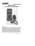
1
INTRODUCTION TO TIMS TIMS is a modular system for modelling telecommunications block diagrams. Since block diagrams themselves represent telecommunications systems, or sub-systems, and each sub-system can probably be represented by a mathematical equation, then TIMS can also be said to be a telecommunications equation modeller. Most TIMS modules perform a single function. For example, there are multipliers, adders, filters, samplers. Other modules generate signals such as sinewaves, square waves, random sequences. Complex systems are modelled by a collection of these simple modules. There are few modules that perform complex functions which otherwise could have been performed by a collection of simpler modules. conventions TIMS is almost self-explanatory, and a first-time user should have no trouble in patching up a basic system in a few minutes, without the need to refer to the extensive User Manuals. TIMS modules conform to the following conventions. • inputs to each module are located on the left hand side of the front panel • outputs from each module are located on the right hand side of the front panel • modules become powered when plugged in, and pass signals via external patch leads connecting front panel sockets • sockets involving analog signals are coloured yellow • sockets involving digital signals are coloured red • analog signals are user-adjusted to the TIMS ANALOG REFERENCE LEVEL, which is 4 volt peak-to-peak • digital signals are sent and received at TTL levels (0 volt and 5 volt) • input impedances are high (>10 kohms) and output impedances low (<150 ohms), so that interconnections do not change signal levels. • no signal can be generated by a TIMS module which could damage another module • outputs can be shortcircuited, or joined together, without causing any damage • modules can be inserted in any free slot of a system rack, where they obtain their DC power • baseband signals are typically located below 10 kHz • bandpass signals are typically located in the 100 kHz region. • most modules can perform their intended functions over the full TIMS frequency range, which extends to 1 MHz. • system noise is typically at least 40 dB below the TIMS ANALOG REFERENCE LEVEL www.emona-tims.com 1/2 Emona-TIMS introduction to TIMS L-01 rev 1.4 messages Analog systems are typically set up using single sinusoids as messages. A two-tone test signal can be modelled for more rigorous tests. A SPEECH module is instructive for other tests. A SEQUENCE GENERATOR module is used for digital messages. instrumentation TIMS is complete in itself except for one addition - an oscilloscope - which is the basic measurement tool. Since the bandwidth of TIMS signals seldom exceeds 1 MHz, a general purpose two channel oscilloscope is more than adequate. Although TIMS itself can model a wave analyser, thus showing the principles of spectrum analysis, the PICO virtual instrument plus a PC is recommended for more serious work. This instrument operates as a virtual oscilloscope as well. TIMS includes a WIDEBAND TRUE RMS METER module, with a calibrated attenuator. This is particularly useful for setting up precise signal-to-noise ratios. The in-built FREQUENCY COUNTER is used for all frequency measurements. As an event counter, with other modules, it enables precision bit error rate (BER) determinations in digital systems. experimental practice It is customary to insert modules into the TIMS frame in the order they appear in the block diagram which is to be modelled. Patching usually proceeds from input to output in a systematic manner. None of the TIMS front panel controls is calibrated. Signals are typically set up, to their appropriate frequencies and amplitudes, using the oscilloscope or WIDEBAND TRUE RMS METER. Analog signals, at module interfaces, are normally adjusted to the TIMS ANALOG REFERENCE LEVEL of 4 volt peak-to-peak. This ensures that they do not drop down to the system noise level (at last 40 dB below this), nor introduce distortion products by amplitude overload. Digital signal levels will be fixed automatically at one or other of the two standard TTL levels (either +5 or 0 volt). When it is necessary to transmit a TTL signal via an analog circuit, an ‘analog’ version is usually available. This is a ±2 volt (bi-polar) waveform derived from the TTL version. oscilloscope synchronization It is always important to consider carefully which of the many signals present will be used to trigger (synchronize) the oscilloscope. Seldom is it desirable to synchronize to the output waveform of the system itself. Typically this contains more than one frequency component, and will be of varying amplitude (as the system is adjusted, for example); this is an unsuitable signal for obtaining stable synchronization. Instead, look for a signal of fixed frequency and amplitude, and which bears an appropriate relationship to the desired signal display. For example, the message source when displaying the envelope of an amplitude modulated signal. TIMS Lab Sheet copyright tim hooper 1999, amberley holdings pty ltd ACN 001-080-093 2/2 MODELLING EQUATIONS modules basic: ADDER, AUDIO OSCILLATOR, PHASE SHIFTER optional basic: MULTIPLIER preparation This experiment assumes no prior knowledge of telecommunications. It illustrates how TIMS is used to model a mathematical equation. You will learn some experimental techniques. It will serve to introduce you to the TIMS system, and prepare you for the more serious experiments to follow. In this experiment you will model a simple trigonometrical equation. That is, you will demonstrate in hardware something with which you are already familiar analytically. This is not a typical TIMS Lab Sheet. It gives much more detail than later sheets. an equation to model You will see that what you are to do experimentally is to demonstrate that two AC signals of the same frequency, equal amplitude and opposite phase, when added, will sum to zero. This process is used frequently in communication electronics as a means of removing, or at least minimizing, unwanted components in a system. You will meet it in later experiments. The equation which you are going to model is: y(t) = V1 sin(2πf1t) + V2 sin(2πf2t + α) = v1(t) + v2(t) ........ 1 ........ 2 Here y(t) is described as the sum of two sine waves. Every young trigonometrician knows that, if: ........ 3 each is of the same frequency: f1 = f2 Hz ........ 4 each is of the same amplitude: V1 = V2 volts and they are 180o out of phase: then: α = 180 degrees y(t) = 0 ........ 5 ........ 6 A block diagram to represent eqn.(1) is suggested in Figure 1. www.emona-tims.com 1/10 Emona-TIMS modelling equations L-02 rev 1.4 SOURCE ADDER v1 (t) OUT y(t) V sin2 πf1t -1 INVERTING AMPLIFIER v (t) 2 Figure 1: block diagram model of Equation 1 Note that we ensure the two signals are of the same frequency (f1 = f2) by obtaining them from the same source. The 180 degree phase change is achieved with an inverting amplifier, of unity gain. In the block diagram of Figure 1 it is assumed, by convention, that the ADDER has unity gain between each input and the output. Thus the output is y(t) of eqn.(2). This diagram appears to satisfy the requirements for obtaining a null at the output. Now see how we could model it with TIMS modules. A suitable arrangement is illustrated in block diagram form in Figure 2. OSCILLOSCOPE and FREQUENCY COUNTER connections not shown. v (t) 2 y(t) = g.v1(t) + G.v2(t) v (t) 1 = V sin2π f1t + V2 sin2πf2t 1 Figure 2: the TIMS model of Figure 1. Before you build this model with TIMS modules let us consider the procedure you might follow in performing the experiment. the ADDER The annotation for the ADDER needs explanation. The symbol ‘G’ near input A means the signal at this input will appear at the output, amplified by a factor ‘G’. Similar remarks apply to the input labelled ‘g’. Both ‘G’ and ‘g’ are adjustable by adjacent controls on the front panel of the ADDER. But note that, like the controls on all of the other TIMS modules, these controls are not calibrated. You must adjust these gains for a desired final result by measurement. Thus the ADDER output is not identical with eqn.(2), but instead: ADDER output = g.v1(t) + G.v2(t) TIMS Lab Sheet copyright tim hooper 1999, amberley holdings pty ltd ACN 001-080-093 ........ 7 2/10 Emona-TIMS modelling equations L-02 rev 1.4 = V1 sin2πf1t + V2 sin2πf2t ........ 8 conditions for a null For a null at the output, sometimes referred to as a ‘balance’, one would be excused for thinking that: if: 1) the PHASE SHIFTER is adjusted to introduce a difference of 180o between its input and output and 2) the gains ‘g’ and ‘G’ are adjusted to equality then 3) the amplitude of the output signal y(t) will be zero. In practice the above procedure will almost certainly not result in zero output ! Here is the first important observation about the practical modelling of a theoretical concept. In a practical system there are inevitably small impairments to be accounted for. For example, the gain through the PHASE SHIFTER is approximately unity, not exactly so. It would thus be pointless to set the gains ‘g’ and ‘G’ to be precisely equal. Likewise it would be a waste of time to use an expensive phase meter to set the PHASE SHIFTER to exactly 180o, since there are always small phase shifts not accounted for elsewhere in the model. These small impairments are unknown, but they are stable. Once compensated for they produce no further problems. So we do not make precise adjustments to modules, independently of the system into which they will be incorporated, and then patch them together and expect the system to behave. All adjustments are made to the system as a whole to bring about the desired end result. more insight into the null It is instructive to express eqn. (1) in phasor form. Refer to Figure 3. TIMS Lab Sheet copyright tim hooper 1999, amberley holdings pty ltd ACN 001-080-093 3/10 Emona-TIMS modelling equations L-02 rev 1.4 Figure 3: Equation (1) in phasor form The null at the output of the simple system of Figure 2 is achieved by adjusting the uncalibrated controls of the ADDER and of the PHASE SHIFTER. Although equations (3), (4), and (5) define the necessary conditions for a null, they do not give any guidance as to how to achieve these conditions. Figure 3 (a) and (b) shows the phasors V1 and V2 at two different angles α. It is clear that, to minimise the length of the resultant phasor (V1 + V2), the angle α in (b) needs to be increased by about 45o. The resultant having reached a minimum, then V2 must be increased to approach the magnitude of V1 for an even smaller (finally zero) resultant. We knew that already. What is clarified is the condition prior to the null being achieved. Note that, as angle α is rotated through a full 360o, the resultant (V1 + V2) goes through one minimum and one maximum (refer to the TIMS User Manual to see what sort of phase range is available from the PHASE SHIFTER). What is also clear from the phasor diagram is that, when V1 and V2 differ by more than about 2:1 in magnitude, the minimum will be shallow, and the maximum broad and not pronounced 1. Thus we can conclude that, unless the magnitudes V1 and V2 are already reasonably close, it may be difficult to find the null by rotating the phase control. So, as a first step towards finding the null, it would be wise to set V2 close to V1. This will be done in the procedures detailed below. Note that, for balance, it is the ratio of the magnitudes V1 and V2 , rather than their absolute magnitudes, which is of importance. So we will consider V1 of fixed magnitude (the reference), and make all adjustments to V2. This assumes V1 is not of zero amplitude ! 1 fix V as reference; mentally rotate the phasor for V . The dashed circle shows the locus of its extremity. 1 2 TIMS Lab Sheet copyright tim hooper 1999, amberley holdings pty ltd ACN 001-080-093 4/10 Emona-TIMS modelling equations L-02 rev 1.4 experiment You are now ready to model eqn. (1). The modelling is explained step-by-step as a series of small tasks T. Take these tasks seriously, now and in later experiments, and TIMS will provide you with hours of stimulating experiences in telecommunications and beyond. The tasks are identified with a ‘T’, are numbered sequentially, and should be performed in the order given. T1 both channels of the oscilloscope should be permanently connected to the matching coaxial connectors on the SCOPE SELECTOR. See the TIMS User Manual for details of this module. T2 in this experiment you will be using three plug-in modules, namely: an AUDIO OSCILLATOR, a PHASE SHIFTER, and an ADDER. Obtain one each of these. Identify their various features as described in the TIMS User Manual. In later experiments always refer to this manual when meeting a module for the first time. Most modules can be controlled entirely from their front panels, but some have switches mounted on their circuit boards. Set these switches before plugging the modules into the TIMS SYSTEM UNIT; they will seldom require changing during the course of an experiment. T3 set the on-board range switch of the PHASE SHIFTER to ‘LO’. Its circuitry is designed to give a wide phase shift in either the audio frequency range (LO), or the 100 kHz range (HI). A few, but not many other modules, have onboard switches. These are generally set, and remain so set, at the beginning of an experiment. Always refer to the TIMS User Manual if in doubt. Modules can be inserted into any one of the twelve available slots in the TIMS SYSTEM UNIT. Choose their locations to suit yourself. Typically one would try to match their relative locations as shown in the block diagram being modelled. Once plugged in, modules are in an operating condition. When modelling large systems extra space can be obtained with an additional TIMS-301 System Unit, a TIMS-801 TIMS-Junior, or a TIMS-240 Expansion Rack. T4 plug the three modules into the TIMS SYSTEM UNIT. T5 set the front panel switch of the FREQUENCY COUNTER to a GATE This is the most common selection for measuring frequency. TIMS Lab Sheet copyright tim hooper 1999, amberley holdings pty ltd ACN 001-080-093 TIME of 1s. 5/10 Emona-TIMS modelling equations L-02 rev 1.4 When you become more familiar with TIMS you may choose to associate certain signals with particular patch lead colours. For the present, choose any colour which takes your fancy. T6 connect a patch lead from the lower yellow (analog) output of the AUDIO OSCILLATOR to the ANALOG input of the FREQUENCY COUNTER. The display will indicate the oscillator frequency f1 in kilohertz (kHz). T7 set the frequency f1 with the knob on the front panel of the AUDIO OSCILLATOR, to approximately 1 kHz (any frequency would in fact be suitable for this experiment). T8 connect a patch lead from the upper yellow (analog) output of the AUDIO OSCILLATOR to the ‘ext. trig’ [ or ‘ext. synch’ ] terminal of the oscilloscope. Make sure the oscilloscope controls are switched so as to accept this external trigger signal; use the automatic sweep mode if it is available. T9 set the sweep speed of the oscilloscope to 0.5 ms/cm. T10 patch a lead from the lower analog output of the AUDIO OSCILLATOR to the input of the PHASE SHIFTER. T11 patch a lead from the output of the PHASE SHIFTER to the input G of the ADDER 2. T12 patch a lead from the lower analog output of the AUDIO OSCILLATOR to the input g of the ADDER. T13 patch a lead from the input g of the ADDER to CH2-A of the SCOPE SELECTOR module. Set the lower toggle switch of the SCOPE SELECTOR to UP. T14 patch a lead from the input G of the ADDER to CH1-A of the SCOPE SELECTOR. Set the upper SCOPE SELECTOR toggle switch UP. T15 patch a lead from the output of the ADDER to CH1-B of the SCOPE SELECTOR. This signal, y(t), will be examined later on. Your model should be the same as that shown in Figure 4 below, which is based on Figure 2. Note that in future experiments the format of Figure 2 will be used for TIMS models, rather than the more illustrative and informal style of Figure 4, which depicts the actual flexible patching leads. You are now ready to set up some signal levels. 2 the input is labelled ‘A’, and the gain is ‘G’. This is often called ‘the input G’; likewise ‘input g’. TIMS Lab Sheet copyright tim hooper 1999, amberley holdings pty ltd ACN 001-080-093 6/10 Emona-TIMS modelling equations L-02 rev 1.4 v2(t) v (t) 1 Figure 4: the TIMS model. T16 find the sinewave on CH1-A and, using the oscilloscope controls, place it in the upper half of the screen. T17 find the sinewave on CH2-A and, using the oscilloscope controls, place it in the lower half of the screen. This will display, throughout the experiment, a constant amplitude sine wave, and act as a monitor on the signal you are working with. Two signals will be displayed. These are the signals connected to the two ADDER inputs. One goes via the PHASE SHIFTER, which has a gain whose nominal value is unity; the other is a direct connection. They will be of the same nominal amplitude. T18 vary the COARSE control of the PHASE SHIFTER, and show that the relative phases of these two signals may be adjusted. Observe the effect of the ±1800 toggle switch on the front panel of the PHASE SHIFTER. As part of the plan outlined previously it is now necessary to set the amplitudes of the two signals at the output of the ADDER to approximate equality. Comparison of eqn. (1) with Figure 2 will show that the ADDER gain control g will adjust V1, and G will adjust V2. You should set both V1 and V2, which are the magnitudes of the two signals at the ADDER output, at or near the TIMS ANALOG REFERENCE LEVEL, namely 4 volt peak-to-peak. Now let us look at these two signals at the output of the ADDER. T19 switch the SCOPE SELECTOR from CH1-A to CH1-B. Channel 1 (upper trace) is now displaying the ADDER output. T20 remove the patch cords from the g input of the ADDER. This sets the amplitude V1 at the ADDER output to zero; it will not influence the adjustment of G. T21 adjust the G gain control of the ADDER until the signal at the output of the ADDER, displayed on CH1-B of the oscilloscope, is about 4 volt peak-topeak. This is V2. TIMS Lab Sheet copyright tim hooper 1999, amberley holdings pty ltd ACN 001-080-093 7/10 Emona-TIMS modelling equations L-02 rev 1.4 T22 remove the patch cord from the G input of the ADDER. This sets the V2 output from the ADDER to zero, and so it will not influence the adjustment of g. T23 replace the patch cords previously removed from the g input of the ADDER, thus restoring V1. T24 adjust the g gain control of the ADDER until the signal at the output of the ADDER, displayed on CH1-B of the oscilloscope, is about 4 volt peak-topeak. This is V1. T25 replace the patch cords previously removed from the G input of the ADDER. Both signals (amplitudes V1 and V2) are now displayed on the upper half of the screen (CH1-B). Their individual amplitudes have been made approximately equal. Their algebraic sum may lie anywhere between zero and 8 volt peak-to-peak, depending on the value of the phase angle α. It is true that 8 volt peak-to-peak would be in excess of the TIMS ANALOG REFERENCE LEVEL, but it won`t overload the oscilloscope, and in any case will soon be reduced to a null. Your task is to adjust the model for a null at the ADDER output, as displayed on CH1-B of the oscilloscope. You may be inclined to fiddle, in a haphazard manner, with the few front panel controls available, and hope that before long a null will be achieved. You may be successful in a few moments, but this is unlikely. Such an approach is definitely not recommended if you wish to develop good experimental practices. Instead, you are advised to remember the plan discussed above. This should lead you straight to the wanted result with confidence, and the satisfaction that instant and certain success can give. There are only three conditions to be met, as defined by equations (3), (4), and (5). • the first of these is already assured, since the two signals are coming from a common oscillator. • the second is approximately met, since the gains ‘g’ and ‘G’ have been adjusted to make V1 and V2, at the ADDER output, about equal. • the third is unknown, since the front panel control of the PHASE SHIFTER is not calibrated 3. It would thus seem a good idea to start by adjusting the phase angle α. So: T26 set the FINE control of the PHASE SHIFTER to its central position. 3 TIMS philosophy is not to calibrate any controls. In this case it would not be practical, since the phase range of the PHASE SHIFTER varies with frequency. TIMS Lab Sheet copyright tim hooper 1999, amberley holdings pty ltd ACN 001-080-093 8/10 Emona-TIMS modelling equations L-02 rev 1.4 T27 whilst watching the upper trace, y(t) on CH1-B, vary the COARSE control of the PHASE SHIFTER. Unless the system is at the null or maximum already, rotation in one direction will increase the amplitude, whilst in the other will reduce it. Continue in the direction which produces a decrease, until a minimum is reached. That is, when further rotation in the same direction changes the reduction to an increase. If such a minimum can not be found before the full travel of the COARSE control is reached, then reverse the front panel 180O TOGGLE SWITCH, and repeat the procedure. Keep increasing the sensitivity of the oscilloscope CH1 amplifier, as necessary, to maintain a convenient display of y(t). Leave the PHASE SHIFTER controls in the position which gives the minimum. T28 now select the G control on the ADDER front panel to vary V2, and rotate it in the direction which produces a deeper null. Since V1 and V2 have already been made almost equal, only a small change should be necessary. T29 repeating the previous two tasks a few times should further improve the depth of the null. As the null is approached, it will be found easier to use the FINE control of the PHASE SHIFTER. These adjustments (of amplitude and phase) are NOT interactive, so you should reach your final result after only a few such repetitions. Nulling of the two signals is complete ! You have achieved your first objective You will note that it is not possible to achieve zero output from the ADDER. This never happens in a practical system. Although it is possible to reduce y(t) to zero, this cannot be observed, since it is masked by the inevitable system noise. T30 reverse the position of the PHASE SHIFTER toggle switch. Record the amplitude of y(t), which is now the absolute sum of V1 PLUS V2. Set this signal to fill the upper half of the screen. When the 1800 switch is flipped back to the null condition, with the oscilloscope gain unchanged, the null signal which remains will appear to be ‘almost zero’. signal-to-noise ratio When y(t) is reduced in amplitude, by nulling to well below the TIMS ANALOG REFERENCE LEVEL, and the sensitivity of the oscilloscope is increased, the inevitable noise becomes visible. Here noise is defined as anything we don`t want. The noise level will not be influenced by the phase cancellation process which operates on the test signal, so will remain to mask the moment when y(t) vanishes. It will be at a level considered to be negligible in the TIMS environment - say less then 10 mV peak-to-peak. How many dB below reference level is this ? TIMS Lab Sheet copyright tim hooper 1999, amberley holdings pty ltd ACN 001-080-093 9/10 Emona-TIMS modelling equations L-02 rev 1.4 Note that the nature of this noise can reveal many things. achievements Compared with some of the models you will be examining in later experiments you have just completed a very simple exercise. Yet many experimental techniques have been employed, and it is fruitful to consider some of these now, in case they have escaped your attention. • to achieve the desired proportions of two signals V1 and V2 at the output of an ADDER it is necessary to measure first one signal, then the other. Thus it is necessary to remove the patch cord from one input whilst adjusting the output from the other. Turning the unwanted signal off with the front panel gain control is not a satisfactory method, since the original gain setting would then be lost. • as the amplitude of the signal y(t) was reduced to a small value (relative to the remaining noise) it remained stationary on the screen. This was because the oscilloscope was triggering to a signal related in frequency (the same, in this case) and of constant amplitude, and was not affected by the nulling procedure. So the triggering circuits of the oscilloscope, once adjusted, remained adjusted. • choice of the oscilloscope trigger signal is important. Since the oscilloscope remained synchronized, and a copy of y(t) remained on display (CH1) throughout the procedure, you could distinguish between the signal you were nulling and the accompanying noise. • remember that the nulling procedure was focussed on the signal at the oscillator (fundamental) frequency. Depending on the nature of the remaining unwanted signals (noise) at the null condition, different conclusions can be reached. a) if the AUDIO OSCILLATOR had a significant amount of harmonic distortion, then the remaining ‘noise’ would be due to the presence of these harmonic components. It would be unlikely for them to be simultaneously nulled. The ‘noise’ would be stationary relative to the wanted signal (on CH1). The waveform of the ‘noise’ would provide a clue as to the order of the largest unwanted harmonic component (or components). b) if the remaining noise is entirely independent of the waveform of the signal on CH1, then one can make statements about the waveform purity of the AUDIO OSCILLATOR. more models Before entering the realm of telecommunications (with the help of other TIMS Lab Sheets), there are many equations familiar to you that can be modelled. For example, try demonstrating the truth of typical trigonometrical identities, such as: • • • • • cosA.cosB = ½ [ cos(A-B) + cos(A+B) ] sinA.sinB = ½ [ cos(A-B) - cos(A+B) ] sinA.cosB = ½ [ sin(A-B) + sin(A+B) ] cos2A = ½ + ½ cos2A sin2A = ½ - ½ cos2A In the telecommunications context cosA and sinA are interpreted as electrical signals, with amplitudes, frequencies, and phases. You will need to interpret the difference between cosA and sinA in this context. When multiplying two signals there will be the need to include and account for the scale factor ‘k’ of the multiplier (see the TIMS User Manual for a definition of MULTIPLIER scale factor); and so on. TIMS Lab Sheet copyright tim hooper 1999, amberley holdings pty ltd ACN 001-080-093 10/10 DSBSC - GENERATION modules basic: MULTIPLIER optional basic: AUDIO OSCILLATOR, ADDER preparation A double sideband suppressed carrier (DSBSC) signal is defined as: ........ 1 DSBSC = a(t).cosωt where typically the frequency components in a(t), the message, all lie well below the frequency of ω. The DSBSC occupies a band of frequencies either side of ω, by amounts equal to the bandwidth of a(t). This is easy to show, for the simple case where a(t) = cosµt, by making the substitution and expanding eqn(1) to eqn(2) ........ 2 DSBSC = ½.cos(ω−µ)t + ½.cos(ω+µ)t Equation (2) is very simply generated by the arrangement of Figure 1. DSBSC message source ( µ ) carrier source (ω ) DSBSC + pilot carrier typically ω >> µ Figure 1: a DSBSC generator Here the message source a(t) is shown as a single sinusoid. typically be much less than that of the carrier source (ω). Its frequency (µ) would A snap-shot of the waveform of a DSBSC is shown in Figure 2, together with the message from which it was derived.. +1 message 0 -1 E DSBSC time -E Figure 2: a DSBSC - seen in the time domain www.emona-tims.com 1/2 Emona-TIMS DSBSC - generation L-03 rev 1.3 experiment Model the block diagram of Figure 1 as shown in Figure 3. If an AUDIO OSCILLATOR is not available, the 2 kHz MESSAGE from MASTER SIGNALS can be substituted. But this would be a special case, since this message is synchronous with the carrier frequency. Note also the optional ADDER in Figure 3; this makes provision for a ‘pilot’ carrier - see pilot carrier below. message source (µ ) optional DSB carrier source from MASTER SIGNALS ( ω) Figure 3: the TIMS model of Figure 1 There should be no trouble in viewing the output of the above generator, and displaying it as shown in Figure 4. Ideally the oscilloscope should be synchronised to the message waveform. Figure 4: typical display of a DSBSC and the message. This is not the same as the snap-shot illustrated in Figure 2. An oscilloscope with the ability to capture and display the signal over a few message periods could reproduce the display of Figure 2. You can obtain the snap-shot-like display with a ‘standard’ oscilloscope, provided the frequency ratio of the message is a sub multiple of that of the carrier. This can be achieved with difficulty by manual adjustment of the message frequency. A better solution is to use the 2 kHz MESSAGE from MASTER SIGNALS. The frequency of this signal is exactly 1/48 of the carrier. If an AUDIO OSCILLATOR is not available (the 2 kHz MESSAGE from MASTER SIGNALS being used as the message) then the display of Figure 4 will not be possible. pilot carrier For synchronous demodulators a local, synchronous carrier is required. See the Lab Sheet entitled Product demodulation, for example. As an aid to the carrier acquisition circuitry at the receiver a small amount of ‘pilot’ carrier is often inserted into the DSBSC at the transmitter (see Figure 1). Provision for this is made in the model of Figure 3. TIMS Lab Sheet copyright tim hooper 1999, amberley holdings pty ltd ACN 001-080-093 2/2 PRODUCT DEMODULATION modules basic: for the demodulator MULTIPLIER, PHASE SHIFTER, VCO basic: for the signal sources ADDER, MULTIPLIER, PHASE SHIFTER optional basic: AUDIO OSCILLATOR preparation The product demodulator is defined by the block diagram of Figure 1. message out modulated signal in carrier source phase shifter Figure 1: a product demodulator The carrier source must be locked in frequency to the carrier (suppressed or otherwise) of the incoming signal. This will be arranged by ‘stealing’ a carrier signal from the source of the modulated signal. In practice this carrier signal must be derived from the received signal itself, using carrier acquisition circuitry. This is examined in other Lab Sheets - for example, Carrier acquisition - PLL. Being an investigation of a demodulator, this experiment requires that you have available for demodulation a choice of signals. These can come from the TIMS TRUNKS system (if available), an adjacent TIMS bay, or your own TIMS system. The latter case will be assumed . You will need to know how to generate separately AM and DSBSC signals based on a 100 kHz (ω) carrier and derived from a sinusoidal message (µ). See the Lab Sheets AM - amplitude modulation and DSBSC - generation. Since an SSB signal so derived is itself just a single sinewave, at either (ω ± µ), it can be simulated by the sinusoidal output from a VCO. Set it to say 102 kHz. Remember that in the experiment to follow the message will be a single sine wave. This is very useful for many measurements, but speech would also be very revealing. If you do not have a speech source it is still possible to speculate on what the consequences would be. experiment The block diagram of Figure 1 is shown modelled by TIMS in Figure 2. Not shown is the source of input modulated signal, which you will have generated yourself. It will use the 100 kHz source from MASTER SIGNALS. This will also be the source of ‘stolen carrier’. www.emona-tims.com 1/2 Emona-TIMS Product demodulation L-04 rev 1.3 The sinusoidal message at the transmitter should be in the range 300 to 3000 kHz, say, to cover the range of a speech signal. The 3 kHz LPF in the HEADPHONE AMPLIFIER is compatible with this frequency range. IN OUT stolen carrier Figure 2: the TIMS model of Figure 1 synchronous carrier Initially use a stolen carrier; that is, one synchronous with the received signal. DSBSC input Notice that the phase of the stolen carrier plays a significant role. It can reduce the message output amplitude to zero. Not very useful here, but most desirable in other applications. Think about it. SSB input Notice that the phase of the stolen carrier has no effect upon the amplitude of the message output. But it must do something ? Investigate. Since this system appears to successfully demodulate the SSB signal, could it be called an SSB demodulator ? Strictly no ! It cannot differentiate between an upper and a lower sideband. Thus, if the input is an independent sideband (ISB) signal, it would fail. Consider this. AM input Compare with the case where the input was a DSBSC. What difference is there now ? An envelope detector will give a distorted output when the depth of modulation (m) of the AM signal exceeds unity. What will happen to the output with a product demodulator ? Investigate. non-synchronous carrier Repeat all of the above, but with a non-synchronous carrier from a VCO. Observe the consequences, especially with a small frequency error (say a few Hertz). DSBSC and SSB differ quite remarkably – especially noticeable with speech. Refer to the TIMS User Manual for fine tuning details of the VCO. In summary: • coarse tuning is accomplished with the front panel fo control (typically with no input connected to Vin). • for fine tuning set the GAIN control of the VCO to some small value. Tune with a DC voltage, from the VARIABLE DC module, connected to the Vin input. The smaller the GAIN setting the finer is the tuning. TIMS Lab Sheet copyright tim hooper 1999, amberley holdings pty ltd ACN 001-080-093 2/2 AM - AMPLITUDE MODULATION - I modules basic: ADDER, MULTIPLIER optional basic: AUDIO OSCILLATOR preparation An amplitude modulated signal is defined as: AM = E (1 + m.cosµt) cosωt ........ 1 = A (1 + m.cosµt) ........ 2 B cosωt ........ 3 = [low frequency term a(t)] x [high frequency term c(t)] Here: ‘E’ is the AM signal amplitude from eqn. (1). For modelling convenience eqn. (1) has been written into two parts in eqn. (2), where (A.B) = E. ‘m’ is a constant, which, as will be seen, defines the ‘depth of modulation’. Typically m < 1. Depth of modulation, expressed as a percentage, is 100.m. There is no inherent restriction upon the size of ‘m’ in eqn. (1). ‘µ µ’ and ‘ω ω’ are angular frequencies in rad/s, where µ/(2.π) is a low, or message frequency, say in the range 300 Hz to 3000 Hz; and ω/(2.π) is a radio, or relatively high, ‘carrier’ frequency. In TIMS the carrier frequency is generally 100 kHz. block diagram Equation (2) can be represented by the block diagram of Figure 1. G a(t) AM m(t) g message sinewave (µ ) c(t) DC voltage carrier sinewave ( ω) Figure 1: generation of AM www.emona-tims.com 1/2 Emona-TIMS AM - amplitude modulation - I L-05 rev 1.3 model CH1-B ext trig CH1-A the message (say 1kHz) CH2-A AM out 100kHz MASTER SIGNAL VARIABLE DC Figure 2: model of Figure 1 If no AUDIO OSCILLATOR is available the 2 kHz message from MASTER SIGNALS can be used instead (although this is a special case, being synchronous with the carrier). experiment To make a 100% amplitude modulated signal adjust the ADDER output voltages independently to +1 volt DC and 1 volt peak of the sinusoidal message. Figure 3 illustrates what the oscilloscope will show. tim e Figure 3 - AM, with m = 1, as seen on the oscilloscope The depth of modulation ‘m’ can be measured either by taking the ratio of the amplitude of the AC and DC terms at the ADDER output, or applying the formula: m= P−Q P+Q ........ 4 where P and Q are the peak-to-peak and trough-to-trough amplitudes respectively of the AM waveform of Figure 3. Note that Q = 0 for the case m = 1. To vary the depth of modulation use the G gain control of the ADDER. Notice that the ‘envelope’, or outline shape, of the AM signal of Figure 3 is the same as that of the message provided that m ≤ 1 . The envelope of the AM signal is defined as |a(t)|. When m ≤ 1 the envelope shape and the message shape are the same. When m > 1 the envelope is still defined as |a(t)|, but it is no longer the same shape as the message (see opposite, for the case m = 1.5). Note that eqn.(4) is still applicable - the trough is interpreted as being negative. TIMS Lab Sheet copyright tim hooper 1999, amberley holdings pty ltd ACN 001-080-093 2/2 AM - AMPLITUDE MODULATION II modules basic: ADDER, MULTIPLIER, PHASE SHIFTER basic optional: AUDIO OSCILLATOR preparation In the Lab Sheet entitled AM - amplitude modulation an amplitude modulated signal was defined as in eqn(1). ........ 1 AM = E.(1 + m.cosµt).cosωt There are other methods of writing this equation; for example, by expansion, it becomes: ........ 2 AM = E.m.cosµt.cosωt + E.cosωt ........ 3 = DSBSC + carrier The depth of modulation ‘m’ is determined by the ratio of the DSBSC and carrier amplitudes, since, from eqns.(2) and (3): ........ 4 ratio (DSBSC/carrier) = (E.m) / E = m The important practical detail here is the need to adjust the relative phase between the DSBSC and the carrier. This is not shown explicitly in eqn. (2), but is made clear by rewriting this as: ........ 5 AM = E.m.cosµt.cosωt + E.cos(ωt + α) Here α is the above mentioned phase, which, for AM, must be set to: α = 0o ........ 6 Any attempt to model eqn. (2) by adding a DSBSC to a carrier cannot assume the correct relative phases will be achieved automatically. It is eqn. (5) which will be achieved in the first instance, with the need for adjustment of the phase angle α to zero. A block diagram of an arrangement for modelling eqn. (3) is shown in Figure 1. DSBSC message (µ) g G carrier (100kHz) (ω) AM out carrier typically ω >> µ adjust phase Figure 1: block diagram of AM generator www.emona-tims.com 1/2 Emona-TIMS AM - amplitude modulation II L-06 rev 1.3 experiment The block diagram of Figure 1 can be modelled by the arrangement of Figure 2. The optional AUDIO OSCILLATOR is shown providing the message, rather than the 2 kHz MESSAGE available from MASTER SIGNALS. CH1-A ext. trig CH2-A sinω t cosω t Figure 2: the AM generator model An adequate method of phase adjustment, which requires only an oscilloscope, is to first set the peak amplitude of the DSBSC and the carrier terms to equality. This means 100% amplitude modulation, assuming the correct phase. Only when the phase is zero can the envelope troughs be made to ‘kiss’ as the phase is rotated. Try it. Examination of the signals represented in phasor form explains the phenomenon. α Am Am 2 2 A Am 2 A phase = 0 phase = Phasor Form α ω− µ ω ω + µ frequency Amplitude Spectrum Figure 3: DSBSC + carrier, with m = 1 Refer to Figure 3. It is clear that, when the phase angle α is other than zero, no matter what the sideband amplitude, they could never add with the carrier to produce a resultant of zero amplitude, which is required for the ‘kiss’. When the sidebands are in phase with the carrier, this can clearly only happen when m = 1 (as it is in the diagram). Figure 3 also shows the amplitude spectrum. This is not affected as the phase changes. There are other methods of phase adjustment. For example: recover the envelope in an envelope detector (see later experiments) and adjust the phase until the distortion of the recovered envelope is a minimum. This is a practical method which achieves directly what is desired - without ever having to measure relative phase. In this way there may be some compensation for the inevitable distortion introduced both by the transmitter, at high depths of modulation, and the receiver. Would the adjustment be simplified if you had a phase meter ? Probably not ! Think about it. TIMS Lab Sheet copyright tim hooper 1999, amberley holdings pty ltd ACN 001-080-093 2/2 ENVELOPE DETECTION modules basic: ADDER, MULTIPLIER, UTILITIES, TUNEABLE LPF optional basic: AUDIO OSCILLATOR, 60 kHz LPF preparation An envelope detector is typically used for recovering the message from the envelope of an amplitude modulated (AM) signal. In its most simple realization it consists of a diode, a capacitor, and a resistor. This is an approximation to the ideal envelope detector, which consists of a rectifier and a lowpass filter (LPF). In this experiment the ideal realization will first be examined. This is illustrated in the block diagram of Figure 1. The rectifier here operates as a device which generates the absolute value of its input. in rectifier LPF envelope out Figure 1: the ideal envelope recovery arrangement The block diagram of Figure 1 is shown modelled in Figure 2. AM in envelope out Figure 2: modelling the ideal envelope detector experiment As an input to the envelope detector you will need to make yourself an AM signal. This can be done with the message source from the MASTER SIGNALS module (or the optional AUDIO OSCILLATOR), an ADDER, and a MULTIPLIER. See the Lab Sheet entitled AM - amplitude modulation. With say a 2 kHz message to the AM generator, a depth of modulation of about 50%, and the LPF of the envelope detector set to as wide a bandwidth as possible (about 12 kHz), show that the envelope detector output is indeed a faithful copy of the message. www.emona-tims.com 1/2 Emona-TIMS envelope detection L-07 rev 1.3 Now investigate the following: 1. increase the depth of modulation to 100% 2. increase the depth of modulation beyond 100%. Even though the envelope of the input signal is no longer a faithful copy of the message, the output of the envelope detector should still be a faithful copy of the envelope. However, this will only be so if the bandwidth of the LPF is wide enough. How wide ? 3. remove the DC component from the ADDER of the AM generator. This makes a double sideband suppressed carrier (DSBSC) signal. Even if you have not met this signal before you can still observe if the envelope detector can recover its envelope. Once again, the bandwidth of the LPF must be ‘appropriate’. A 60 kHz LPF would be a better choice for this case. the ‘diode detector’ In practice the envelope detector is often realized with only a single diode and RC filter. This can also be modelled with TIMS, as shown in Figure 3. Repeat the observations made previously with the ideal realization of the envelope detector. Note and explain the difference in performance. AM in OUT approximate envelope Figure 3: approximation to an ideal envelope detector Remember that the diode detector requires a number of approximations to be met, including that the carrier frequency should be very much larger than the message frequency. This inequality does not hold true in the present case. note on envelopes AM = E (1 + m.cosµt) cosωt = a(t) cosωt ........ 1 ........ 2 Eqn.(1) above defines an AM signal, provided m ≤ 1 . It is generally agreed that a further condition is that ω >> µ. In more general terms eqn.(1) can be written as eqn.(2). By definition a signal of the form of eqn.(2) has an envelope defined by the absolute value of a(t). Generally the carrier frequency ω is much greater than the frequency of any of the terms in a(t). Even when this is not the case |a(t)| still defines the envelope, although it may then be difficult to visualize. Check this out ! For example, use an AUDIO OSCILLATOR or VCO for the carrier source, and the 2 kHz MESSAGE from MASTER SIGNALS for the message. Synchronize the oscilloscope to the message, and display the message on one channel, the AM signal on the other. .Start with the VCO (carrier) at, say, 100kHz. Demonstrate that the envelope of the AM fits exactly the shape of the message. Now switch the VCO to the top of its low frequency range. Note that the envelope still fits within the outline defined by the message. Slowly lower the carrier frequency towards that of the message. Describe what happens. Is the ‘envelope’ still defined as before ? TIMS Lab Sheet copyright tim hooper 1999, amberley holdings pty ltd ACN 001-080-093 2/2 SSB GENERATION modules basic: ADDER, AUDIO OSCILLATOR, 2 x MULTIPLIER, PHASE SHIFTER QPS preparation SSB message source DSBSC carrier source Figure 1: SSB generation by bandpass filtering A double sideband suppressed carrier (DSBSC) signal can be converted to a single sideband by the removal of one sideband. The most obvious (?) method of sideband removal is with a bandpass filter as shown in Figure 1 above. This is simple in conception, yet requires a far-from-simple filter for its execution. See historical note below. A second method of sideband removal is to make two DSBSC signals, identical in all respects except for their relative phasing. If this is suitably arranged the two DSBSC can be added, whereupon the two upper sidebands (say) cancel, whilst the two lower add. An arrangement for achieving this is illustrated in Figure 2. I DSB I π/ 2 QPS cosµ t Q (message) I cos ω t Q Σ SSB DSB Q Figure 2: SSB generation using the phasing method The block labelled ‘QPS’ is a quadrature phase splitter. This produces two output signals, I and Q, from a single input. These two are in phase quadrature. In the position shown in the diagram it will be clear that this phase relationship must be maintained over the bandwidth of the message. So it is a wideband phase splitter. www.emona-tims.com 1/2 Emona-TIMS SSB generation L-08 rev 1.3 There is another quadrature phase shifter in the diagram, but this works at one frequency only - that of the carrier. Wideband phase shifters (Hilbert transformers) are difficult to design. The phase splitter is a compromise. Although it maintains a (relatively) constant phase difference of 900 between its two outputs, there is a variable (with frequency) phase shift between either output and the common input. This is acceptable for speech signals (speech quality and recognition are not affected by phase errors) but not good for phase-sensitive data transmission. experiment The arrangement of Figure 3 is a model of the block diagram of Figure 2. CH1-A ext. trig CH2-A 100kHz from MASTER SIGNALS Figure 3: the SSB phasing generator model Notice that the suggested triggering signal for the oscilloscope is the message. To align this generator it is a simple matter to observe first the ‘upper’ DSBSC (upper in the sense of the ADDER inputs), and then the lower. Adjust each one separately (by removing the appropriate patch lead from the ADDER input) to have the same output amplitudes (say 4 volt peak-to-peak) Then replace both ADDER inputs, and watch the ADDER output as the PHASE SHIFTER is adjusted. The desired output is a single sinewave, so adjust for a flat envelope. A fine trim of one or other of the ADDER gain controls will probably be necessary. The gain and phase adjustments are non-interactive. The magnitude of the remaining envelope will indicate, and can be used analytically, to determine the ratio of wanted to unwanted sideband in the output. This will not be infinite ! The QPS, which cannot be adjusted, will set the ultimate performance of the system. Which sideband has been produced ? This can be predicted analytically by measuring the relative phases of all signals. Alternatively, measure it ! Presumably it will be either (ω − µ) or (ω + µ) rad/s. Demonstrate your knowledge of the system by re-adjusting it to produce the opposite sideband. Vary the message frequency and see if the system performs adequately over the full frequency range available. Which module is most likely to limit the system bandwidth ? historical note: today it is a digital world. Frequency division multiplex (FDM) has been almost entirely replaced by time division multiplex (TDM). As the FDM systems were de-commissioned the market was flooded with SSB filters. Some were in the range 64 to 108 kHz. They were ideal for TIMS, and very cheap. Unfortunately the supply has dried up (?), and currently available SSB filters for TIMS are prohibitively expensive. Thus for SSB purposes TIMS uses the less expensive QPS. TIMS Lab Sheet copyright tim hooper 1999, amberley holdings pty ltd ACN 001-080-093 2/2 SSB DEMODULATION modules: basic: basic: for demodulation ADDER, 2 x MULTIPLIER, QPS for transmission VCO preparation An SSB signal can be demodulated with a product demodulator. See the Lab Sheet entitled Product demodulation. But a product demodulator is not an SSB demodulator in the strict sense. A true SSB demodulator can distinguish between a lower sideband and an upper sideband. This experiment investigates the phasing type demodulator, block diagrams of which are shown in Figure 1. It would be helpful, though not essential, that the Lab Sheet entitled SSB generation has been completed. QPS I I in π/2 ω0 Σ message out bandwidth B Hz. π/2 ω0 IN π I Σ message OUT 2 QPS Q Q Q Figure 1: ideal (left) and practical (right) phasing-type SSB demodulator The 90 degree phase shifter in the lower - Q - arm of the structure (left block) needs to introduce a 90 degree phase shift over all frequencies of interest. In this case these are those of the message. Such a ‘filter’ is difficult to realize. A practical solution is the quadrature phase splitter - QPS - shown in the right block. This maintains a 90 degree shift between its outputs, although the phase difference between one input and either output varies with frequency. This variation is acceptable when the message is speech. Note that ideally there should be identical lowpass filters in each multiplier output. In practice a single lowpass filter is inserted in the summing output. The practical advantage of this is a saving of components (modules). One disadvantage of this is that the QPS will be presented with larger-than-necessary signals at its inputs - the unwanted sum frequency components as well as the wanted difference frequency components. Unwanted components increase the risk of overload. www.emona-tims.com 1/2 Emona-TIMS SSB demodulation L-09 rev 1.3 experiment A model of the block diagram of Figure 1 is shown in Figure 2. CH1-A IN 100kHz signals QUADRATURE PHASE LOCAL CARRIER Figure 2: model of a phasing-type SSB demodulator An SSB received signal is required. If such a signal were derived from a single tone message, and based on a 100 kHz (suppressed) carrier, it can be simulated by a single sinewave either just above or just below 100 kHz. This can be obtained from a VCO. After patching up the model it is necessary to align it. With an input signal (VCO) at, say, 102 kHz (simulating an upper sideband): 1. examine the waveforms throughout the model. Most will be un-familiar. 2. use the oscilloscope to set the phase shift through the PHASE SHIFTER to about 900. 3. with only one input at a time into the ADDER, set its output to say 2 volt peak-to-peak. 4. connect both inputs to the ADDER. Minimize the output from the LPF by alternately adjusting the PHASE SHIFTER and one ADDER gain control (why not maximize the ADDER output in the above procedure ?). The above procedure used an upper sideband for alignment. lower sideband of a 100 kHz carrier. It is now set to receive the Verify this by tuning the VCO to the region of the lower sideband. Alternatively, institute what ever change you think is necessary to swap from one sideband reception to the other. Conversion of the summer from an ADDER to a SUBTRACTOR would do it (insert a BUFFER AMPLIFIER, which acts as an inverter, into one path to the ADDER) ; what other methods are there ? Notice that by removing one input from the ADDER you have a DSBSC receiver. Observe that it will still demodulate the simulated SSB. So why bother with the complication of using the QPS for SSB reception ? TIMS Lab Sheet copyright tim hooper 1999, amberley holdings pty ltd ACN 001-080-093 2/2 ISB - INDEPENDENT SIDEBAND modules basic: see text. A possible minimum would be: ISB transmitter: ADDER, 2*VCO ISB receiver: ADDER, 2*MULTIPLIER, QPS carrier acquisition: MULTIPLIER, UTILITIES, VCO preparation An independent sideband - ISB - signal consists of two independent single sideband (SSB) signals based on the same - suppressed - carrier, but on opposite sides (USSB and LSSB). Sometimes each of these sidebands can themselves be two or more independent sidebands located adjacent to each other (as in an FDM system). What ever sideband arrangement is chosen, the point is that the receiver needs to recover only a single carrier. ISB was popular in the early days of SSB, since it simplified the receiver design in regard to carrier acquisition. Instead of requiring the acquisition of one carrier for each channel, only one carrier need be provided for all channels (typically only two). With the advent of frequency synthesisers, and the ease of obtaining enormously improved carrier stability, this advantages offered by ISB is no longer of consequence. A two channel ISB signal can be made by adding two SSB - one an upper sideband (USSB), and the other a lower sideband (LSSB), of a common carrier. The block diagram of Figure 1 illustrates such an arrangement, with the provision for the addition of a small amount of ‘pilot’ carrier, for the carrier acquisition circuitry of the receiver. USSB generator message #1 ISB message #2 LSSB generator Figure 1: ISB generator, with pilot carrier A suitable model for generating the USSB and the LSSB is described in the Lab Sheet entitled SSB generation. Weaver`s method - Weaver`s SSB generator - is unnecessarily complex. In similar vein, an ISB receiver consists of two SSB receivers, one tuned to the USSB, the other to the LSSB. A single carrier acquisition circuit acquires the same carrier for each. This is illustrated in block diagram form in Figure 2. www.emona-tims.com 1/2 Emona-TIMS ISB - independent sideband L-10 rev 1.3 USSB receiver ISB IN message #1 out carrier acquisition message #2 out LSSB receiver Figure 2: an ISB receiver, with carrier acquisition circuitry A suitable model for receiving either the USSB or the LSSB is described in the Lab Sheets entitled SSB demodulation. Models of the block diagrams of Figure 1 and Figure 2 are given in the associated Lab Sheets, and will not be reproduced here. In the receiver, use the LPF in the HEADPHONE AMPLIFIER. What of the carrier acquisition circuitry ? entitled Carrier acquisition - PLL. One method is described in the Lab Sheet experiment A suitable model can take several forms, depending on which generator is chosen, and which receiver. A phasing transmitter and a phasing receiver would be the most simple options if a complete system is to be modelled. However, several simplifications are possible. Each sideband generator can be simulated with a single VCO. For example, a VCO tuned, say, to 102 kHz, would represent an USSB transmitter, with a carrier of 100 kHz, and a 2 kHz message. A second VCO could, likewise, simulate the LSSB signal. The two VCO signals would then be added. The ISB receiver can be demonstrated without actually building a complete system. For example, only one receiver need be modelled. That can be modified (eg, a carrier phase change), to demonstrate the ability to receive either the USSB or the LSSB of the ISB. The module requirements at the head of this sheet assumes such simplifications. The receiver could be aligned while using a stolen carrier. Then, when satisfied, patch up the carrier acquisition circuitry. This is the most critical element of the receiver. The most difficult task for it would be to acquire the carrier when only one sideband is present. Experiment with the level of pilot carrier to be inserted at the transmitter. In commercial practice this is typically 20 dB below the peak sideband level. As a final test of the receiver it must be demonstrated that it can be adjusted to receive each channel independently of the other. If only one half of the receiver has been modelled: 1. remove, say, the lower sideband, from the transmitted signal 2. demonstrate reception of the upper sideband 3. switch to receive the lower sideband, leaving the upper sideband at the input, and show that there is no (or negligible) output TIMS Lab Sheet copyright tim hooper 1999, amberley holdings pty ltd ACN 001-080-093 2/2 ARMSTRONG`S PHASE MODULATOR modules basic: ADDER, MULTIPLIER, PHASE SHIFTER optional basic: AUDIO OSCILLATOR, UTILITIES preparation Armstrong's modulator is basically a phase modulator. The more familiar amplitude modulated signal is defined as: AM = E.(1 + m.sinµt).sinωt ...... 1 This expression can be expanded trigonometrically into the sum of two terms: AM = E.sinωt + E.m.sinµt.sinωt ...... 2 In eqn.(2) the two terms involved with 'ω' - the higher frequency term - are in phase. Now this relation can easily be changed so that the two are at 90 degrees, or in quadrature. This is done by changing one of the sinωt terms to cosωt. The signal then becomes Armstrong`s signal. Thus: Armstrong`s signal = E.cosωt + E.m.sinµt.sinωt ...... 3 This is represented in block diagram form in Figure 1. DSBSC message (sine wave) g Armstrong`s signal (µ ) G 100 kHz (sine wave) (ω) carrier typically ω >> µ adjust phase Figure 1: Armstrong`s phase modulator Apart from Armstrong`s original paper, the signal is well described by D.L. Jaffe ‘Armstrong`s Frequency Modulator’, Proc.IRE, Vol.26, No.4, April 1938, pp475-481. It can be shown that this is a phase modulated signal with a peak phase deviation ∆φ, where: ∆φ = arctan(DSBSC/CARRIER)radians ...... 4 To keep the phase deviation ∆φ approximately proportional to the amplitude of the message (from which the DSBSC is derived) it is necessary that the ratio DSBSC/CARRIER is kept small so that ∆φ ≈ DSBSC/CARRIER www.emona-tims.com 1/2 Emona-TIMS Armstrong`s phase modulator L-11 rev 1.3 experiment Figure 2 shows a model of the block diagram of Figure 1. You may use the 2 kHz message from MASTER SIGNALS if an AUDIO OSCILLATOR is not available. CH1-A ext. trig CH2-A 100kHz from MASTER SIGNALS Figure 2: the model of Armstrong`s modulator There are only two adjustments to be made. 1. set the amplitude ratio of DSBSC to carrier, at the ADDER output, as required 2. set the phase between the DSBSC and carrier to 900 The first of these is easy. How to achieve the second ? Look at the waveforms of Figure 3. They will give a clue. There are other methods. Figure 3: Armstrong’s signal, with ∆φ = 1 (eqn 3), and DSBSC to carrier phases of 450 (lower), 700 (centre) and 900 (upper). amplitude limiting The spectrum at the output of the ADDER (Figure 2) has just three components - two from the DSBSC, and one from the carrier term. Use the CLIPPER in the UTILITIES module to introduce amplitude limiting. Set it in the hard limit mode (see the TIMS User Manual). You could build a WAVE ANALYSER (see the Lab Sheet entitled The WAVE ANALYSER) else use the PICO SPECTRUM ANALYSER to confirm the introduction of new spectral components. Use your theory to predict the amplitude of these components. TIMS Lab Sheet copyright tim hooper 1999, amberley holdings pty ltd ACN 001-080-093 2/2 FM - GENERATION BY VCO modules: basic: VCO optional basic: AUDIO OSCILLATOR preparation A very simple and direct method of generating an FM signal is by the use of a voltage controlled oscillator -VCO. The frequency of such an oscillator can be varied by an amount proportional to the magnitude of an input (control) voltage. Such oscillators, in the form of an integrated circuit, have very linear characteristics over a frequency range which is a significant percentage of the centre frequency. Despite the above desirable characteristic, the VCO fails in one respect as a generator of FM - the stability of its centre frequency is not acceptable for most communication purposes. It is hardly necessary to show the block diagram of such an FM generator ! See Figure 1(a). VCO FM OUT message IN (a) (b) Figure 1: FM by VCO (a), and resulting output (b). Figure 1(b) shows a snap shot time domain display of an FM signal, together with the message from which it was derived. The frequency change is large compared with the unmodulated output frequency, and the carrier frequency is only four times that of the message. So this waveform is not a typical one. But it can be reproduced with TIMS. Note particularly that there are no amplitude variations - the envelope of an FM waveform is a constant. experiment A model of the VCO method of generation is shown in Figure 2. Note that the on-board switch SW2 must be set to ‘VCO’. FM OUT Figure 2: FM generation by VCO The message is shown coming from an AUDIO OSCILLATOR, but the 2 kHz sine wave from MASTER SIGNALS can be used instead. www.emona-tims.com 1/2 Emona-TIMS FM - generation by VCO L-12 rev 1.3 deviation calibration Before generating an FM waveform it is interesting to determine the deviation sensitivity and linearity - of the VCO. Use the front panel ‘f0’ control to set the output frequency close to 100 kHz. Instead of using a sinewave as the message, connect instead the VARIABLE DC voltage to the input Vin of the VCO. The deviation sensitivity can be set with the front panel GAIN control. Set this to about 20% of its fully clockwise rotation. Vary the VARIABLE DC at the Vin socket of the VCO and plot frequency variation versus both negative and positive values of Vin. If this is reasonably linear over the full DC range then increase the GAIN control (sensitivity) setting of the VCO and repeat. The aim is to determine the extent of the linear range, restricting the DC voltage to the TIMS ANALOG REFERENCE LEVEL of 4 volt peak-to-peak. 10 kHz deviation Using the previous results, set up the VCO to a ±10 kHz frequency deviation from a signal at the TIMS ANALOG REFERENCE LEVEL of 4 volts peak-to-peak. Alternatively: 1. set the DC voltage to ±2 volts 2. set the GAIN control fully anti-clockwise, and the output frequency to 100 kHz 3. advance the GAIN control until the frequency changes by 10 kHz. sinusoidal messages Replace the DC voltage source with the output from an AUDIO OSCILLATOR. The frequency deviation will now be about ±10 kHz, since the oscillator output is about 2 volt peak. To display a waveform of the type illustrated in Figure 1(b) is not easy with a basic oscilloscope, but glimpses may be obtained by slowly varying the message frequency over the range say 1.5 kHz to 2.5 kHz. spectrum analysis If you have a PICO SPECTRUM ANALYSER, and are familiar with the theory of the FM spectrum, many interesting observations can be made. In particular, confirmation of some of the theory is possible by adjusting the deviation to the special values predicted by their ‘Bessel zeros’. The TIMS Lab Sheet entitled FM and Bessel zeros demonstrates these phenomena by modelling a simple WAVE ANALYSER. stable carrier If the stability of the centre frequency of a VCO is un-acceptable for communications purposes then an Armstrong modulator is an alternative. This is examined in the Lab Sheet entitled Armstrong`s frequency modulator. TIMS Lab Sheet copyright tim hooper 1999, amberley holdings pty ltd ACN 001-080-093 2/2 FM - DEMODULATION BY PLL modules: basic: for demodulation MULTIPLIER, UTILITIES, VCO basic: for generation VCO preparation This experiment examines the phase locked loop as an FM demodulator. Figure 1 shows a block diagram of the arrangement to be examined. LPF FM in message out VCO Figure 1: the PLL The principle of operation is simple - or so it would appear. Consider the arrangement of Figure 1 in open loop form. That is, the connection between the filter output and VCO control voltage input is broken. Suppose there is an unmodulated carrier at the input. The arrangement is reminiscent of a product, or multiplier-type, demodulator. If the VCO was tuned precisely to the frequency of the incoming carrier, ω0 say, then the output would be a DC voltage, of magnitude depending on the phase difference between itself and the incoming carrier. For two angles within the 3600 range the output would be precisely zero volts DC. Now suppose the VCO started to drift slowly off in frequency. Depending upon which way it drifted, the output voltage would be a slowly varying AC, which if slow enough looks like a varying amplitude DC. The sign of this DC voltage would depend upon the direction of drift. Suppose now that the loop of Figure 1 is closed. If the sign of the slowly varying DC voltage, now a VCO control voltage, is so arranged that it is in the direction to urge the VCO back to the incoming carrier frequency ω0, then the VCO would be encouraged to ‘lock on’ to the incoming carrier. This is a method of carrier acquisition. Next suppose that the incoming carrier is frequency modulated. For a low frequency message, and small deviation, you can imagine that the VCO will endeavour to follow the incoming carrier frequency. What about wideband FM ? With ‘appropriate design’ of the lowpass filter and VCO circuitry the VCO will follow the incoming carrier for this too. www.emona-tims.com 1/2 Emona-TIMS FM - demodulation by PLL L-13 rev 1.3 The control voltage to the VCO will endeavour to keep the VCO frequency locked to the incoming carrier, and thus will be an exact copy of the original message. The above concepts can be examined by modelling a PLL. experiment To test the PLL use the output from the generator described in the Lab Sheet entitled FM generation by VCO. Set up the generator as described there, with a carrier in the vicinity of 100 kHz. Set it to a known frequency deviation. Then: 1. model the demodulator as illustrated in Figure 2. message OUT FM IN Figure 2: the PLL model 2. set up the VCO module in 100 kHz VCO mode. In the first instance set the front panel GAIN control to its mid-range position. 3. connect the output of the generator to the input of the demodulator 4. the PLL may or may not at once lock on to the incoming FM signal. This will depend upon several factors, including: • • • the frequency to which the PLL is tuned the capture range of the PLL the PLL loop gain - the setting of the front panel GAIN control of the VCO You will also need to know what method you will use to verify that lock has taken place. 5. make any necessary adjustments to the PLL to obtain lock, and record how this was done. Measure the amplitude and frequency of the recovered message (if periodic), or otherwise describe it (speech or music ?). 6. compare the waveform and frequency of the message at the transmitter, and the message from the demodulator. 7. check the relationship between the message amplitude at the transmitter, and the message amplitude from the demodulator. TIMS Lab Sheet copyright tim hooper 1999, amberley holdings pty ltd ACN 001-080-093 2/2 FM - DEMODULATION BY ZX COUNTING modules: basic: fordemodulation TWIN PULSE GENERATOR, UTILITIES basic: for generation VCO optional basic: AUDIO OSCILLATOR preparation There are several methods of FM demodulation. One method, examined in this experiment, is to derive a train of fixed width rectangular pulses for each positive going excursion through zero amplitude of the FM signal. If this pulse train is integrated, then the output will vary according to the separation in time of the individual pulses. This effectively counts the number of zero crossings (‘ZX’) per unit time. You will confirm this in the experiment, and show that in fact the integrator output will be a copy of the message. Figure 1 is a block diagram showing the principle of the arrangement. FM IN AMPLITUDE LIMITER PULSE GENERATOR INTEGRATOR message OUT Figure 1: the zero crossing detector Figure 2 shows an FM signal (upper) and the train of fixed width, rectangular pulses (lower) which would appear at the output of the pulse generator of Figure 1 Figure 2: an FM waveform and a related pulse train The arrangement of Figure 1 will be modelled with a COMPARATOR to detect the positivegoing zero crossings of the FM signal. The COMPARATOR output, a TTL signal, is used to clock a TWIN PULSE GENERATOR module, which produces a train of constant width output pulses (one for each positive or negative going edge of the TTL signal, depending on how the COMPARATOR is set up). These pulses are integrated by the lowpass filter, to produce the output message. www.emona-tims.com 1/2 Emona-TIMS FM - demodulation by ZX counting L-14 rev 1.3 Other methods of FM demodulation include a phase locked loop (PLL) demodulator, and various arrangements using tuned circuits (once popular, but no longer in these days of miniature, integrated circuit implementations). The PLL is examined in the Lab Sheet entitled FM - demodulation by PLL. experiment Test the demodulator by using the output from the generator described in the Lab Sheet entitled FM - generation by VCO. Set up the generator as described there, with a carrier in the vicinity of 100 kHz, and a frequency deviation of 10 kHz. Use the 2 kHz MESSAGE from MASTER SIGNALS, or alternatively the output from an AUDIO OSCILLATOR. Patch up the demodulator as shown modelled in Figure 3. message OUT FM IN Figure 3: demodulator model Before plugging in the TWIN PULSE GENERATOR, set the on-board MODE switch SW1 to SINGLE. Initially use a 100 kHz sinewave as the input to the demodulator. Use this signal to synchronize the oscilloscope. Observe the pulse train at the output of the COMPARATOR, confirming it is a TTL format. On the second channel of the oscilloscope observe the output from the TWIN PULSE GENERATOR. Set the pulse width to be less than the period of the 100 kHz signal. How much less ? Look at the output from the LPF of the HEADPHONE AMPLIFIER. This will be a DC voltage. Confirm that its magnitude is proportional to the width of the pulses. Is the output dependent upon the filter bandwidth ? Explain. Now replace the 100kHz sinewave with the output of the FM generator. The highest frequency in the message will be determined by the bandwidth of the LPF in the HEADPHONE AMPLIFIER, which is 3 kHz. Confirm that there is an output from the LPF which matches the frequency and waveform of the message. Measure the sensitivity of your demodulator - that is, the relationship between the demodulator message output amplitude and the frequency deviation at the transmitter. From a knowledge of the parameters of your demodulator, and the those of the input FM signal, calculate the expected sensitivity, and compare with measurements. TIMS Lab Sheet copyright tim hooper 1999, amberley holdings pty ltd ACN 001-080-093 2/2 SAMPLING modules basic: AUDIO OSCILLATOR, DUAL ANALOG SWITCH, TUNEABLE LPF, TWIN PULSE GENERATOR optional advanced: SPEECH preparation It is assumed you are familiar with the sampling theorem. This experiment will check out some of its claims. Samples of a signal can be taken with an arrangement as shown in Figure 1. The switching function s(t) closes the sampling switch periodically, passing samples to the output. samples OUT IN δt closed s(t) open time t Figure 1: an analog sampler The arrangement shown in Figure 1 will produce an output as shown in Figure 2, derived from a sinusoidal message (dotted). δt time t Figure 2: a waveform and its samples It can be shown that, provided a few conditions are met, the original input signal can be recovered exactly from these samples. The recovery, demodulation, or reconstruction of the message from its samples, involves the simple process of lowpass filtering. www.emona-tims.com 1/2 Emona-TIMS sampling L-15 rev 1.3 experiment The sampling circuitry of Figure 1 is shown modelled in Figure 3. sampling switch message reconstruction filter s(t) samples reconstructed message 8.3kHz SAMPLE CLOCK Figure 3: the TIMS model of Figure 1, plus reconstruction filter A fixed sampling rate of 8.333 kHz is available from MASTER SIGNALS. The message comes from an AUDIO OSCILLATOR. To demonstrate the sampling theorem set: • the message is about 1 kHz • the TUNEABLE LPF to a cutoff frequency of 3 kHz • the sampling duration δ (Figure 1) to about 1/10 of the sample clock period. Endeavour to display a set of waveforms as depicted in Figure 2. Note that this is difficult to do with a ‘standard’ oscilloscope. Some form of waveform capture is required. But observe what happens when the message frequency is a sub-multiple of the sampling frequency. For this, use the ‘2 kHz’ MESSAGE from MASTER SIGNALS (which is ¼ of the sampling frequency). Reinstate the AUDIO OSCILLATOR as the message source. Observe that the output waveform from the reconstruction filter is the same as that of the input message, and of the same frequency. The input and output amplitudes will be different. Observe the effect of varying the sampling width δt. Now exceed the limitations of the sampling theorem. Variables available are the sampling width, message frequency, and filter bandwidth. The sampling rate will be kept fixed at 8.333 kHz. Remember that at all times the filter cutoff frequency must be at least equal to or greater than the message frequency. Remember also that it is not a brick-wall filter. In other words, it has a finite transition bandwidth - the frequency range between the upper edge of the passband and the start of the stopband. If you do not have details of the filter amplitude response you must first make some measurements. Then check what happens when the message frequency is set to near half the sampling rate. Confirm that distortion of the reconstructed message is present. Nyquist has not been disproved - he assumed a ‘brick-wall’ filter response. Confirm that, when the message frequency is lowered by an amount about equal to the filter transition bandwidth, that the distortion is now absent. If you have a SPEECH module observe the effect of sampling at too slow a rate. For this, replace the 8.333 kHz signal with one from the AUDIO OSCILLATOR. TIMS Lab Sheet copyright tim hooper 1999, amberley holdings pty ltd ACN 001-080-093 2/2 PAM AND TDM modules: basic: AUDIO OSCILLATOR, DUAL ANALOG SWITCH, TUNEABLE LPF, TWIN PULSE GENERATOR extra basic: DUAL ANALOG SWITCH, TWIN PULSE GENERATOR preparation The TIMS Lab Sheet entitled Sampling, which should have already been completed, deals with sampling and reconstruction of a sampled signal. No matter what form these samples take, if they occupy a small fraction of the sampling period, it is possible to add another set (or sets) of samples taken of other (similarly bandlimited) signals (messages). message #1 and its samples message #2 and its samples samples of messages #1 & #2 added time t clock Figure 1: TDM waveforms The various sets of samples are of course off-set so that they do not overlap in time. The adding process is referred to as multiplexing, and as it is in the time domain, it is time multiplexing. Waveforms from such a process are illustrated in Figure 1, for the case of two messages. As drawn, there is space for the samples of perhaps two more channels. experiment A model for generating a two-channel TDM signal (but with room for more channels if required) is illustrated in Figure 2. Sampling is at 8.333 kHz, suggesting that the messages must be bandlimited to less than half of this, say 3 kHz. Notice that one message is an exact sub-multiple of the sampling frequency. You will observe that the samples of this channel will appear quite differently (when viewed in the time domain) than those from the other channel. Initially set up the pulse widths and relative positions in the approximate proportions as shown in Figure 1. The message from the AUDIO OSCILLATOR should be below 3 kHz, and the reconstruction filter bandwidth set to 3 kHz. Later these parameters should be varied, and the consequence noted. www.emona-tims.com 1/2 Emona-TIMS PAM and TDM L-16 rev 1.3 TDM out MASTER SIGNALS 8.333kHz sample clock MASTER SIGNALS 2kHz message Figure 2: model of a two channel TDM generator A model of a single channel TDM de-multiplexer is shown in Figure 3. TDM input channel select 8.333 TTL clock from MASTER SIGNALS channel #n OUT Figure 3: single channel TDM de-multiplexer setting up the TDM generator model: use the bit clock to externally synchronize the oscilloscope. observe the Q1 output, and adjust is width τ to about 10µs observe the Q2 output. It will have the same width as Q1. Move it, with the DELAY control, so its separation from Q1 is about10µs setting up the TDM demultiplexer model: set the TUNEABLE LPF to a bandwidth of about 3 kHz set the width of the Q2 output to about 10µs connect the TDM to the multiplexer INPUT. while observing the TDM on one channel, and Q2 of the demultiplexer on the other, move the Q2 pulse under either one of the two TDM channels. observe the recovered message at the output of the demultiplexer. what is the significance of: TIMS Lab Sheet • the pulse width at the TDM generator • the pulse width at the demultiplexer • the spacing between pulses copyright tim hooper 1999, amberley holdings pty ltd ACN 001-080-093 2/2 FDM - FREQUENCY DIVISION MULTIPLEX modules basic: for the multiplexer: ADDER, AUDIO OSCILLATOR, 2*MULTIPLIER, PHASE SHIFTER, QPS, VCO extra basic: for the multiplexer: ADDER extra basic: for the demultiplexer: MULTIPLIER optional advanced: SPEECH preparation Consider a number of independent speech channels. In principle each could be frequency translated to another location in the frequency spectrum by an SSB transmitter. Provided none of these translated channels overlapped, they could be added and transmitted via the same transmission path. Single sideband receivers could recover each channel independently. This is the principle of a frequency division multiplex system. With sufficient modules you can model a multi-channel system with TIMS. For this simple experiment only two channels will be used. Only one SSB frequency translater will be required, since one channel will remain where it is - at baseband. A block diagram explains. See Figure 1. message 0 LPF message 1 LPF SSB Tx FDM carrier 4 kHz message n LPF There are (n + 1) channels, spaced 4 kHz apart. The first channel remains at baseband. This is, in effect, an SSB signal with a carrier of 0 Hz. SSB Tx carrier 4n kHz Figure 1: an FDM system This would be a baseband system, since its bandwidth extends down to zero Hz. This group of signals could then be translated higher into the frequency spectrum. It could be combined with other groups, offset in frequency, and so on. Recovery of an individual channel requires an SSB receiver, tuned to a mult- iple of 4 kHz (except for channel 0, which requires just a LPF). historical note: today it is a digital world. FDM has been almost entirely replaced by TDM. See the Lab Sheet entitled TDM - time division multiplex. As the FDM systems were de-commissioned the market was flooded with FDM channel filters. These were upper www.emona-tims.com 1/2 Emona-TIMS FDM - frequency division multiplex L-17 rev 1.3 sideband SSB filters. One group was in the TIMS frequency range, with voice band bandwidths in the range 64 to 108 kHz. They were ideal for TIMS, and very cheap. Unfortunately the supply has dried up (?), and currently available SSB filters for TIMS are prohibitively expensive. Thus for SSB purposes TIMS uses the less expensive phasing method using a QUADRATURE PHASE SPLITTER module (see the Lab Sheets entitled SSB - generation and SSB - demodulation). experiment The experiment will model only two channels of an FDM system - channels 0 and 1 of Figure 1. See Figure 2. message #0 message #1 FDM Figure 2 The model requires two messages. One can come from an AUDIO OSCILLATOR, the other from the 2 kHz MESSAGE from MASTER SIGNALS. More interesting would be speech from a SPEECH module. Assume that each message channel would be bandlimited to say 3 kHz, which would leave plenty of ‘guard band’ between channels if they are considered to be spaced 4 kHz. To set up the SSB generator for message #1, refer to the Lab Sheet SSB - generation. It is conventional, but not at all necessary, to use the upper sideband (USSB) for each channel. The carrier for this channel is derived from a VCO set to 4 kHz. The on-board switch of the PHASE SHIFTER must be set to suit. There is no bandlimiting shown for either message. Keep their frequencies compatible with the above assumptions. two-channel tape recorder An interesting application of the two-channel system you have modelled is to record the FDM signal, using a normal domestic tape recorder. These have more than enough bandwidth to take up to four channels spaced by 4 kHz. demodulation Recovery of each channel is straightforward. In principle a true SSB receiver is required if there are two or more frequency translated channels. See the Lab Sheet entitled SSB demodulation. Since there is only one such channel, it is possible to recover this with a DSB, or producttype demodulator (which is unable to distinguish an upper from a lower sideband). See the Lab Sheet entitled Product demodulation. But there is a trick: use an 8 kHz carrier for the frequency translated channel, and generate a lower sideband. This ensures that the FDM signal occupies the first 8 kHz of the available spectrum (4 kHz per channel), which will satisfy the purists. For the product demodulator steal the 8 kHz carrier from the generator, and use the 3 kHz LPF in the HEADPHONE AMPLIFIER. TIMS Lab Sheet copyright tim hooper 1999, amberley holdings pty ltd ACN 001-080-093 2/2 PHASE DIVISION MULTIPLEX GENERATION modules basic: ADDER, AUDIO OSCILLATOR, 2 x MULTIPLIER. optional basic: SEQUENCE GENERATOR, SPEECH (for one of the two messages) preparation Phase division multiplex 1 (PDM) is a modulation technique which allows two DSBSC channels, sharing a common, suppressed carrier, to occupy the same spectrum space. It is possible to separate the channels, upon reception, by phase discrimination. Figure 1 shows a block diagram of a PDM generator. IN message DSB I I π/2 IN message ω0 out DSB Q Q Figure 1: the PDM generator There are two message channels, I and Q. The incoming messages are each converted to double sideband suppressed carrier (DSBSC) signals. The carriers of the two DSBSC are on the same frequency, but there is a phase difference between them. This phase difference is ideally 900, or quadrature, for optimum performance. The two independent messages should be bandlimited (not shown) to the same bandwidth, say 3 kHz if they are speech. Each DSBSC will therefore occupy a 6 kHz bandwidth. The two DSBSC signals are added. Thus they overlap in frequency, since they share a common carrier of ω0 rad/s. So the bandwidth of the PDM will also be 6 kHz. 1 also known as quadrature phase division multiplexing, or quadrature-carrier multiplexing, or quadrature amplitude modulation (QAM), or orthogonal multiplexing. Not to be confused with pulse duration modulation, which is also abbreviated to PDM ! www.emona-tims.com 1/2 Emona-TIMS phase division multiplex - generation L-18 rev 1.3 The key to the system - the ability to separate the two signals, and hence their messages lies in the fact that there is a phase difference between the two DSBSC. experiment Figure 2 shows a model of the block diagram of Figure 1. OUT 100kHz (cosω ωt) from MASTER SIGNALS 2kHz message from MASTER SIGNALS 100kHz (sinω ωt) from MASTER SIGNALS Figure 1: phase division multiplex generation Quadrature carriers come from the MASTER SIGNALS module, as does the 2 kHz message. Use the AUDIO OSCILLATOR as the other message, at any convenient frequency (say 1 kHz). Alternative messages can come from a SPEECH module, or say the ‘analog’ output from a SEQUENCE GENERATOR, clocked at a slow rate (by the AUDIO OSCILLATOR) and preferably bandlimited by a lowpass filter (say the LPF in the HEADPHONE AMPLIFIER). These messages are perhaps of more interest when examining the demodulation process (see the Lab Sheet entitled Phase division multiplex - demodulation). Confirm the presence of each of the DSBSC into the ADDER. For a stable display the oscilloscope is triggered by the message of the particular DSBSC being examined. Adjust the amplitude of each of the DSBSC out of the ADDER to be equal (by removing the patch lead of the other from the input to the ADDER), and so that their sum will be equal to the TIMS ANALOG REFERENCE LEVEL of 4 volt peak-to-peak. Note that the sum amplitude is not equal to the absolute sum of the individual amplitudes (preferably predict this before observing). Can you sketch/describe the shape (in the time domain) of the ADDER output ? It is not likely to be a waveform shown in the average textbook. With the PICO SPECTRUM ANALYSER check the spectrum of each of the DSBSC. Then confirm that the PDM itself is the sum of these. carrier acquisition In order for a receiver to demodulate this signal a product demodulator is the only (?) choice. Thus a knowledge of the carrier frequency is essential. This cannot be derived from the received signal by the methods usually acceptable for a single DSBSC. Consider this. Thus typically a small amount of carrier is sent along with the two DSBSC; this is called a pilot carrier. This can be extracted by, for example, a BPF. See the Lab Sheet entitled Carrier acquisition. TIMS Lab Sheet copyright tim hooper 1999, amberley holdings pty ltd ACN 001-080-093 2/2 PHASE DIVISION MULTIPLEX DEMODULATION modules basic: demodulator MULTIPLIER, PHASE SHIFTER basic: generator: ADDER, AUDIO OSCILLATOR, 2 x MULTIPLIER. basic optional (for different messages) : SEQUENCE GENERATOR, SPEECH preparation generation: you will need to model a PDM generator so as to obtain a signal suitable for demodulation (demultiplexing). The generation of a phase division multiplex (PDM) signal 1 is described in the Lab Sheet entitled Phase division multiplex - generation. In that sheet it is suggested that the messages be 2 kHz from MASTER SIGNALS, and say a 1 kHz sinewave from an AUDIO OSCILLATOR. While setting up it is preferable to use single sinusoids as the messages. But later, if speech is available, then this might be preferred as one of the messages. The ‘analog’ output from a SEQUENCE GENERATOR, set to a low clock speed (from the AUDIO OSCILLATOR), is also of interest. demodulation: Figure 1 shows a block diagram of a single-channel demodulator. This is a simplified version - it can recover only one channel at a time. For recovering two channels simultaneously additional modules are required. IN message OUT local carrier Figure 1: a single-channel PDM demodulator block diagram Not shown is a method of acquiring the carrier. In this experiment a stolen carrier will be used. Carrier acquisition in a PDM system usually requires the transmission of a small, or pilot carrier, together with the two DSBSC. 1 also known as quadrature phase division multiplexing, or quadrature-carrier multiplexing, or quadrature amplitude modulation (QAM), or orthogonal multiplexing. Not to be confused with pulse duration modulation which is also abbreviated to PDM ! www.emona-tims.com 1/2 Emona-TIMS phase division multiplex - demodulation L-19 rev 1.3 experiment The block diagram of Figure 1 is shown modelled in Figure 2. PDM IN message OUT 100kHz from MASTER SIGNALS Figure 2: the single-channel PDM demodulator model Before plugging in the PHASE SHIFTER set the on-board switch to HI. Connect the oscilloscope to the output of the 3 kHz LPF in the HEADPHONE AMPLIFIER. Assume the transmitter is at a remote location. Assume you know the nature of each message (in this case both are sinewaves, but of unknown frequency) but you do not have access to them. In this case the best source of oscilloscope synchronization is the demodulator output itself. Note that the demodulator is using a stolen carrier. Its phase is unlikely to be optimum for either channel, so a component from each channel will probably be displayed on the oscilloscope. Adjust the PHASE SHIFTER to select either one or the other channel. What technique can you devise to carry out this adjustment ? Change the phase of the stolen carrier until the other channel is recovered. Note that this can be achieved either by an adjustment of the PHASE CHANGER, or by selecting the other phase of the MASTER SIGNALS module. What would be the result of flipping the front panel toggle switch of the PHASE CHANGER ? This introduces a 1800 phase change of the demodulating carrier. If you are observing only the demodulator output, and synchronizing the oscilloscope to this signal, you may conclude that there is no change. But by simultaneously observing both the source (at the generator) and the recovered message (at the demodulator) you will see that this is not so. Would this change be of significance in a practical system ? TIMS Lab Sheet copyright tim hooper 1999, amberley holdings pty ltd ACN 001-080-093 2/2 PWM - PULSE WIDTH MODULATION modules: basic: ADDER, TWIN PULSE GENERATOR, UTILITIES optional basic: AUDIO OSCILLATOR, TUNEABLE LPF extra basic: optional, and depending on the complex message chosen. preparation Nyquist has shown that an analog signal can be recovered from a series of its samples, taken periodically. These samples reflect the amplitude of the signal at the time of sampling. A pulse width modulated (PWM) signal consists of a train of rectangular pulses whose width, or duration, varies according to the instantaneous value of such samples. Note that this signal is also referred to as PDM - pulse duration modulation. A very simple arrangement for producing such a series of width modulated pulses is illustrated in block diagram form in Figure 1. message COMPARATOR PWM out recangular pulse train generator T time time time (a) (b) Figure 1: PWM generation Refer to Figure 1 (a). With the message amplitude zero, the comparator output consists of a series of rectangular pulses, of width according to the DC level from the adder. As the message amplitude is increased from zero, the pulse widths will vary according to the amount the message is above or below the DC level. This is a pulse width modulated train. One method of generating a saw tooth train is shown in Figure 1 (b). www.emona-tims.com 1/2 Emona-TIMS PWM - pulse width modulation L-20 rev 1.3 experiment generation The modelling of Figures 1 (a) and (b) is shown in Figure 2. PWM out 2kHz message -ve DC 8.33kHz Figure 2: PWM generator Initially it is convenient to use the 2 kHz message from MASTER SIGNALS. This is actually ¼ the frequency of the 8.33 kHz clock signal, and results in stable oscilloscope displays. With the message amplitude at zero, determine, by experiment, a value for the DC voltage to give the greatest range of pulse width variation without obvious non-linear behaviour (this can be checked later during demodulation). Leave the DC in the centre of this range. Then add some message and observe results. If available, use a message from an AUDIO OSCILLATOR of a non-submultiple frequency to show other features of the PWM signal (especially interesting if very near a submultiple). waveform generation You could experiment with other methods of generating a sawtooth, or even a triangular wave train, using the same or other modules. demodulation Message recovery can be obtained with simple lowpass filtering. Use the 3 kHz LPF in the HEADPHONE AMPLIFIER. Optionally use the TUNEABLE LPF. Remember to keep the message frequency (or bandwidth, if complex) within the limits imposed by the sampling theorem. After initial observations with a sinusoidal message check performance with a ‘complex message’, such as a two-tone test signal, or a distorted sinewave. Make a qualitative check by comparing shapes of the source and recovered messages. complex message See the Lab Sheet entitled Complex analog messages for ideas. TIMS Lab Sheet copyright tim hooper 1999, amberley holdings pty ltd ACN 001-080-093 2/2 CARRIER ACQUISITION - PLL modules basic: MULTIPLIER, UTILITIES, VCO extra basic: modules are required to generate the signal of your choice from which the carrier can be acquired. See appropriate Lab Sheet (eg, DSBSC - generation). preparation There is generally a need, at the receiver, to have a copy of the carrier which was used at the transmitter. See, for example, the Lab Sheet entitled Product demodulation. This need is often satisfied, in a laboratory situation, by using a stolen carrier. This is easily done with TIMS. But in commercial practice, where the receiver is remote from the transmitter, this local carrier must be derived from the received signal itself. The use of a stolen carrier in the TIMS environment is justified by the fact that it enables the investigator (you) to concentrate on the main aim of the experiment, and not be side-tracked by complications which might be introduced by the carrier acquisition scheme. The experiment described here illustrates the use of the phase locked loop - PLL - as a tracking filter to acquire the carrier from a signal which already contains a small, or ‘pilot’, carrier component. VCO in out control voltage Figure 1: the basic PLL Consider the arrangement of Figure 1 in open loop form; that is, the connection between the filter output and VCO control voltage input is broken. Suppose there is an unmodulated carrier at the input. The arrangement is reminiscent of a product demodulator. If the VCO was tuned precisely to the frequency of the incoming carrier, ω0 say, then the output would be a DC voltage, of magnitude depending on the phase difference between itself and the incoming carrier. For two angles within the 3600 range the output would be precisely zero volts DC. Now suppose the VCO started to drift slowly off in frequency. Depending upon which way it drifted, the output voltage would be a slowly varying AC, which if slow enough looks like a varying amplitude DC. The sign of this DC voltage would depend upon the direction of drift. www.emona-tims.com 1/2 Emona-TIMS carrier acquisition - PLL L-21 rev 1.4 Suppose now that the loop of Figure 1 is closed. If the sign of the slowly varying DC voltage, now a VCO control voltage, is so arranged that it is in the direction to urge the VCO back to the incoming carrier frequency ω0, then the VCO would be encouraged to ‘lock on’ to the incoming carrier. The carrier has been ‘acquired’. Notice that, at lock, the phase difference between the VCO and the incoming carrier will be 900. Matters become more complicated if the incoming signal is now modulated. Refer to your course work. In the laboratory you can make a model of the PLL, and demonstrate that it is able to derive a carrier from a DSB signal which contains a pilot carrier. IN carrier Figure 2: a model of the PLL of Figure 1 1. set the VCO into ‘VCO mode’ (check SW2 on the circuit board). 2. patch up a suitable input signal based on a 100 kHz carrier - say a DSBSC + pilot carrier. 3. patch up the model of Figure 2 above. 4. initially set the GAIN of the VCO fully anti-clockwise. 5. tune the VCO close to 100 kHz. Observe the 100 kHz signal from MASTER SIGNALS on CH1-A, and the VCO output on CH2-A. Synchronize the oscilloscope to CH1-A. The VCO signal will not be stationary on the screen. 6. slowly advance the GAIN of the VCO until lock is indicated by the VCO signal (CH2A) becoming stationary on the screen. If this is not achieved then reduce the GAIN to near-zero (advanced say 5% to 10% of full travel) and tune the VCO closer to 100 kHz, while watching the oscilloscope. Then slowly increase the GAIN again until lock is achieved. 7. while watching the phase between the two 100 kHz signals, tune the VCO from outside lock on the low frequency side, to outside lock on the high frequency side. Whilst in lock, note (and record) the phase between the two signals as the VCO is tuned through the lock condition. 8. try removing the pilot carrier entirely from the incoming signal. For a single tone message you may find a carrier can still be acquired ! other measurements Analysis of the PLL is a non-trivial exercise. This experiment has been an introduction only. Find out about the many properties associated with the PLL, and consider how you might go about measuring some of them. TIMS Lab Sheet copyright tim hooper 1999, amberley holdings pty ltd ACN 001-080-093 2/2 SPECTRA USING A WAVE ANALYSER modules basic: MULTIPLIER, VCO advanced: SPECTRUM UTILITIES basic for test signal: ADDER, AUDIO OSCILLATOR, MULTIPLIER preparation Instruments for spectrum measurements which require the user to make a manual search, one component at a time, are generally called wave analysers; those which perform the frequency sweep automatically and show the complete amplitude-frequency response on some sort of visual display are called spectrum analysers. The principle of either instrument is represented by a tuneable filter, as shown in Figure 1. The arrow through the bandpass filter (BPF) shown tune OUT in Figure 1 implies that the centre frequency to which it is tuned may be changed. The filter BPF bandwidth will determine the frequency resolution of the instrument. The internal noise generated in the circuitry, and the gain of the amplifier, will set a Figure 1: principle. limit to its sensitivity. The symbol of circle-plus-central-arrow represents a voltage indicator of some sort. The frequency of the signal to which the analyser responds is that of the centre frequency of the BPF. Tuneable bandpass filters are difficult to OUT IN manufacture. Figure 2 shows a practical compromise. Although this circuit behaves as a tuneable bandpass filter, it uses a fixed lowpass LPF filter. It simulates a tuneable bandpass filter. Figure 2: practice The frequency to which the analyser responds is that of the sinusoidal, tuneable, ‘local’ oscillator. For TIMS applications the scheme of Figure 2 would require a LPF with a cut-off of say 50 Hz or less. In addition, a tuneable oscillator is required, to cover the audio as well as the 100 kHz range. A VCO module is ideal. The SPECTRUM UTILITIES module has been designed for the purpose. It contains a centre-reading moving coil meter, with some lowpass filtering (in part supplied by the inertia of the moving coil meter), and a sample-and-hold facility. Read about it in the TIMS User Manual. Pay particular attention to the method of using the sample-and-hold feature, else false readings will result. experiment You will need a test signal (not shown). Perhaps a 100 kHz based DSBSC, or an AUDIO OSCILLATOR and the 2 kHz MESSAGE from MASTER SIGNALS, combined in an ADDER. www.emona-tims.com 1/2 Emona-TIMS Spectra using a WAVE ANALYSER L-22 rev 1.3 You will model the WAVE ANALYSER of Figure 2. This is illustrated in Figure 3. IN VCO fine tune Figure 3: the WAVE ANALYSER model Generate a suitable test signal, and connect it to the input of your WAVE ANALYSER. calibration In spectrum analysis relative magnitudes are generally acceptable. Pre-calibration of the voltmeter is seldom necessary. Typically one tunes to the largest component of interest, and then adjust the meter to full scale deflection (use the on-board variable resistor RV1, labelled GAIN). This reading becomes the reference. Assumptions made include: 1. the output amplitude from the VCO is constant with frequency 2. the MULTIPLIER constant is independent of frequency (at least within the two main ranges of interest, namely 300 to10,000 Hz, and 90 to 110 kHz) 3. no input signal will overload the MULTIPLIER.; overload will invalidate all readings. Remember the TIMS ANALOG REFERENCE LEVEL of ±2 volts peak must not be exceeded by the input signal as a whole - not just the component being measured. searching Tune slowly. The frequency of the input component must lie within frequency for the meter to respond, where δf is about 10 Hz or less. ± δf Hz of the VCO The inertia of the moving coil meter prevents it responding if δf is more than a few Hz. As the frequency difference δf is slowly reduced to zero, the meter will at first ‘quiver’, and then start to oscillate with greater and greater swings as δf approaches zero. The unknown component will lie within ± δf Hz of the VCO frequency. The peak amplitude of the swing - the unknown (relative) amplitude - will be reached as δf approaches zero. Setting the frequency error precisely to zero is not desirable. Should δf = 0 then the term of interest becomes a constant DC voltage, and its amplitude would depend upon the phase angle between the unknown component at the input, and the VCO signal. This phase is unknown, and so would introduce an unnecessary complication. VCO fine tuning Read about the VCO module in the TIMS User Manual. In the present application it is important to know the techniques of coarse and fine tuning. • coarse tuning is accomplished with the front panel fo control. • for fine tuning set the GAIN control of the VCO to some small value. Tune with a DC voltage, from the VARIABLE DC module, connected to the Vin input. The smaller the GAIN setting the finer is the tuning. TIMS Lab Sheet copyright tim hooper 1999, amberley holdings pty ltd ACN 001-080-093 2/2 COMPLEX ANALOG MESSAGES modules This experiment introduces a number of test signals and distortion measuring techniques. The modules required will depend upon user requirements, so they are not listed here. However, for any precise measurements a WIDEBAND TRUE RMS METER, from the TIMS advanced module set, would be an advantage. Otherwise, a full set of TIMS basic modules will suffice. distortion measurement Consider an analog channel. It might cover the frequency range of 300 to 3000 Hz (say a telephone circuit). This is several octaves wide. It is typically called a wideband, or baseband channel (especially if it starts at DC). A narrow-band channel, covering less than an octave, is typically referred to as a bandpass channel (and does not go down to DC). As a quick, qualitative check of channel linearity it is not uncommon to transmit a sinewave as a test signal, and compare input and output waveshapes. As the input amplitude is slowly increased, there comes a point where the output waveform will differ from that of the input. It is then declared that the channel has reached its safe working input level. But this method can give misleading results. Any distortion components introduced, which manifest themselves by the generation of harmonics of the test signal, will go un-noticed if the test frequency is near the upper limit of the channel bandwidth. Use of a lower test frequency would avoid this problem. But: for the case of a narrow-band channel no harmonics would reach the output ! So this method fails completely. In these cases, or where only a single test frequency is available, the problem can be avoided by abandoning output wave shape (or harmonic) checking. Instead, an incremental change of input amplitude is introduced, and a check made for the same incremental change at the output. When there is no longer a linear relationship between these two the system is said to be operating in a non-linear mode. complex messages A more demanding test signal is one containing two or more frequency components, and perhaps with a recognisable shape (as viewed in the time domain). wideband test signal For a wideband channel such a useful test signal can be made by combining a sinewave with one or two of its harmonics to create suitable shapes. These signals can be made many ways, including the common one of passing a sine wave via an overloaded amplifier (say the CLIPPER in the UTILITIES module), then via a lowpass filter (say the 3 kHz LPF in the HEADPHONE AMPLIFIER), wide enough to pass two or three harmonics of the distortion process. A PHASE SHIFTER can be inserted after the CLIPPER to further distort (and change) the shape. Alternatively a filtered (bi-polar) sequence, from a SEQUENCE GENERATOR, is useful. Use a PHASE SHIFTER to further modify the shape. www.emona-tims.com 1/2 Emona-TIMS complex analog messages L-23 rev 1.3 narrow band test signal For wideband and narrowband systems the two-tone signal is almost universal. It is more demanding than a single tone. Its shape is instantly recognisable, and is sensitive to the intrusion of distortion products. Typically the two signals are close in frequency, and of equal amplitude. This looks like a DSBSC - with a well defined (and familiar) envelope. Note that in the case of a two-tone test signal, where f1 ≈ f2, transmitted via a bandpass channel, many of the distortion components will lie outside the passband. But some of the intermodulation products (IPs) on frequencies nf1 ± mf2, where n and m (integers) differ by unity, will pass. single tone SNDR measurement For quantitative, single tone signal-to-noise-and-distortion ratio measurements (SNDR), you can model the measurement scheme illustrated in Figure 2. sinusoidal message plus noise & distortion rms volts `stolen` sinusoidal message Figure 2: SNDR measurement Recall the Lab Sheet entitled Modelling equations, where the technique of signal cancellation in an ADDER was first introduced. The arrangement opposite similarly removes the wanted components from the output, leaving distortion and noise components only. The WIDEBAND TRUE RMS METER can be used to measure the distortion components (relative to the message amplitude), although the oscilloscope is adequate to obtain an appreciation of the method. two-tone test signals Two tone test signals can be used either to observe the existence of distortion qualitatively from the shape change, or quantitatively by looking for the (major) intermodulation products. At baseband these can be made with two suitably spaced audio tones - say one from an AUDIO OSCILLATOR, and the other the 2 kHz MESSAGE from MASTER SIGNALS. Bandpass signals in the TIMS ‘RF’ region typically need to be on the low or high side of 100 kHz; so a VCO plus a 100 kHz from MASTER SIGNALS is not suitable. But what about a two tone audio signal as the message to an SSB generator ? Or a DSBSC, based on an off-set carrier (from a VCO) and an audio message? These last two have interesting properties, but some possible disadvantages. Think about it. spectral measurements An instrument for locating, one by one, frequency components within a spectrum, and measuring their relative amplitudes, is commonly referred to as a wave analyser. This is typically a manually operated instrument. The more elegant development of this is the spectrum analyser. automatic in operation, and very versatile in performance. This is typically totally You should acquaint yourself with the general properties of these two instruments. TIMS can model them both - the first is described in the Lab Sheet entitled The WAVE ANALYSER, the second using the TIMS DSP facilities. Also recommended is the PICO SPECTRUM ANALYSER. TIMS Lab Sheet copyright tim hooper 1999, amberley holdings pty ltd ACN 001-080-093 2/2 PCM - ENCODING modules basic: none advanced: PCM ENCODER optional advanced: WIDEBAND TRUE RMS METER preparation The purpose of this experiment is to introduce the PCM ENCODER module. This module generates a pulse code modulated - PCM - output signal from an analog input message. Please refer to the TIMS Advanced Modules User Manual for complete details of the operation of this module. In this experiment the module will be used in isolation; that is, it will not be part of a larger system. The formatting of a PCM signal will be examined in the time domain. The Lab Sheet, entitled PCM - decoding, will illustrate the recovery of the analog message from the digital signal. PCM encoding The input to the PCM ENCODER module is an analog message. This must be constrained to a defined bandwidth and amplitude range. The maximum allowable message bandwidth will depend upon the sampling rate to be used. The Nyquist criterion must be observed. The message amplitude must be held within the range of the TIMS ANALOG REFERENCE LEVEL of ±2 volts peak. This is in keeping with the input amplitude limits set for all analog modules. A step-by-step description of the operation of the module follows: 1. the module is driven by an external TTL clock. 2. the input analog message is sampled periodically. The sample rate is a sub-multiple of the external clock. 3. the sampling is a sample-and-hold operation. It is internal to the module, and cannot be viewed by the user 1. What is held is the amplitude of the analog message at the sampling instant. 4. each sample amplitude is compared with a finite set of amplitude levels. These are distributed (uniformly, for linear sampling) within the TIMS ANALOG REFERENCE LEVEL. These are the system quantizing levels. 1 the sample and hold operation is examined separately in the Lab Sheet entitled Sampling with SAMPLE & HOLD. www.emona-tims.com 1/4 Emona-TIMS PCM - encoding L-24 rev 1.3 5. each quantizing level is assigned a number, starting from zero for the lowest (most negative) level, with the highest number being (L-1), where L is the available number of levels. 6. each sample is assigned a digital (binary) code word representing the number associated with the quantizing level which is closest to the sample amplitude. The number of bits ‘n’ in the digital code word will depend upon the number of quantizing levels. In fact, n = log2(L). 7. the code word is assembled into a time frame together with other bits as may be required (described below). In the TIMS PCM ENCODER (and many commercial systems) a single extra bit is added, in the least significant bit position. This is alternately a one or a zero. These bits are used by subsequent decoders for frame synchronization. 8. the frames are transmitted serially. They are transmitted at the same rate as the samples are taken. The serial bit stream appears at the output of the module. 9. also available from the module is a synchronizing signal FS (‘frame synch’). This signals the end of each data frame. the TIMS PCM time frame Each binary word is located in a time frame. The time frame contains eight slots of equal length, and is eight clock periods long. The slots, from first to last, are numbered 7 through 0. These slots contain the bits of a binary word. The least significant bit (LSB) is contained in slot 0. The LSB consists of alternating ones and zeros. These are placed (‘embedded’) in the frame by the encoder itself, and cannot be modified by the user. They are used by subsequent decoders to determine the location of each frame in the data stream, and its length. See the Lab Sheet entitled PCM - decoding. The remaining seven slots are available for the bits of the binary code word. Thus the system is capable of a resolution of seven-bits maximum. This resolution, for purposes of experiment, can be reduced to four bits (by front panel switch). The 4-bit mode uses only five of the available eight slots - one for the embedded frame synchronization bits, and the remaining four for the binary code word (in slots 4, 3, 2, and 1). The only module required for this experiment is a TIMS PCM ENCODER. Operation as a single channel PCM encoder is examined in this experiment. Operation as part of a two-channel PCM-TDM system will not be investigated here. See the Lab Sheet entitled PCM - TDM. experiment 1. 2. 3. 4. 5. 6. 7. 8. TIMS Lab Sheet select the TIMS companding A4-law with the on-board COMP jumper (in preparation for a later part of the experiment). locate the on-board switch SW2. Put the LEFT HAND toggle DOWN and the RIGHT HAND toggle UP. This sets the frequency of a message from the module at SYNC. MESSAGE. This message is synchronized to a sub-multiple of the MASTER CLOCK frequency. For more detail see the TIMS Advanced Modules User Manual use the 8.333 kHz TTL SAMPLE CLOCK as the PCM CLK select the 4-bit encoding scheme switch the front panel toggle switch to 4-BIT LINEAR (ie., no companding). connect the Vin input socket to ground of the variable DC module. connect the frame synchronization signal FS to the oscilloscope ext. synch. input. start with a DC message. This gives stable displays and enables easy identification of the quantizing levels. copyright tim hooper 1999, amberley holdings pty ltd ACN 001-080-093 2/4 Emona-TIMS PCM - encoding L-24 rev 1.3 9. on CH1-A display the frame synchronization signal FS. Adjust the sweep speed to show three frame markers. These mark the end of each frame. 10. on CH2-A display the CLK signal. 11. record the number of clock periods per frame. Currently the analog input signal is zero volts (Vin is grounded). Before checking with the oscilloscope, consider what the PCM output signal might look like when the DC input level is changed. Make a sketch of this signal, fully annotated. Then: 12. on CH2-B display the PCM DATA from the PCM DATA output socket. Except for the alternating pattern of ‘1’ and ‘0’ in the frame marker slot, you might have expected nothing else in the frame (all zeros), because the input analog signal is at zero volts. But you do not know the coding scheme. There is an analog input signal to the encoder. It is of zero volts. This will have been coded into a 4-bit binary output number, which will appear in each frame. It need not be ‘0000’. The same number appears in each frame because the analog input is constant. The display should be similar to that of Figure 3 below, except that this shows five frames (too many frames on the oscilloscope display makes bit identification more difficult). FS - end of frame marker FS - frame sync PCM data out clock periods LSB at end of frame time Figure 3: 5 frames of 4-bit PCM output for zero amplitude input Knowing: • the number of slots per frame is 8 • the location of the least significant bit is coincident with the end of the frame • the binary word length is four bits • the first three slots are ‘empty’ (in fact filled with zeros, but these remain unchanged under all conditions of the 4-bit coding scheme) then: 13. identify the binary word in slots 4, 3, 2, and 1. quantizing levels for 4-bit linear encoding 14. remove the ground connection, and connect the output of the VARIABLE DC module to Vin. Sweep the DC voltage slowly backwards and forwards over its complete range, and note how the data pattern changes in discrete jumps. TIMS Lab Sheet copyright tim hooper 1999, amberley holdings pty ltd ACN 001-080-093 3/4 Emona-TIMS PCM - encoding L-24 rev 1.3 15. if a WIDEBAND TRUE RMS METER module is available use this to monitor the DC amplitude at Vin - otherwise use the oscilloscope (CH1-B). Adjust Vin to its maximum negative value. Record the DC voltage and the pattern of the 4-bit binary number. 16. slowly increase the amplitude of the DC input signal until there is a sudden change to the PCM output signal format. Record the format of the new digital word, and the input amplitude at which the change occurred. 17. continue this process over the full range of the DC supply. 18. draw a diagram showing the quantizing levels and their associated binary numbers. 4-bit data format From measurements made so far it should be possible to answer the following: • • • • • • what is the sampling rate ? what is the frame width ? what is the width of a data bit ? what is the width of a data word ? how many quantizing levels are there ? are the quantizing levels uniformly (linearly) spaced ? 7-bit linear encoding It would take a long time to repeat all of the above Tasks for the 7-bit encoding scheme. Instead: companding This module is to be used in conjunction with the PCM DECODER in a later Lab Sheet. As a pair they have a companding option. There is compression in the encoder, and expansion in the decoder. In the encoder this means the quantizing levels are closer together for small input amplitudes - that is, in effect, that the input amplitude peaks are compressed during encoding. At the decoder the ‘reverse action’ is introduced to restore an approximate linear input/output characteristic. It can be shown that this sort of characteristic offers certain advantages, especially when the message has a high peak-to-average amplitude characteristic, as does speech, and where the signal-to-noise ratio is not high. This improvement will not be checked in this experiment. But the existence of the nonlinear quantization in the encoder will be confirmed. In a later Lab Sheet, entitled PCM - decoding, it will be possible to check the input/output linearity of the modules as a compatible pair. periodic messages Although the experiment is substantially complete, you may have wondered why a periodic message was not chosen at any time. Try it. You will see that the data signal reveals very little. It consists of many overlaid digital words, all different. One would need more sophisticated equipment than is assumed here (a digital analyzer, a storage oscilloscope, ability to capture a single frame, and so on) to deduce the coding and quantizing scheme from such an input signal. TIMS Lab Sheet copyright tim hooper 1999, amberley holdings pty ltd ACN 001-080-093 4/4 PCM - DECODING modules advanced: PCM DECODER, PCM ENCODER preparation The signal to be decoded will be provided by the PCM ENCODER module as set up in the Lab Sheet entitled PCM - encoding which should have already been completed. Also, read about the PCM DECODER module in the TIMS Advanced Modules User Manual. frame synchronization Frame synchronization may be achieved either automatically (embedded information in the received data) or by stealing the FS signal from the transmitter. See page 4. companding This is available, but is not discussed in this Lab Sheet. Read about it ! decoding The PCM DECODER module is driven by an external clock, stolen from, and so synchronized to, that of the transmitter. Upon reception, the PCM DECODER: 1. extracts a frame synchronization signal FS from the data itself (from the embedded alternate ones and zeros in the LSB position), or uses an FS signal stolen from the transmitter (see above). 2. extracts the binary number, which is the coded (and quantized) amplitude of the sample from which it was derived, from the frame. 3. identifies the quantization level which this number represents. 4. generates a voltage proportional to this amplitude level. 5. presents this voltage to the output Vout. The voltage appears at Vout for the duration of the frame under examination. 6. message reconstruction can be achieved, albeit with some distortion, by lowpass filtering. encoding At the encoder the sample-and-hold operation (before encoding) is executed periodically. It produces a rectangular pulse form 1. Each pulse in the waveform is of exactly the same amplitude as the message at the sampling instant. It is not possible to recover a distortionless message from these samples. They are flat top, rather than natural samples. Call this the sampling distortion. At the encoder the amplitude of this waveform was then quantized. It is still a rectangular pulsed waveform, but the amplitude of each pulse will, in general, be in error by a small amount. Call this waveform s(t). 1 if the sample is held for as long as the sampling period, it is a stepped waveform. If the sample is held for a shorter time it is a rectangular waveform (or pulseform). It need only be held long enough for the quantizer to make its decision about which of the available (quantized) amplitudes to allocate to the sample. www.emona-tims.com 1/4 Emona-TIMS PCM - decoding L-25 rev 1.3 This is examined in the Lab Sheet entitled Sampling with SAMPLE & HOLD, to which reference should be made. The voltage at Vout of the decoder is identical with s(t) above. The decoder itself has introduced no distortion of the received signal. But s(t) is already an inexact version of the sample-and-hold operation at the encoder. This will give rise to quantization distortion as well as the sampling distortion already mentioned. Read about these phenomena in a Text book. experiment the transmitter (encoder) A suitable source of PCM signal will be generated using a PCM ENCODER module. This module was examined in the Lab Sheet entitled PCM - encoding. 1. 2. 3. 4. 5. 6. 7. PCM ENCODER: on the SYNC MESSAGE switch SW2 set left hand toggle DOWN, right hand toggle UP. This selects a 130 Hz sinusoidal message, which will be used later. use the 8.333 kHz TTL signal from the MASTER SIGNALS module for the CLK. select, with the front panel toggle switch, the 4-bit LINEAR coding scheme. synchronize the oscilloscope to the frame synchronization signal at FS. Set the sweep speed to 0.5 ms/cm (say). This should show a few frames on the screen. connect CH1-A of the SCOPE SELECTOR to the PCM OUTPUT of the PCM ENCODER. we would like to recognise the PCM DATA out signal. So choose a ‘large’ negative DC for the message (from the VARIABLE DC module). The corresponding code word is ‘0000’, so only the embedded alternating ‘0’ and ‘1’ bits (for remote FS) in the LSB position should be seen. They should be 1920 ms apart. Confirm by measurement and calculation ! vary the DC output and show the appearance of new patterns on CH1-A. When finished, return the DC to its maximum negative value (control fully anticlockwise). The PCM signal is now ready for transmission. In a later Lab Sheet the PCM signal will be sent via a noisy, bandlimited channel. For the present it will be connected directly to a TIMS PCM DECODER module. the receiver (decoder) 1. 2. 3. 4. 5. use the front panel toggle switch to match the transmitter encoding scheme ‘steal’ the TTL clock signal and connect it to the CLK input. initially ‘steal’ the frame synchronization signal FS from the transmitter by connecting it to the frame synchronization input FS of the receiver (and check that the FS SELECT toggle switch is set to EXT. FS). ensure both channels of the oscilloscope are set to accept DC; set their gains to 1 volt/cm. With their inputs grounded set their traces in the centre of their respective halves of the screen. Remove the grounds. connect CH2-A to the sample-and-hold output of the PCM DECODER. a DC message Now check the overall transmission from transmitter input to decoder output. The message is a DC signal. 1. TIMS Lab Sheet connect the PCM DATA output signal from the transmitter to the PCM DATA input of the receiver. copyright tim hooper 1999, amberley holdings pty ltd ACN 001-080-093 2/4 Emona-TIMS PCM - decoding L-25 rev 1.3 2. slowly vary the DC output from the VARIABLE DC module back and forth over its complete range. Observe the behaviour of the two traces. The input to the encoder moves continuously. The output from the decoder moves in discrete steps. These are the 16 amplitude quantizing steps of the PCM ENCODER. This is the source of quantizing noise. The output can take up only one of 16 predetermined values. The number of quantizing levels at the transmitter can be checked, and their values. 1. 2. compare the quantizing levels just measured with those determined in the Lab Sheet entitled PCM - encoding. reset the coding scheme on both modules to 7-bit. Sweep the input DC signal over the complete range as before. Notice the ‘granularity’ in the output is almost unnoticeable compared with the 4-bit case. There are now 27 rather than 24 steps over the range. a periodic message It was not possible, when examining the PCM ENCODER in the Lab Sheet entitled PCM encoding, to see the sample-and-hold waveform within the encoder. But, assuming perfect decoding, it is available at the output of the decoder. With a periodic message its appearance may be more familiar. 1. change to a periodic message 2 by connecting the SYNC MESSAGE of the PCM ENCODER, via a BUFFER AMPLIFIER, to its input Vin. An amplitude of 2 Vpp is suitable. Slow down the oscilloscope sweep speed to 1 ms/cm. Observe and record the signal at CH2-A. When you agree that what you see is what you expected to see, prepare to make a change and predict the outcome. Currently the encoding scheme is generating a 4-bit digital word for each sample. What would be the change to the waveform, now displaying on CH2-A, if, at the encoder, the coding scheme was changed from 4-bit to 7-bit ? Sketch your answer to this question - show the waveform before and then after the change. 2. change the coding scheme from 4-bit to 7-bit. That is, change the front panel toggle switch of both the PCM ENCODER and the PCM DECODER from 4-bit to 7-bit. Observe, record, and explain the change to the waveform on CH2-A. message reconstruction It can be seen, qualitatively, that the output is related to the input. The message could probably be recovered from this waveform. But it would be difficult to predict with what accuracy. Lowpass filtering of the waveform at the output of the decoder will reconstruct the message, although theory shows that it will not be perfect. It will improve with the number of quantizing levels. If any distortion components are present they would most likely include harmonics of the message. If these are to be measurable (visible on the oscilloscope, in the present case), 2 the message should be set up to be a 130 Hz sinewave, synchronized to the sampling rate TIMS Lab Sheet copyright tim hooper 1999, amberley holdings pty ltd ACN 001-080-093 3/4 Emona-TIMS PCM - decoding L-25 rev 1.3 then they must not be removed by the filter and so give a false indication of performance. See the Lab Sheet entitled Amplifier overload. So we could look for harmonics in the output of the filter. But we do not have conveniently available a spectrum analyzer. An alternative is to use a two-tone test message. Changes to its shape (especially its envelope) are an indication of distortion, and are more easily observed (with an oscilloscope) than when a pure sinewave is used. It will be difficult to make one of these here, because our messages have been restricted to rather low frequencies, which are outside the range of most TIMS modules. But there is provided in the PCM ENCODER a message with a shape slightly more complex than a sinewave. It can be selected with the switch SW2 on the encoder circuit board. Set the left hand toggle UP, and the right hand toggle DOWN. See the TIMS Advanced Modules User Manual for more details. A message reconstruction LPF is installed in the PCM DECODER module (version 2 and above). frame synchronization In all of the above work the frame synchronization signal FS has been stolen from the encoder (as has been the clock signal). This was not necessary. The PCM ENCODER has circuitry for doing this automatically. It looks for the alternating ‘0’ and ‘1’ pattern embedded as the LSB of each frame. It is enabled by use of the FS SELECT front panel toggle switch. Currently this is set to EXT FS. 1. change the FS SELECT switch on the front panel of the PCM DECODER module from EXT FS to EMBED. Notice that frame synchronization is re-established after a ‘short time’. Could you put an upper limit on this time ? appendix: automatic frame synchronization The PCM DECODER module has built in circuitry for locating the position of each frame in the serial data stream. The circuitry looks for the embedded and alternating ‘0’ and ‘1’ in the LSB position of each frame. The search is made by examining a section of data whose length is a multiple of eight bits. The length of this section can be changed by the on-board switch SW3. Under noisy conditions it is advantageous to use longer lengths. The switch settings are listed in Table A-1 below. left toggle UP UP DOWN DOWN TIMS Lab Sheet right toggle UP DOWN UP DOWN groups of eight bits 4 8 16 32 copyright tim hooper 1999, amberley holdings pty ltd ACN 001-080-093 4/4 ASK - GENERATION modules: basic: ADDER, AUDIO OSCILLATOR, DUAL ANALOG SWITCH, MULTIPLIER, SEQUENCE GENERATOR, TUNEABLE LPF preparation Amplitude shift keying - ASK - in the context of digital communications is a modulation process which imparts to a sinusoid two or more discrete amplitude levels 1. These are related to the number of levels adopted by the digital message. For a binary message sequence there are two levels, one of which is typically zero. Thus the modulated waveform consists of bursts of a sinusoid. Figure 1 illustrates a binary ASK signal (lower), together with the binary sequence which initiated it (upper). Neither signal has been bandlimited. + 0 + 0 - time Figure 1: an ASK signal (below) and the message (above) Block diagrams of two methods of ASK generator are shown in Figure 2 (a) and (b). Method (b) shows two methods of bandlimiting. ASK output (bandlimited) V 0 ASK (µ sinusoidal carrier unipolar binary sequence (message) ) LPF BPF ( ω) method a method b Figure 2: ASK generation methods The block diagram (a) of Figure 2 is shown modelled in Figure 3, overleaf. 1 also called on-off keying - OOK - when one level is zero www.emona-tims.com 1/2 Emona-TIMS ASK - generation L-26 rev 1.3 OUT 2kHz 8.33kHz TTL Figure 3: ASK generation by method (a) of Figure 2 Method (b) of Figure 2 would be modelled using a MULTIPLIER. This allows bandlimiting of either the message or the ASK itself. The former method is shown in Figure 4, with waveform in Figure 5. 2kHz from ASK output MASTER SIGNALS VARIABLE DC 100kHz from MASTER SIGNALS Figure 4: ASK generation by method (b) of Figure 2 The model of Figure 4 is shown using a bit clock which is a sub-multiple of the carrier frequency. Many other variations of frequencies and filter are possible. 0 0 0 time Figure 5: possible waveforms of method (b). Original TTL message (lower), bandlimited message (centre), and ASK (above) The waveforms of Figure 5 can be approximated with the SEQUENCE GENERATOR clocked at 2 kHz, filter #3 of the BASEBAND CHANNEL FILTERS module, and a 10 kHz carrier from a VCO. There are many other possible variations of the models. TIMS Lab Sheet copyright tim hooper 1999, amberley holdings pty ltd ACN 001-080-093 2/2 ASK - DEMODULATION modules basic: basic: ADDER, MULTIPLIER, PHASE SHIFTER, TUNEABLE LPF, UTILITIES for the ASK generator ADDER, AUDIO OSCILLATOR, DUAL ANALOG SWITCH, MULTIPLIER, SEQUENCE GENERATOR, TUNEABLE LPF optional advanced: DECISION MAKER preparation The generation of ASK - amplitude shift keying - is described in the Lab Sheet entitled ASK generation. You will need to have completed that experiment before starting this one, since an ASK signal is required for demodulation purposes. ASK is an amplitude modulated signal, and can be demodulated with either an envelope detector or a product demodulator. Block diagrams of suitable arrangements are shown in Figure 1. A SK IN env e lope detec to r m ess age O UT message OUT ASK IN (a) (b) Figure 1: ASK demodulation methods The demodulator of Figure 1 (b) will require a local carrier synchronized to the transmitted carrier. The phase will need to be adjusted for maximum output amplitude. post-demodulation processing If the ASK has been bandlimited before or during transmission (or even by the receiver itself) then the recovered message, in either of the two demodulators, will need restoration (‘cleaning up’) to its original bi-polar format. Visual inspection of either of the demodulator outputs should be sufficient to demonstrate that the original data stream has been recovered. So the ‘cleaning up’ process can be considered an optional part of this experiment. www.emona-tims.com 1/2 Emona-TIMS ASK - demodulation L-27 rev 1.3 experiment envelope recovery TTL out VAR DC output ASK in from demodulator (a) (b) Figure 2: envelope demodulator (a), demodulation post-processing (b) Calculate the required bandwidth of the TUNEABLE LPF before checking by observation. The output will not be in clean TTL (or binary) format. A COMPARATOR is shown in Figure 2(b), where, provided the received signal-to-noise ratio is adequate, it will ‘clean up’ the recovered envelope detector output waveform. synchronous demodulation The synchronous demodulator is shown using a stolen carrier. Its phase will need adjustment for maximum output amplitude. The demodulator output can be cleaned up with a COMPARATOR, but a more elegant solution is to use a DECISION MAKER, as illustrated in Figure 3(b). scope ASK in ASK in output stolen carrier analog message variable DC TTL bit clock (stolen) (a) (b) Figure 3: synchronous demodulator (a); post-demod processing (b) The DECISION MAKER requires a bit clock. This can also be stolen from the transmitter. In practice, when the bit clock and carrier are harmonically related, the bit clock can be obtained from the stolen carrier by digital division. Remember to set the on-board switch SW1, of the DECISION MAKER, to NRZ-L. configures it to accept bi-polar inputs. This Set the decision point of the DECISION MAKER as appropriate (see the Lab Sheet entitled Detection with the DECISION MAKER). The output will be the regenerated message waveform. Coming from a YELLOW analog output socket, it is bi-polar ±2 V (not TTL). TIMS Lab Sheet copyright tim hooper 1999, amberley holdings pty ltd ACN 001-080-093 2/2 BPSK - MODULATION modules basic: MULTIPLIER, SEQUENCE GENERATOR optional basic: TUNEABLE LPF optional advanced: LINE-CODE ENCODER, 100kHz CHANNEL FILTERS preparation BPSK carrier (ω) (centred on ω) T +V 0 -V T = bit clock period ω >> 1/T bi-polar bit stream Figure 1: generation of BPSK Consider a sinusoidal carrier. If it is modulated by a bi-polar bit stream according to the scheme illustrated in Figure 1, its polarity will be reversed every time the bit stream changes polarity. This, for a sinewave, is equivalent to a phase reversal (shift). The multiplier output is a BPSK 1 signal. The information about the bit stream is contained in the changes of phase of the transmitted signal. A synchronous demodulator would be sensitive to these phase reversals. A snap-shot of a BPSK signal in the time domain is shown in Figure 2 (lower trace). The upper trace is the binary message sequence. Figure 2: a BPSK signal There is something special about the waveform of Figure 2. The wave shape is ‘symmetrical’ at each phase transition. This is because the bit rate is a sub-multiple of the carrier frequency ω/(2π). In addition, the message transitions have been timed to occur at a zero-crossing of the carrier. Whilst this is referred to as ‘special’, it is not uncommon in practice. It offers the advantage of simplifying the bit clock recovery from a received signal. Once the carrier has been acquired then the bit clock can be derived by division. But what does it do to the bandwidth ? bandlimiting The basic BPSK generated by the simplified arrangement illustrated in Figure 1 will have a bandwidth in excess of that considered acceptable for efficient communications. Bandlimiting can be performed either at baseband or at carrier frequency. 1 also sometimes called PRK - phase reversal keying. www.emona-tims.com 1/2 Emona-TIMS BPSK - modulation L-28 rev 1.3 demodulation Demodulation of this signal is possible with a demodulator of the synchronous, producttype. But there will be a phase ambiguity between the sent and received signals. One way of overcoming this is to use a digital line code which is impervious to phase ambiguity - this is differential phase shift keying (DPSK). These effects are examined in the Lab Sheet entitled BPSK - demodulation. experiment Figure 3 shows a model of the block diagram of Figure 1. BPSK 8.333kHz TTL 100kHz sinusoidal Figure 3: model of Figure 1 The bit clock is here a sub-multiple of the carrier (1/12), so the phase reversals should be clearly visible when the BPSK is viewed in the time domain. A lower (synchronous) bit rate is possible by clocking the SEQUENCE GENERATOR with the ‘2 kHz’ message from MASTER SIGNALS. To overcome the phase ambiguity at the receiver line coding can be instituted. This is shown modelled in Figure 4. ext trig BPSK 8.333kHz TTL 100kHz sinusoidal Figure 4: BPSK generator with line coding This should be implemented at the transmitter when attempting to demodulate with the demodulator examined in the Lab Sheet entitled BPSK - demodulation. Select different line codes to determine which is insensitive to phase reversals. Note that the bit rate is a sub-multiple (1/48) of the carrier frequency. The 8.333 kHz ‘master clock’ has been divided by four by the LINE-CODE ENCODER before being used to clock the SEQUENCE GENERATOR. bandwidth Use the PICO SPECTRUM ANALYSER to measure the bandwidth of the BPSK signal, and compare it with that of the message sequence alone. Where could band limiting be introduced ? Do the different line codes have different bandwidths ? Band limiting can be implemented with a TUNEABLE LPF at baseband, or a 100 kHz CHANNEL FILTERS module at carrier frequency. TIMS Lab Sheet copyright tim hooper 1999, amberley holdings pty ltd ACN 001-080-093 2/2 BPSK - DEMODULATION modules basic: MULTIPLIER, PHASE SHIFTER, TUNEABLE LPF optional advanced: LINE-CODE DECODER for the received signal: see the Lab Sheet entitled BPSK - generation. basic: MULTIPLIER, SEQUENCE GENERATOR optional basic: TUNEABLE LPF optional advanced: LINE-CODE ENCODER, 100kHz CHANNEL FILTERS preparation Demodulation of a BPSK signal can be considered a two-stage process. 1. 2. translation back to baseband, with recovery of the bandlimited message waveform regeneration from the bandlimited waveform back to the binary message bit stream. Only the first of these will be demonstrated in this experiment. The second stage is examined in the Lab Sheet entitled DPSK - carrier acquisition and BER. In this experiment translation back to baseband is achieved with a ‘stolen’ local synchronous carrier. BPSK (centred on carrier ω DETECTOR ω) α stage 1 bit clock stage 2 Figure 1: synchronous demodulation of BPSK The translation process does not reproduce the original binary sequence, but a bandlimited version of it. In this experiment the received data will be compared qualitatively (oscilloscope inspection of a short sequence) with that sent. Notice that a 1800 phase reversal of the local carrier will invert the received data. phase ambiguity Phase ambiguity must be resolved in the demodulation of a BPSK signal. There are techniques available to overcome this. One such sends a training sequence, of known format, to enable the receiver to select the desired phase, following which the training sequence is replaced by the normal data (until synchronism is lost !). www.emona-tims.com 1/2 Emona-TIMS BPSK - demodulation L-29 rev 1.3 An alternative technique is to use differential encoding, as in this experiment. experiment BPSK generator For details see the Lab Sheet entitled BPSK - generation. Use a short sequence from the SEQUENCE GENERATOR. This is because data integrity will be checked qualitatively by eye. Instrumentation, for a quantitative check, is included in the Lab Sheet entitled DPSK - carrier acquisition and BER. BPSK demodulator Figure 2 shows a model of Stage I of the demodulator of Figure 1. IN Varying the phase of the stolen carrier through 3600 will vary the amplitude of the recovered analog waveform; this includes two nulls, with polarity inversion on either side. This phase ambiguity needs to be resolved. BPSK stolen carrier IN Figure 2 regeneration to TTL; assessment As stated earlier, to ‘clean up’ the analog waveform from the demodulator output filter, TIMS can offer the DECISION MAKER module. phase ambiguity Z mod DPSK IN stolen bit clock DATA out Figure 3 Phase ambiguity can be resolved with appropriate line codes. These can be introduced by a LINE-CODE ENCODER at the transmitter, and a LINE-CODE DECODER at the demodulator. The decoder module requires a regenerated waveform to operate reliably. A model of a suitable arrangement is shown in Figure 3. Find the codes which are insensitive to phase reversals. Remember to re-set both modules after a code change. In this experiment data integrity has been checked visually (qualitatively), using a short sequence. Instrumentation can also be modelled to confirm data integrity, and to quantify the errors when noise is present. See the Lab Sheet entitled DPSK - carrier acquisition and BER. TIMS Lab Sheet copyright tim hooper 1999, amberley holdings pty ltd ACN 001-080-093 2/2 QPSK - GENERATION modules basic: ADDER, 2 x MULTIPLIER, SEQUENCE GENERATOR optional advanced: 100kHz CHANNEL FILTERS preparation Consider the block diagram of Figure 1. It is a modulator. I message A cos ω t + QAM output message B Q Figure 1: a quadrature modulator There are two messages, A and B. Whilst these are typically independent when they are analog, it is common practice for them to be intimately related for the case of digital messages. In the former case the modulator is often called a quadrature amplitude modulator (QAM), whereas in the latter it is generally called a quadrature phase shift keyed (QPSK) modulator. This Lab Sheet investigates a digital application of the modulator. Whilst the two messages are typically intimately related, having come from a single data stream which has been split into two, for the purpose of demonstration (of both generation, and later demodulation) these two messages can be independent. In this experiment they will be independent. See other Lab Sheets for more realistic realizations. experiment Figure 2 shows a model of the block diagram of Figure 1. The quadrature carriers come from the MASTER SIGNALS module. Note that these do not need to be in precise quadrature relationship; errors of a few degrees make negligible difference to the performance of the system as a whole - transmitter, channel, and receiver. It is at the demodulator that precision is required - here it is necessary that the local carriers match exactly the phase difference at the transmitter. This required phase exactitude can be automated, or, as in the Lab Sheet entitled QPSK - demodulation, is adjusted manually. www.emona-tims.com 1/2 Emona-TIMS QPSK - generation L-30 rev 1.3 QPSK OUT sin ω t sin µt cos ωt Figure 2: QPSK generation - the model of Figure 1 The two independent binary message sequences (PRBS) X and Y, sharing a common bit clock (2.083 kHz), are available from a single SEQUENCE GENERATOR module. Select short sequences (both toggles of the on-board switch SW2 UP). Note that the bi-polar outputs are taken from the SEQUENCE GENERATOR modules; these are of an amplitude suitable for the analog MULTIPLIER modules. It is the fact that these are bi-polar that results in each of the MULTIPLIER outputs being phase shift keyed (PSK) signals. Once the model is patched up the only adjustment is that of ensuring that the 'I' and 'Q' signals appear in equal proportions at the output of the ADDER. This is done by connecting them separately to their respective inputs to the ADDER, and adjusting to a common output amplitude. The sum amplitude should be at the TIMS ANALOG REFERENCE LEVEL of 4 volt peak-to-peak, to suit other analog modules which will follow in later experiments. Knowing the amplitude of each output separately, what will their sum be? What does the QPSK signal look like in the time domain? To what signal will the oscilloscope be triggered? It will help to use short sequences (at least initially). Think about it in advance. To give yourself confidence in the model, once aligned, it is instructive to replace both sequences from the SEQUENCE GENERATOR with the 2kHz message from MASTER SIGNALS. This is no longer a QPSK generator, but it does display some familiar waveforms. Lowpass filter bandlimiting and pulse shaping of each sequence is not a subject of enquiry in this experiment. To restrict the bandwidth of the QPSK signal a single bandpass filter at the ADDER (summer) output will suffice. A 100 kHz CHANNEL FILTERS module (filter #3) would be suitable. signal constellation Set the oscilloscope into its X-Y mode and connect the two sequences X and Y to the X and Y oscilloscope inputs. With equal gains in each oscilloscope channel there will be a display of four points. This is referred to as a signal constellation. See your text book, as well as the Lab Sheet entitled Signal constellations. comment The single data stream from which the X and Y sequences are considered to have been derived would have been at a rate of twice the SEQUENCE GENERATOR clock - namely 4.167 kHz. Put another way, the two data streams obtained by splitting the input data stream are at half the original data rate. This is significant ! TIMS Lab Sheet copyright tim hooper 1999, amberley holdings pty ltd ACN 001-080-093 2/2 QPSK - DEMODULATION modules basic: for the transmitter: ADDER, 2 x MULTIPLIER, SEQUENCE GENERATOR basic: single channel recovery MULTIPLIER, PHASE SHIFTER, TUNEABLE LPF optional basic: two channel recovery MULTIPLIER, PHASE SHIFTER, TUNEABLE LPF preparation It is necessary that the Lab Sheet entitled QPSK - generation, which describes the generation of a quadrature phase shift keyed (QPSK) signal, has already been completed. That generator is required for this experiment, as it provides an input to a QPSK demodulator. A QPSK demodulator is depicted in block diagram form in Figure 1. A/D φ in π carrier 2 parallel-to-serial converter serial out A/D Figure 1: a QPSK demodulator. This demodulator assumes the original message data stream was split into two streams, A and B, at the transmitter, with each converted to a PSK signal. The two PSK signals were then added, their carriers being in phase quadrature. The demodulator consists of two PSK demodulators, whose outputs, after analog-to-digital (A/D) conversion, are combined in a parallel-to-serial converter. This converter performs the recombination of the two channels to the original single serial stream. It can only do this if the carriers at the demodulator are synchronous, and correctly phased, with respect to those at the transmitter. In this experiment only the principle of recovering the A and B channels from the QPSK signal is demonstrated. So neither the A/D nor the parallel-to-serial converter will be required. QPSK IN OUT A or B φ channel demodulator carrier Figure 2 Since you will be recovering these signals separately only one half of the demodulator need be constructed. Such a simplified demodulator is shown in the block diagram of Figure 2. You will model this structure. Appropriate adjustment of the PHASE SHIFTER will recover either the A or the B message. www.emona-tims.com 1/2 Emona-TIMS QPSK - demodulation L-31 rev 1.3 experiment transmitter Set up the transmitter according to the plan adopted in the Lab Sheet entitled QPSK - generation. There should be short sequences from the SEQUENCE GENERATOR. Trigger the oscilloscope with the SYNCH output from the SEQUENCE GENERATOR and observe, say, the ‘A’ message on CH1-A. receiver A model of the block diagram of Figure 2 is shown in Figure 3. QPSK IN either data channel sinω t Figure 3: model of a channel demodulator Before plugging in the PHASE SHIFTER, set it to its HI range with the on-board switch. The 100 kHz carrier sinωt comes from MASTER SIGNALS. This is a ‘stolen’ carrier. In commercial practice the carrier information must be derived directly from the received signal. The parallel-to-serial converter can be used to aid in this process. The TUNEABLE LPF can be set to its widest bandwidth. Observe the output from this filter with the oscilloscope on CH2-A. Since sequence ‘A’ is already displayed on CH1-A, a comparison can be made. There is unlikely to be any similarity - yet. Now slowly rotate the coarse control of the PHASE SHIFTER. The two waveforms should slowly come into agreement. If there is a polarity reversal, then flip the 1800 front panel switch of the PHASE SHIFTER. Note that the phase adjustment is not used to maximise the amplitude of the wanted waveform but to minimize that of the other - unwanted - one. Provided the phasing at the transmitter is anywhere near quadrature this minimization can always be achieved. The magnitude of the wanted waveform will be the maximum possible when true quadrature phasing is achieved at the transmitter. An error of 450 results (after accurate adjustment at the receiver) in a degradation of 3dB. This is a signal-to-noise degradation; the noise level is not affected by the carrier phasing. In later Lab Sheets it will be shown how the received and transmitted sequences can be compared electronically, to give a quantitative assessment, rather than by eye (qualitatively), as here. The modulated signals will be transmitted via noisy, bandlimited channels. Noise will be added, and errors counted. The addition of differential line encoding and decoding would overcome the possibly ambiguous polarity reversal. TIMS Lab Sheet copyright tim hooper 1999, amberley holdings pty ltd ACN 001-080-093 2/2 FSK - GENERATION modules basic: ADDER, AUDIO OSCILLATOR, DUAL ANALOG SWITCH, SEQUENCE GENERATOR, VCO preparation This experiment examines the generation of a frequency shift keyed - FSK - signal. Demodulation is examined in the Lab Sheet entitled FSK - envelope demodulation. The block diagram of Figure 1 illustrates the principle of an FSK generator. oscillator #1 f1 FSK oscillator #2 f 2 binary message f f1 ≅ f2 bit rate fs << f 1 S Figure 1: an FSK transmitter In principle the three frequencies f1, f2, and f3 are independent. In practice this is often not so - there are certain advantages in having them related in some fashion (eg, as submultiples). Secondly, sources #1 and #2 can be the same oscillator (say a VCO), whose frequency is changed by the message, leading to a continuous phase output (CPFSK). This is illustrated in Figure 2, which shows a VCO as the source of the f1 and f2, and the corresponding CPFSK output waveform. BIT CLOCK VCO FSK OUT f1 f2 t im e Figure 2: CPFSK generation and output waveform www.emona-tims.com 1/2 Emona-TIMS FSK - generation L-32 rev 1.3 experiment continuous phase using a VCO The generation of FSK using a VCO (as per Figure 2) is shown modelled in Figure 3. This arrangement can be set up to generate a signal in the vicinity of 100 kHz. CPFSK out Figure 3: CPFSK generation See the TIMS User Manual for details of FSK mode for the VCO. In brief, the on-board switch SW2 is used to select the ‘FSK’ mode. A TTL HI to the DATA input allows the setting of f1 with RV8, and a LO the setting of f2 using RV7. These frequencies will be in the audio range with the front panel switch set to LO, or near 100 kHz when set to HI. The two other front panel controls have no influence in this FSK mode. general method of generation A more general method of FSK generation, with all the degrees of freedom of Figure 1, is shown modelled in Figure 4. FSK out DC fram VARIABLE DC 2kHz 'message' from MASTER SIGNALS Figure 4: a model of the arrangement of Figure 1 The two tones f1 and f2 are at audio frequencies, one obtained from the MASTER SIGNALS module, the other from a VCO. This FSK would be suitable for transmission via a phone line, for example. The bit rate of the message, fs, derived from a SEQUENCE GENERATOR, is determined by the AUDIO OSCILLATOR. There is an upper limit to the bit rate. This is examined more closely when attempting demodulation - see the Lab Sheet FSK - envelope demodulation. In that experiment provision has been made by inserting a digital divider between the bit clock source (AUDIO OSCILLATOR) and the SEQUENCE GENERATOR. It is not necessary here, since this is only a demonstration of the generation method. TIMS Lab Sheet copyright tim hooper 1999, amberley holdings pty ltd ACN 001-080-093 2/2 FSK - ENVELOPE DEMODULATION modules basic: UTILITIES, TUNEABLE LPF basic: generation: ADDER, AUDIO OSCILLATOR, DUAL ANALOG SWITCH, SEQUENCE GENERATOR, VCO. advanced: BIT CLOCK REGEN optional extra: TUNEABLE LPF, UTILITIES, VCO preparation In this experiment an asynchronous demodulator will be examined. This is based on the observation that the FSK signal looks like the sum of two amplitude shift (ASK - or strictly onoff keying - OOK) signals. These can be separated by bandpass filters, and then each filter output envelope demodulated. The Lab Sheet entitled FSK - PLL demodulation describes demodulation with a phase locked loop (PLL). That is a synchronous method. A block diagram for an asynchronous demodulator is shown in Figure 1. B PF #1 e n v . d e t. F S K in d e c is io n e n v . d e t. B PF #2 Two tuneable bandpass filters, suitable for modelling this demodulator, are available in the BIT CLOCK REGEN module (from the TIMS set of advanced modules). Figure 1: demodulation by conversion-to-ASK Note that the space output is an inverted version of the mark output. Thus the output of either envelope detector alone would be sufficient to recover the message sequence. Being a bandlimited signal each would need to be regenerated to a clean TTL waveform. This will be done with a comparator. TIMS has a much more sophisticated module for this purpose - the DECISION MAKER - which is used in other experiments. Having both space and mark signals allows some logic to be performed in order to improve the bit error rate (BER) compared with using either space or mark outputs alone. This will not be investigated in the current experiment. Sufficient to demonstrate that the message sequence has been recovered by visual comparison. This is especially easy, since there has been no added noise. www.emona-tims.com 1/2 Emona-TIMS FSK - envelope demodulation L-33 rev 1.3 experiment To generate the incoming FSK a suitable transmitter is described in the Lab Sheet entitled FSK generation. Figure 2 shows a block diagram, and the TIMS model. f 1 FSK f f 2 f1 ≅ f2 FSK out bit rate fs << f 1 s insert digital divider DC fram VARIABLE DC 2kHz 'message' from MASTER SIGNALS Figure 2: source of the FSK signal for this experiment The signal fs represents the message, a binary data stream, realized with a SEQUENCE GENERATOR. Consider the restrictions placed upon this rate. The demodulator of Figure 1 is shown modelled in Figure 3. MARK FSK in a second UTILITIES and TUNEABLE LPF as above for the SPACE signal output Refer to the TIMS User Manual for details of the BIT CLOCK REGEN module. Two of its subsystems are to be used. Figure 3: the asynchronous demodulator model. The BIT CLOCK REGEN module has a pair of bandpass filters (BPF1 & 2). Specifically, for this experiment, the onboard switch SW1-1 is switched ON (toggle UP), and SW1-2 OFF (toggle DOWN). This tunes BPF1 to 2.083 kHz, while BPF2 is controlled by a TTL clock into the EXT th CLK socket (from the VCO). The centre of BPF2 will be tuned to 1/50 of the external clock frequency. The BIT CLOCK REGEN module also has a DIGITAL DIVIDER. This is used to lower the rate of the bit clock (AUDIO OSCILLATOR). If you do not have two UTILITIES and TUNEABLE LPF modules the second envelope detector could be omitted. The principles of the model can be demonstrated without these. The bandlimited signal from the TUNEABLE LPF can be ‘squared up’ by using the in the UTILITIES module. COMPARATOR With one of f1 and f2 (at the transmitter) being pre-determined (2.083 kHz) by the available BPF (in the receiver), the other will be close by. The bandwidths of BPF1 and BPF2 place an upper limit on the data rate; hence the DIGITAL DIVIDER in the bit clock path to the SEQUENCE GENERATOR. Once these are determined then the bandwidth of the envelope detector LPF can be chosen. These limits can be calculated, or determined by experiment. A slow clock rate does make conventional oscilloscope viewing somewhat tedious. optional modules: to demonstrate the demodulation process it is not necessary to model both envelope detectors. In practice both would be required, since, under noisy conditions, their complementary outputs are combined to determine the optimum result. TIMS Lab Sheet copyright tim hooper 1999, amberley holdings pty ltd ACN 001-080-093 2/2 SIGNAL CONSTELLATIONS modules basic: SEQUENCE GENERATOR advanced: M-LEVEL ENCODER, M-LEVEL DECODER preparation The quadrature modulator (QAM), with a digital application, was introduced in the Lab Sheet entitled QPSK, which you should have completed. It was stated there that the message, in the form of a serial binary data stream, was split into two streams, one for each of the QAM inputs. The example investigated was for the case of the input stream being segmented into ‘di-bits’. Thus each di-bit can take on four values, namely 00, 01, 10, and 00. The first bit of each di-bit is sent to the I message channel, and the second to the Q message channel of the QAM. A ‘0’ is interpreted as + V volts, and a ‘1’ as -V volts. These are two-level signals. The splitting of the serial data stream into two is done by a serial-toparallel converter. It is interesting to show the two data streams as an X-Y display on the oscilloscope. What will be seen is a four-point display, or constellation. In the case just described it is clear that the outputs from each of the multipliers of the QAM will be a phase modulated (PSK) signal. It is also clear that the envelope of each of these signals will be constant, as will be their sum. It is assumed that you have already studied the theory behind the preceding discussion . You will therefor be aware that as well as splitting the input serial data stream into di-bits, or two-bit frames (as above) it is well established practice to implement splits into frames of three (tri-bits), four (quad-bits), or L bits in general. There are advantages in doing this (not discussed here), as well as disadvantages ! The splitting operation has been called a serial-to-parallel conversion. You will know that these splits produce multi-level signals. These can also be displayed as constellations. The number of points in each constellation is given by ‘m’, where: m=2 L from which comes the term m-QAM. experiment encoding It is now time to examine some of the signals discussed above. These are generated by an MLEVEL ENCODER module. Here the ‘M’ refers to multi-level, and is not the ‘m’ previously defined. You should read the description of this module in the TIMS Advanced Modules User Manual, then set it up as described below. www.emona-tims.com 1/2 Emona-TIMS constellations L-34 rev 1.3 Patch up a SEQUENCE GENERATOR for the serial data stream. Use the 8.333 kHz sample clock signal from MASTER SIGNALS as the bit clock for both the SEQUENCE GENERATOR and the M-LEVEL ENCODER. Set both front panel toggle switches of the M-LEVEL ENCODER down. Use the I and Q branch outputs for the two signals to the oscilloscope X-Y display. You will see the 8-QAM constellation of Figure 1 below - provided you have selected a long sequence from the SEQUENCE GENERATOR. Why is a long sequence necessary ? 000 001 111 101 010 011 110 100 110 111 010 000 100 101 8-QAM 011 001 8-PSK Flip the upper toggle switch of the M-LEVEL encoder UP, and the 8-PSK will appear. Now the meanings of the symbols opposite this toggle switch should be clear. Refer to your theory for definitions of these signals. Have a look at the other constellations by using the lower toggle switch. Now examine the ‘I’ and ‘Q’ signals in the time domain for the various conditions. See if you can determine the encoding scheme. You will have to use some heuristics for this. Remember the MLEVEL ENCODER introduces a processing delay between receiving the input serial data and generating the I and Q signals. modulation The outputs from the M-LEVEL ENCODER would normally go to a quadrature amplitude modulator (QAM), be transmitted through a noisy, bandlimited channel, then be demodulated back to two noisy I and Q signals. These would need to be ‘cleaned up’ before being presented to an MLEVEL DECODER module. In this experiment we will omit the modulation/demodulation process, and demonstrate that, ideally, the original serial data stream can be recovered by the decoder. decoding Read about the M-LEVEL DECODER in the TIMS Advanced Modules User Manual. Connect the I and Q output signals from the M-LEVEL ENCODER to the inputs of the M-LEVEL DECODER (which is appropriately clocked). The decoder has in-built circuitry (decision makers) to regenerate clean multi-level data streams from the received analog waveforms, before finally decoding them. Show that the original data stream can be recovered. Naturally enough, the decoder must be set up to receive signals of the same type as are sent. A short sequence is recommended for a nonflickering display. realism The above was a rather artificial introduction to the multi-level encoder and decoder modules. Later Lab Sheets will introduce realism by including modulation, a noisy band limited channel, and demodulation. Instead of making a qualitative assessment of decoding accuracy as in this experiment (comparing sent and received data by eye), bit error rates will be measured accurately, using instrumentation modelled by TIMS. TIMS Lab Sheet copyright tim hooper 1999, amberley holdings pty ltd ACN 001-080-093 2/2 DSSS - SPREAD SPECTRUM modules: basic modules: ADDER, 2 x MULTIPLIER, SEQUENCE GENERATOR extra basic modules: 2 x MULTIPLIER, 2 x SEQUENCE GENERATOR advanced modules: DIGITAL UTILITIES, NOISE GENERATOR recommended instrumentation: some means of displaying the spectra of the signals to be examined would be an advantage; eg, the PICO Virtual Instrument, together with a PC. theory This Lab Sheet demonstrates the principles of a direct sequence spread spectrum - DSSS - system. Some knowledge of the principles of DSSS is a prerequisite for this experiment. A block diagram of the system is shown in Figure 1. bi-polar message message OUT PN transmitter NOISE PN channel receiver Figure 1: DSSS generation and demodulation The message is a bi-polar sequence, and so the output of the first multiplier is a binary phase shift keyed - BPSK - signal. The second multiplier is the spreading modulator, using a pseudo random binary sequence (PRBS), which in this context is referred to as a pseudo-noise (PN) sequence. The two multipliers could be replaced by a single multiplier, its input sequence being the modulo-two addition of the message and the PN sequence, but this modification will not be implemented. The ‘channel’ is elementary in the extreme - band limiting could be inserted, but the delay would then complicate the alignment of the receiver. The adder serves to introduce noise. Not included is any form of carrier/clock acquisition circuitry. The necessary signals will be stolen from the transmitter. Note that the PN clock will be a sub-multiple of the carrier, so only one signal need be recovered. Not only must the two PN generators be synchronized; their alignment is also necessary. This is not a trivial condition to achieve in practice. The receiver output would need to be ‘cleaned up’, and restored to bi-polar digital format (TIMS would use the DECISION MAKER) but this processing is not included. If a short sequence is used as the message source, visual comparison of the recovered message with that sent is sufficient for the purpose of this experiment. www.emona-tims.com 1/2 Emona-TIMS DSSS - spread spectrum L-35 rev 1.3 experiment transmitter The message sequence should be short (for ease of viewing), and clocked at 2 kHz or less. For the 2 kHz clock use the sinusoidal MESSAGE from MASTER SIGNALS, else the 100 kHz TTL divided down by the DIGITAL UTILITIES module. The PN sequence at the MESSAGE PN transmitter should be long, and clocked by the 100 kHz TTL from MASTER SIGNALS, DSSS out divided by one or more of the dividers in the DIGITAL UTILITIES module. A division by 2 or more is necessary. noise message clock 100 kHz PN clock Initially add no noise to the Figure 2: the transmitter model DSSS output. receiver Model the receiver of Figure 3. DSSS in OUT stolen PN clock 100 kHz (phase shifted ?) Figure 3: the receiver model Steal both the PN sequence clock, and the 100 kHz carrier, from the transmitter. Use a PHASE SHIFTER (not shown) in the carrier path, to maximize the demodulator output. alignment When the transmitter and receiver are modelled, and connected, there will probably be no recognisable output. Align the two PN sequences by briefly connecting the SYNCH of one to the RESET of the other. The recovered message should appear. Maximize its amplitude with the PHASE CHANGER. If there is no message, you might like to check your system by re-configuring it to be a conventional DSBSC system. The waveforms then become more familiar. To do this, replace the message sequence with the 2 kHz sinusoidal message, and both PN sequences with +2 volt DC (from the VARIABLE DC source). When satisfied, return to the DSSS configuration. noise Add noise via the ADDER. Observe the output spectrum over the range DC to say 200 kHz. With an 8.333 kHz PN clock, adjust the signal-to-noise ratio so the DSSS is visible above the noise. Now increase the spreading by changing the clock to 50 kHz. The DSSS signal will drop down into the noise. But did the recovered message (and output noise) amplitude change ? Mis-align the receiver PN sequence. There appears to be no signal present, as observed from the receiver output. Does this suggest the possibility of code division multiple access - CDMA ? TIMS Lab Sheet copyright tim hooper 1999, amberley holdings pty ltd ACN 001-080-093 2/2 EYE PATTERNS modules: basic: SEQUENCE GENERATOR, TUNEABLE LPF optional basic: AUDIO OSCILLATOR optional advanced: BASEBAND FILTERS, PICO VIRTUAL INSTRUMENT preparation There are many reasons for looking at a data stream. Depending on one`s requirements, and the sophistication of the viewing oscilloscope, there are many possible types of display. Connecting a ‘standard’ oscilloscope to a data stream, and synchronizing the oscilloscope to the data stream itself, is generally unproductive, as you will see. But there are two useful variations to this theme, the snapshot and eye pattern displays. snap shots As the name implies, the snap shot displays a short section of the waveform. For a purely random sequence this can only be captured with an oscilloscope designed for the purpose. For example, the PICO VIRTUAL INSTRUMENT. However, it is possible with a ‘standard’ oscilloscope if the sequence is short, and a particular point in the sequence can be identified. Most pseudo random binary sequence generators provide a periodic ‘start of sequence’ signal for this purpose. If this is used to trigger the oscilloscope sweep circuitry, and the sequence is short (how short?), then a satisfactory snap shot can be obtained. Much can be identified and/or estimated from such a display. For example, the amount of noise, and the bandwidth of the channel through which the sequence has been transmitted. But the method is not suitable for observing a continuous data stream. eye patterns Eye patterns are used to view digital data sequences in real time, and can convey much information about the quality of the transmission. All that is needed is a conventional oscilloscope and a bit clock signal. A typical eye pattern display of a binary sequence which has been transmitted over a bandlimited channel, with negligible noise, is shown in Figure 1. Figure 1: an eye pattern With experience one can estimate the quality of the transmission, and so the likelihood of errors in the received data. www.emona-tims.com 1/2 Emona-TIMS eye patterns L-36 rev 1.4 The PICO VIRTUAL INSTRUMENT, set to accumulate successive traces, is ideal for displaying eye patterns. experiment A simple demonstration of the technique can be given using the arrangement of Figure 2. SEQUENCE GENERATOR LPF OSCILLOSCOPE start of sequence ext trig for snap shot CH1 data clock ext trig for eye pattern BIT CLOCK ext trig for eye pattern Figure 3: data displays ext trig for snap shot Figure 4: model of Figure 3 Set up the model of Figure 4. Use a long sequence (both toggles of the on-board switch SW2 should be UP). Later, observe the effect on the eye pattern when using a short sequence. If you have no AUDIO OSCILLATOR for the data clock then use a fixed frequency clock from MASTER SIGNALS, and vary the filter bandwidth instead. assessment Remember that a typical detector, which operates on the data stream, can be set up to make its decisions at a precise instant within the bit period. The eye pattern can be used to determine the ‘best’ decision instant. For the example of Figure 1, this would be somewhere in the centre of the data interval. Whilst observing the eye pattern, increase the data rate until, in your estimation, the eye pattern indicates that errors are likely to occur. Alternatively, use a fixed data rate, and vary the filter bandwidth. Estimate the maximum data rate possible. Can you relate this rate to the filter bandwidth ? Compare with theoretical predictions. Note that this method of quality assessment can be used to observe data on a channel, in real time, without in any way interfering with the transmission. Other Lab Sheets describe methods of measuring the quality of transmission by counting errors over time, and thus evaluating the bit error rate - BER. filter characteristics The transmission characteristics of a filter determine the shape of the eye pattern. Some characteristics will exhibit a gradually degrading eye as the data rate is increased. Others will have a specific frequency at which the eye is optimum – degrading for both an increase and a reduction of data rate. Measure the amplitude responses of the three filters in the BASEBAND FILTERS module. Note that these filters are of similar order, and have similar (fixed) slot bands. Their amplitude and phase responses are, however, quite different, as are the resulting eye patterns. Examine their eye patterns, and estimate their optimum data rate. TIMS Lab Sheet copyright tim hooper 1999, amberley holdings pty ltd ACN 001-080-093 2/2 PRBS MESSAGES modules: basic: SEQUENCE GENERATOR, TUNEABLE LPF extra basic: SEQUENCE GENERATOR optional basic: TUNEABLE LPF preparation Analog systems typically use a sine wave as a simple test signal, and measure signal-tonoise ratio to quantify the quality of transmission. Digital systems tend to use pseudo random binary sequences (PRBS). They compare sent and received sequences, and record the bit error rate (BER) - number of errors compared with bits sent over a fixed time. For this purpose two identical PRBS generators are required - one at each end of the transmission path. The generator at the receiver must be synchronized and aligned with the received sequence in order to make the error measurement. This Lab Sheet introduces the TIMS SEQUENCE GENERATOR module, and describes these two processes. Error rate measurement is described in the Lab Sheet entitled BER measurement - introduction. A short length of a typical binary output sequence is shown in Figure 1. TTL sequence +5 volt 0 volt bit clock time Figure 1: typical sequence of length 16 bits TIMS SEQUENCE GENERATOR The TIMS SEQUENCE GENERATOR module provides two different output sequences, of adjustable lengths. Each is available as a TTL and an ‘analog’ signal. Here ‘analog’ means it is bi-polar, and of a peak-to-peak amplitude compatible with TIMS analog modules (eg, at the TIMS ANALOG REFERENCE LEVEL of ± 2 volt peak). Please note that each TTL output is inverted with respect to its analog output. The generator is driven by an external signal - the bit clock - which may be either analog or TTL. The length (in clock periods) of each sequence is given by L = 2n, where ‘n’ may be set to 2, 5, or 11 by on-board toggle switches. See the TIMS User Manual for further details. The start of each sequence is indicated by a SYNCH signal. oscilloscope triggering. www.emona-tims.com This is invaluable for 1/2 Emona-TIMS PRBS messages L-37 rev 1.4 synchronization Provided two PRBS generators are identical they can easily be synchronized by running them from the same bit clock. alignment Assuming synchronization of the two clock signals, two PRBS generators can be aligned by forcing them to start a sequence at the same time. The arrangement of Figure 2 shows how this may be achieved. #1 #2 OUT 1 OUT 2 BIT CLOCK common (`stolen`) clock Figure 2: aligning two local generators remote alignment If the two sequences are located at the opposite ends of a communication channel, the arrangement of Figure 2 would not be successful. This is because of the inevitable delay introduced by the transmission channel. In any case, transmission of the start of sequence signal would not be convenient. Remote alignment is described in the Lab Sheet entitled BER instrumentation. experiment Before attempting synchronization and alignment, examine the outputs from a single SEQUENCE GENERATOR. A convenient 8.33 kHz bit clock is available from MASTER SIGNALS. Initially use a short sequence. Make sure the oscilloscope is synchronized by the start of sequence SYNCH signal. Next use a long sequence and notice the changed nature of the display. Synchronize from the bit clock. Can you make use of this display ? Try moderate bandlimiting with a TUNEABLE LPF. What difference does this make ? See the Lab Sheet entitled Eye patterns for more information. Next patch up the arrangement of Figure 2, with short sequences, but omit the SYNCH (of #1) to RESET (of #2) connection. Ensure that you agree the two sequences are identical. Pressing the RESET button of a generator (or supplying a signal to the RESET input socket) causes the sequence to start again. By repeated pressing of the button, can you achieve alignment of the two sequences ? Now connect the SYNCH signal of one generator to the RESET input of the other. Observe alignment is achieved. Note that you confirmed alignment by visual inspection of two short sequences. In later experiments alignment will be achieved using a sliding window correlator, which makes a bit-by-bit comparison and reports results. TIMS Lab Sheet copyright tim hooper 1999, amberley holdings pty ltd ACN 001-080-093 2/2 DETECTION WITH THE DECISION MAKER modules basic: SEQUENCE GENERATOR, TUNEABLE LPF advanced: DECISION MAKER preparation When a digital signal is transmitted via an analog channel there is typically some bandlimiting. This is either or both intentional pulse shaping at the transmitter to match the channel, or bandlimiting by the channel itself. At the receiver it is necessary to restore the waveform to a digital format. In TIMS this restoration is performed by the DECISION MAKER module. Read about this module in the TIMS Advanced Modules User Manual. A simple transmitter and channel is required to demonstrate the properties of this module. Such a system is illustrated in block diagram form in Figure 1. CHANNEL DECISION MAKER clock Figure 1: block diagram of simple system to be examined No provision will be made for adding noise, nor adjusting for optimum performance by trimming the inevitable DC offsets present in a larger, more complex system. experiment This experiment aims to introduce some of the features of the DECISION MAKER module. It will do this in a simplified version of the more general channel model, exemplified by the MACRO CHANNEL MODULE introduced in the Lab Sheet entitled The noisy channel model. The block diagram of Figure 1 is shown modelled in Figure 2. The channel has no provision for adding noise, nor for compensating for accumulated DC offsets. It is represented by the TUNEABLE LPF module. www.emona-tims.com 1/2 Emona-TIMS detection with the DECISION MAKER L-38 rev 1.4 Comparison of input and output will be made qualitatively by eye, rather than quantitatively by TIMS instrumentation. CH2-B Z-MOD CH2-A 8.333kHz TTL CH1-A Figure 2: the model of Figure 1 Before plugging in the DECISION MAKER module make sure that the on-board switch SW1 is set to NRZ-L (to suit the bi-polar NRZ output from the SEQUENCE GENERATOR), SW2 is set to INT, and J1 set correctly for your particular oscilloscope (see your Laboratory Manager and/or the TIMS Advanced Modules User Manual for details). The SEQUENCE GENERATOR and DECISION MAKER are clocked by the 8.333 kHz TTL output from MASTER SIGNALS. Initially select a short sequence from the SEQUENCE GENERATOR with the on-board switch SW2 (both toggles UP). Synchronize the oscilloscope to the start-of-sequence SYNCH output to display a snapshot of the data. Later look at eye patterns with a long sequence. With the TUNEABLE LPF - the channel - in its WIDE mode it is possible to pass the data with negligible pulse shape degradation. As the bandwidth is reduced individual pulses of the waveform, at the channel output, become unrecognisable. The eye pattern will close. Between these two extremes observe how the DECISION MAKER restores the analog waveform to its original bi-polar form. For best results the decision point must be adjusted appropriately (in the centre of the shortest pulse of the snapshot, or in the widest section of an eye). Read about the function of the front panel DECISION point control. Adjust the oscilloscope brilliance control so that the decision points are clearly visible (dependent upon the correct location of the on-board jumper J1). Gain some appreciation of the relationship between the eye opening and the incidence of errors. Observe the relationship between the B.CLK input and the B.CLK output. The latter signal will be used in later experiments. DC offsets In its present configuration the DECISION MAKER expects a bi-polar input at the TIMS Due to ANALOG REFERENCE LEVEL of 4 volt peak-to-peak, centred on zero volt. accumulated DC offsets, the output of a typical CHANNEL MACRO MODULE may not be centred on zero volts. When this is so, and noise is present, the accuracy of the decision making process can be reduced. If this is unacceptable (for example, when making bit error rate - BER - measurements), a facility for DC offset adjustment must be provided by the channel model. TIMS Lab Sheet copyright tim hooper 1999, amberley holdings pty ltd ACN 001-080-093 2/2 THE NOISY CHANNEL This Lab Sheet is intended to serve as a convenient reference to the NOISY CHANNEL model. It does not describe an experiment. modules basic: 2 x ADDER advanced: NOISE GENERATOR, WIDEBAND TRUE RMS METER. see text: TUNEABLE LPF or BASEBAND CHANNEL FILTERS or 100 kHz CHANNEL FILTERS preparation In many experiments it is necessary to test a modulation scheme by transmitting a signal over a noisy, bandlimited channel. Bandlimiting is either at baseband or bandpass around 100 kHz. The general block diagram of such a channel is illustrated in Figure 1. any suitable filter input output DC volts noise source this ADDER moved nearer output for a bandpass channel (see text). calibrated attenuator Figure 1: the standard baseband noisy channel For a baseband channel either a TUNEABLE LPF or a BASEBAND CHANNEL FILTERS module is suitable. For the bandpass channel a 100 kHz CHANNEL FILTER is used. In this case the output ADDER is omitted, since DC cannot be added to a bandpass signal. The TIMS NOISE GENERATOR supplies wideband noise. So that this noise will be bandlimited to the same bandwidth as the signal the noise is added at the input to the channel. A model of a baseband channel is shown in Figure 2. optional; see text ANY FILTER MODULE IN OUT IN INPUT and noise level adjust variable DC OUTPUT and DC threshold adjust Figure 2: the baseband channel model www.emona-tims.com 1/2 Emona-TIMS the noisy channel L-39 rev 1.4 To save space in model diagrams the channel model is often depicted as a single ‘macro’ module, as illustrated to the righthand side of Figure 2. setting up After the channel has been patched together it needs setting up to the conditions specified in the experiment of which it forms a part. The input signal, which will have come from some form of generator/modulator, can be expected to be at the TIMS ANALOG REFERENCE LEVEL of ±2 volts peak. The wideband output from the NOISE GENERATOR is also at this level, but it gets severely attenuated when bandlimited. This means that the signal-to-noise ratio at the output of the first ADDER often needs to be quite high in order to achieve moderate levels at the channel output (after bandlimiting). Because the input level to the channel must not exceed the TIMS ANALOG REFERENCE LEVEL, after bandlimiting some level adjustment is necessary. For a baseband channel the second ADDER can be used for this level adjustment. It is also used to make adjustments to the DC level at the output of the channel, to compensate for any possible accumulated DC offsets of the system as a whole. The reason for this will become obvious when the experiments are attempted. For a bandpass channel the second ADDER is moved to a position after demodulation to baseband has taken place. Because this is an analog system - despite the fact that the original message might have been digital - care must always be taken to ensure that the TIMS ANALOG REFERENCE LEVEL is not exceeded anywhere within the model. Excessive signal levels will introduce non-linear operation, and render all measurements invalid. So it is essential to resist the temptation to added extra gain here and there (by using one of the BUFFER AMPLIFIERS, for example). In most experiments it will be necessary to know the signal-to-noise ratio at the detector input (the detector will be defined at the appropriate time). The detector is located at the channel output (for a baseband channel), or after demodulation (if a bandpass channel). Once the signal-to-noise ratio has been measured accurately (adjustment to 0 dB is typical) it can be increased by use of the calibrated attenuator on the NOISE GENERATOR. It is usual to make this reference measurement at or near minimum signal-to-noise ratio SNR (maximum noise) and then to increase the SNR by reducing the noise with the calibrated attenuator. Remember that in a real system it is not possible to measure the SNR directly. If the noise was under our control we would remove it entirely ! What is normally measured is (S + N ) N , from which S/N can be calculated. slot space Systems which model transmitter, channel, and receiver, and which generally have some instrumentation to measure either or both of SNR and BER, tend to require many slots. If two racks are available (say an additional TIMS-301 System Unit, a TIMS-801 TIMSJunior, or a TIMS-240 Expansion Rack) then it is usual to build the channel and instrumentation in one, and the remainder of the system in the other. This is because the channel and instrumentation are generally common to many other experiments. TIMS Lab Sheet copyright tim hooper 1999, amberley holdings pty ltd ACN 001-080-093 2/2 BER INSTRUMENTATION This Lab Sheet is intended to serve as a convenient reference to the BER INSTRUMENTATION model. It does not describe an experiment. modules basic: SEQUENCE GENERATOR. advanced: ERROR COUNTING UTILITIES preparation In experiments requiring the measurement of bit error rate (BER) TIMS uses a standard instrumentation configuration modelled with a number of TIMS modules, represented in patching diagrams by a single ‘macro’ model to save space. The instrumentation has been devised for those experiments which use a pseudo random sequence from a SEQUENCE GENERATOR to provide the source message, and a second (identical) SEQUENCE GENERATOR in the instrumentation as a reference. principle The instrumentation consists of the following elements: 1. a sequence generator identical to that used at the transmitter. It is clocked by the message bit clock. This locally supplied sequence becomes the reference against which to compare the received sequence. 2. a means of aligning the instrumentation sequence generator with the received sequence. A sliding window correlator is used. 3. a means of measuring differences between the received sequence and the reference sequence (after alignment); ie, the errors. The error signal comes from the output of an X-OR gate. There is one pulse per error. The TIMS FREQUENCY COUNTER counts these pulses, over a period set by a gate, which may be left open for 10n bit clock periods, where n = 3, 4, 5 or 6. 4. a method of measuring the signal-to-noise ratio (SNR) of the signal being examined. The WIDEBAND TRUE RMS METER is ideal for this purpose. practice The above ideas are shown modelled in Figure 1(a) below. It is assumed that the reference SEQUENCE GENERATOR is identical to, and set up to have the same clock, sequence, and sequence length. www.emona-tims.com 1/2 Emona-TIMS BER instrumentation L-40 rev 1.4 reference align decoded sequence message bit clock (a) TIMS model (b) macro model Figure 1: BER measurement instrumentation Where space is limited the BER instrumentation is represented by the macro model Figure 1(b). setting up The procedure for setting up the BER INSTRUMENTATION is as follows: 1. patch up according to Figure 1 2. remove the NOISE from the channel 3. align the two sequences (momentarily connect the reset of the instrumentation SEQUENCE GENERATOR to the output of the X-OR gate of the ERROR COUNTING UTILITIES module). The error signal repeatedly re-sets the reference SEQUENCE GENERATOR until there are no errors (conceptually it slides the reference sequence under the input sequence, bit by bit, until they correlate. This is a sliding window correlator). 4. press RESET of the COUNTER. No digits should be displaying. 5. press the TRIG button of the ERROR COUNTING UTILITIES module. The COUNTER should display ‘1’. This is the ‘confidence count’, not an error count. The COUNTER should remain at ‘1’ for the duration of the PULSE COUNT, verified by the ACTIVE indicator being alight (it flickers during the last 10% of the count period). 6. introduce NOISE. The COUNTER should start counting bit errors (provided the ACTIVE indicator is alight). Reduce the NOISE and the BER should reduce. remember: TIMS Lab Sheet • always remove the noise before attempting to align the two sequences. • the PULSE COUNT indicates the number of bit clock periods for which the GATE remains open (indicated by the ACTIVE indicator being alight), and during which the COUNTER is activated for counting errors. • the bit error count is the COUNTER display minus ‘1’ (the ‘confidence count’). • the ratio (COUNTER DISPLAY - 1) / (PULSE COUNT) is the BER. copyright tim hooper 1999, amberley holdings pty ltd ACN 001-080-093 2/2 BER MEASUREMENT INTRODUCTION modules basic: 2 x ADDER, TUNEABLE LPF, SEQUENCE GENERATOR extra: SEQUENCE GENERATOR advanced: LINE-CODE ENCODER, LINE-CODE DECODER, DECISION MAKER, NOISE GENERATOR, ERROR COUNTING UTILITIES, WIDEBAND TRUE RMS METER overview This experiment models a digital communication system transmitting binary data over a noisy, bandlimited baseband channel. It measures bit error rate (BER) as a function of signal-to-noise ratio (SNR). the basic system PRBS NOISY BANDLIMITED CHANNEL DETECTOR X-OR ERROR COUNT REFERENCE MESSAGE BIT CLOCK stolen bit clock T RANSM ITTER CHANNEL RECEIVER INST RUM ENTATION Figure 1: block diagram of system A simplified block diagram of the basic system is shown in Figure 1. explanation the system can be divided into four sections, namely: For purposes of the transmitter At the transmitter is the originating message sequence, from a pseudo random binary sequence (PRBS) generator, driven by a system bit clock. the channel The channel has provision for changing its bandlimiting characteristic, and the addition of noise or other sources of interference. the receiver The receiver (detector) regenerates the transmitted (message) sequence. It uses a stolen bit clock. www.emona-tims.com 1/4 Emona-TIMS BER measurement - introduction L-41 rev 1.3 the BER instrumentation The instrumentation consists of the following elements: 1. a sequence generator identical to that used at the transmitter. It is clocked by the system bit clock (stolen, in this case). This sequence becomes the reference against which to compare the received sequence. 2. a means of aligning the instrumentation sequence generator with the received sequence. A sliding window correlator is used. This was introduced in the Lab Sheet entitled BER instrumentation. 3. a means of measuring the errors, after alignment. The error signal comes from an X-OR gate. There is one pulse per error. The counter counts these pulses, over a period set by a gate, which may be left open for a known number of bit clock periods. a more detailed description Having examined the overall operation of the basic system, and gained an idea of the purpose of each element, we proceed now to show more of the specifics you will need when modelling with TIMS. So Figure 1 has been expanded into Figure 2 below. The detector is the DECISION MAKER module, introduced in the Lab Sheet entitled Detection with the DECISION MAKER. For descriptions of the LINE-CODE ENCODER and LINE-CODE DECODER modules see the Lab Sheet entitled Line coding & decoding. SEQUENCE GENERATOR PRBS sync LINE CODE ENCODER BANDLIMITED CHANNEL DETECTOR LINE CODE DECODER CLOCKED ERROR COUNT X-OR gate reset bit clk NOISE 2.083 kHz adjust to detector threshold retimed bit clock SEQUENCE GENERATOR MASTER CLOCK 8.333 kHz make and break for alignment stolen bit clock TRANSMITTER CHANNEL RECEIVER PRBS sync reset bit clk INSTRUMENTATION Figure 2: block diagram of system in more detail Note: 1. line coding uses NRZ-L code; providing level shift and amplitude scaling to suit the analog channel. 2. because the LINE-CODE ENCODER module requires quarter-bit-period timing information, it is driven by a master clock at four-times the bit-clock rate. The result becomes the system bit clock. 3. the bit clock for the receiver is stolen from the transmitter experiment Refresh your understanding of all the advanced modules to be used by referring to the TIMS Advanced Modules User Manual. Also refer to the Lab Sheets in which they are described . TIMS Lab Sheet copyright tim hooper 1999, amberley holdings pty ltd ACN 001-080-093 2/4 Emona-TIMS BER measurement - introduction L-41 rev 1.3 The TIMS model of the system is shown in Figure 3. data in Z-MOD CH1-A data out re-timed bit clock stolen bit clock 2.083 kHz TTL 8.333 kHz TTL TRANSMITTER CH2-A NOISY CHANNEL RECEIVER INSTRUMENT`N Figure 3: model of the complete system transmitter The LINE-CODE ENCODER and LINE-CODE DECODER modules are described in the Lab Sheet entitled Line coding & decoding. Set the on-board switch of both of them to NRZ-L. Initially use a short sequence from the SEQUENCE GENERATOR. Trigger the oscilloscope with the start-of-sequence SYNCH signal, and monitor the message source on CH1-A. channel The channel macro model is defined in the Lab Sheet entitled The noisy channel. Use a TUNEABLE LPF as the channel bandlimiting element. Set the NOISE GENERATOR to maximum output, but reduce the channel noise to zero with the input ADDER control. Initially set the message from the input ADDER to the TIMS ANALOG REFERENCE LEVEL (± 2V peak) at the input to the TUNEABLE LPF. With the filter bandwidth set to maximum, monitor the output on CH2-A. Set the gain of the channel (filter) to unity (input and output at the TIMS ANALOG REFERENCE LEVEL). Initially set the DC offset adjust output to zero, and the channel output ADDER gain to unity. The input to the DECISION MAKER is now at the TIMS ANALOG REFERENCE LEVEL. This is the point where the receiver signal-to-noise ratio will be measured. receiver The receiver uses the DECISION MAKER as the detector. This module is introduced in the Lab Sheet entitled Detection with the DECISION MAKER. Set the on-board switches appropriately - SW1 to NRZ-L; SW2 to INT. Presumably J1 has previously been set to suit your oscilloscope. Adjust the decision point to what you consider an optimum position (switch to an eye pattern ?). instrumentation The BER INSTRUMENT macro model is described in the Lab Sheet entitled BER instrumentation. Set the reference SEQUENCE GENERATOR to the same sequence and sequence length as that at the transmitter. Monitor its output (say on CH2-B). Confirm it is synchronized, but probably not aligned, with the transmitted message. Momentarily connect the patch lead to the RESET input of the reference SEQUENCE GENERATOR. The two sequences should now be aligned. If not, carry out a step-by-step check of all signals, from system input to output. When confident the system is operating satisfactorily: TIMS Lab Sheet copyright tim hooper 1999, amberley holdings pty ltd ACN 001-080-093 3/4 Emona-TIMS BER measurement - introduction L-41 rev 1.3 1. set the FREQUENCY COUNTER to its COUNTS mode. 2. switch the gate of the ERROR COUNTING UTILITIES, with the PULSE COUNT switch, to be active for 105 bit clock periods. Make a mental calculation to estimate how long that will be ! 3. reset the FREQUENCY COUNTER. 4. start the error count by pressing the TRIG button of the ERROR COUNTING UTILITIES module. The ‘active’ LED on the ERROR COUNTING UTILITIES module will light, and remain alight until 90% of the count is completed, when it will blink before finally extinguishing, indicating the count has concluded. With no noise there should be no errors. But ..... every time a count is initiated one count will be recorded immediately. This is a ‘confidence count’, to reassure you the system is active, especially for those cases when the actual errors are minimal. It does not represent an error, and should always be subtracted from the final count. Despite the above single confidence-count you may wish to make a further check of the error counting facility, before using noise. If the ERROR COUNTING UTILITIES GATE is still open press the instrumentation SEQUENCE GENERATOR reset button (else first press the TRIG to open the GATE). The sequences should now be out of alignment. The counter will start counting errors (and continue counting) until the GATE shuts. It will record a count of between 2 and 10n (with the PULSE COUNT switch set to make 10n counts). You will record a different count each time this is repeated. Why would this be ? It is time to compensate for any DC offsets at the input to the DECISION MAKER. An indirect method is to slowly reduce the input amplitude to the DECISION MAKER. When errors start accumulating adjust the DC level at this point in an effort to reduce the rate of errors, until no further improvement is possible. BER Set up a reference signal-to-noise ratio at the detector input (we suggest 0 dB) by introducing noise at the channel input. Monitor the detector input with the WIDEBAND TRUE RMS METER, adjusting for equal noise and signal power. At all times ensure no signal-plus-noise at any analog module input exceeds the TIMS ANALOG REFERENCE LEVEL. When finished, the signal level to the detector, with negligible noise, should be at about half the reference level. Reduce the SNR with the calibrated attenuator of the NOISE GENERATOR. Change each SEQUENCE GENERATOR to a long sequence, and re-align them. Check for errors - there should be almost none. Increase the noise; errors should appear. Compare with expectations ! conclusion This experiment was intended to familiarize you with the general procedures of BER measurement over a noisy, bandlimited channel. Attention to detail throughout the setting up and measurement of the system is important. It will be repaid by consistent and reproduceable results. The system is sufficiently versatile to allow for expansion. For example, the insertion of different modulation schemes between the message source and the channel; different line coding schemes; different types of channel; and so on. TIMS Lab Sheet copyright tim hooper 1999, amberley holdings pty ltd ACN 001-080-093 4/4 LINE CODING & DECODING modules basic: SEQUENCE GENERATOR advanced: LINE-CODE ENCODER, LINE-CODE DECODER preparation This Lab Sheet serves to introduce the LINE-CODE ENCODER and LINE-CODE DECODER modules. For important detail you should read about them in the TIMS Advanced Modules User Manual. In your course work you will have covered the topic of line coding at what ever level is appropriate for you. TIMS has a pair of modules, one of which can perform a number of line code transformations on a binary TTL sequence. The other performs decoding. You should examine the output waveforms from the LINE-CODE ENCODER, using the original TTL sequence as a reference. In a digital transmission system line encoding is the final digital processing performed on the signal before it is connected to the analog channel, although there may be simultaneous bandlimiting and wave shaping. In TIMS the LINE-CODE ENCODER accepts a TTL input (0 - 5 volt), and the output level is suitable for transmission via an analog channel (±2 volt peak). At the channel output is a signal at the TIMS ANALOG REFERENCE LEVEL, or less. It could be corrupted by noise. Here it is re-generated by a detector. The TIMS detector is the DECISION MAKER module (see the Lab Sheet entitled Detection with the DECISION MAKER). Finally the TIMS LINE-CODE DECODER module accepts the analog ±2 volt output from the DECISION MAKER and decodes it back to the binary TTL format. Preceding the LINE-CODE ENCODER may be a source encoder with a matching decoder at the receiver. These are included in the block diagram of Figure 1, which is of a typical baseband digital transmission system. It shows the disposition of the LINE-CODE ENCODER and LINE-CODE DECODER. All bandlimiting is shown concentrated in the channel itself, but could be distributed between the transmitter, channel, and receiver. TTL MESSAGE SOURCE LINE CODE ENCODER SOURCE ENCODER TRANSMITTER BANDLIMITED ANALOG CHANNEL CHANNEL DETECTOR LINE CODE DECODER SOURCE DECODER TTL OUT RECEIVER Figure 1: baseband transmission system www.emona-tims.com 1/2 Emona-TIMS line coding & decoding L-42 rev 1.3 available line codes All available codes are defined and illustrated in the TIMS Advanced Modules Users Manual, where more detail is provided. The output waveforms, apart from being encoded, have all had their amplitudes adjusted to suit a TIMS analog channel. When connected to the input of the LINE-CODE DECODER these waveforms are de-coded back to the original TTL sequence. experiment Figure 2 shows a simplified model of Figure 1. There is no source encoding or decoding, no baseband channel, and no detection. For the purpose of the experiment this is sufficient to confirm the operation of the line code modules. In TIMS the LINE-CODE ENCODER serves as a source of the system bit clock. It is driven by a master clock at 8.333 kHz (from the TIMS MASTER SIGNALS module). It divides this by a factor of four, in order to derive some necessary internal timing signals at a rate of 2.083 kHz. This then becomes a convenient source of a 2.083 kHz TTL signal for use as the system bit clock. Because the LINE-CODE DECODER has some processing to do, it introduces a time delay. To allow for this, it provides a re-timed clock if required by any further digital processing circuits (eg, for decoding, or error counting modules). ext. trig. change polarity TTL out re-timed bit clock 8.333 kHz from MASTER SIGNALS 2.083 kHz bit clock Figure 2: simplified model of Figure 1 When a particular code has been set up, and the message successfully decoded without error, one of the BUFFER amplifiers should be included in the transmission path. By patching it in or out it will introduce a polarity change in the channel. If there is no change to the message output, then the code in use is insensitive to polarity reversals. Note that the LINE-CODE DECODER requires, for successful decoding, an input signal of amplitude near the TIMS ANALOG REFERENCE LEVEL of 4 volt peak-to-peak. In normal applications this is assured, since it will obtain its input from the DECISION MAKER. If you want to insert bandlimiting between the LINE-CODE ENCODER and the LINECODE DECODER then a DECISION MAKER would be necessary to ‘clean up’ the bandlimited analog signal.. It is not shown in Figure 2. TIMS Lab Sheet copyright tim hooper 1999, amberley holdings pty ltd ACN 001-080-093 2/2 DELTA MODULATION modules basic: ADDER optional basic: AUDIO OSCILLATOR advanced: DELTA MODULATION UTILITIES preparation Figure 1 illustrates the basic system in block diagram form, and this will be the modulator you will be modelling. The system is in the form of a feedback loop. This means that its operation is not necessarily obvious, and its analysis non-trivial. +V + LIMITER message in SAMPLER clock INTEGRATOR OUTPUT delta modulated signal k The sampler block is clocked. The output from the sampler is a bipolar signal, in the block diagram being either ±V volts. This is the delta modulated signal, the waveform of which is shown in Figure 2. It is fed back, in a feedback loop, via an integrator, to a summer. Figure 1: delta modulator The integrator output is a sawtooth-like waveform, also illustrated in Figure 2. Figure 2: integrator output, superimposed on the message (delta modulated signal below) It is shown overlaid upon the message, of which it is an approximation. The sawtooth waveform is subtracted from the message, also connected to the summer, and the difference - an error signal - is the signal appearing at the summer output. The amplifier in the feedback loop controls the loop gain. The amplifier is used to control the size of the ‘teeth’ of the sawtooth waveform, in conjunction with the integrator time constant. The binary waveform illustrated in Figure 2 is the signal transmitted. modulated signal. This is the delta The integral of the binary waveform is the sawtooth approximation to the message. In the Lab Sheet entitled Delta demodulation you will see that this sawtooth wave is the primary output from the demodulator at the receiver. experiment The block diagram of Figure 1 is modelled with a DELTA MODULATION UTILITIES module, an ADDER, and both of the BUFFER AMPLIFIERS. See Figure 3. www.emona-tims.com 1/2 Emona-TIMS delta modulation L-43 rev 1.3 Reading about the DELTA MODULATION UTILITIES module in the TIMS Advanced Modules User Manual is essential for a full understanding of its features. It contains three of the elements of the block diagram, namely the LIMITER, SAMPLER, and INTEGRATOR. The SUMMER block is modelled with an ADDER, both gains being set to unity. amplifier preceding the in the feedback loop is modelled by a pair of BUFFER ext trig AMPLIFIERS connected in cascade. These amplifiers both invert, so the combination will be non-inverting message IN as required. It is convenient to leave the ADDER gains fixed at unity, and TTL clock the message and sampling rates fixed. (100 kHz) The only variables then to be investigated are the INTEGRATOR time Figure 3: a model of Figure 1 constant, and the gain k of the amplifier (the two BUFFERS in cascade) in the feed back loop. CH1-A CH2-A CH1-B The roving INTEGRATOR Before plugging the DELTA MODULATION UTILITIES in, set the on-board switches to give an intermediate INTEGRATOR time constant (say SW2A to ON, and SW2B to OFF). Start with no division of the 100 kHz sample clock (front panel toggle switch up to ‘CLK’). Use a sinewave to set both of the ADDER gains close to unity. Do not change these for the duration of the experiment. Likewise set both of the BUFFER AMPLIFIER gains to about unity (they are connected in series to make a non-inverting amplifier). One or both of these will be varied during the course of the experiment. The unwanted products of the modulation process, observed at the receiver, are of two kinds. These are due to ‘slope overload’, and ‘granularity’. You should read about these and observe them both. See the examples below of slope overload. s lo p e o v e r lo a d Figure 4: slope overload Figure 5: increased step size has reduced slope overload Remember that the ‘2 kHz MESSAGE’ from MASTER SIGNALS is 1/48 of 100 kHz. This results in more text-book-like displays than is otherwise possible. Figure 6: increased sampling rate TIMS Lab Sheet If you have the optional AUDIO OSCILLATOR module you should try looking at the waveforms for the case of a non-synchronous message. copyright tim hooper 1999, amberley holdings pty ltd ACN 001-080-093 2/2 DELTA-SIGMA MODULATION modules basic: ADDER advanced: DELTA MODULATION UTILITIES preparation It is assumed that you have been introduced to the principles of delta-sigma modulation in your course work, and have completed the Lab Sheet entitled Delta modulation. Delta-sigma modulation 1 is an apparently simple variation of the basic delta modulation arrangement. Whilst it is easy to describe the variation (by way of the block diagram, for example), the implications of the change are not necessarily transparently obvious. You should refer to your course work, which presumably will have treated the theory at an appropriate level. Suffice to say that the delta-sigma modulator and demodulator combination finds application in the compact disk digital record player, where its properties are exploited to the full. The nature of the variation can be seen best by comparing three stages in its development. The basic delta modulator is shown in block diagram form in Figure 1. +V LIMITER + message in OUTPUT SAMPLER delta modulated signal clock k INTEGRATOR Figure 1: basic delta modulator The delta-sigma modulator places an integrator between the message source and the summer of the basic delta modulator. + message in + INTEGRATOR LIMITER V SAMPLER - clock delta modulated signal output INTEGRATOR Figure 2: the delta-sigma modulator 1 also called sigma-delta modulation www.emona-tims.com 1/2 Emona-TIMS delta-sigma modulation L-44 rev 1.3 The two integrators at each input to the linear summer can be replaced by a single integrator at the summer output. This simplified arrangement is shown in Figure 3. +V LIMITER message in + - INTEGRATOR SAMPLER clock delta modulated signal output Figure 3: the delta-sigma modulator simplified The integrator, introduced at the input to the summer, obviates the need for an integrator in the demodulator. Thus the demodulator can be a simple lowpass filter. experiment A model of the delta-sigma modulator block diagram of Figure 3 is shown in Figure 4. message IN OUT 100 kHz clock Figure 4: the delta-sigma modulator model 1. before plugging in the DELTA MODULATOR UTILITIES module decide upon the integrator time constant, then set it with switches SW2A and SW2B. See Appendix A of this experiment. 2. adjust both ADDER gains to unity, and both BUFFER AMPLIFIER gains to unity. Throughout the experiment the gain g of the ADDER (acting as the SUMMER) will not be changed. 3. patch together the complete delta-sigma modulator according to Figure 4. The familiar sawtooth waveform may be observed at the INTEGRATOR output. You can now examine the behaviour of the modulator under various conditions, and with different messages, as was done for the basic delta modulator in an earlier experiment. An important message to examine is one with a DC component. 1. use a lowpass filter (in the HEADPHONE AMPLIFIER, say) as a demodulator . Examine the demodulator performance as was done in the previous delta modulation experiments. TIMS Lab Sheet copyright tim hooper 1999, amberley holdings pty ltd ACN 001-080-093 2/2 ADAPTIVE DELTA MODULATION modules basic: MULTIPLIER advanced: DELTA MODULATION UTILITIES, DELTA DEMOD UTILITIES preparation It is assumed that you have been introduced to the principles of adaptive delta modulation in your course work, and have completed the two Lab Sheets entitled Delta modulation and Delta demodulation. This includes reading about the DELTA MODULATION UTILITIES module in the TIMS Advanced Modules User Manual. With the delta modulator there is a conflict when determining the step size. A large step size is required when sampling those parts of the input waveform of steep slope. But a large step size worsens the granularity of the sampled signal when the waveform being sampled is changing slowly. A small step size is preferred in regions where the message has a small slope. message in + SAMPLER LIMITER - OUT delta modulated signal clock INTEGRATOR +V VCA Figure 1: adaptive delta modulation A controllable step size can be implemented by the arrangement illustrated in Figure 1. The gain of the voltage controlled amplifier - VCA - is adjusted in response to a control voltage from the SAMPLER, which signals the onset of slope overload. Step size is proportional to the amplifier gain. Slope overload is indicated by a succession of output pulses of the same sign. The SAMPLER monitors the delta modulator output, and signals when there is no change of polarity over 3 or more successive samples. The actual ADAPTIVE CONTROL signal is +2 volt under normal conditions, and rises to +4 volt when slope overload is detected. The gain of the amplifier, and hence the step size, is made proportional to this control voltage. Provided the slope overload is only moderate the approximation will ‘catch up’ with the wave being sampled. The gain will then return to normal until the SAMPLER again falls behind. Much work has been done by researchers in this area, and sophisticated algorithms have been developed which offer significant improvements over the simple system to be examined in this experiment. www.emona-tims.com 1/2 Emona-TIMS adaptive delta modulation L-45 rev 1.3 the voltage controlled amplifier - VCA The VCA is modelled with a MULTIPLIER. This is shown in Figure 2. y(t) k V y(t) output input V k = multiplier constant Figure 2: voltage controlled amplifier The control in Figure 2 is shown as a DC voltage. This may be set to any value in the range ±Vmax. Beyond Vmax. the MULTIPLIER will overload. However, the control voltage need not be DC, but can be time varying. Under these conditions the arrangement is more likely be called a modulator. The MULTIPLIER constant ‘k’ was defined and measured in an earlier Lab Sheet. It is about ½. the adaptive control voltage The DELTA MODULATION UTILITIES module has a socket labelled ADAPTIVE OUTPUT. This is where the VCA control voltage appears. It is +2 volt when there is no slope overload. Slope overload is defined here as that condition when three or more consecutive samples from the modulator are the same size. At this time the control voltage goes to +4 volt. Note that the MULTIPLIER can accept this rather large voltage without operating non-linearly (despite its being an analog module, which should typically be operated within the TIMS ANALOG REFERENCE LEVEL of ±2 volts peak). You should confirm this. experiment 1. check the performance of the VCA, using a DC control voltage. 2. patch up the delta modulator, without the VCA, and adjust the BUFFER AMPLIFIERS for moderate slope overload. Measure the two levels, V1 < V2, at the ADAPTIVE CONTROL OUTPUT socket. Insert the VCA in circuit, with V1, from the variable DC module, to its control input. There should be no difference in the performance of the delta modulator. 3. remove the fixed voltage from the VCA, and substitute the adaptive control voltage. Check performance under ‘normal’ and slope overload conditions. Check that, although there may still be some slope overload, the period over which it exists will be shortened. You should be reasonably confident, from your observations at the modulator (transmitter), that the adaptive feedback control will improve the performance of the system as observed at the demodulator (receiver). demodulation For positive verification of the efficacy of the adaptive control technique, however, it is necessary to build a demodulator to make further observations. You will also benefit by generating some messages more complex than a sine wave. See the Lab Sheet entitled Complex analog messages. TIMS Lab Sheet copyright tim hooper 1999, amberley holdings pty ltd ACN 001-080-093 2/2 DELTA DEMODULATION modules demodulator: basic : ADDER advanced: DELTA DEMOD UTILITIES modulator: basic : ADDER advanced: DELTA MODULATION UTILITIES advanced optional: SPEECH preparation For this experiment you will supply your own delta modulated signal, using the modulator examined in the Lab Sheet entitled Delta modulation. The TIMS DELTA DEMOD UTILITIES module will be used for demodulation (the receiver). It contains a SAMPLER and an INTEGRATOR. The SAMPLER uses a clock stolen from the modulator (the transmitter). The SAMPLER accepts TTL signals as input, but gives an analog output for further analog processing - for example, lowpass filtering. delta modulation IN SAMPLER message out clk stolen clock The principle of the demodulator is shown in block diagram form in Figure 1 opposite. It performs the reverse of the process implemented at the modulator in the vicinity of the SAMPLER and INTEGRATOR. Figure 1: delta demodulator The sampler, which is clocked at the same rate as the one at the modulator, outputs a bi-polar signal (±V volts). The integrator generates a sawtooth-like waveform from this. This is an approximation to the original message. Having the same time constant as that at the modulator, and with no noise or other signal impairments, it will be identical with the corresponding signal at the modulator. However, it is not the message, but an approximation to it. The sawtooth waveform contains information at the message frequency, plus obvious unwanted frequency components (quantizing noise). The unwanted components which are beyond the bandwidth of the original baseband message are removed by a lowpass filter. Those unwanted components which remain are perceived as noise and distortion. You will find that the quality/shape of the message output is relatively poor. This is entirely due to the imperfections of the delta modulation process itself. However, do not then declare that delta modulation has no practical applications. www.emona-tims.com 1/2 Emona-TIMS delta demodulation L-46 rev 1.3 You will find, in the Lab Sheet entitled Adaptive delta modulation, that there are means of implementing improvements. With further refinement in the circuitry, a higher clock speed, and sophisticated adaptive algorithms, delta modulation can perform remarkably well. It is used extensively in the field of digital audio. experiment Set up a delta modulator, initially for what you consider to be the ‘best’ approximation to the message (compare the two inputs to the SUMMER). The model of Figure 1 should look like that of Figure 2. IN TTL data message stolen clock Figure 2: the model 1. read about the DELTA DEMOD UTILITIES module in the TIMS Advanced Modules User Manual. This is essential for a full understanding of its features. 2. model the demodulator of Figure 1. Set the time constant of the INTEGRATOR to the same value as selected in the modulator. Use the RC LPF in the DELTA DEMOD UTILITIES for the output filter. 3. note the SAMPLER accepts a TTL signal from the modulator, as well as a stolen clock. For oscilloscope triggering use the message signal, also stolen from the modulator. Set the front panel clock switch to match that at the modulator. 4. confirm that the signals at each of the INTEGRATOR outputs are similar. 5. confirm that the output of the demodulator lowpass filter is a reasonable copy of the original message. distortion - a qualitative look At the modulator you can change the sampling rate (100 kHz, 50 kHz, and 25 kHz with the front panel switch), and the step size (RC time constants). This rate must be matched at the demodulator. You can also control the amount of slope overload. All of these have their influence on the distortion, estimated qualitatively. Introduce various mal-adjustments at the modulator (observed at the output of the modulator INTEGRATOR), and observe their effect at the demodulator output. If you have the optional SPEECH module some interesting qualitative observations can be made. Devise some more extensive tests, using the test signals (and instrumentation) described in the Lab Sheet entitled Complex analog messages. TIMS Lab Sheet copyright tim hooper 1999, amberley holdings pty ltd ACN 001-080-093 2/2 BIT CLOCK REGENERATION modules basic: MULTIPLIER, SEQUENCE GENERATOR, TUNEABLE LPF, UTILITIES advanced: BIT CLOCK REGEN, LINE-CODE ENCODER preparation This Lab Sheet examines two open loop systems for bit clock recovery from a baseband data stream. If there is already a component at the bit clock frequency in the spectrum of the data stream, it can be extracted with a bandpass filter (BPF), or perhaps a phase locked loop (PLL). incoming bandlimited baseband data sine to TTL BPF bit clock Figure 1: elementary open loop bit clock extraction Alternatively, there may be a component at a higher harmonic, or perhaps one can be created by a nonlinear process; this can then be extracted, and the fundamental obtained by division. Figure 1 illustrates the basis of the most elementary example of an open loop system, where a component at bit clock frequency already exists in the data. Suitable TIMS non-linear elements in this (analog) context are: • a MULTIPLIER, used as a squarer • the CLIPPER, in the UTILITIES module For example, the spectrum of a bipolar pseudo random binary sequence from the SEQUENCE GENERATOR is of the form shown in Figure 2(a) below. Notice that there are minima at all the harmonics of the bit clock frequency (2.083 kHz). If this signal is first lowpass filtered, then squared, the spectrum, Figure 3(b), now contains lines at the bit clock frequency and all of its harmonics. (a) (b) Figure 2: PRBS signal spectrum (a) before and (b) after squaring a bandlimited version www.emona-tims.com 1/2 Emona-TIMS bit clock regeneration L-47 rev 1.4 The required harmonic can be extracted by a BPF, converted to TTL, and divided-by-n if necessary. A suitable BPF is available in the BIT CLOCK REGEN module (which will be used in this experiment - see the front panel opposite). The DIVIDE-BY-N sub-system is used if frequency division is required. The COMPARATOR of a UTILITIES module will perform a sine-toTTL conversion. DIVIDE BY n TRANS. DET LOOP FILTER It is essential that reference is made to the Advanced Modules User Manual for operational details of these sub-systems. DUAL BPF clk experiment spectral line present Generate a baseband data stream with a SEQUENCE GENERATOR. Use a LINE-CODE ENCODER to alter its format and spectrum, in order to test different bit clock extraction schemes. DATA 8.333kHz from MASTER SIGNALS Figure 3 BIT CLOCK OUT BANDLIMITED DATA IN (see User Manual for COMPARATOR on-board switch settings) Figure 4 See the model of Figure 3 opposite. A TUNEABLE LPF module will introduce bandlimiting, without which the simple arrangement examined below will not work. Why ? Choose a data format which has a spectral lines at the bit rate. Check with the PICO SPECTRUM ANALYSER. Test the scheme of Figure 1 with the model of Figure 4. Tune BPF1 to 2.083 kHz (internal clock). The COMPARATOR will convert the filter output to a TTL signal. spectral line absent Choose a data format which does not have a spectral line at the bit clock frequency. Confirm with the PICO SPECTRUM ANALYSER. Precede the BPF with a MULTIPLIER configured as a SQUARER. Show that there is now a component at the bit clock rate. regenerated clock quality The quality of the regenerated clock can be quantified by comparing it to a reference clock, using bit error rate measurement techniques. comment The elementary bit clock extraction schemes just examined were analog in nature. They operated on a band-limited version of the incoming data. Alternatively the data could have been ‘cleaned up’ (into a TTL format, for example), and purely digital processing used. For example, X-ORing the TTL and a delayed version. Enquire about an appropriate Lab Sheet. TIMS Lab Sheet copyright tim hooper 1999, amberley holdings pty ltd ACN 001-080-093 2/2 QAM - GENERATION modules basic: ADDER, AUDIO OSCILLATOR, 2 x MULTIPLIER preparation Consider the block diagram of Figure 1. It is a quadrature modulator. I message A cosω t + QAM output message B Q Figure 1: a quadrature modulator There are two messages, A and B. Whilst these are typically independent when they are analog, it is common practice for them to be intimately related for the case of digital messages. In the former case the modulator is often called a quadrature amplitude modulator (QAM), whereas in the latter it is often called a quadrature phase shift keyed (QPSK) modulator. This Lab Sheet investigates an analog application of the modulator. The system is then described as a pair of identical double sideband suppressed carrier (DSBSC) generators, with their outputs added. Their common carriers come from the same source, but are in phase quadrature. The two DSBSC are overlaid in frequency, but can be separated (by a suitable receiver) because of this phase difference. Note that the two paths into the ADDER are labelled ‘I’ and ‘Q’. This refers to the phasing of the DSBSC - inphase and quadrature. experiment Figure 2 shows a model of the block diagram of Figure 1. The 100 kHz quadrature carriers come from the MASTER SIGNALS module. Note that these do not need to be in precise quadrature relationship; errors of a few degrees make negligible difference to the performance of the system as a whole - transmitter, channel, and www.emona-tims.com 1/2 Emona-TIMS QAM - generation L-48 rev 1.3 receiver. It is at the demodulator that precision is required - here it is necessary that the local carriers match exactly the phase difference at the transmitter. The two independent analog messages come from an AUDIO OSCILLATOR and the MASTER SIGNALS module (2 kHz). QAM OUT sin ωt sin µ t cos ωt Figure 2: QAM generation - the model of Figure 1 Setting up is simple. Choose a frequency in the range say 300 to 3000 Hz for the AUDIO OSCILLATOR (message ‘A’). Confirm there are DSBSC at the output of each MULTIPLIER. Adjust their amplitudes to be equal at the output of the ADDER, by using the ADDER gain controls (remove the ‘A’ input when adjusting ‘g’, and the ‘B’ input when adjusting ‘G’). Since the QAM signal will (in later experiments) be the input to an analog channel, its amplitude should be at about the TIMS ANALOG REFERENCE LEVEL of 4 volt peak-to-peak. What is the relationship between the peak amplitude of each DSBSC at the ADDER output, and their sum ? To what should the oscilloscope be triggered when examining the QAM ? Is the QAM of a ‘recognisable’ shape ? For the case when each message could lie anywhere in the range 300 to 3000 Hz, what bandwidth would be required for the transmission of the QAM ? phase division multiplex What has been examined in this Lab Sheet has been called a QAM generator. When used for analog messages, as here, it is also often called phase division multiplex - PDM. But beware - this abbreviation is also used for pulse duration modulation; and PDM is also called pulse width modulation - PWM ! The demodulation of what has here been called QAM is examined in the Lab Sheet entitled QAM demodulation. There it will be seen that two overlaid DSBSC channels can be separated, due to their relative phases; hence the name phase division multiplex can be applied. TIMS Lab Sheet copyright tim hooper 1999, amberley holdings pty ltd ACN 001-080-093 2/2 QAM DEMODULATION modules basic: MULTIPLIER, PHASE SHIFTER extra basic: for the transmitter: ADDER, AUDIO OSCILLATOR, 2 x MULTIPLIER preparation Please complete the Lab Sheet entitled QAM - generation, which describes the generation of a quadrature amplitude modulated signal with two, independent, analog messages. That generator is required for this experiment, as it provides an input to a QAM demodulator. A QAM demodulator is depicted in block diagram form in Figure 1. message A φ in π carrier 2 message B Figure 1: a QAM demodulator. In this experiment only the principle of separately recovering either message A or message B from the QAM is demonstrated. So only one half of the demodulator need be constructed. IN OUT QPSK message A or B φ carrier Figure 2 Such a simplified demodulator is shown in the block diagram of Figure 2. This is the structure you will be modelling. By appropriate adjustment of the phase either message A or message B can be recovered. experiment transmitter Set up the transmitter according to the plan adopted in the Lab Sheet entitled QAM - generation. Synchronize the oscilloscope to, and observe, say, the ‘A’ message, on CH1-A. www.emona-tims.com 1/2 Emona-TIMS QAM demodulation L-49 rev 1.3 receiver A model of the block diagram of Figure 2, which is a demodulator, or receiver, is shown in Figure 3. QPSK IN either channel sin ωt or cos ωt Figure 3: channel A or B demodulator The 100 kHz carrier (sinωt or cosωt) comes from MASTER SIGNALS. This is a ‘stolen’ carrier. In commercial practice the carrier information must be derived directly from the received signal. Remember to set the on-board switch SW1 of the PHASE SHIFTER to the HI range. The 3 kHz LPF in the HEADPHONE AMPLIFIER can be used if the messages are restricted to this bandwidth.. Observe the output from this filter with the oscilloscope on CH2-A. Since message A is already displayed on CH1-A, an immediate comparison can be made. Probably both messages will be appearing at the filter output, although of different amplitudes. Being on different frequencies the display will not be stationary. Now slowly rotate the coarse control of the PHASE SHIFTER. The output waveform should slowly approach the shape of message A (if not, flip the ±1800 front panel toggle switch). Note that the phase adjustment is not used to maximise the amplitude of the wanted message but to minimize the amplitude of the unwanted message. When this minimum is achieved then what remains, by default, is the wanted message. Provided the phasing at the transmitter is anywhere near quadrature there should always be a useful level of the wanted message. The magnitude of the wanted waveform will be the maximum possible only when true quadrature phasing is achieved at the transmitter. An error of 450 at the transmitter, after accurate adjustment at the receiver, results in a degradation of 3 dB over what might have been achieved. This is a signal-to-noise ratio degradation; the noise level is not affected by the carrier phasing. phase division multiplex The arrangement just examined has been called phase division multiplex - there are two channels sharing the same frequency space. Separation - demultiplexing - is by virtue of their special phase relationships. To enable carrier acquisition from the received signal there needs to be a small ‘pilot’ carrier, typically about 20 dB below the signal itself. A filter is used to separate this from the message sidebands. TIMS can easily demonstrate such a system by using a phase locked loop (PLL) as the filtering element. An example of the case when the messages are digital, instead of analog, is that of quadrature phase shift keying - QPSK. This is examined in the two Lab Sheet entitled QPSK - generation and QPSK - demodulation. TIMS Lab Sheet copyright tim hooper 1999, amberley holdings pty ltd ACN 001-080-093 2/2 BPSK modules basic modules: QUADRATURE UTILITIES, SEQUENCE GENERATOR, TUNEABLE LPF advanced modules: DECISION MAKER, LINE-CODE DECODER, LINE-CODE ENCODER optional basic: PHASE SHIFTER optional advanced: 100 kHz CHANNEL FILTERS preparation This Lab Sheet involves the generation of a binary phase shift modulated carrier1, transmission via a bandlimited channel, followed by demodulation and ‘cleaning up’ of the recovered waveform by a DECISION MAKER. This experiment is complete in itself, and will serve to introduce the related Lab Sheet entitled DPSK and BER2. binary data source line code encoding BPSK (centered on ω ) BPF channel optional carrier (ω ) Figure 1: block diagram of BPSK generator and channel detector BPSK IN stolen carrier line code decoder OUT binary message not necessary if no BPF channel Figure 2: block diagram of BPSK demodulator and detector The receiver uses a stolen carrier. transmitter & channel model The transmitter and receiver models of the block diagrams are shown in Figures 3 and 4. Some simplifications are possible. For example: • the BPF in the 100 kHz CHANNEL FILTERS module may be omitted. In this case there is no need to compensate for the channel delay, so the PHASE SHIFTER may be 1 BPSK – binary phase shift keyed 2 DPSK – differential (binary) phase shift keying, which is insensitive to polarity changes www.emona-tims.com 1/2 Emona-TIMS BPSK L-50 rev 1.0 • omitted from the receiver. instead of using two individual MULTIPLIER modules, a single QUADRATURE UTILITIES module can be substituted (the second MULTIPLIER used by the receiver). BPSK 100kHz sine 8.333kHz TTL (b) message and output waveform Figure 3: (a) transmitter model No adjustments are necessary. With a short sequence and the oscilloscope triggered by the SEQUENCE GENERATOR SYNC output, confirm transmitter performance by inspecting the appropriate waveforms. receiver model Before inserting modules: Z mod 1. set the on-board SW2 to UP (short sequence) on each SEQUENCE GENERATOR 2. set the on-board switch SW1 of the DECISION MAKER to NRZL, and SW2 to ‘INT’. DPSK stolen carrier data OUT stolen bit clock Figure 4: receiver model Then patch up the receiver. Note both carrier and bit clock are stolen from the transmitter3. Set the receiver bandwidth (mid-NORM of the TUNEABLE LPF), and moderate gain. Adjust the PHASE SHIFTER for maximum signal at the detector input, then re-adjust the gain to set this to 2V peak (TIMS ANALOG REFERENCE level). Observe the eye pattern at this point (a long sequence is preferred; synchronize the oscilloscope to the bit clock), and adjust the decision point to the eye centre. Verify the sequence at the LINE-CODE DECODER output. Is it inverted ? Polarity can be reversed by a 1800 change of the carrier phase (or by the insertion of a BUFFER AMPLIFIER, set to unity gain, in almost any part of the signal path). Display a snap-shot of the waveform at the DECISION MAKER input (synchronize the oscilloscope to the start-of-sequence SYNC signal), and note where the eye-pattern method has placed the decision point. Would you have chosen differently using this alternative display ? Choose your preferred display (eye pattern or snapshot) and reduce the receiver bandwidth until you consider it near the minimum possible for reliable message recovery. Check the detectordecoder performance under these conditions. remember: a bandwidth change will necessitate re-adjustment of the local carrier phase, as well as a re-adjustment of the detector decision point. How do results compare with theoretical expectations ? Change from the NRZ-L line code to NRZ-M, and note now that a polarity inversion in the signal path no longer inverts the decoded output. remember: any change of line code requires a change of the on-board switch SW1 of the DECISION MAKER, followed by a re-set of the LINE-CODE DECODER (front panel button). 3 for more realism see the Lab Sheet entitled DPSK and carrier acquisition TIMS Lab Sheet copyright tim hooper 2001, amberley holdings pty ltd ABN 61 001-080-093 2/2 BROADCASTING modules basic: for AM broadcast and reception: ADDER, MULTIPLIER, UTILITIES for FM broadcast and reception: TWIN PULSE GENERATOR, UTILITIES, VCO, special applications: 100 kHz Rx ANTENNA UTILITIES, optional basic: AUDIO OSCILLATOR optional advanced: SPEECH Rx ANTENNA, Tx ANTENNA, preparation Read about the three special TIMS accessories in the TIMS Advanced Modules and TIMS Special Applications Modules User Manual. The Tx ANTENNA may be used, with other modules, to broadcast a modulated signal in the vicinity of 100 kHz. The Rx ANTENNA and the 100 kHz Rx ANTENNA UTILITIES module forms the front end of a receiver capable of receiving signals at 100 kHz. This experiment suggests two types of signal which may be transmitted: namely amplitude modulated - AM, and frequency modulated - FM. The modulated signal is connected to the Tx ANTENNA via a BUFFER AMPLIFIER. This represents the power amplifier of a regular transmitter. Since the transmitted signal may be received by one or many receivers simultaneously, it is called a ‘broadcaster’. The receiver (demodulator) receives its signal from the Rx ANTENNA, which is connected directly to the 100 kHz Rx UTILITIES module. Typically the received signal, measured at the end of the coaxial cable, will be well below the TIMS ANALOG REFERENCE LEVEL of ±2 volts peak perhaps a few hundred microvolt or less. The 100 kHz Rx ANTENNA UTILITIES module is used to amplify this small signal. The module contains a high gain amplifier and a bandpass filter - BPF. The amplifier has an on-board gain control. This is pre-set to suit the range over which the signals are to be transmitted, so as to provide a wanted signal output of approximately ±2 volts peak (TIMS ANALOG REFERENCE LEVEL). The Rx ANTENNA will pick up a lot of electromagnetic radiation over the range say 50 kHz to 1 MHz. Some of this will come from remote locations, but some possibly from electronic equipment located nearby (especially some PC monitors). Examination of the signal from the MONITOR OUTPUT of the amplifier in the 100 kHz Rx ANTENNA UTILITIES module will show all this noise, and it is probable that the wanted signal will be buried in it. The wanted signal will become more prominent if the noisy signal is filtered by the in-built BPF. antenna placement For best reception the transmitting and receiving antennas should be ‘pointing at each other’. This means the axes of their wire loops should be co-linear. This may not be possible if there are several receivers, so some experimentation will be necessary. This models real life. The transmitting range is not great - from 2 to 5 metres is typical. www.emona-tims.com 1/2 Emona-TIMS broadcasting L-51 rev 1.4 signals for broadcasting Amplitude modulated (AM) and frequency modulated (FM) signals are probably the most obvious choice for broadcasting. These can be generated and demodulated according to the schemes outlined in the Lab Sheets entitled: AM - amplitude modulation Envelope detection FM - generation by VCO FM - demodulation by ZX counting Any other signals, centred on or near 100 kHz, are suitable for broadcasting. experiment For the transmitted signal, start with 100% AM, using the 2 kHz MESSAGE from MASTER SIGNALS. Connect it directly to the Tx ANTENNA via a BUFFER AMPLIFIER. Increase the gain of the BUFFER AMPLIFIER for maximum output - it will not overload the Tx ANTENNA, so the TIMS ANALOG REFERENCE LEVEL of ±2 volts peak can be exceeded with safety. But check that the buffer itself is not overloading. Set up the Rx ANTENNA and 100 kHz Rx UTILITIES as outlined above, and observe the output from the latter. Ideally the observed signal should have approx 0.5 mS the appearance of Figure 1, but, despite the BPF, it will be accompanied by noise. Further, unless positive steps are taken (see later), the oscilloscope will probably not display a stable picture of the AM signal. Figure 1: ideal AM waveform If the AM signal is unrecognisable then the transmitted signal amplitude will need increasing. Alternatively, move the Tx and Rx antennas closer together. Make sure there is at least a recognisable AM signal at the receiver before proceeding. When satisfied, model an envelope detector and connect the output of the 100 kHz Rx UTILITIES to it. Once the envelope - the message - has been recovered it can then be used to synchronize the oscilloscope (‘externally’) for more stable pictures. See Figures 2 and 3. 100 kHz 100kHz & message from MASTER SIGNALS DC from VARIABLE DC from Rx ANTENNA message to HEADPHONE AMPLIFIER and CRO to Tx Antenna DC Figure 2: AM transmitter Figure 3: AM receiver Next try an FM signal, and compare results under much the same conditions of noise and interference. for generation and demodulation see the Lab Sheets entitled FM generation by VCO, FM demodulation by PLL and/or FM demodulation by ZX counter. TIMS Lab Sheet copyright tim hooper 2002, amberley holdings pty ltd ACN 001-080-093 2/2 FIBRE OPTIC TRANSMISSION modules basic: for AM transmission and reception: ADDER, MULTIPLIER, UTILITIES for FM transmission and reception: TWIN PULSE GENERATOR, UTILITIES, VCO, special applications: FIBRE OPTIC TX, optional basic: AUDIO OSCILLATOR optional advanced: SPEECH FIBRE OPTIC RX preparation Read about the FIBRE OPTIC TX and FIBRE OPTIC RX modules in the Advanced Modules User Manual. They are suitable for the transmission of any signals which TIMS can generate. Transmission is via a fibre optic cable. The signal for transmission must be at or near the TIMS ANALOG REFERENCE LEVEL of ±2 volts peak. There is provision, on the front panel of the FIBRE OPTIC RX, for a gain adjustment to bring the output up to the TIMS ANALOG REFERENCE LEVEL of ±2 volts peak. The amount of gain required will depend upon the length of cable. signals for transmission Amplitude modulated (AM) and frequency modulated (FM) signals are probably the most obvious choice for transmission. These can be generated and demodulated according to the schemes outlined in the Lab Sheets entitled: AM - amplitude modulation Envelope detection FM - generation by VCO FM - demodulation by ZX counting But any other signals, within the bandwidth of the fibre optic modules, are suitable. experiment For the purpose of this experiment an AM signal will be generated for transmission, and an envelope detector used for demodulation. But first it is necessary to check the system bandwidth. www.emona-tims.com 1/2 Emona-TIMS Fibre optic transmission L-52 rev 1.3 bandwidth Use a sinusoidal audio signal from a VCO to check that the fibre optic system is working. Your model will look like that of Figure 1. Raise the test frequency - can you find an upper frequency limit ? Is there a lower limit ? Try DC. Can TTL signals be transmitted ? Figure 1: the optical transmission system modulated test signal approx 0.5 mS Figure 2: ideal AM waveform .Set up a 100% amplitude modulated signal, using the 2 kHz MESSAGE from MASTER SIGNALS. In the time domain it should look like the waveform of Figure 2. Model an envelope detector. Connect the AM signal to the input of the envelope detector, and confirm that the 2 kHz is being recovered from the AM envelope. MESSAGE Break the connection between the transmitter and receiver, and insert the fibre optic transmission network - the cascade of FIBRE OPTIC RX, fibre optic cable, and FIBRE OPTIC RX. Except for a possible amplitude change the 2 kHz MESSAGE should re-appear at the envelope detector output. cable loss Can you determined the absolute transmission loss of the fibre optic cable ? Probably not, since you do not have sufficient information about the internals of the fibre optic modules. But what if you had more than one length of fibre optic cable ? other signals You could examine the performance of the fibre optic transmission system by using other types of signals for transmission. What properties of the fibre optic transmission system could you measure, by using other than narrow-band modulated signals ? Try measuring its bandwidth, pulse transmission capabilities, and so on. What about pure speech ? TIMS Lab Sheet copyright tim hooper 1999, amberley holdings pty ltd ACN 001-080-093 2/2 MULTI-CHANNEL FDM DIGITAL FIBRE LINK modules basic: AUDIO OSCILLATOR, VCO, PHASE SHIFTER, QUADRATURE UTILITIES, TUNEABLE LPF extra basic: ADDER, QUADRATURE UTILITIES advanced: DELTA MODULATION UTILITIES, DELTA DEMODULATION UTILITIES optional advanced: FIBRE OPTIC TX, FIBRE OPTIC RX, SPEECH MODULE preparation The system to be modelled combines two (many in principle) independent analog messages into a frequency division multiplexed (FDM) signal, converts this to a 1-bit pulse code modulated (PCM) format, and then transmits it over an optical fibre. At the output of the fibre a de-multiplexer first demodulates the PCM signal, thus recovering the FDM. The FDM is then de-multiplexed. There are five sub-systems, operating in cascade, namely: an FDM multiplexer: Figure 1: two analog messages are converted to DSBSC on separate carriers, then added. This is an analog FDM signal. 1-bit PCM modulator/transmitter: the delta modulator accepts the FDM signal as an analog message, and generates a 1-bit PCM output signal suitable for transmission via an optical fibre. fibre optic transmission path: use an optical transmitter and receiver, separated by a length of optical fibre. This path can be omitted, if necessary, to reduce the module count. 1-bit PCM demodulator/receiver: the delta demodulator recovers the FDM signal. FDM demultiplexer: Figure 2: is the ‘opposite’ of the multiplexer. Local carriers will be stolen. To economise on modules, only one channel need be recovered at a time. preparation Before commencing the experiment consider the frequencies involved and their choices. Suppose the only filter available is the 3kHz LPF in the HEADPHONE AMPLIFIER, and assume the stopband starts at 4.0 kHz. As a result of this: 1. 2. 3. 4. what is the highest message frequency the delta modulator might be expected to accept (assuming a 100 kHz sample rate). Choose and select its integrator time constant. select two sinusoidal message frequencies (consider the ultimate use of speech – might this conflict with other requirements ?) what determines the separation of the carrier frequencies ? what determines the lowest carrier frequency ? www.emona-tims.com 1/2 Emona-TIMS Multi-channel FDM digital fibre link L-53 rev 1.0 5. with your choices, what is the bandwidth of the analog multiplexed signal Make your choices, then draw spectra of the multiplexed and the delta modulated signals. block diagrams IN DSBSC1 message 1 message 1 ω 1 ω FDM IN α ω1 φ ω2 2 message 2 IN DSBSC 2 message 2 Figure 1: multiplexer Figure 2: de-multiplexer the models Before inserting modules use an audio tone to set the gains of the QUADRATURE UTILITIES ADDERS, the BUFFER AMPLIFIERS, and the ADDER of the delta modulator to unity. messages: record two different audio tones using the SPEECH MODULE – say 1 kHz and 2 kHz. Carriers of 8 kHz and 12 kHz can come from the AUDIO OSCILLATOR and a VCO respectively. Alternatively use DC for one, and the 2 kHz message from MASTER SIGNALS, for the other. multiplexer: choose messages from the suggestions above. Carriers of 8 kHz and 12 kHz can come from the AUDIO OSCILLATOR and a VCO respectively. 1-bit PCM encoder: this is a delta modulator. Refer to the appropriate Lab Sheet for the setting up procedure, using a DELTA MODULATION UTILITIES and an ADDER. Chose the smallest integrator time constant (both SW2A and SW2B ON). Sampling speeds must be higher than 100 kHz – use say 1 MHz from the clock output of a TUNEABLE LPF. transmission path: use a direct connection from the TTL output of the modulator to a delta demodulator, or for more realism connect via fibre optic cable using FIBRE OPTIC TX and a FIBRE OPTIC RX modules. 1-bit PCM decoder: this is a delta demodulator. Refer to the appropriate Lab Sheet for the setting up procedure, using DELTA DEMODULATION UTILITIES and ADDER modules. Set integrator and clock speeds to match the delta modulator. FDM demultiplexer: see Figure 2. Steal the carriers from the transmitter. To economise on modules model only one channel. setting up First align the delta modulator with a 15 kHz tone instead of the FDM signal. Choose a suitable sampling speed. Then confirm delta demodulator performance. Next model a single channel of the FDM transmitter and receiver, and test these by direct interconnection. Insert the delta modulator/demodulator between the FDM multiplexer and demultiplexer. Add the second FDM channel at the multiplexer (if insufficient modules, the second channel de-multiplexer can be omitted). Finally insert the optical fibre path. TIMS Lab Sheet copyright tim hooper 2001, amberley holdings pty ltd ABN 61 001-080-093 2/2 PCM-TDM 'T1' IMPLEMENTATION modules advanced: 2 x PCM ENCODER, 2 x PCM DECODER. optional advanced: FIBRE OPTIC TX, FIBRE OPTIC RX. preparation Two pulse code modulated (PCM) signals can be time-interlaced (time division multiplexed – TDM) with two PCM ENCODER modules. This is a two-channel PCM-TDM signal. Modelling is with two PCM ENCODER modules, nominated MASTER and SLAVE. Read the TIMS Advanced Modules User Manual for important details. See also the Lab Sheets entitled PCM encoding and PCM decoding. Familiarity with these would be an advantage. The outputs of the two encoder modules can be patched together. This is not a common practice with TIMS modules, but is accommodated in this case (the outputs employ open collector circuitry). Interconnection in this manner automatically (by internal logic) removes every alternate frame from each PCM signal in such a manner that the two outputs can be added to make a TDM signal. multiplexer The model will be that of Figure 1 below. PCM 1 PCM 2 CH2-B ext. trig. CH2-A CH1-A 8.333 kHz TTL clock CH1-B Figure 1: two independent PCM encoders Initially set the on-board COMPanding jumpers to A4, and front panel switches to 4-bit linear. This makes it easier to identify and compare individual words. Set the VARIABLE DC output to one end of its range. Reduce the gains of both BUFFER AMPLIFIERS to zero. With the oscilloscope triggered to the FS signal, set the sweep speed to display (say) two or three frames across the screen. Remember the FS signal marks the end of a frame. Set each channel to a different pattern, using the two BUFFER amplifiers. Identify the alternate ‘0’ and ‘1’ pattern in each output in the LSB position. Invoke the MASTER/SLAVE relationship, and observe the PCM output from PCM 1 as MASTER, and PCM 2 as SLAVE, while making and breaking a patch between the MASTER and SLAVE sockets. Note how alternate frames of each channel go HI. Make a permanent connection between MASTER and SLAVE. www.emona-tims.com 1/2 Emona-TIMS PCM-TDM 'T1' implementation L-54 rev 1.1 Patch together the two PCM DATA outputs and check your expectations. This is the 2channel PCM-TDM signal. Note that the data rate per channel has been halved. What does this mean in terms of the bandwidth of the messages (with respect to the sampling clock rate ?). Check what has happened to the alternating ‘0’ and ‘1’ embedded frame synchronization bits which were, before combination of the two channels, at the end of each frame. Show that the frame synchronization bit is a ‘1’ for the MASTER channel, and a ‘0’ for the SLAVE. Change one message to a tone. What is the message sampling rate ? Why cannot an AUDIO OSCILLATOR be used ? Use the SYNCH MESSAGE output. Set the on-board SYNC MESSAGE switch to select a submultiple of the clock (both UP divides by 32; both DOWN divides by 256). demultiplexer ext. trig. FS from transmitter MASTER SLAVE PCM / TDM in 8.333 kHz TTL clock CH2-B CH1-B Figure 2: PCM TDM decoder patching Set the on-board COMPanding jumper to A4, and front panel switch to 4-bit linear. Patch up the decoder, ensuring that the coding schemes selected for each channel match those at the transmitter. Two outputs are available from each PCM DECODER - the quantized samples, and the reconstructed message from the built-in LPF (version 2 modules). Choose the reconstructed outputs. Confirm the two messages have been recovered - one is DC, and the other AC and appear at the correct outputs. As patched in Figure 2 the frame synchronization signal ‘FS’ has been ‘stolen’ from the transmitter. Switch the FS SELECT toggle on either or both PCM DECODER modules to EMBED, and show synchronization is maintained. Bell ‘T1’ system Connect the PCM-TDM signal to the decoder via an optical fibre link. This a model of the Bell ‘T1’ system, albeit with only two message channels, and using a stolen bit clock. bit clock recovery In a practical T1 system bit clock recovery circuitry must operate on the received data stream; a stolen carrier is not allowed ! Line coding becomes necessary before transmission, with the appropriate decoding at the receiver, before the PCM signals are demultiplexed. Such a system is examined in the Lab Sheet entitled Bit clock regeneration in a T1 PCM-TDM system. TIMS Lab Sheet copyright tim hooper 2001, amberley holdings pty ltd ABN 61 001-080-093 2/2 DPSK & BER modules basic modules: ADDER, QUADRATURE UTILITIES, SEQUENCE GENERATOR, TUNEABLE LPF extra basic: SEQUENCE GENERATOR advanced modules: DECISION MAKER, ERROR COUNTING UTILITIES, LINECODE DECODER, LINE-CODE ENCODER, NOISE GENERATOR, TRUE RMS WIDEBAND METER Unless you are experienced in setting up a transmission system which includes a noisy channel, and with bit error rate (BER) instrumentation, you will need to seek more instruction than there is room for in this TIMS Lab Sheet. introduction Refer to the Lab Sheet entitled BPSK. The system illustrated there is to be used for the present experiment, but using a QUADRATURE UTILITIES module for both MULTIPLIERS, as well as for an ADDER (to conserve rack space). The ADDER in the QUADRATURE UTILITIES module (shown as a separate module in the model of Figure 2 below) should be considered as part of the channel. It offers an input port for the addition of noise. There is no band limiting channel as such; the system bandwidth is controlled entirely by the TUNEABLE LPF in the receiver. Since bit error rate (BER) is to be measured, then an instrumentation facility is required. This is described in the Lab Sheets entitled BER instrumentation and BER measurement – introduction with which you should familiarize yourself. Block diagrams of the arrangement follow. carrier (ω ) binary data source DPSK (centered on ω ) DIFFERENTIAL ENCODER (a) transmitter Figure 1: block diagrams detector IN NOISE stolen carrier line code decoder message out bit clock BER instrumentation WIDE-BAND CHANNEL RECEIVER INSTRUMENTATION (b) receiver Note that at the receiver a stolen carrier and a stolen bit clock are used. This simplifies the present experiment, but this practice is not possible in a real-life situation. In the Lab Sheet entitled DPSK and carrier acquisition the method is not used, instead the carrier information is acquired from the received signal. In that case, as here, the bit clock is made a sub-multiple of the carrier, so it can be derived by sub-division (separate bit clock regeneration circuitry not being required). www.emona-tims.com 1/2 Emona-TIMS DPSK & BER L-55 ver 1.1 experiment As a reminder, the models for this experiment are shown in Figure 2 below. Z mod to RECEIVER DPSK DPSK 100kHz sine 8.333kHz TTL TRANSMITTER NOISE ‘CHANNEL’ 2.0833kHz bit clock carrier bit clock (a) transmitter Figure 2: the models VAR DC (b) receiver and instrumentation Before inserting modules: • • • set on-board SW2 to UP on each SEQUENCE GENERATOR (short sequence) rotate on-board gains of QUADRATURE UTILITIES A=25% and B=100% clockwise. set on-board SW1 of the DECISION MAKER to NRZ-M, and SW2 to ‘INT’. Patch up the transmitter. Initially add no noise to the ‘channel’. Patch up the receiver. Tune the receiver TUNEABLE LPF to the mid-range of the NORM bandwidth, and mid gain. Set the signal level to about 2V peak (TIMS ANALOG REFERENCE level) at the detector input. Observe the eye pattern at this point, and adjust the decision point to the eye centre. Verify the sequence at the decoder output. Patch up the instrumentation. Setting up and use is detailed in the Lab Sheets entitled BER instrumentation and BER measurement – introduction. Observe the A and B inputs to the X-OR gate of the ERROR COUNTING UTILITIES, and note sequences are probably out of alignment. Momentarily connect the X-OR signal to the instrumentation SEQUENCE GENERATOR RESET, and confirm alignment is achieved. It is now necessary to set the signal-to-noise ratio (SNR) at the detector input (ie, the DECISION MAKER) to the desired reference (0 dB?), at the same time setting the signalplus-noise amplitude to the TIMS ANALOG REFERENCE LEVEL. Some of the steps are: 1. 2. 3. 4. 5. 6. 7. choose a ‘suitable’ bandwidth for the receiver. Consider methods of determining this. change the SEQUENCE GENERATOR modules to long sequences. use the oscilloscope to set the peak noise level (no signal) to about 0.5V, using the gain controls in the channel and the TUNEABLE LPF (and with maximum output from the NOISE GENERATOR). Measure the rms voltage level of the noise. replace the noise with the signal, and set it to the same rms voltage level. This makes the reference SNR = 0 dB. Check that the maximum-ever peak signal levels (using the oscilloscope) at all interfaces do not exceed the TIMS ANALOG REFERENCE (it must reach ±2V peak at the detector input). This setting is a matter of judgement. remove the noise, and re-set the alignment of the reference SEQUENCE GENERATOR. confirm the presence of errors when noise is added. trim the DC level at the detector input to minimize BER (it may be necessary to seek advice on this adjustment). This facility is not shown in Figure 1(b). You are now ready to perform some serious measurements. TIMS Lab Sheet copyright tim hooper 2001, amberley holdings pty ltd ABN 61 001-080-093 2/2 BIT CLOCK REGENERATION IN A T1 PCM-TDM SYSTEM modules basic: MULTIPLIER, PHASE SHIFTER, UTILITIES advanced: BIT CLOCK REGEN , LINE CODE ENCODER, LINE CODE DECODER, PCM DECODER, PCM ENCODER optional: DECISION MAKER, TUNEABLE LPF, FIBRE OPTIC TX, FIBRE OPTIC RX, a second PCM ENCODER and a second PCM DECODER. introduction This is an enhancement to the Lab Sheet entitled PCM-TDM ‘T1’ implementation. Instead of stealing the bit clock from the transmitter, it is regenerated from the received data stream. In the basic experiment there is only one message. A direct connection is used for the ‘channel’, but this can be replaced by a something more realistic; for example, an analog lowpass filter, or an optical fibre link, or both. Further, the model can be expanded to model a two channel T1 system (PCM-TDM) by including a second PCM ENCODER module. experiment The block diagram opposite is that of the basic transmitter. A second PCM ENCODER would convert the system to a two message channel T1 system. Adding a TUNEABLE LPF at the output of the transmitter would simulate a band-limited transmission channel, requiring a DECISION MAKER at the input to the receiver (Figure 2) to ‘clean up’ the waveform. PCM OUT DC message 2.083 bit clock 8.333 TTL CLOCK Figure 1: PCM source The bit clock comes from the LINE CODE ENCODER, being one quarter the rate of the 8.333 kHz MASTER clock (the LINE CODE ENCODER needs to operate at a rate higher than the data rate). A DC message is shown; this allows stationary displays on the oscilloscope, simplifying comparison of PCM inputs and outputs. Periodic messages are available from the internal source, the frequency of which is constrained to be low by the sampling rate and word length. An AUDIO OSCILLATOR module cannot supply such a low frequency message. A higher frequency would introduce aliasing. At the receiver the bit clock regeneration method involves squaring the received bit stream. With an appropriate line code (see the Lab Sheet entitled Line coding & decoding) this will generate a component at the bit clock rate, where previously there was none. www.emona-tims.com 1/2 Emona-TIMS bit clock regeneration in a T1 PCM-TDM system L-56 rev 1.0 This is extracted by a bandpass filter (BPF 1) in the BIT CLOCK REGEN module. This is tuned to 2.048 kHz by setting the on-board switch SW1 so that the left hand toggle is UP and the right hand toggle is DOWN. No external clock is required to activate BPF 1. After the 2.048 kHz component has been selected, this sine wave needs to be converted to a TTL signal in order to act as the bit clock for the PCM DECODER. Since the regeneration process introduces a time shift (delay) between the received data and the regenerated bit clock (principally by the BPF) it is necessary to provide an adjustment in order to re-align it with the received data stream for reliable decoding. Alignment is achieved by using a PHASE SHIFTER in the path from the BPF. A variable phase here translates to a variable time shift of the TTL output from the COMPARATOR . The de-coding scheme at the decoder must, of course, match that used at the transmitter. A model of such a receiving system is shown in Figure 2. PCM IN message OUT regenerated bit clock bit clock regeneration bit clock IN receiver - decoder Figure 2: bit clock regeneration and PCM decoder A direct connection is made between the LINE CODE ENCODER output of the transmitter (Figure 1) and the LINE CODE DECODER input of the receiver ( Figure 2) - this simulates a very wideband channel. An optical fibre link could be included with no further changes. However, for more realism, you may prefer to include, in addition, a band-limited channel modelled by a TUNEABLE LPF, or a BASEBAND CHANNEL FILTERS module. In either case a DECISION MAKER would be required to ‘clean up’ the received waveform. procedure First patch up the transmitter and receiver, but omit the bit clock regeneration modules, using instead a stolen bit clock. Choose any line code. Use a DC message. First compare the PCM data out from the PCM encoder with the PCM decoder output. Confirm that variation of the DC voltage results in a quantized DC output voltage from the decoder. Finally use a periodic message (a reconstruction filter is available in Ver2 of the PCM DECODER). Patch in the regeneration modules. The RZ-AMI line code is suitable for the regeneration method being examined. Confirm a 2.048 kHz sinewave from the BPF. Compare the TTL output from the COMPARATOR of the UTILITIES module with the stolen bit clock. Is it inverted (does it matter) ? Is it lined up (with what) ? Replace the stolen bit clock with the regenerated bit clock and confirm message recovery is possible, using the methods outlined above. other line codes ? Instead of generating a spectral line from the transmitted data by the squaring operation, could you use the existing BPF without the squarer, but instead a different line code ? TIMS Lab Sheet copyright tim hooper 2001, amberley holdings pty ltd ABN 61 001-080-093 2/2 DPSK AND CARRIER ACQUISITION modules basic: ADDER, MULTIPLIER, PHASE CHANGER, QUADRATURE UTILITIES, SEQUENCE GENERATOR, TUNEABLE LPF, UTILITIES, VCO extra basic: QUADRATURE UTILITIES, SEQUENCE GENERATOR advanced: DECISION MAKER, ERROR COUNTING UTILITIES, LINE-CODE DECODER, LINE-CODE ENCODER, NOISE GENERATOR, TRUE RMS WIDEBAND METER preparation The system examined in the Lab Sheet entitled DPSK and BER is representative of a practical system, except that it uses a stolen carrier. This is not acceptable commercial practice, where the extra bandwidth or complications required for sending carrier information (and bit clock information too, if this is not able to be derived form the carrier) must be avoided. This experiment will demonstrate a method of deriving this information from the DPSK signal itself, which has no spectral component at carrier frequency. But one at twice the carrier frequency can be generated by squaring the DPSK signal. This component can be isolated by a phase locked loop (PLL). Frequency division by two then gives the component at carrier frequency. The process is illustrated by the block diagram of Figure 1. The PLL blocks first acquire the double-frequency carrier, and the final two blocks use a TTL divide-by-two and an analog filter to provide a sinusoidal signal at the original frequency (100 kHz in the experiment). VCO DPSK input (ω) 2ω PLL square div by 2 ω halve & filter Figure 1 Note that the VCO is required to operate at 200 kHz. The TIMS VCO will not operate in VCO mode at this frequency. A way around this is illustrated in Figure 2. VCO DPSK input (ω) 2ω ω ω PLL square Figure 2 www.emona-tims.com 1/2 Emona-TIMS DPSK and carrier acquisition L-57 rev 1.0 In the revised scheme the 100 kHz signal from the VCO is squared, giving a 200kHz output as required by the PLL process. The 100 kHz output itself is available as the acquired carrier. This model uses less modules than the more common arrangement of Figure 1. experiment Set up a DPSK generator as outlined in the Lab Sheet entitled DPSK and BER. At least initially omit the channel, receiver, and instrumentation. Then test the carrier acquisition model by adding the modules of Figure 3. DPSK IN (ω ) (ω ) square PLL Figure 3: TIMS model of Figure 2 Three MULTIPLIER modules are shown in Figure 3, but in practice two of these are contained in a single QUADRATURE UTILITIES module. A single MULTIPLIER module is used in the PLL loop. Unlike the QUADRATURE UTILITIES multipliers, this offers the option of AC coupling, which is used to block the significant DC components generated by the two squaring processes. The other two multipliers are shown DC coupled (there is no option in the QUADRATURE UTILITIES module), although it is good practice to use AC coupling when ever possible (eg, to eliminate any possible DC offsets of the input signals). Now: 1. 2. 3. 4. 5. 6. 7. before inserting the VCO set the on-board switch SW2 to VCO mode. patch up the DPSK generator and carrier acquisition models. confirm the DPSK signal from the LINE-CODE ENCODER. remove the link between the RC filter of the UTILITIES module and the VCO. tune the VCO close to 100 kHz. adjust the VCO GAIN control to around the mid position. while monitoring the VCO frequency close the RC filter/VCO link The VCO should now be locked to 100kHz. If not, vary the VCO gain until acquisition takes place, or fine tune the VCO, or both ! Observe and account for the signals at the various PLL interfaces, both under lock and unlocked conditions. Two BUFFER AMPLIFIERS in cascade can be inserted at the various interfaces to determine the effect of signal level changes. Two amplifiers are suggested, to ensure no polarity inversion; but is that a necessary precaution ? Once satisfied with the performance of the carrier acquisition circuitry it can be tested by adding the receiver model. Verify first with a stolen carrier, and no noise. Then use the acquired carrier, via a PHASE CHANGER (why ?). The presence of noise will influence the performance of the carrier acquisition circuitry, and consequently the bit error rate (BER). This can be confirmed by adding the instrumentation modules. TIMS Lab Sheet copyright tim hooper 2001, amberley holdings pty ltd ABN 61 001-080-093 2/2 INTRO TO DSP: ANALOG AND DIGITAL IMPLEMENTATIONS COMPARED modules basic: TUNEABLE LPF, VCO optional basic: ADDER, AUDIO OSCILLATOR advanced: TIMS320 DSP-HS, WIDEBAND TRUE RMS METER introduction Suppose you had a TIMS module labelled ANALOG LOWPASS FILTER (LPF), with a number of yellow input and output sockets on the front panel. Without looking at the specification you would have a good idea of its purpose; it accepts analog input signals, and outputs analog signals. You may even have an idea of how it performs its function. Suppose the circuit board was enclosed in a ‘black box’, with access available only via a set of yellow input and output terminals ? By external measurements only, could you determine if the filtering is performed by analog signal processing or digital signal processing circuitry ? How might their performances differ, considering that they each purport to meet the same specification ? This Lab Sheet instructs you to examine two such modules. Each claims to be an analog lowpass filter, with similar frequency responses. The TUNEABLE LPF is generally regarded as an analog device, whereas the TIMS320 DSP-HS is a digital signal processor, configured to behave as a similar analog LPF. PASSBAND STOPBAND G a i n PASSBAND RIPPLE dB TRANSITION BAND frequency STOPBAND ATTENUATION There are several parameters associated with a LPF which you could measure, illustrated in the figure opposite. This shows a filter with ‘ripple’ in both the passband and stop band. This is typical of an ‘elliptic’ LPF. In the case of some filters the entire response slopes down monotonically (eg, Bessel), and arbitrary points must be defined as the edge of the passband (often at 3dB attenuation), and another as the stopband edge. experiment Plug in the two modules. Prepare to measure their responses, using a VCO as a source of sinusoidal input test signal, and the oscilloscope as the output measuring device. This can measure the signal amplitude, and reveal moderate waveform distortion and/or the presence of noise. Note that although the output amplitude of TIMS signal sources are reasonably constant with change of frequency, check that their performance meets your needs. www.emona-tims.com 1/2 Emona-TIMS Intro to DSP: analog and digital implementations compared L-58 rev 1.0 If available, use the WIDEBAND TRUE RMS METER if you think more precision, or even rms measurements, are of interest. The precision of your measurements should be matched to the time available for the experiment, consistent with good engineering practice. digital Initially set the front panel I/O switch UP. Connect the input test signal to ADC #1. Take the output from DAC #1. Set the input level to the TIMS ANALOG REFERENCE LEVEL. Press the RESET button. Make sufficient measurements to prepare a frequency response plot (logarithmic scales, the amplitude scale being in decibels; use log-linear paper). Repeat for DAC #2. analog Tune the filter to have a similar bandwidths as the digital filter just measured, then prepare a pair of frequency response plots. comparisons Compare: 1. 2. 3. 4. 5. 6. 7. amplitude/frequency responses noise in the stop band waveform distortion (low, medium, and high input levels – relative to what ?) phase shift with frequency DC offset change the I/O switch of the digital filter. What do you think it does ? other ? Remember this is a comparison of a particular (class of) analog filter against a particular (class of) digital filter; but perhaps some of the differences can be generalised ? overload At what input amplitude do the filters overload ? How would you define and measure this property ? Is the choice of measurement frequency important ? How does each filter recover after an overload ? underload What happens to the output when the input amplitude is reduced ? define the output signal-to-noise ratio. State how you might two-tone testing Make a two-tone test signal (AUDIO OSCILLATOR, VCO, and ADDER). What frequencies, what relative amplitudes, why two-tone anyway ? Does this signal reveal any previously un-remarked behaviour ? note: consider a DSBSC as a two-tone test signal. Advantages ? Disadvantages ? bi-polar test signal Try a square wave test signal. Use an ADDER, plus a DC voltage, to convert the TTL output of the VCO to a bi-polar format. user I/O What happens when this switch is in the DOWN position ? TIMS Lab Sheet copyright tim hooper 2001, amberley holdings pty ltd ABN 61 001-080-093 2/2 TCM - TRELLIS CODING modules basic: ADDER, SEQUENCE GENERATOR, TUNEABLE LPF optional basic: SEQUENCE GENERATOR advanced: CONVOLUT’L ENCODER, INTEGRATE & DUMP, TMS320 DSP-HS optional advanced: ERROR COUNTING UTILITIES, NOISE GENERATOR, WIDEBAND TRUE RMS METER note: if BER measurements are to be made then the optional modules are required. preparation Trellis coding offers a means of increasing data rate without increasing transmitted bandwidth. The gain is achieved with multi-level, multi-phase signalling. In this experiment it will be implemented with 4-level ASK, which is indeed multi-level, although only one phase dimension. The coding gain, the measurement of which is described in the Lab Sheet entitled TCM – coding gain, is relatively small. Information regarding the coding in the CONVOLUT’L ENCODER, and the decoding algorithm (EPROM in the TIMS320 DSP-HS), may be obtained from the Advanced Modules User Guide. The TCM generator and channel is illustrated in block diagram form in Figure 1 opposite. CONV`L ENCODE PRBS 4-level TCM 1.042 kHz NOISY CHANNEL TCM to DETECTOR / DECODER CLOCK 8.333 kHz Figure 1: transmitter and channel The received TCM signal will be reconstituted by a decision maker implemented by an subsystem in the INTEGRATE & DUMP module. This will provide performance equivalent to matched filtering (since we are using flat top NRZ pulses). INTEGRATE-&-HOLD The output of the INTEGRATE-&-HOLD, a 4-level ASK, is the input to the Viterbi-decoder. In turn, the decoder output (under no-noise conditions) is the original serial PRBS message. A stolen bit clock will be used. A block diagram of the detector/decoder is shown in Figure 2 opposite. TCM IN INTEG & HOLD STOLEN BIT CLOCK DELAY VITERBI DECODER serial data OUT 1.042kHz bit clock 1.042kHz Figure 2: receiver and decoder experiment Before plugging in the SEQUENCE GENERATOR MODULE select a short sequence (both toggles of the on-board switch SW2 UP). www.emona-tims.com 1/2 Emona-TIMS TCM - trellis coding L-59 rev 1.0 On the CONVOLUT`L ENCODER select NORMAL and CODE 2 with the two toggle switches. Confirm a 4-level output from OUT4. The USER I/O toggle reverses the output polarity (UP is one polarity, CENTRE and DOWN the other). ext. trig. 1042 TCM stolen bit clk 1.041 kHz 8.333kHz TTL NOISY CHANNEL TCM GENERATOR Figure 3: TCM generator and channel model of Figure 1. The channel will be modelled with a TUNEABLE LPF module, set to its widest bandwidth. At its input is an ADDER, to combine the TCM signal with NOISE. This could equally well have been positioned at the channel output. Patch up the channel, initially with no added noise. Read about the INTEGRATE & DUMP module in the Advanced Modules User Guide. Before inserting it set the onboard switches: 1) SW1 to I&H1 (the I&D1 subsystem performs INTEG. & HOLD) 2) SW2 to I&D2 (the I&D2 subsystem performs INTEG. & DUMP) stolen bit clock 1041 kHz TTL TCM in DETECTOR / DECODER BER INSTRUMENTATION Figure 4: decoder and BER instrumentation 3) SW3 (upper toggle LEFT, lower toggle RIGHT). introduced by the DELAY control. These govern the range of delay Patch up. Adjust the bit clock delay (phase) so that the integration of the INTEGRATE & HOLD operation is timed correctly. There are two methods of adjusting the delay, namely: 1. 2. observe the I&D 1 output, and adjust for a 4-level waveform (otherwise is 8-level) observe the I&D 2 output, and adjust for single slope ramps within the bit clock period. With no noise these are simple operations, and both results should occur simultaneously. Set the GAIN of the TUNEABLE LPF to maximum, and use the ADDER to set the input to ADC 1 of the TIMS320 DSP-HS module to 3 volt peak-to-peak (the 4 levels should be ±1.5 and ±0.5 volts). Confirm the message is being correctly decoded (from DIGITAL I/O 2). Change to a long sequence. Re-align. Add noise. Make BER measurements (refer to the Lab Sheets entitled BER instrumentation and BER measurement – introduction. TIMS Lab Sheet copyright tim hooper 2001, amberley holdings pty ltd ABN 61 001-080-093 2/2 MATCHED FILTER DETECTION modules basic: ADDER, TUNEABLE LPF, SEQUENCE GENERATOR optional basic: SEQUENCE GENERATOR advanced: DECISION MAKER, INTEGRATE & DUMP, LINE-CODE DECODER, LINE-CODE ENCODER optional advanced: DIGITAL UTILITIES, ERROR COUNTING UTILITIES, NOISE GENERATOR, WIDEBAND TRUE RMS METER note: if BER measurements are to be made then the optional modules are required. preparation This experiment examines the integrate-and-hold operation as a matched filter detector. The system transmits a bi-polar message sequence over a baseband channel. Noise can be added if bit error rate measurements are to be made. A block diagram is shown in Figure 1 below. PRBS LINE-CODE ENCODER NOISY BASEBAND CHANNEL INTEGRATE and HOLD DECISION MAKER LINE-CODE DECODER received message to INSTRUMENTATION bit clock 1.042 kHz DIVIDE by 2 8.333kHz MASTER Figure 1: block diagram of the transmitter, channel, and receiver There is a lowpass filter present to simulate a baseband bandlimited channel, but its bandwidth is not effective in influencing the results. Its variable gain is useful for adjusting signal levels. It is the integrate-and-hold operation, acting as a matched filter detector, which limits the bandwidth. The line-code modules are present for practical reasons: the decoder provides a convenient conversion from analog-to-TTL between the decision maker output and the error counting module. The encoder is included for compatibility. The extra divide-by-two of the clock signal is not required if this is a stand-alone experiment, but is necessary when the system performance is compared with that of one employing trellis coding (see the Lab Sheet entitled TCM –coding gain), since the TCM uses a bit clock of 1.042 kHz.. Refer to the Lab Sheet entitled BER instrumentation for details of bit error rate (BER) measurement (this also explains the procedure for sequence alignment). experiment Before plugging in the DECISION MAKER, set the on-board switch SW1 to NRZ-L, and SW2 to INT. It is assumed the z-modulation jumper J1 will have been set by your Laboratory Manager to suit the oscilloscope in use. www.emona-tims.com 1/2 Emona-TIMS Matched filter detection L-60 rev 1.1 Before plugging in the SEQUENCE GENERATOR set the on-board switch SW2 for a short sequence (both toggles UP). Read about the INTEGRATE & DUMP module in the Advanced Modules User Guide. Before inserting: 1. 2. 3. set the on-board switch SW1 to I&H1 - sub-system I&D1 performs integrate & hold set the on-board switch SW2 to I&D2 - sub-system I&D2 performs integrate & dump set the toggles of the on-board switch SW3 (upper to LEFT, lower to RIGHT). These govern the range of delay introduced by the DELAY front panel control. Patch up the system model according to Figure 2 below. Set the bandwidth of the channel (the TUNEABLE LPF) wide open, and set the gain to maximum (control fully clockwise). MESSAGE CLOCK 8.333kHz TTL Figure 2: model of Figure 1 Patch the BER instrumentation as shown in Figure 3 (the reference SEQUENCE GENERATOR with the same sequence length as that at the transmitter). Use the ADDER to set the signal level into the I&D 1 input to about 2 volts peak. TTL received message stolen TTL bit clock Figure 3: BER instrumentation model Set zero noise level with the ADDER. Set the timing (delay) of the bit clock of the INTEGRATE & HOLD module while observing I&D 1 output. This should become a bi-polar signal. Readjust the ADDER gain to set this to ±2 volt (the TIMS ANALOG REFERENCE LEVEL). Confirm that alignment of the two sequences into the ERROR COUNTING UTILITIES module is possible. Change to long sequences in both SEQUENCE GENERATOR modules, reset them and the LINE-CODE DECODER, and re-align the system. Make some BER measurements. TIMS Lab Sheet copyright tim hooper 2001, amberley holdings pty ltd ABN 61 001-080-093 2/2 TCM - CODING GAIN modules basic: ADDER, SEQUENCE GENERATOR extra basic: SEQUENCE GENERATOR advanced: CONVOLUT’L ENCODER, DECISION MAKER, DIGITAL UTILITIES, ERROR COUNTING UTILITIES, INTEGRATE & DUMP, LINE-CODE DECODER, LINECODE ENCODER, NOISE GENERATOR, TMS320 DSP-HS, WIDEBAND TRUE RMS METER. preparation The pre-requisite for this Lab Sheet experiment is the completion of the sheets entitled TCM – trellis coding and Matched filter detection. Please refer to those sheets for block and patching diagrams, as well as setting-up procedures. Trellis coding offers a means of increasing data rate without increasing transmitted bandwidth. This is ideally suited to experimental verification. The coding gain is achieved with multi-level, multi-phase signalling (implemented with 4level ASK, which is indeed multi-level, although only one phase dimension. Thus the gain is relatively small. Soft-decision Viterbi decoding is implemented in the TIMS320 DSP-HS module (with the appropriate EPROM installed). Refer to the Advanced Modules User Guide for information regarding the coding (in the CONVOLUT’L ENCODER), and the decoding algorithm (EPROM in the TIMS320 DSPHS). procedure The TCM bit error rate (BER) will be measured under a defined set of conditions. This will then be compared with performance when transmitting the same pseudo-random binary sequence (PRBS), of the same bandwidth, at the same message bit rate, but without TCM. Each of these experiments will be set up separately. The signal-to-noise ratio (SNR) will be adjusted for the same bit error rate (BER) in each system. The difference in the corresponding SNR will be the coding gain introduced by the trellis coding (TCM). Note that the presence of the TUNEABLE LPF module is symbolic (as the channel) rather than mandatory. Its bandwidth, being set wide, plays no part (agree ?) in the outcomes. However, its variable gain capability is used to advantage. Although the noise is shown being added at the input to the channel, it could also have been added at the output from the channel. It is the integrator in the INTEGRATE & HOLD operation which performs the filtering. Note that the SNR is measured at the output of the sub-system which performs the INTEGRATE & HOLD operation – the matched filter. The instrumentation sub-system is common to both the TCM and the reference system, although with different input signals. This sub-system is introduced in the Lab Sheet entitled BER instrumentation, and further described in BER measurement – introduction. www.emona-tims.com 1/2 Emona-TIMS TCM - coding gain L-61 rev 1.0 the TCM system Set up with a short sequence, but perform BER measurements with a long sequence. Aim for a few hundred errors in 105 clock periods. Record the BER as BER1. Use the WIDEBAND TRUE RMS METER to measure the corresponding SNR at the I&D 1 output. This should be between 0 and 10dB. Record it as SNR1. reference system Set up with a short sequence, but perform BER measurements with a long sequence. Aim for a few hundred errors in 105 clock periods. Record the BER as BER2. Measure SNR at the I&D 1 output. Record it as SNR2. This should be a little higher than SNR1, as recorded for the TCM system. coding gain The coding gain of the TCM system is SNR2 – SNR1. Theory suggests it will be between 2 and 3 dB. See Bylansky & Ingram pp 172-175. TIMS Lab Sheet copyright tim hooper 2001, amberley holdings pty ltd ABN 61 001-080-093 2/2 CDMA - INTRODUCTION modules basic: ADDER, MULTIPLIER, SEQUENCE GENERATOR advanced: CDMA DECODER, DIGITAL UTILITIES, MULTIPLE SEQUENCES SOURCE, NOISE GENERATOR optional basic: VCO preparation Two advanced modules are available for modelling a code division multiple access (CDMA) system. This experiment introduces these modules in a direct sequence spread spectrum (DSSS) single channel arrangement, which serves as an introduction to later CDMA experiments. The DSSS system is illustrated in Figure 1. The adder represents the transmission path. Noise or interference can be inserted at this point to demonstrate some properties of spread spectrum. The message sequence is at a bit rate considerably lower then that of the spreading pseudonoise (PN) sequence. Modulation of the spreading sequence by the message sequence is implemented with an X-OR gate (effectively this is a binary multiplication). The ratio of the bit rates has a bearing on the coding gain, to be investigated in a later Lab Sheet. message sequence recovered message sequence X-OR spreading PN insert NOISE interference a second DSSS TRANSMITTER de-spreading PN sequence transmission path RECEIVER Figure 1: system block diagram After transmission, decoding (demodulation) is performed at the receiver by multiplying the received DSSS with a replica of the modulating spreading sequence at the transmitter. To simplify the system the clock and alignment signal for the local demodulation sequence are stolen from the transmitter. In the demodulation (or de-spreading process) the message sequence is collapsed back into its original bandwidth, and unwanted components such as noise and interference are spread in the same process. The LPF allows the desired recovered message to pass, and suppresses the unwanted noise and interference that have been spread by the demodulator. www.emona-tims.com 1/2 Emona-TIMS CDMA - introduction L-62 rev 1.2 experiment The block diagram of Figure 1 is shown modelled in Figure 2. Read about the MULTIPLE SEQUENCES SOURCE and CDMA DECODER modules in the Advanced Modules User Manual. Before plugging them in set the on-board rotary switches to select identical, long sequences. 100kHz TTL 8.333kHz TTL recovered message sequence 521 Hz TTL message sequence monitor point NOISE and / or interference input stolen spreading sequence clock Figure 2: system model For ease of viewing, use a short sequence for the message. Check clock frequencies as patching proceeds. Set the level of the DSSS from the ADDER to the TIMS ANALOG REFERENCE LEVEL (2 volt peak). The BUFFER AMPLIFIER serves to invert the signal; set its gain to about unity. Synchronise the oscilloscope to the message SYNCH signal. Display the source message sequence. Simultaneously observe the output from the ‘recovered message sequence’ socket. Unless the two spreading PN sequences are aligned, the source message will not be recovered. Align these two sequences (for sequence alignment refer to the Lab Sheet entitled PRBS messages). Although their alignment cannot (easily) be confirmed by direct oscilloscope observation (why ?), an indirect (and reliable) method is to watch the source and recovered message sequences. Confirm that message recovery has been achieved. things to look into Having satisfied yourself that the message has been recovered there are many interesting things you can try. For example: • • • • • upset the de-spreading sequence alignment (press reset of either PN generator) use short PN sequences add sinewave interfering (jamming) signals and observe their effect at the DATA LPF output (the unwanted components look like noise) repeat the sinewave interference test for different spreading sequence bit rate and sinewave amplitudes note the qualitative effect upon the SNR (divide the 100 kHz for lower spreading frequencies, or use the VCO in FSK mode to go higher) in the previous item replace the sine wave with filtered noise conclusion Following this introductory qualitative experiment you will be ready for quantitative investigations in the Lab Sheet entitled DSSS - processing gain. Then, in the Lab Sheet entitled CDMA – 2 channel, and CDMA – multichannel, more channels are added to model a CDMA system. TIMS Lab Sheet copyright tim hooper 2001, amberley holdings pty ltd ABN 61 001-080-093 2/2 CDMA - PROCESSING GAIN modules basic: 60 kHz LPF, ADDER, AUDIO OSCILLATOR, MULTIPLIER, SEQUENCE GENERATOR, TUNEABLE LPF advanced: CDMA DECODER, DIGITAL UTILITIES, MULTIPLE SEQUENCES SOURCE, NOISE GENERATOR, WIDEBAND TRUE RMS METER optional basic: VCO (for NOISE GENERATOR bandwidth measurement) preparation Before attempting this experiment you should have gained a good level of familiarity of direct sequence spread spectrum (DSSS) with the Lab Sheet entitled CDMA – introduction. In that experiment it is shown qualitatively that with spread spectrum modulation a relatively clean message can be recovered in the presence of high levels of noise and interference. This comes about as a result of the bandwidth-SNR exchange in the demodulator, reaping a significant SNR improvement. This improvement is referred to as the processing gain. The qualitative observations in that experiment are now extended to quantitatively assess the relationship between spreading bandwidth and SNR improvement. The processing gain is normally expressed in dB. It indicates the additional noise that can be tolerated compared to a system that does not use spread spectrum. experiment For a block diagram of the DSSS system refer to the Lab Sheet entitled introduction. The patching diagram is repeated below. CDMA – 100kHz TTL 8.333kHz TTL recovered message sequence 521 Hz TTL message sequence monitor point NOISE and / or interference input stolen spreading sequence clock Figure 1: DSSS patching diagram Patch up the system as per Figure 1. Use a short sequence for the message (ease of viewing) and a long spreading sequence. Align the two PN sequences, and confirm the source and recovered message sequences are identical. www.emona-tims.com 1/2 Emona-TIMS CDMA - processing gain L-63 rev 1.1 interference In a CDMA system interference comes from many sources (including, of course, other channels, which introduce ‘co-channel’ interference). Add a single sinusoidal interfering signal. Do this by connecting a sinewave (say 2 kHz from an AUDIO OSCILLATOR) to the spare input of the ADDER. Set the interfering and wanted signals to equal amplitudes at the ADDER output. Adjust levels at analog module inputs to safely below their overload point (ie, to the TIMS ANALOG REFERENCE LEVEL). Start with a high spreading sequence clock rate, say 800 kHz*. Remove the wanted signal from the ADDER, and measure the noise level at the output of the data filter, using the WIDEBAND TRUE RMS METER. Use the DIGITAL UTILITIES module to reduce the clock rate by an octave at a time. From 100 kHz down use the 100 kHz from MASTER SIGNALS as the source. Reducing the clock rate will reduce the bandwidth of the spreading sequence. Show that the unwanted (noise) output power changes in inverse proportion. Make a table showing the noise power changes (in dB) versus relative PN bandwidth. As the interfering signal is added and removed, observe the effect upon the signal at both the input and the output of the DATA LPF, and the limiter/comparator output. Repeat the previous procedure, this time measuring the message output power. Show this is independent of the spreading sequence bandwidth. Repeat the above, this time using a higher interfering frequency – say 10 kHz. Report and explain differences, if any. Repeat the above measurements, this time using noise from the NOISE GENERATOR instead of the single tone. Did the noise power (increase) finally reach a plateau below a certain clock rate ? If so, why ? What was the noise bandwidth ? Repeat again, this time using lowpass filtered (60 kHz LPF) noise. Where is the plateau now ? The effect is due to the fact that the spreading sequence clock rate has been reduced below the bandwidth of the noise. Explain the change. Using a lowpass filter of known bandwidth, can you measure/estimate the bandwidth of the noise from the NOISE GENERATOR ? First check the bandwidth of the 60 kHz LPF (use the VCO). The above observations will have given you an understanding of the phenomenon of spreading the signal and obtaining in return a useful processing gain. to follow In a following Lab Sheet, entitled CDMA – 2 channel, the effects of co-channel interference will be examined. * a TTL signal from about 600 kHz and up is available from the CLK output of the TUNEABLE LPF. Tune to 800 kHz, or go higher (1.6MHz) and use the DIGITAL UTILITIES to divide down. TIMS Lab Sheet copyright tim hooper 2001, amberley holdings pty ltd ABN 61 001-080-093 2/2 CDMA - 2 CHANNEL modules basic: ADDER, MULTIPLIER, SEQUENCE GENERATOR advanced: CDMA DECODER, DIGITAL UTILITIES, MULTIPLE SEQUENCES SOURCE, WIDEBAND TRUE RMS METER optional advanced (for BER measurements): ERROR COUNTING UTILITIES, NOISE GENERATOR, SEQUENCE GENERATOR preparation It would be best to have attempted the Lab Sheets entitled CDMA – introduction and CDMA - processing gain before commencing this experiment. It is concerned with assessing co-channel interference when two channels are present. Whilst the previous Lab Sheets dealt with single channels, the present experiment includes a second channel at the transmitter. This is combined with the first in the transmission path, represented by the adder, as shown in the block diagram of Figure 1 below. message sequence #1 channel #1 X-OR spreading PN #1 recovered message sequence #1 or #2 message sequence #2 channel #2 X-OR de-spreading PN sequence #1 or #2 spreading PN #2 TWO SPREAD MESSAGES transmission path RECEIVER Figure 1: 2-channel system block diagram experiment The block diagram of Figure 1 is shown modelled in Figure 2. Before plugging in the MULTIPLE SEQUENCES SOURCE module set the on-board rotary switches to different (long) sequences (say ‘0’ for the upper sequence, and ‘1’ for the lower). Before plugging in the CDMA DECODER module set the on-board rotary switch to sequences ‘0’. Two message sequences, ‘X’ and ‘Y’, are available from the message SEQUENCE GENERATOR module. www.emona-tims.com 1/2 Emona-TIMS CDMA - 2 channel L-64 rev 1.0 align 100kHz TTL 8.333kHz TTL recovered message sequence 521 Hz TTL stolen data clock Figure 2: 2-channel system model After patching up, check all clock frequencies. Adjust the ADDER gain controls so that the DSSS signals at the MULTIPLIER input are of equal amplitude. Synchronise the oscilloscope to the source SYNCH signal. Display the ‘X’ source message sequence. Simultaneously observe the output from the ‘recovered message sequence’ socket. The spreading and de-spreading sequences are the same, since both were earlier set to ‘0’. Carry out their alignment procedure#. observations Having satisfied yourself that the message has been recovered there are many qualitative observations which can be made (typically at the DATA LPF output). For example: • • • • • • • • upset the de-spreading sequence alignment (press reset of either PN generator) demonstrate how the second channel message sequence can be recovered confirm SNR change at output when the second channel is removed try different ratios of wanted and unwanted signal powers (previously equal) replace the second channel with a steady tone and observe output SNR change replace the second channel with bandlimited noise and observe output SNR change how do the previous four observations compare - comment change the ratio of PN bit rate to message bit rate (change PN bit rate) and compare previous results BER measurement Alternative measurements can be made by adding instrumentation for measuring bit error rate (BER). Refer to the Lab Sheets entitled BER instrumentation, and BER measurementintroduction. # sequence alignment is examined in the Lab Sheet entitled PRBS messages. TIMS Lab Sheet copyright tim hooper 2001, amberley holdings pty ltd ABN 61 001-080-093 2/2 CDMA - MULTICHANNEL modules basic: ADDER, MULTIPLIER advanced: CDMA DECODER, DIGITAL UTILITIES, MULTIPLE SEQUENCES SOURCE, 2 x PCM DECODER, 2 x PCM ENCODER Use the above modules to send two channels, and to receive either one or the other. Add modules below for simultaneous reception of four channels: optional advanced: 3 x CDMA DECODER, 1 x MULTIPLE SEQUENCES SOURCE, 3 x MULTIPLIER, 2 x PCM DECODER, 2 x PCM ENCODER. note: for the 4-channel system the 4 MULTIPLIERS could be replaced by 2 QUADRATURE UTILITIES preparation It would be best to have attempted the Lab Sheets entitled CDMA – introduction, CDMA processing gain, and CDMA – 2 channel before commencing this experiment. A multi-channel code division multiple access (CDMA) system is modelled in this experiment. Each channel is derived from a different analog message, which is converted to a pulse code modulated (PCM) signal, then to a direct sequence spread spectrum (DSSS) signal. The DSSS signals are added (overlaid in frequency) to model a multi-channel CDMA system. Initially only two channels are modelled, but this can be increased by adding further PCM ENCODER modules. The PCM ENCODER modules are introduced in the Lab Sheet entitled PCM encoding, and DSSS in the Lab Sheet entitled CDMA – introduction. PCM message channel (analog) PCM decoder X-OR spreading PN additional DSSS signals and noise 1 of ‘n’ DSSS channels de-spreading PN sequence (1 of ‘n’) recovered message sequence analog message out single channel receiver transmission medium Figure 1: system block diagram A pulse code modulated (PCM) signal is generated by a PCM ENCODER module. In the above block diagram it is spread by a unique PN sequence, to make a single DSSS signal. Additional, different DSSS can be combined in the ADDER, to represent a CDMA system. A single receiver, as illustrated, can separately decode each channel by matching its despreading PN sequence with that at the desired transmitter. www.emona-tims.com 1/2 Emona-TIMS CDMA - multichannel L-65 rev 1.2 experiment First a 2-channel CDMA will be modelled, as shown in Figure 2. Choose one of the four in-built analog messages provided by the PCM ENCODER. Each message can be recognised by its shape and frequency, so messages from different modules (and so channels) are easily distinguished. A DC signal also makes an easily recognisable message, since it transmits a constant frame. Use 7-bit linear encoding; and embedded frame synchronization at the decoder. There are 10 PN sequences in each MULTIPLE SEQUENCES SOURCE module (numbered 0 to 9), and 10 similar sequences in each CDMA DECODER module. Choose a different PN sequence (preferably long) for each message channel. transmission medium message OUTPUT (see text) 8.333 kHz TTL 1.042 kHz TTL or less 100 kHz TTL 2-channel DSSS generator single channel receiver decoder Figure 2: a 2-channel CDMA system model An ADDER (representing the transmission medium) could be used to combine two DSSS signals and connect them to the receiver/decoder. With more DSSS to combine the ADDER can be dispensed with, and each DSSS connected directly to the input of a BUFFER AMPLIFIER. Whilst this may seem to violate some TIMS conventions, it is acceptable practice on this occasion. This is not shown in Figure 2 above. It will, of course, result in all signals being at the same level. If you are concerned about polarity inversion (in the transmission medium) a second buffer amplifier can be inserted (or an INVERTER at the output of the CDMA DECODER’s COMPARATOR). With only one CDMA DECODER module any single channel can be decoded by switching PN sequences with the on-board rotary switch. Additional CDMA DECODER modules would allow simultaneous reception of different channels. After patching up a single DSSS, check that it can be successfully recovered by choosing the appropriate PN sequence at the de-spreader. Remember the receiver PN must be aligned with the transmitter PN by (momentary) connection of the RESET of the former to the SYNC of the latter. When satisfied with recovery of a single channel, connect a second DSSS (different PN) to the transmission medium, and (after alignment) show that, even with the first DSSS still present, the message of the second DSSS may be recovered (change receiver PN), without apparent interaction. It is convenient to leave each SYNCH output permanently connected to the appropriate RESET input. Remember the SYNCH signals are ‘stolen’ from the transmitter – this would not be acceptable in a commercial situation. What is the output from the decoder when the ‘wrong’ PN is used ? ‘nothing’ ? TIMS Lab Sheet Why is it not copyright tim hooper 2001, amberley holdings pty ltd ABN 61 001-080-093 2/2 UNKNOWN SIGNALS - 1 modules basic: MULTIPLIER, PHASE SHIFTER, TUNEABLE LPF, UTILITIES, VCO introduction At TRUNKS will be found three signals. These are located in the region of 100 kHz. Generators of each of these signals could use any number of TIMS modules, or perhaps just a single multiplier. One of the inputs to the generator is a 100 kHz sinewave. The other input is at baseband (the ‘message’). The baseband message to each of the three generators is different, and has been derived from the sum of one or more of: 1. 2. 3. a DC voltage an audio frequency f1 kHz an audio frequency f2 kHz Using some or all of the modules listed above you are required to determine the nature of the message to each generator, and from this the spectrum of the signal at 100 kHz. This will include identification of the relative amplitudes of the spectral components, their absolute frequencies, and any phases of significance. Initial examination of each signal will typically be by oscilloscope, the display of which should be as illustrated in the Figures below. But remember these displays are intentionally deceptive, and so the signals are not necessarily what they might at first appear to be. For example, consider the signal waveform of Figure 1 below, shown as displayed on an oscilloscope. Remembering the conditions under which these were generated (defined above), you may be tempted to declare that it is a DSBSC based on a 100 kHz carrier, and with a single tone message. This would be described as y(t), where: y(t) = E.cosµt.cosωt where cosµt is a low frequency (baseband) sinewave, and cosωt a 100 kHz sinewave. Note that the message frequency could be determined by measuring the period of the envelope, or (better) the envelope fundamental frequency after recovery by an envelope detector. Let it be declared now that this signal is not as described above ! To confirm this, a more effective method of examination is required. Determining such a method, and analysing each unknown signal, is the purpose of this experiment. If possible you should identify each generator as one being for AM, DSBSC, SSB, CSSB, FM, PM, or use any other description you find convenient. www.emona-tims.com 1/2 Emona-TIMS Unknown signals - 1 L-66 rev 1.0 experiment The generation method has been defined above, and is based on a 100 kHz carrier. Under these special conditions a single component at 103 kHz could be defined uniquely as the output of an upper sideband single sideband transmitter where the message was a 3 kHz sinewave. Without the 100 kHz carrier restriction it could be (say) the lower sideband of an SSB transmitter based on a 105 kHz carrier (with a 2 kHz message), or the unmodulated carrier of a 103 kHz AM transmitter. In each case make sufficient measurements to be able to give an analytical description of the unknown signal. This will require the measurement of as many as possible of the frequencies, relative amplitudes, and relative phases involved. A written description of the methods used to reach your conclusions is, of course, essential. For the unknown signal #1, for example, you must also give your reasons for declaring that the signal is not a DSBSC. unknown signal #1 Not a DSBSC, based on a 100 kHz suppressed carrier, and derived from a single tone. time Figure 1: unknown signal #1 unknown signal #2 Not a DSBSC, based on a 100 kHz suppressed carrier, and derived from a single tone. time Figure 2: unknown signal #2 unknown signal #3 Not amplitude modulation (AM) of low depth of modulation. time Figure 3: unknown signal #3 TIMS Lab Sheet copyright tim hooper 2001, amberley holdings pty ltd ABN 61 001-080-093 2/2 CDMA AT CARRIER FREQUENCIES modules basic: ADDER, PHASE SHIFTER, QUADRATURE UTILITIES, SEQUENCE GENERATOR extra basic: QUADRATURE UTILITIES, SEQUENCE GENERATOR advanced: CDMA DECODER, DIGITAL UTILITIES, ERROR COUNTING UTILITIES, MULTIPLE SEQUENCES SOURCE, NOISE GENERATOR, WIDEBAND TRUE RMS METER optional advanced: 100 kHz CHANNEL FILTERS preparation The Lab Sheet entitled CDMA – 2 channel described the generation and reception of a baseband spread spectrum signal. In this sheet a two-channel bandpass CDMA system is modelled, with the messages spread around a 100 kHz carrier. This more closely resembles a cellular radio CDMA system. The spectrum of the transmitted signals will extend either side of the carrier frequency ωc, which in TIMS is typically 100 kHz. In order to achieve a reasonable processing gain the bandwidth B1 of the message sequence should be considerably less than B2, the bandwidth of the PN spreading sequence. But the bandwidth of the spread signal should not extend to DC, so this requires that B2 < ωc. generation One method of generation of a single DSSS generator at carrier frequencies is illustrated in the block diagram of Figure 1. Other methods are possible. baseband bandpass X-OR DSSS TTL message TTL spreading PN carrier Figure 1 – 1 of ‘n’ DSSS sources The transmission medium (not shown) can be simply an ADDER. A bandlimited medium is not essential, but a bandpass filter1, plus perhaps an optical fibre2, or a pair of The antennae3, could be included. transmitted signal is spread around the carrier frequency. Two such DSSS, combined in the channel (not at baseband), together with noise, constitute a two channel CDMA system. As resources permit, further channels can be added. 1 match the signal bandwidth to that of the bandpass filter in the 100 kHz CHANNEL FILTERS module 2 using FIBRE OPTIC TX and FIBRE OPTIC RX modules. 3 using 100kHz TX ANTENNA and 100kHz RX ANTENNA UTILITIES modules. www.emona-tims.com 1/2 Emona-TIMS CDMA at carrier frequencies L-67 rev 1.1 reception A demodulator and decoder, for one channel at a time, is illustrated in Figure 2. This first translates the bandpass signal back to baseband, where it is de-spread. A comparator is used to ‘clean up’ the received signal. Bit error rate (BER) instrumentation is included. CDMA IN error count X-OR carrier carrier filter frequency translater data filter despreading PN sequence reference message data clock Figure 2: receiver – decoder - BER measurement experiment A two-channel transmitter is illustrated in Figure 3. The two channels are combined at 100 kHz in the ADDER of a QUADRATURE UTILITIES module. A second ADDER is used to introduce the noise. message PN to the transmission medium, which could include some or all of BPF, optical fibre, antenna, etc. 100 kHz TTL from MASTER SIGNALS 8.333kHz TTL from MASTER SIGNALS 100 kHz sine from MASTER SIGNALS Figure 3: 2-channel 100 kHz system model – transmitter. In the model a carrier frequency of 100 kHz is shown. To satisfy the bandwidth requirements choose division ratios (in the DIGITAL UTILITIES module) to suit requirements. For example, if a 100 kHz BPF is chosen for the transmission medium, the message clock could be 512 Hz, and the PN spreading clock 8.333 kHz. stolen message clock stolen 100 kHz carrier CDMA input stolen PN clock Figure 4: system model – receiver, decoder, and error counting A decoder for a single channel is shown modelled in Figure 4. Channels can be changed by PN sequence selection in the CDMA DECODER module. See your Lab Manager for measurement suggestions; at the very least investigate the BER change when the second channel is added or removed. TIMS Lab Sheet copyright tim hooper 2001, amberley holdings pty ltd ABN 61 001-080-093 2/2 NON-LINEARITY & DISTORTION modules basic: ADDER, AUDIO OSCILLATOR, UTILITIES plus: either MULTIPLIER, SPECTRUM UTILITIES, VCO or PICO VIRTUAL INSTRUMENT preparation This experiment examines one of the causes of distortion in an analog system – namely, overload (excessive input amplitude) of an otherwise ‘linear’ system. Consider an audio amplifier. For ‘small signals’ it is said to be linear; for larger amplitude input signals it becomes non-linear. Here non-linear operation is defined as the condition when frequency components appear at the output which were not present in the input signal. An amplifier with a characteristic such as illustrated in Figure 1 could be described as linear for input amplitudes below, say, ±½ volt, where it has a gain of +10 (characteristic slope is 10 volts/volt). For small signals the amplitude characteristic of this amplifier would be described as: ........ 1 v = 10 . v o i where vi and vo are the input and output voltages, respectively. More exactly, the characteristic would be given by: where: vo = g1.vi + g3.vi3 ........ 2 ........ 3 g1 = 10 and g3 = - 1.5 A little trigonometry will show, for vi = E.cosµt, that the output will contain not only a component at µ rad/s (wanted), but also one at three times this frequency (an unwanted third harmonic component). Further more, the amplitude of the wanted (fundamental) output component is not g1.E, as might be expected for a small amplitude input signal. Try it ! From your result explain what you would consider a ‘small’ input signal. The above equation describes a cubic nonlinearity. For a practical amplifier characteristic further (higher order) terms would be required to give a more accurate description, and would give rise to additional unwanted output components. This is signal-dependent distortion, since the amplitude of each unwanted component is a function not only of the characteristic shape, but also of the input signal amplitude. Any additional output components, not being signal dependent, are typically classified as noise. In practice, for an analog system, the input signal level is maintained high enough to override any noise at the output, but not so high as to introduce excessive signal-dependent unwanted output components. The amount of distortion can be quantified, and typically is quoted as a power ratio (in dB) of wanted to unwanted output components. Emona-TIMS www.tims.com.au 1/2 Emona-TIMS Non-linearity & distortion L-68 rev 1.0 You should show that, for a single frequency (tone) input component, the distortion components are harmonically related. In fact, in the present case: ........ 4 vo = [g1 E + (3/4) g3 E3] cosµt + (1/4) g3 E3 cos3µt From this can be calculated an expression for the total harmonic distortion (THD) as a function of input voltage amplitude. narrow band systems A single tone test signal will not show any harmonics in the output if the system being tested has a bandwidth of less than an octave – this is a narrow band system1. Thus one cannot quote a THD figure, or even observe waveform distortion of a sinusoidal signal. Non-linear operation can be demonstrated by noting that small increases in input amplitude do not result in proportional increases of output amplitude – but it is not a simple matter to quantify this effect. For narrow-band systems a two-tone test signal overcomes this difficulty. Not only are harmonics of each of the input components generated by the non-linearity, but also intermodulation components (sum and difference frequency components). Try it with a two-tone input signal, namely: ........ 5 v = E (cosµ t + cosµ t) I 1 2 Some of the intermodulation (distortion) products will fall within the passband. The nonlinear behaviour can be quantified as the ratio of wanted to unwanted output components, expressed as a power ratio, and is referred to as the signal-to-distortion ratio (SDR). If noise is also present then signal-to-noise-plus-distortion (SNDR) is measured. experiment A characteristic similar to that of Figure 1 can be modelled with the CLIPPER in the UTILITIES module. Set on-board switches SW1 a and b ON, and SW2 a and b OFF. Use a sine wave input; vary the input amplitude and observe the output. Record your observations. Using either a WAVE ANALYSER2 or the PICO VIRTUAL INSTRUMENT, plot a curve of THD versus input amplitude. Model a two-tone test signal by combining an AUDIO OSCILLATOR with the MESSAGE from MASTER SIGNALS in an ADDER. Set amplitudes equal at the ADDER output. Use a BUFFER AMPLIFIER to vary the test signal amplitude into the CLIPPER. You could include a TUNEABLE LPF in the model to show the effects of bandlimiting. test signal message from MASTER SIGNALS WAVE ANALYSER - or use PICO variable DC from MASTER SIGNALS for fine tuning A model of the test setup is shown in Figure 2, above. What considerations determine the choice of the two tone frequencies, and their difference ? 1 many paths in a communication system are narrow band 2 see the Lab Sheet entitled Spectra using a WAVE ANALYSER TIMS Lab Sheet copyright tim hooper 2002, amberley holdings pty ltd ACN 001-080-093 2/2 PPM - PULSE POSITION MODULATION modules basic: ADDER, TWIN PULSE GENERATOR, UTILITIES extra basic: TWIN PULSE GENERATOR optional basic: ADDER, AUDIO OSCILLATOR, TUNEABLE LPF preparation Generation of a pulse width modulated (PWM) signal is examined in the Lab Sheet entitled PWM – pulse width modulation. A method of converting PWM to a pulse position modulated (PPM) signal is examined in this current Lab Sheet. Demodulation can be performed by lowpass filtering, followed by integration. The integrator is required since the spectrum of PPM can be shown to have a message component proportional to the derivative of the message. The PWM generation method to be examined is illustrated in the block diagram of Figure 1. message PWM out COMPARATOR T recangular pulse train generator V volts time time time Figure 1: (a) Figure 1: (b) Figure 1(a) shows an idealised PWM generator. For no message input, suppose the DC level to the COMPARATOR is set to ½V. This is compared with the amplitude of the triangular wave. The COMPARATOR output is a train of rectangular pulses of width ½ T. With the message present, the pulse width will either decrease or increase, and proportionally, with message polarity. Depending on the configuration of the COMPARATOR, either the rising or the falling edge of the output pulse would remain fixed (with respect to the clock which generates the triangular wave). The conversion of the PWM to a PPM is achieved by triggering a fixed-width pulse generator with the variable edge of the PWM signal (block diagram not shown). In the experiment to follow demodulation of the PPM is achieved with a lowpass filter, but there is no integrator. The need for an integrator can be shown by performing a frequency response of the overall system. Since the shape of the triangular waveform in the experimental generator is not ideal, this will lead to other than ideal performance. A preferred operating point along this curve can be found by experiment. www.emona-tims.com 1/2 Emona-TIMS PPM - pulse position modulation L-69 rev 1.0 experiment A model of the complete transmitter and receiver is shown in Figure 2. message -ve V 8.333 kHz TTL PPM generation demodulation Figure 2: model of the generator and demodulator After patching as shown, the setting up procedure is straightforward: 1. 2. 3. 4. 5. 6. 7. 8. 9. omit any message input to the ADDER set the DC voltage to the COMPARATOR to about +2.5 volts set the width of both TWIN PULSE GENERATOR modules to mid-position (say about 20 µSec) synchronize the oscilloscope to the 8.333 kHz sampling signal. Observe the COMPARATOR output pulse train. vary the DC to the REF input of the COMPARATOR. Observe that the width of the output pulse varies, with the falling edge fixed, and the rising edge variable in position. This is a PWM signal. the PWM signal is used to trigger a second TWIN PULSE GENERATOR. This module is triggered by the rising edge of the PWM signal, which is connected to its CLK input. Thus it generates a new pulse train, of fixed width, but variable position. This is a PPM signal. re-set the DC to the COMPARATOR for a 1:1 mark-space output pulse train. use a variable DC as the message to the ADDER. Since the VARIABLE DC source has already been set, connect its output via the two BUFFER AMPLIFIERS in series. By suitable adjustment of their gain controls a variable DC (of both polarities) is available from the second. confirm that as the DC message amplitude is varied, the width of the pulses from the COMPARATOR can be varied in both directions. But remember that the PWM generator is not ideal, using an approximation to a triangular wave. So the width variations will not be directly proportional to the message amplitude, although this might not be obvious by observation of the pulse width variations. The generator is now set up. The demodulator (without an integrator) can be the LPF from the HEADPHONE AMPLIFIER, or for more flexibility a TUNEABLE LPF. Replace the DC message with a sinusoid. Using the 2 kHz message from MASTER SIGNALS will give stable displays, but an AUDIO OSCILLATOR would reveal more. Further observations: 1. 2. 3. 4. TIMS Lab Sheet a check of the linearity of the overall system with respect to input message amplitude. locate a preferred COMPARATOR reference voltage for best linearity demonstrate the need for an integrator following the demodulating LPF use an ADDER to make a two-tone test signal as a further linearity check copyright tim hooper 2001, amberley holdings pty ltd ABN 61 001-080-093 2/2 SPEECH IN TELECOMMUNICATIONS modules basic: AUDIO OSCILLATOR, MULTIPLIER, PHASE SHIFTER, QUADRATURE PHASE SPLITTER, QUADRATURE UTILITIES, UTILITIES, VCO advanced: SPEECH MODULE optional advanced: WIDEBAND TRUE RMS METER preparation Read about the SPEECH MODULE in the TIMS Advanced Modules User Manual. Most of the analog experiments (and some of the digital experiments) are concerned with the transmission of speech as the message. But speech does not make a very convenient test signal. It is difficult to describe analytically, and it is not amenable to meaningful measurements with common place laboratory instrumentation. Sine waves, and other periodic waveforms, are generally used as test and setting-up signals. Transmission of speech is generally left till last, and a final qualitative check, when all other tests have predicted a satisfactory final outcome. The SPEECH MODULE is a convenient source of speech for these purposes. It is also convenient for demonstrating other properties of speech. Spectra, such as those of speech, are often depicted as in the four parts of Figure 1. f1 frequency Figure 1: (a) f3 f2 (b) (c) f1 (d) Figure 1(a) represents a speech spectrum of bandwidth f1 Hz. In 1(b) it has been frequency translated by an amount f2 Hz. In 1(c) it has been translated by an amount f3 Hz, but also frequency inverted. Depending on the magnitudes of f2 and f3, these signals may or may not be audible. Would they be intelligible ? Think about 1(d) - this is ‘inverted’ speech. The triangular convention shows the spectral width, but not relative amplitudes within the spectrum. Its slope is significant – it points down to what were the low-frequency components before translation. If sloping down to the right it implies a frequency inversion has taken place (as in the lower sideband of an SSB signal), the lower tip of the triangle indicating the translating frequency. experiment Record a passage of speech (select MIC + EXT with the on-board jack J9), and play it back. Listen with the HEADPHONE AMPLIFIER (internal LPF both IN and OUT). This will not be high fidelity, but more than adequate for communications purposes. Familiarize yourself with a speech waveform, using the oscilloscope. www.emona-tims.com 1/2 Emona-TIMS speech in telecommunications L-70 rev 1.0 Using both the oscilloscope and the WIDEBAND TRUE RMS METER, how might you describe the amplitude of the speech signal ? Is this easy to define as a single number ? Compare with the ease of measuring a sinewave. Estimate the peak-to-average power ratio of speech, using the oscilloscope alone. Would the bandwidth influence your answer ? Use the WIDEBAND TRUE RMS METER, and compare with your estimate. This power ratio is often quoted as being about 14 dB. What significance might it have in the context of electronic communication, power efficiency, average message power, and so on ? Use the CLIPPER1 in the UTILITIES module to introduce distortion. What does severely distorted speech look like ? What does it sound like ? What might be its bandwidth after clipping ? How might you describe the amount of clipping introduced ? How much2 distortion (clipping) can you tolerate ? Observe that clipping obviously changes the peakto-average power ratio of speech. Is this in any way beneficial ? Since clipping/distortion obviously (?) results in a wider-than-normal bandwidth (can you demonstrate this), would filtering back to the original bandwidth be beneficial, and for what purpose ? What now is the peak-to-average power ratio ? Can you think of any simple methods of measuring intelligibility. What does the literature say ? A useful key word to start a search is ‘rhyme test’. If the polarity of the speech waveform is inverted (use a BUFFER AMPLIFIER), is this obvious by oscilloscopic observation ? by a listening test ? speech translation and inversion I DSB I π/ 2 Σ QPS speech Q I SSB carrier Q DSB Figure 2 Q What does speech sound like when frequency translated ? Figure 2 shows a block diagram of a single sideband (SSB) generator. Model this with the modules provided. Use an AUDIO OSCILLATOR as the source of carrier, and a QUADRATURE UTILITIES for the multipliers. The setting up of this SSB generator is described in the Lab Sheet entitled SSB generation (use the 2 kHz MESSAGE from MASTER SIGNALS as the message). Set up for an upper sideband of a 5 kHz carrier (the output signal will be at 7 kHz). Replace the 2 kHz message with speech. Can you hear this ? Is it intelligible ? Reduce the carrier frequency3. What happens ? The AUDIO OSCILLATOR will tune down to no lower than about 200 Hz. Describe what you hear; draw diagrams of the output spectrum, following the conventions of Figure 1. Set the SSB carrier to about 5 kHz (call this f0), and re-align the phase. Make a frequency translater (single MULTIPLIER, VCO, and the LPF in the HEADPHONE AMPLIFIER. Tune the VCO to about 10 kHz, the slowly reduce it frequency. Describe and explain (with spectral diagrams) what you hear. Anything special when the VCO frequency = f0 ? What is the situation when the VCO is set to about (f0 – 3) kHz ? You have just demonstrated spectral inversion of speech. Being an entirely linear process, it can be reversed and the original speech returned to the erect condition. This was once used as a not-very-secure form of speech scrambling. Demonstrate this by recording a passage of inverted speech, then use your frequency translater to re-invert it. This becomes erect, or ‘normal’, speech. 1 see the Users Manual for details. Initially select the MEDIUM clipping option (all four on-board TOGGLES down). 2 use a BUFFER AMPLIFIER to introduce variable amounts of clipping. 3 both the ADDER and the PHASE SHIFTER need initial adjustment to produce SSB; but after a carrier change only the PHASE SHIFTER must be re-adjusted. Explain. TIMS Lab Sheet copyright tim hooper 2001, amberley holdings pty ltd ABN 61 001-080-093 2/2 BINARY DATA VIA VOICEBAND modules basic: AUDIO OSCILLATOR, SEQUENCE GENERATOR, UTILITIES advanced: BASEBAND FILTERS, PICO VIRTUAL INSTRUMENT optional basic: a second SEQUENCE GENERATOR optional advanced: ERROR COUNTING UTILITIES, INTEGRATE & DUMP preparation How fast can binary data be transmitted via a voiceband channel ? This is discussed extensively in text books. Factors involved include the phase response of the channel, the amount of noise present, and the acceptable error rate. Under specified conditions (linear phase ? no noise ?) the maximum data rate can be defined on theoretical grounds. An estimate can also be made experimentally, using (for example) a model of the block diagram of Figure 1. A very good estimate of the likelihood of successful BASEBAND BINARYDATA DETECTOR data recovery from a bandlimited data stream can be channel source made by examination of its eye pattern. observe output adjustable rate DATA CLOCK eye pattern binarywaveform Figure 1 See, for example, the Lab Sheet entitled Eye patterns. Starting with a slow data rate (how slow ?), this can be increased until, watching the eye pattern, one can estimate when the maximum possible data rate has been approached. At this point an answer is available to the question originally posed. Alternatively, or as a support for the eye pattern estimate, one can observe the actual binary output waveform, until, as the data rate is increased, the features need to correctly detect the original symbols with confidence begin to disappear. This can be backed up by monitoring the onset of bit errors with the arrangement shown in Figure 2. Both the above methods are qualitative in nature; but the eye pattern is quick to implement, very revealing, requires just an oscilloscope, and may be performed on real-time data. channels A typical voiceband channel has a bandwidth of approximately 300 to 3500 Hz. Does this represent the passband width, or the slot bandwidth ? The passband might be referred to as the useful bandwidth, whereas the slot bandwidth is that bandwidth outside of which there must be no appreciable signal power (and so takes account of the transition band – that area between the passband edge and the start of the stopband). What does your text book say ? A lowpass filter can be used to model a voiceband channel; for example, those in the BASEBAND FILTERS1 module. These have the same slot bandwidths, but differing passband widths. You should measure their amplitude responses. The edge of the passband is typically defined as that frequency where the amplitude response has fallen by 3dB relative to that at DC (or somewhere well within the passband). A TUNEABLE LPF can also be used as the channel, tuned appropriately. 1 earlier models of this module (pre-2002) were named BASEBAND CHANNEL FILTERS. They are otherwise identical www.emona-tims.com 1/2 Emona-TIMS binary data via voiceband L-71 rev 1.1 foreshadow: in anticipation of later work (including that described in the Lab Sheet entitled Data rates and voiceband modems – demodulation) you will need to know the maximum data rate via a channel using the TUNEABLE LPF module set to a bandwidth of 8 kHz experiment #1 #2 reset #2 to COUNTER. (to indicate onset of errors). Figure 2: model of the test setup A model of the block diagram of Figure 1 is shown in Figure 2. It includes optional instrumentation to monitor the onset of errors. eye patterns Use a long sequence2, and observe the eye pattern at the filter output. The PICO VIRTUAL INSTRUMENT is ideal for this purpose (synchronize to the data clock, and accumulate successive displays). Observe the shapes of the eyes for different filters. If you conclude that one of these is the ‘best’, what were your criteria ? Remember there is no added noise, and in experiments to come you will have multi-level signals, so be critical. snapshots Use a short sequence3 and compare the input and output binary waveforms. Under no-noise conditions this is not a very reliable method for estimating maximum data rates. You may find, with the offset of the two waveforms (caused by ?), that even with a short sequence visual comparison is difficult. To improve this visual comparison technique, you may optionally add a second (reference) SEQUENCE GENERATOR and the ERROR COUNTING UTILITIES module. This enables the recovered data sequence to be lined up with an identical reference sequence. The Lab Sheet entitled PRBS messages details the alignment procedure. Note that the X-OR gate in the ERROR COUNTING UTILITIES module requires a pulse narrow with respect to the data period. This is provided by the DELAY sub-system in the INTEGRATE & DUMP module. Its position may be adjusted to select what you consider the best decision point. After alignment the onset of errors is easy to observe by connecting the COUNTER to the ERROR COUNTING UTILITIES. spectra Knowing the filter bandwidth, could an estimate of the maximum possible transmission rate be determined by examining the spectrum of the binary data stream ? Use the PICO VIRTUAL INSTRUMENT. Compare these estimates with those already obtained. 2 both toggles of the on-board switch SW2 should be DOWN 3 both toggles of the on-board switch SW2 should be UP TIMS Lab Sheet copyright tim hooper 2001, amberley holdings pty ltd ABN 61 001-080-093 2/2 MULTI-LEVEL DATA VIA VOICEBAND modules basic: AUDIO OSCILLATOR, SEQUENCE GENERATOR advanced: BASEBAND FILTERS, M-LEVEL ENCODER, PICO VIRTUAL INSTRUMENT preparation In the Lab Sheet entitled Binary data via voiceband you will have noticed that the maximum achievable data rate was far below that offered by typical modems for Internet use, and operating over telephone lines (and remember that such modems must share the channel between send and receive streams). How are these faster rates achieved ? One method is to use multi-level signalling (an aspect of which is examined in this Lab Sheet). Another method is to use different coding techniques - for example, see the Lab Sheet entitled TCM – trellis coding. You will see that for multi-level signalling the effective bandwidth of the transmitted signal reduces as the number of levels increases1. For a telephone line of fixed bandwidth, for example, multi-level signalling offers an increased data rate compared with straight binary transmission. This is discussed extensively in text books. Factors involved include the phase response of the channel, the amount of noise present, channel linearity, and the acceptable error rate. Under defined conditions the maximum data rate can be estimated on theoretical grounds. It can also be determined by modelling such a system. This Lab Sheet examines the spectrum of a 4-level 1-dimensional scheme offered by the MLEVEL ENCODER module. You should read about this module in the Advanced Module Users Manual before attempting the experiment. It will not be fulfilling its normal role in a QAM system (a 4-level 2-dimensional scheme, examined in the Lab Sheet entitled Data rates and voiceband modems – transmitter). Maximum data rates via a 3 kHz wide baseband filter will be estimated experimentally, using eye patterns. Spectra will also be examined. The PICO VIRTUAL INSTRUMENT is ideal for both applications. A multi-level baseband signal will be generated q D AC using part of an M-LEVEL ENCODER module, as illustrated in Figure 1. binary data s eria l to p ara lle l c onv erter D AC i Fig 1: 2 to 4-level converter This module, in the ‘16-point’ mode, groups a serial binary data stream into consecutive sets of 4 bits. It then directs alternate groups into two paths, q and i. When used in its normal mode as a quadrature amplitude modulation encoder (16-point QAM 1 there must be a trade-off somewhere here. Any ideas ? www.emona-tims.com 1/2 Emona-TIMS multi-level data via voiceband L-72 rev 1.1 mode) this module processes a serial binary data stream in consecutive groups of four bits, split into two streams (i and q). Each stream converts a bit-pair into a 4-level analog signal for input to a DSBSC modulator. The original data can be recovered using a matching demodulator-decoder. Only one of these two streams (q) will be used in the present experiment. It will be shown that it requires a bandwidth one half that of the binary stream from which it was derived, and so it should be able to be transmitted down a given channel at twice the bit rate (of the binary channel). Figure 1 is a block diagram of the 2 to 4-level converter to be modelled. experiment The experimental model is shown in Figure 2, which incorporates the 2 to 4-level converter of Figure 1. The four level signal is then transmitted through a baseband filter in the BASEBAND FILTERS module2. Figure 2: the experimental model Before patching up ensure that the on-board jack J3 of the M-LEVEL ENCODER is in the NORM position, and the SEQUENCE GENERATOR is set for a short sequence. Start with a binary data clock of 1 kHz (say), and the M-LEVEL ENCODER set as shown in the model. The output from the q-path will be a 4-level signal. Display this and the input stream on the two traces of your oscilloscope. Deduce from the display that the bit rate of the four-level q-signal is one quarter that of the input binary data. Display the spectrum of each signal. How would you describe their bandwidths ? On what ever criterion you chose, what are their relative bandwidths ? Recall the Lab sheet entitled Binary data via voiceband. Note the maximum rate that data was transmitted through your chosen filter within the BASEBAND FILTERS module, as estimated from the eye pattern. Show that, with the present eye pattern, the input data rate can now be approximately four times faster than before. summing up Not mentioned above are the terms binary data rate and symbol rate. Consider these terms as applied to the present situation. In the Lab Sheet entitled Data rates and modems - transmission you will see an application of the M-LEVEL ENCODER (and its companion the M-LEVEL DECODER) in a QAM system. 2 earlier models of this module (pre-2002) were named BASEBAND CHANNEL FILTERS. They are otherwise identical. TIMS Lab Sheet copyright tim hooper 2001, amberley holdings pty ltd ABN 61 001-080-093 2/2 DATA RATES & VOICEBAND MODEMS - TRANSMISSION modules basic: AUDIO OSCILLATOR, QUADRATURE UTILITIES, SEQUENCE GENERATOR, TUNEABLE LPF, VCO advanced: M-LEVEL ENCODER, PICO VIRTUAL INSTRUMENT preparation You will now build on the work carried out in the Lab Sheet entitled Multi-level data via voiceband. You will combine two 4-level data streams, each derived from a binary data stream, in a quadrature amplitude modulator (QAM). DAC binary data serial to parallel converter Figure 1 is a block diagram of the 4-level (16point constellation) QAM MODULATOR to be modelled. q cos ω t DAC i + It uses the M-LEVEL ENCODER module to perform the division of the binary input data into two streams (the ‘q’ and ‘i’ branches) which are the inputs to the quadrature modulator. A demodulator-decoder for this signal will be Fig. 1: m-level QAM generation examined in the Lab sheet entitled Data rates and voiceband modems – demodulation. Note the fact that the QAM carrier will be within the bandwidth of the input data signal. The modulation is employed not to move the message to a higher part of the spectrum (as is perhaps more typical of a modulator ?) but to convert the message to another format. experiment The quadrature carriers, frequency ω, are supplied by an AUDIO OSCILLATOR1 (not shown). Before the channel is introduced there is no restriction on the carrier frequency. Set this initially to say 10 kHz. A VCO is used to clock the SEQUENCE GENERATOR which supplies the binary data. Before patching up ensure that the on-board jack J3 of the M-LEVEL ENCODER is in the NORM position and the SEQUENCE GENERATOR is set to a long sequence. 1 it is a TIMS convention to use the symbol µ for relatively low (message, audio) and ω for high (carrier, 100 kHz) frequencies. In the present case ω refers to a carrier, but it is at audio frequency. www.emona-tims.com 1/2 Emona-TIMS data rates & voiceband modems - transmission L-73 rev 1.0 to the channel filter; eg.. BASEBAND FILTERS or TUNEABLE LPF cosω ωt sinω ωt Figure 2: the model of Figure 1 Start with a data clock of 2 kHz (say). Adjust the ADDER of the QUADRATURE UTILITIES for equal output amplitudes from each branch, at the same time adjusting so that their sum is at the TIMS ANALOG REFERENCE LEVEL (about 4 volt peak-to-peak). spectra Set up the PICO VIRTUAL INSTRUMENT and examine the spectra of the q and i signals. Confirm they are the same. How would you describe their bandwidths ? Confirm the relationship between these and the bandwidth of the QAM signal itself. Relate the various amplitude minima in the spectra to the data clock and carrier frequencies. time domain Familiarize yourself with the time domain displays of the q, i, and QAM waveforms. These are not often discussed or displayed in text books, but it is useful to have an idea of their appearance. Specifically, does their character change if the data clock rate and carrier frequencies are in an integral ratio ? Is there any useful information in the QAM eye pattern under this condition ? constellations Display the q and i signals for the various modes, and confirm their amplitude levels are as you might have expected (refer to the Advanced Modules User Manual). Display the other constellations available from the M-LEVEL ENCODER on the oscilloscope. Note that, with a short sequence, and a 16-point constellation, not all points are accessed. These displays are more interesting when noise and/or other impairments are present. to follow In the Lab Sheet entitled Data rates & voiceband modems - demodulation the QAM will be demodulated/decoded, and so the predictions of achievable data rates just made can be tested. In that experiment a TUNEABLE LPF will be used as the channel. The demodulator will require two lowpass filters following the quadrature multipliers. It is suggested that these be BESSEL filters from a pair of BASEBAND FILTER modules. These have a fixed slotband of 4 kHz. With this constraint there is not a lot of freedom in choosing the bandwidth of the channel filter, and the voiceband carrier frequency. You might like to anticipate these parameters before referring to the Lab Sheet itself. It will turn out that the channel is somewhat wider than the conventional voiceband, but this will not detract from the value of the experiment. TIMS Lab Sheet copyright tim hooper 2001, amberley holdings pty ltd ABN 61 001-080-093 2/2 DATA RATES & VOICEBAND MODEMS - DEMODULATION modules basic: PHASE SHIFTER, QUADRATURE UTILITIES, SEQUENCE GENERATOR extra basic: PHASE SHIFTER advanced: EXPANSION RACK, 2 x BASEBAND FILTERS, M-LEVEL DECODER optional advanced: DIGITAL UTILITIES, ERROR COUNTING UTILITIES, INTEGRATE & DUMP preparation ADC phase π 2 q carrier bit clock ADC parallel-to-serial converter i Figure 1: m-level QAM binary out Before attempting this experiment it is necessary to have completed the Lab Sheet entitled Data rates & voiceband modems transmission, and to have its model available to supply a 4-level (16-point constellation) QAM signal. That signal will form the input to the demodulator which is the subject of this Lab Sheet. A block diagram of the demodulator is shown in Figure 1. experiment This experiment requires an expansion rack to accommodate all the modules of both the transmitter and the receiver. Model the transmitter as described in the Lab Sheet entitled Data rates & voiceband modems – transmission. A model of the block diagram of Figure 1, the demodulator/decoder, is shown in Figure 2. Z-mod QAM stolen carrier stolen data clock Figure 2: the model of Figure 1 The demodulator is based on using BESSEL filters from two BASEBAND FILTERS modules as the receive filters. These have fixed bandwidth (4 kHz slot), which then determines other parameters of the system. So the receiver can accept a QAM of bandwidth about twice that www.emona-tims.com 1/2 Emona-TIMS data rates & voiceband modems - demodulation L-74 rev 1.0 of a conventional voice channel. Thus the channel is a TUNEABLE LPF set to 8 kHz. Since other parameters are scaled by about this amount, the model is valid for the purpose. procedure. before patching ensure: • on-board switch SW-1 of both PHASE CHANGERS set to LO • SEQUENCE GENERATOR to a short sequence (both on-board toggles of SW2 UP) • on-board Jack of M-LEVEL DECODER set to HI • starting parameters could be: bit clock = 4 kHz; carrier frequency = 4 kHz, channel filter passband 8 kHz. Consider these, and vary them as you see fit. patch up the transmitter (no critical adjustments) and receiver (several important adjustments). Choose appropriate data rate and carrier frequency (suggestions above). Select BESSEL filter from each of the BASEBAND FILTERS modules as the receive filters. after patching up, align the QAM demodulator by nulling the i signal from the q branch and the q signal from the i branch to the decoder thus: monitor the q signal into M-LEVEL ENCODER and M-LEVEL DECODER remove q signal from transmitter QAM. adjust q carrier phase at receiver to minimize any signal to q input of M-LEVEL DECODER (from i). Replace q signal. If polarity of q at Tx and Rx opposite, introduce 1800 change at PHASE CHANGER and repeat this step. • monitor the i signal into M-LEVEL ENCODER and M-LEVEL DECODER • remove i signal from transmitter QAM. • adjust i carrier phase at receiver to minimize any signal to i input of M-LEVEL DECODER (from q). Replace i signal. If polarity of i at Tx and Rx opposite, introduce 1800 change at PHASE CHANGER and repeat this step. • adjust levels to the q and i inputs of the M-LEVEL DECODER to ±2.5 volt using the BUFFER AMPLIFIERS. • move the decision point to the ‘best’ point on the q or i input to the M-LEVEL DECODER. You will need to use the HUNT button (see Manual). • confirm decoded output from M-LEVEL DECODER matches that at transmitter. • change to a long sequence and check the 4-level eye pattern at the q and i inputs to the MLEVEL DECODER. • • • When all is operating as expected, confirm that the input data rate is indeed faster than it could have been if the binary data had been transmitted directly through the channel filter (this was determined in the Lab Sheet entitled Binary data via voiceband; your result will need to be scaled up according to the bandwidth change. data rate: increase the data rate to determine the maximum possible via the channel using the current arrangement, and using the eye pattern as the determining factor. constellation: display the signal constellation at the input to the detector (the q and i inputs to the M-LEVEL DECODER). Any difference between short and long sequences ? parameter changes: you may like to investigate other combinations of channel bandwidth, carrier frequency, and data rate. Remember the carrier phasing at the receiver must be readjusted if either of the first two is changed. The fixed parameter is the receiver filter bandwidth – a further observation might be to use a different filter characteristic in this position. Try locking the data rate and carrier to an integer frequency ratio (using the DIGITAL UTILITIES module) and observe any significant (spectral ?) changes. Might this be an advantage in practice ? This will be investigated in a later, related, Lab Sheet alternative alignment: instead of aligning the QAM by the nulling method outlined, you may like to consider the alternative of trimming for the ‘best’ waveforms at the q and i points. TIMS Lab Sheet copyright tim hooper 2001, amberley holdings pty ltd ABN 61 001-080-093 2/2 SYSTEM FAULT FINDING introduction The prime aim of most experiments is to set up a given system, and then to show that it behaves in a predictable manner. Provided a TIMS model is patched correctly it will always behave as expected if the signal amplitudes, frequencies, and phases at the module interfaces are set correctly. Setting up of these parameters is the responsibility of the user. It is not just a matter of switching on and standing back. Without a good understanding of the theory involved the user will not know how to arrive at these settings. They are not reached by setting knobs to pre-calibrated positions, but by making specific measurements of each parameter involved. TIMS flexibility When the desired performance is achieved the experiment is often declared to be a success, and there the matter might end. But what now if some intentional mal-adjustments are introduced ? For example, an incorrect frequency, a wrong amplitude, a phase error, and so on. The corresponding effect upon the system operation can be observed – and accounted for. These errors can be minor, moderate, or extreme. Going to such extremes can lead to new insights into the system performance. This modelling flexibility illustrates one of the great strengths of TIMS. A third party, having no knowledge of the location of the mal-adjustment, can easily restore it by carrying out a systematic re-setup procedure. Such freedom to explore signals at all interfaces is not available in a fault-finding exercise with an item of commercial equipment. Typically only an input and output signal is available for inspection. With TIMS this situation can be simulated by deeming some parts of a model to be inaccessible. examples The sections to follow illustrate a few such situations. But remember, it is possible to go to these extremes with almost all of the TIMS models. One is not constrained to pre-set conditions – these are under the control of the user. Emona-TIMS www.tims.com.au 1/4 Emona-TIMS system fault finding L-76 - rev 1.0 amplitude modulation DSBSC message (µ) g G AM out carrier carrier (100kHz) (ω) time adjust phase typically ω >> µ Figure 1b Figure 1a Suppose a correctly-patched amplitude modulation AM generator 1, illustrated in Figure 1a, produces the output of Figure 1b. The upper trace is the input message, and the lower the output waveform. A high depth of modulation was expected, but instead something much less has been achieved. Further, the envelope shape does not match that of the message (sinusoidal). Suggest a possible cause for this mis-behaviour. frequency ratios What would be your non-mathematical definition of the envelope of an AM signal. What would be your mathematical definition of the envelope of an AM signal. G a(t) AM m(t) g message sinewave (µ ) DC voltage c(t) carrier sinewave ( ω) Figure 2a – block diagram message source (say 2 kHz) AM out VARIABLE DC Figure 2b – model of figure 2a Set up the model of Figure 2b. With, say, a 2 kHz message (µ), set the carrier (ω) at about 100 kHz 2 with the VCO. Synchronize the oscilloscope to the message source. Display the message on one trace and the AM on the other. Set up for a depth of modulation of 100%. Move, and adjust the relative amplitudes of, the two traces so that the AM fits exactly under the message 3. The message is truly the envelope. What will now happen if the carrier frequency is reduced to approach that of the message ? To observe this, first tune the VCO to the top of the HI frequency range, and then switch it to the LO frequency range with the front panel toggle switch. The frequency should be about 15 kHz – still considerably greater than the message frequency. Observe that the envelope of the AM is still a good copy of the message. What will happen to the envelope as the carrier frequency is lowered towards 2 kHz ? Observe what happens to the relationship between envelope and message. Would you care to (re)define your descriptive definition of an envelope ? 1 described in the Lab Sheet L-06, entitled AM – amplitude modulation – II 2 see the Lab Sheet L-05, entitled AM – amplitude modulation – I 3 note that if there are any unexpected phase shifts in the leads from the signal sources to the oscilloscope this alignment may not be possible. Such is often the case in a practical situation outside the laboratory TIMS Lab Sheet copyright tim hooper 2002. amberley holdings pty ltd ABN 61-001-080-093 2/4 Emona-TIMS system fault finding L-76 - rev 1.0 envelope detectors Most text books will declare that, for an envelope detector to recover the envelope of an envelope modulated (AM) signal, the carrier frequency must be very much greater than the message frequency. This is the requirement for a simple ‘diode detector’, but not necessary for an ‘ideal envelope detector’. Such a detector can be modelled using a so called ‘ideal diode’ 4, and an appropriate lowpass filter (LPF). There is an ideal diode in the UTILITIES module, and a TUNEABLE LPF serves as a suitable LPF. Model the approximation to an envelope detector 5 – namely, the ‘diode detector’. Use the DIODE + LPF in the UTILITIES. Set up an AM signal on 100 kHz and use a 2 kHz message (say) as described in the previous section. Set to a low depth of modulation. Is the output of the DIODE + LPF a reasonable copy of the message ? Increase the depth of modulation, and watch the envelope. Is there a degradation ? Now reduce the carrier frequency to 15 kHz and watch the envelope ! The conditions for the diode detector to approximate an envelope detector are completely upset. Now change to an ideal rectifier and a (relatively) ideal lowpass filter (LPF) set, say, to a cutoff of 6 kHz. Since the message is 2 kHz (would it not be preferred to set the cutoff to just above 2 kHz ?). For measurement purposes, absolutely not ! For measurement purposes it should be just below the carrier frequency ! Explain ! Your model is illustrated in Figure 3. AM in envelope out Figure 3 Show that the message may still be recovered with minimal distortion, even at 100% AM. Increase the depth of modulation to above 100%. The ideal envelope detector will always recover the envelope 6, but this is not necessarily the message. Try a synchronous demodulator 7. That will not fail. Explain. Slowly reduce the carrier frequency until it approaches that of the message. Explain what happens. frequency errors Model a DSBSC modulator and synchronous demodulator, using the 100 kHz sinewave from MASTER SIGNALS. What happens when the relative phase of transmitter and receiver carriers is altered ? Now introduce an error into the frequency of the receiver carrier (use a VCO). What happens ? Change the DSBSC to SSB 8, and repeat the above. Explain differences. 4 uses a diode and an operational amplifier in a feedback circuit – see an appropriate electronics text book. 5 described in the Lab Sheet L-07, entitled Envelope detection 6 for a given message frequency there is a limiting relationship between the LPF cutoff and the carrier frequency 7 this experiment is described the Lab Sheet L-04, entitled Product demodulation 8 see the Lab Sheets L-08 and -09, entitled SSB generation and SSB demodulation respectively TIMS Lab Sheet copyright tim hooper 2002. amberley holdings pty ltd ABN 61-001-080-093 3/4 Emona-TIMS system fault finding L-76 - rev 1.0 sampling Figure 4a shows a block diagram of a message sampler, and Figure 4b its model. Set up the model. The message is shown as being fixed at 2.083 kHz (from MASTER SIGNALS), with a variable sampling rate controlled by the AUDIO OSCILLATOR. However, initially use the 8.333 kHz TTL sampling signal from MASTER SIGNALS. Set the TUNEABLE LPF to a cut-off of 3 kHz. sample rate sampling reconstruction s(t) reconstructed message 2kHz message from MASTER SIGNALS Figure 4a samples Figure 4b Observe signals at all interfaces, confirm the sampling has taken place, and that reconstruction is perfect 9. With the message and sampling frequencies harmonically related ‘text book like’ oscilloscope displays are possible. Explain. This will not be so when this special relationship no longer holds – as below. under sampling Replace the fixed 8.333 kHz sampling rate clock with the TTL output from the AUDIO OSCILLATOR, set to around 8.333 kHz. Slowly reduce the sampling rate, and explain what happens, as observed at the reconstruction filter output. What part does the cut-off frequency of the filter play here ? If the highest frequency ever to be sampled is 2.083 kHz (as currently set), what is the slowest possible sampling rate ? How do your measurements compare with Nyquist’s criterion ? over sampling Increase the sampling rate, and explain what happens, as observed at the reconstruction filter output. What might be the advantages of over sampling ? PLL Set up a phase locked loop (PLL) using a VCO 10, and demonstrate that it will lock onto the 100 kHz sinewave from MASTER SIGNALS. Refer to L-21. What did you use for the loop filter ? Probably the first order RC filter in UTILITIES ? Why not the LPF in the HEADPHONE AMPLIFIER ? This has a similar corner frequency to the RC filter. It is well away from the 100 kHz operating frequency of the PLL. How does the operation of the PLL differ in the two cases ? 9 this experiment is described the Lab Sheet L-15, entitled Sampling 10 described in the Lab Sheet L-21, entitled Carrier acquisition - PLL TIMS Lab Sheet copyright tim hooper 2002. amberley holdings pty ltd ABN 61-001-080-093 4/4 FREQUENCY SYNTHESIS WITH THE PLL modules basic: UTILITIES, VCO advanced: DIGITAL UTILITIES, ERROR COUNTING UTILITIES preparation The Lab Sheet entitled Carrier acquisition – PLL examined an application of the phase locked loop (PLL) in an analog environment. This Lab Sheet examines the same functional arrangement, but in a digital environment. In the analog version the signals involved are sinusoidal. In the digital version to be examined they are ‘digital’ – in TTL format. Instead of an analog MULTIPLIER being used as a PHASE COMPARATOR, an EXCLUSIVE-OR gate is used to compare the input TTL signal with a TTL output from a VCO. The use of TTL signals enables a very simple - but significant - modification to be made. This is the addition of a DIGITAL DIVIDER in the feedback loop. A little thought will show that for lock to occur (signals of similar frequency at the inputs to the exclusive-OR gate) it is necessary that the VCO frequency be ‘n’ times greater than the input frequency, where ‘n’ is the digital division ratio. This introduces a multiplication factor between the input and output signal frequency. A second digital divider (of division factor ‘m’, say) can be inserted in the input path. Then between the input to this divider and the VCO output there is a frequency multiplication factor of n/m, or a division of m/n. This then is an implementation of a fractional frequency divider. It finds application as a frequency synthesiser, which generates signals related to a stable, reference source. What ever name it is given, the arrangement can be modelled with TIMS, and some of its capabilities demonstrated. However, its analysis is not a trivial matter, and is not attempted here. Likewise, measurement of many of its properties (see below) presents practical difficulties. TTL input clock at f bits/sec X - OR LOOP FILTER VCO TTL output at nf bits/sec DIGITAL DIVIDE by ‘n’ Figure 1: block diagram TIMS allows one to make a model and to confirm that, in principle, the arrangement exhibits useful properties. A block diagram is shown in Figure 1 opposite, and a model in Figure 2 below. www.emona-tims.com 1/2 Emona-TIMS frequency synthesis with the PLL L-77 rev 1.0 experiment The model shows the DIGITAL DIVIDER set to a division ratio of n = 9. Other ratios should be examined. These, of course, must lie within the tuning range of the VCO. A suggested input is the 8.333 kHz TTL SAMPLE CLOCK from MASTER SIGNALS. TTL out TTL in For initial set-up, tune the VCO to approximately ‘n’ times the input signal before closing the negative feedback loop. Note that the TTL output from the VCO is shown as the output of the arrangement, but a sinusoidal output is also available. Figure 2: the TIMS model When the loop is closed lock may be achieved. But this depends upon the setting of the control of the VCO, which governs the loop gain of the negative feedback arrangement. There will obviously (?) be no lock if there is insufficient gain, and probably none if ‘too much’ gain is available. What might be the reason for this latter behaviour ? Calculating the optimum amount of loop gain, as in most other calculations involving the arrangement, is non-trivial. It may be necessary to further adjust the tuning of the VCO, after closing the loop, to obtain a lock. GAIN Since the DIGITAL DIVIDERS in the DIGITAL UTILITIES are independent, those not already incorporated as the ‘n’ divider can be inserted in the input to implement the ‘m’ division, referred to earlier. This demonstrates the fractional multiplication capabilities of the arrangement. The ‘new’ frequency component could have been obtained from the VCO alone, without the negative feedback arrangement. But its frequency stability would have been dependent on that of the VCO alone. The PLL-configuration ensures that the stability of the output signal is intimately related to that of the input, or reference, clock. Herein lies one of the important characteristics of the arrangement. Using a multitude of such phase locked loops many different frequency components can be derived from a single, stable, reference source. It finds wide application in many areas of communications systems, but perhaps is most commonly found in frequency synthesisers. In combination with programmable dividers, and commonly two reference frequency sources, it forms the basis of many channel selecting systems in both receivers and transmitters. measurements Note that this Lab Sheet describes an ‘experiment’. Merriam-Webster defines this as “an operation carried out under controlled conditions in order to discover an unknown effect or law, to test or establish a hypothesis, or to illustrate a known law.” This is the approach you can use in your investigation. Have a look at the control voltage to the VCO. Is it pure DC ? If not, would this effect the purity of the VCO output ? Measure the characteristics of the X-OR gate – for feedback to cause lock, what should be the output when both inputs are the same ? Observe what happens if an INVERTER (available in the DIGITAL UTILITIES module) is included in the feed back path. TIMS Lab Sheet copyright tim hooper 2002, amberley holdings pty ltd ABN 61 001-080-093 2/2 BLOCK CODE ENCODING (METHOD 1) modules advanced: BLOCK CODE ENCODER, LINE-CODE ENCODER, PCM ENCODER optional advanced: DIGITAL UTILITIES preparation Block coding adds extra bits to a digital word in order to improve the reliability of transmission. The transmitted word consists of the message bits plus code bits. It may also, as in this experiment, contain a frame synchronization bit. You must refer to the TIMS Advanced Modules User Manual for details of the BLOCK CODE ENCODER module (and, if unfamiliar, the PCM ENCODER). time frame format In this experiment the PCM ENCODER module operates in 4-bit mode. It samples the input analog message, generates a series of 4-bit digital words, and inserts them into a time frame. Generation of these blocks was examined in the Lab Sheet entitled PCM encoding. The complete frame contains 8 slots, each 1 clock-bit wide. There remain four empty slots. The BLOCK ENCODER uses three of these slots to hold three coding bits. A frame synchronization bit ‘FS’ goes in the remaining slot. See Figure 1. a frame: 1 slot per clock period C 2 C 1 C 0 D 3 D 2 D 1 bit 7 D 0 FS bit 0 time Figure 1: a data frame of eight slots, one per clock period The message bits are shown as D3, D2, D1, and D0, where D3 is the most significant bit of the message. The slots marked C2, C1, and C0 are for the block code bits. For the BLOCK CODE ENCODER module to function correctly it must always receive three digital signals: 1. the TTL frame from the PCM ENCODER in 4-bit mode. 2. the TTL clock, to which the incoming data is synchronized. In this experiment it is at 2.083 kHz (the module is restricted to a clock rate below 8 kHz). 3. the TTL frame synchronization signal FS, which signals the end of the frame. www.emona-tims.com 1/2 Emona-TIMS block code encoding (method 1) L-78 rev 1.0 In the system to be examined the configuration at the transmitter is illustrated in the block diagram of Figure 2 below. A/D analog input block Ösample Ö conversion Öencoding to PCM line Ö coding bi-polar Öto line Figure 2: disposition of the block encoder experiment ext trig (try dividing by 2 ?) bi-polar block coded output 4 bit Patch up the model of Figure 3. Choose the 4bit linear option on the front panel of the PCM ENCODER. Note that, at least initially, use a DC voltage as the message. Later, when using a sine wave as the message, you will need to evaluate the sampling rate (in the PCM Figure 3: generation model encoder) and choose your message frequency carefully. It might be wise to recall procedures examined in the Lab Sheets entitled PCM encoding and PCM decoding. 2.083 kHz TTL clock 8.333 kHz TTL from MASTER SIGNALS Note that line coding is incorporated. The LINE-CODE ENCODER is useful for a number of reasons, including (1) there is a convenient clock divide-by-4 sub-system, and (2) the output is bi-polar, suitable for transmission via an analog line. Note that the NRZ-L code introduces a level and amplitude scaling shift only. Select the code to be examined using the front panel switch of the BLOCK CODE ENCODER. Set up simultaneous displays of the PCM input, and the block coded output. Pay attention to choice of oscilloscope synchronization; accepting a jittering display is unprofessional ! Use the FS signal to identify the frame slots as illustrated in Figure 1. Set sweep speed so that two complete frames are displayed. With a DC message, each 4-bit word and added code bits are the same, but the contents of bit 0, in adjacent frames, are of opposite polarity. Reduce the sweep speed, to show three frames, and the display may jitter 1. Why ? If using the FS as the oscilloscope synch signal, try dividing it by two. With a DC message, the PCM ENCODER set to 4-bit linear, and the BLOCK ENCODER in PARITY mode, check that the transmitted word agrees with your expectations. Change the block code to the (7, 4)-Hamming mode. check that against expectations. Make a table of the 16 words and You are now in a position to examine the BLOCK CODE DECODER. This is the subject of the Lab Sheet entitled Block code decoding. See also the Lab Sheet entitled Block code encoding (method 2). 1 try a divide-by-2 (eg, in DIGITAL UTILITIES) to halve the rate of the FS trigger signal to the oscilloscope, and the jittering will stop. Explain. TIMS Lab Sheet copyright tim hooper 2002, amberley holdings pty ltd ABN 61 001-080-093 2/2 BLOCK CODE ENCODING (METHOD 2) modules advanced: BLOCK CODE ENCODER, DIGITAL UTILITIES , SEQUENCE GENERATOR (with BRAMP 1.0 ROM) preparation Block coding adds extra bits to a digital word in order to improve the reliability of transmission. The transmitted word consists of the message bits plus code bits. It may also, as in this experiment, contain a frame synchronization bit. In the Lab Sheet entitled Block code encoding (method 1) 1 an analog message was sampled and converted to 4-bit word by a PCM ENCODER. A 3-bit block of code bits was added by a BLOCK CODE ENCODER, and these seven bits placed in an 8-slot time frame. A frame synch. bit FS occupied the 8th slot. An analog message is inconvenient for making bit error rate (BER) measurements, and thus obtaining a quantitative evaluation of the error correcting capabilities of the block encoding. In this Lab Sheet an alternative method of generating the block coded data is introduced. It utilises a SEQUENCE GENERATOR with a read only memory (ROM) type BRAMP 1.0 installed. This generates a data stream as though derived from a ramp as the analog message. The imaginary ramp has a period of 128 clock bits. Each sample is encoded as a 4-bit PCM word 2. a frame: 1 slot per clock period C 2 C 1 C 0 D 3 D 2 D 1 bit 7 D 0 FS bit 0 time Figure 1: a data frame of eight slots, one per clock period This means that, if the 4-bit samples (Di)are placed in an 8-bit frame, then there remain 4 empty slots. Into one of these the SEQUENCE GENERATOR places alternating 0s and 1s, as the frame SYNC pulse FS. The remaining three slots (Ci) are used by the BLOCK CODE ENCODER, which follows it, for the coding bits. The scheme is illustrated in Figure 1. 1 familiarity with that Lab Sheet by reading, or better by doing, would be a definite advantage. You will then have referred to the TIMS Advanced Modules User Manual for details of the BLOCK CODE ENCODER and the PCM ENCODER. 2 a second, similar, SEQUENCE GENERATOR can be used at the decoder to act as a reference, and with a sliding window correlator BER measurements are possible. See the Lab Sheet entitled Error correction with block coding. www.emona-tims.com 1/2 Emona-TIMS block code encoding (method 2) L-79 rev 1.0 Since the imaginary ramp is sampled synchronously with the system clock, there are 16 samples during each 128 clock cycles. So successive 128 bits are identical. experiment With the BRAMP 1.0 ROM installed in the SEQUENCE GENERATOR both toggles of the on-board switch SW2 should be set to ON. Then: • • • the X output is the repeated 128-bit pattern described earlier. the SYNC output (measure & calculate: 16.276 Hz) marks the end of a 128-bit pattern the ‘Y’ output (measure & calculate: 260.417 Hz) marks the end of each FRAME. Patch up the model of Figure 2. Derive the 2.083 kHz TTL clock by using the DIGITAL UTILITIES (not shown) to divide the 8.333 kHz TTL from MASTER SIGNALS. fitted with BRAMP 1.0 ROM 2.083 kHz TTL clock (from MASTER SIGNALS by division) TTL encoded OUTPUT Figure 2: generation model Oscilloscope displays of patterns in this model are prone to flickering, due to the relatively slow clock rate. So it is important to choose your triggering signals wisely. A preferred display is that provided by a PICO Virtual Instrument. Available for oscilloscope triggering are the TTL signals from the SYNC and Y outputs of the SEQUENCE GENERATOR. Remember the technique of dividing the FS signal by 2, mentioned in an earlier Lab Sheet. observations Use your oscilloscope, and document your methods, for performing the following tasks. In each case record important details, such as oscilloscope synchronizing signal, oscilloscope settings, and waveform time scales. 1. confirm the existence of 16 8-bit frames. 2. confirm the presence of the alternating frame SYNC (FS) pulses in each 8-bit frame 3. identify several 4-bit words from consecutive frames, and demonstrate that they could represent samples of a ramp. forward planning In the Lab Sheet entitled Error correcting with block coding the ability of a Hamming (7, 4) code to correct single errors will be tested. Instead of introducing random errors by transmitting the encoded signal via a noisy channel, a system will be used which injects a known number of errors, including just one, into one or more frames. The presence of these errors can be observed, as can their impact upon the decoded message. See if you can you think of a method of inserting a single error into each frame, using currently available (or yet-to-be-developed ?) modules. A suggested method is to use a separate, ‘normal’ SEQUENCE GENERATOR (with a PRSG2.1 ROM installed) , ‘suitably’ clocked, and set to a 32-bit long sequence. If the encoded signal is combined with the SYNC signal from this generator in an X-OR gate, then this will simulate a single error every fourth frame. The Hamming decoder should be able to correct such an error. TIMS Lab Sheet copyright tim hooper 2002, amberley holdings pty ltd ABN 61 001-080-093 2/2 BLOCK CODE DECODING modules advanced: BLOCK CODE DECODER, LINE-CODE DECODER, PCM DECODER, plus the modules required for the Lab Sheet entitled Block code encoding (method 1). optional: DECISION MAKER, TUNEABLE LPF preparation Before attempting this Lab Sheet you should have completed the Lab Sheet entitled Block code encoding (method 1). In fact, you will need to have the generation arrangement already patched up for this Lab Sheet. You must refer to the TIMS Advanced Modules User Manual for details of the BLOCK CODE DECODER module (and, as a refresher, the PCM DECODER). For this Lab Sheet you will not be using the ERROR INDICATION signals of the BLOCK CODE DECODER, so their presence can be ignored. In the system to be examined the BLOCK CODE DECODER is positioned in the receiver/decoder as illustrated in the block diagram of Figure 1 below. bi-polar INPUT from line Ö detector Ö line code decoder Ö block code decoder Ö PCM decoder analog message Ö OUT Figure 1: disposition of block code decoder experiment A model of the receiver is shown in Figure 2. The ‘line’ here will be a direct connection between transmitter and receiver/decoder. If you think this is too unrealistic then you could add a bandlimited channel in the form of a TUNEABLE LPF (for example); this would then require a DECISION MAKER to re-shape the received signal. For details see the Lab Sheet entitled Detection with the DECISION MAKER. Whilst first checking the system performance it might be advisable to attain frame analog synchronization at the message line OUT decoder by accepting a stolen IN FS signal from the stolen 2.083 kHz TTL transmitter, patched to the FS from transmitter input socket. But try the embedded scheme too. Figure 2: receiver/decoder model www.emona-tims.com Choose the same line code as at the transmitter (NRZ-L is 1/2 Emona-TIMS block code decoding L-80 rev 1.0 shown), and 4-bit linear decoding at the PCM DECODER. Assuming the transmitter has been patched up and checked, now fully patch up the receiver/decoder according to Figure 2. Assuming each module is free of faults, then the only cause for unexpected behaviour will be due to incorrect patching, and/or incorrect front panel or on-board switching. Is this a reasonable assumption ? A method for checking system performance follows. However, you may prefer your own method (which could involve checking behaviour as the system expands from PCM alone, then adding block coding, and so on). Check performance with a DC message. If you have chosen to include a band limited channel (TUNEABLE LPF plus DECISION MAKER), compare the BLOCK CODE ENCODER output with the BLOCK CODE DECODER input. The waveforms should be identical, except perhaps for a time delay. If they differ in polarity, insert a BUFFER AMPLIFIER in the line, set to unity gain. Describe, and suggest a reason for, the time delay. Compare the BLOCK CODE ENCODER input with the BLOCK CODE DECODER output. Any delay ? Explain. Check the input and output DC signals. Their direction of change should match. But whereas the input signal amplitude varies continuously, the output takes up discrete levels. How many ? Explain this. Why was a DC signal chosen for the above checks ? Would it have been as convenient to have used a periodic signal such as is available from the PCM ENCODER module ? Use a periodic message. What frequency ? From a knowledge of the clock rate to the PCM ENCODER, and the width of the data time frame, calculated the sampling rate of the PCM ENCODER. You will find that the audio bandwidth of a message to satisfy the Nyquist criterion is too low to use the output from an AUDIO OSCILLATOR. Suitable periodic signals are provided by the PCM ENCODER itself. Examine performance with one of these. The patching diagram shows no reconstruction filter at the output of the PCM DECODER. The quantized output Vout from the PCM DECODER gives adequate view of the decoded message. to follow ? What are the advantages of implementing block coding ? Remember that it is the message rate that is of interest – adding error correcting bits, but maintaining the same transmitted bit rate, slows the message rate. Increasing the transmitted bit rate requires a wider bandwidth. So these considerations (and others) must be accounted for when making comparisons. In this experiment a TIMS PCM ENCODER was used to create the frames into which the block coding bits were inserted. Transmission via a (sufficiently) noisy channel will introduce errors, the effect of which can be observed on the recovered message. A quantitative measure of degradation is more easily obtained with a digital message. The Lab Sheet entitled Error correcting with block coding uses a different method of frame preparation, enabling bit error rate (BER) measurement. TIMS Lab Sheet copyright tim hooper 2002, amberley holdings pty ltd ABN 61 001-080-093 2/2 ERROR CORRECTING WITH BLOCK CODING modules basic: SEQUENCE GENERATOR (with PRSG 2.1 ROM) extra basic: 2 x SEQUENCE GENERATOR (each with BRAMP ROM) advanced: BLOCK CODE DECODER, DIGITAL UTILITIES (ver 2 or higher), ERROR COUNTING UTILTIES, PCM DECODER plus: modules for the systems described in the Lab Sheet entitled Block code encoding – method 2. preparation Before attempting this Lab Sheet you should have completed the Lab Sheet entitled Block code encoding – method 2. The generator of that system will be used for this system. Although the transmitted signal is in TTL format it will not be converted to lower-level bipolar (to make it more appropriate for an analog channel). There will be no channel, as such. Instead transmitter and receiver will be connected via one input of an X-OR gate. This is acting as the noisy (but not band-limited) channel. The ‘noise’ will be inserted via the other input (later referred to as the ‘B’ input) of the X-OR gate. The function of the XOR gate is described below. A block diagram of the system is shown in Figure 1. The ‘source of errors’ is a SEQUENCE streamof frames prepared by a SEQUENCE GENERATOR fitted with a BRAMP ROM BLOCK ENCODE X - OR BLOCK DECODE PCM DECODE analog message OUT error counting transmitter source of errors receiver Figure 1: system block diagram GENERATOR (later it is called the ERROR generator), clocked at the same rate as the message source. It is fitted with a PRSG ROM, and set to output a 32-bit sequence. Its SYNC pulse thus appears every 32 clock periods. When SYNC is used as an input to the X-OR gate, it corrupts one bit of every fourth frame of the message. Which bit is corrupted depends on initial conditions when the ERROR generator starts. These conditions can be changed, albeit randomly, by pressing its RESET button. It is important to read about the BLOCK CODE DECODER in the Advanced Modules User Manual. experiment A model of the block diagram of Figure 1 is shown in Figure 2. Note the use of a stolen frame sync FS pulse. www.emona-tims.com 1/2 Emona-TIMS Error correcting with block coding L-81 rev 1.0 Check operation. With no input from the ERROR SEQUENCE GENERATOR there should be no errors. stolen FS BLOCK CODED PCM (BRAMP ROM) stolen 2.083 kHz TTL clock A B ramp OUT X-OR gate error COUNT counter GATE errors PRSG2.1 ROM installed BRAMP ROM installed see the Lab Sheet BER instrumentation for more details about BER measurement, especially about aligning the sliding window correlator Figure 2: receiver/decoder/error counting model Consider the best signal for oscilloscope synchronization. Compare waveforms at different points throughout the system, confirming they are as expected. The analog output from the PCM DECODER should be a (rising) ramp. What if a TTL HI is connected to the ‘B’ input of the X-OR gate ? Observe that the output ramp at Vout of the PCM DECODER is inverted. Describe and explain. bit error insertion - 1 error Connect the SYNC output of the ERROR SEQUENCE GENERATOR to the ‘B’ input of the X-OR gate. What happens ? Visually compare the received data stream with that transmitted. Locate the errors. Should they be corrected by the BLOCK CODE DECODER ? Are they ? Use the ERROR generator reset button to move errors from frame to frame. What if they fall on the FS slot ? Observe the effect upon the recovered analog (ramp) message of uncorrected errors. Consider what the recovered message would look like if the PCM DECODER was switched to 4-BIT COMPANDED ? (remember: there is no companding - compression - at the encoder). Then check your predictions. note: the recovered message from the Vout of the PCM DECODER will be in quantized form. What would be the passband width for a suitable reconstruction filter ? bit error insertion - 2 errors What if the ERROR generator is clocked at half the system data clock rate ? The ‘B’ signal from the SYNC output is now 2-bits wide, and so the corrupted frames have two errors. Show that Hamming cannot correct this. bit error insertion - multi errors As confirmation of your patching, use the X output from the ERROR source. In a 100,000 clock periods Hamming passes 31251 errors, and OTHER (no block encoding) passes 34376 errors in the same time. 1 Selecting OTHER of the BLOCK CODE ENCODER/DECODER modules removes the block coding. Insert errors (hit RESET until errors fall onto the message bits), and compare performance. Remember you can (on successive, repeatable sweeps of the ERROR COUNTING UTILITIES), record both total errors as well as detected/corrected errors. Comparison of these two measures can be informative. 1 Hamming corrected the 3125 runs where 1 and 7 zeros occurred, but failed to correct other patterns. TIMS Lab Sheet copyright tim hooper 2002, amberley holdings pty ltd ABN 61 001-080-093 2/2