Download Freescale Solutions for Electrocardiograph and Heart Rate Monitor

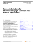
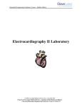
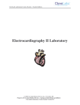
Freescale Semiconductor
Application Note
Document Number: AN4323
Rev. 0, 06/2011
Freescale Solutions for
Electrocardiograph and Heart
Rate Monitor Applications
by: Jorge González
Guadalajara, México
1
Introduction
This application note describes how to use the
MED-EKG development board, a highly efficient board
that can be connected to the Freescale Tower System to
obtain an electrocardiogram signal and measure heart
rate.
The demo can be implemented in the TWR-K53 module,
a member of the Kinetis K50 microcontroller family, or
in the Flexis MM family’s TWR-MCF51MM or
TWR-S08MM128.
This demo uses the Freescale USB stack to send data to
a PC, making it possible to monitor heart activity through
a graphical user interface (GUI).
The Tower System and MED-EKG board allow the user
to implement heart signal conditioning in three different
modes:
• With the internal OPAMPs and TRIAMPs of the
microcontrollers.
© Freescale Semiconductor, Inc., 2011. All rights reserved.
Contents
1
2
Introduction . . . . . . . . . . . . . . . . . . . . . . . . . . . . . . . . . . . 1
Heart rate and electrocardiograph fundamentals . . . . . . 2
2.1 Heart: functional description . . . . . . . . . . . . . . . . . . 2
2.2 Electrical activity of the heart. . . . . . . . . . . . . . . . . . 3
2.3 Heart signals and the QRS complex . . . . . . . . . . . . 4
2.4 Biological electrical potentials . . . . . . . . . . . . . . . . . 5
2.5 Heart rate ranges. . . . . . . . . . . . . . . . . . . . . . . . . . . 6
3
Hardware description. . . . . . . . . . . . . . . . . . . . . . . . . . . . 7
3.1 EKG system implementation . . . . . . . . . . . . . . . . . . 8
3.2 Signal acquisition. . . . . . . . . . . . . . . . . . . . . . . . . . . 9
3.3 Instrumentation amplifier . . . . . . . . . . . . . . . . . . . . 10
3.4 Filtering . . . . . . . . . . . . . . . . . . . . . . . . . . . . . . . . . 12
3.5 Digital signal controller (DSC) . . . . . . . . . . . . . . . . 15
4
Software architecture. . . . . . . . . . . . . . . . . . . . . . . . . . . 15
4.1 Freescale USB stack . . . . . . . . . . . . . . . . . . . . . . . 16
4.2 State machines . . . . . . . . . . . . . . . . . . . . . . . . . . . 18
4.3 Timer configuration and functioning . . . . . . . . . . . 18
4.4 ECG initialization . . . . . . . . . . . . . . . . . . . . . . . . . . 19
4.5 Measurement and conditioning . . . . . . . . . . . . . . . 20
5
Getting started and running the MED-EKG demo . . . . . 26
5.1 Hardware settings and connections . . . . . . . . . . . 26
5.2 Graphical user interface for the MED-EKG . . . . . . 30
6
Reference documents . . . . . . . . . . . . . . . . . . . . . . . . . . 32
Appendix A
Comparison between Freescale microcontrollers . . . . . . . . . 33
Appendix B
Communication protocol . . . . . . . . . . . . . . . . . . . . . . . . . . . . 34
Heart rate and electrocardiograph fundamentals
•
•
With the external instrumentation amplifier and operational amplifiers featured in the MED-EKG
board.
With a mixture of both.
The information in this application note is intended for developers of medical applications, for those in the
medical field, such as biomedical engineers or doctors, or for people who want to know more about the
operation of heart rate monitors and electrocardiograph devices.
2
Heart rate and electrocardiograph fundamentals
This section provides an introduction the basic concepts of heart activity in order to explain the
development of the electrocardiograph demo.
2.1
Heart: functional description
The heart is located in the middle of the thorax, positioned slightly on the left and surrounded by the lungs.
Its function is to pump blood to all parts of the body so that the organs receive oxygen.
The heart can be divided into four chambers: two upper atria (right and left) and two lower ventricles (right
and left). Atria receive blood coming, respectively from the tissues or lungs through the venous system,
and ventricles eject blood towards the tissues or lungs. Figure 1 shows the cardiac conduction system with
the structure just mentioned.
Figure 1. Cardiac conduction system
Freescale Solutions for Electrocardiograph and Heart Rate Monitor Applications, Rev. 0
2
Freescale Semiconductor
Heart rate and electrocardiograph fundamentals
The cardiac cycle is described next and complemented with Figure 2, which is a scheme of the blood flow
in the circulatory system. The cycle consists of three principal stages:
1. Atrial systole: Atria contract and throw blood to the ventricles in a passive way. Once the blood
has been expelled from the atria, atrioventricular valves (located between atria and ventricles) are
closed to avoid blood return.
2. Ventricular systole: The ventricles contract, ejecting blood towards the circulatory system. At this
stage, it is necessary to overcome the high pressure of the aortic and pulmonary valves. Ventricles
are never completely emptied, retaining some of the blood.
3. Diastole: At this point, all the parts of the heart are relaxed to allow the arrival of new blood.
Figure 2. Blood circulation scheme
2.2
Electrical activity of the heart
There is some electrical activity in the heart, related to depolarization and re-polarization of myocardial
cells, that accompanies the blood flow. This electrical activity is the source of our ability to measure the
heartbeat with electronic means. The electrical impulse starts in the sinoatrial node and flows first through
the atria, reaching the atrioventricular node and generating the atrium contraction. After that, there is a
brief pause and the current flows through the His bundle towards the ventricles, generating their
contraction. Finally, current arrives to the Purkinje fibers and repolarization of the heart tissue occurs.
The following sequence represents electrical activity during a heartbeat. It is depicted in Figure 3:
1. Atrium begins to depolarize.
Freescale Solutions for Electrocardiograph and Heart Rate Monitor Applications, Rev. 0
Freescale Semiconductor
3
Heart rate and electrocardiograph fundamentals
2.
3.
4.
5.
6.
Atrium depolarizes.
Ventricles begin to depolarize at apex. Atrium repolarizes.
Ventricles depolarize.
Ventricles begin to repolarize at apex.
Ventricles repolarize.
Figure 3. Electrical activity in myocardium
2.3
Heart signals and the QRS complex
The boxes included in Figure 3 represent voltage signals generated during heartbeat. The sequence of
pulses comprise the typical heart signal shown in Figure 4.
Figure 4. Electrocardiogram signal
Heart muscles generate different voltages in the order of hundreds of microvolts. This signal has very low
amplitude and an important amount of electrical noise. The QRS complex is usually the central and largest
part of the electrocardiogram signal. The P wave represents the atrium contraction, while the QRS
complex and T wave represent the actions of the ventricles. The higher amplitude of the QRS complex
compared with the P wave is due to the fact that the ventricles contain more muscle mass than atria.
Actually, there is one atrium repolarization wave that resembles an inverse P wave, but it is buried inside
the QRS wave. The electrocardiogram signal is really useful in diagnosing cardiac arrhythmias,
Freescale Solutions for Electrocardiograph and Heart Rate Monitor Applications, Rev. 0
4
Freescale Semiconductor
Heart rate and electrocardiograph fundamentals
conduction abnormalities, ventricular hypertrophy, myocardial infarction, electrolyte derangements, and
other heart diseases.
2.4
Biological electrical potentials
As mentioned previously, the heart generates potentials that can be expressed as vector quantities, meaning
that it is possible to assign a numeric value with its respective sign to those quantities. For the sake of
clarification, the heart could be represented as a dipole located in the thorax with a specific polarity at a
certain moment, and an inverted polarity the next moment. The potential in a specific moment depends on
the amount of charge and the separation between charges.
When we refer to potentials, we are actually talking about potential differences; therefore heart signals
must be acquired with a reference point, which is used to determine significant variations from the points
whose potentials we want to record. An example of how we can acquire signals is shown in Figure 5. This
example uses an operational amplifier, since its principal function is to obtain the potential difference
between two signals and amplify it.
Figure 5. Signal acquisition
A lead is one pair of electrodes or a combination of electrodes. In cardiology, there are three basic leads:
at 0° (Lead I), 60° (Lead II) and 120° (Lead III). Figure 6 is a representation of those leads that, together,
form an imaginary figure known as Einthoven’s Triangle.
Freescale Solutions for Electrocardiograph and Heart Rate Monitor Applications, Rev. 0
Freescale Semiconductor
5
Heart rate and electrocardiograph fundamentals
Figure 6. Einthoven’s Triangle
The three electrodes for measuring the electrical signals are placed on the limbs; one on the left arm (LA),
one on the right arm (RA), and the last on the left leg (LL). The reason for connecting electrodes that way
is to obtain the bio-potentials coming from the chest, more specifically from the heart.
2.5
Heart rate ranges
Heart rate varies depending on several factors such as age, gender, metabolism, genetics, physical
activities, temperature, and so on. One of the most common situations in which heart rate is measured is
during exercise, when an athlete wants to know how hard he or she is training.
Figure 7 correlates average heart rate with physical condition and age.
Freescale Solutions for Electrocardiograph and Heart Rate Monitor Applications, Rev. 0
6
Freescale Semiconductor
Hardware description
Figure 7. Exercise zones
3
Hardware description
When it comes to measuring heart rate or displaying an electrocardiogram, the first consideration is the
acquisition of an accurate, noiseless signal with enough amplitude to be quantified. The Kinetis K50 and
the TWR-MCF51MM and TWR-S08MM128 from Flexis MM family offer many advantages in this
regard.
The features of Kinetis K50 and some of the peripherals in its integrated measurement engine are:
• Ultra low-power operation
• 2 operational amplifiers (OPAMP)
• 2 trans-impedance amplifiers (TRIAMP)
• 2 × 12-bit DAC
• 2 × 16-bit SAR ADC, up to 31 channels with programmable gain amplifiers (PGA)
• Inter-integrated circuit (I2C)
• USB connectivity
• ARM® Cortex™ M4 core with digital signal processor (DSP) instructions
The TWR-MCF51MM and TWR-S08MM128 provide the next useful features and peripherals:
• Ultra low-power operation
• 2 operational amplifiers (OPAMP)
• 2 trans-impedance amplifiers (TRIAMP)
• 16-bit SAR analog to digital converter (ADC), 4 differential channels and up to 12 external
single-ended channels.
Freescale Solutions for Electrocardiograph and Heart Rate Monitor Applications, Rev. 0
Freescale Semiconductor
7
Hardware description
•
•
•
•
•
12-bit digital-to-analog converter (DAC)
Inter-integrated circuit (I2C)
Universal serial bus (USB) connectivity
Multiply-accumulate unit (MAC only in MCF51MM)
ColdFire V1 and HCS08 cores, respectively
In addition, the MED-EKG board counts with the MC56F8006, a 16-bit digital signal controller (DSC)
which performs the digital filtering of the signal. Main DSC features are:
• 3 analog comparators (ACMP)
• 2 x 12-bit ADC
• 6 PWM outputs
• I2C
• JTAG-ONCE for programming
The DSC communicates with the microcontroller through the I2C bus.
3.1
EKG system implementation
Figure 8 is a general block diagram of the MED-EKG system.
Freescale Solutions for Electrocardiograph and Heart Rate Monitor Applications, Rev. 0
8
Freescale Semiconductor
Hardware description
Host PC with
MED-EKG
GUI
Low-pass
filter
PWM
16-bit digital
signal controller
(MC56F8006)
I2C
ECG
ADC
DSC_ADC
External
amplifier
Electrodes
•On-board
•External
Band-pass
filter
Low-pass
filter
Low-pass
filter
External
OPAMP
Notch
filter
High-pass
filter
DAC
Instrumentation
amplifier using
internal
amplifiers
MICROCONTROLLER
Band-pass
filter
Reference
voltage
(1.6 V)
USB
MODULE
Instrumentation
amplifier
(EL8172FSZ)
Supply
voltage
(3.3 V)
Internal
OPAMP
ADC BASELINE
Internal amplifiers
In/Out
Blocks featured on the MED-EKG board
Internal blocks of MM or Kinetis microcontroller
User selectable
These stages are connected to several blocks. See SCH-26527 for reference
Optional block, digital filtering can be performed internally
Figure 8. MED-EKG system block diagram
Freescale Solutions for Electrocardiograph and Heart Rate Monitor Applications, Rev. 0
Freescale Semiconductor
9
Hardware description
3.2
Signal acquisition
The first step in obtaining a heart signal is the physical interface with human. The embedded electrodes of
the MED-EKG board are one way to achieve this. A signal can be detected just by placing the fingers of
both hands on the electrodes. Figure 9 shows the MED-EKG board with the mentioned electrodes.
Figure 9. MED-EKG development board connectors
As shown in Figure 9, a connector is provided to use external electrodes, because contact is more secure
and there is less input noise that with on-board electrodes, which are very sensitive to any small movement.
Users can either purchase a three-lead cable required for that connector or read AN4223, Connecting
Low-Cost External Electrodes to MED-EKG, available at www.freescale.com.
3.3
Instrumentation amplifier
As mentioned before, signals detected by electrodes have a low voltage in the order of hundreds of
microvolts, making the amplification of those signals necessary. An instrumentation amplifier consists of
three operational amplifiers (see Section 2.4, “Biological electrical potentials”); two of them are for
buffering input signals and the third one is for differential signal gain. This kind of amplifier has a very
high common-mode rejection ratio to eliminate noise and also counts with high accuracy, which makes it
ideal for instrumentation systems.
Users can decide to use either the integrated instrumentation amplifier or the one implemented with the
microcontroller’s internal amplifiers.
It is important to mention that reference electrodes are connected to a reference voltage, because an
acquired signal has negative values and the amplifiers used can’t drive negative output signals.
Freescale Solutions for Electrocardiograph and Heart Rate Monitor Applications, Rev. 0
10
Freescale Semiconductor
Hardware description
3.3.1
Instrumentation amplifier using internal OPAMPs
It is possible to use the internal OPAMPs and TRIAMPs of the Kinetis and MM microcontrollers to
implement an instrumentation amplifier. The connection diagram is shown in Figure 10.
Figure 10. Instrumentation amplifier with internal OPAMPs and TRIAMPs
The gain is configured with jumpers J4 and J3 of the MED-EKG board, and it has to be the same in both
cases. The equivalent gain of the amplifier is as detailed below:
Connections (J3 and J4)
1–2
2–3
Gain
G
100K
 100
1K
G
100 K
 10
10 K
The output of the amplifier is sent to a band-pass filter.
3.3.2
External instrumentation amplifier (EL8172FSZ)
The EL8172 is an instrumentation amplifier implemented as an integrated circuit (IC) whose gain is
configurable through external resistors. Figure 11 shows the use of this IC in the MED-EKG board:
Freescale Solutions for Electrocardiograph and Heart Rate Monitor Applications, Rev. 0
Freescale Semiconductor
11
Hardware description
Figure 11. Instrumentation amplifier with IC EL8172
The gain of the amplifier is determined with R33 and R32. The calculation is shown below:
 R32 
 34 K 
G 
 1  
  1  85.57
 R 33 
 402 
The digital signal controller generates a PWM signal that functions as an offset generator, with the
intention of maintaining the EKG signal variations with a base level, giving stability to the signal shown
in the GUI and resulting in a more precise heart rate measurement.
Again, the output of this amplifier is sent to the respective band-pass filter, and such output is also used by
the DSC as a reference to generate the adequate PWM feedback signal.
3.4
Filtering
Although instrumentation amplifiers have a good noise-rejection ratio, it is still necessary to filter some
noise from the signal. Some causes for noise are electric installation, muscle contractions, respiration,
electromagnetic interference, and electromagnetic emissions from electronic components. A band-pass
filter helps in attenuating those sources of noise. A low limit rejects signals caused by respiration and
muscle contractions. A high limit avoids the pass of electromagnetic high-frequency interferences.
As can be seen in the system’s block diagram, there is one band-pass filter for the internally implemented
instrumentation amplifier and another for the external. Each one has different limit frequencies; these are
described in the next section.
3.4.1
Band-pass filter (0.5 Hz – 250 Hz)
The limit frequencies for the first band-pass filter, the one located after the internal instrumentation
amplifier configuration are 0.5 and 250 Hz, correspondingly. The values for capacitors and resistors and
the correspondent process to obtain cut frequencies are described below:
• High limit (250 Hz):C = 22nF R = 29.4 K
f 
1
1

 246.06 Hz
2RC 2 ( 29.4 K)( 22nF )
Freescale Solutions for Electrocardiograph and Heart Rate Monitor Applications, Rev. 0
12
Freescale Semiconductor
Hardware description
•
Low limit (0.5 Hz): C = 0.33 F
f 
R=1M
1
1

 0.482Hz
2RC 2 (1M)(0.33uF )
Filter implementation is shown in Figure 12.
Figure 12. Band-pass filter from 0.5 Hz to 250 Hz
After band-pass filtering, an extra internal operational amplifier adjusts the signal to better levels to be sent
to the microcontroller’s ADC. Developers may configure the MED-EKG board’s J2 and J5 jumpers to
select one of the following options:
3.4.2
J2
J5
Operation
1–2
—
Negative input of the amplifier is connected directly to Vref (1.6 V) and gain is
configured by software.
2–3
1–2
2–3
Open
Amplifies the signal with a gain of 69.
Gain of the signal = 1. Amplifier acts like a buffer.
Band-pass filter (0.5 Hz – 153 Hz)
The other band-pass filter is placed at the output of the EL8172FSZ and it has cut frequencies of 0.5 and
153 Hz, respectively. The low frequency is the same as in the first filter, which was obtained in
Section 3.4.1, “Band-pass filter (0.5 Hz – 250 Hz).” We now have the math for high frequency:
High limit (153 Hz):C = 22 nF
R = 47 K
f 
1
1

 153 .9 Hz
2RC 2 ( 47 K)( 22 nF )
Freescale Solutions for Electrocardiograph and Heart Rate Monitor Applications, Rev. 0
Freescale Semiconductor
13
Hardware description
As can be seen in Figure 13, there is another external OPAMP and a low-pass filter that condition the signal
with more appropriate levels to deliver to the DSC. The low-pass filter values have already been used in a
previous filter from Section 3.4.1, “Band-pass filter (0.5 Hz – 250 Hz),” and the gain of the amplifier is
simply calculated with the following equation:
G
R35
100 K
1 
 1  20.56
R37
5.11K
Figure 13. Band-pass filter from 0.5 to 153 Hz
Resistors R25 and R26 help to maintain the offset of the band-pass filter’s input signal, since negative
values of the signal must not get lost. The output of all these blocks is finally sent to the DSC.
3.4.3
Notch filter (60 Hz)
There is an extra filter called “notch filter” that helps to eliminate a specific frequency. In this case, the
frequency is 60 Hz. The reason to include this filter is to eliminate any noise related to an electrical power
source, since electrical installations have a 60 Hz frequency. Figure 14 shows the distribution of the
components that form the notch filter. The diagram also includes two more filters and an operational
amplifier. The filters are just high- and low-pass, but with the same cut frequencies of the band-pass filter.
The amplifier provides a gain of 3.3.
Freescale Solutions for Electrocardiograph and Heart Rate Monitor Applications, Rev. 0
14
Freescale Semiconductor
Software architecture
Figure 14. Notch filter
The microcontroller uses the signal coming out of the notch filter as a reference upon which to set a base
level. The microcontroller does this by delivering a feedback signal from the output of the internal DAC
to the previously mentioned high-pass filter. Finally, the signal resulting from all these blocks is sent to the
microcontroller for sampling and measurement.
3.5
Digital signal controller (DSC)
Once the DSC receives the signal through one of its ADCs, it takes samples of the signal and makes
conversions from the analog values to digital values. These values are used to perform a digital filtering
that sends an improved signal to the microcontroller through the I2C bus. The DSC also calculates heart
rate by itself and sends the value to the MCU.
As mentioned before, the DSC also gives back a PWM signal to the circuit to establish a baseline on the
electrocardiogram.
An advantage of this DSC is that, despite the fact that it has been factory programmed for digital filtering,
it is possible to reprogram it with the external JTAG-ONCE interface, using the connector embedded in
the MED-EKG board; this way, users can program their own applications.
It is possible to avoid using the DSC, since the ARM cortex M4 (Kinetis K50) and ColdFire V1
(MCF51MM) cores can execute multiply-accumulate (MAC) DSP instructions to perform the digital
filtering internally. The HCS08 core is capable of filtering the signal even though it doesn’t have the MAC
feature, but with a loss in performance. Besides, the peripherals in the microcontroller modules can obtain
the different signals and achieve both the conversion to digital and the computation of heart rate, as well
as the offset control.
4
Software architecture
This section describes the software functions most relevant for obtaining a valid heart rate and maintaining
the signal in a stable operation baseline. It also explains some of the routines related to the ECG demo. A
notable feature of the software is that it is conformed using state machines, which offers more efficiency
by emulating parallelism.
Freescale Solutions for Electrocardiograph and Heart Rate Monitor Applications, Rev. 0
Freescale Semiconductor
15
Software architecture
NOTE
The respective software for TWR-K53N512, TWR-MCF51MM, and
TWR-S08MM128 is available on the Freescale website along with this
application note.
4.1
Freescale USB stack
The microcontroller communicates with the host PC through a USB interface. Freescale offers a solution
to implement medical applications and easily connect medical devices to the PC: Freescale’s USB stack
with personal healthcare device class (PHDC), which is a portable and easy-to-use source code designed
for many applications that require interconnection with a host computer. The USB stack makes it possible
for developers to focus only on their applications without having to worry about USB protocol. In this case,
the USB device acts like a communication device class (CDC).
The graphical user interface (GUI) installed in the host computer controls the actions of the MED-EKG
demo with a series of data packet transactions. Basically, there are three types of packets:
• REQ packet: The host sends a REQUEST packet either to start or to stop a measurement.
• CFM packet: After the device receives a REQ packet, a CONFIRMATION packet is sent to the
host in order to notify that the command is valid or that there was an error.
• IND packet: Once the buffer of the ECG with the data to be sent is full, the microcontroller sends
an INDICATION packet and the data as well.
Figure 15 is a diagram showing the basic functioning of the USB protocol, and a more detailed explanation
can be found in the appendix B, at the end of this document.
Freescale Solutions for Electrocardiograph and Heart Rate Monitor Applications, Rev. 0
16
Freescale Semiconductor
Software architecture
Serial Communication Protocol:
request received
Evaluate request
Request = start measurement
Currently
measuring?
No
Request = stop measurement
Yes
No
Currently
measuring?
No state changes
Yes
• Initialize ADCs
• State = measuring
• Start timer
• Stop timer
• State = idle
Send confirmation
Send confirmation
Continue
Serial Communication Protocol:
new data ready
Currently
measuring?
No
Yes
Continue
Copy ECG buffer to OutBuffer
Send indication and ECG data
Figure 15. Communication with host PC
Freescale Solutions for Electrocardiograph and Heart Rate Monitor Applications, Rev. 0
Freescale Semiconductor
17
Software architecture
4.2
State machines
The software for the MED-EKG includes the functionality of state machines. These state machines
provide the demo with some kind of “memory,” meaning that the device can switch from one task to
another, remembering the “state” it was in before the change, or the “next state” to be taken up. This type
of execution emulates parallelism and ensures that the process follows a well-defined sequence of steps,
or “states.” It is this state machine functionality that allows the device to send data packets, for example,
while measurement is underway. Figure 16 presents the concept of state machines in a graphical format.
State Machine A
State Machine B
Other tasks or state machines
State (1)
State (1)
Task
State (2)
State (2)
Task
State (3)
State (3)
Task
Figure 16. State machine outline
4.3
Timer configuration and functioning
The MED-EKG demo uses the timer module to generate interrupts each millisecond. One sample of the
electrocardiogram signal is taken every 2 milliseconds, meaning that two periods of the timer have to pass
between successive samples.
The timer has to be forced to generate interrupts each millisecond depending on the bus clock frequency.
Figure 17 contains a flow chart explaining the basic functioning of the timer.
Freescale Solutions for Electrocardiograph and Heart Rate Monitor Applications, Rev. 0
18
Freescale Semiconductor
Software architecture
Timer interrupt
Decrement count
Count = 0?
No
Yes
New sample = TRUE
Remove timer
Return
Figure 17. Timer events flow chart
With each interrupt generated by the timer, the interrupt routine verifies whether or not the count is over
in order to indicate that a new sample of the ECG signal can be taken. When the count is zero, the timer is
deactivated until the software starts it again.
4.4
ECG initialization
This part of the software is used to initialize the peripherals of the microcontroller used in the MED-EKG
demo. The flow chart for this stage is shown in Figure 18.
Peripherals initialization
Initialize DAC
Initialize OPAMPs
and TRIAMPs
Initialize I/O ports
Initialize ECG Timer
End
Figure 18. ECG initialization flow chart
Freescale Solutions for Electrocardiograph and Heart Rate Monitor Applications, Rev. 0
Freescale Semiconductor
19
Software architecture
4.5
Measurement and conditioning
The software described in this section is the most important of the project because it handles the ECG
signal data and calculates the heart rate as well. All this information is sent, afterwards, to a host device
using the Freescale USB stack. This block also controls the offset voltage provided by the
microcontroller’s DAC—which sets a base level for the ECG signal—and the gain for one of the internal
OPAMPs.
4.5.1
State measuring
The principal function performed by the system consists of the process depicted in Figure 19. It is one of
the possible states in the state machine and its name is “StateMeasuring.” This function is called after a
request from the host device to start ECG measurement. As the flow chart below shows, execution departs
from the function through the blocks labeled “Return.” The purpose of this is to perform some tasks related
to USB communication while waiting for another lapse to sample the signal. It is a periodic routine;
therefore, the system always comes back to it while the host device does not send a request for abortion.
The basic algorithm consists of the following:
• While the current state is “State Measuring,” the software waits for the timer interrupt routine to
indicate when a new sample of the signal must be taken.
• Once the time for a new sample has passed, the microcontroller performs two analog-to-digital
conversions; one of them is merely to adjust the baseline and the other is the ECG signal itself.
• The software calls a routine that handles the baseline adjustment. That routine is
“PerformControlAlgorithm.”
• The successive samples are compared, in order to detect when a big variation occurs, by checking
the difference between samples against a predefined threshold.
• Heart rate is calculated with each new pulse detected in the base of a counter incremented with each
sample taken between successive peaks. This value is called Real Time Heart Rate because it is
obtained immediately after the occurrence of a new pulse.
• The function “CalculateHeartRateMedian” is called to obtain a more reliable heart rate—one that
considers not only the last value but the previous ones as well.
• The heart rate calculated in the last step is stored in a buffer. When the buffer is full, the data is sent
to the PC via the communication protocol.
Freescale Solutions for Electrocardiograph and Heart Rate Monitor Applications, Rev. 0
20
Freescale Semiconductor
Software architecture
State measuring
No
New sample ready?
Yes
Return
New sample = FALSE
• Read ADC: feedback value
• Read ADC: ECG signal value
• Start timer
Control algorithm
Time without
pulses > 2.5 s
Yes
Heart rate = 0
No
Peak detected?
No
Yes
Valid pulse
conditions?
No
Return
Yes
Calculate and store new realtime heart rate in HR array
Calculate heart rate median
No
ECG buffer full?
Yes
Store current heart
rate in ECG buffer
Serial communication:
new data ready
Return
Figure 19. Measurement flow chart
Freescale Solutions for Electrocardiograph and Heart Rate Monitor Applications, Rev. 0
Freescale Semiconductor
21
Software architecture
4.5.2
Baseline acquisition
In order to provide a feedback signal and set a base level so the MED-EKG demo signal is stable on the
screen of the GUI, the microcontroller first has to obtain the current approximate offset of the signal. To
do this, the software performs an averaging algorithm that takes a certain number of samples (in this case
15), orders them, and obtains the median of the data. Afterwards, the microcontroller decides between
keeping the signal on the same level or modifying the voltage delivered to the MED-EKG board through
the DAC output. Such process correspond to the function “PerformControlAlgorithm” and can be
observed in Figure 20.
Control algorithm
Samples
count < #samples
Yes
No
Store sample in array
Samples count = 0
Return
Order data
Obtain median
Low limit <
median < high limit
Yes
No
Compensate
offset with DAC
DAC output = 1.6 V
Return
Figure 20. Baseline control flowchart
Below is a brief explanation of the algorithm:
• Each sample of the baseline signal is stored in an array.
• Once the determined quantity of samples have been stored in the array, the software orders the
values within the same array in ascending order and obtains the middle, or median, value.
• The median of the values is compared with several ranges to determine whether or not it is
necessary to change the feedback voltage and how much to change it.
Freescale Solutions for Electrocardiograph and Heart Rate Monitor Applications, Rev. 0
22
Freescale Semiconductor
Software architecture
4.5.3
Heart rate
It was already mentioned in Section 4.5.1, “State measuring,” that heart rate is calculated with each sample
of the ECG signal. That value corresponds to a real time heart rate, but it is not reliable because eventually
some pulses take less or more time to occur, and the measurement could change drastically. For this reason,
several successive heart rate indicators are averaged to obtain a more approximate value. The algorithm is
similar to the one used to obtain the baseline, but in this case the heart rate median is updated every 4 peaks,
although the last 18 pulses are considered. The algorithm corresponds to the software routine called
“CalculateHeartRateMedian,” whose flow chart is in the Figure 21.
Calculate heart rate median
Copy HR array
Order data of copy
Median counter
<4
No
Yes
Obtain median
• HR sum = HR sum + median
• Increment median counter
• Calculate average
(current heart rate)
• HR sum = 0
Return
Figure 21. Heart rate flowchart
4.5.4
Gain control
The gain control algorithm allows the user to modify the amplitude of the signal shown on the GUI by
pressing a pair of buttons featured in the tower board for each microcontroller. This action consists of
changing the gain for one of the internal OPAMPs of the microcontroller. With these buttons, it is possible
either to increase or decrease the gain of the operational amplifier so that the ECG signal is at a more
convenient level. Software dedicated to this function consists simply in polling the signals coming from
the buttons and changing the gain of the OPAMP with the appropriate register.
The following flowchart (Figure 22) depicts the gain control.
Freescale Solutions for Electrocardiograph and Heart Rate Monitor Applications, Rev. 0
Freescale Semiconductor
23
Software architecture
Gain control
SW4 pressed?
Yes
• Turn on D9
• Decrease gain
No
SW2 pressed?
Yes
• Turn on D10
• Increase gain
No
Both
SW2 and SW4
released?
No
Yes
• Turn LEDs off
End
Figure 22. Gain control flowchart
The microcontroller is continuously checking for the state of the buttons, since it is part of an infinite loop,
so the gain is updated at any time when the user presses one of the buttons.
4.5.5
Automatic gain algorithm
Automatic gain control (AGC) is an alternative to the buttons mentioned in Section 4.5.4, “Gain control.”
The algorithm consists of checking the amplitude of the ECG signal constantly to change the gain of the
internal amplifier in real time if necessary. This offers a convenient alternative to pushing a button to
maintain the signal between appropriate levels.
The basic algorithm consists of the following:
• There is a counter in the software that is incremented each time a sample of the ECG signal is taken.
This counter serves to maintain a register of the time elapsed.
• If we consider a minimum heart rate of 40 bpm, a pulse should occur at least every 1.5 seconds. A
window time of 1.2 seconds (50 bpm) is acceptable to detect a heartbeat since heart rate is generally
higher than 40 bpm.
• Within the time window, we look for the lowest and highest sample of the ECG signal by constantly
updating two registers that contain the current minimum and maximum values. Once the time
window is over, the difference between those values determines the maximum peak-to-peak
amplitude of the signal during that period.
Freescale Solutions for Electrocardiograph and Heart Rate Monitor Applications, Rev. 0
24
Freescale Semiconductor
Software architecture
•
The software checks if the amplitude value is between the proper ranges; if it is not, the gain of the
internal amplifier is changed either to increase or decrease it.
Figure 23 is a graphical representation of this algorithm.
New sample
Sample  Min
Yes
Min = sample
No
Sample  Max
Yes
No
Max = sample
End
Automatic gain control
Counter =
time window
No
Yes
Return
Amplitude = Max – MIn
Initialize Max and Min
Amplitude 
low limit
Yes
Increase gain
No
Amplitude 
high limit
No
Yes
Decrease gain
Return
Figure 23. Automatic gain control flow chart
Freescale Solutions for Electrocardiograph and Heart Rate Monitor Applications, Rev. 0
Freescale Semiconductor
25
Getting started and running the MED-EKG demo
5
Getting started and running the MED-EKG demo
So far, this application note has analyzed the general implementation and functioning of the MED-EKG
demo with the advantages of Freescale MCUs. This section explains how to use the demo with the help of
the graphical user interface (GUI). You can find the MED-EKG GUI in the same folder as the software
from Freescale’s website.
Previous sections have mentioned that the GUI communicates with the microcontroller via USB port,
using the Freescale USB stack, which performs an algorithm that creates a virtual serial port to send and
receive data. For further reference and information about Freescale USB stack with PHDC please visit
www.freescale.com.
5.1
Hardware settings and connections
The contents of this section are intended as a guide in the implementation and operation of the MED-EKG
demo. Instructions are provided for both the Kinetis K50 and Flexis MM tower modules.
5.1.1
MED-EKG demo with Kinetis K50
The following steps have to be completed in order to run the MED-EKG demo in the TWR-K53:
1. Download the software for the demo from the website. It comes with the GUI and a jumper setting
file. Install the GUI on your computer.
2. Download the IAR Embedded Workbench® from the IAR Systems® website (www.iar.com). The
Kinetis demo software was developed using this platform. Install it on your computer.
3. Assemble the tower system with the elevators, TWR-SER, TWR-K53, and the MED-EKG analog
front end. Be sure to match the primary and secondary sides of the microcontroller board with the
respective elevators.
(Refer to the jumper setting file to configure the necessary jumpers).
Freescale Solutions for Electrocardiograph and Heart Rate Monitor Applications, Rev. 0
26
Freescale Semiconductor
Getting started and running the MED-EKG demo
Figure 24. Parts of the tower to be assembled
4. Open the IAR system and search for the project in the software folder. The name is
USB_CDC.eww.
5. Connect the microcontroller board to the computer using a USB cable. The computer must
recognize the Open Source BDM debug port. Install the driver for the OSBDM in the IAR folder.
6. Verify that the selected debugger is “PE micro” in the project options panel
(Project/Options/Debugger) as shown in Figure 25.
Freescale Solutions for Electrocardiograph and Heart Rate Monitor Applications, Rev. 0
Freescale Semiconductor
27
Getting started and running the MED-EKG demo
Figure 25. Selecting appropriate debugger
7. To load the microcontroller with the project, click on the “Download and debug” icon. The IAR
screen of Figure 26 shows the location of the icon.
Figure 26. IAR screen
8. After programming the Kinetis K53, refer to Section 5.2, “Graphical user interface for the
MED-EKG,” for instructions on how to connect the electrodes and use the graphical interface.
5.1.2
MED-EKG demo with Flexis MM
The steps for the TWR-MCF51MM and the TWR-S08MM128 are listed below:
1. Download the software for the TWR-MCF51MM/TWR-S08MM128 from www.freescale.com,
unzip the folder, and install the included GUI.
Freescale Solutions for Electrocardiograph and Heart Rate Monitor Applications, Rev. 0
28
Freescale Semiconductor
Getting started and running the MED-EKG demo
2. Ensure that the host computer has CodeWarrior v6.3 and the latest service pack for MCF51MM256
(if necessary). Otherwise, download and install them.
3. Connect the modules of the tower system (elevators, TWR-SER, TWR-MCF51MM256 or
TWR-S08MM128, and the MED-EKG board). The primary and secondary elevators need to match
the corresponding sides of the microcontroller board.
Figure 27. Tower system assembled for the MED-EKG demo
4. Using the USB ports, connect the serial and microcontroller modules from the tower system to the
host computer. The first time you connect the tower to the PC, it will ask for the driver of the Open
Source BDM. You can either choose the option “Install the software automatically” or specify the
path to the driver, which is, by default: C:\Program Files\Freescale\CodeWarrior for
Microcontrollers V6.3\Drivers\Osbdm-jm60.
Figure 28. USB connections
5. Open CodeWarrior v6.3 and program the microcontroller with the “ECG for MCF51MM” or
“ECG for S08MM” project, included in the compressed folder. Figure 29 shows an example of
how to do this if you are using the TWR-MCF51MM. For the TWR-S08MM128, the target must
be “HCS08 FSL Open Source BDM.” Those options are placed in the left side of the CodeWarrior
screen.
Freescale Solutions for Electrocardiograph and Heart Rate Monitor Applications, Rev. 0
Freescale Semiconductor
29
Getting started and running the MED-EKG demo
Figure 29. CodeWarrior programming interface
6. When the microcontroller has been programmed, refer to Section 5.2, “Graphical user interface for
the MED-EKG,” for instructions about the connection of the electrodes and the graphical user
interface.
5.2
Graphical user interface for the MED-EKG
The heart signal can be monitored using the MED-EKG GUI, which shows both the signal through time
and the heart rate of the person. The GUI is shown in Figure 31, with an example of the signal displayed
when the demo is running.
Follow the steps below to perform ECG measurement:
1. Once the microcontroller is programmed and the TWR-SER module is connected to the computer
via USB, the next step is to connect the electrodes. Figure 30 is an example of the correct way to
do this. In this case, we use the Welch Allyn® ECG Lead Wires, although it is possible to use the
embedded electrodes or build your own leads, as mentioned before.
Freescale Solutions for Electrocardiograph and Heart Rate Monitor Applications, Rev. 0
30
Freescale Semiconductor
Getting started and running the MED-EKG demo
Figure 30. Electrode connection
2. Press the reset button on the microcontroller board. When the demo is used for the first time, you
have to install the driver for the USB CDC Virtual COM. The default path for the driver is:
c:\Program Files\Freescale\MED-EKG\Driver\.
3. Go to the device manager in Windows and search for the port assigned to the USB CDC Virtual
COM. This port assignment is requested by the GUI.
4. Open the Graphical User Interface: Start > All programs > Freescale MED-EKG.
5. Select the appropriate COM port number from the list displayed in the menu located on the upper
right side of the GUI.
6. Press the start button. The ECG signal will start being displayed. Wait for the signal to stabilize.
You can see the electrocardiogram signal and the heart rate as well.
Freescale Solutions for Electrocardiograph and Heart Rate Monitor Applications, Rev. 0
Freescale Semiconductor
31
Reference documents
Figure 31. MED-EKG GUI
6
Reference documents
In addition to this application note, the following documents are available at www.freescale.com:
• Reference manuals and data sheets for Kinetis K53 (K53P144M100SF2RM, K53P144M100SF2),
MCF51MM256 (MCF51MM256RM, MCF51MM256), and MC9S08MM128
(MC9S08MM128RM, MC9S08MM128).
• MED-EKG board User Manual (MED-EKGUG).
• Schematics of the Tower Modules and MED-EKG board.
• Quick Start Guides.
• USB Stack with PHDC User Guide (MEDUSBUG).
Freescale Solutions for Electrocardiograph and Heart Rate Monitor Applications, Rev. 0
32
Freescale Semiconductor
Comparison between Freescale microcontrollers
Appendix A
Comparison between Freescale microcontrollers
The demo described in this document has been implemented with three microcontrollers: the
MCF51MM256, the MC9S08MM128, and the Kinetis K50. Table A-1 is a brief comparative analysis of
those MCUs.
Table A-1. Freescale MCU comparison
Characteristic
MC9S08MM128
MCF51MM256
Kinetis K50
Core
HCS08 (8-bit)
48 MHz Core
24 MHz Bus
ColdFire V1 with MAC
8–32 bit compatibility
50.33 MHz Core
25.165 MHz Bus
ARM Cortex-M4
with MAC DSP+SIMD
72 MHz or 100 MHz
Flash / SRAM
128 KB Flash
12 KB RAM
256 KB Flash
32 KB RAM
64–512 KB Flash
64–128 KB RAM
A/D converter
16-bit SAR ADC
16-bit SAR ADC
2 × 16-bit SAR ADC
D/A converter
12-bit DAC
12-bit DAC
2 × 12-bit DAC
Timers
2 × 4 channel, TPM with
PWM
2 × 4 channel, TPM with
PWM
3 × 12 channel Timer
Communication
Interfaces
2 × SCI
2 × SPI
USB Device
I2C
2 × SCI
2 × SPI
USB Device/Host/OTG
I2C
MiniFlexBus
6 x SCI
3 × SPI
USB OTG
Ethernet
Secure Digital Host Controller
(SDHC)
FlexBus
Other
PRACMP
2 × OPAMP
2 × TRIAMP
PRACMP
2 × OPAMP
2 × TRIAMP
3 × ACMP
2 × OPAMP
2 × TRIAMP
2 × Programmable Gain
Amplifier (PGA)
Random Number Generator
(RNG)
LCD Driver
Touch Sensing Interface
Freescale Solutions for Electrocardiograph and Heart Rate Monitor Applications, Rev. 0
Freescale Semiconductor
33
Communication protocol
Appendix B
Communication protocol
The application communicates with the GUI on the PC using the Freescale USB Stack with PHDC, with
the device acting as a communication device class (CDC). The device communicates via a serial interface
similar to the RS232 communications standard but emulating a virtual COM port.
Once the device has been connected and a proper driver has been installed, the PC will recognize it as a
Virtual COM Port and it will be accessible, for example using HyperTerminal. Communication is
established using the following parameters.
Bits per second: 115200
Data bits: 8
Parity: None
Stop Bits: 1
Flow Control: None
Communication starts when the host (PC) sends a request packet indicating to the device the action to
perform. The device then responds with a confirmation packet indicating to the host that the command has
been received. At this point, the host must be prepared to receive data packets from the device and show
the data received on the GUI. Communication finishes when the host sends a request packet indicating that
the device should stop. The following block diagram describes the data flow.
Figure B-1. Communication protocol data flow
Freescale Solutions for Electrocardiograph and Heart Rate Monitor Applications, Rev. 0
34
Freescale Semiconductor
Communication protocol
Packets sent between host and device have a specific structure. Each packet is divided into four main parts:
packet type, command opcode, data length, and the data itself. The image below shows the packet
structure.
Figure B-2. Packet structure
Packet Type
The packet type byte defines the kind of packet to be sent. There are three kinds of packets that can be sent
between host and device.
REQ packet: This is a request packet. This kind of packet is used by the host to request the device to
perform some action, such as starting or stopping a measurement. A REQ packet is usually composed of
2 bytes: packet type and command opcode. Data length and data packet bytes are not required.
CFM packet: This is a confirmation packet. This kind of packet is used by the device to confirm to the
host that a command has been received. It sends a response indicating whether the command is accepted
or if the device is busy.
IND packet: This is an indication packet. This kind of packet is used to indicate to the host that an event
has occurred in the device and data needs to be sent. This is used, for example, when the device has a new
set of data to be sent to the GUI.
The following table shows the respective HEX codes for each packet type.
Packet Type
HEX Code
REQ
0x52
CFM
0x43
IND
0x69
Command Opcode
The command opcode byte indicates the action to be performed for a REQ packet and the kind of
confirmation or indication in case of CFM and IND packet types, respectively. There are different opcodes
for each packet type. The following table shows the different opcodes.
NOTE
Software related with this application note does not respond to all of these
commands.
Freescale Solutions for Electrocardiograph and Heart Rate Monitor Applications, Rev. 0
Freescale Semiconductor
35
Communication protocol
Opcode
IND
Opcode
(Hex)
REQ
CFM
GLU_START_MEASUREMENT
X
X
0x00
GLU_ABORT_MEASUREMENT
X
X
0x01
GLU_START_CALIBRATION
X
X
0x02
Glucose Meter
GLU_BLOOD_DETECTED
X
0x03
GLU_MEASUREMENT_COMPLETE_OK
X
0x04
GLU_CALIBRATION_COMPLETE_OK
X
0x05
Blood Pressure Meter
BPM_START_MEASUREMENT
X
X
0x06
BPM_ABORT_MEASUREMENT
X
X
0x07
BPM_MEASUREMENT_COMPLETE_OK
X
0x08
BPM_MEASUREMENT_ERROR
X
0x09
BPM_START_LEAK_TEST
X
X
0x0A
BPM_ABORT_LEAK_TEST
X
X
0x0B
BPM_LEAK_TEST_COMPLETE
X
0x0C
BPM_SEND_PRESSURE_VALUE_TO_PC
X
0x28
Electro Cardiograph Opcode
ECG_HEART_RATE_START_MEASUREMENT
X
X
0x0D
ECG_HEART_RATE_ABORT_MEASUREMENT
X
X
0x0E
ECG_HEART_RATE_MEASUREMENT_COMPLETE_OK
X
0x0F
ECG_HEART_RATE_MEASUREMENT_ERROR
X
0x10
ECG_DIAGNOSTIC_MODE_START_MEASUREMENT
X
X
0x12
ECG_DIAGNOSTIC_MODE_STOP_MEASUREMENT
X
X
0x13
ECG_DIAGNOSTIC_MODE_NEW_DATA_READY
X
0x14
Thermometer
TMP_READ_TEMEPRATURE
X
X
0x15
X
X
0x16
X
X
0x17
Height scale
HGT_READ_HEIGHT
Weight scale
WGT_READ_WEIGHT
Spirometer
Freescale Solutions for Electrocardiograph and Heart Rate Monitor Applications, Rev. 0
36
Freescale Semiconductor
Communication protocol
Opcode
CFM
SPR_DIAGNOSTIC_MODE_START_MEASURMENT
X
X
0x1C
SPR_DIAGNOSTIC_MODE_STOP_MEASURMENT
X
X
0x1D
SPR_DIAGNOSTIC_MODE_NEW_DATA_READY
IND
Opcode
(Hex)
REQ
X
0x1E
Pulse Oximetry
POX_START_MEASURMENT
X
X
0x21
POX_ABORT_MEASURMENT
X
X
0x22
POX_MEASURMENT_COMPLETE_OK
X
0x23
POX_MEASURMENT_ERROR
X
0x24
POX_DIAGNOSTIC_MODE_START_MEASURMENT
X
X
0x25
POX_DIAGNOSTIC_MODE _STOP_MEASURMENT
X
X
0x26
POX_DIAGNOSTIC_MODE_NEW_DATA_READY
X
0x27
0x21
System commands
SYS_CHECK_DEVICE_CONNECTION
X
SYS_RESTART_SYSTEM
X
X
0x29
0x2A
Data Length and Data String
The data length and data string bytes are the data quantity count and the data itself. In other words the data
length byte represents the number of bytes contained in the data string. The data string is the information
to be sent, just the data; therefore, the data length byte must not count the packet type byte, the command
opcode byte, or itself.
Functional Description
Communication starts when the host sends a REQ packet indicating that the device should start a new
measurement. The host must send a REQ packet type to start transactions (Figure B-3).
Figure B-3. Start packet sent by host
The start opcode can be any opcode related with start a measurement. For example, if we wanted to start
ECG in diagnostic mode, the data packet will look like Figure B-4.
Figure B-4. Starting ECG in diagnostic mode
Freescale Solutions for Electrocardiograph and Heart Rate Monitor Applications, Rev. 0
Freescale Semiconductor
37
Communication protocol
0x52 is the HEX code for a REQ packet type; 0x12 corresponds to
ECG_DIAGNOSTIC_MODE_START_MEASUREMENT. After sending the REQ packet, a CFM packet
must be received indicating the status of the device. The received packet must look like Figure B-5.
Figure B-5. Confirmation packet structure
The error byte will indicate the device status. The table below shows the possible error codes.
Error
HEX Code
OK
0x00
BUSY
0x01
INVALID OPCODE
0x02
If the error byte received corresponds to OK, the device will start sending data as soon as a new data packet
is ready. If a BUSY error is received, the host must try to communicate later. If error received is INVALID
OPCODE, data sent and transmission lines must be checked.
If a CFM packet with an OK error has been received, the device will start sending information related to
the requested measurement. This is performed using indication packets (IND). The indication packet
structure is shown in Figure B-6.
Figure B-6. Indication packet structure
The first byte contains the respective HEX code for an indication packet type. The second byte contains
the opcode for the kind of indication. For example, if the device is sending an indication packet for
ECG_DIAGNOSTIC_MODE_NEW_DATA_READY, the HEX code read in this position will be 0X14
since this is the indication opcode for a new set of data from ECG diagnostic mode. The next byte is the
length, which indicates the quantity of data to be sent.
The first couple of bytes after the length byte are the packet ID bytes. The packet ID is a 16-bit data divided
into 2 bytes to be sent. It contains the number of packets to be sent. The packet ID number of a data packet
is the packet ID of the previous packet + 1. For example, if the packet ID of the previous packet sent was
0X0009, the packet ID of the next packet must be 0x000A. This allows the GUI to determine if a packet
is missing.
The following data bytes are the data string; they contain the information of the requested measurement.
Data quantity is determined by the data length byte and data is interpreted depending on the kind of
measurement specified. For example, for MED-EKG demo, Data 2 to Data n-1 contains the data to be
graphed. Each point on the graph is represented by a 16-bit signed number. This means that each of the 2
data bytes in the packet is one point in the graph. The first byte is the most significant part of the long (16
bits) and the second byte is the less significant part. The sign of the long data is set using one’s
complement. The last byte contains the heart rate measurement. This byte must be taken as it is an
Freescale Solutions for Electrocardiograph and Heart Rate Monitor Applications, Rev. 0
38
Freescale Semiconductor
Communication protocol
unsigned char data that contains the number of beats per minute. Figure B-7 shows a typical MED-EKG
demo indication packet.
Figure B-7. MED-EKG IND packet
When a stop request is sent by the host, the device stops sending data and waits for a new start request
command. Table B-8 shows the stop command structure.
Figure B-8. Stop command structure
Immediately after this, the device must acknowledge with a CFM packet like the shown in Figure B-9.
Figure B-9. Stop CFM packet
The CFM packet for stop does not require an error code; it only has to be received. If this packet has not
been received, the request has been rejected or not taken and must be sent again in order to stop the
measurements.
Freescale Solutions for Electrocardiograph and Heart Rate Monitor Applications, Rev. 0
Freescale Semiconductor
39
How to Reach Us:
Home Page:
www.freescale.com
Web Support:
http://www.freescale.com/support
USA/Europe or Locations Not Listed:
Freescale Semiconductor, Inc.
Technical Information Center, EL516
2100 East Elliot Road
Tempe, Arizona 85284
+1-800-521-6274 or +1-480-768-2130
www.freescale.com/support
Europe, Middle East, and Africa:
Freescale Halbleiter Deutschland GmbH
Technical Information Center
Schatzbogen 7
81829 Muenchen, Germany
+44 1296 380 456 (English)
+46 8 52200080 (English)
+49 89 92103 559 (German)
+33 1 69 35 48 48 (French)
www.freescale.com/support
Japan:
Freescale Semiconductor Japan Ltd.
Headquarters
ARCO Tower 15F
1-8-1, Shimo-Meguro, Meguro-ku,
Tokyo 153-0064
Japan
0120 191014 or +81 3 5437 9125
[email protected]
Asia/Pacific:
Freescale Semiconductor China Ltd.
Exchange Building 23F
No. 118 Jianguo Road
Chaoyang District
Beijing 100022
China
+86 10 5879 8000
[email protected]
For Literature Requests Only:
Freescale Semiconductor Literature Distribution Center
1-800-441-2447 or 303-675-2140
Fax: 303-675-2150
[email protected]
Document Number: AN4323
Rev. 0
06/2011
Information in this document is provided solely to enable system and software
implementers to use Freescale Semiconductor products. There are no express or
implied copyright licenses granted hereunder to design or fabricate any integrated
circuits or integrated circuits based on the information in this document.
Freescale Semiconductor reserves the right to make changes without further notice to
any products herein. Freescale Semiconductor makes no warranty, representation or
guarantee regarding the suitability of its products for any particular purpose, nor does
Freescale Semiconductor assume any liability arising out of the application or use of any
product or circuit, and specifically disclaims any and all liability, including without
limitation consequential or incidental damages. “Typical” parameters that may be
provided in Freescale Semiconductor data sheets and/or specifications can and do vary
in different applications and actual performance may vary over time. All operating
parameters, including “Typicals”, must be validated for each customer application by
customer’s technical experts. Freescale Semiconductor does not convey any license
under its patent rights nor the rights of others. Freescale Semiconductor products are
not designed, intended, or authorized for use as components in systems intended for
surgical implant into the body, or other applications intended to support or sustain life,
or for any other application in which the failure of the Freescale Semiconductor product
could create a situation where personal injury or death may occur. Should Buyer
purchase or use Freescale Semiconductor products for any such unintended or
unauthorized application, Buyer shall indemnify and hold Freescale Semiconductor and
its officers, employees, subsidiaries, affiliates, and distributors harmless against all
claims, costs, damages, and expenses, and reasonable attorney fees arising out of,
directly or indirectly, any claim of personal injury or death associated with such
unintended or unauthorized use, even if such claim alleges that Freescale
Semiconductor was negligent regarding the design or manufacture of the part.
For information on Freescale’s Environmental Products program, go to
http://www.freescale.com/epp.
Freescale™ and the Freescale logo are trademarks of Freescale Semiconductor, Inc.
All other product or service names are the property of their respective owners.
The Power Architecture and Power.org word marks and the Power and Power.org logos
and related marks are trademarks and service marks licensed by Power.org. ARM®
Cortex™ M4 is the registered trademark of ARM Limited.
© Freescale Semiconductor, Inc. 2011. All rights reserved.