Download Electrocardiography II Laboratory

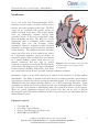
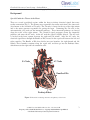
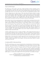
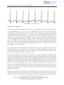
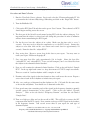
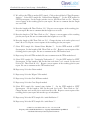
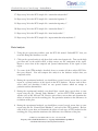
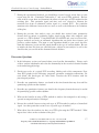
CleveLabs Laboratory Course System – Student Edition
Electrocardiography II Laboratory
2006 Cleveland Medical Devices Inc., Cleveland, OH.
Property of Cleveland Medical Devices. Copying and distribution prohibited.
CleveLabs Laboratory Course System Version 6.0
CleveLabs Laboratory Course System – Student Edition
Electrocardiography II Laboratory
Introduction
As we saw in the first electrocardiography (ECG)
laboratory session, surface electrodes can be used to
measure the cardiac potential in the heart. The ECG
signal can be correlated with specific regions of
cardiac excitation in the heart. The cardiac rhythm
relies on synchronous electrical activity from
specialized tissues of the heart to effectively pump
blood throughout the body. The ECG has several
applications such as evaluating cardiac function,
calculating heart rate, and detecting cardiac
arrhythmias. However, sometimes cardiac electrical
activation can become irregular and cause abnormal
cardiac function. The abnormal electrical activation
can be caused by areas of dead cardiac tissue caused
by a myocardial infarction, extra pace makers, or
congenital defects. When the heart does not contract
in a normal rhythmic pattern, blood does not get
pumped effectively and may lead to several
symptoms in a person or even death. The ECG can be Figure 1. Atria and ventricles of the heart with
blood flow patterns (red-oxygenated, blue –
used to detect and diagnose several types of abnormal deoxygenated).
cardiac function including bradycardia (slow heart
rate), tachycardia (fast heart rate), and other electrical conduction problems.
Quantitative features of the ECG signal can be analyzed and correlated to specific cardiac
abnormalities. The ability to quantify and classify the type of cardiac event that a person may be
experiencing is critical for properly treating the abnormal rhythm. For example, many cardiac
defibrillators and pace makers currently include a set of ECG monitoring electrodes. Smart
algorithms are included in the devices that detect the type of arrhythmia that is occurring. If the
type of cardiac event warrants a defibrillating shock, the system then delivers it to the patient.
There are several quantitative temporal and spectral tools that can be used to analyze
physiological signals that will be introduced in this session and may be used throughout the rest
of this laboratory course.
Equipment required:
•
•
•
•
CleveLabs Kit
CleveLabs Course Software
Four (4) Snap Electrodes and Snap Leads
MATLAB® or LabVIEW™
2006 Cleveland Medical Devices Inc., Cleveland, OH.
Property of Cleveland Medical Devices. Copying and distribution prohibited.
CleveLabs Laboratory Course System Version 6.0
2
CleveLabs Laboratory Course System – Student Edition
Electrocardiography II Laboratory
Background
Special Conductive Tissues in the Heart
There are several specialized regions within the heart to initiate electrical signals that cause
cardiac contraction (Fig 2). The primary area responsible for cardiac activation is the sinus node
(also known as the sinoatrial or SA node). The SA node is located at the top of the right atrium
and is the major structure responsible for pacing the heart. Connecting the SA node to the
atrioventricular (AV) node are the internodal pathways. These internodal pathways are located
along the walls of the right atrium. The electrical signal propagates down the internodal
pathways and enters the AV node. At the AV node the signal is slightly delayed. The AV node
is located in the heart septum, between the right and left atrium. After the AV node, the
electrical signal flows through the Bundle of His, located in the septal wall between the left and
right ventricles. The Bundle of His then divides into two branches, the right branch and left
branch. These branches continue along the septal wall, and then go into the Purkinje fibers,
which innervate the right and left ventricular walls.
SA Node
AV Node
Bundle of His
Perkinje Fibers
Figure 2: Electrical conducting structures and pathways of the heart
2006 Cleveland Medical Devices Inc., Cleveland, OH.
Property of Cleveland Medical Devices. Copying and distribution prohibited.
CleveLabs Laboratory Course System Version 6.0
3
CleveLabs Laboratory Course System – Student Edition
Electrocardiography II Laboratory
Origin of the ECG Signal
In normal cases, the SA node is the heart’s natural pacemaker with the autonomic nervous
system regulating its excitation. Pulses from the SA node propagate via the internodal fibers of
the right atrium, and then to the left atrium, causing immediate atrial contraction. This electrical
potential then travels to the AV node. At the AV node, the depolarization potential is then
delayed, allowing the atria to fully contract. This delay allows the atrium to empty its contents
into the ventricles before ventricular contraction. After the delay in the AV node, the potential
travels down the Bundle of His, which splits into right and left branch bundles. These bundles
innervate the ventricular walls via the Purkinje fibers. When the signal reaches the Purkinje
fibers, ventricular contraction occurs sending blood from the right ventricle into the lungs and
blood from the left ventricle out the aorta. This process repeats for each heartbeat.
Other cardiac tissues also have natural pacing rates controlled by the autonomic nervous system.
The AV node, without outside stimulation, has a natural discharge rate of 40 to 60 times a
minute, while the Purkinje fibers fire between 15 and 40 times a minute. This is in contrast to
the SA node that fires between 70 and 80 times a minute. Neither the AV node nor the Purkinje
fibers are responsible for setting the heart rate due to the discharge rate of the SA node. The SA
node fires fastest, so other tissues are excited from the SA impulse rather than their own. In
normal conditions, the SA node is the natural pacemaker of the heart. However, sometimes the
AV node or Purkinje fibers begin pacing faster than the SA node. This condition is known as an
ectopic pacemaker. An ectopic pacemaker occurs when electrical activation of the heart is
initiated elsewhere than the SA node.
Another condition that can lead to an ectopic pacemaker is when signals from the SA node are
prevented from conducting to the rest of the heart. This may occur when the electrical impulses
are blocked at the AV node or AV fibers that innervate the ventricles. In this instance, the SA
node fires at its own normal rate, but the signals do not conduct down to the ventricles. Since the
Purkinje fibers do not receive these impulses from the SA node, they begin to fire at their own
intrinsic rate, between 15-40 times a second. This leads to a very slow contraction rate of the
ventricles, failing to pump blood. If this continues, the brain may become deprived of oxygen,
and the person may faint.
Correlation of ECG to Physiological Events
The ECG signal illustrates the electrical depolarization and repolarization of the heart during a
contraction. As described above, the depolarization of the cardiac muscle cells in the atrium
occurs first. Therefore, the first wave in the ECG signal corresponds to the depolarization of the
atrium. This is known as the P wave. Similarly, the start of ventricular contraction is the QRS
wave. The ventricles stay contracted for a few milliseconds until ventricular repolarization
occurs, which is seen as the T wave. Atrial repolarization typically occurs between 0.15 and 0.20
seconds after the P wave. However, this is the same time when the QRS complex occurs. The
QRS complex is of much greater amplitude than atrial repolarization so it dominates the signal.
2006 Cleveland Medical Devices Inc., Cleveland, OH.
Property of Cleveland Medical Devices. Copying and distribution prohibited.
CleveLabs Laboratory Course System Version 6.0
4
CleveLabs Laboratory Course System – Student Edition
Electrocardiography II Laboratory
Figure 3. Normal ECG signal.
Abnormalities in the ECG
As stated previously, ECG recordings can be used as a diagnostic tool to determine abnormalities
in cardiac function, or it can be used to visualize the effects of cardiac tissue damage.
Abnormalities in the QRS complex indicate problems in the ventricles or ventricular conduction.
A normal QRS complex lasts between .6 -.8 seconds. Times longer than this indicate a change in
ventricular conduction. One cause is ventricular dilation, or hypertrophy. In this case, the
ventricles are larger than normal, causing the impulse to take longer to conduct through the
tissue, elongating the QRS complex. In these cases, the QRS might last between 0.9 to 0.12
seconds. Another cause for lengthened QRS complexes are conduction blocks in the Purkinje
fibers. As described above, these fibers conduct the impulse from the Bundle of His node into
the ventricles. If a complete block of the Purkinje fibers occurs, the QRS complex can be
lengthened to .14 seconds or more.
Conduction from the SA node can also be blocked. In this case, the signal from the SA node is
blocked before it ever reaches the atria, causing the sudden disappearance of the P wave,
meaning the atria fail to contract. Since the ventricular tissues have their own rhythm, the AV
node creates the QRS-T complex, but at a slower rate.
Blocks and conduction delays can also be found in the AV node. One type of block that comes
from AV conduction problems is indicated by an elongated P-R (or P-Q) interval. The normal
time from the beginning of the P wave until the beginning of the QRS complex is 0.16 seconds.
A first-degree block occurs when that time is greater than 0.20 seconds. In first-degree block, the
QRS is delayed, but not actually blocked. When the PR interval begins to grow longer to 0.25 to
0.30 seconds, some impulses may not be strong enough to pass through the AV node. This leads
to dropped beats where the QRS complex disappears, even though there is a preceding P wave.
These cases are called second-degree block. A second-degree block can cause the heart to
develop an asynchronous 2:1 rhythm. In this case, there are 2 atrial contractions for each
ventricular contraction.
Third degree block occurs when the signal from the SA node never reaches the ventricles due to
complete block of the AV node. In this case, the ventricles never receive the cardiac impulses
and begin to beat at their own natural rate, which is much slower than the rate from the SA node.
2006 Cleveland Medical Devices Inc., Cleveland, OH.
Property of Cleveland Medical Devices. Copying and distribution prohibited.
CleveLabs Laboratory Course System Version 6.0
5
CleveLabs Laboratory Course System – Student Edition
Electrocardiography II Laboratory
Consequently, the relation between P waves and QRS complexes disappear. The P wave will be
regular, but QRS-T complexes will appear at a much slower rate.
In a normal ECG, the T wave is of positive amplitude, denoting the repolarization of the
ventricles. In some abnormal ECG, the T wave can be inverted, having negative amplitude. One
reason for this is slow conduction of the depolarization wave. In this instance, the conduction
delay occurs in the left ventricle due to a left bundle branch block. Consequently, the right
ventricle depolarizes first, then the left ventricle depolarizes, causing a shift of the mean QRS
vector to the left. Then, as repolarization occurs, the right ventricle repolarizes before the left
ventricle, causing the mean axis for the T wave to shift to the right, which is opposite of the QRS
complex in the same measurement. So, with delay of the conduction of the depolarization wave
in the ventricles, the inversion of the T wave occurs. Another cause for inverted T waves is
delayed depolarization. In this case, repolarization does not occur at the same place as it
normally does. Instead, repolarization occurs at the apex of the heart. Delayed depolarization
causes the base of the ventricles to repolarize before the apex, causing the vector to point from
the apex to the base of the ventricles, which is opposite to the repolarization vector in normal
cases, inverting the T wave. The most likely cause for this type of depolarization delay is mild
ischemia of the heart tissue, which can be caused by coronary occlusion or coronary
insufficiency that may occur during exercise.
Coronary ischemia caused either by myocardial infarction or other damage to the heart muscle
can cause changes to the ECG signal. Since ischemia means a loss of blood flow to the muscle
tissue, there is a loss of nutrients due to decreased blood flow, a lack of oxygen, and a buildup of
carbon dioxide. Consequently, ischemic cardiac muscle is unable to repolarize, and remains
depolarized so long as the muscle is ischemic. Since this muscle remains depolarized at all times,
current flows between this injured depolarized muscle and the normal polarized areas during the
cardiac cycle. This is known as a current of injury. When cardiac tissue is consistently
depolarized, it affects the ECG by causing a deflection in the graph due to a strong current of
injury. Using vector analysis, a physician can use the ECG to determine the location of this
ischemic tissue by looking at the polarity of the current of injury.
Abnormal rhythms can be analyzed using ECG recordings. Rhythm disorders, such as
tachycardia and bradycardia are quite evident. Tachycardia is when the heart rate exceeds 100
beats per minute, and is usually caused by increased body temperature, stimulation by the
sympathetic nervous system, or chemical stimulation of the heart tissue. Bradycardia is when the
heart rate slows to less than 60 beats per minute. Bradycardia is not always harmful. Some
athletes demonstrate bradycardia due to the fact that their heart has become extremely efficient at
pumping blood. This reduces the need for a faster heart rate. But bradycardia can also be a result
of vagal stimulation, which has an inhibitory effect on heart rate. A description of several other
cardiac arrhythmias is listed below:
Atrial Fibrillation
2006 Cleveland Medical Devices Inc., Cleveland, OH.
Property of Cleveland Medical Devices. Copying and distribution prohibited.
CleveLabs Laboratory Course System Version 6.0
6
CleveLabs Laboratory Course System – Student Edition
Electrocardiography II Laboratory
The most common type of sustained arrhythmia is atrial fibrillation (AF), which occurs as a
result of rapid, irregular electrical impulses stimulating the atria. This prevents the atria from
contracting normally, though blood can continue to flow passively through the atria. Some
common causes include heart lesions that prevent the atria from emptying adequately into the
ventricles and ventricular failure that causes excess damming of blood in the atria. These
conditions cause dilated atrial walls, which make the heart susceptible to the long conduction
pathways and slow conduction that can result in AF. The frequent, irregular waves stimulating
the atria are weak and often of opposite polarity, which results in either no P-waves or a high
frequency, low-voltage wavy ECG recording. The QRS-T complexes are normal but irregular as
a result of impulses arriving at the AV node irregularly. Heart failure and valvular heart disease
are both associated with AF.
Atrial Flutter
Atrial flutter is a condition where there are multiple atrial contractions for every ventricular
contraction. It is caused by a single large electrical signal that propagates around the atria. The
rate of atrial contraction can be between 200 and 350 beats per minute. The amount of blood
being pumped by the atria can be very small as a result of one side of the atria being contracted
while the other is being relaxed. The electrical signals enter the AV node at a rate that is too
rapid to create a ventricular contraction for every atrial contraction. As a result, there are
multiples P-waves in the ECG for every QRS-T complex.
Sinus Bradycardia
2006 Cleveland Medical Devices Inc., Cleveland, OH.
Property of Cleveland Medical Devices. Copying and distribution prohibited.
CleveLabs Laboratory Course System Version 6.0
7
CleveLabs Laboratory Course System – Student Edition
Electrocardiography II Laboratory
Bradycardia is a term to describe the heart beating more slowly than normal. Sinus bradycardia
can occur in well-conditioned athletes and during deep relaxation. In the case of athletes, the
heart muscle is tremendously strong and efficient at pumping blood, therefore, less contractions
are needed. During deep relaxation, the body is at rest and requires less oxygen consumption
than during normal activity which allows the heart rate to slow. Therefore, it may be perfectly
normal. However, sinus bradycardia can also occur as a result of heart disease or as a reaction to
medication.
Supraventricular Tachyarrhythmia
Supraventricular tachyarrhythmias (SVT) can occur in patients of all ages. This arrhythmia
consists of fast heart rates that occur in the atria or the AV junctional tissue area. However, SVT
can be a strong predictor of mortality in patients with congestive heart failure. Some examples of
this arrhythmia can include atrial flutter, Wolf-Parkinson-White syndrome (a short circuit
between the atria and ventricles), and atrial fibrillation are all examples.
Ventricular Tachycardia
2006 Cleveland Medical Devices Inc., Cleveland, OH.
Property of Cleveland Medical Devices. Copying and distribution prohibited.
CleveLabs Laboratory Course System Version 6.0
8
CleveLabs Laboratory Course System – Student Edition
Electrocardiography II Laboratory
Ventricular tachycardia is a life-threatening condition that results from electrical impulses arising
from the ventricles instead of the SA node. This results in an abnormally rapid heartbeat. Heart
attacks, cardiomyopathy, and valvular heart disease are a few of the causes of ventricular
tachycardia. The formation of scar tissue from previous heart attacks can predispose a person to
this condition. Because of the rapid heart rate, the ventricles are unable to completely fill with
blood and less blood is pumped to the rest of the body. Ventricular tachycardia can result in
heart failure, ventricular fibrillation, and cardiac arrest.
Ventricular Bigeminy
Ventricular bigeminy occurs when there is a premature beat every other beat. The premature
beat is broad, occurs earlier than normal, and is followed by a compensatory pause. Premature
beats are caused by an irritable focus of cardiac tissue in the ventricles that may result in early
depolarization of the ventricles.
Ventricular Trigeminy
2006 Cleveland Medical Devices Inc., Cleveland, OH.
Property of Cleveland Medical Devices. Copying and distribution prohibited.
CleveLabs Laboratory Course System Version 6.0
9
CleveLabs Laboratory Course System – Student Edition
Electrocardiography II Laboratory
Ventricular trigeminy occurs when there is a premature beat every third beat. The premature
beat has a widened QRS complex, occurs earlier than normal, and is followed by a compensatory
pause. Premature beats are caused by an irritable focus of cardiac tissue in the ventricles that
may result in early depolarization of the ventricles.
Ventricular Flutter
In this cardiac arrhythmia, the verticals can be paced at more than 200 beats per second. This
can be triggered by an extrasystole, or ectopic pacemaker, that occurs in the ventricles. The
pumping of blood becomes extremely inefficient. There is no visible P wave in the ECG
recording and the QRS complex and T wave are merged in regularly occurring waves with a
frequency between 180 and 250 beats per minute.
Several examples of all the abnormal cardiac arrhythmias described above are included
with the laboratory course software. You will explore these in this laboratory session.
These data files were obtained from the Physionet website at www.physionet.org.
2006 Cleveland Medical Devices Inc., Cleveland, OH.
Property of Cleveland Medical Devices. Copying and distribution prohibited.
CleveLabs Laboratory Course System Version 6.0
10
CleveLabs Laboratory Course System – Student Edition
Electrocardiography II Laboratory
Cardiac Defibrillators
In some cases, a cardiac arrhythmia can drive the cardiac output down to almost zero and create
a life threatening condition. In these cases, a cardiac defibrillator can be used to shock the heart
out of an abnormal cardiac rhythm. In general, a large electrical shock may reestablish a normal
cardiac rhythm. Current is passed though electrodes that are placed either directly on the heart or
transthoracically using large area surface electrodes placed against the chest.
Two basic types of defibrillators include capacitive-discharge and rectangular wave. The
capacitive-discharge DC defibrillators produce a short high amplitude pulse. Approximately 50
to 100 J is required for defibrillation using electrodes applied directly to the heart. External
electrodes can require up to 400 J for defibrillation. Electrodes should have excellent contact
with the body. If good contact is not maintained, energy intended to reach the heart can be
dissipated at the electrode skin interface and cause serious burns. Electrodes should also be well
insulated to prevent current from flowing through the person applying the defibrillation.
Electrocardiography Analysis Methods
As explained above and as you will see in lab course software examples, there are several types
of cardiac arrhythmias. The most effective treatment depends upon which type of arrhythmia a
person is experiencing. The types of treatment can range from nothing to pharmaceutical
interventions, to implanting electrical pacemakers, to cardiac defibrillation. Therefore, it is
important to identify which type of abnormality exists. One method for accomplishing this is
through a visual inspection of the ECG signals by a trained clinician. As explained above, there
are several visual features that can be extracted to detect which cardiac event is occurring.
However, a physician is not always readily available to review these recordings. Therefore, it
may be advantageous to use a computer based program to quantitatively assess the ECG signal
and classify it as a particular rhythm. These intelligent algorithms can be integrated into medical
devices such as implanted cardiac pace makers and cardiac defibrillators.
Several tools are available to provide quantitative analysis of temporal and spectral components
of the cardiac signal. In addition, this laboratory session will introduce a joint time-frequency
analysis (JFTA). This method allows users to analyze signals in both the time and frequency
domains simultaneously (Fig 4). It is a useful tool to analyze non-stationary signals. Essentially,
this method yields which frequencies are occurring at what times. A normal ECG signal can be a
fairly stationary signal. However, an abnormal cardiac signal can become non-stationary in
which case this method may be appropriate to analyze the signal. A graphical representation
illustrates how the signal power spectrum changes over time. The basic approach is to divide the
signal into several discrete intervals that can be overlapped. A Fourier transform can then be
applied to each block of data to illustrate the frequency components of each block. The size of
the discrete intervals determines the time accuracy. In other words, the smaller the discrete
block of time is, the better the time resolution. However, there is a tradeoff to this method. The
frequency resolution is inversely proportional to the time resolution. This is known as the
2006 Cleveland Medical Devices Inc., Cleveland, OH.
Property of Cleveland Medical Devices. Copying and distribution prohibited.
CleveLabs Laboratory Course System Version 6.0
11
CleveLabs Laboratory Course System – Student Edition
Electrocardiography II Laboratory
window effect. The smaller the discrete interval of time, the less resolution of frequency is
provided. The algorithm described above is known as a short-time Fourier transform (STFT).
Figure 4. A joint time-frequency analysis can be useful for analyzing many physiological signals including the
cardiac potential.
Other algorithms that can be used in the JFTA method include an adaptive spectrogram, a ChoiWilliams distribution, a Cone-shaped distribution, Wigner-Ville distribution, and the Gabor
spectrum. Each algorithm has a unique impact on the time and frequency resolutions that can be
achieved, cross-term interference, and computational speed. The Gabor algorithm expands the
signal into a set of weighted frequency-modulated Gaussian functions and is the inverse of the
STFT. It has good time and frequency resolution and the speed of the algorithm is moderate.
The Wigner-Ville distribution gives high time and frequency resolution but suffers from cross
term interference. This algorithm is computationally fast and does not suffer from windowing
effects. The Cohen’s class algorithms such as the Choi-Willimas, and Cone shaped distributions
act to reduce this crossterm interference. Both algorithms provide good time and frequency
response, but computationally they are very slow. The appropriate method to use is based on the
particular application at hand.
Experimental Methods
Experimental Setup
During this laboratory you will record a standard three lead ECG. You should watch the setup
movie included with the software prior to setting up the experiment.
1. Your BioRadio should be programmed to the “LabECGII” configuration.
2006 Cleveland Medical Devices Inc., Cleveland, OH.
Property of Cleveland Medical Devices. Copying and distribution prohibited.
CleveLabs Laboratory Course System Version 6.0
12
CleveLabs Laboratory Course System – Student Edition
Electrocardiography II Laboratory
Figure 5: Setup for Lab ECG II.
2. For this laboratory you will use four snap electrodes from the CleveLabs Kit. Remember
that the electrode needs to have good contact with the skin to get a high quality recording.
The surface of the skin should be prepared and cleaned prior to electrode placement. For
the best recordings, it is best to mildly abrade the surface with pumice or equivalent to
minimize contact resistance by removing the outer dry skin layer. Attach one electrode
on the palmar side of the right wrist, one on the palmar side of the left wrist, one on the
left leg, and one on the right leg. NOTE: The electrodes on the arms can be placed at
the wrists and the electrodes on the legs can be placed near the ankles.
3. After the electrodes have been placed on the subject, connect one snap lead to each of the
four electrodes. Then, connect those snap leads to the harness inputs channels 1, 2, 3,
references, and the ground using the picture above as a reference (Fig 5). The leads on
the harness are stackable allowing one snap lead to be plugged into more than one
connector lead.
2006 Cleveland Medical Devices Inc., Cleveland, OH.
Property of Cleveland Medical Devices. Copying and distribution prohibited.
CleveLabs Laboratory Course System Version 6.0
13
CleveLabs Laboratory Course System – Student Edition
Electrocardiography II Laboratory
Procedure and Data Collection
1. Run the CleveLabs Course software. Log in and select the “Electrocardiography II” lab
session under the Advanced Physiology subheading and click on the “Begin Lab” button.
2. Turn the BioRadio ON.
3. Click on the ECG data Tab and then on the green “Start” button. Three channels of ECG
should begin scrolling across the screen.
4. The first part of the lab will record normal resting ECG with the subject sitting up. It is
important that the subject is relaxed and still during this procedure in order to minimize
artifacts from contaminating the ECG signal.
5. For the first test, have the subject sit in a chair. Make sure the time scale is set to 3
seconds. You may need to adjust the amplitudes to see the ECG clearly. Instruct the
subject to relax then click on the save button and record data for approximately 10
seconds. Name the data file “subjectECG1”.
6. Stop saving data. Report a screen shot of this data to your report. You may want to
name your report “Electrocardiography II”.
7. Save two more data files each approximately 10s in length. Name the data files
“subjectECG2” and “subjectECG3”. Later you will compare your 3 saved data files from
the subject to the abnormal clinical database.
8. Now we will examine the abnormal clinical database. Click on the tab labeled “Sample
ECG”. In the top right hand corner is a drop down menu of 27 ECG sample waveforms.
There are a total of 9 cardiac rhythms with 3 examples of each.
9. Examine each of the signals in the time domain as they scroll across the screen. Report a
screen shot of each of the 9 rhythms to include into your report.
10. Also, save each type of abnormal cardiac rhythm to a file. Call each file the same name
as the cardiac arrhythmia. You should save 8 abnormal cardiac files.
11. Now spend some time examining each of the signals in the frequency domain to quantify
specific spectral characteristics of the signals. Click on the tab labeled “Spectral
Analysis”. Click on the tab labeled “Frequency Domain” and then the tab labeled
“Sample Data”.
12. Turn on a high pass filter and set the cut off to 0.01. This will help to remove the DC
component from the ECG signals. Now examine each type of ECG signal in the database
in the frequency domain. Add several screen shots to your report for each type of
abnormal rhythm.
2006 Cleveland Medical Devices Inc., Cleveland, OH.
14
Property of Cleveland Medical Devices. Copying and distribution prohibited.
CleveLabs Laboratory Course System Version 6.0
CleveLabs Laboratory Course System – Student Edition
Electrocardiography II Laboratory
13. We will use the JTFA to analyze ECG signals. Click on the tab labeled “Time-Frequency
Analysis”. Select ECG sample file “Normal Sinus Rhythm 3”. Set the JFTF method to
STFT Spectrogram. Set the length (window size) to 360. Then Click on “Go”. Report a
screen capture of the resulting plot for your report. Be sure to comment that the length
was set to 360.
14. Reset the length to 60. Then Click on “Go”. Report a screen capture of the resulting plot
for your report. Be sure to comment that the length was set to 60.
15. Reset the length to 720. Then Click on “Go”. Report a screen capture of the resulting
plot for your report. Be sure to comment that the length was set to 720.
16. Reset the length to 360. Then Click on “Go”. Change the time scale on the plot to read
from 2.0s to 2.5s. Report a screen capture of the resulting plot for your report.
17. Select ECG sample file “Normal Sinus Rhythm 3”. Set the JFTF method to STFT
Spectrogram. Set the length to 360. Then Click on “Go”. Report a screen capture of the
resulting plot for your report. Be sure to comment on the JTFA method used.
18. Repeat step 16 for all JTFA methods. Be sure to comment on the JTFA method used.
19. Select ECG sample file “Ventricular Tachycardia 2”. Set the JFTF method to STFT
Spectrogram. Set the length to 360. Set the time scale from 7 to 9 seconds. Set the trend
level to 0.1. Then Click on “Go”. Report a screen capture of the resulting plot for your
report. Be sure to comment on the JTFA method used.
20. Repeat step 19 for the Gabor method.
21. Repeat step 19 for the Wigner Ville method.
22. Repeat step 19 for the Choi-Williams method.
23. Repeat step 19 for the Cone Shaped method.
24. Select ECG sample file “normal sinus rhythm 1”. Set the JFTF method to STFT
Spectrogram. Set the length to 360. Set the trend level to 0.1. Then Click on “Go”.
Change the time scale on the plot to read from 10s to 20s. Report a screen capture of the
resulting plot for your report and note the type of arrhythmia.
25. Repeat step 24 for the ECG sample file “atrial fibrillation 1”.
26. Repeat step 24 for the ECG sample file “atrial flutter 3”.
2006 Cleveland Medical Devices Inc., Cleveland, OH.
Property of Cleveland Medical Devices. Copying and distribution prohibited.
CleveLabs Laboratory Course System Version 6.0
15
CleveLabs Laboratory Course System – Student Edition
Electrocardiography II Laboratory
27. Repeat step 24 for the ECG sample file “ventricular tachycardia 3”.
28. Repeat step 24 for the ECG sample file “ventricular bigeminy 1”.
29. Repeat step 24 for the ECG sample file “ventricular trigeminy 1”.
30. Repeat step 24 for the ECG sample file “ventricular flutter 3”.
31. Repeat step 24 for the ECG sample file “sinus bradycardia 1”.
32. Repeat step 24 for the ECG sample file “supraventricular tachyarrythmia 1”.
Data Analysis
1. Using the post processing toolbox, open the ECG file named “SubjectECG1” that you
recorded during this laboratory session.
2. Click on the spectral analysis tab, then click on the time domain tab. Turn on the high
pass filter and set the cutoff to 0.01 to help remove any DC component of the signal.
Report a screen shot of the temporal and spectral characteristics of the signal to your
report.
3. Use some of the JTFA methods described above to examine all three subject ECG files
that you collected. You will compare this analysis to the database analysis that you
completed earlier.
4. During the experimental methods you should have created several screen shots to your
report of a spectral analysis of the signals in the ECG database. Review each of these
screen shots and determine if there are any spectral features which are unique to
particular cardiac abnormalities.
5. During the experimental methods you should have created three screen shots to your
report using the file “Normal Sinus Rhythm 3” and the STFT JTFA methods with
window sizes of 60, 360, and 720. Review each of these screen shots and determine the
effects of window size on the resulting plot. Pay particular attention to the differences in
resolutions of the plots.
6. During the experimental methods you should have created several screen shots to your
report using the file “Normal Sinus Rhythm 3” and each of the JTFA methods. Review
each of these screen shots and determine the effects of each type of JTFA method on the
resulting plot. Pay particular attention to the differences in resolutions of the plots.
2006 Cleveland Medical Devices Inc., Cleveland, OH.
Property of Cleveland Medical Devices. Copying and distribution prohibited.
CleveLabs Laboratory Course System Version 6.0
16
CleveLabs Laboratory Course System – Student Edition
Electrocardiography II Laboratory
7. During the experimental methods you should have created several screen shots to your
report using the file “Ventricular Tachycardia 2” and several JTFA methods. Review
each of these screen shots and determine the effects of each type of JTFA method on the
resulting plot. This particular signal and time scale was selected to illustrate the
transition area from an abnormal cardiac signal to a normal ECG. Pay particular
attention to the difference between the two areas as well as the differences in resolutions
of the plots.
8. During the previous data analysis steps you should have noticed some quantitative
features that are unique to particular cardiac signals using either only temporal, only
spectral, or a JTFA method. Using MATLAB or LabVIEW and your saved data files,
propose methods and write an automated algorithm that can detect these features and
predict a cardiac rhythm. The input to your algorithm should be your saved data files
from this laboratory session and the output should be the type of cardiac rhythm. Be sure
to include the data files that you collected from a subject in your analysis as well as the
data files that you saved from the abnormal clinical database.
Discussion Questions
1. In this laboratory session you learned about several cardiac abnormalities. Discuss each
of these cardiac arrhythmias and relate the abnormality in the recorded electrical rhythm
to the underlying physiology.
2. Sketch two cycles of a typical ECG recording, labeling each of the components. Now
draw ECG graphs for the following symptoms: premature ventricular contractions, SA
node block, and first-degree AV node block. Correlate the ECG sketches with the
physiological problem.
3. Describe any quantitative features you found in the time domain that may be useful for
quantifying specific cardiac rhythms.
4. Describe any quantitative features you found in the frequency domain that may be useful
for quantifying specific cardiac rhythms.
5. What are the benefits of using a JFTA method to analyze data compared to only using a
spectral or temporal analysis technique?
6. Discuss the tradeoffs between using each type of JFTA method to analyze a biomedical
signal. Are there particular reasons to use a specific type of method?
7. What effect does the window size have on a JTFA plot using the STFT method? What
impact does it have on the resolution of the plot?
2006 Cleveland Medical Devices Inc., Cleveland, OH.
Property of Cleveland Medical Devices. Copying and distribution prohibited.
CleveLabs Laboratory Course System Version 6.0
17
CleveLabs Laboratory Course System – Student Edition
Electrocardiography II Laboratory
8. You should have designed an automated algorithm to detect particular cardiac
arrhythmias based on quantitative features of the signal. Describe in detail the methods
that you used to create this algorithm. Discuss any difficulties that you had in designing
these algorithms. Which arrhythmias could you successfully identify?
2006 Cleveland Medical Devices Inc., Cleveland, OH.
Property of Cleveland Medical Devices. Copying and distribution prohibited.
CleveLabs Laboratory Course System Version 6.0
18
CleveLabs Laboratory Course System – Student Edition
Electrocardiography II Laboratory
References
1. Webster, John G. Medical Instrumentation, Application and Design, 3rd Edition, John Wiley
and Sons, New York, 1998.
2. Guyton and Hall. Textbook of Medical Physiology, 9th Edition, Saunders, Philadelphia,
1996.
3. Normann, Richard A. Principles of Bioinstrumentation, John Wiley and Sons, New York,
1988.
4. Rhoades, R and Pflanzer, R.
Publishing, Fort Worth 1996.
Human Physiology.
Third Edition.
Saunders College
5. Goldberger AL, Amaral LAN, Glass L, Hausdorff JM, Ivanov PCh, Mark RG, Mietus JE,
Moody GB, Peng CK, Stanley HE. PhysioBank, PhysioToolkit, and PhysioNet: Components
of a New Research Resource for Complex Physiologic Signals. Circulation 101(23):e215e220
[Circulation
Electronic
Pages;
http://circ.ahajournals.org/cgi/content/full/101/23/e215]; 2000 (June 13).
6. National Instruments Corporation. Signal Processing Toolset User’s Manual. December
2002 Edition.
2006 Cleveland Medical Devices Inc., Cleveland, OH.
Property of Cleveland Medical Devices. Copying and distribution prohibited.
CleveLabs Laboratory Course System Version 6.0
19