Download Creative computing 1: image, sound and motion

Creative computing I:
image, sound and motion
Volume 1
M. Casey with
T. Taylor, A. Smaill and C. Brownrigg
CO1112
2014
Undergraduate study in
Computing and related programmes
This is an extract from a subject guide for an undergraduate course offered as part of the
University of London International Programmes in Computing. Materials for these programmes
are developed by academics at Goldsmiths.
For more information, see: www.londoninternational.ac.uk
This subject guide was prepared for the University of London International Programmes by:
Michael Casey, Department of Music, Dartmouth College, USA
Tim Taylor, Department of Computing, Goldsmiths, University of London, UK
Alan Smaill, School of Informatics, University of Edinburgh, UK
Chris Brownrigg, freelance artist and writer, UK
Additional help with production was provided by:
Sarah Rauchas, Department of Computing, Goldsmiths, University of London
This is one of a series of subject guides published by the University. We regret that due to pressure of
work the authors are unable to enter into any correspondence relating to, or arising from, the guide.
If you have any comments on this subject guide, favourable or unfavourable, please use the form at
the back of this guide.
First published 2007
This edition published 2014
University of London International Programmes
Publications Office
32 Russell Square
London WC1B 5DN
United Kingdom
www.londoninternational.ac.uk
Published by: University of London
© University of London 2014
The University of London asserts copyright over all material in this subject guide except where
otherwise indicated. All rights reserved. No part of this work may be reproduced in any form, or
by any means, without permission in writing from the publisher. We make every effort to respect
copyright. If you think we have inadvertently used your copyright material, please let us know.
Contents
Preface
v
1 History of Mathematics and Computing in Creativity
1.1 Introduction . . . . . . . . . . . . . . . . . . . . . .
1.2 Earliest Mathematics . . . . . . . . . . . . . . . . .
1.3 Ancient Greece . . . . . . . . . . . . . . . . . . . .
1.4 Arab Mathematics and Computation . . . . . . . .
1.5 The Renaissance: Geometry and Perspective . . .
1.6 Inventing Computational Thinking . . . . . . . . .
1.7 Mathematics and Music . . . . . . . . . . . . . . .
1.8 Some notes on additional reading . . . . . . . . . .
1.9 Summary and learning outcomes . . . . . . . . . .
1.10 Exercises . . . . . . . . . . . . . . . . . . . . . . . .
.
.
.
.
.
.
.
.
.
.
.
.
.
.
.
.
.
.
.
.
.
.
.
.
.
.
.
.
.
.
.
.
.
.
.
.
.
.
.
.
.
.
.
.
.
.
.
.
.
.
.
.
.
.
.
.
.
.
.
.
.
.
.
.
.
.
.
.
.
.
.
.
.
.
.
.
.
.
.
.
.
.
.
.
.
.
.
.
.
.
.
.
.
.
.
.
.
.
.
.
.
.
.
.
.
.
.
.
.
.
.
.
.
.
.
.
.
.
.
.
1
1
2
3
3
4
5
7
8
9
9
2 The Bauhaus
2.1 Background . . . . . . . . . . . . . . . . . .
2.2 The Beginning of the Bauhaus . . . . . . . .
2.2.1 Principles for the Bauhaus . . . . . .
2.3 Bauhaus developments with new staff . . .
2.4 Movement towards Constructivism . . . .
2.5 The last phase of the Bauhaus in Germany .
2.6 Summary and learning outcomes . . . . . .
2.7 Exercises . . . . . . . . . . . . . . . . . . . .
2.8 The structure of the rest of this guide . . . .
.
.
.
.
.
.
.
.
.
.
.
.
.
.
.
.
.
.
.
.
.
.
.
.
.
.
.
.
.
.
.
.
.
.
.
.
.
.
.
.
.
.
.
.
.
.
.
.
.
.
.
.
.
.
.
.
.
.
.
.
.
.
.
.
.
.
.
.
.
.
.
.
.
.
.
.
.
.
.
.
.
.
.
.
.
.
.
.
.
.
.
.
.
.
.
.
.
.
.
.
.
.
.
.
.
.
.
.
.
.
.
.
.
.
.
.
.
.
.
.
.
.
.
.
.
.
.
.
.
.
.
.
.
.
.
.
.
.
.
.
.
.
.
.
11
11
13
13
13
15
18
18
18
19
3 Introduction to Processing
3.1 Processing . . . . . . . . . . . . . .
3.2 Installing Processing . . . . . . . .
3.3 A Quick Tour of Processing . . . .
3.4 Code examples . . . . . . . . . .
3.5 Summary and learning outcomes
3.6 Exercises . . . . . . . . . . . . . .
.
.
.
.
.
.
.
.
.
.
.
.
.
.
.
.
.
.
.
.
.
.
.
.
.
.
.
.
.
.
.
.
.
.
.
.
.
.
.
.
.
.
.
.
.
.
.
.
.
.
.
.
.
.
.
.
.
.
.
.
.
.
.
.
.
.
.
.
.
.
.
.
.
.
.
.
.
.
.
.
.
.
.
.
.
.
.
.
.
.
.
.
.
.
.
.
.
.
.
.
.
.
.
.
.
.
.
.
.
.
.
.
.
.
.
.
.
.
.
.
.
.
.
.
.
.
21
21
22
23
23
24
24
4 Origins
4.1 Introduction . . . . . . . . . . . . . .
4.2 The Processing display window . . .
4.3 size() . . . . . . . . . . . . . . . . .
4.4 background() . . . . . . . . . . . . .
4.5 Coordinates . . . . . . . . . . . . . .
4.5.1 Cartesian Coordinate System
4.6 The Origin . . . . . . . . . . . . . . .
4.7 Plane Geometry . . . . . . . . . . . .
4.7.1 point() . . . . . . . . . . . .
4.8 Lines . . . . . . . . . . . . . . . . . .
4.8.1 Zero-Based Indexing . . . . .
4.9 Size of a pixel . . . . . . . . . . . . .
4.10 Summary and learning outcomes . .
4.11 Exercises . . . . . . . . . . . . . . . .
.
.
.
.
.
.
.
.
.
.
.
.
.
.
.
.
.
.
.
.
.
.
.
.
.
.
.
.
.
.
.
.
.
.
.
.
.
.
.
.
.
.
.
.
.
.
.
.
.
.
.
.
.
.
.
.
.
.
.
.
.
.
.
.
.
.
.
.
.
.
.
.
.
.
.
.
.
.
.
.
.
.
.
.
.
.
.
.
.
.
.
.
.
.
.
.
.
.
.
.
.
.
.
.
.
.
.
.
.
.
.
.
.
.
.
.
.
.
.
.
.
.
.
.
.
.
.
.
.
.
.
.
.
.
.
.
.
.
.
.
.
.
.
.
.
.
.
.
.
.
.
.
.
.
.
.
.
.
.
.
.
.
.
.
.
.
.
.
.
.
.
.
.
.
.
.
.
.
.
.
.
.
.
.
.
.
.
.
.
.
.
.
.
.
.
.
.
.
.
.
.
.
.
.
.
.
.
.
.
.
.
.
.
.
.
.
.
.
.
.
.
.
.
.
.
.
.
.
.
.
.
.
.
.
.
.
.
.
.
.
.
.
.
.
.
.
.
.
.
.
.
.
.
.
.
.
.
.
.
.
.
.
.
.
.
.
.
.
.
.
.
.
.
.
.
.
.
.
.
.
27
27
27
29
31
32
32
32
33
33
35
36
36
40
41
.
.
.
.
.
.
i
Creative Computing I: Image, Sound, Motion
5 background(), stroke() and line()
5.1 Introduction . . . . . . . . . . . . . . . . . . . .
5.2 line() . . . . . . . . . . . . . . . . . . . . . . .
5.2.1 Vertical, Horizontal and Diagonal Lines
5.2.2 background() . . . . . . . . . . . . . . .
5.2.3 stroke() . . . . . . . . . . . . . . . . . .
5.2.4 strokeWeight() . . . . . . . . . . . . .
5.2.5 Many lines . . . . . . . . . . . . . . . . .
5.2.6 strokeCap() . . . . . . . . . . . . . . .
5.3 Snap To Grid . . . . . . . . . . . . . . . . . . . .
5.4 Observing and Drawing . . . . . . . . . . . . .
5.5 Observation and practice . . . . . . . . . . . . .
5.6 Summary and learning outcomes . . . . . . . .
5.7 Exercises . . . . . . . . . . . . . . . . . . . . . .
.
.
.
.
.
.
.
.
.
.
.
.
.
.
.
.
.
.
.
.
.
.
.
.
.
.
.
.
.
.
.
.
.
.
.
.
.
.
.
.
.
.
.
.
.
.
.
.
.
.
.
.
.
.
.
.
.
.
.
.
.
.
.
.
.
43
43
43
44
45
45
45
47
47
48
48
51
52
55
6 Shape
6.1 Introduction . . . . . . . . . . . . . . . . . . . . . . . . . . . . . .
6.2 Unit Forms . . . . . . . . . . . . . . . . . . . . . . . . . . . . . . .
6.3 Construction of Simple Polygons . . . . . . . . . . . . . . . . . .
6.3.1 rect() . . . . . . . . . . . . . . . . . . . . . . . . . . . . .
6.3.2 ellipse() . . . . . . . . . . . . . . . . . . . . . . . . . . .
6.3.3 arc() . . . . . . . . . . . . . . . . . . . . . . . . . . . . . .
6.3.4 Construction of Regular Polygons using Turtle Graphics
6.3.5 Construction of Irregular Polygons . . . . . . . . . . . . .
6.4 Summary and learning outcomes . . . . . . . . . . . . . . . . . .
6.5 Exercises . . . . . . . . . . . . . . . . . . . . . . . . . . . . . . . .
.
.
.
.
.
.
.
.
.
.
.
.
.
.
.
.
.
.
.
.
.
.
.
.
.
.
.
.
.
.
.
.
.
.
.
.
.
.
.
.
57
57
57
57
58
59
60
60
63
64
65
7 Structure
7.1 Introduction . . . . . . . . . . . . . . . . . . . . . . .
7.2 Gestalt Principles . . . . . . . . . . . . . . . . . . . .
7.2.1 Proximity . . . . . . . . . . . . . . . . . . . .
7.2.2 Similarity . . . . . . . . . . . . . . . . . . . .
7.2.3 Closure . . . . . . . . . . . . . . . . . . . . . .
7.3 Interrelationship of Unit Forms . . . . . . . . . . . .
7.3.1 Disjoint . . . . . . . . . . . . . . . . . . . . . .
7.3.2 Proximal . . . . . . . . . . . . . . . . . . . . .
7.3.3 Overlapping . . . . . . . . . . . . . . . . . . .
7.3.4 Conjoined . . . . . . . . . . . . . . . . . . . .
7.4 Logical Combination . . . . . . . . . . . . . . . . . .
7.4.1 A brief introduction to colour representation
7.4.2 Bitwise logical operations on colour values .
7.4.3 Or . . . . . . . . . . . . . . . . . . . . . . . . .
7.4.4 And . . . . . . . . . . . . . . . . . . . . . . . .
7.4.5 Exclusive Or (XOR) . . . . . . . . . . . . . . .
7.4.6 Not (Inversion) . . . . . . . . . . . . . . . . .
7.5 Repetition . . . . . . . . . . . . . . . . . . . . . . . .
7.5.1 Rows . . . . . . . . . . . . . . . . . . . . . . .
7.5.2 Columns . . . . . . . . . . . . . . . . . . . . .
7.5.3 Diagonals . . . . . . . . . . . . . . . . . . . .
7.6 Recursion . . . . . . . . . . . . . . . . . . . . . . . . .
7.7 Summary and learning outcomes . . . . . . . . . . .
7.8 Exercises . . . . . . . . . . . . . . . . . . . . . . . . .
.
.
.
.
.
.
.
.
.
.
.
.
.
.
.
.
.
.
.
.
.
.
.
.
.
.
.
.
.
.
.
.
.
.
.
.
.
.
.
.
.
.
.
.
.
.
.
.
.
.
.
.
.
.
.
.
.
.
.
.
.
.
.
.
.
.
.
.
.
.
.
.
.
.
.
.
.
.
.
.
.
.
.
.
.
.
.
.
.
.
.
.
.
.
.
.
67
67
67
69
69
70
71
71
72
72
73
73
73
74
74
75
75
76
79
79
79
80
80
83
84
.
.
.
.
.
.
.
.
.
.
.
.
.
.
.
.
.
.
.
.
.
.
.
.
.
.
.
.
.
.
.
.
.
.
.
.
.
.
.
.
.
.
.
.
.
.
.
.
.
.
.
.
.
.
.
.
.
.
.
.
.
.
.
.
.
.
.
.
.
.
.
.
.
.
.
.
.
.
.
.
.
.
.
.
.
.
.
.
.
.
.
.
.
.
.
.
.
.
.
.
.
.
.
.
.
.
.
.
.
.
.
.
.
.
.
.
.
.
.
.
.
.
.
.
.
.
.
.
.
.
.
.
.
.
.
.
.
.
.
.
.
.
.
.
.
.
.
.
.
.
.
.
.
.
.
.
.
.
.
.
.
.
.
.
.
.
.
.
.
.
.
.
.
.
.
.
.
.
.
.
.
.
.
.
.
.
.
.
.
.
.
.
.
.
.
.
.
.
.
.
.
.
.
.
.
.
.
.
.
.
.
.
.
.
.
.
.
.
.
.
.
.
.
.
.
.
.
.
.
.
.
.
.
.
.
.
.
.
.
.
.
.
.
.
.
.
.
.
.
.
.
.
.
.
.
.
.
.
.
.
.
.
.
.
.
.
.
.
.
.
.
.
.
.
.
.
.
.
.
.
.
.
.
.
.
8 Motion
85
8.1 Introduction . . . . . . . . . . . . . . . . . . . . . . . . . . . . . . . . . . 85
ii
8.2
8.3
8.4
8.5
8.6
8.7
8.8
setup() and draw() . . . . . . . . . . .
Persistence . . . . . . . . . . . . . . . . .
Velocity . . . . . . . . . . . . . . . . . . .
Motion by Coordinate Transformations
Reflection at Boundaries . . . . . . . . .
Interaction . . . . . . . . . . . . . . . . .
Gravity and Acceleration . . . . . . . . .
8.8.1 Rotation and Acceleration . . . .
8.9 Random Motion . . . . . . . . . . . . . .
8.9.1 Brownian Motion . . . . . . . . .
8.9.2 Perlin Noise . . . . . . . . . . . .
8.10 Motion of Multiple Objects . . . . . . . .
8.11 Summary and learning outcomes . . . .
8.12 Exercises . . . . . . . . . . . . . . . . . .
9 Cellular Automata in 1D and 2D
9.1 Introduction . . . . . . . . . . . . . .
9.2 Bits and Pixels . . . . . . . . . . . . .
9.3 Images out of Bits . . . . . . . . . . .
9.4 Three-bit 1D Cellular Automata . . .
9.5 Two-dimensional Cellular Automata
9.5.1 Conway’s Game of Life . . .
9.6 Summary and learning outcomes . .
9.7 Exercises . . . . . . . . . . . . . . . .
9.8 Looking forward . . . . . . . . . . .
.
.
.
.
.
.
.
.
.
.
.
.
.
.
.
.
.
.
.
.
.
.
.
.
.
.
.
.
.
.
.
.
.
.
.
.
.
.
.
.
.
.
.
.
.
.
.
.
.
.
.
.
.
.
.
.
.
.
.
.
.
.
.
.
.
.
.
.
.
.
.
.
.
.
.
.
.
.
.
.
.
.
.
.
.
.
.
.
.
.
.
.
.
.
.
.
.
.
.
.
.
.
.
.
.
.
.
.
.
.
.
.
.
.
.
.
.
.
.
.
.
.
.
.
.
.
.
.
.
.
.
.
.
.
.
.
.
.
.
.
.
.
.
.
.
.
.
.
.
.
.
.
.
.
.
.
.
.
.
.
.
.
.
.
.
.
.
.
.
.
.
.
.
.
.
.
.
.
.
.
.
.
.
.
.
.
.
.
.
.
.
.
.
.
.
.
.
.
.
.
.
.
.
.
.
.
.
.
.
.
.
.
.
.
.
.
.
.
.
.
.
.
.
.
.
.
.
.
.
.
.
.
.
.
.
.
.
.
.
.
.
.
.
.
.
.
.
.
.
.
.
.
.
.
.
.
.
.
.
.
.
.
.
.
.
.
.
.
.
.
85
86
87
87
88
89
90
90
93
93
94
95
97
97
.
.
.
.
.
.
.
.
.
.
.
.
.
.
.
.
.
.
.
.
.
.
.
.
.
.
.
.
.
.
.
.
.
.
.
.
.
.
.
.
.
.
.
.
.
.
.
.
.
.
.
.
.
.
.
.
.
.
.
.
.
.
.
.
.
.
.
.
.
.
.
.
.
.
.
.
.
.
.
.
.
.
.
.
.
.
.
.
.
.
.
.
.
.
.
.
.
.
.
.
.
.
.
.
.
.
.
.
.
.
.
.
.
.
.
.
.
.
.
.
.
.
.
.
.
.
.
.
.
.
.
.
.
.
.
.
.
.
.
.
.
.
.
.
.
.
.
.
.
.
.
.
.
.
.
.
.
.
.
.
.
.
99
99
99
100
101
103
103
105
105
106
iii
Creative Computing I: Image, Sound, Motion
iv
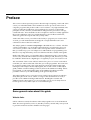
Preface
This course is about expressing creative ideas through computing. At the end of the
course you will understand some foundational creative processes in the form of
computer programs that produce audio-visual content to very high standards. The
course provides the foundations of programming for creativity coupled with
principles of form, structure, transformation and generative processes for image,
sound and video. These methods are the conceptual tools that are widely applied in
the creative industries. They are used by designers, special effects technicians,
animators, games developers and video jockeys alike.
At the end of this course you will have the facility to program your creative ideas.
As such, you will understand more deeply the concepts behind creative and
commercial software that is in wide use.
The subject guide for Creative Computing I is divided into two volumes. The first
volume will introduce you to the basic materials that you will need to start your
own creative portfolio. The second volume will expand on these foundations so
that you can develop your own unique tools and methods via programming. It is
therefore very important that you become familiar with the contents of this guide.
By the end of this course, you should be able to implement creative concepts that
are not easily realised with commercial software packages and, therefore, you will
be enabled to demonstrate a high degree of originality in your own creative work.
The assessment of this course will be formed of two pieces of course work and an
exam that you will sit at the end of the first year of the programme. The exam will
be an unseen written exam. The exam questions will be about the background,
techniques and examples in this subject guide, the second volume of this subject
guide, and the essential reading (see below) but not the additional reading. While
not required, you should read the items on the additional reading list where
possible to increase your understanding of the general subject area.
This subject guide is not a course text. It sets out the logical sequence in which to
study the topics in the course. Where coverage in the essential texts is weak, it
provides some additional background material. Reading the essential and
additional texts is important as you are expected to see an area of study from an
holistic point of view, and not just as a set of limited topics.
Some general notes about this guide
Website links
Unless otherwise stated, all websites in this subject guide were accessed in March
2014. We cannot guarantee, however, that they will stay current and you may need
to perform an internet search to find the relevant pages.
v
Creative Computing I: Image, Sound, Motion
Colour
A colour version of this subject guide is available as a PDF document in the CO1112
Creative Computing I section of the VLE.1 You may find the colour version easier to
follow.
1 http://computing.elearning.london.ac.uk
vi
Essential reading
Reas, C. and B. Fry Processing: A Programming Handbook for Visual Designers and Artists
(MIT Press, 2007) [ISBN 0262182629].
Reas, C. and B. Fry www.processing.org/reference, on-line Processing reference manual.
http://www.bauhaus.de (site available in German and English)
http://www-history.mcs.st-andrews.ac.uk/index.html
Additional reading
Bayer, H., W. Gropius and I. Gropius (eds) Bauhaus 1919-1928 (Museum of Modern Art,
1976) [ISBN 0810960133].
Behrens, R. R. Art, Design and Gestalt Theory, Leonardo, Vol. 31, No. 4, pp. 299–303, 1998.
Bell, E.T. Men of Mathematics (Simon & Schuster, 1986) [ISBN 0671628186].
Berger, J. Ways of Seeing (Penguin, reprint edition, 1990) [ISBN 0140135154].
Borchardt-Hume, A. (ed) Albers and Moholy-Nagy: from the Bauhaus to the New World (Tate
Publishing, 2006) [ISBN 1854376918 (hbk), 1854376381 (pbk)].
Eskilson, S. J. Graphic Design: A New History (Yale University Press, 2007) [ISBN
0300120117]. Chapter 6–The Bauhaus and the New Typography.
Fauvel, J., R. Flood and R. Wilson (eds) Music and Mathematics (Oxford University Press,
2006) [ISBN 0199298939].
Fauvel, J. and J. Gray (eds) The History of Mathematics: A Reader, (MacMillan Education,
1987) [ISBN 0333427912].
Hughes, J. F., A. van Dam, M. McGuire, D. Sklar, J. D. Foley, S. K. Feiner, and K. Akeley
Computer Graphics: Principles and Practice (Addison-Wesley, 3rd edition, 2013) [ISBN
0321399528].
Hofstadter, D. R. Gödel, Escher, Bach: An Eternal Golden Braid. (Basic Books, 20th
anniversary edition, 1999) [ISBN 0465026567].
Itten, J. Design and Form, The Basic Course at the Bauhaus (Thames and Hudson, 1975)
[ISBN 0471289302].
Kandinsky, W. Point and Line to Plane (Dover, 1980) [ISBN 0486238083].
Maeda, J. Creative Code: Aesthetics and Computation (Thames and Hudson, 2004) [ISBN
0500285176].
Moggridge, B. Designing Interactions (MIT Press, 2006) [ISBN 0262134748].
Naylor, G. The Bauhaus Reassessed (The Herbert Press, 1985) [ISBN 0906969298,
0906969301(pbk)].
Packer, R. and K. Jordan (eds) Multimedia: From Wagner to Virtual Reality (W. W. Norton
and Company, expanded edition, 2003) [ISBN 0393323757].
Poling, C. V. Kandinsky’s Teaching at the Bauhaus; Colour Theory and Analytical Drawing
(Rizzoli, illustrated edition, 1986) [ISBN 0847807800].
Rand, P. A Designer’s Art (Yale University Press, new edition, 2001) [ISBN 0300082827].
Russell, B. A Critical Exposition of the Philosophy of Leibniz (London: George Allen and
Unwin, 1900; new edition Cambridge University Press, 2013) [ISBN 1107680166].
Shiffman, D. The Nature of Code: Simulating Natural Systems with Processing (The Nature
of Code, 2012; free online version available at natureofcode.com/book/) [ISBN
0985930802].
Steiner, G. Grammars of Creation (Faber & Faber, 2001) [ISBN 0571206816].
Stillwell, J. Mathematics and its History (Springer-Verlag, third edition, softcover reprint,
2012) [ISBN 1461426324].
van Campen, C, Early Abstract Art and Experimental Gestalt Psychology, Leonardo, Vol. 30,
No. 2, pp. 133–136, 1997.
Wong, W. Principles of Form and Design (Wiley, 1993) [ISBN 0471285528].
Xenakis, I. Formalized Music: Thought and Mathematics in Composition (Pendragon Press,
1992) [ISBN 1576470792].
Zakia, R. D. Perception and Imaging: Photography—A Way of Seeing (Focal Press, 4th
edition, 2013) [ISBN 0240824539].
vii
Creative Computing I: Image, Sound, Motion
viii
Chapter 1
History of Mathematics and
Computing in Creativity
Essential reading
http://www-history.mcs.st-andrews.ac.uk/index.html. Use the History Topics Index
and the Biographies Index on this website as a starting point for digging deeper into the
subjects introduced in this chapter.
Additional reading
Bell, E.T. Men of Mathematics (Simon & Schuster, 1986) [ISBN 0671628186].
Fauvel, J., R. Flood and R. Wilson (eds) Music and Mathematics (Oxford University Press,
2006) [ISBN 0199298939].
Fauvel, J. and J. Gray (eds) The History of Mathematics: A Reader, (MacMillan Education,
1987) [ISBN 0333427912].
Hofstadter, D. R. Gödel, Escher, Bach: An Eternal Golden Braid. (Basic Books, 20th
anniversary edition, 1999) [ISBN 0465026567].
Russell, B. A Critical Exposition of the Philosophy of Leibniz (London: George Allen and
Unwin, 1900; new edition Cambridge University Press, 2013) [ISBN 1107680166].
Steiner, G. Grammars of Creation (Faber & Faber, 2001) [ISBN 0571206816].
Stillwell, J. Mathematics and its History (Springer-Verlag, third edition, softcover reprint,
2012) [ISBN 1461426324].
Xenakis, I. Formalized Music: Thought and Mathematics in Composition (Pendragon Press,
1992) [ISBN 1576470792].
1.1
Introduction
We begin our study of creative computing with a look at some ways in which
mathematics and computing have played roles throughout history in relation to
creativity. At different times, these sciences and technologies have opened up
creative possibilities; they are also arenas themselves where we see many creative
moments throughout history.
We see the latter view from George Steiner, who writes in “Grammars of Creation”:
It is in mathematics and the sciences that the concepts of creation and of invention, of
intuition and of discovery, exhibit the most immediate, visible force.
(Steiner (2001), p.145)
We will look at some moments in history, rather than attempt to trace developments
through the centuries.
1
Creative Computing I: Image, Sound, Motion
1.2
Earliest Mathematics
We know that mathematical ideas can be seen in written form as far back as the time
of the Babylonians (2000–1500 BC)1 . We understand these texts as talking of
algebraic problems. One case that appears here involves finding three integers a, b, c
such that a2 + b2 = c2 . Why should this be interesting? One aspect of this known to
the Babylonians is that if a rope is used to form a triangle whose sides are such
lengths a, b, c, then the triangle has a right angle (an angle of 90 degrees). We are
used to being surrounded by objects with right angles, that can fit together easily
and help in construction of buildings. But how is a right angle to be formed,
without one to start with?
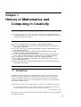
The most well-known case of these numbers is
32 + 42 = 52 .
Figure 1.1: The 3,4,5 triangle
A natural question to ask is whether there is a general pattern to such combinations
of a, b, c, and if we can be sure we have all such combinations. You can check that if
a2 + b2 = c2 , then if we multiply each number by a fixed other number, the resulting
numbers have the same property (e.g. 62 + 82 = 102 ). From the Babylonian texts,
they found a more interesting way of coming up with such numbers: if p, q are any
two positive numbers, then let
a = p2 − q2 ,
b = 2pq,
c = p2 + q2 .
Then a2 + b2 = c2 (this can be checked easily); it turns out that this gives all possible
numbers without a common factor, although that is a lot harder to show.
There are some characteristic features of mathematics here: there is an initial
discovery with useful practical consequences, which prompts more general
questions. Finding answers involves mathematical invention – it is a lot harder to
dream up the equations above than to check that they give us a good answer. In
fact, the work of Gödel and others shows—expressed informally—that we cannot
find all of mathematics just by deduction from what is already known, so a creative
leap is necessary for finding some new mathematical results.
1 http://www-history.mcs.st-andrews.ac.uk/Indexes/Babylonians.html
2
Arab Mathematics and Computation
1.3
Ancient Greece
Ancient Greece was important for the development of Western mathematical
thought; we owe the systematic development of geometry and the introduction of
the deductive method to the ancient Greeks (for deduction, see section 1.6), as well
as the discovery of irrational numbers.
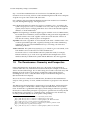
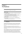
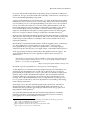
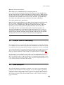
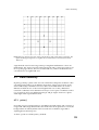
Let’s look at what we call Pythagoras’ Theorem 2 . Given any right-angled triangle
(the length of each of the sides does not have to be an integer), if we draw a square
of each side of the triangle, the sum of the areas of the two smaller squares is the
area of the largest square.
Figure 1.2: Pythagoras’s theorem
There are many different ways of showing this; you might try to think how this
could be proved in general. There are some animated versions of the proof3 , that
work by moving parts of the diagram around so that the different areas (and some
copies of them) can be put together in different ways. Remember that the claim is
that this relationship holds for all possible right-angled triangles. Coming up with a
way of showing that this is the case involves inventing new ways of thinking about
area and geometrical shape.
1.4
Arab Mathematics and Computation
In the period 800–1400, there was relatively little new mathematics being developed
in the West. However, in the Arab/Islamic part of the world, new ideas were
developed that affect the way we think about mathematics and represent it to this
2 http://www-history.mcs.st-andrews.ac.uk/Mathematicians/Pythagoras.html
3 http://www.mathsisfun.com/pythagoras.html
3
Creative Computing I: Image, Sound, Motion
day 4 . Not all the mathematicians involved were in fact Muslim (Jews and
Christians were involved), and it is worth remembering that North Africa and parts
of Spain were part of the Arab world at the time.
It is a tribute to this period that mathematical terms from Arabic have found their
way into the English language. Among these are:
zero The Roman numeral system does not have a number “zero”; nowadays, the
symbol “0” plays two roles, as a number on its own, and as a part of a numeral
system (in base 10, for example). Both these uses came to the West through the
influence of Arab mathematics 5 .
algebra The beginnings of modern algebra appear with the work of al-Khwarizmi6 ;
he treated rational numbers, irrational numbers and geometrical magnitudes as
algebraic entities. The word “algebra” itself comes from the title of his book
from the 9th century, “Hisab al-jabr w’al-muqabala”.
algorithm The term “algorithm” is in fact based on the name “al-Khwarizmi”. The
word has passed through Latin, originally referring to the Arabic numbering
system, but also associated with different ways of working out solutions to
arithmetic problems 7 .
Arabic numerals The symbols 0,1,2,3,4,5,6,7,8,9, to which we are accustomed, come
from Indian sources to the West via Arabic mathematics 8 .
It is much easier to work with this numeral system than with, for example,
Roman numerals; try to work out an algorithm for the multiplication of two
numbers directly in the Roman system and the difference becomes apparent.
1.5
The Renaissance: Geometry and Perspective
During the Renaissance in the West, there was a flowering of thought both in
sciences and in the arts, with interaction between them (for example, Leonardo da
Vinci’s anatomical drawings). It is worth looking at Leonardo’s Vitruvian man9 , and
thinking about how ideas on art, design, architecture and creativity interact,
including the use of two of the three basic shapes from Bauhaus design theory
(discussed in the next chapter).
We can look at one connection around this time, that between the mathematical
analysis of the geometry of vision, and the introduction of perspective into Western
art.
The Renaissance brought with it a questioning of received ideas, and an interest in
classical thought as a model that could be surpassed. Brunelleschi10 shows these
traits: he trained as a goldsmith and sculptor, while taking an interest in geometry.
In 1415, he worked out the principles of perspective: parallel lines in reality should
be depicted as converging to a “vanishing point”, and objects’ sizes should vary
inversely with their distance from the plane of the painting.
4 http://www-history.mcs.st-andrews.ac.uk/Indexes/Arabs.html
5 http://www-history.mcs.st-andrews.ac.uk/HistTopics/Zero.html
6 http://www-history.mcs.st-andrews.ac.uk/Biographies/Al-Khwarizmi.html
7 http://www.peak.org/
˜jeremy/calculators/alKwarizmi.html
8 http://www-history.mcs.st-andrews.ac.uk/HistTopics/Arabic_numerals.html
9 http://en.wikipedia.org/wiki/Vitruvian_Man
10 http://www-history.mcs.st-andrews.ac.uk/Biographies/Brunelleschi.html
4
Inventing Computational Thinking
At this time, earlier paintings depicted scenes “as they are”, such as in the work of
Simone Martini11 , rather than “as they are seen”.
The interest in the geometry of three-dimensional space can be seen in the work of
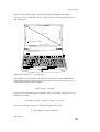
the artist Uccello12 . The artist Dürer is credited with the invention of “perspective
machines”, that helped artists master the new techniques, as seen in his own
etching, in Figure 1.3 below, of 1525. We might think that these devices would lead
to “mechanical” drawings, but in fact Dürer’s own work is anything but
mechanical; the mathematics of space had opened up new artistic possibilities.
Material available only to students registered on this module.
1.6
Inventing Computational Thinking
Computational devices and algorithmic ideas went hand in hand with mathematics
from the earliest times; think of the abacus13 , found throughout the world at
different times. Astronomy gave ways of predicting the seasons, and methods and
tools are associated with it, such as the astrolabe14 .
Leibniz15 was a German philosopher and mathematician, who lived from 1646 to
1716. As a philosopher, he tried to provide accounts of knowledge, of truth, and of
the relation of perception to the external world.
He thought that mathematics gave access to especially clear and uncontroversial
conclusions via calculations. He built a calculating machine, which he showed to the
Royal Society in London in 1673 – so his interests in this topic were not just
theoretical.
Leibniz thought that reasoning in general could be dealt with via calculation, if we
could express statements in what he called the Characteristica Universalis (universal
mathematics). Then, given rules to calculate correct conclusions, reasoning could be
done in this new language. Once we wrote down our knowledge in this special
language, reasoning could be replaced by computation.
He wrote:
Telescopes and microscopes have not been so useful to the eye as this instrument would
be in adding to the capacity of thought. . . . If we had it, we should be able to reason in
metaphysics and morals in much the same way as in geometry and analysis.
(Leibniz, quoted in Russell (1900))
11 http://www.ibiblio.org/wm/paint/auth/martini
12 http://abstract-art.com/abstract_illusionism/ai_03_put_into_persp.html
13 http://en.wikipedia.org/wiki/Abacus
14 http://en.wikipedia.org/wiki/Astrolabe
15 http://www-history.mcs.st-andrews.ac.uk/Mathematicians/Leibniz.html
5
Creative Computing I: Image, Sound, Motion
and also
If controversies were to arise, there would be no more need of disputation between two
philosophers than between two accountants. For it would suffice to take their pencils in
their hand, to sit down to their slates, and say to each other (with a friend as witness, if
they liked): Let us calculate.
(Leibniz, quoted in Russell (1900), p.169)
This idea of having machines use logic for themselves eventually became an
impetus for work in Artificial Intelligence.
Since the 19th century, other machines have been built to carry out calculations:
mechanical devices in the 19th century, up to programmable electronic machines
starting around 194516 . Back in 1834, Charles Babbage in England conceived a
mechanical computer programmable via punched cards (already in use in Jacquard
looms as “programs” to control pattern elements in weaving, via a “card reader”).
The computer, which was first described in 1837 and more fully in 1843, was called
the Analytical Engine17 . The 1843 description was extensively annotated by Ada
Lovelace18 , who worked closely with Babbage. In her notes, Lovelace outlined an
algorithm intended to be processed by the Analytical Engine, and is therefore
regarded by many as the first computer programmer19 . The construction of the
Analytical Engine was never completed, although a partial trial model was
assembled in 187120 .
It is striking how much of the mathematical theory of computation had been put in
place before there were any computers in existence, as we understand the term
today. Already in 1936, mathematical characterisations had been worked out,
describing which functions (over the natural numbers) could be computed. It had
been shown that there are some such functions that simply cannot be computed,
regardless of which programming language is used and however much time and
space is used in the computation. Alan Turing21 was one of the pioneers here, along
with Alonzo Church and Emil Post.
It had been a long-standing philosophical question whether machines can show
intelligence, and Alan Turing was also instrumental in provoking work in Artificial
Intelligence22 . His description of reasoning machines breathed new life into Leibniz’s
outline proposal: Turing argued that computers could in principle be made to
process sensed data following reasoning patterns as humans do, and would then be
to all intents and purposes acting intelligently.
The present-day Loebner competition23 in Artificial Intelligence is based directly on
Turing’s work.
16 http://en.wikipedia.org/wiki/History_of_computing_hardware
17 http://en.wikipedia.org/wiki/Analytical_Engine
18 http://www-history.mcs.st-andrews.ac.uk/Mathematicians/Lovelace.html
19 http://en.wikipedia.org/wiki/Ada_Lovelace
20 http://www.sciencemuseum.org.uk/objects/computing_and_data_processing/1878-3.aspx
21 http://www-history.mcs.st-andrews.ac.uk/Mathematicians/Turing.html
22 http://en.wikipedia.org/wiki/Turing_test
23 http://www.loebner.net/Prizef/loebner-prize.html
6
Mathematics and Music
1.7
Mathematics and Music
There has been an interplay between music and mathematics throughout the
development of both subjects (Fauvel, Flood and Wilson (2006) cover the history
and current state of this interaction). Pythagoras, whom we met above, and his
school, investigated how to produce different musical notes (pitches), e.g. by hitting
glasses filled with water to different heights, or bells of different sizes (see the
illustrations here24 ). It has been argued that this was the basis of the Ancient Greeks’
interest in rational numbers: the most important intervals in music can be obtained
by taking a vibrating string, e.g. guitar, and then not allowing the string to vibrate at
points at 21 , 13 , 41 . . . of the length of the string, so producing musical harmonics25 .
It was from Pythagorean times that mathematics was considered to be composed of
the four related studies: astronomy, geometry, arithmetic and music. This persisted
into medieval times, where throughout European universities up to the 16th
century the final topics studied at university formed the quadrivium, consisting of
just these subjects.
As for visual art, there was a renewed interest in understanding music and the
mathematics of sound during the Renaissance and later; an example is in the work
of the French mathematician Marin Mersenne26 who in 1627 published a book on
the mathematics of harmony “L’harmonie universelle”. (Mersenne is known today
because his name is attached to the so-called “Mersenne primes”, prime numbers of
the form 2p − 1 where p is itself prime.)
Later, mathematical analyses were made of the sound waves corresponding to a
single note at a fixed frequency; different instruments and different voices give
different sound colours (timbres), and it turns out surprisingly that the sound
waves involved can be described by a combination of sine waves at frequencies
n, 2n, 3n, . . . where n is the frequency of the base note. This technique of harmonic
analysis is due to the French mathematician Fourier27 , and is central to current
digital sound production techniques.28
We can look at an important recent example of how mathematics enabled new
sound worlds to be opened up, in the music of the Greek composer Iannis Xenakis
(1922–2001). Many of his ideas are laid out in his book “Formalized Music” (1992).
Xenakis was influenced by Ancient Greek culture, and collaborated with Le
Corbusier as an architect in France. He saw architecture as being about articulating
structures in space, while music involves deploying structures in time, in both cases
involving calculation and reasoning. An example in his early piece “Metastasis”,
shown in Figure 1.4, involves a musical version of creating curves out of a number
of straight lines.
Here each line corresponds to an instrument playing a note whose pitch varies
uniformly in time (quickly if the line is steep); the effect is of a mass of changing
sound which has edges that move in this “curved” way through time.
He introduced many other new musical possibilities – “Pithopratka” treats the
24 http://www.philophony.com/sensprop/pythagor.html
25 http://en.wikipedia.org/wiki/Harmonic
26 http://www-history.mcs.st-andrews.ac.uk/Mathematicians/Mersenne.html
27 http://www-history.mcs.st-andrews.ac.uk/Mathematicians/Fourier.html
28 We
will discuss these topics in much more detail in Chapter 5 of Volume 2 of this subject guide.
7
Creative Computing I: Image, Sound, Motion
Material available only to students registered on this module.
Figure 1.4: Xenakis: sketch for Metastasis. From: Iannis Xenakis, Formalized Music: Thought and
Mathematics in Composition, Bloomington: Indiana University Press, 1971, pg. 3.
individual musicians like molecules in a gas, moving according to chance though
the sound world, but still having predictable global properties, by making use of
the statistical mathematics of gases.
Xenakis showed us one way in which mathematical and computational ideas can be
liberating for the artist.
1.8
Some notes on additional reading
A good general overview of the history of mathematics is Steiner’s “Grammars of
Creation”(2001), though it supposes a good mathematical background. An account
that focuses more on the personalities is Bell’s “Men of Mathematics”(1986). An
excellent on-line resource for the history of mathematics is the The MacTutor
History of Mathematics archive29 .
We get a different feel for the invention of mathematics by looking at the way
mathematicians describe their own work. There is a collection of snippets from
mathematics through the ages in Fauvel and Gray’s “The History of Mathematics: a
Reader” (1987). Poincaré was a famous French mathematician who wrote about
mathematical invention; there is an interesting comparison between Poincaré and
29 http://www-history.mcs.st-andrews.ac.uk/index.html
8
Exercises
his contemporary the artist Marcel Duchamp by Gerald Holton30 . Hofstadter’s
“Gödel, Escher, Bach” (1999) remains the best popular account of the interplay
between mathematics, science and the arts, all seen as creative domains in their
different ways.
1.9
Summary and learning outcomes
This chapter set the scene for starting to learn about creative computing. It
presented some elements from the history of mathematics in a creative context, and
described how mathematicians and philosophers through the ages have made
conceptual leaps in mathematics by applying creativity and imagination. It also
introduced the work of some contemporary artists, and demonstrated how
mathematics has been influential in their work.
You should now be able to:
describe some of the major advances in the development of mathematics
look at different numeral systems and identify the significant differences
between them
discuss how creativity has influenced the advance of mathematical theory
identify the use of mathematical concepts in the work of some contemporary
artists
listen to music, look at architecture, examine a painting, and so forth, with a
perspective that includes the computational aspects of such artworks.
1.10
Exercises
1. Here are some parts of modern mathematical notation. Find out who first
introduced these symbols, and arrange them by the date they were first used.
(a) The number e, the base of natural logarithms: e = 2.72 . . . .
Z 1
R
(b) The integral sign , as in
x2 dx = 1/3.
(c) The square root sign
√
.
(d) The square root of -1, i =
0
√
−1.
(e) The symbol for infinity: ∞.
(f) The notation for complex numbers in the form z = x + iy, where x and y are
the real and imaginary parts of the number z.
2. Sketch out an algorithm for the addition of numbers given using Roman
numerals31 . The algorithm you sketch out should work for input numbers up to
MM (which is 2000 in the decimal system).
This way of representing numbers makes it harder to work out basic arithmetic
operations than the modern notation. Describe why it is the case that arithmetic
operations are harder to carry out in the Roman numeral system, compared
with the decimal system.
30 http://muse.jhu.edu/journals/leonardo/v034/34.2holton.html
31 http://www.romannumerals.co.uk/roman-numerals/numerals-chart.html
9
Creative Computing I: Image, Sound, Motion
3. One of the principles of perspective is that parallel straight lines in real life
should be depicted as converging to a “vanishing point”. This description
relates to the point of view of the viewer. Describe in more detail what a
vanishing point is, and how this relates to perspective.
Now explain why parallel lines should be shown in this way, by considering a
camera taking a photograph of a railway line, looking along the track, and
thinking about the angles involved when light travels in a straight line from the
track to the camera. In which cases would a vanishing point not be appropriate?
4. Alan Turing described what is now called the Turing Test; he suggested that the
question “can machines think?” is too vague to be useful, and could usefully be
replaced with the question “can machines pass the Turing Test?”.
Describe the Turing Test. Do you think this is a good test for whether or not a
machine can think? (This is a hotly disputed subject, with no agreed answer;
what is being asked for here is your own argument, with substantiation, for the
viewpoint you are taking.)
5. The composer John Cage often included a mathematical component to his
work, and the choreographer Merce Cunningham shared this interest. Look for
descriptions of their work together, and discuss how their approaches interact
with the topic of creative computing.
6. (a) It is interesting to compare Xenakis’s sketch for Metastasis with
architectural work he was doing at the same time with Le Corbusier for the
Philips Pavilion in the World Fair in Brussels in 1958. Find some images of
this building and Xenakis’s sketches for that.
(b) There are recordings of Xenakis’s Metastasis on the web. If you are
interested, find and listen to this seven-minute piece. The sketch shown in
Figure 1.4 above appears about 50 seconds before the end of this piece, and
is immediately followed by two bars of silence. In the sketch, time is
notated left to right, with pitch marked vertically. So initially we hear a set
of low-pitched sounds which get higher and closer together, and then after
roughly a second, a cluster of higher-pitched sounds enter. The sketch
covers about 7 seconds of music.
10
Chapter 2
The Bauhaus
Essential reading
http://www.bauhaus.de (site available in German and English)
Additional reading
Bayer, H., W. Gropius and I. Gropius (eds) Bauhaus 1919-1928 (Museum of Modern Art,
1976) [ISBN 0810960133].
Borchardt-Hume, A. (ed) Albers and Moholy-Nagy: from the Bauhaus to the New World (Tate
Publishing, 2006) [ISBN 1854376918 (hbk), 1854376381 (pbk)].
Eskilson, S. J. Graphic Design: A New History (Yale University Press, 2007) [ISBN
0300120117]. Chapter 6–The Bauhaus and the New Typography.
Itten, J. Design and Form, The Basic Course at the Bauhaus (Thames and Hudson, 1975)
[ISBN 0471289302].
Kandinsky, W. Point and Line to Plane (Dover, 1980) [ISBN 0486238083].
Naylor, G. The Bauhaus Reassessed (The Herbert Press, 1985) [ISBN 0906969298,
0906969301(pbk)].
Poling, C. V. Kandinsky’s Teaching at the Bauhaus; Colour Theory and Analytical Drawing
(Rizzoli, illustrated edition, 1986) [ISBN 0847807800].
2.1
Background
The importance of the Bauhaus in this course includes its attempts to rationalise
design and production. The formalisation of these creative ideas lends itself to
implementation in computer-aided design and visualisation tools. To understand
this we need to review the work of some important individuals and their
interactions.
The Bauhaus was founded by the architect Walter Gropius in Weimar in 1919. This
school of architecture and design in a small town in Germany was to have a
profound effect on artists, designers and art education in both Europe and the USA,
leading to long-term influences on society in terms of architecture, interior design
and furnishing.
Germany had undergone an industrial revolution following its unification from a
number of independent states in 1871. The speed with which Germany had shifted
from an agricultural country to an industrial one caused social problems. The
population of Germany greatly expanded over the 19th century. Large cities
developed where small villages had been and the small cheap dwellings built for
the workers led to slum conditions. Transportation infrastructure was expanded,
including new railways and roads. Daimler and Benz built their first motor cars in
11
Creative Computing I: Image, Sound, Motion
the 1880s. Major industries such as Krupps expanded from a small steel works in
Essen, to an enormous industrial complex manufacturing armaments.
Germany was now an important trading nation and with this rise in importance,
there was a related development in German art. Dresden and Munich, followed by
Berlin, emerged as artistic centres. The artists in the German Expressionist
movement were influenced by the work of Van Gogh and Gauguin with their use of
colour to express emotion. Based in Dresden the ‘Brücke’ artists—Kirchner, Heckel,
Bleyl and Schmidt-Rottluff—were influenced also by the linear quality of Gothic art
and the fact that the artist carvers were anonymous members of a guild which did
not differentiate between art and craft. The Brücke artists wanted their art to “speak
to the people”. They published a manifesto calling upon youth to revolt against old
established ideas.
In Munich a New Artists’ Association was formed. Members included Kandinsky,
Jawlinsky, Münter and Franz Marc. They organised an exhibition of work by
Picasso, Derain and Vlaminck in 1910, but the group broke up and Kandinsky and
Marc formed the ‘Blaue Reiter’ group. In a publication they produced, Kandinsky
wrote that distinctions between different art forms should be broken down.
Kandinsky had arrived in Germany from Russia in 1896. He had studied law, but
turned to art and art theories, writing “Concerning the Spiritual in Art”, a
justification for abstract art. Kandinsky had a deep interest in the relationship
between sound and colour (there is debate over whether he had the condition of
synesthesia), and this has an effect on the development of his art1 . He had an
interest in colour for its own sake, and over his career he moved away from the
representation of recognisable subjects and objects. By 1910 he had produced his
first abstract painting of basic shapes, lines and forms. In his “Compositions”,
Kandinsky carefully arranged shapes and colour to attempt to communicate
feelings to the spectator, whilst in his “Improvisations”, which were more freely
painted, he wished to express experiences and feelings.
New ideas concerning the direction of art were developing in other countries. In
Russia, Tatlin pioneered constructivism, an abstract art form that made use of
machinery and modern materials. In Holland, a group of artists published a journal
called De Stijl. Mondrian was the most famous member of the group. The austere,
abstract style had more influence on architecture than painting and also an
influence on designers working in the Bauhaus.
Walter Gropius (1863–1969) had been a student at the Weimar School of Arts and
Crafts when the Belgian architect Henri van de Velde had been its director. Van de
Velde pioneered the Art Nouveau style. He designed a building for the school
which was opened in 1907, offering courses in printing, weaving, ceramics, book
binding and precious metalwork. With growing xenophobia in Germany, van de
Velde left his position in 1915, and the school closed in the same year.
Before the outbreak of the 1914–1918 war, Gropius had worked in the design office
of Behrens at AEG where he had developed ideas for standardising components for
construction and written, with Behrens, a Memorandum on the Industrial
Prefabrication of Houses on a Unified Artistic Basis.
1 http://en.wikipedia.org/wiki/Synesthesia_in_art
12
Bauhaus developments with new staff
2.2
The Beginning of the Bauhaus
In 1907 an organisation called Werkbund, led by Muthesius, an architect, was
formed. Muthesius maintained that industry, not the artist, had the energy to make
cultural changes. He held that architecture should move towards standardisation.
Gropius disagreed with this theory, as he considered that the artist or architect
should determine the forms of buildings.
Gropius and his partner Adolf Mayer were successful architects before the First
World War. Gropius had designed the model factory for the Cologne exhibition, the
Fagus factory2,3 , furniture and a locomotive. After the war Gropius was asked by
the Weimar State Council to formulate his plans for establishing a school of art and
architecture. In 1919 Gropius was appointed as director.
2.2.1 Principles for the Bauhaus
Gropius produced the Bauhaus Manifesto to set out his aims for the school.
He wrote that all creative arts were to return to the crafts and there was to be no
difference between the artist and craftsman. Architecture was the supreme art form.
Artists must be trained to work for industry. Artists, architects, sculptors and
craftsmen should all work to one common goal.
The Bauhaus staff would consist of a master and a journeyman to each workshop,
ensuring that techniques as well as design ideas were brought together.
There were to be six categories of craft training:
Sculpture stonemasons, woodcarvers, ceramic workers and plaster casters
Metalwork blacksmiths, locksmiths, founders and metal turners
Cabinet making
Painting and decorating glass-painters, mosaic workers and enamellers
Printing etching, wood-engravers, lithographers and art printers
Weaving
Apart from studies in these areas, students would experience instruction in
drawing and painting, including colour theory, the science of materials and basic
business studies.
2.3
Bauhaus developments with new staff
Johannes Itten joined the Bauhaus in 1919. He developed the Basic Course of one
term’s length. Here the students were taught to develop self-confidence. They were
taught theories of form with emphasis on the simple basic forms of circle, triangle
and square. Compositions were made employing the three shapes. These shapes
2 http://www.greatbuildings.com/buildings/Fagus_Works.html
3 http://www.brynmawr.edu/Acads/Cities/wld/06790/06790m.html
13
Creative Computing I: Image, Sound, Motion
were derived from Cubism and were seen as historically primary in art. Also they
are independent of nature and easily produced, appearing in Itten’s Wood and
Metal Workshops. In addition, students learned colour theory in order to
understand the expressive qualities of colour and colour contrasts, and
consideration of materials and texture. The latter were considered essential for
commercial artists and industrial designers.
The Processing package, introduced later in this course, can be thought of as a
simple workbench providing a basic stock of elementary shapes and colours,
together with the tools to combine and manipulate these basic elements, to design
and produce novel products. Correspondingly, Bauhaus staff initiated what are
now some standard image manipulation techniques. For example, Itten (1975, p.21)
has an interesting ‘Light-dark analysis of a picture by Goya’, where the breakdown
is into a regular array of squares that predates modern ‘image pixelation’ by more
than half a century. Another example is ‘Happy Island’, which is an oil work on
canvas4 . The same Itten text has examples of image kaleidoscoping (1975, pp.56, 57)
using regular photographic darkroom techniques, but which can now be simply
carried out in standard image processing packages.
The Metal Workshop was founded to develop prototypes for mass production.
Gropius maintained that standardisation of goods was the means by which the
masses could acquire items, so designs should be suitable for furnishing a house.
The workshop was initially led by Itten, then, from 1923, by László Moholy-Nagy.
Marianne Brandt and William Wagensfeld achieved the most successful work.
Wagenfeld designed table lamps with straight shafts and an opaque glass shade5 .
Brandt produced metal ashtrays, lamps and other household objects. Her lamp
reflectors were made of nickel-plated metal, and had moveable shades and arms for
good light dispersion6,7 .
Brandt, who succeeded Moholy-Nagy as director of the Metal Workshop in 1928,
was the only woman on the permanent staff. Most women students joined the
Weaving Workshop where they experimented with techniques. They created
tapestries using a variety of materials and by 1931 made a range of handmade
fabrics in muted colours ideal for mass production8 .
Paul Klee and Wassily Kandinsky joined the Bauhaus in the early 1920s. Klee and
Kandinsky had both been members of Der Blaue Reiter. Klee developed an
independent theory of colour and an analysis of the creative process. His work was
derived from nature/landscapes, plants, sea, stars and buildings. Kandinsky
continued to work on his theories concerning the “science of art”, the underlying
elements and themes in discussing a theoretic approach to analysis and synthesis of
painting (see, for example, “Point and Line to Plane”, (Kandinsky, 1979)). Another
good source for examples of shape and colour work is “Kandinsky’s Teaching at the
Bauhaus” (Poling, 1982). There were debates within the Bauhaus concerning the
relevance of these ideas in an institution that placed technology at the heart of
experimentation and an analysis of material. However the painters stayed as their
fame contributed to the success of the school.
Sommerfeld House was designed by Gropius and Mayer in 1921 for a timber
merchant. Three students worked on the interior designs: Joost Schmidt made relief
4 http://metropolis.co.jp/tokyo/515/art.asp
5 http://www.bauhaus.de/english/bauhaus1919/werkstaetten/werkstaetten_metall.htm
6 http://www.architonic.com/mus/8100111/1
7 http://www.trocadero.com/MuseXX/items/142321/item142321store.html
8 http://www.bauhaus.de/english/bauhaus1919/werkstaetten/werkstaetten_weberei.htm
14
Movement towards Constructivism
carvings on the staircase, Josef Albers designed the stained glass windows and
Marcel Breuer designed the furniture. Breuer’s furniture was influenced by
Reitveld’s Red/Blue chair designed in 1917 and illustrated in De Stijl magazine9 .
2.4
Movement towards Constructivism
In 1923 László Moholy-Nagy was invited to teach at the Bauhaus to replace Itten.
He was a Constructivist whose work emphasised the importance of the machine.
Constructivism, he declared, could expand from an art form into industrial design.
Josef Albers had trained as an art teacher before becoming a Bauhaus student. He
now began working with Moholy-Nagy on teaching the Preliminary Course where,
without using workshop equipment, tasks were given to explore the nature of
materials. Moholy-Nagy directed experiments in form. He emphasised that, in an
industrial culture, the need to understand the load-bearing properties and other
characteristics of materials was essential, linking design and engineering.
Moholy-Nagy was interested in the development of photography and reflected
light compositions. He experimented with optical and acoustic equipment to make
new creations. A starting point in reading about their influence is
Borchardt-Hume’s edited collection “Albers and Mohol-Nagy: from the Bauhaus to
the New World” (2006).
In 1923, a Bauhaus student, Ludwig Hirschfeld-Mach, wrote a score for a colour
sonata of three bars using a combination of light and music. Lights and templates
were moved in time to the fugue-like music. In 1924 Hirschfeld-Mach wrote:
Yellow, red, green, blue in glowing intensity move about on the dark background of a
transparent linen screen—up, down, sideways. They join and overlappings and colour
blendings result.
(Bayer, Gropius and Gropius (1976), p.65)
Moholy-Nagy experimented with photography, producing photograms and
photomontages. He maintained that traditional painting was finished. The move
from working on a canvas to creating art through mechanical means meant that
artists were no longer involved with producing a piece of art. In 1922 Moholy-Nagy
ordered his ‘telephone abstract enamels’ from a factory. He described these works
as “enamel pictures executed by industrial methods”10 .
Moholy-Nagy was also involved with typography and page layout, which was
itself an art form. He moved away from static lay-outs to dynamic ones, especially
in poster work in the style of Lisitsky, a Russian Constructivist whose poster of 1919
shows a red, triangular wedge (representing the Communists) being driven into a
circle of white (the White Russian Army)11,12 . These symbols could be easily
understood even by an uneducated peasant population.
In 1923, while Germany was in the grip of rising inflation, a competition was held in
the Bauhaus to design an experimental house to demonstrate the abilities within the
school, the design to be chosen democratically by staff and students. Georg Muche,
who had joined the staff as a painter, won with a design for a single storey house,
9 http://www.terraingallery.org/Anthony-Romeo-Chair.html
10 http://www.mutualart.com/OpenArticle/Mind-the-Design/CA53B9419178DC4A
11 http://www.sovr.ru/english/show/virtual1.shtml
12 http://www.allposters.com/-st/Lazar-Lisitsky-Posters_c81955_.htm
15
Creative Computing I: Image, Sound, Motion
named “Haus am Horn”13 . Constructed from concrete, the main part of the house
was the living room lit by a clear-storey. Other, smaller rooms were set around it
including a small, easy-clean kitchen with built-in storage and where everything
was within reach. The aim was for economy of space, time and energy. The house
was furnished by members of the school.
The Bauhaus mounted an exhibition in 1923. There were lectures by Gropius and
Kandinsky and performances of the Triadic Ballet by Schlemmer14 who had painted
murals on the walls of the Bauhaus. Music was provided by the Bauhaus jazz band
as well as concerts at which works by Hindemith, Busoni and Stravinsky were
played. This made Weimar the focus of the avant-garde, but locally Hitler’s
National Socialists were gaining popularity and they cut the grant to the Bauhaus,
forcing it to re-locate to Dessau in April 1925.
Dessau was then an industrial town where Junkers had their aircraft factory. The
Bauhaus was amalgamated with the local trade school. Here the course was
re-assessed. Moholy-Nagy and Albers ran the preliminary course and
Moholy-Nagy also headed the Metal Workshop.
Marcel Breuer headed the Furniture Workshop while two other Bauhaus trained
designers, Herbert Bayer and Joost Schmidt, took on the Printing and Sculpture
Workshops. Georg Muche was given responsibility for the Weaving Workshop.
The school’s aim was to research the needs of modern households and produce
relevant designs that industry could produce in mass.
Gropius wrote:
The creation of standard types for all practical commodities of everyday use is a social
necessity.
(Gropius (1926)15 )
Muche designed a metal house in 1925 while the architects in Gropius’s office
designed a new Bauhaus building16,17 consisting of two L-shaped buildings with
flat roofs, one to house the students and the other to house the workshops. The
workshop had a curtain wall made of glass, that allowed people outside to see what
the students were creating.
Also built at this time were houses for the staff. They were made of concrete with
flat roofs, large windows and balconies. Each house had a studio. They were set in
landscaped gardens which were ten minutes walk from the Bauhaus18,19 .
In Dessau, the architects undertook a housing project for workers called the Torten
Estate20 . These were state financed and built at low cost. They were small
two-storey buildings made of concrete with flat roofs. Three hundred and sixteen
one-family units were built, each having three bedrooms, a kitchen-diner and a
living room. Central heating, double glazing and built-in cupboards were provided.
Each house had a large garden for growing vegetables. These houses were
intentionally experimental. Gropius decided that a national plan for housing was
13 http://www.hausamhorn.de/
14 http://www.meisterhaeuser.de/en/bewohner_5_schlemmer.html
15 http://www.mariabuszek.com/kcai/ConstrBau/Readings/GropPrdctn.pdf
16 http://www.bauhaus.de/english/bauhaus1919/architektur/index.htm
17 http://www.tu-harburg.de/b/kuehn/wg21.html
18 http://www.c20society.org.uk/docs/building/bauhaus.html
19 http://www.tu-harburg.de/b/kuehn/wg21.html
20 http://www.creen.demon.co.uk/travel/dessau.html
16
Movement towards Constructivism
necessary and should include financial planning, study of methods for industrial
production, storage of pre-fabricated units and study of efficient use of materials, as
well as standardising building components.
Gropius left the Bauhaus in 1927 and his place was taken by Hannes Meyer (Hans
Emil Meyer), whose interest was in social housing. Meyer advocated “a technical,
not an aesthetic process” to designing buildings. Past styles were to be rejected in
favour of modern. He laid stress on collective rather than individual work. He
believed that the new house should be pre-fabricated for building on site. Those
involved in building schemes should be economists, statisticians, industrial
engineers, standardisation designers, heating engineers and even climatologists,
before involving an architect. For Meyer architecture should be functional21 .
Moholy-Nagy insisted that designers should see their ideas through to completion
and take note of their impact on individuals and society. He foresaw the time when
electrically powered machines would reduce labour hours and the labour force
required by industry.
Marcel Breuer experimented with furniture made from tubular steel, for domestic
use. He welded pieces of steel together to make a chair22 . Moholy-Nagy
photographed the prototype. When it was published in a newspaper, people
wanted to buy the chair because it was light, simple, comfortable and inexpensive.
In the Typography Workshop, Herbert Bayer designed the Universal Type23 . He
argued strongly that the use of two alphabets (capitals and lowercase) was
unnecessary:
why should we write and print with two alphabets? both a large and a small sign are
not necessary to indicate a single sound. A = a. we do not speak a capital ’A’ and a
small ’a’. we need only a single alphabet.
(Bayer (1938) quoted from Eskilson (2007) p.276)
He aimed to produce guidelines for a more precise visual language.
As the depression worsened in Germany, designers began to feel that Meyer was
planning to turn the Bauhaus into a trade school. Before the move to Dessau,
painters had developed theories of space, form and colour that they taught to the
students. Meyer tried to diminish their influence. He increased the staff with
architects and began a programme on research into the requirements of social
housing. He re-organised the Bauhaus into four departments. Workshops were
now to operate for three days. The new departments were building, advertising,
interior design and textiles.
Workshops were to become self-financing through commissions. The interior
design department, under former student Alfred Arndt, designed low cost
furniture for mass production and wallpaper which became very popular and
helped finance the department24 .
The textile department liased with the manufacturing industries and Walter
Peterhans joined the advertising department where he focused on teaching
photography not as an art form but as a science25 .
21 http://www.bauhaus.de/english/bauhaus1919/architektur/architektur_meyer.htm
22 http://www.designmuseum.org/design/marcel-breuer
23 http://www.type.nu/bayer/univer.html
24 http://bauhaus-online.de/en/atlas/personen/alfred-arndt
25 http://www.ifa.de/a/a1/foto/ea1bpebi.htm
17
Creative Computing I: Image, Sound, Motion
Meyer was forced to leave the Bauhaus in 1930 by the Nazis, who accused him of
allowing a communist cell into the school.
Mies van der Rohr succeeded Meyer. He had worked with Gropius in Behrens’
office. He had begun to design skyscrapers and was a supporter of functionalism.
The school closed for a period and when it reopened it was more a school of
architecture than design.
2.5
The last phase of the Bauhaus in Germany
The Nazis had little sympathy with van der Rohr’s ideas on simplicity and
functionalism. The school in Dessau was closed and van der Rohr moved the
Bauhaus to Berlin. However, after a number of raids by the Nazis the school closed
down. Many of those who had worked there eventually settled in the United States
of America.
2.6
Summary and learning outcomes
This chapter has given an introduction to the Bauhaus in terms of its development,
its main participants, and its influence on the rationalisation of design,
manufacturing and production.
With a knowledge of the contents of this chapter and its associated reading you
should now be able to:
name the main person who drove the formation of the Bauhaus, state his
profession early in life, name the main area in which he developed ideas at
Behrens, and explain how this background shaped his statement of aims for the
Bauhaus
name the main contributors to the development of the Bauhaus and its courses,
and briefly describe the background and interests of each of those contributors
illustrate the practical orientation of the Bauhaus by listing the six categories of
craft training, and briefly state what was involved in each
list the three simple forms utilised in the Basic Course, state their derivation,
and give examples of artefacts, designed at the Bauhaus, that utilise those forms
name two of the fine artists involved in the Bauhaus who contributed to the
theory of colour, and describe those contributions
state who at the Bauhaus was the driving force behind the idea of creating art
by mechanical means, and give examples of his work created in this way
describe and illustrate the influence of the Bauhaus on the design of housing
and household artefacts
describe and illustrate how the Bauhaus influenced trends in design and
practice for manufacturing.
2.7
Exercises
Use the reading for this chapter and other relevant texts when working on the
following exercises. In your writing, be sure to place any material from sources in
18
The structure of the rest of this guide
quotation marks and identify the source at the point of use, and provide a full
reference list at the end (this is to ensure you avoid plagiarism—see the Study
Support section of the VLE for further advice). Long quotations have no value in
showing understanding or earning marks. In any assessment it is your own
contribution in your own words that matters.
1. Discuss the importance of the contributions of Itten and Albers/Moholy-Nagy
in the development of the Foundation Course at the Bauhaus. Include
consideration of the contrast between the Nature and Machine approaches and
their effects on teaching and outcomes for the students.
2. Discuss which of the Itten and Albers/Moholy-Nagy approaches to design
teaching lends itself most easily to implementation and expression, with
computer-aided tools for pictorial expression, such as the Processing package
used in this course. Include an appraisal of the benefits, or otherwise, of
possible languages of basic shapes (such as that of triangle, circle, square), and
their differing emphases on two- and three-dimensional work.
3. Discuss whether or not the approach of Kandinsky offers greater opportunities,
or greater difficulties, for artistic expression with a computer-based drawing
package, than the approaches of Itten and Albers/Moholy-Nagy.
2.8
The structure of the rest of this guide
The preceeding two chapters have provided some historical and conceptual context,
to allow detailed examination of some of the concepts in the use of computer
technology in making creative artefacts.
In the next chapter, we will look at the software package Processing, and the
following chapters will examine various concepts in visual design, that are
illustrated using Processing. While you work through the material, you should bear
in mind that you are expected to become familiar with using Processing, to
understand the computational and conceptual issues discussed here and also to
consider all of the work in a creative context.
19
Creative Computing I: Image, Sound, Motion
20
Chapter 3
Introduction to Processing
Essential reading
Reas, C. and B. Fry Processing: A Programming Handbook for Visual Designers and Artists
(MIT Press, 2007) [ISBN 0262182629].
Additional reading
Moggridge, B. Designing Interactions (MIT Press, 2006) [ISBN 0262134748]. Chapter 1–The
Mouse and the Desktop, Chapter 2–My PC.
Packer, R. and K. Jordan (eds) Multimedia: From Wagner to Virtual Reality (W. W. Norton
and Company, expanded edition, 2003) [ISBN 0393323757]. Chapter 13–Alan Kay, User
Interface: A Personal View.
The year 1984 saw the beginning of a major change in the creative industries which
was heralded by the arrival of personal computers with graphical user interfaces
(GUIs). The Apple Macintosh was the first widely-available personal computer that
could display image, sound, speech, music, video and text. This caught the
attention of the design industry and very soon sophisticated audio-visual software
packages became the main tools of creative professionals. Among these were
Adobe’s Photoshop, for editing and creating images, and Digidesign’s Sound
Designer II for editing audio and music. The What-You-See-Is-What-You-Get
(WYSIWYG) interface paradigm offered direct manipulation of media objects
simply by pointing and clicking.
All media became part of the everyday desktop computing environment and, as a
result, computing became an everyday tool in the creative industries. As the
capabilities of computers grew, so did the ease with which media could be
manipulated. Multimedia computing became a reality in the late 1980s and early
1990s, followed rapidly by the internet and world wide web.
3.1
Processing
We will develop our creative tools in a programming language called Processing.
Processing is an open source programming language and environment for
programming images, animation and sound. It is widely used by students, artists,
designers, architects, researchers and hobbyists for learning, prototyping and
production.
The Processing open source project was initiated by Casey Reas (UCLA
Design/Media Arts Department) and Ben Fry (School of Design, Carnegie Mellon
University). It is an outgrowth of ideas started in the Aesthetics and Computation
21
Creative Computing I: Image, Sound, Motion
Group at the MIT Media Laboratory, and inspired by an earlier Java-based language
called Design By Numbers by John Maeda, who is a world-renowned graphic
designer, visual artist, computer scientist and Professor of Media Arts and Sciences
at the MIT Media Laboratory.
Introduced in 2005, Processing is based on Java, and provides all the functionality
that Java offers. It was created to teach fundamentals of computer programming
within a visual context and to serve as a software sketchbook and professional
production tool. However, it was designed to be far simpler to use than the
standard Java distribution. Processing has a user-friendly integrated development
environment (IDE) and it has many pre-defined methods for performing graphical
and multimedia design tasks with very little user-written code.
As open source software, Processing is an ongoing project and is developed by artists
and designers as an alternative to proprietary software tools in the same domain.
Do I need to know Java to use Processing?
It is not essential to know how to program in Java in order to use Processing. This
subject guide and the essential reading will give you an adequate knowledge of the
Processing programming language. However, as the Processing language is based
upon Java, knowledge of Java will undoubtedly help you. We assume that you are
taking the CO1109 Introduction to Java and Object-Oriented Programming course at the
same time as this course (or have previously studied Java). You should find that
these two courses complement and mutually reinforce each other.
Which version of Processing should I use?
At the start of each academic year, we designate the latest version of Processing as
our standard version for this course. Any coursework that you submit will be
tested on the standard version, so it is best if you use this version. To find out what
version is the current standard for the course, look at the CO1112 Creative Computing
I pages on the VLE.
Which version of Processing is used in this subject guide?
The current version of Processing at the time of writing this guide was 2.1. Any
specific descriptions in this guide refer to this version; if the standard version in
your academic year is newer, some of the details may be different. Any important
differences will be highlighted on the VLE.
3.2
Installing Processing
Learning activity
Method 1. From our VLE
You can download the course’s current standard version of Processing from the
VLE. From the home page at http://computing.elearning.london.ac.uk,
navigate to Courses →CO1112 Creative Computing I: Image, Sound and Motion.
From there, click on the relevant link to download the installation file.
22
Code examples
Method 2. From processing.org
Alternatively, you can download Processing directly from the
http://processing.org website. However, note that the version available there
may be newer than the standard version being used for the course. While you may
wish to try out the latest version, remember that any submitted coursework will be
tested against the standard version of Processing. Therefore, you should always
check your coursework against the standard version before submitting it.
Once the installation file is downloaded:
Move the Processing installation file to a folder that you want to install Processing
to. For example, on Windows you might try making a directory C://Program
Files/Processing. Double click on the file and extract the contents to the new
directory. See processing.org/tutorials/gettingstarted/ for further instructions.
You should now make a shortcut to allow you to easily run the program. For
example, on Windows this can be done by right-clicking on the processing.exe
executable file and selecting the “make shortcut” menu item. Select the resulting
“processing.exe shortcut” and move it to the desktop. Now you can just go to the
desktop and click the Processing icon and it will launch the application.
3.3
A Quick Tour of Processing
In Computer Science, a program is the list of instructions that is written by a human
for a computer to execute. In Processing this list of instructions is called a sketch. This
is to emphasize that this programming language is designed for creative computing.
To see what this means, click on the program shortcut that you made in the activity
above. Once Processing is running click on the File menu and select Examples to
bring up a window that lists a large number of example sketches; see Figure 3.1.
Try opening one of the examples, such as Basics→Form→ShapePrimitives, by
double clicking on it. When the sketch opens, click on the Run button (which looks
like a conventional video or audio Play button—an equilateral triangle with a point
to the right) at the top left of the window. There are many example sketches for you
to try; see the exercises at the end of this chapter.
3.4
Code examples
The following chapters present many examples of Processing code to demonstrate
particular topics and features of the language. You are encouraged to experiment
with these examples, by making changes to see how the output is affected, and by
using them as the starting point for developing more complex programs. Many of
the example programs can be downloaded from the CO1112 Creative Computing I
pages on the VLE.
23
Creative Computing I: Image, Sound, Motion
Figure 3.1: Opening the Examples folder in Processing.
3.5
Summary and learning outcomes
This chapter has been primarily about introducing you to Processing, and describing
how to download, install and use it.
You should now be able to:
explain what Processing is and who wrote it
download Processing, install and run it
open and run the example sketches that are bundled with Processing.
3.6
Exercises
Open each of the five sketches listed below, and run them by pressing the Run
button at the top of the Processing application.
Try to understand how they work by looking at the code for each sketch in the text
area. You should recognise some of the commands from Java, but you will also
notice that Processing simplifies standard Java syntax.
24
Exercises
Write a brief explanation (two to three sentences) of what each sketch does.
I) Basics→Form→ShapePrimitives
II) Basics→Structure→WidthHeight
III) Topics→Drawing→ContinuousLines
IV) Topics→Drawing→Pattern
V) Basics→Input→MousePress
25
Creative Computing I: Image, Sound, Motion
26
Chapter 4
Origins
Essential reading
Reas, C. and B. Fry Processing: A Programming Handbook for Visual Designers and Artists
(MIT Press, 2007) [ISBN 0262182629]. Structure 1: Code Elements, Shape 1:
Coordinates, Shape 1: Primitive shapes; Gray values, Development 1: Sketching
software.
Additional reading
Wong, W. Principles of Form and Design (Wiley, 1993) [ISBN 0471285528]. Chapters 1 and
2.
4.1
Introduction
This chapter introduces the foundations of two-dimensional drawing in Processing.
The chapter assumes that you have succesfully installed Processing, understand how
to launch the application, and are able to type in the editing box.
4.2
The Processing display window
Visual artists create on a canvas, composers create on staff paper; in Processing we
create on a display window. The display window is a flat rectangular surface with
hundreds of thousands of pixels (picture elements) that can be controlled
individually to produce light at different intensities. In Processing we type
commands into a text document called a sketch. After we make a Processing sketch
we can play it by pressing the Run button, as if it were a music player or a video
player, for example. Via sketches, we control the individual pixels on the display
window. So, the pixels are the raw material that we manipulate in a visual sketch.
Note that we may create sound instead of a visual image, but for now we will
concern ourselves only with the visual domain.
We must be careful to make a distinction between the display window in Processing
and the display device that is attached to your computer, be it a laptop, a tablet, a
monitor on your desktop or maybe a wide-screen high-definition plasma display.
We will call these physical displays.
In Processing, the display window is an interface to a window that is displayed
automatically, see Figure 4.1. This window is sent to the display device via the
operating system. In contrast to Java, where we must explicitly program every
27
Creative Computing I: Image, Sound, Motion
Figure 4.1: The Processing environment showing a sketch and its corresponding display
window.
graphical interface element ourselves, the Processing environment will create a
window for us automatically, but we must provide the details of the size of the
window that we want.
For brevity, throughout this guide we will sometimes refer to the Processing display
window as the screen. However, when we do this, do keep in mind the distinction
between this and the physical display, as described above.
Learning activity
In any programming language, it is interesting to see what happens when we
provide the system with no input whatsoever. Let’s start by seeing what Processing
does if we do nothing.
Make a new Processing sketch.
Save the blank sketch to your Processing folder.
Try pressing Run on your blank sketch.
What happens?
28
size()
Comments on the activity
We might expect nothing to happen, but something happens. A blank display
window is drawn to the screen. What size do you think this display is?
4.3
size()
To change the size of the display window we use a built-in Processing command
called size(). You should go to the Processing Help→Reference menu item. This
launches your web browser with the Processing help pages. It is often useful to look
at the complete form of the Help pages rather than the abridged form. That way
you can see all the built-in commands in Processing (see Figure 4.2). Note that to
find the Help page entry for any of the built-in commands or the language
elements, type the command that you are looking for into a sketch window,
highlight the text, right-click and select Find in Reference from the pop-up menu.
Figure 4.2: The built-in Help pages in Processing.
The parentheses () mean that this command is a method that takes arguments.
Arguments are simply values that we use to control the behaviour of a method. The
full name of the size() method is size(int width, int height). This tells us
that the size() method requires two arguments, both of which are integers, and
they control the width and height of the Processing display window.
29
Creative Computing I: Image, Sound, Motion
The width is simply the number of pixels horizontally across the window, and the
height is the number of pixels the window will display vertically. For example, the
following Processing sketch makes a display window that is 128 pixels wide and 512
pixels high:
size(128,512);
This sketch consists of a single line of code. Try running it. In Processing, like many
other computer languages, individual chunks of code must be terminated by
semi-colons. This makes it easy for the Processing program to identify where each
statement ends. Line breaks are allowed between parts of a single statement, but
statements must be terminated with a semicolon.
Here are some other sizes for you to try. How they appear on your physical display
device depends on the type of device you are using, especially its physical dimensions
and screen resolution.
Learning activity
Launch Processing.
Make a new folder for your sketches.
Make a series of sketches consisting of display windows of the following different
sizes:
size(512,128);
size(128,512);
size(1024,128);
size(1024,768);
size(8192, 8192);
size(-1, -1);
Did all of these commands produce useful results?
If not, do you understand why not?
Save these sketches to your file system using the File→Save menu item.
Re-load the sketches using the File→Open menu item.
Try modifying and re-saving some of your sketches.
Comments on the activity
Processing automatically makes a new folder for your sketch and creates a special
file called a Processing Development Environment (PDE) file and places it in that
folder. You only need to choose the name and the top-level directory where you
want to save the sketch; Processing does the rest.
It is good practice to organise your files into directory trees in some systematic way.
For example, you might make a directory called CC1, and inside it make a directory
called Chapter6, then save your sketches for that chapter within that folder. This
way, it is easier to remember where your sketches are when you want to refer back
to them at a later time.
30
background()
When developing code in Processing (or any other language), you should get into
the habit of saving copies of your work (“ backing up”) at regular intervals. The
simplest way to do this is to decide on a naming convention for your sketches—for
example, you might call the first version of your sketch mysketch-version1.pde,
the next mysketch-version2.pde, etc.1 That way, if you make changes in your code
that you later wish to remove (or, worse, if you accidentally delete your sketch!), you
can easily revert to the most recently saved backup version.
4.4
background()
We now start to explore how to draw in our sketch. Just like paper, or a canvas, we
start with a background colour that we specify using the background() method.
Learning activity
Try typing and running the following sketch:
size(512,512);
background(0);
What do you see? Now try the following sketch:
size(512,512);
background(100);
and finally try:
size(512,512);
background(255);
Type in the sketches above and run them. What is the meaning of the number in the
brackets in the background() statements?
Comments on the activity
The number in the brackets is the level of light intensity that is emitted from each
pixel in the display window. It can take on values between 0 and 255 where 0 is zero
light intensity (black) and 255 is maximum light intensity (white). Values in between
are various shades of grey that get progressively lighter as the number gets larger.
Processing’s display window is a model for the physical display that you are
viewing. So increasing the value of the number argument of the background()
method increases intensity of light on the physical display. You are controlling the
display using a simple, yet powerful, software interface.
1 There are more sophisticated ways of backing up your code, for example by using a Version Control
System such as Git (http://git-scm.com).
31
Creative Computing I: Image, Sound, Motion
4.5
Coordinates
4.5.1 Cartesian Coordinate System
A point is the smallest unit of drawing in Processing. Each position on the display
window is labeled by its coordinate pair, (x, y):
Example
size(512,512);
background(255);
stroke(0);
point(256,256);
In this example, we have made the window 512 × 512 pixels, set the background
colour to white and the stroke colour to black. Type in this example. Can you see
the pixel in the centre?
The single pixel is a little too small for our purposes because the pixels are very tiny,
see Section 4.9. Instead, let us increase the size of what we can see by changing the
thickness of the stroke:
Example
size(512,512);
background(255);
stroke(0);
strokeWeight(10);
point(256,256);
Type in this example, what do you see? From now on we shall use a large stroke to
make points visible enough for us to see them.
4.6
The Origin
The most important point in the Cartesian coordinate system is the origin. This is
the point at (0,0), that is zero in the x-dimension and zero in the y-dimension. In
Processing, where is the point (0,0)? We shall call the point (0,0) the origin, or O, for
short. Not to be confused with 0 (zero).
Once we know the position of the origin, we can draw in the plane using points and
lines. The origin in Processing is the point in the top left corner.
This placement of the origin at the top left of the screen, with x-values increasing
from left to right and y-values increasing down the screen, is common in computer
graphics and image processing applications such as Processing and the Java
two-dimensional graphics libraries. However, this is a different position for the
32
Plane Geometry
Figure 4.3: The origin in Processing is the point in the top left corner, that is point (0,0). The
grid is made by placing lines at a regular interval in both the horizontal and vertical
directions.
origin than the usual location in geometry, as taught in mathematics courses. In
mathematics, the origin is usually at the bottom left with y-values increasing as we
move up the page. That is, here we use left-hand axes, while in mathematics it is
conventional to use right-hand axes.
4.7
Plane Geometry
In plane geometry, a plane is the area onto which lines and points are drawn. This
can simply be thought of as an infinitely large sheet, where each position on the
sheet is indexed by a number from zero to the screen width minus one for the x
dimension and from zero to the screen height minus one for the y dimension.
Cartesian coordinates in two dimensions always occur as pairs of numbers such as
(x1, y1) and (x2, y2) for two different points p1 and p2. Figure 4.3 shows a plane
with origin at the top left-hand corner.
4.7.1 point()
Now that we have a background, we can add foreground content. The concepts of
foreground and background will become much more developed later. For now, the
background is an initially blank solid-coloured canvas and the foreground is
anything that is drawn upon it.
To draw a point we call the point() method:
33
Creative Computing I: Image, Sound, Motion
size(512,512);
background(0);
stroke(255);
strokeWeight(1);
point(256,256);
What do you see? Each point on the Processing screen corresponds to a pixel on
your computer’s monitor. A pixel is the smallest unit of change that is possible on
your computer’s screen. Now try the following:
size(512,512);
background(0);
stroke(255);
strokeWeight(1);
point(256,256);
point(256,257);
point(256,258);
point(256,259);
point(256,260);
What do you see? What are the dimensions of what you see? Remember,
dimensions are measurements of an object’s width and height. In this case the
dimensions are width=1 pixel, height=5 pixels.
Learning activity
Figure 4.4: PointSketch, a simple mouse-controlled point drawing sketch.
Type in the sketch shown in Figure 4.4.
Run the sketch. What do you think it does?
(Hint: try pressing the left mouse button while moving the mouse pointer over the
display window.)
What is the name of the method defined in this sketch?
34
Lines
We will discuss the use of methods in later chapters, but how is the method being
used by Processing?
Figure 4.5: Output of the PointSketch sketch.
Comments on the activity
draw() is a built-in method. You should look at the help pages for a description of
what it is and how it works. Processing calls the draw() method automatically in a
loop. This allows us to make interactive drawing applications such as the one
shown in this example.
4.8
Lines
In Processing, a line is defined by two points that are joined by filling in all the points
in between. The line() method allows us to define the two end-points of a straight
line:
size(512,512);
background(255);
stroke(0);
strokeWeight(10);
line(100,200,200,200);
It doesn’t matter in which order the two points are specified. We would get the
same results with:
size(512,512);
background(255);
stroke(0);
strokeWeight(10);
line(200,200,100,200);
These two describe the same line. We can check our intuition by looking just at the
end points alone:
size(512,512);
strokeWeight(10);
point(100,200);
point(200,200);
35
Creative Computing I: Image, Sound, Motion
size(512,512);
strokeWeight(10);
point(200,200);
point(100,200);
It is the same two points, so the same line will be drawn, the direction of drawing is
different, but that has no influence on what we see, the same pixels will get coloured
in both cases.
4.8.1 Zero-Based Indexing
The screen we’ve been using is 512 × 512 pixels. But, the pixels are addressed in the
range 0–511. This type of indexing is called zero-based indexing and it is the form
of addressing used in Java and in some other programming languages such as C
and C++. We must remember that the pixel indexed by the number 512 is actually
the 513th pixel; this is off the screen because the last visible pixel is 511. How can we
make a screen where pixel number 512, in either the x-dimension or y-dimension, is
included on the screen? The answer is that we make the screen at least 513 pixels in
its width dimension, x, and height dimension, y. For example:
size(513,513);
line(512,0,512,512);
Here, all the pixels at position 512 in x or 512 in y are drawn because the screen is
513 pixels wide and 513 pixels tall.
4.9
Size of a pixel
Pixels can be seen as the individual light sources that are packed together on your
computer’s display to make an image. They are the smallest unit of control that we
have in making an image. We start our creative computing journey by learning how
to manipulate pixels to draw images on the display device.
Before we embark on drawing to our display device, it will be useful to know how
big the pixels are and, therefore, how big the screen that we are drawing to is. In
short, we would like to know the dimensions of our display and of our created
images.
To work out these sizes, we need to know two things. The first is the size of the
physical display, and the second is the display resolution. The size of a pixel, then,
is its width and height in standard physical units.
Computer displays are measured by the length of the diagonal. For example, I am
currently writing this subject guide on a laptop computer that has a 15-inch screen,
however, let us work in centimeters for the purpose of international
standardisation. An inch is 2.54 centimeters (cm) so 15 inches is 15 × 2.54 = 38.1cm,
this is the distance from the top left to the bottom right of the screen, a diagonal line.
Figure 4.6 shows the monitor and the diagonal length of 38.1 cm. From the
specifications of my laptop given in its user manual, I know that its display has an
aspect ratio of 4/3; this is the ratio of the width to the height of the screen. This
means that the width is 4/3 or 33.33% larger than the height.
36
Size of a pixel
15in = 38.1cm
22.86cm = 768 pixels
Even if we are unable simply to measure the height and width of the display
directly, we can calculate these values as long as we know the (diagonal) screen size
and aspect ratio.
1 pixel = 0.029cm x 0.029cm
30.48cm = 1024 pixels
Figure 4.6: The dimensions of a laptop display.
By Pythagoras’ Theorem we know that the sum of the squares of the width and the
height equal the square of the diagonal length. We also know the aspect ratio, so we
can write down the following equation:
width2 + height2 = diagonal2
We know that width and height are related by width = aspectRatio × height. So we can
substitute for width:
(aspectRatio × height)2 + height2 = diagonal2 = (38.1cm)2
Now we rearrange the equation to obtain the height of the screen:
(1 + aspectRatio2 ) × height2 = (38.1cm)2
and finally:
37
Creative Computing I: Image, Sound, Motion
height =
q
(38.1cm)2 /(1 + (4/3)2 ) = 22.86cm
width = 4/3 × 22.86cm = 30.48cm
I know that my laptop display has a resolution of 1024 × 768 pixels. Now, we can
calculate the size of a pixel by dividing the width of the display by 1024, the total
number of pixels across the screen, or the height by 768, the total number of pixels
down the screen. We find that the width and height measurements of a pixel are
each 0.0298cm. That means there are 33.59 pixels active to make a line of pixels that
is a centimeter across and 33.592 ≈ 1129 pixels to fill a square centimeter (≈ means
approximately; the actual answer is 1128.678 pixels but we have rounded the
answer to the nearest whole number of pixels).
Learning activity
How many pixels are there in the whole screen assuming the 1024 × 768 resolution?
If stretched out in one long line, how long would this single-line display be?
Comments on the activity
To work out how many pixels there are in total we multiply the dimensions together.
For example, 1024 × 768 = 786432 pixels.
To work out how many centimeters a line of this many pixels would be, we calculate
786432 × 0.0298 = 23435.6 cm– that is ≈ 234 meters or 0.23 kilometers.
As an illustration of how to use Processing to work out the answers to the display
dimension problem, Figures 4.7 and 4.8 show a Processing sketch that computes
these dimensions, and its output. Don’t worry if you don’t understand all the
syntax for now, you will learn what it all means in your Java course and in later
sections of this subject guide. But see if you can find where the diagonal dimension
and aspect ratio are specified, and where the answers to the screen width and
height, and dimensions of a single pixel are calculated.
While we are looking at this sketch, it is worth highlighting one aspect that is often
a source of error for novice programmers. Notice that the variable A is defined as:
float A = 4.0/3.0; // correct
You might wonder why we did not just use:
float A = 4/3;
// incorrect!
The reason is that 4 and 3 are treated as integers by Processing and Java, and the
result of dividing two integers is also an integer. So in this case 4/3 would be
rounded down to the closest integer, giving a result of 1. This then gets assigned to
variable A, which is a float, so A takes the floating point value 1.0. In order to avoid
these integer arithemic problems when we desire an answer as a floating point
number, we specify the numbers to be divided as floats from the start. Hence,
4.0/3.0 in this example gives us the answer that we want, which is 1.33333.
38
Size of a pixel
// Solve the screen pixel size problem
float D = 38.1;
// Length
float A = 4.0/3.0;
// Aspect
float h = sqrt(pow(D,2)/(pow(A,2)+1)); // Height
float hPix = 768;
// Height
// Go backwards to check our result
float d = sqrt(pow(A*h,2)+pow(h,2));
// Now print the results
println("All Screen Units in Centimeters");
println("screen diagonal = " + d);
println("screen width
= " + A*h);
println("screen height
= " + h);
= " + h/hPix);
println("pixel width
println("pixel height
= " + h/hPix);
println("pixels per cm
= " + 1/(h/hPix));
= " + A*hPix*hPix);
println("total pixels
println("total pixel cms = " + A*hPix*h);
of diagonal
ratio
(cm)
(pixels)
Figure 4.7: screenMath, a Processing sketch that calculates the size of pixels for given screen
diagonal length D, aspect ratio A and vertical height in pixels hPix.
Figure 4.8: Text output of screenMath sketch.
Learning activity
Type in the Processing sketch of Figure 4.7. Look in your computer’s User Manual
to find the diagonal length and aspect ratio of your display device. Change these
values in the Processing sketch and run it.
a) How big is a pixel on your display device?
b) How many pixels per centimeter fit on your display device?
c) For a 38.1cm display, with resolution 1024 × 768 pixels, what is the size of a
512 × 512 Processing sketch in cm2 ?
Comments on the activity
Hint: The first two lines define the diagonal length and aspect ratio of the screen.
The fourth line defines the screen resolution in the y-dimension.
39
Creative Computing I: Image, Sound, Motion
Learning activity
Type in the following short Processing sketch:
void setup() {
println("display: " + displayWidth + "x" + displayHeight);
println("toolkit: " +
java.awt.Toolkit.getDefaultToolkit().getScreenResolution() + " dpi");
}
Run the sketch and look at the text output.
Comments on the activity
This sketch makes use of the Processing variables displayWidth and
displayHeight, which give the dimensions of the entire physical display (not just
the Processing display window).
The sketch also calls a library method in the underlying Java AWT toolkit to obtain
the Dots Per Inch (dpi) density of the physical display.
These methods can be useful when writing code for deployment on devices of
unknown display size.
4.10
Summary and learning outcomes
In this chapter, we have seen that we can turn the display of individual pixels on
and off using the point(x,y) method. Each pixel on the display window has a
unique two number address; just like we use latitude and longitude to identify
locations on the globe, we need an x-value and a y-value. These values are the
number of pixels to count in the x direction from left to right starting at 0, and the
number of pixels to count in the y-dimension starting from the top at 0 pixels. Just
as the combination of a particular latitude and longitude reading uniquely
identifies a specific place on the globe, both the x-value and y-value together
uniquely identify a pixel on the display window. The same pair of x-value and
y-value will always identify that same specific place on the Processing window.
It is possible to turn each individual display pixel on and off to make points on the
display window. A series of points in a row makes a line. But the points are very
small (how small?) so it takes a lot of points in a row to produce a line that is
significant.
To avoid the repetitive turning on and off of pixels to make lines, or other shapes,
we use the pre-defined line command as part of a Processing sketch. A sketch is
entered as statements separated by a semicolon. The semicolon is required for the
machine to be able to read and interpret the sketch, and a new line at the end of a
statement is optional and is for human readability of the sketch.
The line() method takes two pairs of numbers that represent the start point and
the end point of the line, and joins them by filling in the pixels in between. So, when
we draw lines in computing, we are really drawing a series of points. In this case
40
Exercises
we let an algorithm decide which points to fill in to draw the line, so there is already
computing going on under our noses. The algorithm for drawing lines is quite
complicated and is covered in a later section. For now, it suffices that lines are really
a collection of points with the property that the points join the end points by a
straight line, the shortest possible pattern of connected turned-on pixels between
two points on the display window.
We now have a method for joining two points with a line. In the next chapter, we
will see how lines can be made to have many different meanings.
You should now be able to:
describe what Cartesian coordinates are, and how the origin relates to these
explain what the Processing methods size() background(), point() and
line() do
describe what a pixel is and how this relates to the Processing display window
and to the physical display
write Processing sketches to draw pictures using points and simple lines.
4.11
Exercises
1. In section 4.2 you created a blank sketch, and were asked what size you thought
the sketch was. Without guessing or simply using judgement, how would you
find out the actual size? Why do you think this particular size is used as a
default? Note that when we talk about size, we could be referring to actual
lengths, or to numbers of pixels; it is important to become comfortable about
both of these uses.
2. In Processing, what is the difference between a sketch and a display window?
Why does Processing need both?
3. In Section 4.5.1 you saw an example where we used strokeWeight() to change
the thickness of the stroke. What is actually happening when this is done? What
is the relation between the pixels and the point? At the end of that section we
say that we will use a large stroke to make points more visible. Why then is it
useful for us to have pixels as small as they are? Would not making the physical
size of a pixel bigger improve visibility? What do we lose when we do this?
4. Write a Processing sketch that covers the display window with vertical lines.
Now modify it to do horizonal ones as well. Think about the distance between
the vertical lines, and the distance between the horizontal lines. You could
make them evenly spaced, or you could try to make them less regular. See what
kinds of pictures you can come up with just through innovative use of drawing
lines — this does not purely have to be through spacing; there are many other
creative dimensions that you can explore. Also, think about this in terms of the
previous chapters on the Bauhaus, and creativity in mathematics. In the next
chapter you will learn more about lines in Processing and lines as a creative
vehicle, but for now, try to see how much you can do with what you already
know.
5. Does a bigger physical display size mean there are more or less (or the same
number of) pixels on the screen? Dicuss this, and think about what it means for
Processing and its implementation — will Processing run in the same way on
computers with different sized screens and screen resolutions?
41
Creative Computing I: Image, Sound, Motion
42
Creative computing I:
image, sound and motion
Volume 2
M. Casey with T. Taylor and M. Magas
CO1112
2014
Undergraduate study in
Computing and related programmes
This is an extract from a subject guide for an undergraduate course offered as part of the
University of London International Programmes in Computing. Materials for these programmes
are developed by academics at Goldsmiths.
For more information, see: www.londoninternational.ac.uk
This subject guide was prepared for the University of London International Programmes by:
Michael Casey, Department of Music, Dartmouth College, USA
Tim Taylor, Department of Computing, Goldsmiths, University of London
Michela Magas, Goldsmiths Digital Studios, University of London
Additional help with production was provided by:
Sarah Rauchas, Department of Computing, Goldsmiths, University of London
This is one of a series of subject guides published by the University. We regret that due to pressure of
work the authors are unable to enter into any correspondence relating to, or arising from, the guide.
If you have any comments on this subject guide, favourable or unfavourable, please use the form at
the back of this guide.
First published 2008
This edition published 2014
University of London International Programmes
Publications Office
32 Russell Square
London WC1B 5DN
United Kingdom
www.londoninternational.ac.uk
Published by: University of London
© University of London 2014
The University of London asserts copyright over all material in this subject guide except where
otherwise indicated. All rights reserved. No part of this work may be reproduced in any form, or
by any means, without permission in writing from the publisher. We make every effort to respect
copyright. If you think we have inadvertently used your copyright material, please let us know.
Contents
Preface
1 Colour
1.1 Introduction . . . . . . . . . . . . . . . . .
1.2 Processing color type . . . . . . . . . . . .
1.3 RGB colour space . . . . . . . . . . . . . .
1.3.1 Defining color values . . . . . . .
1.3.2 Colour mixing . . . . . . . . . . . .
1.3.3 Colour gradients . . . . . . . . . .
1.3.4 Secondary colours . . . . . . . . .
1.3.5 Tertiary colours . . . . . . . . . . .
1.3.6 Transparency and colour blending
1.4 HSB colour space . . . . . . . . . . . . . .
1.5 Colour schemes . . . . . . . . . . . . . . .
1.5.1 Two-colour schemes . . . . . . . .
1.5.2 Three-colour schemes . . . . . . .
1.6 Summary . . . . . . . . . . . . . . . . . .
1.7 Exercises . . . . . . . . . . . . . . . . . . .
v
.
.
.
.
.
.
.
.
.
.
.
.
.
.
.
.
.
.
.
.
.
.
.
.
.
.
.
.
.
.
.
.
.
.
.
.
.
.
.
.
.
.
.
.
.
.
.
.
.
.
.
.
.
.
.
.
.
.
.
.
.
.
.
.
.
.
.
.
.
.
.
.
.
.
.
.
.
.
.
.
.
.
.
.
.
.
.
.
.
.
.
.
.
.
.
.
.
.
.
.
.
.
.
.
.
.
.
.
.
.
.
.
.
.
.
.
.
.
.
.
.
.
.
.
.
.
.
.
.
.
.
.
.
.
.
.
.
.
.
.
.
.
.
.
.
.
.
.
.
.
.
.
.
.
.
.
.
.
.
.
.
.
.
.
.
.
.
.
.
.
.
.
.
.
.
.
.
.
.
.
.
.
.
.
.
.
.
.
.
.
.
.
.
.
.
.
.
.
.
.
.
.
.
.
.
.
.
.
.
.
.
.
.
.
.
.
.
.
.
.
.
.
.
.
.
.
.
.
.
.
.
.
.
.
.
.
.
.
.
.
2 3D Graphics
2.1 Introduction . . . . . . . . . . . . . . . . . . . . . . . . . . . . . . . . .
2.2 3D coordinate system . . . . . . . . . . . . . . . . . . . . . . . . . . . .
2.2.1 The screen (viewport) . . . . . . . . . . . . . . . . . . . . . . .
2.2.2 3D rendering . . . . . . . . . . . . . . . . . . . . . . . . . . . .
2.2.3 3D lines . . . . . . . . . . . . . . . . . . . . . . . . . . . . . . .
2.2.4 Using OpenGL . . . . . . . . . . . . . . . . . . . . . . . . . . .
2.3 3D drawing . . . . . . . . . . . . . . . . . . . . . . . . . . . . . . . . .
2.3.1 3D primitives . . . . . . . . . . . . . . . . . . . . . . . . . . . .
2.3.2 beginShape(), endShape() . . . . . . . . . . . . . . . . . . . .
2.3.3 Perspective . . . . . . . . . . . . . . . . . . . . . . . . . . . . .
2.4 3D transformations . . . . . . . . . . . . . . . . . . . . . . . . . . . . .
2.4.1 translate(x,y,z) . . . . . . . . . . . . . . . . . . . . . . . . .
2.4.2 scale(sx,sy,sz) . . . . . . . . . . . . . . . . . . . . . . . . .
2.4.3 rotateZ(), rotateY(), rotateX() . . . . . . . . . . . . . . .
2.4.4 Camera transformations . . . . . . . . . . . . . . . . . . . . . .
2.4.5 pushMatrix(), popMatrix() . . . . . . . . . . . . . . . . . . .
2.4.6 Lights . . . . . . . . . . . . . . . . . . . . . . . . . . . . . . . .
2.5 Texture mapping . . . . . . . . . . . . . . . . . . . . . . . . . . . . . .
2.5.1 Transparent textures . . . . . . . . . . . . . . . . . . . . . . . .
2.6 Algebra for perspective and affine transformations; point and line . . .
2.6.1 Vectors and matrices; addition and multiplication . . . . . . . .
2.6.2 Translation, scaling and rotation of objects in 2-dimensional coordinate space . . . . . . . . . . . . . . . . . . . . . . . . . . .
2.6.3 Perspective . . . . . . . . . . . . . . . . . . . . . . . . . . . . .
2.6.4 Translation, scaling and rotation of objects in 3-dimensional coordinate space . . . . . . . . . . . . . . . . . . . . . . . . . . .
2.6.5 Point and line in two and three dimensions . . . . . . . . . . .
1
1
1
2
3
5
7
8
11
13
18
23
23
23
27
27
29
29
30
30
32
32
33
34
34
34
36
36
37
39
42
45
46
48
48
53
54
54
58
61
62
65
i
Creative Computing 1: Image, Sound, Motion
2.7 Summary . . . . . . . . . . . . . . . . . . . . . . . . . . . . . . . . . .
2.8 Exercises . . . . . . . . . . . . . . . . . . . . . . . . . . . . . . . . . . .
3 3D Motion and Control
3.1 Introduction . . . . . . . . . . . . .
3.2 Motion in a straight line . . . . . .
3.2.1 Camera motion . . . . . . .
3.2.2 Camera transformations . .
3.2.3 Motion parallax . . . . . . .
3.3 Circular motion . . . . . . . . . . .
3.4 Motion control . . . . . . . . . . .
3.4.1 Types of navigation . . . . .
3.4.2 Mouse . . . . . . . . . . . .
3.4.3 Mouse flythrough . . . . . .
3.4.4 Keyboard . . . . . . . . . .
3.5 Creative applications of 3D motion
3.5.1 A 3D paint brush . . . . . .
3.5.2 Painting by 3D swarms . . .
3.5.3 Painting by gestures . . . .
3.6 Summary . . . . . . . . . . . . . .
3.7 Exercises . . . . . . . . . . . . . . .
ii
.
.
.
.
.
.
.
.
.
.
.
.
.
.
.
.
.
.
.
.
.
.
.
.
.
.
.
.
.
.
.
.
.
.
.
.
.
.
.
.
.
.
.
.
.
.
.
.
.
.
.
.
.
.
.
.
.
.
.
.
.
.
.
.
.
.
.
.
.
.
.
.
.
.
.
.
.
.
.
.
.
.
.
.
.
.
.
.
.
.
.
.
.
.
.
.
.
.
.
.
.
.
.
.
.
.
.
.
.
.
.
.
.
.
.
.
.
.
.
.
.
.
.
.
.
.
.
.
.
.
.
.
.
.
.
.
.
.
.
.
.
.
.
.
.
.
.
.
.
.
.
.
.
.
.
.
.
.
.
.
.
.
.
.
.
.
.
.
.
.
.
.
.
.
.
.
.
.
.
.
.
.
.
.
.
.
.
.
.
.
.
.
.
.
.
.
.
.
.
.
.
.
.
.
.
.
.
.
.
.
.
.
.
.
.
.
.
.
.
.
.
.
.
.
.
.
.
.
.
.
.
.
.
.
.
.
.
.
.
.
.
.
.
.
.
.
.
.
.
.
.
.
.
.
.
.
.
.
.
.
.
.
.
.
.
.
.
.
.
.
.
.
.
.
.
.
.
.
.
.
.
.
.
.
.
.
.
.
.
4 Image
4.1 Introduction . . . . . . . . . . . . . . . . . . . .
4.2 PImage . . . . . . . . . . . . . . . . . . . . . . .
4.2.1 Image formats and encoding algorithms
4.2.2 PImage methods . . . . . . . . . . . . .
4.3 Image display . . . . . . . . . . . . . . . . . . .
4.3.1 Image crop . . . . . . . . . . . . . . . .
4.4 Image transformation . . . . . . . . . . . . . .
4.4.1 Image scaling . . . . . . . . . . . . . . .
4.4.2 Coordinate system transformations . . .
4.4.3 3D transformations . . . . . . . . . . . .
4.5 Layers . . . . . . . . . . . . . . . . . . . . . . .
4.6 Summary . . . . . . . . . . . . . . . . . . . . .
4.7 Exercises . . . . . . . . . . . . . . . . . . . . . .
.
.
.
.
.
.
.
.
.
.
.
.
.
.
.
.
.
.
.
.
.
.
.
.
.
.
.
.
.
.
.
.
.
.
.
.
.
.
.
.
.
.
.
.
.
.
.
.
.
.
.
.
.
.
.
.
.
.
.
.
.
.
.
.
.
.
.
.
.
.
.
.
.
.
.
.
.
.
.
.
.
.
.
.
.
.
.
.
.
.
.
.
.
.
.
.
.
.
.
.
.
.
.
.
.
.
.
.
.
.
.
.
.
.
.
.
.
.
.
.
.
.
.
.
.
.
.
.
.
.
.
.
.
.
.
.
.
.
.
.
.
.
.
.
.
.
.
.
.
.
.
.
.
.
.
.
89
. 89
. 89
. 90
. 90
. 91
. 92
. 92
. 92
. 95
. 97
. 98
. 104
. 104
5 Sound
5.1 Introduction . . . . . . . . . . . . . . . .
5.2 Digital audio . . . . . . . . . . . . . . .
5.2.1 Sampling . . . . . . . . . . . . .
5.2.2 Displaying a waveform . . . . . .
5.3 Audio file formats . . . . . . . . . . . . .
5.4 Audio in Processing . . . . . . . . . . . .
5.5 Installing the Sonia library in Processing
5.6 Playing a PCM sound file . . . . . . . . .
5.6.1 Adjusting the playback rate . . .
5.7 Digital audio synthesis . . . . . . . . . .
5.7.1 Sine wave . . . . . . . . . . . . .
5.7.2 The digital Theremin . . . . . . .
5.7.3 Square wave synthesis . . . . . .
5.7.4 Noise synthesis . . . . . . . . . .
5.8 Music synthesis . . . . . . . . . . . . . .
5.8.1 Rhythm . . . . . . . . . . . . . .
5.9 Summary . . . . . . . . . . . . . . . . .
.
.
.
.
.
.
.
.
.
.
.
.
.
.
.
.
.
.
.
.
.
.
.
.
.
.
.
.
.
.
.
.
.
.
.
.
.
.
.
.
.
.
.
.
.
.
.
.
.
.
.
.
.
.
.
.
.
.
.
.
.
.
.
.
.
.
.
.
.
.
.
.
.
.
.
.
.
.
.
.
.
.
.
.
.
.
.
.
.
.
.
.
.
.
.
.
.
.
.
.
.
.
.
.
.
.
.
.
.
.
.
.
.
.
.
.
.
.
.
.
.
.
.
.
.
.
.
.
.
.
.
.
.
.
.
.
.
.
.
.
.
.
.
.
.
.
.
.
.
.
.
.
.
.
.
.
.
.
.
.
.
.
.
.
.
.
.
.
.
.
.
.
.
.
.
.
.
.
.
.
.
.
.
.
.
.
.
.
.
.
.
.
.
.
.
.
.
.
.
.
.
.
.
.
.
.
.
.
.
.
.
.
.
.
.
.
.
.
.
.
.
.
.
.
.
.
.
.
.
.
.
.
.
.
.
.
.
.
.
.
.
.
.
.
.
.
.
.
.
.
.
.
.
.
.
69
69
69
70
72
72
74
75
75
75
76
78
79
79
83
83
83
87
.
.
.
.
.
.
.
.
.
.
.
.
.
.
.
.
.
.
.
.
.
.
.
.
.
.
.
.
.
.
.
.
.
.
.
.
.
.
.
.
.
.
.
.
.
.
.
.
.
.
.
66
67
.
.
.
.
.
.
.
.
.
.
.
.
.
.
.
.
.
.
.
.
.
.
.
.
.
.
.
.
.
.
.
.
.
.
105
105
105
106
111
112
112
113
114
114
115
115
120
122
122
125
125
127
5.10 Exercises . . . . . . . . . . . . . . . . . . . . . . . . . . . . . . . . . . . 127
6 Generative Systems
6.1 Introduction . . . . . . . . . . . . . . . . . . . . . . . . . . . .
6.2 Fractals . . . . . . . . . . . . . . . . . . . . . . . . . . . . . .
6.2.1 Iterated function systems and substitution systems . .
6.2.2 L-systems . . . . . . . . . . . . . . . . . . . . . . . . .
6.2.3 The Koch snowflake . . . . . . . . . . . . . . . . . . .
6.2.4 Two-handed substitutions . . . . . . . . . . . . . . . .
6.2.5 Plant modelling with bracketed L-systems . . . . . . .
6.3 Genetic algorithms . . . . . . . . . . . . . . . . . . . . . . . .
6.3.1 The Blind Watchmaker algorithm . . . . . . . . . . . .
6.3.2 User-guided genetic algorithms versus fitness functions
6.3.3 Biomorphs . . . . . . . . . . . . . . . . . . . . . . . .
6.3.4 Modelling genetic processes . . . . . . . . . . . . . . .
6.3.5 Modelling the development process . . . . . . . . . . .
6.3.6 Modelling the reproduction process . . . . . . . . . . .
6.3.7 Selecting from a population . . . . . . . . . . . . . . .
6.4 Summary . . . . . . . . . . . . . . . . . . . . . . . . . . . . .
6.5 Exercises . . . . . . . . . . . . . . . . . . . . . . . . . . . . . .
.
.
.
.
.
.
.
.
.
.
.
.
.
.
.
.
.
.
.
.
.
.
.
.
.
.
.
.
.
.
.
.
.
.
.
.
.
.
.
.
.
.
.
.
.
.
.
.
.
.
.
.
.
.
.
.
.
.
.
.
.
.
.
.
.
.
.
.
.
.
.
.
.
.
.
.
.
.
.
.
.
.
.
.
.
129
129
129
130
131
132
133
135
140
140
142
142
143
145
146
147
149
149
7 Introduction to Creative Thinking
7.1 Essential components: technology, usability, aesthetics
7.2 Technology: Flash Professional, Blender and HTML5 .
7.3 User behaviour . . . . . . . . . . . . . . . . . . . . . .
7.4 Cultural context . . . . . . . . . . . . . . . . . . . . . .
7.5 Summary . . . . . . . . . . . . . . . . . . . . . . . . .
7.6 Exercises . . . . . . . . . . . . . . . . . . . . . . . . . .
.
.
.
.
.
.
.
.
.
.
.
.
.
.
.
.
.
.
.
.
.
.
.
.
.
.
.
.
.
.
151
151
153
155
156
159
159
.
.
.
.
.
.
.
.
.
.
.
.
.
.
.
.
.
.
.
.
.
.
.
.
A Creative Brief
161
A.1 Rules of the playground . . . . . . . . . . . . . . . . . . . . . . . . . . 161
A.2 Observing behaviours . . . . . . . . . . . . . . . . . . . . . . . . . . . 162
A.3 Interpreting your observations . . . . . . . . . . . . . . . . . . . . . . . 169
B Example Examination Questions
171
iii