Download QSite User Manual - The Friesner Group

QSite User Manual
QSite 5.0
User Manual
Schrödinger Press
QSite User Manual Copyright © 2008 Schrödinger, LLC. All rights reserved.
While care has been taken in the preparation of this publication, Schrödinger
assumes no responsibility for errors or omissions, or for damages resulting from
the use of the information contained herein.
Canvas, CombiGlide, ConfGen, Epik, Glide, Impact, Jaguar, Liaison, LigPrep,
Maestro, Phase, Prime, PrimeX, QikProp, QikFit, QikSim, QSite, SiteMap, Strike, and
WaterMap are trademarks of Schrödinger, LLC. Schrödinger and MacroModel are
registered trademarks of Schrödinger, LLC. MCPRO is a trademark of William L.
Jorgensen. Desmond is a trademark of D. E. Shaw Research. Desmond is used with
the permission of D. E. Shaw Research. All rights reserved. This publication may
contain the trademarks of other companies.
Schrödinger software includes software and libraries provided by third parties. For
details of the copyrights, and terms and conditions associated with such included
third party software, see the Legal Notices for Third-Party Software in your product
installation at $SCHRODINGER/docs/html/third_party_legal.html (Linux OS) or
%SCHRODINGER%\docs\html\third_party_legal.html (Windows OS).
This publication may refer to other third party software not included in or with
Schrödinger software ("such other third party software"), and provide links to third
party Web sites ("linked sites"). References to such other third party software or
linked sites do not constitute an endorsement by Schrödinger, LLC. Use of such
other third party software and linked sites may be subject to third party license
agreements and fees. Schrödinger, LLC and its affiliates have no responsibility or
liability, directly or indirectly, for such other third party software and linked sites,
or for damage resulting from the use thereof. Any warranties that we make
regarding Schrödinger products and services do not apply to such other third party
software or linked sites, or to the interaction between, or interoperability of,
Schrödinger products and services and such other third party software.
September 2008
Contents
Document Conventions .................................................................................................... vii
Chapter 1: Introduction ....................................................................................................... 1
1.1 About QSite ................................................................................................................ 1
1.2 Running Schrödinger Software .............................................................................. 1
1.3 Citing QSite in Publications .................................................................................... 2
Chapter 2: QSite Tutorial ................................................................................................... 3
2.1 Preparing a Working Directory ............................................................................... 3
2.2 Starting Maestro ........................................................................................................ 3
2.3 Importing the Complex ............................................................................................. 4
2.4 Setting Up the Display .............................................................................................. 4
2.5 Selecting the QSite Job Type .................................................................................. 5
2.6 Defining a QM Region ............................................................................................... 6
2.7 Running the QSite Job ............................................................................................. 7
2.8 Examining Results .................................................................................................... 8
2.8.1 Comparing Input and Output Structures ............................................................. 9
2.8.2 Comparing Ligand-Receptor Interactions ........................................................... 9
Chapter 3: Protein Preparation ................................................................................... 13
3.1 Protein Preparation Procedure ............................................................................. 13
3.2 Checking the Protein Structures .......................................................................... 15
3.2.1 Checking the Orientation of Water Molecules................................................... 15
3.2.2 Checking for Steric Clashes.............................................................................. 16
3.2.3 Resolving H-Bonding Conflicts ......................................................................... 16
Chapter 4: Running QSite From Maestro ............................................................ 19
4.1 The QSite Panel ....................................................................................................... 19
4.1.1 Source of Structure Input .................................................................................. 20
4.1.2 Action Buttons................................................................................................... 20
QSite 5.0 User Manual
iii
Contents
4.2 The QM Settings Tab............................................................................................... 21
4.2.1 General Settings ............................................................................................... 23
4.2.2 QM Region Subtab ........................................................................................... 24
4.2.3 QM Basis subtab............................................................................................... 27
4.3 The Potential Tab ..................................................................................................... 28
4.4 The MM Constraints Tab ........................................................................................ 31
4.5 The QM Constraints Tab ........................................................................................ 33
4.6 The MM Minimization Tab ...................................................................................... 35
4.7 The QM Optimization Tab....................................................................................... 37
4.7.1 Calculation Type................................................................................................ 37
4.7.2 Transition State Searches ................................................................................. 38
4.8 The Surfaces Tab ..................................................................................................... 39
4.9 The Scan Tab ............................................................................................................ 41
4.10 Running QSite Jobs .............................................................................................. 43
4.11 Calculating Properties .......................................................................................... 44
4.12 Troubleshooting .................................................................................................... 44
Chapter 5: Running QSite from the Command Line .................................... 47
5.1 QSite Files ................................................................................................................ 47
5.2 The qsite Command ................................................................................................ 48
5.3 The QSite Input File ................................................................................................ 49
5.3.1 Additions to the gen Section ............................................................................. 50
5.3.2 The qmregion Section....................................................................................... 50
5.3.3 The mmkey Section .......................................................................................... 52
Chapter 6: QSite Technical Notes ............................................................................. 55
6.1 QM/MM for Protein Active Sites ............................................................................ 55
6.2 QM/MM Transition State Modeling ....................................................................... 56
6.3 How QSite Works ..................................................................................................... 57
iv
QSite 5.0 User Manual
Contents
6.4 Parametrization Validation ..................................................................................... 59
6.4.1 Deprotonation Energies .................................................................................... 59
6.4.2 Conformational Energies .................................................................................. 60
6.4.3 Other Comparisons........................................................................................... 60
6.5 An Illustrative Application ..................................................................................... 61
6.6 References ................................................................................................................ 62
Getting Help ............................................................................................................................. 65
Index .............................................................................................................................................. 67
QSite 5.0 User Manual
v
vi
QSite 5.0 User Manual
Document Conventions
In addition to the use of italics for names of documents, the font conventions that are used in
this document are summarized in the table below.
Font
Example
Use
Sans serif
Project Table
Names of GUI features, such as panels, menus,
menu items, buttons, and labels
Monospace
$SCHRODINGER/maestro
File names, directory names, commands, environment variables, and screen output
Italic
filename
Text that the user must replace with a value
Sans serif
uppercase
CTRL+H
Keyboard keys
Links to other locations in the current document or to other PDF documents are colored like
this: Document Conventions.
In descriptions of command syntax, the following UNIX conventions are used: braces { }
enclose a choice of required items, square brackets [ ] enclose optional items, and the bar
symbol | separates items in a list from which one item must be chosen. Lines of command
syntax that wrap should be interpreted as a single command.
File name, path, and environment variable syntax is generally given with the UNIX conventions. To obtain the Windows conventions, replace the forward slash / with the backslash \ in
path or directory names, and replace the $ at the beginning of an environment variable with a
% at each end. For example, $SCHRODINGER/maestro becomes %SCHRODINGER%\maestro.
In this document, to type text means to type the required text in the specified location, and to
enter text means to type the required text, then press the ENTER key.
References to literature sources are given in square brackets, like this: [10].
QSite 5.0 User Manual
vii
viii
QSite 5.0 User Manual
QSite User Manual
Chapter 1
Chapter 1:
Introduction
1.1
About QSite
QSite is a mixed mode Quantum Mechanics/Molecular Mechanics (QM/MM) program used to
study geometries and energies of structures not parameterized for use with molecular
mechanics, such as those that contain metals or represent transition states. QSite is uniquely
equipped to perform QM/MM calculations because it combines the superior speed and power
of Jaguar with the recognized accuracy of the OPLS-AA force field. Jaguar is used for the
quantum mechanical part of the calculations, and Impact provides the molecular mechanics
simulation.
The Jaguar component can be run in parallel if multiple processors are available, either from
the command line or from the GUI.
QSite is run primarily from the Maestro graphical user interface. A tutorial in using QSite from
Maestro appears in Chapter 2. QSite can also be run from the command line, as described in
Chapter 5. Utilities and scripts are also run from the command line.
QSite is only available on UNIX platforms.
Maestro is Schrödinger’s powerful, unified, multi-platform graphical user interface (GUI). It
is designed to simplify modeling tasks, such as molecule building and data analysis, and also to
facilitate the setup and submission of jobs to Schrödinger’s computational programs. The main
Maestro features include a project-based data management facility, a scripting language for
automating large or repetitive tasks, a wide range of useful display options, a comprehensive
molecular builder, and surfacing and entry plotting facilities. For detailed information about
the Maestro interface, see the Maestro online help or the Maestro User Manual.
Protein Preparation for use in QSite can be performed for most protein and protein-ligand
complex PDB structures using the Protein Preparation Wizard panel in Maestro.
1.2
Running Schrödinger Software
To run any Schrödinger program on a UNIX platform, or start a Schrödinger job on a remote
host from a UNIX platform, you must first set the SCHRODINGER environment variable to the
installation directory for your Schrödinger software. To set this variable, enter the following
command at a shell prompt:
QSite 5.0 User Manual
1
Chapter 1: Introduction
csh/tcsh:
setenv SCHRODINGER installation-directory
bash/ksh:
export SCHRODINGER=installation-directory
Once you have set the SCHRODINGER environment variable, you can start Maestro with the
following command:
$SCHRODINGER/maestro &
It is usually a good idea to change to the desired working directory before starting Maestro.
This directory then becomes Maestro’s working directory. For more information on starting
Maestro, see Section 2.1 of the Maestro User Manual.
1.3
Citing QSite in Publications
The use of this product should be acknowledged in publications as:
QSite, version 5.0, Schrödinger, LLC, New York, NY, 2008.
2
QSite 5.0 User Manual
QSite User Manual
Chapter 2
Chapter 2:
QSite Tutorial
This chapter contains a tutorial designed to help you quickly become familiar with QSite using
the Maestro interface. In this chapter, you will perform a QSite geometry minimization on a
protein-ligand complex. Density functional theory (DFT) will be used to treat the QM region,
which will consist of the ligand only. This is a straightforward example of using QSite to
model a stationary state. QSite can also be useful in modeling enzymatic systems involving
transition states or metal atoms, which can be poorly treated by empirical force fields.
To do these exercises, you must have access to an installed version of Maestro 8.5 and QSite
5.0. For installation instructions, see the Installation Guide.
2.1
Preparing a Working Directory
Files needed for this tutorial are included with the Impact distribution. The $SCHRODINGER/
impact-vversion/tutorial/qsite directory contains the input files needed to begin this
tutorial, as well as the output files.
Before you start Maestro, you must set the SCHRODINGER environment variable, create a local
working directory, and copy the QSite tutorial files to it.
1. Set the SCHRODINGER environment variable to the product installation directory:
csh/tcsh:
setenv SCHRODINGER installation_path
sh/bash/ksh:
export SCHRODINGER=installation_path
2. Change to a directory in which you have write permission.
3. Create a new working directory by entering the command:
mkdir qsite-workdir
4. Change to this new working directory and copy the QSite tutorial files to it:
cp $SCHRODINGER/impact-vversion/tutorial/qsite/qsite* .
2.2
Starting Maestro
You do not need to start Maestro until you begin the exercises. If you have not started Maestro
before, this section contains instructions.
QSite 5.0 User Manual
3
Chapter 2: QSite Tutorial
1. Change to your qsite-workdir directory.
2. Enter the command:
$SCHRODINGER/maestro &
The Maestro main window is displayed.
2.3
Importing the Complex
Use the following steps to import the protein-ligand complex in the file qsite-1tpb.mae.
1. Click the Import structures toolbar button.
The Import panel is displayed.
2. Choose Maestro from the Format menu.
3. Navigate to qsite-workdir (if necessary) and select the file qsite-1tpb.mae.
4. Ensure that Replace Workspace is selected.
5. Click Import.
The 1TPB receptor-ligand complex is included in the Workspace.
This complex has already been prepared for use in QSite. Normally you would need to
prepare the complex using the Protein Preparation Wizard panel—see Chapter 2 of the
Protein Preparation Guide for more information.
6. Click Close to close the Import panel.
2.4
Setting Up the Display
Given the number of atoms in the typical receptor-ligand complex, it can be hard to identify the
ligand. In this exercise you will locate the ligand and set up the display to view only the ligand
and the protein residues close to it.
1. From the Undisplay toolbar button menu, choose Protein.
The protein is undisplayed, and only the ligand remains visible.
4
QSite 5.0 User Manual
Chapter 2: QSite Tutorial
2. From the Display residues within N Å of currently displayed residues toolbar button menu,
choose +3 Å.
The residues around the ligand are now displayed.
3. Click the Fit to screen toolbar button.
The view zooms in so that the structure fills most of the Workspace.
4. From the Draw bonds in tube toolbar button, choose Molecule.
5. Click on an atom in the ligand molecule (such as the phosphorus, colored purple).
The ligand is now displayed in the tube representation, and is clearly distinguished from
the protein residues.
2.5
Selecting the QSite Job Type
Follow the instructions below to open the QSite panel and set the job type.
1. In the main window, choose QSite from the Applications menu.
The QSite panel is displayed.
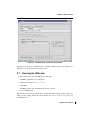
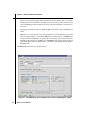
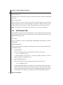
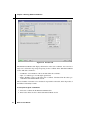
2. In the Potential tab, ensure that OPLS_2005 is selected in the Force field option menu, and
deselect Use non-bonded cutoffs (this stabilizes the minimization for this small receptor).
3. In the QM Optimization tab, ensure that Minimization is selected in the Method option
menu.
QSite 5.0 User Manual
5
Chapter 2: QSite Tutorial
Figure 2.1. The Potential tab of the QSite panel.
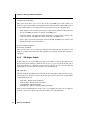
2.6
Defining a QM Region
You can select an isolated ligand molecule, a lone ion, or a metallic cofactor for the QM region
by simple picking. To select entire residues from protein chains, you must make backbone cuts
or use hydrogen caps. It is often useful to make side chain cuts, adding only the side chain
rather than the entire residue to the QM region. The following exercise demonstrates QM
region definition by ligand picking.
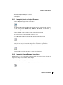
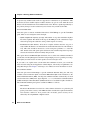
1. In the QM Region subtab of the QM Settings tab, ensure that the Pick option is selected.
2. Choose Free ligand/ion from the Pick option menu.
3. Pick an atom in the ligand.
Markers in cyan are superimposed on the ligand molecule to indicate that it has been
selected for the QM region. In the table, the type of cut and the name of the residue or ion
are listed. In this case, the name is the molecule number. The cyan color indicates that the
row for this cut is selected in the table.
6
QSite 5.0 User Manual
Chapter 2: QSite Tutorial
Figure 2.2. The QM Settings tab with the ligand picked.
QM region size is the most influential factor in QSite calculation speed. It is therefore not
advantageous to work with smaller model proteins.
2.7
Running the QSite Job
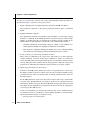
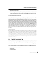
1. In the lower left corner of the QSite panel, click Start.
The QSite - Start dialog box is displayed.
2. Change the job name to qsite_tutorial.
3. Click Start.
The Monitor panel opens and displays the job log as it runs.
4. Close the QSite panel.
This job runs for several hours. If you wish to examine the results without waiting for the job to
finish, you may simply import the output structure file, qsite-1tpb.01.mae, from your
working directory.
QSite 5.0 User Manual
7
Chapter 2: QSite Tutorial
Figure 2.3. The QSite - Start dialog box.
The following files appear in your current Maestro working directory (qsite-workdir) before
the job starts:
qsite_tutorial.in
QSite input file
qsite_tutorial.mae
Maestro structure file
When the job is complete, these files are written:
qsite_tutorial.out
QSite output file
qsite_tutorial.log
Log file as displayed in the Monitor panel
qsite_tutorial.01.in
QSite restart file
qsite_tutorial.01.mae
Maestro structure file with optimized structure
2.8
Examining Results
In the next two exercises, you will examine the results of the calculation. If you decided not to
run the job, you can import the results from your working directory, as follows:
1. Click the Import structures toolbar button.
The Import panel is displayed.
2. Choose Maestro from the Format menu.
3. Select the file qsite-1tpb.01.mae.
8
QSite 5.0 User Manual
Chapter 2: QSite Tutorial
4. Ensure that Replace Workspace is selected.
5. Click Import.
2.8.1
Comparing Input and Output Structures
1. Click the Open/Close project table toolbar button
The Project Table panel opens. The output structure has been appended to the project as
an entry, with properties QM/MM Energy, QM Basis, QM Method, and Job Name. By
default, the output structure is included in the Workspace.
2. Control-click the check box in the In column for the original structure.
The original structure is included in the Workspace as well.
3. Choose Molecule Number from the Color all atoms by scheme button menu
f
Each of the four molecules in the Workspace (two receptors and two ligands) is now distinctly colored, and you can see what changes have occurred in the optimization.
4. Choose Element from the Color all atoms by scheme toolbar button menu.
Corresponding atoms in the two entries are now colored identically.
2.8.2
Comparing Ligand-Receptor Interactions
In this exercise you will compare the hydrogen bonding interactions between ligand and
receptor in the input complex and the output complex.
1. Include only the input entry in the Workspace.
2. Choose Inter H-Bonds from the Display H-bonds toolbar button menu.
QSite 5.0 User Manual
9
Chapter 2: QSite Tutorial
Figure 2.4. Input structure: ligand-receptor hydrogen bonds.
Figure 2.5. Output structure: ligand-receptor hydrogen bonds.
10
QSite 5.0 User Manual
Chapter 2: QSite Tutorial
3. Pick the ligand molecule.
Hydrogen bonds between the ligand and nearby receptor residues are shown as dashed
yellow lines, as shown in Figure 2.4.
4. Control-click the In check box for the output entry. Both entries are now included.
5. Control-click the In check box for the input entry to exclude it.
Using control-click to include and exclude entries allows the definitions of the molecules
to display H-Bonds for to stay the same.
In the output structure, notice that the hydrogen bond between LYS 13 and the ligand has been
lost, while two new hydrogen bonds have formed between ASP 165 and the ligand’s hydroxamate group (Figure 2.5). You might have to rotate the structures to locate a good view of the
hydrogen bonds, as shown in the figures.
QSite 5.0 User Manual
11
12
QSite 5.0 User Manual
QSite User Manual
Chapter 3
Chapter 3:
Protein Preparation
The quality of QSite results depends on reasonable starting structures. Schrödinger offers a
comprehensive protein preparation facility in the Protein Preparation Wizard, which is
designed to ensure chemical correctness and to optimize protein and protein-ligand complex
structures for use as input. For QSite, the entire system (both MM and QM regions) must be
prepared so as to satisfy the requirements of Impact/OPLS_2001, while the QM region must
satisfy the requirements of Jaguar. It is strongly recommended that protein structures imported
from non-Maestro sources, such as PDB structures, be treated with the protein preparation
facility in order to achieve best results.
For the molecular mechanics simulations using Impact with OPLS force fields, structures must
be all-atom (explicit hydrogens) and there must be no covalent bonds between ligand atoms
and protein atoms, including protein metal atoms. Bond orders and formal charges must be
correct.
For Jaguar calculations on the QM region, structures must be three-dimensional and correct
(have reasonable starting bond orders and formal charges).
3.1
Protein Preparation Procedure
A typical PDB structure file consists only of heavy atoms, can contain waters, cofactors, and
metal ions, and can also be multimeric. The structure generally has no information on bonding
or charges. Terminal amide groups can also be misaligned, because the X-ray structure analysis cannot usually distinguish between O and NH2. For QSite calculations, which use an allatom force field, atom types and bond orders must be assigned, the charge and protonation
states must be corrected, side chains reoriented if necessary, and steric clashes relieved.
This section provides an overview of the protein preparation process. The entire procedure can
be performed in the Protein Preparation Wizard panel, which you open from the Workflows
menu on the main toolbar. This tool and its use is described in detail in Chapter 2 of the Protein
Preparation Guide.
After processing, you will have files containing refined, hydrogenated structures of the ligand
and the ligand-receptor complex. The prepared structures are suitable for use with QSite. In
most cases, not all of the steps outlined need to be performed. See the descriptions of each step
to determine whether it is required.
QSite 5.0 User Manual
13
Chapter 3: Protein Preparation
You may on occasion want to perform some of these steps manually. Detailed procedures are
described in Chapter 3 of the Protein Preparation Guide.
1. Import a ligand/protein cocrystallized structure, typically from PDB, into Maestro.
The preparation component of the protein preparation facility requires an identified
ligand.
2. Simplify multimeric complexes.
For computational efficiency it is desirable to keep the number of atoms in the complex
structure to a minimum. If the binding interaction of interest takes place within a single
subunit, you should retain only one ligand-receptor subunit to prepare for QSite. If two
identical chains are both required to form the active site, neither should be deleted.
• Determine whether the protein-ligand complex is a dimer or other multimer containing duplicate binding sites and duplicate chains that are redundant.
• If the structure is a multimer with duplicate binding sites, remove redundant binding
sites and the associated chains by picking and deleting molecules or chains.
3. Locate any waters you want to keep, then delete all others.
These waters are identified by the oxygen atom, and usually do not have hydrogens
attached. Generally, all waters (except those coordinated to metals) are deleted, but
waters that bridge between the ligand and the protein are sometimes retained. If waters
are kept, hydrogens will be added to them by the preparation component of the protein
preparation job. Afterwards, check that these water molecules are correctly oriented.
4. Adjust the protein, metal ions, and cofactors.
Problems in the PDB protein structure may need to be repaired before it can be used.
Incomplete residues are the most common errors, but may be relatively harmless if they
are distant from the active site. Structures that are missing residues near the active site
should be repaired.
For the MM calculations, metal ions in the protein complex cannot have covalent bonds
to protein atoms. The MacroModel atom types for metal ions are sometimes incorrectly
translated into dummy atom types (Du, Z0, or 00) when metal-protein bonds are specified
in the input structure. Furthermore, isolated metal ions may erroneously be assigned general atom types (GA, GB, GC, etc.).
Cofactors are included as part of the protein, but because they are not standard residues it
is sometimes necessary to use Maestro’s structure-editing capabilities to ensure that multiple bonds and formal charges are assigned correctly.
• Fix any serious errors in the protein.
14
QSite 5.0 User Manual
Chapter 3: Protein Preparation
• Check the protein structure for metal ions and cofactors.
• If there are bonds to metal ions, delete the bonds, then adjust the formal charges of
the atoms that were attached to the metal as well as the metal itself.
• Set charges and correct atom types for any metal atoms, as needed.
• Set bond orders and formal charges for any cofactors, as needed.
5. Adjust the ligand bond orders and formal charges.
If the complex structure contains bonds from the ligand or a cofactor to a protein metal,
they must be deleted. Impact models such interactions as van der Waals plus electrostatic
interactions. Impact cannot handle normal covalent bonds to the ligand, such as might be
found in an acyl enzyme.
If you are working with a dimeric or large protein and two ligands exist in two active
sites, the bond orders have to be corrected in both ligand structures.
6. Run a restrained minimization of the protein structure.
This is done with impref, and should reorient side-chain hydroxyl groups and alleviate
potential steric clashes.
7. Review the prepared structures.
• If problems arise during the restrained minimization, review the log file, correct the
problems, and rerun.
• Examine the refined ligand/protein/water structure for correct formal charges, bond
orders, and protonation states and make final adjustments as needed.
3.2
Checking the Protein Structures
After you have completed the protein preparation, you should check the completed ligand and
protein structures.
3.2.1
Checking the Orientation of Water Molecules
You only need to perform this step if you kept some structural waters. Reorienting the hydrogens is not strictly necessary, as their orientation should have been changed during refinement,
but it is useful to check that the orientation is correct.
If the orientation is incorrect, reorient the molecules by using the procedure outlined in
Section 3.9 of the Protein Preparation Guide.
When you have corrected the orientation of the retained water molecules, you should run a
refinement on the adjusted protein-ligand complex.
QSite 5.0 User Manual
15
Chapter 3: Protein Preparation
3.2.2
Checking for Steric Clashes
You should make sure that the prepared site accommodates the co-crystallized ligand in the
restraint-optimized geometry obtained from the structure preparation.
Steric clashes can be detected by displaying the ligand and protein in Maestro and using the
Contacts folder in the Measurements panel to visualize bad or ugly contacts. Maestro defines
bad contacts purely on the basis of the ratio of the interatomic distance to the sum of the van
der Waals radii it assigns. As a result, normal hydrogen bonds are classified as bad or ugly
contacts. By default, Maestro filters out contacts that are identified as hydrogen bonds, and
displays only the genuine bad or ugly contacts.
If steric clashes are found, repeat the restrained optimization portion of the protein preparation
procedure, but allow a greater rms deviation from the starting heavy-atom coordinates than the
default of 0.3 Å. Alternatively, you can apply an additional series of restrained optimizations to
the prepared ligand-protein complex to allow the site to relax from its current geometry.
3.2.3
Resolving H-Bonding Conflicts
You should look for inconsistencies in hydrogen bonding to see whether a misprotonation of
the ligand or the protein might have left two acceptor atoms close to one another without an
intervening hydrogen bond. One or more residues may need to be modified to resolve such an
acceptor-acceptor or donor-donor clash.
Some of these clashes are recognized by the preparation process but cannot be resolved by it.
The preparation process may have no control over other clashes. An example of the latter typically occurs in an aspartyl protease such as HIV, where both active-site aspartates are close to
one or more atoms of a properly docked ligand. Because these contact distances fall within any
reasonable cavity radius, the carboxylates are not subject to being neutralized and will both be
represented as negatively charged by the preparation process. However, when the ligand interacts with the aspartates via a hydroxyl group or similar neutral functionality, one of the aspartates is typically modeled as neutral.
If residues need to be modified, follow these steps:
1. Place the refined protein-ligand complex in the Workspace.
2. Examine the interaction between the ligand and the protein (and/or the cofactor).
3. Use your judgment and chemical intuition to determine which protonation state and tautomeric form the residues in question should have.
4. Use the structure-editing capabilities in Maestro to resolve the conflict (see Section 3.8 of
the Protein Preparation Guide for procedures).
16
QSite 5.0 User Manual
Chapter 3: Protein Preparation
5. Re-minimize the structure.
It is usually sufficient to add the proton and perform about 50 steps of steepest-descent minimization to correct the nearby bond lengths and angles. Because this optimizer does not make
large-scale changes, the partial minimization can be done even on the isolated ligand or protein
without danger of altering the conformation significantly. However, if comparison to the original complex shows that the electrostatic mismatch due to the misprotonation has appreciably
changed the positions of the ligand or protein atoms during the protein-preparation procedure,
it is best to reprotonate the original structure and redo the restrained minimization.
QSite 5.0 User Manual
17
18
QSite 5.0 User Manual
QSite User Manual
Chapter 4
Chapter 4:
Running QSite From Maestro
QSite performs mixed quantum mechanical/molecular mechanical (QM/MM) calculations,
using Jaguar for the QM calculations and Impact for the MM calculations. Ligands and other
specified regions of a protein complex can be studied using QM, while MM is used for the rest
of the molecule.
At each step of a QM geometry optimization, Impact calculates energy terms for MM-QM
region interactions; if MM minimization was also specified, it is also performed at each QM
step. The next QM step takes into account the new MM atom distribution and energy terms. If
a single-point QM calculation is selected, the current QM/MM energy is calculated without
MM minimization.
The speed of QSite is largely determined by the size of the QM region. Therefore there is no
advantage to making a smaller model protein. You can run calculations on systems with up to
than 8000 atoms or 8000 bonds from the QSite panel, but larger systems must be run them
from the command line. See Section 4.10 on page 43 for more information.
Cartesian constraints may be placed on atoms in both the QM and the MM regions. See
Section 4.4 on page 31 for a description of the two types of constraints. Frozen-atom
constraints can be applied to atoms in both regions. Constrained atoms can be specified for
MM-region atoms, but are ignored if applied to QM-region atoms.
In general, a QSite calculation can only be performed using a single entry. If you want to run a
QSite job using the Workspace structure as input, and that structure includes multiple entries,
combine them into a single entry using the Merge option from the Entry menu in the Project
Table panel. The merged entry should be the only entry included in the Workspace when you
start the job. One exception to this is when setting up a transition-state search. In this case you
may select up to three Project Table entries, depending upon the algorithm that is selected for
performing the search. See Section 4.7 for more information about transition-state searching.
4.1
The QSite Panel
QSite calculations can be set up and run using the QSite panel. To open the QSite panel, choose
QSite from the Applications menu.
At the top of the panel is an option menu for selecting the source of structure input, which is
described in the next subsection. The center section of the panel has six tabs:
QSite 5.0 User Manual
19
Chapter 4: Running QSite From Maestro
•
•
•
•
•
•
QM Settings—specify the QM region and other QM options.
Potential—choose settings for the MM potential energy function.
MM Constraints—set up atom constraints for atoms in the MM region.
QM Constraints—set up constraints for atoms in the QM region.
MM Minimization—set up energy minimization of the MM region.
QM Optimization—select and set up the job task.
These tabs are described in later sections of this chapter. Below the tabs are several action
buttons, which are described in a subsection below.
4.1.1
Source of Structure Input
Input for QSite single point jobs, minimization jobs, and standard transition state searches
must be a single Project Table entry. To use a system consisting of two or more entries as the
input, choose Merge from the Entry menu in the Project Table panel, create a combined entry,
and run the simulation on that entry. LST and QST transition state searches are a special case:
here, the input is specified in the QM Optimization tab.
You can select the source of input from the Use structures from option menu. The options are
described below.
Workspace (included entry)
This is the default option. The structure that is currently included in the Workspace is used as
input to the job. This includes whatever atoms, molecules, or entries are part of the structure,
even atoms that have been undisplayed. You must choose this option if you want to use
constraints (see the Constraints tab, Section 4.4 on page 31), because the constraints are
applied to the Workspace structure.
Project Table (selected entry)
Select this option to use the entry that is currently selected in the Project Table. This may be
different from the structure in the Workspace. Because atom constraints are applied to the
Workspace structure, they are ignored if this option is chosen.
4.1.2
Action Buttons
The lower part of the QSite panels contains a row of action buttons. Apart from the standard
Close and Help buttons, for closing the panel and opening the help viewer, there are three
buttons for job-related actions, described below.
20
QSite 5.0 User Manual
Chapter 4: Running QSite From Maestro
Start
Click the Start button to open the Start dialog box. Section 4.10 describes how to start jobs
using the Start dialog box.
Read
The Read button reads a QSite input file and imports the associated structure. It opens a file
selector in which you can navigate to the desired input file.
Write
The Write button writes out all the files required for the job but does not run the job. Once the
files required for the job are written by Maestro, the job can be run from the command line in a
terminal window using the syntax:
$SCHRODINGER/qsite job-options jobname
where jobname.in is the input file for the job in question, and job-options is a list of options
for the job. The log output is written to jobname.log.
Type $SCHRODINGER/qsite for a usage summary of the qsite command, or see Chapter 5
for information on running QSite from the command line.
4.2
The QM Settings Tab
The QM Settings tab is used to enter information for the QM job and to define the QM region.
QM job information includes the quantum-mechanical method to be used, the charge and spin
multiplicity of the QM system, and other keywords and options that may be required by Jaguar.
The QM region can be defined by one of the following methods:
• Selecting the ligand, metal ions, or other disconnected species (not covalently bonded to
the protein).
• Specifying cuts between certain covalently-bonded atoms in connected peptide residues.
QSite cuts are specially parameterized frozen-orbital boundaries between the QM and
MM regions. They can be placed between an alpha carbon and a side chain (side-chain
cuts) or between an alpha carbon and the backbone to one side (backbone cuts, which
must be made in pairs to add the residues between them to the QM region).
In QSite 5.0, QSite cuts are parametrized to the OPLS_2001 force field. However, you
can use either the OPLS_2001 or the OPLS_2005 force field for calculations.
QSite 5.0 User Manual
21
Chapter 4: Running QSite From Maestro
Cuts in a protein-ligand complex must be between atoms in peptide residues. Covalentlybound ligands can be included in the QM region, but only along with attached protein
atoms. The QM region must extend at least as far as the first permissible cut between protein atoms.
• Specifying cuts between atoms for which the QM region will be capped with hydrogen
atoms.
Hydrogen caps can be placed on any atom designated to be in the QM region, provided
that it is singly-bonded to an atom in the MM region, and that any two such MM atoms
are separated in the MM region by at least three bonds. This option offers much more
flexibility in the selection of the QM region. The MM atom is replaced with a hydrogen
atom in the QM calculation, which leaves a chemically well-defined structure with no
dangling bonds.
The QM Settings tab features are described below.
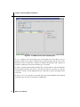
Figure 4.1. The QM Settings tab of the QSite panel, showing the QM Region subtab.
22
QSite 5.0 User Manual
Chapter 4: Running QSite From Maestro
4.2.1
General Settings
Method
The options for the QM method include several density functional theory methods (DFTB3LYP, DFT-PWB6K, DFT-M06, DFT-M06-2X, DFT-M06-L, DFT-M06-HF, DFT-M05, DFT-M052X), Hartree-Fock (Hartree-Fock), and local Møller-Plessett perturbation theory (Local MP2).
The DFT-User defined option is selected when an input file is read that specifies a functional
other than those available from this menu. Otherwise this option is not available. For more
information on the functionals, see Section 3.3 of the Jaguar User Manual.
Spin-unrestricted option
Select this option to perform a spin-unrestricted open-shell calculation. This option is only
available with the Hartree-Fock and DFT-B3LYP methods. Otherwise, open-shell calculations
will be performed with the restricted open-shell methods.
Charge
This is the net charge of the QM region of the system. Maestro updates the charge to a reasonable value whenever a new residue or ion is added to the QM region. If a discrepancy appears,
edit the value. If this value does not match the sum of the formal charges of the atoms in the
QM region, Maestro displays a warning message, but allows you to proceed.
Multiplicity
Check that this is the associated spin multiplicity of the QM region of the system: 1 for singlet,
2 for doublet, etc. Edit the value if necessary. If there is a discrepancy between the total charge
and the multiplicity, the Jaguar calculation will halt with an error message. The charge and
multiplicity of the QM region must be mutually consistent. By default, open-shell calculations
are spin-restricted. If you want to perform a spin-unrestricted HF or DFT calculation, you can
select the Spin-unrestricted option.
QM options
This text box can contain any Jaguar keywords such as print settings, non-default convergence
criteria, and so on. Each such option is of the form keyword=value (with no embedded blanks).
Multiple keyword/value pairs can be specified, separated by one or more blank spaces. By
default, the following QM options appear in the box:
iacc=1 vshift=1.0 maxit=100
You can remove or modify these options as appropriate. See Chapter 8 of the Jaguar User
Manual for more information on Jaguar keywords.
QSite 5.0 User Manual
23
Chapter 4: Running QSite From Maestro
Hydrogen cap electrostatics
This option menu allows you to choose how atoms in the MM region in the vicinity of a
hydrogen cap are treated when calculating their electrostatic interaction with the QM region. It
is only available when you are using hydrogen caps to define part or all of the QM region.
• Point charges—Use modified point charges to represent the potential of the atoms near
the cap, and MM point charges for the rest of the MM region.
• Gaussian charges—Use Gaussian charge distributions to represent the potential of the
atoms near the cap, and MM point charges for the rest of the MM region.
• None—Ignore electrostatic interactions between the QM and MM regions entirely. Van
der Waals interactions are still included.
Use wave function in input file
Use Hessian in input file
These options allow you to read the wave function and the Hessian from the input file, and
make use of them in the calculation. This capability is particularly useful when restarting a
calculation.
4.2.2
QM Region Subtab
In this subtab, you set up the QM region. The total number of atoms in the QM region is
displayed below this subtab. To define the region, choose a type of cut from the Pick option
menu, and pick atoms to define the cut. If you want to delete a cut, select it in the table and
click Delete. To start over with the selection of cuts, click Delete All.
QM region table
The cuts that define the QM region are listed in the table. The Type column gives the cut type,
and corresponds to the choice made from the Pick option menu to define the cut. The Name
column identifies the cut:
•
•
•
•
Side chain—Residue name and number
Entire residue—Residue name and number
Free ligand/ion—Molecule number
Hydrogen cap—QM atom=number, MM atom=number
When you have finished picking to define a cut or a set of QM atoms, table rows are added for
each cut or atom set. To delete a cut, select the cut in the table and click Delete.
24
QSite 5.0 User Manual
Chapter 4: Running QSite From Maestro
Pick option and menu
Select this option to pick the location of one or more cuts, and choose the type of cut from the
option menu. Note that a residue can be an amino acid residue, a free ligand or solvent molecule, or an ion. The items on the option menu are:
• Side chain
Choose this option to add only the side chain of an amino acid residue to the QM region,
leaving the backbone in the MM region. Pick an atom in the side chain you want to
include. The side chain is marked in sienna if Show markers is selected. A cut is made
between the alpha carbon and the beta carbon of that residue. All of the atoms in the side
chain are part of the QM region.
Side-chain cuts can be made in any peptide residue other than alanine (ALA), glycine
(GLY), and proline (PRO). To incorporate side chains from these residues in the QM
region, you must select the entire residue by using a backbone cut. Side-chain cuts can be
made in positively-charged histidine (HIP) as well. Side-chain cuts are not permitted if
the side chain has been modified within 3 atoms of the alpha carbon atom.
• Entire residue
To add entire amino acid residues to the QM region, choose this option and then pick two
atoms that are not alpha carbons and are at least three backbone bonds apart. The residues
containing these two atoms and the residues in between are included in the QM region.
The cut between MM and QM atoms is made between the alpha carbon and the backbone
atom bonded to it. When you pick the first atom it is marked with a purple cube. After
picking the second atom, all of the backbone and side chain atoms between the two cuts
are marked in sienna if Show markers is selected.
If you click twice on the same atom in an amino acid residue, then the QM/MM cuts will
be set as small as possible so as to place that entire residue in the QM region.
Backbone cuts can be made in any peptide residue, including glycine, proline, and their
adjacent residues, and including positively-charged histidine (HIP). There is one exception: backbone cuts on PRO residues cannot be made between the N atom and the Cα
atom.
There must be at least 3 bonds between pairs of QM-MM cuts that are made along the
protein backbone. This ensures that the QM/MM boundaries are kept far enough apart
that they do not interfere with one another. This means that the smallest QM region that
contains all of the atoms of an amino acid residue would necessarily contain an extra carbonyl group and an extra N-H bond from the neighboring residues.
QSite 5.0 User Manual
25
Chapter 4: Running QSite From Maestro
A backbone cut cannot be placed between an amino acid residue and an end cap. The end
cap must be included in the QM region. To do this you may click on any atom in an end
cap, and on any other atom in an amino acid residue further up the chain. In this case only
one cut will actually be made, and all atoms from the cut to the end of the chain will be
placed into the QM region.
The cuts made with this choice use the frozen-orbitals method for defining the terminus
of the QM region.
• Free ligand/ions
Entire free ligands, metal ions, or other species not covalently bound to the protein can be
added to the QM region by this method, which does not make any cuts between atoms.
Select this option, then pick a metal ion or an atom in the ligand molecule to add it to the
QM region. Molecules are marked in sienna, and single atoms or ions are marked in cyan,
if Show markers is selected.
Ligands that are covalently bound to the protein cannot be added using this method,
because this method does not make parametrized cuts between bonded atoms. To add
covalently-bound ligands to the QM region, make either a pair of backbone cuts to select
the residue to which the ligand is bound, or make a side-chain cut.
• Hydrogen cap
To define cuts that are capped by hydrogen atoms rather than atoms with frozen orbitals,
select this option and then pick the QM atom followed by the MM atom on either side of
the cut. The QM atom and the MM atom must be joined by a single bond. The MM atom
is replaced by a hydrogen atom in the QM calculation. The QM region usually requires
two or more cuts. The markers in the Workspace are not updated after making this kind of
cut. Instead, you must click Update QM Region Display to display the markers for the QM
region (provided Show markers is selected).
Once you have created a hydrogen cap, the Hydrogen cap electrostatics option menu in
the general section becomes available, and you can choose the electrostatic treatment of
MM atoms near the cap.
Show markers option
If this option is selected, markers are displayed in the Workspace to indicate the QM region.
Ball-and-stick markers are superimposed on the QM region atoms. The markers are colored
sienna. The markers that correspond to the selected rows in the QM region table are colored
cyan. For hydrogen caps, an arrow is superimposed on the bond where the cap will be placed,
pointing to the MM atom that will be replaced with a hydrogen atom.
26
QSite 5.0 User Manual
Chapter 4: Running QSite From Maestro
Figure 4.2. The QM Settings tab of the QSite panel, showing the QM Basis subtab.
4.2.3
QM Basis subtab
In this subtab you can view and change the basis set associated with each atom in the QM
region.
Basis set table
This table lists the basis set used for each QM atom. The atom is identified in the QM Atom
column, and the basis set used is given in the Basis column. You can select multiple rows and
apply a basis set to the selection.
Pick option and menu
Select this option to pick atoms for which you want to change the basis set. Three of the
options on the menu are the same as in the QM Region tab, and work in the same way. The
Hydrogen cap option is not present; instead there is an Atom option that enables you to pick
individual atoms. The atoms you pick are marked with green axes if Show markers is selected,
and they are also selected in the basis set table.
QSite 5.0 User Manual
27
Chapter 4: Running QSite From Maestro
Show markers option
When this option is selected, the atoms that are selected in the table or picked are marked with
green axes.
Basis set option menu
Choose the basis set for the selected rows in the basis set table from this option menu. By
default, the basis set used for the entire QM region is LACVP*, which uses 6-31G* for nontransition metals. This is the basis set used in the parameterization of the frozen orbital cuts.
Note:
4.3
The inclusion of frozen-orbital cuts enforces the use of 5D for the d functions.
The Potential Tab
The Potential tab provides options for the definition of the potential energy functions used in
the molecular mechanics part of the calculation. One of these (continuum solvation) affects the
QM potential energy as well.
Force Field
The two available force fields are OPLS_2001 and OPLS_2005. The default force field is
OPLS_2005.
Electrostatic treatment
This option menu offers two methods for calculating the electrostatic component of the molecular mechanics energy:
• Constant dielectric
This option calculates the electrostatic interaction between atoms i and j as:
Eele = 332.063762 qiqj/(ε rij)
A constant dielectric is appropriate for a vacuum (gas-phase) calculation or when an
explicit or implicit solvent model is used.
• Distance dependent dielectric
This option calculates the electrostatic interaction between atoms i and j as:
Eele = 332.063762 qiqj/ε rij2
A distance-dependent dielectric is sometimes used as a primitive model for the effect of
solvent. In this model, the electrostatic interaction between a pair of atoms falls off rapidly as the distance between the atoms increases. Continuum and explicit solvent models
are much better at accounting for solvent effects than a distance-dependent dielectric.
28
QSite 5.0 User Manual
Chapter 4: Running QSite From Maestro
Figure 4.3. The Potential tab of the QSite panel.
The variables in the above formulae are defined as follows:
•
•
•
•
Eele is the electrostatic interaction in kcal/mol
qi and qj are the partial atomic charges on atom i and j
rij is the distance in Å between atoms i and j
ε is the Dielectric constant (see below)
Dielectric constant
This text box specifies the value of the dielectric constant ε used in the electrostatic calculations.
In molecular-mechanics calculations it is often impractical to include the nonbonded (electrostatic and van der Waals) interactions between every pair of atoms. For large systems, many
such pairs are separated by a great distance and contribute little to the interaction energy. Judicious truncation of the non-bonded interactions between widely separated pairs of atoms is an
important strategy for reducing the resources needed for calculations on large systems.
QSite 5.0 User Manual
29
Chapter 4: Running QSite From Maestro
At present only residue-based cutoffs are supported for calculations set up in Maestro. This
means that all atoms within complete residues that have any pair of atoms within the cutoff
distance will be included in the non-bonded interaction list. The list is updated periodically as
the geometry changes, because residues may move inside or beyond the cutoff radius.
Use non-bonded cutoffs
Select this option to truncate nonbonded interactions. Click Settings to open the Truncation
panel. There are two settings that can be changed:
• Update neighbor-list frequency (# steps): The number of steps after which the neighbor
list will be updated. The default is 10 steps (in the MM part of the calculation). Larger
values will speed up the calculation, at the possible expense of accuracy.
• Residue-based cutoff distance: All atoms in complete residues that have any pair of
atoms within this distance are included in the nonbonded interaction list. The default is
12 Å. This value should be increased to avoid convergence problems, to a value like
30 Å. Smaller values will speed up the calculations, but could miss important long-range
electrostatic interactions between formally charged atoms.
This option affects both MM and QM calculations. Do not select Use continuum solvation if
you intend to run the QM (Jaguar) calculation using multiple processors (parallel processing);
when QSite jobs with solvation are run in parallel, erroneous energies result.
If you want to use explicit water solvent rather than continuum solvation, you can add the
water molecules using the Soak application of Basic Impact, followed by an equilibration, also
using Basic Impact. See Chapter 5 of the Impact User Manual for more information on Soak.
Use continuum solvation
Select this option and click Settings to open the Continuum Solvation dialog box. The only
available solvation method in QSite, for both the MM and the QM solvation functions, is the
Poisson–Boltzmann Solver (PBF); selecting Use continuum solvation automatically sets both
solvation functions to PBF (in the Jaguar input file, isolv=2). The Surface Generalized Born
(SGB) and Analytic Generalized Born (AGB) methods are not available for QSite calculations.
The Continuum Solvation panel options available for PBF are as follows:
• PBF resolution
The Poisson–Boltzmann solver involves a finite-element calculation on a grid. The grid
spacing controls the accuracy of the PBF calculation and the time required. The default,
Low resolution, suffices for most protein work. If needed, greater accuracy can be
achieved by choosing Medium or High resolution.
30
QSite 5.0 User Manual
Chapter 4: Running QSite From Maestro
• PBF displacement threshold
This text box specifies how far (in Å) any atom may move from the coordinates used in
the previous PBF calculation before a new PBF calculation must be performed. If no
atom has moved this distance, the previously calculated PBF energy and forces are used.
Use atomic partial charges in structure file
With this option, you can choose to use the atomic partial charges that are stored in the input
structure file, rather than the partial charges that are assigned by the force field.
This option should only be used when the QM region consists of one or more non-covalently
bound molecules. If you use this option for a system in which you make frozen orbital cuts or
hydrogen caps, the resulting structure and properties will generally be erroneous. The handling
of frozen orbitals involves a parameterization for the potential about the frozen bond, which
relies on particular values for the partial charges of the atoms near the QM/MM interface. In
general the charges in the Maestro structure file will not be appropriate for use with frozen
orbitals. ESP charges written to the output Maestro file from jobs with frozen orbitals or
hydrogen caps are only for the QM atoms and will not usually add up to the appropriate molecular charge.
Skip force field checks
By default, Impact performs a number of tests during atom typing to guide selection of optimal
force-field parameters for the atoms in the input structure. The tests are applied to both the MM
and the QM regions. For transition metals, force-field parameters are more limited than for the
common p-block elements, so when the structure contains transition metals, these atom typing
tests can fail and cause the job to halt. The force field is not used if the metals are in the QM
region. By selecting this option, the force-field checks are bypassed, and the metal atoms do
not cause the job to fail.
4.4
The MM Constraints Tab
The MM Constraints tab is used to apply constraints to the Cartesian coordinates of selected
atoms in the MM region. Specified atoms can be frozen at their input coordinates (frozen-atom
constraints), or they can be constrained to remain near their initial coordinates by applying a
harmonic force.
Atom constraints in QSite for atoms in the MM region must be set in the MM Constraints tab.
The Constraints tab contains two buttons:
• Frozen Atoms
• Constrained Atoms
QSite 5.0 User Manual
31
Chapter 4: Running QSite From Maestro
Figure 4.4. The MM Constraints tab of the QSite panel.
These buttons open the Frozen Atoms and Constrained Atoms panels. These panels have a
similar structure. The panel features are described below.
Atoms list
The upper portion of each panel is a text area that lists the atom number of each atom that has
been selected to be frozen or constrained. The currently selected atom is highlighted.
Picking tools
This section, labeled Define Frozen Atoms or Define Constrained Atoms, contains standard
picking controls: a Pick check box and menu, which is set to Atoms by default; an All button; a
Select button, which opens the Atom Selection dialog box. If you deselect the Pick check box,
you can use the Workspace selection tool to select atoms, then click the Selection button to add
those atoms to the list, or use the Previous button to return to the most recent selection.
The picking tools section also contains a Show markers option, which is selected by default.
Atoms to be frozen are marked with a red cross and a “padlock” icon in the Workspace. Atoms
to be constrained are marked with a brown cross and a “spring” icon in the Workspace display.
32
QSite 5.0 User Manual
Chapter 4: Running QSite From Maestro
Figure 4.5. The Constrained Atoms panel.
To distinguish the currently selected frozen or constrained atom, Maestro colors the marker
turquoise.
Constraining force
The Constraining force text box sets the value of the harmonic force constant applied to the
selected constrained atoms. The same force constant is used for all atoms. The default is
25.00 kcal/(mol Å2).
Deletion buttons
The constraint on the currently selected atom can be removed by clicking Delete. The atom is
then removed from the atoms list. To remove all constraints of this type, click Delete All. The
atoms list is then cleared.
4.5
The QM Constraints Tab
The QM constraints tab is used to set constraints on geometric parameters in the QM region. It
provides the same capabilities as in the Optimization tab of the Jaguar panel. For full details,
see Section 4.2 of the Jaguar User Manual. Briefly, you can set constraints on distances,
angles, and dihedrals, and set Cartesian constraints. These constraints freeze the internal or
Cartesian coordinates. For Cartesian coordinates, you can only freeze the entire atom, not individual coordinates. You can also make constraints dynamic, which means that the optimization
will constrain the parameter to reach the target value specified at convergence. Harmonic
constraints are not available in the QSite panel, but can be set by using Jaguar keywords.
QSite 5.0 User Manual
33
Chapter 4: Running QSite From Maestro
Figure 4.6. The QM Constraints tab of the QSite panel.
To set a constraint, choose the parameter type from the Type menu, select Pick (if it is not
already selected), choose Atoms or Bonds from the Pick menu, then pick the atoms in the
Workspace for the constraint. The constraints are marked in the Workspace with a spring icon
and lines to indicate the atoms involved and the type of constraint.
To make a constraint in the Constraints table dynamic, select the table row, then select Dynamic
in the Selected constraint section next to the table and enter the value that you want the
constraint to converge on in the Target value text box. This value is copied to the Target column
of the table.
To delete one or more constraints, select them in the table and click Delete in the Selected
constraint section. To delete all constraints, click Delete All.
34
QSite 5.0 User Manual
Chapter 4: Running QSite From Maestro
4.6
The MM Minimization Tab
The MM Minimization tab specifies settings for Impact energy minimization of the MM region
of the molecule. If the QM method chosen in the Optimization tab is Single point, these settings
are not used, and no MM minimization is performed. The options available in this tab are
described below.
Maximum cycles
Set the maximum number of cycles for the minimization calculation in this text box. The minimization terminates if it has not converged by this point. The default value of this setting is 100
iterations, but you can specify any value greater than or equal to zero. “Zero cycles” is a special
case; it instructs Impact just to evaluate the energy for the current coordinates.
Algorithm
Choose the minimization algorithm from this option menu. The choices are:
• Truncated Newton (TN). This is a very efficient method for producing optimized structures. A short conjugate gradient pre-minimization stage is performed first to help
improve the convergence of the Truncated Newton algorithm.
• Conjugate gradient. This is a good general optimization method and is the default
method.
• Steepest descent. This can be a good method for initiating a minimization on a starting
geometry that contains large steric clashes. Convergence is very poor towards the end of
minimization, where the conjugate gradient algorithm should be used.
Initial step size
Specifies the initial step size of the minimization cycle for conjugate gradient and steepest
descent minimizations in this text box. The default value is 0.05, but any positive value is
allowed.
Maximum step size
Specify the maximum step size of the minimization cycle for conjugate gradient and steepest
descent minimizations in this text box. If the step size exceeds this value, the minimization will
halt. The default value is 1.00 Å, but any positive value is allowed. The maximum step size is
the maximum displacement allowed for an atom in any step of a minimization calculation.
QSite 5.0 User Manual
35
Chapter 4: Running QSite From Maestro
Figure 4.7. The MM Minimization tab of the QSite panel.
Convergence criterion
Choose the quantities used for the convergence criteria from this option menu. Either or both
of two criteria—energy change and gradient—can be specified. The options control the availability of the Energy change criterion and Gradient criterion text boxes.
Energy change criterion
Specify the value of the energy change criterion in this text box. The default value is 10-7 kcal/
mol, but any positive value is allowed. The criterion is satisfied if two successive energies
differ by less than the specified value.
Gradient criterion
Specify the value of the gradient criterion in this text box. The default value is 0.01 kcal/
(mol Å), but any positive value is allowed. The criterion is satisfied if the norms of two successive gradients differ by less than the specified value.
36
QSite 5.0 User Manual
Chapter 4: Running QSite From Maestro
Update long range forces every n steps.
Specify the frequency with which long range forces are updated for Truncated Newton minimizations in this text box. Between these intervals, estimates of these forces are used. Every 10
steps is the default; smaller numbers (more frequent updates) can be used to improve convergence, but will make the optimization slower. Larger numbers for n may speed the calculation,
but the maximum recommended value is 20.
Long range force cutoff > d Angstroms.
Specify the distance beyond which forces are considered long range, and are therefore updated
every n steps, for Truncated Newton minimizations in this text box. The default value is
10.0 Å.
4.7
The QM Optimization Tab
The QM Optimization tab specifies the type of QM (Jaguar) calculation to be performed and
provides information needed to set up the calculation. For transition state optimizations additional structures (reactant, product, and transition state guess structures) can be given to guide
the search. QSite geometry optimizations use internal coordinates by default; to force Cartesian coordinate optimization, run QSite from the command line, using the option intopt=0 in
the gen section of the Jaguar input file. The options available in this tab are described in the
following sections.
4.7.1
Calculation Type
The Method menu controls the QM calculation type. The options are:
• Single point—Calculate the QM energy for the structure as it stands. No QM geometry
optimization or MM minimization is performed. When Single point is selected, other
options in this tab are unavailable. Settings in the Minimization and Constraints tabs are
ignored. This is the default QM method.
• Minimization—Locate a minimum-energy structure by geometry optimization. If you
want to optimize only the QM region, simply set the number of minimization steps to 0 in
the Minimization tab. There is no need to explicitly freeze all of the MM atoms.
• Transition state—Locate a transition state structure by geometry optimization. The
remaining controls in the tab define the initial guess for the transition state geometry, and
are described in the next subsection.
For minimization and transition-state calculations, you can specify the number of optimization
iterations in the Maximum number of iterations text box. The default is 100 iterations.
QSite 5.0 User Manual
37
Chapter 4: Running QSite From Maestro
Figure 4.8. The QM Optimization tab with TS method: LST selected
4.7.2
Transition State Searches
If you select Transition state from the Method menu, the default option for TS method is Standard. The following three methods for transition-state optimization are supported in QSite,
corresponding to well-known ab initio techniques. See Section 4.3 of the Jaguar User Manual
for detailed information about these methods:
• Standard: The standard transition-state optimization method is useful if you have only a
single initial guess structure (the structure in the Workspace) for the transition-state. It
attempts to find the saddle point closest to the starting structure by maximizing the energy
along the lowest-frequency mode of the Hessian and minimizing the energy along all
other modes.
• LST: Linear Synchronous Transit is useful if you have initial guess structures for the reactant and the product and want QSite to look for a transition-state structure by interpolating between them. LST uses a quasi-Newton method to search for the optimum
transition-state geometry, choosing a transition-state guess structure based on the interpolation value you set using the Fraction of path between reactant and product slider. By
38
QSite 5.0 User Manual
Chapter 4: Running QSite From Maestro
default it is set at 0.50, directing QSite to choose an interpolated transition-state guess
structure midway between the reactant and the product. If you want to pick a guess structure closer to the reactant, move this slider toward 0.00. For a guess structure closer to the
product, move the slider toward 1.00
• QST: Quadratic Synchronous Transit is useful if you have initial guess structures for the
reactant, the product, and the transition state. QST uses a quasi-Newton method to optimize the transition-state geometry.
The structures that define the transition state initial guess can be specified in the Reactant
entry, Product entry, and TS guess entry sections. You can select the entry by typing in the
entry name from the Project Table, by clicking Choose and selecting the entry from a list, or, if
the structure is in the Workspace, by selecting Pick to define entry and clicking on any atom in
the structure.
4.8
The Surfaces Tab
In this tab, you can set options to generate electrostatic potential, electron density, spin density,
and molecular orbital surfaces at the end of the QSite job.
When you request molecular orbital surfaces, any frozen orbitals (from frozen-orbital cuts) are
ignored. If, for example, you request a surface for the HOMO, the surface is generated for the
highest-energy occupied orbital that is not frozen.
The options available in this tab are described below.
Electrostatic potential
Calculate the electrostatic potential (ESP) on the grid1. The units used to represent the ESP can
be selected from the ESP units option menu2.
Electron density
Calculate the electron density on the grid3.
Spin density
Calculate the electron spin density on the grid4 (sets iplotden=1 in the gen section). Only
available for UHF and UDFT wave functions.
1.
2.
3.
4.
Sets iplotesp=1 in the gen section
Sets espunit in the gen section
Sets iplotden=1 in the gen section
Sets iplotspn=1 in the gen section
QSite 5.0 User Manual
39
Chapter 4: Running QSite From Maestro
Figure 4.9. The Surfaces tab
Molecular orbitals
Calculate the specified molecular orbitals on the grid5. Not available for MP2 calculations. To
specify the desired orbitals, choose the references for the molecular orbital indices from the
From and to option menus and enter the relative index in the text box. The option menu choices
are:
• HOMO -: Count down from the HOMO, inclusive.
• LUMO +: Count up from the LUMO, inclusive.
Thus, From: HOMO - 0 to: LUMO + 0 includes both the HOMO and the LUMO. The controls
for beta orbitals are only available for UHF and UDFT wave functions.
Box size adjustment
Enter a value to adjust the size of the box used to calculate the grid6. The default box size
encompasses the van der Waals radii of all atoms in the molecule.
5.
6.
40
Sets iorb1a, iorb2a, iorb1b, iorb2b in the gen section
Sets xadj, yadj, zadj in the gen section
QSite 5.0 User Manual
Chapter 4: Running QSite From Maestro
Grid density
Enter the number of grid points per angstrom7.
4.9
The Scan Tab
In this tab, you set up the coordinates for a relaxed or a rigid coordinate scan. Whether the scan
is relaxed or rigid depends on the method selection in the QM Optimization tab: selecting Single
point from the Method option menu performs a rigid scan, selecting Minimization performs a
relaxed scan.
To add a new scan coordinate:
1. Choose a coordinate type from the Type option menu
2. Choose Atoms or Bonds from the Pick option menu
3. Pick the atoms or bonds in the Workspace.
The order of picking of the coordinates determines which atoms are moved in the scan: the last
atom picked is the moving atom, and the first atom picked remains stationary. If you are
picking bonds, they must be contiguous. The last atom (the moving atom) is the atom in the
last bond picked that is not part of the previous bond picked.
The choice you make from the Type option menu determines the number of atoms to pick. The
Z-matrix must be in the appropriate form for the coordinate type: Cartesian for Cartesian coordinates, and Z-matrix for distances, angles, and dihedrals. The coordinate types are:
•
•
•
•
Cartesian-X—X coordinate of an atom. Pick one atom.
Cartesian-Y—Y coordinate of an atom. Pick one atom.
Cartesian-Z—Z coordinate of an atom. Pick one atom.
Distance—Distance between two atoms. Pick two atoms or one bond. If you pick atoms,
they need not be bonded to each other.
• Angle—Angle between three atoms. Pick three atoms or two bonds. If you pick atoms,
they need not be bonded to each other.
• Dihedral—Dihedral angle between four atoms. Pick four atoms or three bonds. If you
pick atoms, they need not be bonded to each other.
The choices available on the Pick option menu are Atom for Cartesian coordinates, and Atom
and Bond for all other types of coordinates. The atoms are marked in the Workspace as you
pick them, and each coordinate is marked in the Workspace and entered in the Defined coordinates table as it is completed. If you want to select a protein dihedral angle, click Select. A
dialog box is displayed, in which you can select a standard dihedral from a list.
7.
Sets plotres in the gen section
QSite 5.0 User Manual
41
Chapter 4: Running QSite From Maestro
Figure 4.10. The Scan tab
The Defined Coordinates table displays information on the scan coordinates. You can select a
single row to define the range and point spacing for the coordinate in the Selected Coordinate
section. The table columns are:
• Coordinate—Atom numbers of the atoms that define the coordinate.
• Type—Coordinate type, from the Type option menu.
• Steps—Number of steps to take in the given coordinate. Calculated from the values provided in the Selected Coordinate section.
The total number of structures to be calculated is reported below the table, and is the product of
the numbers in the Steps column.
To set up the range for a coordinate:
1. Select the coordinate in the Defined coordinates table
2. Enter values in the text boxes in the Selected coordinate section.
42
QSite 5.0 User Manual
Chapter 4: Running QSite From Maestro
In the Selected Coordinate section , you can set the range of the scan and the spacing of the
points along the scan coordinate for the coordinate that is selected in the table. These values
are used to calculate the number of steps. The text boxes are described below.
•
•
•
•
•
Current value—Current value of the coordinate in the input structure. Noneditable.
Starting value—Initial value of the coordinate for the scan.
Final value—Final value of the coordinate for the scan.
Increment—Amount by which the coordinate is incremented at each scan step.
Number of steps—Number of steps to take in the given coordinate. Calculated from the
initial and final values and the increment.
You can delete coordinates by selecting them in the table and clicking Delete in the Selected
coordinate section.
4.10 Running QSite Jobs
When you have set the options in the QSite panel tabs to the desired value, click the Start
button to open the Start dialog box. In this dialog box you can set up the job options, then
submit the job to a host for execution. For details of the features of this dialog box, see
Section 4.2 of the Job Control Guide. When choosing job and host options, you should take
note of the following points:
• QSite does not automatically assign new names to jobs or files. If files of the same name
exist, a warning is displayed before any files are overwritten.
• You can use multiple CPUs for parallel processing of the QM part of the calculation, if
the host has multiple processors.
• Do not use parallel processing for jobs that include continuum solvation treatment, as
they will fail if you do.
When you have selected job options, click the Start button to run the job. QSite jobs can be
monitored in the job Monitor panel.
If a QSite job needs to be restarted, it can be restarted from Maestro or from the command line.
To restart a job from the command line, simply run QSite with the restart file specified as the
input:
$SCHRODINGER/qsite job-options jobname.01
The restart input file has an index number inserted into the file name: for the first restart it is
jobname.01.in. Running with this file produces a restart file named jobname.02.in, and so
on. Likewise, the output structure file has an index number inserted into the file name: for the
first job it is jobname.01.mae. The index number is the same as for the restart file.
QSite 5.0 User Manual
43
Chapter 4: Running QSite From Maestro
To restart a job from Maestro, open the QSite panel, and click Read. A file selector opens, in
which you can navigate to and select the restart file. When you click OK, the structure is
imported as well as the settings. You can select options in the QM Settings tab to read the wave
function and the Hessian from the input file. You can then click Start to open the Start dialog
box to restart the job.
4.11 Calculating Properties
In addition to the calculation of surfaces, described in Section 4.8 on page 39, vibrational
frequencies, NMR shielding constants, and molecular polarizabilities can be calculated for the
QM atoms when the QM region is defined using hydrogen caps, or when the QM region
consists of one or more noncovalently bound ligands (i.e., no frozen orbital cuts or hydrogen
caps). To calculate these properties, you must add the relevant keywords to the gen section of
the input file. You can do this in the QM options text box in the QM Settings tab, or you can edit
the input file. For information on the relevant keywords, see Section 8.5.14 of the Jaguar User
Manual.
Note:
Properties for atoms that are within a few bonds of frozen-orbital cuts or hydrogen
caps are likely to be unreliable and should be treated with caution. This is because the
representation of the wave function near the cuts does not accurately represent the
wave function of the full system.
4.12 Troubleshooting
This section contains information on various conditions that you might encounter, and offers
some suggestions to work around or fix the problems.
mmlewis warnings or atom typing failures
By default, Impact performs a number of tests during atom typing to guide selection of optimal
force-field parameters for the atoms in the input structure. The tests are applied to both the MM
and the QM regions. For transition metals, force-field parameters are more limited than for the
common p-block elements, so when the structure contains transition metals, these atom typing
tests can fail and cause the job to halt. If this happens, you can select Skip force field checks in
the Potential tab, or add the setting notestff=1 to the mmkey section of your input file and
rerun the job from the command line. The notestff=1 setting directs Impact to skip the extra
atom typing tests, and this may allow your job to run.
Specifically, if there are metal atoms in your structure and you see warnings like:
mmlewis warning: Problems were identified with the following atoms:
mmlewis warning: 4471 4476
44
QSite 5.0 User Manual
Chapter 4: Running QSite From Maestro
mmlewis warning: Now attempting to fix the lewis structure.
or if your job halts with this error:
Impact: FATAL mmlewis_apply(): Unable to handle mol 9
Impact: FATAL mmlewis_apply(): Error in handling of full CT
%IMPACT-I(foldmain): calling opls2001 atomtyping ...
%IMPACT-I(foldmain): parameter assignment not performed
%IMPACT-E (die): At line 9
%IMPACT-E: CREATE: Molecule unsuitable for current force field. To
process this molecule, you must first fix the structure.
then you should select Skip force field checks in the Potential tab, or set notestff=1 in the
mmkey section of your input file, and rerun the job.
Note that these warnings or errors could also mean that there really is a problem with your
structure which you should fix. For example, some atoms may have atom types that are inconsistent with their connectivity or formal charge, or there may be atoms that are superimposed.
QSite 5.0 User Manual
45
46
QSite 5.0 User Manual
QSite User Manual
Chapter 5
Chapter 5:
Running QSite from the Command Line
Although you will normally set up QSite jobs using the controls and settings in the Maestro
GUI, you can submit jobs either from Maestro or from the command line. The same is true for
the Protein Preparation facility. Advantages of running from the command line include:
• The command-line scripts can run all full-featured jobs written using the QSite and
Impact panels in Maestro, and also allow you to override specific run-time values that are
not accessible through the Maestro interface.
• Command-line scripts allow you to run jobs when you want.
• Command-line scripts can be modified and jobs can be re-run without reconfiguring and
reloading job settings in Maestro.
• Some job options are available only when you run QSite from the command line.
The SCHRODINGER environment variable must be set to run jobs. You can define SCHRODINGER
as follows:
csh/tcsh:
setenv SCHRODINGER installation-directory
bash/ksh:
export SCHRODINGER=installation-directory
Unless otherwise specified, Schrödinger applications and utilities run under the Schrödinger
Job Control facility and are automatically run in the background. For more information on the
Job Control facility, see the Job Control Guide.
5.1
QSite Files
QSite jobs have a single input file, which is like the Jaguar input file. The input for the QM part
of the calculation is included as regular Jaguar sections with their keywords. The input for the
MM part is embedded in an mmkey section, and consists of keywords that correspond to the
Impact commands. The QM region is defined in a separate qmregion section.
The Write button in the QSite panel writes the input files needed for a job. See Section 4.1.2 on
page 20 for more information.
A typical QSite job has one input file (jobname.in), one or more structure files (jobname.mae,
jobname.pdb, or jobname.sdf), and after execution, several output files. Table 5.1 contains
descriptions of the various file types.
QSite 5.0 User Manual
47
Chapter 5: Running QSite from the Command Line
Table 5.1. QSite input and output files
File name
Description
jobname.mae
Maestro format structure file. The output Maestro file contains an index number,
like the restart file: jobname.nn.mae. However, if jobname already contains an
index number, it is incremented in the output Maestro file name.
jobname.log
QSite log file. The .log file captures standard error messages in text form.
Includes both Jaguar and Impact log information.
jobname.in
The input file for a QSite calculation. Includes both Jaguar and Impact input. At
various points in the job, an input file (restart file) containing the latest geometry
and settings is written. This file is named jobname.nn.in, where nn is a two-digit
number starting with 01. This number is incremented if jobname already contains
an index number.
jobname.out
QSite output file. Includes both Jaguar and Impact output.
Like Jaguar, QSite writes a restart file at various stages of the calculation. The restart input file
has an index number inserted into the file name: for the first restart it is jobname.01.in. The
output Maestro structure file also includes the index number: its name is jobname.01.mae.
Running QSite with this first restart file produces a restart file named jobname.02.in and a
Maestro file named jobname.02.mae.
5.2
The qsite Command
The qsite command provides both the means to submit QSite jobs and to interact with the
Job Control facility to query and control the progress of a job. To run a job, the syntax is:
$SCHRODINGER/qsite [run-options] jobname[.in]
The .in suffix for the input file, jobname.in, is optional: if it is not specified, it is added. The
options for running QSite calculations are described in Table 5.2.
Table 5.2. Options for running QSite jobs
48
Option
Description
-PROCS nprocs
Run the job using nprocs processors. A parallel Jaguar license is required for
this option. Do not specify multiple processors if continuum solvation is in use.
-SAVE
Save the scratch directory (do not delete it at the end of the job).
-WAIT
Wait for the job to finish before executing the next command. If the job is run
from a terminal window, the prompt is not displayed until the job finishes. This
is useful in command scripts in which you have specified actions to take only
after the QSite job finishes.
QSite 5.0 User Manual
Chapter 5: Running QSite from the Command Line
The qsite command accepts the standard Job Control options, which are given in Section 4.3
of the Job Control Guide. You can use the QSite job to query Job Control for information about
hosts and software versions. The syntax of the query command is
$SCHRODINGER/qsite information-option
The information options are given in Section 4.3 of the Job Control Guide. The qsite
command also has its own commands for querying Job Control about jobs, controlling jobs,
and obtaining some other information. The syntax is as follows:
$SCHRODINGER/qsite command command-options
The available commands are listed in Table 5.3.
Table 5.3. Syntax for qsite commands.
Command
Description
jobs [name | status]
Show status of the specified QSite jobs or list the jobs that have the specified status.
kill {name | status}
Kill the QSite jobs with the specified job name or job status.
stop {name | status}
Stop the QSite jobs with the specified job name or job status at the end
of the current calculation stage.
purge [name]
Remove records for the specified jobs from the job database. If no name
is given, all completed jobs are purged.
help
Display usage message
machid
Report the hardware and software configuration. This command gives
the same output as the $SCHRODINGER/machid command.
platform
Report information on the hardware platform. This command gives the
same output as the $SCHRODINGER/platform command.
sysreq
Report any system requirements for QSite and whether they are met.
5.3
The QSite Input File
The input file for QSite combines the input required for Jaguar and the input required for
Impact. The file is in the same format as the Jaguar input file, and the input sections that relate
to the QM part of the calculation are the same as in the Jaguar input file. For details on these
sections, see Chapter 8 of the Jaguar User Manual. There are no zmat, zmat2, or zmat3
sections are in the input file, because all structures needed for a QSite job are in the associated
Maestro file. Instead, the input file contains a MAEFILE: pointer to a valid Maestro structure
file.
QSite 5.0 User Manual
49
Chapter 5: Running QSite from the Command Line
In addition to the Jaguar sections, there are two sections, qmregion and mmkey, for defining
the QM region and for setting parameters for the MM part of the calculation. These sections
are described below. As in the Jaguar keyword tables, the value given in bold italics is the
default value.
5.3.1
Additions to the gen Section
In addition to the Jaguar keywords, there are some QSite-specific keywords that can be added
to the gen section. These keywords are described in Table 5.4.
Table 5.4. Additional gen section keywords
Keyword
Value
Description
hcapeschg
0
Ignore electrostatic interactions between the QM and MM regions
entirely in the vicinity of a hydrogen cap. Van der Waals interactions are still included.
1
Use modified point charges to represent the potential of the atoms
near the cap, and MM point charges for the rest of the MM region.
2
Use Gaussian charge distributions to represent the potential of the
atoms near the cap, and MM point charges for the rest of the MM
region.
medium
Use the default impact version (8000 atoms/bonds). Default.
huge
Use the large impact version (40,000 atoms/bonds).
0
Do not run QSite. This is the default.
1
Run QSite. This setting must be added for QSite calculations.
impversion
mmqm
5.3.2
The qmregion Section
The qmregion section contains specifications that define the QM region, in terms of frozenorbital cuts, free ligands, ions, or cofactors, and hydrogen caps. The specifications are made in
a free-format table, using the keywords given in Table 5.5. The first five keywords can be
combined in any fashion, provided they define a valid cut or free molecule. The hydrogen cap
keywords hcapqm and hcapmm must be used together.
A sample qmregion section is given below. This is a rather artificial example that contains all
possible types of specification of the QM/MM boundary.
50
QSite 5.0 User Manual
Chapter 5: Running QSite from the Command Line
Table 5.5. Keywords used in the qmregion section.
Keyword
Description
molid
Molecule number.
chain
Chain name. This keyword is optional, and can be used to distinguish chains if
more than one is present.
resnum
Residue number and insertion code.
qmatom
QM atom for a cut. Can be specified with the PDB atom name or the atom number,
optionally prefixed by the atom name and an underscore.
mmatom
MM atom for a cut. Can be specified with the PDB atom name or the atom number, optionally prefixed by the atom name and an underscore. If omitted, all atoms
in the molecule are taken to be in the QM region.
hcapqm
QM atom for cuts made by the hydrogen cap (link atom) method. The atom can be
specified by the Maestro atom number, optionally prefixed by the atom name and
an underscore. Must be given with hcapmm.
hcapmm
MM atom for cuts made by the hydrogen cap (link atom) method. The atom can be
specified by the Maestro atom number, optionally prefixed by the atom name and
an underscore. Must be given with hcapqm.
&qmregion
molid chain resnum qmatom mmatom
2
A
455a
CA
N
2
A
277
C
CA
2
B
1211
CB
CA
molid
7
qmatom
774
O_422
qmatom mmatom
237
238
N_222 C_1285
hcapqm hcapmm
852
853
C_125
C_61
&
The first two specification lines in the example above describe backbone cuts. The third is a
side-chain cut, and the fourth specifies an entire molecule. The fifth specification line is equivalent to the fourth: qsite follows the connectivity from the atom indicated until the connectivity runs out. The next two specification lines can be used to specify the locations of cuts
QSite 5.0 User Manual
51
Chapter 5: Running QSite from the Command Line
which may not be in amino acid residues. This syntax could be used for nucleic acid cuts, for
example, although the first syntax would also work for amino acid cuts. For generalized cuts
Maestro atom numbers are the only way to define the location of a cut. The last two specification lines define hydrogen caps.
5.3.3
The mmkey Section
The mmkey section includes keywords for specifying the MM potential (corresponding to
choices in the Potential tab of the QSite panel), for controlling the MM minimization (MM Minimization tab), and for constraints (MM Constraints tab). MM potential keywords are listed in
Table 5.6, and MM minimization keywords are listed in Table 5.7. There is one keyword for
constraints, buf_force_const, which is the force constant for constrained atoms, and has a
default value of 25.0. Detailed information about the parameters that are set can be found in
Section 4.3 on page 28 and Section 4.6 on page 35.
Table 5.6. Potential energy keywords for the mmkey section
52
Keyword
Value
Description
dielectric
real number
Dielectric constant. Default: 1.0.
estatics
nodist | dist
Electrostatic treatment: use a constant (nodist)
or a distance-dependent (dist) dielectric.
Default: nodist.
nb_cutoff_dist
real number
Residue-based cutoff distance, in angstroms.
Default: 12.0.
nb_update_freq
integer
Frequency with which the neighbor list is updated,
in steps. Default: 10.
notestff
0|1
Turn off consistency checks (notestff=1) when
performing atom typing. These checks can prevent a valid structure from being accepted, when
the structure contains atoms in the QM region that
are not recognized in the force field. Default: 0.
pbf_disp
real number
PBF displacement threshold. Default: 0.1
pbf_resolution
low | med | high
PBF resolution Default: low.
qsite_ff
opls2001 | opls2005
Force field. Default: opls2001.
QSite 5.0 User Manual
Chapter 5: Running QSite from the Command Line
Table 5.6. Potential energy keywords for the mmkey section
Keyword
Value
Description
solvation_method
pbf
Solvation method (turns on solvation and chooses
the solvation model) Default: not present.
use_mae_charges
0|1
Use atomic partial charges from the input structure (Maestro) file if set to 1. If set to 0, the force
field is used to determine the atomic partial
charges. Only use when the QM region consists of
one or more non-covalently bound molecules—
see page 31 for details. Default: 0.
use_nb_cutoff
0|1
Use non-bonded cutoffs. Default: 1.
Table 5.7. Keywords for MM minimization in the mmkey section
Keyword
Values
Description
init_step_size
real number
Initial step size. Default: 0.05
rms_gradient
real number
Gradient threshold. Default: 0.01.
converge_on
energy | gradient |
eandg
Specify quantities that will be tested for convergence: energy, gradient, or both. Default: eandg.
deltae
real number
Energy change threshold. Default: 0.1.
max_step_size
real number
Maximum step size. Default: 1.0
maxcycles
integer
Maximum number of minimization cycles. If
zero, no minimization is performed.
Default: 1000.
opt_method
conjugate | steepest |
tnewton
Optimization algorithm. The three choices are
conjugate gradient, steepest descent, and truncated Newton. Default: conjugate.
tn_force_cutoff
real number
Long range force cutoff. Default: 10.0.
tn_force_update
integer
Interval between long range force updates, in
steps. Default: 10.
QSite 5.0 User Manual
53
54
QSite 5.0 User Manual
QSite User Manual
Chapter 6
Chapter 6:
QSite Technical Notes
The study of reactive chemistry in a protein environment is an extremely challenging problem
for computational chemistry. The only methods that can produce reliable results (particularly
for structures containing transition metals) are those of ab initio quantum chemistry. However,
such methods are computationally intensive and scale poorly (~N2–N3 for self-consistent-field
based approaches such as density functional theory) with the number of atoms N, making it
impractical to apply them to an entire protein. An attractive solution is use a mixed quantum
mechanics/classical molecular mechanics (QM/MM) method such as QSite. Such methods
treat the reactive core of the system quantum mechanically and model the remainder via a classical molecular-mechanics force field.
6.1
QM/MM for Protein Active Sites
QSite is specifically designed to treat protein active sites. It combines Schrödinger’s powerful
Jaguar program for ab initio electronic structure calculation with molecular-mechanics calculations that use the OPLS-AA force fields of Jorgensen and coworkers. The speed of Jaguar—
augmented by an MPI-based parallel implementation—makes it possible to study realistic
representations of the active site with the large QM regions (typically 100–200 atoms in applications we have pursued) that are in many cases necessary to obtain chemically realistic
results. Hartree-Fock (HF), density functional (DFT), and local MP2 (LMP2) methods are
available for the QM/MM region, although geometry optimization has been implemented only
for the first two of these methods. We have found DFT methods to be particularly useful for
studying protein active-site reactive chemistry.
QSite provides QM/MM interface parameters for all 20 amino acids in their various protonation states. This ensures that you will be able to construct a QM region tailored specifically to
your needs. Maestro provides an easy and reliable way to set up the QM/MM interface via
pointing and clicking with the mouse on residues of the protein active site. Protein preparation
can be carried out using the procedure described in Chapter 3. This technology makes setting
up a new QM/MM job a task that can be carried out effectively and straightforwardly.
One key use of QSite is to study ligand binding to transition-metal-containing enzymes such as
zinc matrix metalloproteases. Conventional molecular-mechanics force fields usually model
ligand interactions with protein metals in a primitive fashion, i.e., as a van der Waals body and
a charge site. Jaguar contains specialized methods for treating transition metals that include a
novel initial-guess methodology and variable-energy-shift algorithms to converge difficult
QSite 5.0 User Manual
55
Chapter 6: QSite Technical Notes
cases. The combination of Jaguar’s ability to handle large systems efficiently and to accelerate
the SCF convergence yields a methodology of unprecedented power and flexibility. No other
commercially available program can provide the kind of chemical insight and quantitative
description for metal-containing enzymes that QSite offers. As described below, QSite also
allows reactive processes to be modeled and transition states to be located. For applications
such as these, QSite is an essential part of a comprehensive computational strategy for structure-based drug design.
6.2
QM/MM Transition State Modeling
Jaguar and QSite can perform transition state (TS) searches by using a quasi-Newton method
to find the TS nearest the initial geometry [1]. Alternatively, Jaguar can employ a Linear/
Quadratic Synchronous Transit (LST/QST) approach, which is also known as Synchronous
Transit Quasi-Newton (STQN), to guide the search along the reaction pathway between specified reactant and product geometries [2]. This latter approach is clearly superior and has now
been extended for use in QSite.
Through the Maestro GUI, you can enter one of the following:
1. Initial guess for the TS (a simple TS search is then used)
2. Reactant, product, and TS guess (QST is used, with the entered guess used as the initial
TS geometry)
3. Reactant and product geometries (LST is used, but an initial TS geometry is generated
automatically)
For case 3, the automatic generation is done by interpolating between the reactant and product
structures for only the atoms seen by the QM program, Jaguar (these atoms include those in the
QM region plus a small number of MM atoms located at the QM/MM interface). This procedure includes a least-squares fit of the interfacial MM atoms in the interpolated geometry to the
respective atoms in each of the reactant and product geometries. The interpolated TS QM
region plus interfacial MM atoms are then inserted into the pure MM structure of the bestfitting case (reactant or product) using the transformation found from the least-squares fitting.
The LST/QST guided search (for cases 2 or 3) then proceeds as it does for Jaguar by first
restricting the optimizer to search along the circular curve connecting the reactant, TS, and
product structures. Again, only the QM plus interfacial MM atoms seen explicitly by Jaguar
are used. The pure MM atoms are adiabatically minimized at each step. Once the optimizer
approaches (or finds) a maximum-energy TS structure along this reactant-product curve, the
TS search proceeds along the Hessian eigenvector that is most similar to the tangent to the
circular curve. This process continues until a saddle point with one negative eigenvalue (corresponding to an imaginary frequency) is found.
56
QSite 5.0 User Manual
Chapter 6: QSite Technical Notes
In contrast, a simple transition state search (case 1) just involves the attempt by the optimizer
to maximize the energy along the lowest-frequency eigenvector of the Hessian and to minimize
along all other modes. Again, only the QM and interfacial MM atoms are included in the determination of the Hessian, as all pure MM atoms are adiabatically minimized at each TS search
step.
6.3
How QSite Works
Most approaches for developing robust and accurate QM/MM methods have been based on
“link atom” approaches, in which QM and MM fragments are capped by hydrogens. These
methods face nontrivial problems in constructing an accurate description of the QM/MM interface, particularly for polar systems, where the treatment of electrostatic interactions can be
highly problematic. While progress has been made, we do not believe that a fully satisfactory
link-atom methodology is available. QSite takes an alternative approach in which frozen localized molecular orbitals are used to build the QM/MM interface. This methodology has recently
been reviewed favorably [3]. As far as we are aware, QSite is the first ab initio frozen-orbital
methodology with analytical gradients for which accuracy for structures and conformational
energetics of a polar system has been demonstrated.
The details of QSite’s frozen-orbital interface technology is provided in References 4-6 at the
end of this chapter. The key aspects are:
• The frozen orbital itself is obtained by Boys localization of the quantum chemical wavefunction for one of a series of small template molecules. The orbital must be translated
and rotated as the molecular geometry changes, and its interaction with both the QM and
MM regions must be properly represented. The charge distribution must be empirically
corrected to reproduce the fully quantum chemical result. QSite does this by placing a
charge in the middle of the frozen bond. QSite not only includes appropriate energy
expressions for this representation but also the analytical gradients that are critical to
applications that involve geometry optimization.
• The QM and MM regions interact via two mechanisms: Coulomb interaction between
MM charges and the QM wavefunction, and van der Waals interaction between QM and
MM atoms (both of which employ van der Waals parameters).
• Specialized correction terms are used for stretches, bends, and torsions involving the
atoms directly associated with the frozen-orbital interface. These terms are fit to reproduce quantum-chemical conformational energies of the template molecules. Again, QSite
has gradients for all of these terms as well as energy expressions.
The torsional correction parameters were determined from a library of high-quality QM calculations on rotamer states for dipeptides. Beginning with roughly 300 geometries obtained via
QSite 5.0 User Manual
57
Chapter 6: QSite Technical Notes
conformational search using OPLS-AA, the structures were optimized at the HF/6-31G** level
and single point LMP2/cc-pVTZ (-f) relative energies were computed. Finally, one-dimensional torsional profiles were generated at the same level of theory for all minima and relevant
torsional degrees of freedom (~2000 QM data points in all). Alanine tetrapeptide conformations, generated via the same protocol, were used to test transferability. In addition, a database
consisting of hydrogen-bonded pairs of small-molecule side-chain analogues was constructed.
About 200 such pairs were used to determine van der Waals radii for QM atoms that yield
accurate hydrogen bonding energetics between QM and MM donors and acceptors. These data
sets are considerably more extensive, and of higher quality, than any that have been used previously in developing or testing QM/MM models of peptides and proteins.
Both DFT and Hartree-Fock parameter sets have been developed. The LMP2 version of the
theory has been implemented for use in “single-point” calculations. It has not yet been fully
parameterized, but can be used to compare structures and energies when there is little change
in the protein geometry in the vicinity of the frozen orbital interfaces. Details of the parameter
optimization methodology are provided in the previously cited references.
QSite makes use of a tight coupling between Jaguar and Impact. Key features of the implementation are as follows:
• QSite adiabatically minimizes the MM region after each QM geometry step. Without
this, the number of QM steps would become prohibitively large and would place the calculations out of range for all but the most powerful supercomputers.
• QSite can run the rate-limiting QM part of the code on parallel processors so that reasonable throughput can be achieved for the relatively large (100–200 atom) QM regions that
can be necessary to reliably model active-site reactive chemistry.
• QSite incorporates a Poisson-Boltzmann continuum-dielectric treatment of aqueous solvation. This treatment is capable of handling the QM and MM regions simultaneously
and includes an analytic gradient, so that geometry optimization in solution can be performed. Inclusion of solvation will be critical in some (but not all) applications, an obvious case being calculation of pKa values of ionizable protein side chains or of ligand
groups that interact with the protein.
Maestro makes it easy to set up a QSite calculation. For example, its QSite interface can be
used to readily identify the QM residues of the protein via mouse clicks, and to specify
whether the QM/MM “cut” is to be placed in the backbone or side chain. The 6-31G* basis set
is used in the interface region, but other basis sets can be used elsewhere. For example, the
geometry can be optimized with the 6-31G* basis set, and a large, high quality basis set can
then be used in a reactive region to determine accurate single-point energies. We have used this
strategy very successfully in our QM-based modeling of the protein methane monooxygenase
[7] and expect it to work for a wide range of active-site modeling applications.
58
QSite 5.0 User Manual
Chapter 6: QSite Technical Notes
6.4
6.4.1
Parametrization Validation
Deprotonation Energies
Chemical reaction energetics provide one important measure of how well a QM/MM model
reproduces accurate quantum mechanics. Below we examine a simple reaction—removal of a
proton from the QM region. Table 6.1 compares differences between the QM and QM/MM
deprotonation energies for the capped peptides we have examined and lists the distance
between the proton to be removed and the frozen interface orbital. When this distance is
greater than ~5 Å (a distance that one would want to maintain between a reactive chemical
event and the QM/MM interface in any event) the error is less than 0.4 kcal/mole. This error is
negligible when compared to total reaction energies of hundreds of kcal/mole and is small even
in comparison to the intrinsic error HF or DFT calculations make relative to experiment. (DFT
does quite well with a large basis set, but still makes errors on the order of 1–2 kcal/mole for
small-molecule deprotonation energies). When the reactive event is very close to the frozen
bond, the errors can be somewhat larger but are still very reasonable.
Table 6.1. B3-LYP/6-31G* QM/MM absolute deprotonation energy differences relative to fully
QM B3-LYP/6-31G* values. (*) denotes the deprotonated QM leucine residue (H of Cδ). The line
through the capitalized residue denotes the QM/MM boundary. This residue is mostly in the QM
region and the cut is made between N and Cα.
Peptide
MM Region
Peptide
QM Region
Frozen
orb.-H
dist. (Å)
Error
(kcal/
mole)
ace - ala - L
EU* - nma
H1
4.1
0.70
ace - ala - L
EU* - nma
H2
4.3
0.52
ace - ala - L
EU* - nma
H3
4.3
0.53
ace - ala - A
LA - leu* - nma
H1
5.2
0.40
ace - ala - A
LA - leu* - nma
H2
5.5
0.34
ace - ala - A
LA - leu* - nma
H3
6.3
0.29
ace - ala - A
LA - ala - leu* - nma
H1
8.7
0.20
ace - ala - A
LA - ala - leu* - nma
H2
9.7
0.15
ace - ala - A
LA - ala - leu* - nma
H3
8.2
0.23
ace - ala - ala - ala - ala -ala - L
EU* -ala - nma
H1
4.1
1.21
ace - ala - ala - ala - ala -ala - L
EU* -ala - nma
H1
4.3
0.93
ace - ala - ala - ala - ala -ala - L
EU* -ala - nma
H1
4.3
0.82
QSite 5.0 User Manual
59
Chapter 6: QSite Technical Notes
6.4.2
Conformational Energies
Conformational energies afford a second critical test of the quality of the QM/MM methodology. Table 6.2 summarizes the RMS deviations between the QM/MM or MM (OPLS-AA)
and the purely QM results for the relative energetics of the side-chain rotamer data set used to
parameterize QSite. The QM/MM results generally are at least as good as those from the
OPLS-AA force field, and in many cases are much better. The QM/MM rotamer structures also
display good fidelity to the QM structures.
6.4.3
Other Comparisons
QSite has also been shown to accurately reproduce patterns in quantum-mechanical hydrogenbond dimerization energies and to reproduce LMP2/cc-pVTZ(-f) relative conformational energies for the alanine dipeptide more accurately than does a molecular force field such as OPLSAA (see Ref. 6).
Table 6.2. RMS deviations (kcal/mole) of rotamer side chain conformational energies for HF/631G* QM-MM, B3LYP/6-31G* QM-MM and OPLS-AA relative to cc-pVTZ(-f) LMP2
Residue
60
QM-MM
(QM=HF)
QM-MM
(QM=DFT)
OPLS-AA
Phe
0.18
0.14
0.18
His
1.14
1.10
1.05
Asn
0.38
1.36
2.29
Val
0.21
0.41
0.62
Trp
0.71
0.25
0.75
Tyr
0.37
0.29
0.40
Leu
0.77
0.90
0.40
Met
1.10
1.21
1.82
Gln
1.48
1.03
2.70
Glu
2.61
2.69
3.34
Cys
0.61
0.62
3.52
Lys
1.44
1.29
4.22
Ile
1.03
0.56
1.19
Asp
1.11
1.91
2.51
Arg
1.67
3.50
2.90
QSite 5.0 User Manual
Chapter 6: QSite Technical Notes
6.5
An Illustrative Application
Cytochrome P-450 is an enzyme whose variants are ubiquitously distributed across a wide
variety of organisms. A human version of the enzyme in the liver is of great importance pharmaceutically because it is involved in a significant fraction of toxicity and drug metabolic pathways. While a high-resolution structure of a form of the human enzyme relevant to questions
of toxicology and metabolism does not yet exist, such structures are likely to be produced in
the next few years (either experimentally or via homology modeling). This will open the possibility of computer modeling of these critical processes.
It is very difficult to study the chemistry of ligand binding of cytochrome P450 with conventional molecular-modeling techniques. The existence of a reactive metal center, and the
centrality of the reactive chemistry in the interaction of the enzyme with various drug candidates, mandate a quantum-chemical treatment of the active site. On the other hand, the protein
structure is clearly important in selectivity, binding affinity, and reaction kinetics, and cannot
be incorporated to any great degree with conventional quantum-chemical techniques. QSite is
well suited to addressing this problem with relatively modest computational resources. Its
application to a problem in cytochrome P450 chemistry [6] is recounted below.
1. Structure and QM Region
The particular systems studied are available as entries 1phf and 1akd in the PDB archives.
The former has a coordinating phenylimidazole ligand, while the latter is the so-called
substrate-free state with a non-coordinating camphor ligand located near the heme.
2. P-450 and Phenylimidazole Ligand
The 1phf structure has a 4-phenylimidazole complexed with Fe. On the opposite side of
the heme, Fe is coordinated to a cysteinate sulfur (R-S–). Thus, the Fe is in a six-fold
coordination site and is assumed to be Fe3+, given the S– formal charge and the two negative charges distributed over the four coordinating nitrogens in the heme ring system. The
net spin state is either a doublet, with the Fe-S moiety low-spin coupled as in the coordinated dioxygen state of P-450, or a high-spin quartet. There are 7075 atoms in the system.
The QM region is the full heme ring, the Fe, the full coordinating cysteine residue including residues on either side of the cysteine, and the 4-phenylimidazole. The two QM-MM
cuts were made in the residues adjacent to the coordinating cysteine. The net charge of
the QM region is –2 from the two carboxylate groups on the heme. There are 125 total
quantum atoms and 1138 6-31G* basis functions. The QM method used was B3LYP
DFT. The outer shell of the protein was frozen during the optimization, leaving 3960 of
the 7075 atoms free to optimize. This procedure is commonly used to avoid irrelevant
energy differences caused by re-arrangements of the outer parts of the protein.
QSite 5.0 User Manual
61
Chapter 6: QSite Technical Notes
3. P-450 and Camphor
The specification of this system (1akd) is identical to that above, but with a quantum camphor molecule replacing the phenylimidazole ligand. The camphor is not directly bound
to the Fe but, like the phenylimidazole ligand, has forced water out of the heme-binding
region. The main purpose of running this system was to find the lowest spin state of the
substrate-free P-450.
4. Preliminary results
The P-450 optimization was run on 6 SGI-R10000 nodes in about a 1 week of wall-clock
time. The calculation took ~30 QM-MM geometry-optimization cycles. Approximately
10 hours was spent on the initial MM minimization in which the QM region is frozen.
The final geometry has an RMS deviation of 0.6 Å with respect to the non-hydrogen
atoms of the crystal structure, a reasonable level of accuracy. In a general study of a system like this, the initial cost of this minimization would be amortized over similar runs in
which the QM region would be perturbed (by changing the ligand, for example) since
these subsequent runs would have a good initial geometry.
As an initial calibration of the energetics we optimized the doublet and quartet spin states
of the system. The doublet was found to be 14 kcal/mol lower in energy. This is in accord
with qualitative EPR data [8] that indicates that Fe is in a low-spin state when a six-fold
Fe3+ coordination site involves dative bonding to the ligand. The substrate-free system
with the camphor above the heme ring was found after full QM-MM optimization to have
a high-spin quartet ground state with the doublet 15 kcal/mol higher in energy. This
ordering of spin states is also in agreement the experimental ordering [9].
6.6
62
References
1.
Bofill, J. M. J. Comp. Chem. 1994, 15, 1; Murtagh, B. A.; Sargent, R. W. H. Comput. J.
1970, 13, 185; Powell, M. J. D. Math. Prog. 1971, 1, 26.
2.
Peng, C.; Schlegel, H. B. Isr. J. Chem. 1993, 33, 449.
3.
Gogonea, V.; Suárez, D.; van der Vaart, A.; Merz, K. M. Jr. Curr. Opin. Struct. Biol.
2001, 11, 217–223.
4.
Philipp, D. M.; Friesner, R. A. J. Comput. Chem. 1999, 20, 1468.
5.
Murphy, R. B.; Philipp, D. M.; Friesner, R. A. Chem. Phys. Lett. 2000, 321, 113.
6.
Murphy, R. B.; Philipp, D. M.; Friesner, R. A. J. Comput. Chem. 2000, 21, 1442.
QSite 5.0 User Manual
Chapter 6: QSite Technical Notes
7.
Dunietz, B. D.; Beachy, M. D.; Cao, Y.; Whittington, D. A.; Lippard, S. J.; Friesner, R.
A. Large scale ab initio quantum chemical calculations of intermediates in the soluble
methane monooxygenase catalytic cycle. J. Am. Chem. Soc. 2000, 122, 2828–2839.
8.
Lippard, S. J.; Berg, J. M. Principles of Bioinorganic Chemistry. University Science
Books, 1994.
9.
Porter, T. D.; Coon, M. J. Cytochrome P450—multiplicity of isoforms, substrates, and
catalytic and regulatory mechanisms. J. Biol. Chem. 1991, 266, 13469–13477.
QSite 5.0 User Manual
63
64
QSite 5.0 User Manual
QSite User Manual
Getting Help
Schrödinger software is distributed with documentation in PDF format. If the documentation is
not installed in $SCHRODINGER/docs on a computer that you have access to, you should install
it or ask your system administrator to install it.
For help installing and setting up licenses for Schrödinger software and installing documentation, see the Installation Guide. For information on running jobs, see the Job Control Guide.
Maestro has automatic, context-sensitive help (Auto-Help and Balloon Help, or tooltips), and
an online help system. To get help, follow the steps below.
• Check the Auto-Help text box, which is located at the foot of the main window. If help is
available for the task you are performing, it is automatically displayed there. Auto-Help
contains a single line of information. For more detailed information, use the online help.
• If you want information about a GUI element, such as a button or option, there may be
Balloon Help for the item. Pause the cursor over the element. If the Balloon Help does
not appear, check that Show Balloon Help is selected in the Help menu of the main window. If there is Balloon Help for the element, it appears within a few seconds.
• For information about a panel or the tab that is displayed in a panel, click the Help button
in the panel. The help topic is displayed in your browser.
• For other information in the online help, open the default help topic by choosing Help
from the Help menu on the main menu bar or by pressing CTRL+H. This topic is displayed in your browser. You can navigate to topics in the navigation bar.
If you do not find the information you need in the Maestro help system, check the following
sources:
•
•
•
•
•
•
•
Maestro User Manual, for detailed information on using Maestro
Maestro Command Reference Manual, for information on Maestro commands
Maestro Overview, for an overview of the main features of Maestro
Maestro Tutorial, for a tutorial introduction to basic Maestro features
Jaguar User Manual, for information on Jaguar and its keywords
Impact Command Reference Manual, for information on Impact commands
QSite Frequently Asked Questions pages, at
https://www.schrodinger.com/QSite_FAQ.html
QSite 5.0 User Manual
65
Getting Help
The manuals are also available in PDF format from the Schrödinger Support Center. Information on additions and corrections to the manuals is available from this web page.
If you have questions that are not answered from any of the above sources, contact Schrödinger
using the information below.
E-mail:
USPS:
Phone:
Fax:
WWW:
FTP:
[email protected]
Schrödinger, 101 SW Main Street, Suite 1300, Portland, OR 97204
(503) 299-1150
(503) 299-4532
http://www.schrodinger.com
ftp://ftp.schrodinger.com
Generally, e-mail correspondence is best because you can send machine output, if necessary.
When sending e-mail messages, please include the following information:
•
•
•
•
•
•
•
•
All relevant user input and machine output
QSite purchaser (company, research institution, or individual)
Primary QSite user
Computer platform type
Operating system with version number
QSite version number
Maestro version number
mmshare version number
On UNIX you can obtain the machine and system information listed above by entering the
following command at a shell prompt:
$SCHRODINGER/utilities/postmortem
This command generates a file named username-host-schrodinger.tar.gz, which you
should send to [email protected]. If you have a job that failed, enter the following
command:
$SCHRODINGER/utilities/postmortem jobid
where jobid is the job ID of the failed job, which you can find in the Monitor panel. This
command archives job information as well as the machine and system information, and
includes input and output files (but not structure files). If you have sensitive data in the job
launch directory, you should move those files to another location first. The archive is named
jobid-archive.tar.gz, and should be sent to [email protected] instead.
More information on the postmortem command can be found in Appendix A of the Job
Control Guide.
66
QSite 5.0 User Manual
Index
A
E
algorithms ................................................... 35, 53
MM energy minimization..................... 35, 53
transition state search ................................. 38
atom constraints ................................................ 31
atom typing failures .......................................... 44
atoms
choosing basis set for.................................. 27
constrained............................................ 31, 33
metal ........................................................... 26
electron density surface..................................... 39
electrostatic potential surface............................ 39
electrostatic treatment ....................................... 28
hydrogen caps ....................................... 24, 50
energy minimization ............................. 35, 37, 53
convergence criteria.............................. 36, 53
cycles, maximum .................................. 35, 53
step size ................................................ 35, 53
steric clashes in........................................... 35
entries, merging for QSite................................. 19
environment variable, SCHRODINGER............. 1, 3
B
backbone cuts, restrictions on ........................... 25
backbone, leaving in MM region ...................... 25
basis set for QM region..................................... 27
C
Cartesian coordinates
MM constraints........................................... 31
optimization of............................................ 37
QM constraints ........................................... 33
close contacts .................................................... 16
constant dielectric ............................................. 28
Constrained Atoms panel.................................. 33
constraints
Cartesian ............................................... 31, 33
dynamic ................................................ 33, 34
frozen-atom........................................... 31, 33
harmonic ............................................... 31, 33
QM, internal coordinate.............................. 33
continuum solvation.......................................... 30
conventions, document..................................... vii
convergence criteria, energy minimization . 36, 53
covalently bound ligands .................................. 26
cutoffs, non-bonded .......................................... 29
cuts
frozen-orbital, definition............................. 21
hydrogen cap .............................................. 22
D
dielectric constant ....................................... 28, 52
directory
installation .................................................... 1
Maestro working........................................... 2
distance-dependent dielectric...................... 28, 52
F
force field
OPLS_2001 .......................................... 21, 28
OPLS_2005 ................................................ 28
frozen atoms................................................ 31, 33
G
geometry optimization ...................................... 37
H
hydrogen bonds
resolving clashes......................................... 16
hydrogen caps ................................................... 22
electrostatic treatment........................... 24, 50
specifying in GUI ....................................... 26
specifying in input file ................................ 51
I
identical chains.................................................. 14
initial guess, transition state calculation ........... 39
input files..................................................... 48, 49
restart .......................................................... 43
J
Jaguar ................................................................ 19
keywords............................................... 23, 50
specifying calculation................................. 37
jobs, restarting................................................... 43
QSite 5.0 User Manual
67
Index
K
keywords
adding Jaguar from GUI............................. 23
MM minimization....................................... 53
mmkey section............................................ 52
potential energy .......................................... 52
qmregion section ........................................ 51
QSite, gen section....................................... 50
L
ligands
adding to the QM region............................. 26
covalently bound......................................... 26
Linear Synchronous Transit (LST) method ...... 38
long range forces, in TN optimizations............. 37
M
Maestro, starting ................................................. 2
merging project entries for QSite...................... 19
metals
adding to the QM region............................. 26
adjusting charges ........................................ 14
covalent bonds to protein............................ 14
possible problems with ............................... 44
MM Constraints tab .......................................... 32
MM Minimization tab....................................... 36
MM region
boundaries................................................... 21
interaction with QM region ........................ 57
leaving backbone in .................................... 25
molecular orbital surfaces ................................. 40
multimeric protein structures ............................ 14
N
net charge, QM region ...................................... 23
non-bonded cutoffs ........................................... 29
O
output files..................................................... 8, 48
overview of protein preparation ........................ 13
P
parallel processing .............................................. 1
restrictions .................................................. 30
68
QSite 5.0 User Manual
parameterization, frozen-orbital cuts
basis set used .............................................. 28
force field used ........................................... 21
Potential tab .................................................. 6, 29
product installation............................................ 65
protein
adjustment of structure ............................... 14
misprotonation of........................................ 16
protein preparation, overview ........................... 13
Q
QM Constraints tab ........................................... 34
QM methods...................................................... 23
QM Optimization tab ........................................ 38
QM options ....................................................... 23
QM region
adding entire residues to............................. 25
boundaries................................................... 21
defining ................................................... 6, 24
interaction with MM region........................ 57
net charge.................................................... 23
QM Settings tab ...................................... 7, 22, 27
QM/MM interface............................................. 57
QM/MM, defined ................................................ 1
QSite calculations
restrictions .................................................. 19
unavailable solvation methods.................... 30
QSite, brief description ....................................... 1
Quadratic Synchronous Transit (QST) method 39
quasi-Newton method ....................................... 38
R
residues, adding to the QM region.................... 25
restarting jobs.................................................... 43
restrictions
backbone cuts ............................................. 25
entry selection............................................. 19
force field.................................................... 21
parallel processing ...................................... 30
solvation method......................................... 30
rigid and relaxed scans...................................... 41
S
scan coordinate
adding ......................................................... 41
range ........................................................... 42
Index
Scan tab............................................................. 42
Schrödinger contact information....................... 66
side chains, adding to the QM region ............... 25
single-point energy calculations ....................... 37
solvation method
and electrostatic treatment.......................... 28
continuum ................................................... 30
explicit waters............................................. 30
spin density surface........................................... 39
spin multiplicity ................................................ 23
spin-unrestricted open-shell calculations.......... 23
step size, MM energy minimization............ 35, 53
steric clashes, in energy minimization .............. 35
structures, importing ........................................... 4
surface box size................................................. 40
surface grid density ........................................... 41
Surfaces tab....................................................... 40
T
transition metals, possible problems with... 31, 44
transition-state optimization methods ............... 38
W
waters, explicit .................................................. 30
QSite 5.0 User Manual
69
70
QSite 5.0 User Manual
120 West 45th Street
101 SW Main Street
3655 Nobel Drive
Dynamostraße 13
29th Floor
Suite 1300
Suite 430
68165 Mannheim
QuatroHouse, Frimley Road
Camberley GU16 7ER
New York, NY 10036
Portland, OR 97204
San Diego, CA 92122
Germany
United Kingdom
SCHRÖDINGER
®