1
FirstDiscovery Command Reference Manual
Impact: Integrated Modeling Program using Applied Chemical Theory
Version 3.0, June 2004
For inquiries about FirstDiscovery
Impact TM contact:
Schrödinger
1500 SW First Avenue, Suite 1180
Portland, OR 97201–5881
503–299–1150
503–299–4532 fax
Email: [email protected]
TM
and
c 2004 Schrödinger, LLC. All rights reserved.
Copyright Schrödinger, FirstDiscovery, Glide, Impact, Jaguar, Liaison, Maestro, and
QSite are trademarks of Schrödinger, LLC. MacroModel is a registered trademark of Schrödinger, LLC.
To the maximum extent permitted by applicable law, this publication is
provided “as is” without warranty of any kind. This publication may contain
trademarks of other companies.
FirstDiscovery Version 30511
June 2004
Chapter 1: Introduction to FirstDiscovery
1 Introduction to FirstDiscovery
ImpactTM (Integrated Modeling Program using Applied Chemical Theory),
the heart of Schrödinger’s FirstDiscoveryTM modeling suite, is an integrated
program for molecular mechanics simulations. It allows the user to define the
simulation system (usually a protein or DNA molecule in aqueous solution)
and to perform Monte Carlo or molecular dynamics simulations. In addition,
the user has at her/his disposal a whole array of tools for analyzing the results
of the simulations. Finally, Impact is the “driver” for the high-throughput
ligand screening program GlideTM , the LiaisonTM module for calculating
ligand binding energies, and the mixed mode Quantum Mechanics/Molecular
Mechanics program QSiteTM .
This is the FirstDiscovery Command Reference Manual. It documents using
Impact from the command-line, and all the keywords of Impact input files.
Running FirstDiscovery from Maestro, and discussion of the principal applications Glide, Liaison, and QSite, are more fully documented in the other
FirstDiscovery manuals:
• FirstDiscovery Quick Start Guide
A collection of tutorial examples that illustrate Glide, Liaison and QSite.
• FirstDiscovery User Manual
A presentation of FirstDiscovery especially focussed on its Maestro interface.
• FirstDiscovery Technical Notes
A collection of case studies elaborating on the scientific methods and
results of Glide, Liaison, and QSite.
1.1 A Brief History of Impact
The current commercial FirstDiscovery suite was developed from the academic Impact originally designed in the laboratory of Professor Ronald M.
Levy at Rutgers University. The following people have contributed to the
development of FirstDiscovery and Impact:
1.1.1 Commercial Versions
• v3.0 (June 2004) Jay Banks, Yixiang Cao, Wolfgang Damm, Richard
Friesner, Emilio Gallicchio, Thomas Halgren, Ronald Levy, Daniel
Mainz, Rob Murphy, and Matt Repasky.
• v2.7 (October 2003) Jay Banks, Yixiang Cao, Wolfgang Damm, Richard
Friesner, Emilio Gallicchio, Thomas Halgren, Ronald Levy, Daniel
Mainz, Rob Murphy, and Matt Repasky.
FirstDiscovery 3.0 Command Reference Manual
1
Chapter 1: Introduction to FirstDiscovery
• v2.5 (January 2003) Jay Banks, Yixiang Cao, Wolfgang Damm, Richard
Friesner, Emilio Gallicchio, Thomas Halgren, Ronald Levy, Daniel
Mainz, and Rob Murphy.
• v2.0 (June 2002). Jay Banks, Yixiang Cao, Wolfgang Damm, Richard
Friesner, Emilio Gallicchio, Thomas Halgren, Ronald Levy, Daniel
Mainz, and Rob Murphy.
• v1.8 (September 2001). Jay Banks, Yixiang Cao, Wolfgang Damm,
Richard Friesner, Emilio Gallicchio, Thomas Halgren, Ronald Levy,
Daniel Mainz, and Rob Murphy.
• v1.7 (March 2001). Jay Banks, Yixiang Cao, Richard Friesner, Emilio
Gallicchio, Thomas Halgren, Ronald Levy, Daniel Mainz, Rob Murphy,
and Ruhong Zhou.
• v1.6 (November 2000). Jay Banks, Michael Beachy, Yixiang Cao,
Richard Friesner, Emilio Gallicchio, Ronald Levy, Daniel Mainz, Rob
Murphy, and Ruhong Zhou.
• v1.0 (June 1999). Jay Banks, Richard Friesner, Emilio Gallicchio, Avijit Ghosh, Ronald Levy, Rob Murphy, Anders Wallqvist, and Ruhong
Zhou.
• v0.95 (Nov 1998). Jay Banks, Richard Friesner, Emilio Gallicchio, Avijit Ghosh, Ronald Levy, Rob Murphy, Anders Wallqvist, and Ruhong
Zhou.
• v0.9 (Aug 1998). Jay Banks, Mark Friedrichs, Richard Friesner, Emilio
Gallicchio, Avijit Ghosh, Ronald Levy, Rob Murphy, Anders Wallqvist,
and Ruhong Zhou.
• v0.8 (May 1998). Jay Banks, Chris Cortis, Shlomit Edinger, Mark
Friedrichs, Richard Friesner, Emilio Gallicchio, Avijit Ghosh, Ronald
Levy, Rob Murphy, Anders Wallqvist, and Ruhong Zhou.
1.1.2 Academic Versions
• V7.0 (August 1996). Jay Banks, Yanbo Ding, Gabriela Del Buono,
Francisco Figueirido, Ronald Levy, and Ruhong Zhou.
• V6.0 (January 1994). Les Clowney, Francisco Figueirido, Ronald Levy,
Lynne Reed, Maureen Smith-Brown, Asif Suri and John Westbrook.
• V5.8 (December 10, 1991). Les Clowney, Francisco Figueirido, Douglas
Kitchen, Ronald Levy, Maureen Smith, Asif Suri and John Westbrook.
• V5.7 (December 17, 1990). Steve Back, Teresa Head-Gordon, Douglas
Kitchen, Dorothy Kominos, Ronald Levy and John Westbrook.
• V5.5 and earlier (June 1990). Steve Back, Donna Bassolino, John
Blair, Fumio Hirata, Douglas Kitchen, David Kofke, Dorothy Kominos,
Ronald Levy, Asif Suri and John Westbrook.
2
FirstDiscovery 3.0 Command Reference Manual
Chapter 1: Introduction to FirstDiscovery
1.2 Major Features
The major features of Impact include:
• Build Protein/DNA/RNA from Residue Sequences
• Energy Minimization
• Molecular Dynamics
• Monte Carlo Methods
• Fast Multipole Method (FMM)
• Multiple Time-step Algorithm r-RESPA
• S-Walking/J-Walking Methods
• Explicit Solvation Model
• Poisson-Boltzmann Continuum Solvation (pbf)
• Surface Generalized Born Solvation Model (sgb)
• OPLS-AA with Automatic Atomtype Recognition
• Flexible Schemes for Freezing Part of System
• QSite: Mixed-Mode QM/MM Simulations for Reactive Chemistry
• Liaison: Calculating and Predicting Ligand Binding Energies
• Glide: High-Throughput Ligand-Receptor Docking
1.3 Hardware Requirements
Schrödinger tests and distributes FirstDiscovery 3.0 for SGI IRIX, IBM AIX,
and Intel-x86 compatible Linux-based machines at this time. For current
information on other platforms, please contact Schrödinger.
1.4 Installation
To install FirstDiscovery please see the Schrödinger Installation Guide. A
printed version of this manual and other documentation should come with
your CD-ROM. PostScript, PDF, and HTML version for most of the FirstDiscovery manuals should be on the CD-ROM itself.
For those that want to cut to the chase, installation is often as easy as
running:
% /bin/sh INSTALL
from the CD-ROM, and following the prompts. But please see the Installation Guide.
After installation, in the directory specified by your $SCHRODINGER environment variable, there should be an Impact directory labelled with the current
version number, at this printing, this is ‘impact-v30511’. In that directory,
there are seven subdirectories:
FirstDiscovery 3.0 Command Reference Manual
3
Chapter 1: Introduction to FirstDiscovery
bin/
The executable binary and scripts for running all manner of
Impact-based jobs. Since these are platform-dependent, these
files are separated into further subdirectories with their platform’s designation, e.g. Linux-x86/.
data/
The database parameters for the opls, opls2000, and amber
force fields.
docs/
Electronic versions of the FirstDiscovery Reference Manual (this
document) are located here.
lib/
Platform-dependent shared libraries needed by Impact are kept
here.
disabled_lib/
Disabled shared libraries, moved from the ‘lib/’ subdirectory
should be kept here. Disabling libraries should only be done
within Schrödinger’s recommendations.
samples/
The example files noted in this manual’s appendices.
tutorial/
Files that correspond to the instructional material in the FirstDiscovery Quick Start Guide that walks you through various
types of FirstDiscovery calculations.
A file ‘compatibility’ is also in your ‘impact-v30511’ directory, listing the
minimum version numbers of other Schrödinger products compatible with
this FirstDiscovery release. All Schrödinger startup scripts will use this
information automatically.
The single important environment variable each Impact user has to have is
$SCHRODINGER. It should be set to your top-level installation directory for
Schrödinger products, e.g. /usr/local/bin/schrodinger. If you plan on
using some of the utility scripts from a command-line interface, you might
like to add the directory $SCHRODINGER/utilities to your PATH enviroment
variable, so that the scripts in this directory are accessible by name without
the full directory name prepended. If your command-line shell is sh, ksh, or
bash, this is done by:
(sh/ksh/bash)% export PATH=$PATH:$SCHRODINGER/utilities
and if your shell is csh or tcsh, then do:
(csh/tcsh)% setenv PATH $PATH:$SCHRODINGER/utilities
To run a FirstDiscovery example, first make sure that $SCHRODINGER is set to
your Schrödinger installation directory. Then cd to one of example directory
and type:
% $SCHRODINGER/impact -i input file -o log file
This will read from the input file and write the log file to log file. If -o is
not specified, Impact will set the log file name to be the same as your input
file, but with a .log extension in place of .inp.
4
FirstDiscovery 3.0 Command Reference Manual
Chapter 1: Introduction to FirstDiscovery
Note that the log file (stdout) is not the file specified in the top write
command in the input file, which is usually more detailed than the log file.
Just typing impact with no arguments is equivalent to typing main1m: the
program then looks for an input file named ‘fort.1’, and writes to standard
output.
If an input file is specified but a log file is not, Impact constructs the log
file name by appending the suffix .log to the input file name, after first
removing the suffix .inp if it is present. Thus
% $SCHRODINGER/impact -i myfile
and
% $SCHRODINGER/impact -i myfile.inp
will both result in writing a log file called myfile.log.
1.5 Input Files
Instructions for Impact are placed in the main input file, which is then given
as the -i argument to the impact execution script.1 The program executes
commands in the input file sequentially, or as directed by control structures
in Impact’s input scripting language, dice. See Chapter 5 [Advanced Input
Scripts], page 185, for details of control structures, variables, and advanced
features of dice. Here is a simple example:
!! MAININPUT
tutor.inp tutor.inp
!! MAINOUTPUT tutor.out tutor.out
Main input file
Main output file
!! INPUT paramstd paramstd
Energy parameter file
!! INPUT tip4p.con tip4p.con
Energy constraints
!! INPUT tip4p.rst tip4p.rst
Coordinate and velocity restart file
!! DESCRIPTION FILE tutor.des
!! TITLE Tutorial example
WRITE file tutor.out title TIP4P Water MD *
CREATE
build solvent name solvent1 type tip4p nmol 216 h2o
QUIT
SETMODEL
setpotential
mmechanics
quit
1
Historically, the main input file had to be assigned to fortran unit number 1, which
usually as the filename ‘fort.1’. The name may be different on other machines.
FirstDiscovery 3.0 Command Reference Manual
5
Chapter 1: Introduction to FirstDiscovery
read parm file paramstd noprint
enrg parm cutoff 9.5 listupdate 10 diel 1.0 nodist
enrg periodic name solvent1 bx 18.6353 by 18.6353 bz 18.6353
enrg cons read file tip4p.con
enrg molcut name solvent1
QUIT
DYNAMICS
input cntl nstep 1000 delt 0.001 stop rotations constant totalenergy nprnt 50 tol 1.e-7
read restart coordinates and velocities box real8 formatted file tip4p.rst
run
QUIT
END
The input file always begins with a description of where to write the output
generated by Impact during its execution, and ends with the keyword end
on a single line. The following meta-example is the simplest legal Impact
program:
write file fname title your favorite title *
end
An optional verbose value argument before the * specifies the verbosity of
output from various parts of Impact.
After the opening write statement, one specifies a sequence of tasks that
Impact should execute. In Impact tasks correspond to a high-level description of the computer experiment. For example, the task create sets up the
internal variables describing the molecular structure of the system of interest, while inside of task dynamics one runs a molecular dynamics simulation.
Typically it is important that tasks are executed in the correct order, which
is usually dictated by common sense (the least common of the senses).2
A task by itself does not produce any side effects. For instance, the fragment
create
quit
would do exactly nothing. When Impact begins executing a task it sets up a
special environment, which is task-dependent. This environment exists until
the keyword quit is encountered, closing the task. Within each of these
environments different collections of commands (subtasks) are in effect. For
instance, within the create task one can execute the subtask build, but it
2
For example, few people we know would run a dynamics simulation before setting the
system up.
6
FirstDiscovery 3.0 Command Reference Manual
Chapter 1: Introduction to FirstDiscovery
is not defined inside of the task dynamics. Trying to execute build inside
of the latter task would lead to an error.
Impact requires that tasks (as well as their matching quit) be declared on
a line by themselves. Subtasks, on the other hand, come in several flavors.
They must always be the first non-blank word on a line and most often they
are followed on the same line by a series of subtask-specific keywords and
parameter values. A few, however, have the same formatting requirements
as tasks do, and must be ended by the keyword quit.3
In general, task and subtask names can be abbreviated by giving the first
four characters of the full name. In addition, some special abbreviations are
recognized. For example: minimize can be entered as minm; energy can be
given as enrg (as illustrated above); . . .
Because Impact is written mostly in fortran the implementation puts a
limit on the maximum length of a line of 2000 characters. As the lines are
scanned lowercase letters are automatically converted to uppercase, unless
protected as shown below.4 The following characters are special:
‘"’
To protect a word and preserve the case. For example, if you
want to open a file named ‘/home/me/FooBar’, you must write
‘"/home/me/FooBar"’.
‘!’
An exclamation point ‘!’ flags a comment, and anything following it until the end of the line is not read or processed.
‘-’
A hyphen at a line’s end indicates the command is continued on
the next line of the input file. Note that there should be at least
one space before the hyphen and that the sum of the lengths of
the continued lines must not exceed the limit of 2000 characters.
‘$’
String constants are delimited by this character as in ‘$foo$’.
‘’’
The quote is used to delimit names of variables used in Impact
input files, as in ‘while ’foo’ lt 10’.
‘*’
Sometimes portions of command lines are terminated with an
asterisk. It is required wherever it appears in the examples.
This character is also used as a wild-card in some strings used
to access tables (see Section 4.4 [Table (analysis)], page 175).
The top level of Impact is the task level where the objects of primary interest
are described, such as system creation, molecular dynamics or energy minimization. When describing tasks in this documentation, meta-examples are
generally used, where the following conventions are followed. The order of
the keywords inside a subtask is generally not important though, of course,
a keyword cannot be separated from its value when one is required.
3
4
They act like secondary level tasks.
File names that are not protected are actually converted back to lowercase before opening
the file.
FirstDiscovery 3.0 Command Reference Manual
7
Chapter 1: Introduction to FirstDiscovery
keywords
that should be typed exactly as shown will appear in this font.
Some keywords may be abbreviated by an initial portion of the
word, and the examples in this manual contain some such abbreviations; but in the absence of such an example, use the entire
keyword as shown.
variables
are meta-keywords, that is, you must replace variable with the
appropriate keyword, number, or filename.
[]
is used to delimit keywords that are optional; an extra character,
‘+’ or ‘*’, may also be present. [ ]+ means to repeat the contents
one or more times and [ ]* to repeat the contents zero or more
times.5 For example
[ foo | bar | baz ]
means that one of the keywords foo or bar or baz may be used
in this location. If there are no ‘|’ characters present the body
is always optional, and if there is a a ‘+’ immediately following
the ‘]’, as in ‘[ foo ]+’, then repeat the contents 1 or more times
(here 1 or more occurrences of foo).
nil
stands for the “empty item,” that is, no item at all, so that ‘[
foo | nil ]’ is equivalent to ‘[ foo ]’.
()
in an example indicates that the contents of the parentheses is
repeated as many times as indicated by the following expression. In the following expression the symbols ‘foo bar baz’ are
repeated four times.
( foo bar baz ) repeated four times
Using the above rules, the meta-example
You should [ run | debug ] Impact [ when it rains | nil ]
is expanded in any of the following statements
You should run Impact when it rains
You should debug Impact when it rains
You should run Impact
You should debug Impact
One instance of a meta-example for the minimization task is:
minimize
read restart coordinates formatted file fname
steepest dx0 value dxm value deltae value
run
write restart coordinates formatted file fname
5
The other potential uses of the square brackets are discussed in Section 5.1.1 [Lists (Background)], page 186.
8
FirstDiscovery 3.0 Command Reference Manual
Chapter 1: Introduction to FirstDiscovery
quit
where value refers to the value to be assigned to the preceding keyword, and
fname refers to a file name.6
Some keywords are common to many different tasks and subtasks, so they
are described here.
file
This keyword must be followed by the name of a file. In the
meta-examples this is generally shown as fname.7
name
This keyword must be followed by the name of a species. In the
meta-examples this is generally shown as spec.
resnumber
This keyword must be followed by the number (integer value)
of a residue. In the meta-examples this is generally shown as
resn. It should be noted that residue numbers supplied in the
main input file have the following meanings: positive numbers
mean the residue numbering used in the original PDB file; negative numbers mean the reordered Impact residue numbers (i.e.,
sequential, starting with 1); 0 means all applicable residues.
atname
This keyword must be followed by the name (character string)
of an atom. In the meta-examples this is generally shown as
atna.
fresidue
lresidue
These keywords should be followed by a number specifying the
first and last residues of interest in the primary sequence.
echoon
echooff
These keywords can appear at the task level, or the subtask level
of task analysis. They turn on or off the printing of certain
output. The default is echoon.
An aid to gauging the correctness of an input file is that, in general, as each
command is processed it is deleted from the command line. When processing
is finished, a check is made to see that no characters remain. The presence
of extraneous characters indicates that the input file was incorrectly formed.
This document frequently refers to input files that may be used as examples.
For example, in Section C.3.3 [Trajectory (example)], page 275, a system of
formaldehyde in water is first created and molecular dynamics is performed
and a trajectory file is created. The trajectory is subsequently read, and
statistics are gathered on the full dynamics run.
6
7
Value and number are usually equivalent to real and integer. Val or num are also used in
this context.
To refer to the file ‘junk’ you would type ‘file junk’.
FirstDiscovery 3.0 Command Reference Manual
9
Chapter 1: Introduction to FirstDiscovery
1.6 Structure File Formats
Via the build primary type auto (see Section 2.2.1.5 [Auto (primary
type)], page 24) and build types (see Section 2.2.1.11 [Types (build)],
page 30) commands, Impact can read and write Maestro, MDL SD, and
PDB files.
Historically, Impact used PDB file formats for all input structure files, and
this is still required for the AMBER86 force field. Other file formats have
to be converted into PDB files first before any Impact simulations can be
performed in such situations.
The freely available program Babel is a program that converts different file
formats, and currently supports input file formats:
Input file type
1. Alchemy
2. AMBER PREP
3. Ball and Stick
4. MSI BGF
5. Biosym .CAR
6. Boogie
7. Cacao Cartesian
8. Cambridge CADPAC
9. CHARMm
10. Chem3D Cartesian 1
11. Chem3D Cartesian 2
12. CSD CSSR
13. CSD FDAT
14. CSD GSTAT
15. Dock PDB
16. Feature
17. Free Form Fractional
18. GAMESS Output
19. Gaussian Z-Matrix
20. Gaussian Output
21. Hyperchem HIN
22. MDL Isis
23. Mac Molecule
24. Macromodel
25. Micro World
26. MM2 Input
27. MM2 Ouput
28. MM3
29. MMADS
30. MDL MOLfile
31. MOLIN
32. Mopac Cartesian
33. Mopac Internal
34. Mopac Output
35. PC Model
36. PDB
37. JAGUAR Input
38. JAGUAR Output
39. Quanta
40. ShelX
41. Spartan
42. Spartan Semi-Empirical
43. Spartan Mol. Mechanics
44. Sybyl Mol
45. Sybyl Mol2
46. Conjure
47. UniChem XYZ
48. XYZ
49. XED
50. M3D
and output file formats:
Output file type
1. DIAGNOTICS
10
2. Alchemy
FirstDiscovery 3.0 Command Reference Manual
Chapter 1: Introduction to FirstDiscovery
3. Ball and Stick
4. BGF
5. Batchmin Command
6. Cacao Cartesian
7. Cacao Internal
9. Chem3D Cartesian 1
8. CAChe MolStruct
10. Chem3D Cartesian 2
11. ChemDraw Conn. Table
12. MSI Quanta CSR
13. Dock Database
14. Wizard
15. Conjure Template
16. CSD CSSR
17. Feature
18. Fenske-Hall ZMatrix
19. Gamess Input
20. Gaussian Cartesian
21. Gaussian Z-matrix
22. Gaussian Z-matrix tmplt
23. Hyperchem HIN
24. Icon 8
25. IDATM
26. Isis
27. Mac Molecule
28. Macromodel
29. Micro World
30. MM2 Input
31. MM2 Ouput
32. MM3
33. MMADS
34. MDL Molfile
35. Mopac Cartesian
36. Mopac Internal
37. PC Model
38. PDB
39. JAGUAR Z-Matrix
40. JAGUAR Cartesian
41. Report
42. Spartan
43. Sybyl Mol
44. Sybyl Mol2
45. MDL Maccs file
46. XED
47. UniChem XYZ
48. XYZ
49. M3D
Before you run babel, you need to setup an environmental variable $BABEL DIR:
% setenv BABEL_DIR your babel directory
% export BABEL_DIR= your babel directory
The easiest way to run babel is in manual mode:
% babel -m
and follow instructions to select desired input and output file formats. You
can also run babel from the command line, as in
% babel -ix myfile.xyz -renum -oai myfile.dat "AM1 MMOK T=30000"
This will create a MOPAC input file with atom 1 from myfile.xyz as atom
1 in myfile.dat. For details of how to run babel, etc, consult the README
files under the babel directory. babel also comes with Schrödinger’s product
Jaguar, and is accessible therein via the jaguar babel command.
1.7 Force Field
In molecular modeling there are several different force fields used to describe the interactions among atoms and molecules. Some of the well known
ones are OPLS, MMFF, AMBER, MM3, CHARMm, and GROMOS. Impact
FirstDiscovery 3.0 Command Reference Manual
11
Chapter 1: Introduction to FirstDiscovery
currently supports OPLS-AA8 and AMBER869 . Both force fields are applicable to protein simulations, but only OPLS-AA is applicable to ligand (or
protein-ligand) simulations, and only AMBER86 is applicable to DNA/RNA
simulations. These two force fields are described in more detail below, along
with a polarizable OPLS force field methodology under active development
in Schrödinger.
1.7.1 OPLS-AA
The OPLS-AA force field, which was developed by the Jorgensen group, is
an effort to develop a parameterization that reproduces liquid state properties of molecules. Again this is a force field that uses experimental data
from the liquid state and quantum mechanical calculations for intramolecular bond, angle, and torsion motions to set the constituent parameters. The
intramolecular interaction is given as,
Vintra =
X
Kr (r − req )2 +
bonds
X
Kθ (θ − θeq )2 + Vtorsion
angles
written as,
Vtorsion =
XVi
1
i
2
[1 + cos(φ)] +
V2i
Vi
[1 − cos(2φ)] + 3 [1 + cos(3φ)] .
2
2
The non-bonded interaction is given as a van der Waals terms together with
an electrostatic term (R is again the atom-atom distance),
"
Vinter =
X
i<j
4ij
12
6
σij
σij
−
12
6
Rij
Rij
!
#
qi qj
+
.
Rij
Note that in this description the dielectric constant is set to its proper value
of 1.0. For molecules containing atoms connected by a distance of more than
3 bond-lengths the atom-atom interaction is given by the Vinter -term. The
(1,4)-interactions are scaled by a factor of 1/2. The non-bonded parameters
and σ for each atom-pair is constructed from the atomic values by the
geometric mean combination rule,
√
ij = i j
√
σij = σi σj .
It is also possible to use the partial charges read from a Maestro or MacroModel format structure file instead of those provided by OPLS-AA, using the
cmae keyword documented in Section 2.2.1.5 [Auto (primary type)], page 24.
8
9
W. L. Jorgensen, D. S. Maxwell, and J. Tirado-Rives, J. Amer. Chem. Soc., 118, 11225–
11235 (1996)
S. J. Weiner, P. A. Kollman, D. T. Nguyen, and D. A. Case, J. Comput. Chem., 7, 230–
252 (1986)
12
FirstDiscovery 3.0 Command Reference Manual
Chapter 1: Introduction to FirstDiscovery
1.7.2 AMBER86
The AMBER86 force field developed by Kollman and co-workers provides
a general description of the intra- and intermolecular interactions. All the
atoms are treated explicitly. Although the form of the force field is very
general, this force field is chiefly designed to be applied in in the area of
molecular biology and thermodynamics of small organic molecules. Given a
set of coordinates of the system the total potential energy is calculated from
Vtotal = Vintra + Vinter
where the intramolecular energy is schematically written as
Vintra =
X
Kr (r − req )2 +
bonds
X
Kθ (θ − θeq )2 +
angles
Vn
[1 + cos(nφ − γ)]
2
dihedrals
X
and the non-bonded or intermolecular term is likewise written as
Vinter =
"
X Aij
i<j
12
Rij
#
"
#
X
Bij
qi qj
Cij
Dij
− 6 +
+
− 10 .
12
Rij
Rij
R
R
ij
ij
H−bonds
The atom-pair distance is denoted Rij and the sum runs over all unique
atom pairs. This force field is semi-empirical, i.e., the parameters are derived partly from experimental data (non-bonded terms) and partly from
quantum chemical calculations (intramolecular terms). It also contains an
empirical model of the dielectric constant modeled as a distant dependent
quantity where (Rij ) = Rij . For molecules containing atoms connected by a
distance of more than 3 bond-lengths the atom-atom interaction is given by
the Vinter -term. However, interactions separated by exactly 3 bond-lengths
(1,4-interactions) are scaled by a so called 1,4-scaling factor. A factor of
1/2 is used for both Lennard-Jones and Coulombic interactions. The nonbonded parameters Aij and Bij are constructed by combination rules from
a set of van der Waals parameters for the constituent atoms
Aij =
q
Bij =
q
Ai Aj
Bi Bj .
The Cij and Dij are explicitly given for all hydrogen bonded cases.
The AMBER86 force field is superseded by the AMBER95 and later force
fields developed by the Kollman group. AMBER95 omits all explicit hydrogen bond terms. However, Impact does not support AMBER95 or later
force fields in the AMBER series.
FirstDiscovery 3.0 Command Reference Manual
13
Chapter 1: Introduction to FirstDiscovery
1.7.3 PFF
The PFF module is only available under special license from Schrödinger.
The Polarizable Force Field (pff) is under continuing development at
Schrödinger. For details consult the papers by Banks et al.10 , and by Stern
et al.11
A brief description from Stern is presented below.
Consider a polarizable system represented by fluctuating charges qA on a set
of atoms A and induced dipoles ~µB on a (possibly overlapping or identical)
set of atoms B. The system is also subject to an “external” electrostatic
~ 0 (~r). The superscript zero denotes that this
potential φ0 (~r) with gradient −E
electrostatic potential and field do not arise from the fluctuating charges or
dipoles, but from some other source, for instance, a set of fixed charges.
2
Each fluctuating charge qA has a self-energy χA qA + 12 JA qA
, where χA and JA
are parameters corresponding to the atomic electronegativity and hardness.12
The interaction with the external potential gives a term φ0A qA where φ0A is
the value of the external potential at site A. Pairs of fluctuating charges
qA , qA0 give rise to an interaction energy qA JAA0 qA0 where JAA0 depends on the
distance between sites A and A0 . For instance, if we assume the interaction
is Coulombic, then
1
JAA0 =
,
|~rAA0 |
where ~rAA0 = ~rA − ~rA0 is the displacement vector from site A0 to site A.
The dipolar terms are quite similar. If αB is the polarizability tensor for atom
−1
B, then an induced dipole ~µB has a self-energy13 21 ~µB · αB
· ~µB . In addition,
0
~ · ~µB , where E
~ 0 is the
~µB interacts with the external field giving a term −E
B
B
value of the field at site B. Pairs of dipoles ~µB , ~µB 0 give rise to an interaction
energy ~µB · JBB0 · ~µB0 , where JBB0 depends on the locations of sites B and
B 0 and must be a dyadic so that the interaction energy is independent of
the choice of coordinate system. If we assume the interaction is Coulombic,
then
1
~rBB 0 ~rBB 0
JBB 0 =
1
−
3
|~rBB 0 |3
|~rBB 0 |2
Finally, the fluctuating charges and dipoles interact (if they are on different
sites). Each pair of fluctuating charges qA , ~µB gives an interaction energy
10
11
12
13
J. L. Banks, G. A. Kaminski, R. Zhou, D. T. Mainz, B. J. Berne, and R. A. Friesner, J.
Chem. Phys. 110, 741 (1999)
H. A. Stern, G. A. Kaminski, J. L. Banks, R. Zhou, B. J. Berne, and R. A. Friesner, J.
Phys. Chem. B, 103, 4730 (1999)
S. W. Rick, S. J. Stuart, and B. J. Berne, J. Chem. Phys., 101, 6141, (1994); A. K. Rappé
and W. A. Goddard III, J. Phys. Chem., 95, 3358, (1991).
P. Ahlström, A. Wallqvist, S. Engström, and B. Jönsson, Mol. Phys, 68, 563 (1989)
14
FirstDiscovery 3.0 Command Reference Manual
Chapter 1: Introduction to FirstDiscovery
qA ~JAB · ~µB . As before ~JAB depends on the locations of sites A and B and
in this case is a vector. Assuming the interaction is Coulombic,
~JAB = ~rAB .
|~rAB |3
The total electrostatic energy due to the fluctuating charges and dipoles may
therefore be written
U=
X
(χA + φ0A ) qA −
A
X
B
X
1X
2
~ B0 · ~µB + 1
E
JA qA
+
~µB · α−1 · ~µB 0 +
2 A
2 B
X
1 X
1 X
qA JAA0 qA0 +
~µB · JBB 0 · ~µB 0 +
qA ~JAB · ~µB .
2 A6=A0
2 B6=B 0
AB
−1
It is convenient to define JAA ≡ JA and JBB ≡ αB
; in this case the energy
may be written slightly more simply:
U=
X
(χA + φ0A ) qA −
A
X
B
X
~ B0 · ~µB + 1
qA JAA0 qA0 +
E
2 AA0
X
1X
~µB · JBB 0 · ~µB 0 +
qA ~JAB · ~µB .
2 BB 0
AB
(1)
Let us now define NA + 3NB dimensional vectors q and v, and an NA + 3NB
by NA + 3NB matrix J, where NA is the number of fluctuating charges and
NB is the number of dipoles:
q ≡ (qA , ~µB )
~ B0 )
v ≡ (χA + φ0A , −E
J ≡ JAA0 , ~JAB 0 , ~JA†0 B , JBB 0 ,
Then above equation may be written succinctly as a matrix equation:
1
U = v† q + q† Jq.
2
For any given set of atomic electronegativities χA and values for the external
~ 0 at the sites A and B, the fluctuating charges
potential and field φ0 and E
and induced dipoles are determined by minimizing eq. (1) with respect to
each variable qA , ~µB . It can be seen that in the case of an all-dipole system,
this is equivalent to imposing the usual self-consistent field requirement on
the induced dipoles. If, as in this case, there are no constraints on the
FirstDiscovery 3.0 Command Reference Manual
15
Chapter 1: Introduction to FirstDiscovery
variables, then minimizing leads to a set of linear equations whose solution
is
q = −J−1 v.
Constraints on the fluctuating charges, such as the requirement that each
molecule remain neutral, may be handled by the method of Lagrange multipliers, or by a transformation to a reduced set of unconstrained coordinates
q0 , where C† q0 = q for some matrix C. In this case the solution is given by
q = −C† (CJC† )−1 Cv.
We note that the response ∆q to any additional perturbation ∆v, for instance, an external, applied electrostatic potential or field from additional
charges—is simply
∆q = −J−1 ∆v
∆q = −C† (CJC† )−1 C ∆v,
for unconstrained and constrained coordinates, respectively. The response to
external perturbations does not depend on v—that is, on the electronegativities and original fixed charges we have placed in the system. A polarization
model for a given molecule therefore involves a specification for the elements
of the matrix J, that is, the interactions between pairs of fluctuating charges
and dipoles.
1.8 Online Documentation
Schrödinger publishes HTML versions of many product manuals at the
website http://www.schrodinger.com/Support/pdf.html. An up-to-date
copy of this manual, the FirstDiscovery Reference Manual, along with other
FirstDiscovery manuals, are linked there.
16
FirstDiscovery 3.0 Command Reference Manual
Chapter 2: Setup System
2 Setup System
This chapter describes tasks to set up Impact simulations: create system,
and set up models, etc. This should be done before any real simulation tasks
can be performed.
2.1 Set commands
These commands are not true tasks, in that they are completely specified
on one line, with no subtasks and no quit keyword. They are used to
specify conditions of the Impact execution that typically remain the same
throughout the duration of the program, so they should usually occur at
the beginning of the input file, either immediately after or even before the
initial write command that specifies the main output file. In particular,
set ffield may have unpredictable results if it occurs in the middle of an
input script, or if two or more set ffield commands are issued in the same
script.
2.1.1 Set Path
This command specifies a directory where Impact will look for input files
specified in subsequent commands. The directory name is added to a
list stored in memory. When Impact starts up, the list contains ‘.’
(the current working directory), and a default directory that normally is
‘$SCHRODINGER/impact-v3.0/data’. The set path command adds one directory to the end of this list. Thus the specified directory will be searched
only for files that cannot be found in the current working directory, the default directory, or directories specified by previous set path or set ffield
commands. To specify more than one directory, use more than one set path
command, one for each directory in the order you wish them to be searched.
• set path dirname
2.1.2 Set Ffield (or Set Force)
This command specifies the force field that Impact uses to calculate energies
and forces. This has two consequences:
A directory that contains the parameter and residue database relevant
to the specified force field is added to the beginning of the search path,
after only the current working directory. Thus the correct residue and
parameter files will be used instead of the default ones.
A flag is set that indicates which force field is being used. This flag
determines the functional form used in energy and force calculations.
• set ffield ffname
FirstDiscovery 3.0 Command Reference Manual
17
Chapter 2: Setup System
Currently the values that can be used for ffname are AMBER86, as described
in Section 1.7.2 [AMBER86 (ffield)], page 13, OPLS19991 , as described in
Section 1.7.1 [OPLS-AA (ffield)], page 12, OPLS2000, and OPLS2001 for
fixed-charge force fields, as well as OPLS_PFF_2000 and OPLS_PFF_2003 for
Schrödinger’s polarizable force field. OPLS2001 is the default force field.
OPLS20002 includes newly optimized torsional parameters for peptides and
new non-bonded parameters for sulfur that replace the corresponding parameters of the standard OPLS force field. OPLS2001 uses the same force
field parameters as OPLS1999, but the atomtyping is done with general
smarts-based pattern-matching and additional bond type indices for assigning stretch, bend, and torsional parameters.
The residue and parameter files for these force fields are in subdirectories
of the default directory. The OPLS functional form is used by default if no
set ffield command is given.
Caution: QSite has been specifically developed using OPLS1999, and QSite
jobs will exit with an error if this force field is not specified. Maestro writes
the command SET FFIELD OPLS1999 to the Impact input file for all QSite
jobs. Schrödinger recommends that you use OPLS2001 for basic Impact,
Glide, and Liaison simulations.
The current set of residue files for OPLS contains only amino acid residues,
water molecules, one ion (chloride), and a few small molecules such as Nand C-terminal “blocker” residues. Nucleic acid and other residues will be
added in the future.
OPLS_PFF_2000 and OPLS_PFF_2003 select Schrödinger’s Polarizable Force
Field (see Section 1.7.3 [PFF (ffield)], page 14), with bonded and torsional
parameters adapted from one of the fixed-charge force fields and atomtyping
schemes OPLS2000 and OPLS2003. In order to use the pff in a simulation,
it is also necessary to include the pff keyword in the SETMODEL task. See
Section 2.3.4.1 [Mmechanics (setpotential)], page 41.
The PFF module is only available under special license from Schrödinger.
2.1.3 Set Noinvalidate
Maestro files can embed properties, such as energies and structure identifiers,
that implicitly only correspond to the particular structure, connectivity, or
even precise Cartesian coordinates of the atoms. Maestro files can encode
these dependencies in such a way to tell other Schrödinger software when
they are invalid and should be deleted from the structure.3
1
2
3
OPLS is a synonym for OPLS1999.
G. A. Kaminski, R. A. Friesner, J. Tirado-Rives and W. L. Jorgensen, J. Phys. Chem. B,
105, 6474–6487 (2001)
These dependencies are denoted by a m_depend block in Maestro files.
18
FirstDiscovery 3.0 Command Reference Manual
Chapter 2: Setup System
For example, if an input structure already has a property r_mmod_
Potential_Energy-OPLS-AA, this is an energy that corresponds to the
particular geometry of the molecule. If any of the internal coordinates
are changed, the energy value is no longer valid. FirstDiscovery removes
such properties if and when it modifies geometries, and upon output of the
structure, they will not appear.
Sometimes, however, it is desired to retain all the input properties through
a complicated workflow. Perhaps you have minimized a number of ligand
structures with MacroModel, and then dock them with Glide using its internal conformation generator. Normally, when Glide does its conformation
generation, it invalidates all the input properties known to depend on the
internal coordinates of the structure, including the MacroModel energies. If
you want your output PoseViewer files to keep these properties, even if they
don’t correspond to the coordinates anymore, and also have the Glide pose
properties, which do correspond, then you must add this set noinvalidate
property to your Glide input file.
• set noinvalidate
Caution: This option is a temporary measure. In the future, we intend
to introduce an easy-to-use method in Maestro to tailor each property’s
invalidation setting, so you can clear invalid ones while fixing other ones, to
your preference.
2.2 Task Create
The object of this task is to set up, modify and process the internal coordinates of the molecules in the simulated system. Very few things can be done
without first setting up the system, so this task is typically among the first
to be executed. Remember, however, that Impact input files should start
with a line that identifies the name of the log file and a descriptive title.
Thus, the typical Impact input file has the structure
write file logfile title Some title *
set commands if desired
create
Set up the simulation system
quit
setmodel
Set up the model parameters
quit
Perform the calculations
end
FirstDiscovery 3.0 Command Reference Manual
19
Chapter 2: Setup System
2.2.1 Subtask Build
This subtask is used to initialize or modify the connectivity arrays, internal
and cartesian coordinate arrays, residue arrays, and charge arrays for the
molecule(s) specified by the user. The modification may be a conformational
change (i.e., a change in secondary structure), or the insertion of connectivity
information (for crosslinks), or the addition of a user defined residue into a
molecule. ‘Build primary’ must be called before any further calculations to
fill the arrays.
2.2.1.1 Primary
This option builds up a protein (or peptide) molecule from a list of amino
acids, or DNA or RNA from a list of nucleotides. It builds up the primary
sequence by, for example, filling the connectivity arrays using a residue data
base containing all standard L-amino acids and nucleotides. Default internal
cartesian coordinate arrays are also filled by using equilibrium bond lengths
and angles, which are obtained from the all-atom residue data base. All side
chain torsion angles for proteins are initially trans (defined as 180 degrees).
The options are described below, where D in D-nucleotides is deoxy, and R
is ribo.
2.2.1.2 Primary type Protein
• build primary name spec type [ protein
| other ] -
[ residue list end | read file fname ] [ sidechain neut [ all | acid | base ] ] ( chainname chain name ) repeat for all chains [ [ substitute resn1 to resn2 [ rnumber resn ] ] ]* [ crosslink name spec [ file fname ] [ rname resna aname atna rname resna aname atna ]+ [ cut cutoff distance ] ] [print]
Builds the molecular structure for a protein or user-defined (other)
molecular species. The structure can be either specified by an optional
list of three-letter residues (see Appendix A) or read from a PDB file.
The structure need not be contiguous, i.e., in one chain. One can specify
a break in the sequence, which starts a new chain, by specifying ‘***’
instead of the name of a residue. For each chain one can also specify a
name through which it will be identified later. For instance,
build primary name peptide1 type protein ala ala gly ser leu end
would build a small peptide with five amino acids (only one chain) and
build primary name peptide2 type protein ala gly ser leu *** ser ser ala end chainname A chainname B
20
FirstDiscovery 3.0 Command Reference Manual
Chapter 2: Setup System
would construct a two-chain heterodimer where the first chain is named
‘A’ and the second ‘B’.4
If a file to be read is specified, it must be a PDB file; Impact will construct the primary sequence as directed there. Otherwise the sequence
will be built using residue list. Caution: Building a protein using amino
acid templates works only with set ffield amber86 and set ffield
opls, and not with the default OPLS2001 force field (see Section 2.1.2
[Set ffield], page 17).
The program is also capable of specifying that sidechains be neutralized to respond to various local pH environments. The default is to
use ionized sidechains for LYS, ARG, ASP and GLU, but use neutral
HID for Histidine. The keywords sidechain neut all specifies all the
ionized side chains in LYS, ARG, ASP, and GLU to be neutral by deleting H or adding H atoms; keywords sidechain neut base specifies the
basic ionized sidechains, LYS and ARG, to be neutral; similarly, keywords sidechain neut acid specifies ASP and GLU to be neutral. The
residue HID (HIS with H atom at delta position) can be substituted
to HIP (protonated HIS) or HIE (HIS with H at epsilon position) by
the keyword substitute, which is described next. Alternatively, neutral sidechains can be specified by giving LYN, ARN, ASH, or GLH as
residue codes in the residue list or input PDB file, and specific forms
for HIS can be specified as HID (default), HIE, or HIP.
The keyword substitute allows one to modify the primary sequence
(most useful if the sequence is obtained from a PDB file) and it must
appear after the list of residues or PDB file; otherwise Impact will have
trouble figuring out what to substitute. In this context resn1 and resn2
refer to the names of the residues, as in ‘ala’, and rnumber, as always, to
the number of the residue that must be replaced. If rnumber is omitted,
ALL residues of name resn1 are changed to resn2. For example,
build primary name peptide2 type protein ala gly ser leu *** ser ser ala end chainname a chainname b substitute ala to gly rnumber 1
is equivalent to
build primary name peptide2 type protein gly gly ser leu *** ser ser ala end chainname a chainname b
After the primary structure has been built, crosslinking between any
two residues can be specified. This option should be used only if the
automatic keyword (see Section 2.2.1.7 [Crosslink (build)], page 27) is
given later. The decision whether to build a crosslink or not is taken
by checking whether the distance between the specified atoms (in all
4
Chain names must be one character long, as in the standard PDB format.
FirstDiscovery 3.0 Command Reference Manual
21
Chapter 2: Setup System
residues with the given name, e.g., all ala residues) is smaller than
cutoff distance. The atomic coordinates are read from the PDB file
fname, which should therefore have been specified either on the same
line or in a previous ‘build primary’ line. Failure to do this will result in
unpredictable results. To force a crosslink between specific residues (see
Section 2.2.1.7 [Crosslink (build)], page 27). Caution: If only disulfide
bonds are desired the rname and aname parameters need not be specified.
The default cutoff distance is 2.2 Å.
It should be noted that resn (or resnumber or rnumber) residue numbers
supplied in the main input file have the following meanings: positive numbers
mean the residue numbering used in the original PDB file; negative numbers
mean the reordered Impact residue numbers (i.e., sequential, starting with
1); 0 means all applicable residues.
2.2.1.3 Primary type DNA/RNA
• build primary name spec type [ DNA | DNAB | DNAA | DNAZ | RNA ] [ base list end] [ read file fname ] ( chainname chain name ) repeat for all chains [ [ substitute resn1 to resn2 [ rnumber resn ] ] ]* [ crosslink name spec [ file fname ] [ rname resna aname atna rname resna aname atna ]+ [ cut cutoff distance ] ]
[ nopom ] [ print ]
DNA and RNA molecules can also be constructed, using D or Rnucleotides. This option is currently valid only for the AMBER force
field, it will be extended to include the OPLS force field. Note that DNA
and DNAB are equivalent since this is the most common form.
The coordinate information is stored in the residue database in the
form of internal coordinates based on the B-DNA structure presented
by Arnott & Hukins, Biochemical and Biophysical Communications, 47
(1972). In order to build A-DNA, angle and dihedral internal coordinates are replaced by those of A-DNA. These internal coordinates of
A-DNA were also obtained from the Arnott paper. In order to build
Z-DNA, angle and dihedral internal coordinates are replaced by those
of Z-DNA. The internal coordinates of Z-DNA were obtained from Rich
& Wang, Science, 211, (1981).
An important aspect of the DNA built by Impact is that hydrogen atoms
are explicitly defined in the molecule. (Caution: Since the hydrogen
atoms are explicitly defined, the resulting structures are quite large.)
The standard DNA molecule is built in the 50 → 30 direction Each strand
must be given in this direction. The program will not work correctly
for mismatched base pairs, or for DNA that is not specified as shown
below.
22
FirstDiscovery 3.0 Command Reference Manual
Chapter 2: Setup System
The B-DNA molecule is similar to the Watson-Crick double helix. This
helix is right-handed. The A-DNA molecule is also right handed, but
repeating units have a 30 -endo sugar pucker as opposed to the C20 -endo
sugar pucker in B-DNA. Z-DNA is a left-handed helix containing only
guanine and cytosine bases where cytosine has a C20 -endo sugar pucker
and guanine has a C20 -exo to C10 -exo sugar pucker.
The base list for DNA must be of the form
[ ohb ]
list of bases [ he ] *** -
[ ohb ] list of complementary bases [ he ]
where ohb represents the starting OH group before the phosphate and he
represents the final capping hydrogen. (Analogously, ohe represents the
final capping OH group for a terminal phosphate, and hb is the capping
hydrogen of a base at the beginning of a sequence.) The bases should
be selected from ade, thy, gua, cyt or pom (see below). The keyword
nopom removes the phosphates from each DNA base. They can be added
as separate residues by adding pom between residue names. This may
be necessary for reading AMBER coordinate files. The default phosphate
groups are added to each DNA nucleotide—thus the phosphate and the
base have the same residue number. This is necessary for reading most
PDB files.
2.2.1.4 Primary type Ligand
• build primary name spec type ligand [ mole mname ] [ read file pdb filename | residue list end]
This is the command to define a molecular species of type ligand (can
be used for any organic molecule in any context).
Caution: The species type ligand is deprecated in favor of type auto
(see Section 2.2.1.5 [Auto (primary type)], page 24) and may disappear
in future releases. The residue template file generation feature of the
build primary type ligand command is also deprecated in favor of the
more general write template command (see Section 3.1.7 [Read/write
(minimize)], page 74). Both of these commands are only compatible
with set ffield amber86 and set ffield opls (see Section 2.1.2 [Set
ffield], page 17).
The option type ligand is generally used to generate a template
file from a PDB file specified by the command option ‘read file’
pdb filename. Impact template files (see Appendix A [Impact Files],
page 221) contain all of the geometrical, topological and energetic information of the molecule. They are used to build macromolecules
(see Section 2.2.1.1 [Primary (build)], page 20) and can be modified
to achieve direct control over the molecular structure. The command
option residue list end instead is generally used when a template file
was generated from a previous run and the user found it necessary to
FirstDiscovery 3.0 Command Reference Manual
23
Chapter 2: Setup System
manually modify it to suite some special need (such as when an unusual chemical group in not properly recognized by the automatic atom
typing code).
The read file pdb file option builds a template from the PDB file,
and the residue list end option is used when the template file is made
available from previous runs (usually for manual editing). The first
option is the most common; it reads in a PDB file and uses the first
part of the file name as the residue name. For example, if the PDB
file has a name ‘drug1.pdb’, the template file will be named ‘drug1’.
The program will assign the OPLS-AA atom-types (the AMBER force
field is not supported for the type ligand) for each atom in the ligand
molecule, and find parameters for bonds, angles, proper torsions and
improper torsions. All the information will be organized in a template
file using the same format as in a protein or DNA residue, as described
in Appendix A [Impact Files], page 221. The template files are free
formatted for reading.
Because no more than two species can be simultaneously defined, it may
be necessary to put multiple molecules in one species. This can be done,
for example, as follows:
create
build primary name 1stp type protein mole prot read file 1stp.pdb
build primary name drug type ligand mole liga read file liga.pdb
build primary name drug type ligand mole ligb read file ligb.pdb
read coordinates name 1stp mole prot brookhaven file 1stp.pdb
read coordinates name drug mole liga brookhaven file liga.pdb
read coordinates name drug mole ligb brookhaven file liga.pdb
quit
Here a protein is entered as species 1stp and two ligands are entered into
the single species drug. Note the extra syntax mole is needed in this case
specifying the molecule names, both in the build and read sections. In
general, for inputs involving multiple molecules, the mole name syntax
is required any place where name species-name is used. Note that an
explicit solvent species must be treated as a unique species and that
other molecule types can not be added into the solvent species. The
specification of the solvent species thus does not provide for a mole
syntax.
2.2.1.5 Primary type Auto
• build primary type auto name spec [mole molname] [check] [ gotostruct structnum | nextstruct ] -
24
FirstDiscovery 3.0 Command Reference Manual
Chapter 2: Setup System
read [ maestro | pdb | sd ] file filename [tagged tagname] [ cmae ] [ fos | fobo ]
[notestff|notest]
The ‘type auto’ option of the ‘build primary’ command is generally used
to interface Impact to the Maestro graphical front end. An Impact species
of type ‘auto’ contains internally all of the information necessary to produce
a molecular file in Maestro format that can later loaded into the Maestro
graphical front end. If the species is constructed using exclusively files in
Maestro format it is ensured that graphical and other information originally
contained in the input Maestro files is carried over to the Maestro file in output (see Section 3.1.7 [Read/write (minimize)], page 74). See Section C.1.8
[Simulation from Maestro file (m2io)], page 246 for an example. The ‘build
primary type auto’ command also supports input from PDB and SD files;
in these cases Impact essentially converts these formats to Maestro format
internally.
name
Specifies the identifier spec of the species to be created or the
of the existing species to which a new molecule is to be added.
mole
Specifies the identifier molname of the molecule to be created.
check
Instructs Impact to compare the molecular structures of the
molecules currently loaded in the species with the ones being
loaded. If the two sets are considered chemically identical, except perhaps for a conformational difference, the automatic atom
typing of the molecules are not performed even if the build
types (see Section 2.2.1.11 [Types (build)], page 30) is subsequently invoked. Otherwise all the molecules present in the
species are deleted and replaced with the molecule being loaded
and the ‘build types’ will preserve its normal behavior.
The check keyword is necessary after the first structure when
reading multiple structures sequentially into the same Impact
species. Without it, the atoms of the new structure are appended to those already in the species, rather than replacing
them. When reading multiple structures in a while-endwhile
loop (see Section 5.3.1.1 [while (control)], page 199), the first
build primary command must occur before entering the loop,
without the check keyword, whereas the build primary command inside the loop must be build primary check. Such loops
are standard procedure in the Glide docking module (see Section 3.6 [Docking], page 98).
maestro
Specifies that the molecular file in input is in Maestro format
(usually denoted by a .mae file extension). The ‘tagged’ option
is used to specify that only the subset of the atoms tagged with
the specified tag tagname are to be loaded. Sets of atoms are
FirstDiscovery 3.0 Command Reference Manual
25
Chapter 2: Setup System
sometimes tagged by the Maestro front end to identify special
structures of the system (such as the ligand in a ligand-receptor
complex, often tagged LIG_) in order to instruct Impact to handle them in special ways (such as loading the ligand in a different
Impact species from the receptor).
tagged
An option used with files in Maestro format. See note above.
pdb
Specifies that the molecular file in input is in PDB format (usually denoted by a .pdb file extension).
sd
Specifies that the molecular file in input is in MOL format (usually
denoted by a .mol or .sdf file extension).
gotostruct
nextstruct
Used for multi-structure files, files that contain a sequence of
structures rather than a single structure. ‘gotostruct’ instructs to read the structure at the position structnum in the
file. ‘nextstruct’ reads the next available structure in the file
starting from the last accessed position (or the first structure
if the file has been accessed for the first time). The default is
to read the current structure (the first structure or the last accessed structure). Note that Impact maintains only a record of
the position of the current open file, so that if file1 and then
file2 are accessed in sequence, the position information of file1
is lost.
cmae
Read partial charges for all atoms from Maestro files. These
override charges that OPLS-AA would assign.
fos
Use formal charges from Maestro or SD files for single atoms.
This allows you to choose specific oxidation states for ions, e.g.,
Fe3+ instead of OPLS-AA’s default for Iron, Fe2+.
fobo
Use all formal charges and bond orders from the input Maestro
or SD file, overriding the assignments that the OPLS-AA typer
would make.
notestff
The default behavior of build primary auto is to check the
lewis structure of the species and skip further processing of structures for which no valid lewis structure could be generated. The
‘notestff’ keyword allows processing of the species regardless
of the validity of its lewis structure. For additional information regarding lewis structure checking see the ‘lewis’ or ‘ifo’
keywords.
The keyword is applied to all species that undergo a build
types command until the next build primary auto command
26
FirstDiscovery 3.0 Command Reference Manual
Chapter 2: Setup System
where the default behavior is reverted to unless another
‘notestff’ command is given.
2.2.1.6 Primary type Ions
• build primary ions name spec type [ protein | other | DNA | DNAB | DNAA | DNAZ | RNA ] resname numbers [xyz x val y val z val]+ end
Appends a total number of numbers “ions” (any entity, really) to
spec. The “ions” consist of the single residue resname, which should
be either present in the residue data base or have been previously
constructed with ‘build newresidue’ (see Section 2.2.1.8 [Newresidue
(build)], page 27). These “ions” will not be part of any chain, i.e., they
are not covalently bonded to any of the atoms specified when the primary structure for spec was built (which should, of course, occur before
‘build ions’ is invoked). For single atom ions, such as Na+, Cl-, Zn2+,
etc, the coordinates can be read in here (recommended in fact) through
the optional xyz keyword. The coordinates of ions can also be read
in through subtask ‘Read xyz’ Section 2.2.4 [Read (create)], page 34.
It should be noted that Impact will not read in metal ion coordinates
directly from PDB files.
2.2.1.7 Crosslink
This option inserts connectivity information due to the inclusion of crosslinks
into the appropriate structural arrays. For cys crosslinks, it is recommended
that the residue cyx be used in ‘build primary’.
• build crosslink automatic
Caution: this must be used only if crosslink was specified in the ‘build
primary’ line for at least one of the species and it should always be after all the species have been built. It uses structural information gathered by ‘build primary ... crosslink’ to make new bonds between
crosslinked atoms (see Section 2.2.1.1 [Primary (build)], page 20).
• build crosslink name spec [ resnumber resn atname atna resnumber resn atname atna ]+
This option should be used to force crosslinks between residues. Caution: ‘build primary crosslink’ should not be used in this case.
2.2.1.8 Newresidue
• build newresidue [ spec file fname ]+
build newresidue drug1 file drug1.pdb
build newresidue drug2 file drug2
FirstDiscovery 3.0 Command Reference Manual
27
Chapter 2: Setup System
Adds a residue to the data base. Two options can be used, a PDB
formatted file with a .pdb file name extension (the program will automatically build all internal coordinates, and atom types), or a template
file with a name other than one for a PDB file name.
Template file: the file fname should contain connectivity information
and internal coordinates for the species.5 Default internal cartesian coordinate must be defined by using equilibrium bond lengths and angles.
The information is read from a formatted file. Please see Appendix A
for information pertinent to building a residue file. When using a user
defined residue, ‘build newresidue’ must be called before using the
residue in ‘build primary’.
PDB file: this option builds the template from the PDB file. It uses the
first part of the file name as the residue name, for example, if the PDB
file has a name ‘drug1.pdb’, the template file will be named ‘drug1’.
The program will assign the OPLS-AA atom types (AMBER atom types
are not supported) for each atom in the molecule, and find bonds, angles, proper torsions and improper torsions. All the information will
be organized in the template file using the same format as in a protein
or DNA residue. As of this writing, the molecule cannot contain more
than 1000 atoms, but this limit will be relaxed in future versions.
2.2.1.9 Secondary
‘Build secondary’ is used to build secondary structure into the molecule by
changing the value of its torsion angles to the ideal values for that secondary
structure. Non-standard secondary structure may also be incorporated with
this option. The secondary structure of each species must be built separately.
• build secondary name spec fresidue first lresidue
last -
[ calpha | helix | lhelix | sheet | random [ seed num ] | user phi phi psi psi | turn type [ i | ip | ii | iip ] | sidechain [ resnumber resn ] chi ichi [ torsion chi | seed num | nil ] ]
Builds the secondary structure of a protein.6 The parameters first and
last specify the numbers of the first and last, respectively, residues that
are involved in the secondary structure in question. The keywords that
specify the secondary structure have the following meanings:
5
6
There is a small limit, typically 10, in the number of new residues that the program can
handle.
Normally one obtains the secondary structure from a PDB file, but this option allows the
user to change it if so desired.
28
FirstDiscovery 3.0 Command Reference Manual
Chapter 2: Setup System
random
Specifies a random coil structure (or lack of). The torsional
angles will be taken from a random number generator that
is initialized with the parameter to seed (the default value
is 111).
calpha
Uses just the Cα coordinates to obtain other backbone coordinates.
helix
Specifies a α-helical structure. The angles ψ and φ are both
set to −60.
lhelix
Specifies a left-handed helix. The angles ψ and φ are both
set to 60.
sheet
Specifies a β-sheet. The angle ψ is set to 135 and φ to 220.
user
The angles ψ and φ are set to the specified values.
turn
Changes ψ and φ according to the type of turn. The types
of turns are shown below.
i
βi turn, where φ = −60.0 and ψ = −30.0
for first residue, and
φ = −90.0 and ψ = 0.0 for second residue.
ip
βi0 turn, where
φ = 60.0 and ψ = 30.0 for first residue, and
φ = 90.0 and ψ = 0.0 for second residue.
ii
βii turn where φ = −60.0 and ψ = 120.0
for first residue, and φ = 80.0 and ψ = 0.0 for
the second residue.
iip
βii0 turn where φ = 60.0 and
ψ = −120.0 for first residue, and φ = −80.0
and ψ = 0.0 for second residue.
sidechain
The parameter chi (selected at random if not specified, in
which case seed has the same significance as for random)
gives the new value of the specified torsion angle. The parameter ichi selects which side chain torsion to modify.
• build secondary name spec [ ADNA | BDNA | ZDNA ]
Builds the secondary structure of a DNA molecule (this must be specified after ‘build primary’). Of course, spec should have been built
with the corresponding primary structure. Impact will take the strands
FirstDiscovery 3.0 Command Reference Manual
29
Chapter 2: Setup System
that were specified and put them into their double helical form by performing Eulerian angle transformations on the strands built by Impact.
For B- and A-DNA, the Euler angles used are based on the relationship
the strands have in the S. Arnott paper whereas in Z-DNA it is based
on the relationship the strands have in the A. Rich paper.
2.2.1.10 Solvent
Impact distinguishes between species that are used primarily as solvent and
those that are used as solute. This option should be used in the place of
‘build primary’ to specify the nature of the solvent.7 A typical although
simplified use is given in the following example:
CREATE
build primary name dipep type protein ala gly end
build solvent name agua type spc nmol 216 h2o
QUIT
If both solvent and solute are present, then Impact will automatically remove
those solvent molecules that overlap the solute. The removal algorithm is
based on safe default settings which however may cause the removal of too
many solvent molecules, giving a total system density that is too low. These
settings can be modified using the mixture subtask of the setmodel task
(see Section 2.3.6 [Mixture (setmodel)], page 52).
• build solvent name spec type [ spc | tips | tip4p ] nmol num h2o
• build solvent name spec type other nmol num resname [ read file pdbfname ]
Builds the structural arrays for the solvent species spec. The first form is
used most often since it creates a solvent composed of ‘water’ molecules. At
present it can handle SPC, TIP3P and TIP4P water models. If type is not
spc, tips or tip4p the user should specify a valid residue name resname,
i.e., one that either exists in the database or has been specified in a previous
call to ‘build newresidue’. The parameter to nmol gives the initial number
of molecules (which might be different from the final value (see Section 2.3.6
[Mixture (setmodel)], page 52), unless a PDB file name is given, in which
case the initial number of molecules will be the larger of num and the number
of molecules in pdbfname.
2.2.1.11 Types
• build types name spec [pparam] [lewis int|ifo int] [patype int] [plewis int]
7
There can be only one solvent species in Impact.
30
FirstDiscovery 3.0 Command Reference Manual
Chapter 2: Setup System
Assigns OPLS-AA atom types to species spec.
Most, but not all, of the Impact tasks require the ability to calculate the energy of the system using a force field. A force field is based on the assignment
of an atom type to each atom. When a species is built using type ‘other’,
‘protein’ or the nucleic acid types, or when using the ‘build solvent’ command, the atom type information is contained in the residue template files.
Impact also provides a facility to automatically assign OPLS-AA atom types
to a molecular system and to automatically recognize which bonds, bond angles and torsions are to be included in the energy calculation. This facility
is implicitly invoked when building a species using type ‘ligand’ in order to
generate the corresponding template file. A species built using type ‘auto’,
however, requires the explicit invocation of the ‘build types’ command in
order to assign valid OPLS-AA atom types.
The ‘build types’ command can be invoked for any species (with the exception of solvent species) not just for species of type ‘auto’. For example
the invocation of the ‘build types’ for a species of type ‘protein’ will assign OPLS-AA atom types to the protein atoms overriding the atom type
information contained in the built-in aminoacid template files. It is actually recommended to do so to ensure atom type consistency between, say,
the same protein built using either type ‘protein’ and type ‘auto’ followed
by the ‘build types’ command. Although every effort is made to keep the
built-in residue template files synchronized with OPLS-AA implementation
revisions, it is possible that slight differences may arise at times between
the atom types assignments in the residue template files and the atom types
assignments produced by the ‘build types’ command.
The automatic atomtyping procedure is time consuming especially for large
molecules. For time-critical applications involving the energetic analysis of
a large number of standard protein structures, for example, consider building the proteins using type ‘protein’, which does not require automatic
atomtyping. For species built stepwise from individual molecules invoke the
‘build types’ command only when the species is completed rather than
after each build command. For example the sequence of commands
CREATE
build primary type auto name complex mole receptor read maestro file receptor.mae
build types name complex
build primary type auto name complex mole ligand read maestro file ligand.mae
build types name complex
QUIT
and
CREATE
build primary type auto name complex mole receptor read maestro file receptor.mae
FirstDiscovery 3.0 Command Reference Manual
31
Chapter 2: Setup System
build primary type auto name complex mole ligand read maestro file ligand.mae
build types name complex
QUIT
will generate identical molecular systems with identical OPLS-AA atom types
assignment, but the latter will execute in less time.
The lewis structures of all species to be typed are, by default, checked prior
to the assignment of atomtypes and force field parameters. If the species is
found to have a valid lewis structure, the species is passed to the automatic
atomtyping routine. If the lewis structure is found to be invalid, the lewis
structure refinement process is initiated and an attempt is made to generate
a valid lewis structure. If no valid lewis structure is generated, further
processing on the species is halted unless the ‘notestff’ flag is employed
in the ‘build primary auto’ command. The behavior of the lewis structure
checking/refinement process is controlled via the ‘lewis’ or ‘ifo’ arguments
as shown below.
‘lewis 1’ - Use formal charges for isolated atoms from the input structure. Equivalent to setting the ‘fos’ flag for a ‘build primary auto’
command.
‘lewis 2’ - Use formal charges and bond orders from the input structure.
No lewis structure check is performed. Equivalent to setting the ‘fobo’
flag for a ‘build primary auto’ command.
‘lewis 5’ - Default behavior. First test if input structure is valid, if not
then attempt to generate a valid lewis structure.
To print the atom types and force field parameters assigned, add the pparam
flag to the ‘build types’ command. For more verbose printing from the
automatic atomtyping process, use the patype flag with increasing verbiage
in going from values of 1 to 6. For more verbose printing from the lewis
structure checking/refinement process, use the plewis flag which will output
increasing verbosity in going from values of 1 to 6.
2.2.2 Subtask Delete
To build acylated ligands it is necessary to delete the H atom on the residue
connected to the ligand. In addition the ligand should be represented as it
appears in the acylated form. For example, to delete the H atom of residue
number 70, with the H atom attached to heavy atom name OG and the H
atom name is HG, the following syntax is used;
delete name prot mole pro resnumber
70 atname OG hatname HG
This line appears in the CREATE section after the system has been specified
with build.
32
FirstDiscovery 3.0 Command Reference Manual
Chapter 2: Setup System
2.2.3 Subtask Print
Writes information to the main output file in human-readable form about
the structural arrays of a given species.
• print tree name spec
Prints out the tree structure for each residue as natom(), join(i),
igraph(i), isymbl(i), itree(i), bond(i), angl(i), tor(i), charg(i), and irotat(i). The tree has the following structure:
natom(i)
The atom number of atom i.
join(i)
The atom to which atom i is bonded in the tree structure,
viewed back down the chain toward the first atom.
igraph(i)
Graph name of atom i, atom name unique to residue.
isymbl(i)
Atom type of atom i.
itree(i)
The tree type of atom i is one of the following.
M ⇒ Main
S ⇒ Side chain
E ⇒ End
B ⇒ Branch
3 ⇒ Three way branch
bond(i)
Bond Length between i and join(i).
angl(i)
Angle Between i-j-k where
j = join(i)
k = join(j)
torsion(i)
Torsion angle between i-j-k-l where
j = join(i)
k = join(j)
l = join(k)
charg(i)
Charge on atom i.
irotat(i)
Last atom affected by a rotation of atom i about the bond
to join(i).
• print structure name spec [ bond | angle | torsion | excluded ]
Prints out structural arrays, i.e., a list of all bonded pairs, angle triplets
or dihedral quartets. It can also print the list of excluded atoms for the
given species.
• print ic name spec [ bond | angle | torsion ]
FirstDiscovery 3.0 Command Reference Manual
33
Chapter 2: Setup System
Prints structural arrays and corresponding internal coordinate value.
All internal coordinates of species spec will be printed as specified by
the keyword. Internal coordinates due to crosslinks are at the end of
the internal coordinate array.
• print coordinates name spec [ impact | brookhaven | nil ] file fname
Prints out coordinates in impact format or standard Protein Data Bank
(PDB) format. The default is the standard format, for which the keyword is brookhaven after the former home of the PDB. The impact
format is very similar to the standard PDB format except for the nomenclature used for hydrogens (see Section 2.2.4.3 [Coordinates (read)],
page 36).
2.2.4 Subtask Read
This subtask reads in additional information needed to define the structure
of molecules more precisely. This information includes new coordinates, or
residue topology information.
2.2.4.1 Xyz
• read xyz name spec resnumber resn atomname atna x real y real z real
Changes the cartesian coordinates (x, y, z) of the specified atom to the
input values. This option is mainly used to change a few coordinate
values, as otherwise it is more convenient to read the coordinates from
a file (see Section 2.2.4.3 [Coordinates (read)], page 36).
2.2.4.2 Internal
This option allows the user to change the internal coordinates of a molecule
after it has been built (see Section 2.2.1.1 [Primary (build)], page 20). Care
must be taken, though, to specify the atoms in the correct order (this is a
limitation in Impact that might not be removed in the near future). The
best way to ensure the ordering is to issue a ‘print tree’ command in a
previous run and to use the structural information obtained from the second
column in the display of each residue. Let us clarify this with an example.
If a system is created with the commands
CREATE
build primary name pep1 type protein ala gly ala end
print tree name pep1
QUIT
then the (main) output file will contain the following fragment, showing the
structure of the first residue, ala:
34
FirstDiscovery 3.0 Command Reference Manual
Chapter 2: Setup System
Residue
1 =
ALA
residue total =
Bond array begins with
1
1
1st atom in residue =
1
1
0
N
N
M
0.000000
0.000000
0.000000
-0.463
2
1
HN
H
E
1.010000
0.000000
0.000000
0.252
27
2
3
1
CA
CT
M
1.449000
0.000000
0.000000
0.035
27
4
3
HA
HC
E
1.090000
109.500000
0.000000
0.048
4
5
3
CB
CT
3
1.525000
111.100000
0.000000
-0.098
8
6
5
HB1
HC
E
1.090000
109.500000
60.000000
0.038
6
7
5
HB2
HC
E
1.090000
109.500000
180.000000
0.038
7
8
5
HB3
HC
E
1.090000
109.500000
300.000000
0.038
8
9
3
C
C
M
1.522000
111.100000
0.000000
0.616
27
10
9
O
O
E
1.229000
120.500000
0.000000
-0.504
10
Given this structure the following command will fail:
CREATE
read internal name pep1 bond resnumber 1 atomname N resnumber 1 atomname CA bond 1.23
QUIT
but this one will succeed:
CREATE
read internal name pep1 bond resnumber 1 atomname CA resnumber 1 atomname N bond 1.23
QUIT
The first command fails because the second column of the row that corresponds to atom N has a zero, whereas the second column of atom CA has a
one (it is bonded to N) and the second command succeeds.
Caveat: ‘read internal’ cannot create new internal coordinates, i.e., a new
structure. It can only modify the values of preexisting internal coordinates
that are defined in the residue databases (or constructed when two residues
are joined together).
• read internal name spec bond resnumber resn atomname atna resnumber resn atomname atna bond value
Changes the internal bond length between the two specified atoms.
• read internal name spec angle resnumber resn atomname atna resnumber resn atomname atna -
FirstDiscovery 3.0 Command Reference Manual
35
Chapter 2: Setup System
resnumber resn atomname atna angle value
Changes the internal angle between the three specified atoms.
• read internal name spec torsion resnumber resn atomname atna resnumber resn atomname atna resnumber resn atomname atna resnumber resn atomname atna torsion value
Changes the internal dihedral angle between the four specified atoms.
2.2.4.3 Coordinates
Reads in coordinates from a standard-format PDB file or an Impact generated coordinate file, changing the value of the internal coordinates that
match those read in. If hydrogens (or side chains) are not included in the
file, their internal coordinates will be automatically adjusted to reflect the
new reference frame wherever possible. The default format is standard PDB
file format.
• read coordinates [ brookhaven | impact ] [ chain ] name spec file fname
The keyword chain forces reading of only one chain.
The buried or bound waters in PDB files will be read in as default.
However, the residue names for these waters must be HOH or SPC. If
they happen to be UNK or something else, user needs to convert them to
be HOH first; otherwise, Impact will just skip them.
The only difference between impact and brookhaven formats is that in
the latter the atom name is a four letter name (where the first 2 spaces
are the atomic symbol and the second two are unique atom codes). In
the case of a one letter atomic symbol, a leading blank is added. Thus
the α carbon would be called _CA_. In impact the addition of hydrogens
requires the use of all four positions in order to uniquely define the names
of all the atoms, we therefore removed all the leading blanks. Thus a δ
carbon, and its hydrogens would be called CD1_ and CD2_ and HD11 in
impact, as opposed to _CD1 _CD2 and 1HD1 in brookhaven.
It is important to review a PDB file before reading it in directly. Multiple chains contain TER cards after each chain, and these must be deleted
because this option stops reading when TER is reached. Prior to continuing with calculations, for insertion and deletion codes, print out a
PDB file after reading it in to see the new numbering scheme. Also,
please analyze PDB files for unknown or nonstandard residues.
36
FirstDiscovery 3.0 Command Reference Manual
Chapter 2: Setup System
2.2.4.4 Bound Waters
As mentioned in the above read coordinates subsection, the bound waters
in PDB files will be read in as default. However, the residue names for these
waters must be HOH or SPC.
The bound waters with residue labels HOH or SPC in PDB files generally
require the H atom coordinates to be defined. Impact simply defines the H
atom coordinates for each water O atom by placing one H atom close to a
neighboring atom (within a cutoff) and by placing the other H atom so as
to maximize its distance from other atoms (at the fixed HOH angle). At
present, Impact always regenerates the H-atom coordintes for HOH residues
even if they are given in the original file.
If the user does not want to read in bound waters in a PDB file, he/she
can turn this option off by the keyword noboundwater no matter what the
residue names are.
• read coordinates brookhaven name 1stp file 1stp.pdb noboundwater
FirstDiscovery 3.0 Command Reference Manual
37
Chapter 2: Setup System
2.3 Task Setmodel
The object of this task is to process energy, structural and simulation parameters required for the following simulations:
• pure solute;
• pure solvent;
• mixed solute-solvent;
• crystal.
This task must be completed before calls to minimize, dynamics, or subtasks
of analysis requiring energy evaluations. The use of this task is shown in
Section C.2.5 [Protein-water MD (example)], page 260, Section C.2.4 [Protein solvate (example)], page 257, and Section C.2.3 [Protein size (example)],
page 253.
2.3.1 Subtask Energy
Read in information needed to calculate force and energy in MM, MD
and MC simulations, including boundary conditions, potential cutoff, constraints, and screening of Coulomb interactions. The following options are
allowed in subtask energy.
2.3.1.1 Periodic
Sets up periodic boundary conditions for species spec based on the supplied
bx, by, bz box dimensions, which should be in Å. Instead of specifying a
species by name you can use the keyword all.
• energy periodic [ name spec | all ] [ bx val by val bz val ]
2.3.1.2 Molcutoff
Specifies that a molecule-based cutoff should be used for species spec. Again,
all can be used if one wishes to subject all species to molecule-based cutoffs.
If instead none is given, all species will have atom-based cutoffs (this is the
default).
• energy molcutoff [ all | none | name spec ]
If a molecular cutoff is not specified for a species then an atom type cutoff
is assumed. The term molecular cutoff implies that the center of mass of a
molecule is used to determine whether a nonbonded pair is to be stored on
the nonbonded list. In the actual energy calculation, distances between atom
pairs are always used to calculate nonbonded energy terms. For simulations
involving water, molecular cutoffs should always be used in order to avoid
splitting dipoles in the electrostatic calculations, unless the Fast Multipole
Method (FMM) is chosen. Also, when periodic boundary conditions are
used, a molecular cutoff should always be used if there is a possibility that
38
FirstDiscovery 3.0 Command Reference Manual
Chapter 2: Setup System
a molecule may drift out of the box (this is likely in the case of water but
not of a solute molecule that is much smaller than the box). Again, if the
Fast Multipole Method is chosen this option is silently ignored. Please Note:
Molecular cutoffs are not compatible with the Truncated Newton minimizer
at this time (see Section 3.1.3 [Tnewton], page 72).
For sample input files, see also Section C.3.6 [Area vs. Solv Energy (example)], page 304 and Section C.3.4 [MDanalysis (example)], page 284.
2.3.1.3 Constraints
Instruct Impact to read in bonds or distances that should be constrained
during molecular dynamics using the SHAKE method. There are two ways of
specifying constraints:
• energy constraints read file fname
will read the constraints from the given file (see below for a description of
the format of the constraint file). Alternatively,
• energy constraints [ bond | lonepair ]
constrains all bonds to their equilibrium values based on the bond parameters
read in by setmodel read. Therefore, parameters must be read first for
this option to work. Note that all species will be thus constrained. The
keyword lonepair is a little more complicated. It finds all atoms whose
names have the first two letters LP and adds the bonds and angles associated
with them to the SHAKE constraints. Lone pairs move too much due to their
low atomic weight and therefore this option should be used when the force
field is AMBER86 and cysteines and methionines, which contain LP’s on
the sulfur, are present. The added constraints only apply to bonds made
directly to the LP’s (such as SG–LP) and the angles involving two LP’s
(such as LP–SG–LP).
The maximum allowed number of iterations in the SHAKE/RATTLE algorithms
can be controlled with the keyword maxiter (default: 1000)
• energy constraints maxiter num
2.3.1.4 Constraint file format
1. The file that contains the constrained distances is free format but the
following lines are read in:
• Number of constraints for a species.
• Pairs of atoms constrained and constrained distance value.
Caution: it is expected that constraints for all species are in one
file and these are added to the list for the species, e.g.,
energy constraints bond
can be used first followed by
energy constraints read file fname
FirstDiscovery 3.0 Command Reference Manual
39
Chapter 2: Setup System
where fname contains only the list of distances needed to constrain
angles.
2. Sample constraint files
• for H2 O constraining OH distances to 1.0 Å and HH distance to
1.633 Å:
3
1 2 1.0
1 3 1.633
2 3 1.0
• If species 1 is unconstrained and species 2 is constrained water:
0
3
1 2 1.0
1 3 1.633
2 3 1.0
Caution: If the option ‘energy constraints bond’ is chosen and a constraint file is not read, all bonds in the molecule are constrained to the
equilibrium values corresponding to each bond type as listed in the input
energy parameter file. This is done using the SHAKE algorithm.
2.3.1.5 Parm
Read in parameters such as nonbonded cutoffs and nonbonded list update
frequency, which are used by several energy manipulation tasks such as
dynamics, minimize, montecarlo, tormap, and potfield.
• energy parm [ cutoff | hbcutoff ] value
Sets a given cutoff distance to the length specified in value, which should be
in Å. The keyword cutoff selects the nonbonded cutoff, which is used for
both the Lennard-Jones and the electrostatic interactions (unless the Fast
Multipole Method is used). This is a sharp cutoff. Hbcutoff selects the
cutoff for hydrogen-bond interactions, which defaults to 3.5 Å.
• energy parm scr14 value
Sets the 1–4 nonbonded screening constant (2.0 by default).
• energy parm [ dielectric value [ distance | nodistance ] ]
Sets the value of the dielectric constant (1.0 by default). These options allow
the choice of a distance-dependent or a constant dielectric function. One of
these must be specified or the program will stop.
• energy parm listupdate num
Sets the number of steps between updates to the nonbonded (Verlet) list. If
listupdate is not specified, it defaults to 10.
• energy parm print num
Sets the frequencies at which the energy terms are printed to the output.
40
FirstDiscovery 3.0 Command Reference Manual
Chapter 2: Setup System
For example input files see Section C.3.6 [Area vs. Solv Energy (example)],
page 304 and Section C.3.4 [MDanalysis (example)], page 284.
2.3.2 Subtask Read
This command is used to read in energy parameters from a separate file or
from the main input file.
• read parm [ noprint | minprint | allprint | nil ] file fname
The keyword noprint disables printing of the parameters as they are read;
minprint prints a complete list of the system’s parameters, and allprint
prints an extremely verbose list. In this option, parameters are printed for
every bond, angle, torsion, etc. in the file, not just for those parameters
required for the system under consideration. The default is minprint.
• read [ char | epsi | hbsc ] [ file fname ]
Forces reading of charges (char), Lennard-Jones ε (epsi), or hydrogen-bond
(hbsc) parameters. These last three options can be followed by a file specification or, in the same input file, a sequence of lines terminated by the
keyword quit by itself. In any case these lines must match the following
pattern:
residue name spec resnumber num atomname atom name new parameter
The metavariable new parameter must be one of the following:
newcharge value
(for char)
newepsilon value
(for epsi)
scale value
(for hbsc)
2.3.3 Subtask Print
Write information in user readable form to the main output file or another
file specified in the command line.
• print pdb [ species species number ] [ impact | brookhaven ] file fname
• print solvent file fname
The keyword species lets the user specify which species’ coordinates should
be printed out. Warning: species must be followed by a number (from 1
up), not the name of the species.
2.3.4 Subtask Setpotential
Read in information about the chosen potential function. Each option at
the outermost level (as mmechanics) should be on its own line.
2.3.4.1 Mmechanics
Sets up a standard molecular mechanics potential function taking the following options.
FirstDiscovery 3.0 Command Reference Manual
41
Chapter 2: Setup System
• mmechanics [ all | name spec | nil ] [ force | noforce | nil ] [ noecons ] [tail | notail | nil ] [ nobond ] [ noangle ] [ notors ] [ no14 ] [ nohb ] [ novdw ] [ ewald [ kmax km ] [ alpha alfa ] ] [ fmm level level maxpole poles [ smoothing ] ] [ consolv [ pbf | sgb | nil ] consolv options ] [ pff [pffevery num]]
Use of all flags that the options nobond, noangle and notors
refer to all species, otherwise use species spec.
all
force
noforce
Force/noforce determine whether forces should be calculated.
Forces are required for minimization and dynamics. (This is
the default.) Currently this option is ignored if the Fast Multipole Method is used.
Determines whether NOE (Nuclear Overhauser Effect) constraints will be added to the potential (the default is no NOE
constraints).
noecons
tail
notail
Determines whether long-range corrections to the van der Waals
energies due to cutoffs are made. Tail is needed for constant
pressure simulations (the default is notail).
nobond
Flag to turn off bond stretching term.
noangle
Flag to turn off valence angle bending term.
notors
Flag to turn off torsional twisting term.
no14
Flag to turn off both 1-4 interaction term (nonb14 and noel14).
noel
Flag to turn off electrostatic term.
nohb
Flag to turn off hydrogen bond term.
novdw
Flag to turn off van der Waals (non-bonded) interaction term.
ewald
Makes Impact use the Ewald summation method to handle the
long-range electrostatic interactions. It only works if all species
have periodic boundary conditions. To describe the parameters
following the keywords kmax and alpha it is convenient to recall
the definition of the Ewald potential (with ‘conducting boundary
conditions’):
Φ(x) =
X erfc(αkx + Lnk)
n
42
kx + Lnk
!
+
X
k6=0
kkk2
4π
exp
−
+ ik · x
L3 kkk2
4α2
−
π
.
L α2
3
FirstDiscovery 3.0 Command Reference Manual
Chapter 2: Setup System
This formula represents a solution to the Poisson equation for
a unit charge under periodic boundary conditions (there is a
negative background that renders the system neutral, as otherwise it can be shown that there is no solution) as a sum of two
infinite series, both of which converge exponentially. The first,
so-called ‘real-space sum’, converges faster the larger the value
of α is. Conversely, the second sum converges faster the smaller
this value. Impact restricts the first sum to the original copy,
that is, it only considers the terms with n = 0. The second
sum, the ‘reciprocal-space sum’, is restricted to those values of
k whose components are, in magnitude, less than or equal to the
parameter specified by the keyword kmax (default: 5). The α
parameter has by default the value 5.5/L, where L is the linear dimension of the box (which must be cubic). The user can
change this value, however, with the alpha keyword. Note, however, that changing this parameter might require changing the
maximum number of reciprocal-space vectors also. A good reference for the Ewald summation method is the book by Allen and
Tildesley, Computer Simulation of Liquids, Oxford University
Press, 1991. For the mathematically inclined we recommend
also the article: de Leeuw, Perram and Smith, Simulation of
electrostatic systems in periodic boundary conditions. I. Lattice
sums and dielectric constants, Proc. R. Soc. London, A373,
27–56 (1980).
fmm
Selects the Fast Multipole Method (FMM) for the calculation
of the electrostatic interactions. The number following level
should be the desired number of levels in the hierarchical tree.
Since the nodes of the tree correspond to subsequent subdivisions of the simulation box into halves along each direction, if
level l is selected, the number of boxes at the lowest level will
be 8l and the linear dimension of each one box at that level will
be L/2l with L being the linear dimension of the simulation box
(which must be cubic).
The number following maxpole is the maximum number of multipole moments that will be used to approximate the potential
and field produced by ‘far’ clusters. Currently a minimum of four
(4) and a maximum of twenty (20) multipoles are allowed. The
keyword smoothing determines whether a sharp or smooth cutoff are used to separate the direct forces into near and far components. It is only relevant when using the Reversible RESPA
integrators (see Section 3.2.2 [Dynamics Subtask Run], page 79)
with more than two stages. If periodic boundary conditions are
in effect, the potential that gets computed coincides with the
Ewald potential (see above), but the algorithm is completely
FirstDiscovery 3.0 Command Reference Manual
43
Chapter 2: Setup System
different. One important restriction when using the FMM with
periodic boundary conditions is that the system must be electrically neutral, i.e., the sum of all point charges must be zero.
The main reference for the FMM is Greengard’s thesis, The
Rapid Evaluation of Potential Fields in Particle Systems, The
MIT Press, Cambridge, 1988. For an example, see Section C.4.1
[FMM (example)], page 316.
Because FMM calculations scale linearly with the total number of atoms, they can provide a significant speed advantage in
calculating electrostatic interactions for large systems when it
is not desirable to use cutoffs. Systems large enough for FMM
to be advantageous may be large macromolecules or complexes
of them, or smaller molecules with a large number of explicit
solvent molecules. If it is possible to impose periodic boundary conditions, then the Ewald method (which requires such
boundary conditions) tends to be faster than FMM for systems
containing more than about 20000 atoms.
PLEASE NOTE: The Fast Multipole Method cannot currently
be used with the truncated Newton minimization algorithm
(tnewton) (see Section 3.1.3 [Subtask Tnewton], page 72), or
with sgb continuum solvation (see below). It is available with
pbf continuum solvation (see below), but the FMM is not applied to the continuum solvent itself. Unless the solute is quite
large, therefore, it may not be advantageous to use FMM with
continuum solvent.
consolv [sgb]
• mmechanics consolv sgb [ cutoff val ] [ nonpolar val ] [ debug val ]
sgb, the default option for consolv is a surface area based version of the Generalized Born model, which can be proved to be
a well-defined approximation to the boundary element formulation of the Poisson-Boltzmann (PB) equation1 . The relationship
of the surface area methodology to the volume-integration based
approach of the original gb model2 can be found in Ghosh et
al.’s paper. With empirical corrections, sgb produces significant
improvements in accuracy, as compared to the uncorrected gb
model.
PLEASE NOTE: This solvation method cannot currently be
used with the Fast Multipole Method fmm (see above).
1
2
A. Ghosh, C. S. Rapp, and R. A. Friesner, J. Phys. Chem. B, 102, 10983, (1998)
Still, et al. J. Am. Chem. Soc., 112, 6127, 1990
44
FirstDiscovery 3.0 Command Reference Manual
Chapter 2: Setup System
cutoff
The cutoff parameter specifies how far any atom
must move from the coordinates used in the previous
calculation before a new Reaction Field calculation
is performed. The default value is 0.1 Å. If all atomic
coordinates have moved less than this cutoff, then
the previous calculated energy and forces are used
for that step in the minimization. A relatively large
value of cutoff can significantly reduce the required
computational time at the expense of some loss in
accuracy.
nonpolar
To use the new cavity term (nonpolar energy), you
need to set nonpolar to 1 in input file, and also set
new_cavity in ‘sgb.param’ (in the data directories
listed below) to 1. Currently, the new cavity term
is best fit for small molecules; optimizing this term
for big systems is under development.
debug
Setting debug to a nonzero value causes diagnostic
messages and files to be printed for each calculation.
The consolv sgb parameter files are in the directories
$SCHRODINGER/impact-v3.0/data/opls
$SCHRODINGER/impact-v3.0/data/opls2000
and all start with sgb. The files should not need to be modified
by the user on an ongoing basis; most useful parameters can be
changed via the sgbp input file keyword (see Section 2.3.5 [Sgbp
(setmodel)], page 50).
If the sgb model is activated, then the following line should
appear in the output:
%IMPACT-I (mmstd): Using Surface Generalized Born Model
In the energy-decomposition printout provided by Impact during the course of a minimization, the continuum-solvent energy
is provided under the heading ‘RxnFld(Sgb)’. These energies
include the interactions between the atomic-point charges and
the induced charges at the solute/solvent interface.
Examples:
• mmechanics consolv sgb cutoff 0.1
• mmechanics consolv sgb nonpolar 1
consolv pbf
• mmechanics consolv pbf [ pbfevery val ] [ cutoff val ] [ rxnf_cutoff val ] [ cavity_cutoff val ] [ low_res | med_res | high_res ] [ debug val ]
FirstDiscovery 3.0 Command Reference Manual
45
Chapter 2: Setup System
pbf is a Poisson-Boltzmann Solver. It takes as input a set of
atomic coordinates, their charges and radii, a solvent radius,
and dielectric constants for the solute and solvent and computes
the electrostatic potential from the resulting Poisson-Boltzmann
equation. The reaction-field energy (electrostatic interaction of
the fixed atomic charges with the induced surface charges at the
solute/solvent interface) and gradient are then calculated. The
reaction-field terms effectively represent the average interaction
between the solute molecule(s) and the solvent. The advantage
of this approach is that the large number of solvent molecules
typically used in a solution-phase molecular simulation or minimization are not required, thereby dramatically reducing the
computational expense. While treating the solvent as a continuum rather than a collection of discrete molecules is clearly an
approximation, it has been shown to be a fairly good one for
many types of calculations.
The novel feature of pbf over other algorithms used to solve
the Poisson-Boltzmann equation is the use of a finite-element
mesh with tetrahedron grids. This approach allows the density
of grid points used in solving the discretized equations to be
optimized such that accurate results may be achieved with a
minimal number of grid points and hence with minimal computational effort. For example, a high density of points is required
at the solute/solvent interface to compute a accurate and numerically stable reaction-field gradient. Other approaches using, for
instance, a finite-difference method with cubic grids do not have
this flexibility and must use a large number of points to obtain
comparable accuracy. The use of a finite-element mesh also allows a high density of points to be used in a particular region of
interest, e.g., a enzyme-binding site and a lower density of grid
points elsewhere in the system, again minimizing the computational effort.
46
pbfevery
This parameter sets the frequency in timesteps
when a pbf calculation is performed. In between
timesteps use the most recent pbf energies and
forces.
cutoff
The cutoff parameter specifies how far any atom
must move from the coordinates used in the previous calculation before a new Reaction Field calculation is performed. The default value is 0.1 Å. If all
atomic coordinates have moved less than this cutoff,
then the previous calculated energy and forces are
used for that step in the minimization. Preliminary
FirstDiscovery 3.0 Command Reference Manual
Chapter 2: Setup System
results suggest that the pbf energy and gradient are
slowly varying functions of the atomic coordinates,
relative to the other energies and forces involved in
a typical molecular mechanics calculation. A relatively large value of cutoff can significantly reduce
the required computational time at the expense of
some loss in accuracy.
cavity_cutoff
The keyword cavity_cutoff is used for cavity term
recalculation. It is similar to the keyword cutoff.
low_res
Use the low grid point resolution setting. This is
the default.
med_res
Use a medium grid point resolution setting.
high_res
Use a high grid point resolution setting. This is the
most expensive setting, but also the most accurate.
debug
Setting debug to a nonzero value causes diagnostic
messages and files to be printed for each calculation.
The consolv pbf parameter files are in the directories
$SCHRODINGER/impact-v3.0/data/opl
$SCHRODINGER/impact-v3.0/data/opls2000
and all start with pbf. The files should not need to be modified
by the user on an ongoing basis. A few parameters, however,
may need to be changed occasionally. For example, the dielectric
constants used for the solutes and solvent can be changed in the
‘pbf.com’ file. Also the solvent radius can changed by editing
the same file.
If the pbf model is activated, then the following line should
appear in the output:
%IMPACT-I (mmstd): Using Poisson-Boltzmann Model
In the energy-decomposition printout provided by Impact during the course of a minimization, the continuum-solvent energy
is provided under the heading ‘RxnFld(Pbf)’. These energies
include the interactions between the atomic-point charges and
the induced charges at the solute/solvent interface.
Because of the large memory requirements for medium-sized and
larger proteins, pbf currently writes some arrays to disk and
then reads them back in as needed. Currently only one file is
being written to disk, ‘zzZ_Ctbl_Pbf_Zzz’. Every effort is made
to remove this file after a calculation has completed. However,
FirstDiscovery 3.0 Command Reference Manual
47
Chapter 2: Setup System
if a calculation is aborted or something goes amiss, this file may
be left on the disk.
Examples:
• mmechanics consolv pbf cutoff 0.1
• mmechanics consolv pbf low_res cutoff 0.1 cavity_cutoff 0.9
pff
This keyword pff activates the Polarizable Force Field (pff).
For more information on the theory, see Section 1.7.3 [PFF
(ffield)], page 14. In order to use the pff, you must also
specify SET FFIELD OPLS_PFF_2000 or OPLS_PFF_2003 (see Section 2.1.2 [Ffield (set)], page 17).
The PFF module is only available under special license from
Schrödinger.
The corresponding parameter file to be read in must be
‘parampff.dat’ in the read parm subtask. Here is one example
of how to turn on pff:
SETMODEL
setpotential
mmechanics pff [pffevery num]
quit
read parm file parampff.dat noprint
energy parm cutoff 100.0 listupdate 10 diel 1.0 nodist
QUIT
The pffevery keyword and value are relevant only if consolv
pbf is also in effect. That is, in a gas-phase simulation with
pff, the pffevery value is ignored. With pbf continuum solvation, pffevery controls how often (every numth simulation step)
the polarizable dipoles are updated. The default is pffevery 0,
which leaves updating under the control of the pff algorithm.
2.3.4.2 Type
Read the type of potential from the command line. Currently only the
keywords harmonic and morse (for harmonic and morse potentials) are implemented for bonds, and this choice is only available for the AMBER86
force field. With OPLS, bonds are always harmonic.
• type intramolecular name spec bond [ morse | harmonic ]
2.3.4.3 Weight
Change the weights of terms in the potential function. Unless otherwise
indicated below, the weights are all initialized to 1.0 when mmechanics is
used.
48
FirstDiscovery 3.0 Command Reference Manual
Chapter 2: Setup System
Caution: Despite the terminology below, intramolecular nonbond terms
are affected both by intramolecular and intermolecular electrostatic and LJ
weights. The total nonbond weight is the product of the intramolecular
(within one species) and intermolecular (between species) weights.
• weight intramolecular name spec [ bond | angle | el14 | lj14 | elin | ljin | hbin ] weight
The intramolecular keyword is used to change the weights of intramolecular terms (those within a single species). The elin, ljin, and hbin keywords
change the weights for all included nonbond pairs within the molecule; el14
and lj14 change them only for “1-4” pairs, i.e., atoms at the outer ends of a
quartet that defines a torsion angle. hbin is only used with the AMBER86
force field.
• weight intermolecular [ vdw | eel | hbond | hbelectrostatics ] weight
The intermolecular keyword is used to change the weights of intermolecular terms within or between species, thus there is no name spec designation.
hbond and hbelectrostatics are only used with the AMBER86 force field.
• weight constraints name spec [ noe | torsion | hbond ] weight
• weight constraints buffer weight
The constraints keyword defines the weights of various restraint force constants terms. The noe, torsion, and hbond terms are zero by default
and define NOE distance and torsion restraint weights, while the buffer
term is applied to all “buffered” atoms specified via zonecons commands.
See Section 2.3.9 [Zonecons (setmodel)], page 54. The default buffer is
25 kcal/(ň2 mol).
Caution: buffer is not a per-species parameter, but is applied to all buffered
atoms in the system.
2.3.4.4 Constraints
Read in distance and torsional constraint lists from a file or the main input
file.
• constraints name spec noec distance con1 num con2 num [ file fname ]
• constraints name spec noec torsion
-
nsec num sections ( fres num lres num tpsi value tphi value range value ) repeated num sections times
distance
signals that distance constraints will be read in.
torsion
signals that torsion constraints will be read in.
FirstDiscovery 3.0 Command Reference Manual
49
Chapter 2: Setup System
file
name of constraint file (if different from main input file). This
file has the following 6 or 7 fields—in order but free format: (the
individual NOE weight is optional see Notes below)
resn atna resn atna lower bound upper bound noe weight
con1
number of H-H distance constraints, type 1, to read in.
con2
number of distance constraints between heavy atoms, type 2, to
read in.
If prochiral assignments can be made and you know the
constraint is between HB1-HG2 then the atoms names
should be specified as such and no averaging over equivalent hydrogens will be implemented.
If prochiral assignments can not be made (or in the case
of equivalent H atoms on methyl groups) you need to specify only the character part of the atom name. In this case
averaging over equivalent hydrogens is automatically implemented, ie., for a methylene proton-methyl group interaction.
1. HB1-HG will result in no averaging on the methylene
but the methyl group will be averaged
2. HB-HG will result in averaging over the protons in the
methylene group and the protons in the methyl group.
Number of sections of torsions to be constrained.
ncon
tphi
Target value for φ angles (for constraining protein
secondary structure).
tpsi
Target value for ψ values (for constraining protein
secondary structure).
range
Allowed range (i.e., constraint will be tphi ± rang).
Number of constraints to be read explicitly.
These keywords are read in free format nsec times 4(res. no., atom name)
target value, range. Caution: The weight for the individual NOE constraint
is multiplied by the weight for the entire NOE term. It is one by default and
can be set to any arbitrary value except zero.
2.3.5 Subtask Sgbp
This keyword sets various sgb continuum solvent simulation parameters.
It has no effect unless mmechanics consolv sgb is used in a preceding
setpotential subtask to activate the sgb method.
50
FirstDiscovery 3.0 Command Reference Manual
Chapter 2: Setup System
• sgbp grid_size max dock_grid_size glide max min_grid_size min printe [0|1] printf [0|1] optimized_rxf_radii [0|1] nonpolar [0|1] active_reg_incr val buffer_reg_size val accuracy val dielectric_in epsin dielectric_out epsout hydrogen_radius val
grid_size
The maximum number of grid points each atom can have. The
default value is 70.
dock_grid_size
In a Glide calculation, the maximum number of grid points each
atom can have, the default is 30.
min_grid_size
The minimum number of grid points each atom can have. The
default value is 20.
printe
If set to 1, print the sgb energy. The default is 0.
printf
If set to 1, print the sgb forces. The default is 0.
optimized_rxf_radii
If set to 1 the SGB/NP method3 optimized reaction field atomic
radii are used. The default is 0. The full SGB/NP solvation
model is selected when the nonpolar option is turned on as
well. See below.
nonpolar
If set to 1, the SGB/NP non-polar solvation model is used. See
also the optimized_rxf_radii above.
active_reg_incr
When setting up the active region region, this amount is added
to it. The default is 0.
buffer_reg_size
This defines the buffer region size; the buffer region is located
between the active region and the frozen region.
accuracy
The threshhold value used with the singlelong multiple time
scale scheme, and is related to the number of surface grid points
used. The default value is 0.00001. Smaller values result in
denser grids.
dielectric_in
The interior (solute) dielectric constant. The default is 1.0, a
value typical of peptide systems.
3
E. Gallicchio, L. Y. Zhang, and R. M. Levy, J. Comput. Chem., 23, 517–529 (2002)
FirstDiscovery 3.0 Command Reference Manual
51
Chapter 2: Setup System
dielectric_out
The exterior (solvent) dielectric constant. The default is 80.0, a
value typical of water simulations.
hydrogen_radius
The atomic radius of hydrogen, used in generating the surface.
The default value is 1.0.
2.3.6 Subtask Mixture
• mixture [ density val | keep num ] [ overlap val]
This command sets optional parameters for the removal of excess solvent
molecules when solvent and solute are mixed. If mixture is not present then
the default is to remove all solvent molecules that overlap (as defined below)
with any solute atom. When the mixture command is issued only up to a
maximum of N solvent molecules are removed. N is calculated in one of
two ways. Either from the effective solute volume (which can be controlled
using the density parameter) or from the number of solvent molecules not
to be removed (the keep parameter). A molecule is considered for removal
if the ratio of the distance d and the sum R1 + R2 of the van der Waals radii
of any atom of the solvent molecule and any atom of the solute is smaller
than a overlap threshold value (the overlap parameter). If the minimum
distance d is larger than 10 Å a solvent molecule is not considered for removal
regardless of the value of the overlap threshold value. If more than N solvent
molecules are flagged for removal only the N solvent molecules with the
smallest minimum distance d are removed. If instead the number of solvent
molecules flagged for removal is less than N all flagged solvent molecules are
removed.
density
Keyword density is used to set the solute density. The default is
1 g/cm3 . The volume of solvent removed is equal to the effective
volume of the solute. The effective solute volume is calculated
from the solute mass and the solute density. The larger the
solute density the smaller the effective solute volume and thus
the smaller the maximum number N of solvent molecules to be
removed.
keep
Keyword keep is used to set explicitly the minimum number of
solvent molecules remaining after removal. The default is 0. The
maximum number N of solvent molecules to be removed is set
as the current number of solvent molecules minus the number
of solvent molecules to keep. The keep option preempts the
density option if both are given.
overlap
The overlap option is used to set the overlap threshold value
below which a solvent atom is considered to overlap with a solute
52
FirstDiscovery 3.0 Command Reference Manual
Chapter 2: Setup System
atom. The default is 1. Decreasing the overlap parameter makes
it less likely for two atoms to overlap.
2.3.7 Subtask Solute
This subtask is used to place solute molecules at certain positions in the
container “box” of solvent used for the simulations.
2.3.7.1 Translate
The keyword translate brings the center of mass (COM) of the system of
solute molecules to the origin (center of the box), and also finds the longest
distance between atoms along the principal axis, which determines the box
edge lengths. The option skip says to ignore the last num residues of the
solute when performing the operation. With rotate, the solute is rotated
so that the principal moments of inertia coincide with the x, y, z axis. The
longest axis of the molecule is oriented along the z axis. Skip has the above
meaning. If rotate diagonal is given on the command line the rotation
is such that the principal moment of inertia lies along the diagonal of the
simulation box (which must be cubic for this option to work).
• solute translate [ rotate [ diagonal ] ] name spec [ skip num ]
Caution: skip num excludes residues that may not have meaningful coordinates yet (such as counterions) from the translation/rotation operation.
This parameter may be read in for as many different species as necessary.
The value given for skip means that the last num residues of the species are
ignored in the translation/rotation of the solute.
2.3.7.2 Read
The keyword read is used to read in COM coordinates of the solute.
• solute read xcm val ycm val zcm val
2.3.8 Subtask Solvent
Build solvent system.
• solvent new [ bx val by val bz val ] [density val]
• solvent old read fname [ bx val by val bz val ] [ place charge name spec positive num+ negative num-
[ electrostatics ] [ cutoff val ] ]
new
Create a set of coordinates for solvent atoms provided box edge
length (bx , by , bz ) and bulk density (g/cm3 ) of solvent. Molecules
are placed on a cubic lattice.
old
Reads in solvent coordinates and box edge length from a preexisting file fname, such as ‘spchoh.dat’ or ‘tip4p.dat’. The
system is enhanced and/or clipped to the right size specified by
the bx, by, bz parameters.
FirstDiscovery 3.0 Command Reference Manual
53
Chapter 2: Setup System
bx,by,bz
place
Length of box edge in x, y and z directions.
Charges may be placed at this time using the keyword place
charge, where the program will read the number of positive
and negative charges to be placed. (see Notes below).
electrostatics
Electrostatics dictates that the added charges will replace
those solvent molecules having the highest electrostatic potential
due to all solute molecules.
cutoff
Cutoff is used in the placement of ions and affects the calculation of the electrostatic potential (default = 0.0).
Notes:
1. If the system is a mixture, the program uses default values for bx , by , and
bz based on the longest distance along the principal axes calculated for
the solute system when the command solute translate was executed.
(Actually, bx = lx + dx, by = ly + dy, bz = lz + dz, where lx , ly , lz are
longest distance along the principal axis, and dx, dy, dz are margins to
allow at least two layers of solvent molecules in between the solute and
box wall).
2. If the solute subtask precedes this command, the solvent molecules
overlapping with solute atoms are removed.
3. The keywords place charge assumes that the ions have been built in
task create (build primary ions) with the positive ions built first and
then the negative ions.
2.3.9 Subtask Zonecons
This subtask is used to constrain (freeze) or restrain (buffer) various regions
of a molecule based on options specified by the user.
• zonecons [ auto | [ [freeze|genbuffer] | chain | resseq | residue | atom | sphere ] name spec sub-options ]
There are seven types of zonecons subtasks described below. All but
zonecons auto are additive, so you can use combinations of them. By default, all atoms are free to move, as if there are no zonecons subtasks at
all.
Any buffered atoms are restrained using an harmonic potential centered on
the original atom position. Any atom position can be restrained this way.
A buffer zone is often used to to define an intermediate zone between a fixed
region where the atom positions are frozen and the free region where the
atom positions are not restrained. The buffer option is also often used to
perform constrained minimizations. The force constant of the restraining
harmonic potential is user selectable, see Section 2.3.4.3 [Weight (setpotential)], page 48.
54
FirstDiscovery 3.0 Command Reference Manual
Chapter 2: Setup System
2.3.9.1 Auto
Use the frozen/buffered settings from an input Maestro file.
• zonecons auto
Maestro files written by Maestro specifically for FirstDiscovery jobs, or written as output from a FirstDiscovery job, will contain an extra parameter (internally named i_i_constraint) for each atom. Zonecons auto uses this
parameter in lieu of any other zonecons option, where the values 0, 1, and 2
correspond to free, frozen, and buffered, respectively.
2.3.9.2 Freeze/Genbuffer
Freeze or restrain (buffer) a specified group of atoms, e.g., all heavy atoms,
all C atoms, all N atoms, all O atoms, or all atoms.
• zonecons [freeze|genbuffer] name spec [all | allC | allN | allO | allheavy]
This is the general freezing or restraining option, it can be used to
freeze/restrain all atoms, all carbon atoms, all nitrogen atoms, all oxygen atoms, or all heavy atoms. The general restraining option is called
genbuffer to differentiate it from the buffer designation available in some
of the other zonecons options.
2.3.9.3 Chain
Chain-based scheme, select any chain in a protein to be in fixed, free, or
buffer region
• zonecons chain name spec [chainname name [fixed|free|buffer] ]+
This is the chain option, which is used to classify the whole chain with name
to be in fixed, free, or buffer regions.
2.3.9.4 Resseq
Residue sequence-based scheme, such as from residue number 20 to 50, to
be in fixed, free, or buffer region
• zonecons resseq name spec [resn fres to lres [all | allC | allN | allO | allheavy] [fixed|free|buffer] ]+
This is the residue sequence option, which states that in the specified residue
sequence, starting from first residue fres to last residue lres, the specified
atom types (all atoms, all carbons, etc.) are to be in fixed or free or buffer
regions.
2.3.9.5 Residue
Residue-based scheme, such as backbone, sidechain, or amide of a residue to
be in fixed, free, or buffer region
FirstDiscovery 3.0 Command Reference Manual
55
Chapter 2: Setup System
• zonecons residue name spec [resn num [all|backbone|sidechain|amide|Calpha|Ncap|Ccap] [fixed|free|buffer] ]+
This is the residue option, which states that in the specified individual
residue(s), with residue number(s) num, the specified atoms (all, backbone,
sidechain, amide, α carbon, etc.) are to be in fixed or free or buffer regions.
2.3.9.6 Atom
Atom-based scheme, for any particular atom
• zonecons atom name spec [atmn num [fixed|free|buffer] resadj [0|1] ]+
The atom option, the lowest level option, which classifies each atom to be
in the fixed or free or buffer regions.
The option resadj is used for residue-based adjustment; if it equals 1, then
the whole residue associated with that particular atom will be classified in
the the same region (in this case the residue becomes the basic operational
unit). The default value for resadj is 0, which means no residue-based
adjustment is performed.
2.3.9.7 Sphere
Sphere-based scheme, freeze/relax any atoms inside a sphere with a center
and radius
• zonecons sphere [center x val y val z val | name spec resn num atomname name] [freeze | relax ] rad rad buffrad buffrad resadj [1|0]
This is the sphere option, which is used to relax or freeze a sphere with the
center located at residue number num and atom name name, and a radius
of rad. The buffrad is the radius for buffer, the shell between radius rad and
buffrad becomes the buffer region. It should be noted that buffrad should
be bigger or equal than rad.
The option resadj has the same meaning as in the atom option, except the
default value here is 1, which means the residue-based adjustment is turned
on in sphere option by default.
2.3.9.8 Example Zonecons Input
Here is an example for how to use the various options for zone constraints.
See Section C.2.1 [Frozen (example)], page 249 for more details.
56
FirstDiscovery 3.0 Command Reference Manual
Chapter 2: Setup System
setmodel
setpotential
mmechanics
quit
read parm file paramstd.dat noprint
enrg parm cutoff 20.0 listupdate 100 diel 1.0 nodist print 1
zonecons freeze
name hiv allheavy
zonecons chain
name hiv chainname A free
zonecons sphere
name hiv resn 20 atomname CA relax rad 10.0 buffrad 12.0
chainname B fixed
zonecons residue name hiv resn 10 backbone fixed
resn 11 sidechain free
zonecons resseq
name hiv resn 20 to 40 all buffer
zonecons atom
name hiv atmn 45 free
resn 41 to 100 all fixed
atmn 50 fixed
atmn 52 buffer
quit
2.3.9.9 Zonecons Keywords
Some of the keywords used above for various zonecons subtasks have the
following meanings. Not all keywords are appropriate for every zonecons
option, see the above syntax diagrams for a list of those allowed.
freeze
General freeze option, to freeze all atoms, all carbons or all heavy
atoms.
chain
Chain option, to freeze/relax/buffer proteins by chain name.
resseq
Residue sequence option, to freeze/relax/buffer proteins by
residue sequence.
residue
Residue option, to freeze/relax/buffer a residue’s backbone,
sidechain, etc.
atom
Atom option, to freeze/relax/buffer any particular atom.
sphere
Sphere option, to freeze/relax a sphere with a center and a radius.
free
Free to move.
buffer
In the buffer region.
fixed
In the frozen region.
resadj
Residue based adjust, default value is 0 for atom level option,
and 1 for sphere level option. If it equals 1, then the whole
residue will share the same region with one or more atoms specified by the zonecons subtasks.
allC
All carbon atoms.
allN
All nitrogen atoms.
FirstDiscovery 3.0 Command Reference Manual
57
Chapter 2: Setup System
allO
All oxygen atoms.
allheavy
All heavy atoms, atoms except H.
backbone
Backbone atoms in a residue.
sidechain
Sidechain atoms in a residue.
amide
Amide group atoms in a residue.
Calpha
Alpha carbon atom in a residue.
Ncap
N-terminal cap in a residue (NH2, NH3+).
Ccap
C-terminal cap in a residue (COOH, COO-).
center
To read in the cartesian coordinates of a sphere center directly.
The center can also be read in by specifying an atom name
atomname in a residue resn in a specie name spec.
rad value
Radius of frozen or free zone.
buffrad value
Radius of buffer zone. The value of buffrad should be bigger
than rad.
chainname name
Chain name to be relaxed or fixed.
atomname name
Name of atom at center of sphere.
resn fres to lres
Starting from first residue fres and ending with last residue lres
Please note: resn (or resnumber or rnumber) residue numbers supplied in
the main input file have the following meanings: positive numbers mean the
residue numbering used in the original PDB file; negative numbers mean the
reordered Impact residue numbers, i.e., sequential, starting with 1; 0 means
all applicable residues.
Caution: The zonecons option alters many structural arrays. It is assumed
that all bonds angles and torsions that lie completely in frozen regions will
not change and therefore their entries in the structural arrays are deleted.
Also, in later energy calculations non-bonded or hydrogen bond pairs for
which both atoms are frozen are not stored or calculated.
2.3.10 Subtask QMregion (QSite)
The QSite module allows a section of a protein and/or whole ligand(s) to
be treated quantum mechanically while the rest of the system is treated by
OPLS-AA. Gas phase 6-31G* Hartree-Fock (HF) and DFT energies, minimizations, and transition state optimizations are currently implemented for
58
FirstDiscovery 3.0 Command Reference Manual
Chapter 2: Setup System
all amino acids, ligands, ions, and bound waters. Single-point LMP2 calculations are also supported. QSite solvation using continuum solvent (pbf
model) are possible as well.
2.3.10.1 QSite Overview
The QM/MM interface consists of a frozen localized single-bond QM molecular orbital at each QM/MM boundary.4 The QM and MM regions interact
via a Coulomb interaction (between MM charges and the QM wave function)
and a van der Waals interaction (van der Waals parameters are employed
for both the QM and MM atoms). In addition there are QM/MM hydrogen bonding terms. Specialized MM-like correction parameters are used
for stretches, bends, and torsions involving atoms that touch or span the
QM/MM interface. These parameters are fit to reproduce local-MP2/ccpVTZ(-f) quantum chemical conformational energetics of each residue.
A QSite job requires both Impact and Jaguar input files. The job is initially
launched using the Jaguar program driver script jaguar. Once Jaguar detects that it is doing a QSite job, it calls Impact, which then reads the main
input file (with protein, ligand data) and the QM region specifications. Impact calculates the requisite MM energy/gradient terms and creates a Jaguar
input file for the QM region only. Control is then passed back to Jaguar,
which calculates the total QM portion of the QM/MM energy/gradient.
QSite geometry optimization uses an adiabatic approach. This means that
a full minimization of the MM region is performed by Impact before each
QM geometry step taken by Jaguar. During the QM step all of the MM
region except for a few atoms at the QM/MM interface are frozen in the
QM optimization/geometry steps and similarly the QM region is frozen in
the MM optimization process.
The following subsections describe the Impact and Jaguar QM/MM inputs
and illustrate the execution of a QSite run.
Here is the general syntax for the qmregion subtask:
• qmregion [ residue name spec mole mol [ all | resn
num chain chainid insert insertion code molid num
[ cutb num ] ]
• qmregion atom name spec mole mol atom num
• qmregion ion name spec ionn num
2.3.10.2 QM protein region
The QM region of the protein is specified by making QM/MM cuts or boundaries at the bonds emanating from the Cα carbon of any residue. In addition,
4
D.M. Philipp and R.A. Friesner,J. Comput. Chem. 20, 1468 (1999);
R.B. Murphy, D.M. Philipp, R.A. Friesner, Chem. Phys. Lett. 321, 113 (2000); and
R.B. Murphy, D.M. Philipp, R.A. Friesner, J. Comput. Chem. 21, 1442 (2000).
FirstDiscovery 3.0 Command Reference Manual
59
Chapter 2: Setup System
whole residues can be designated as QM as long as they are inside the bondaries of QM/MM cuts at more distant residues. The 6 types of cuts and
associated QM/MM regions are defined as follows and as depicted in the
following figures.
Cut 1:
The Cα-N bond forms the boundary,
and the
Cα atom and its attachments are in the QM region.
Cut #1
QM region
MM region
Figure QMMM−1; QM/MM regions
for backbone cut type 1.
Cut
Cα
2:
atom
The
and
Cα-C bond forms the boundary,
and the
its attachments are in the QM region.
Cut #2
MM region
QM region
Figure QMMM−2; QM/MM regions
for backbone cut type 2.
60
FirstDiscovery 3.0 Command Reference Manual
Chapter 2: Setup System
Cut 3: The Cβ-Cα bond forms the boundary, and the side chain is the QM
QM region
Cut #3
MM region
Figure QMMM−3; QM/MM regions
for side chain cut type 3.
region.
Cut 4:
nitrogen
The N-Cα bond forms the boundary, and the amide
(N) and its attachments are in the QM region.
Cut #4
MM region
QM region
Figure QMMM−4; QM/MM regions
for backbone cut type 4.
FirstDiscovery 3.0 Command Reference Manual
61
Chapter 2: Setup System
Cut 5:
The C-Cα bond forms the boundary, and the carbonyl carbon (C) and its attachments are in the QM region.
Cut #5
QM region
MM region
Figure QMMM−5; QM/MM regions
for backbone cut type 5.
Cut 6: The whole residue is QM, and QM/MM cuts are made
on the preceding (type 5) and following (type 4) residues.
Alternatively, the two separate cuts can be specified for their residues.
Cut #6
QM region
MM region
MM region
Figure QMMM−6; QM/MM regions
for backbone cut type 6.
Except for side chain cuts (type 3), the cut residue must be connected to
another pure (no cut) QM residue. Placing backbone cuts in consecutive
62
FirstDiscovery 3.0 Command Reference Manual
Chapter 2: Setup System
residues is not recommended since the bondary regions will interact too
strongly.
Sidechain cuts in the following residues are not allowed: ARG SER PRO
GLY and ALA. To treat these sidechains as QM regions, place backbone
cuts on the residues adjacent to the desired one in this set.
As an example, suppose the ala-gly-ser section of a . . . lys-ala-gly-ser-phe. . .
protein is to be represented in a QM fashion. In this case a cut of type 5
(or 1 to include the lys sidechain in the QM region) would be made in lys,
and a cut of type 4 or (2 to include the phe sidechainin the QM region) in
phe. In addition, residues ala-gly-ser would all be specified as QM. More
commonly a set of sidechain cuts of type 3 might be made for residues that
make important contacts with a ligand to allow the contact regions and the
ligand all to be treated quantum mechanically.
If a side chain cut (type 3) is requested for ser, ala, thr, or gly residues,
backbone cuts of type 6 instead will automatically be made in the adjacent
residues and the whole ser, ala, thr, or gly residue is included in the QM
region. This scheme has been implemented because it is difficult to properly
parameterize a very short QM sidechain region.
The protein QM regions are specified in task setmodel with the syntax;
qmregion residue name prot mole pro resn 142 cutb 3
This directive places the sidechain of residue 142 in species prot, molecule
pro in the QM region. The integer following cutb specifies the type of cut
to be made.
Alternatively, the whole residue can be made QM (no cut) by omitting the
cutb-value pair:
qmregion residue name prot mole pro resn 142
The QM/MM interface requires that each protein segment of the QM region
be defined either by a single cut of types 3 or 6, or by matching cut specifications for the N- and C-terminal residues of the segment in question. In
the latter case, all intervening residues must explicitly be specified as QM
in qmregion specifications.
Note that QSite requires that the whole system fit into one Impact species.
This can be done by putting molecules (proteins or ligands) into one species
using the mole notation. QSite calculations can be carried out with pbf (but
not sgb) implicit water or can be run with the bound waters typically found
in PDB files. Solvent boxes, which require periodic boundary conditions,
however, cannot be used.
2.3.10.3 QM whole ligands
A ligand can be designated as a pure QM region with the syntax;
qmregion residue name prot mole lig all
FirstDiscovery 3.0 Command Reference Manual
63
Chapter 2: Setup System
where molecule lig is a ligand in species prot. The all syntax designates
the whole ligand as a QM region. Note that QM/MM boundaries cannot
currently be made between ligand atoms.
2.3.10.4 QM bound waters
Making one or more bound waters QM can be accomplished by building the
desired water(s) as molecule(s) of type ligand by using an associated water
PDB file inside the CREATE section. For example,
CREATE
..
build primary name prot type ligand mole water read file water.pdb
..
builds a water molecule (or molecules) as a ligand with coordinates as given
in ‘water.pdb’. The QM specification in task SETMODEL is:
qmregion residue name prot mole water all
2.3.10.5 QM Ions
Ions can be included in the QM region first by building the ion or ions. The
following illustrates the placement of a Zn2+ ion:
CREATE
...
build newres zn2+ file zn
build primary ions name prot zn 1 xyz x 36.921 y 44.908 z -7.111 end
...
where build newres creates a Zn2+ residue with the name zn (the 1 following
zn is a specification for one ion), and build primary ions adds the ion into
the previously defined molecule of the species prot at coordinates (x,y,z).
The specification of the ion as a QM region is done as follows;
qmregion ion name prot ionn 1
specifies that ion number (ionn) “1” of species prot should be treated as
a QM ion. When multiple ions are present, one such qmregion directive
should be given for each ion that is to be QM.
The following example from a calculation on thermolysin with a QM ligand,
Zn ion, bound waters, and several QM side chains illustrates all of the QM
specifications;
64
FirstDiscovery 3.0 Command Reference Manual
Chapter 2: Setup System
CREATE
build newres zn file zn
build primary name prot type protein mole pro read file 8tln.nolig.pdb
build primary ions name prot zn 1 xyz x 36.921 y 44.908 z -7.111 end
build primary name prot type ligand mole water read file water.pdb
build primary name prot type ligand mole lig read file lysval.pdb
read coordinates name prot mole pro brookhaven file 8tln.nolig.pdb
read coordinates name prot mole water brookhaven file water.pdb
read coordinates name prot mole lig brookhaven file lysval.pdb
QUIT
SETMODEL
setpotential
mmechanics
quit
read parm file paramstd.dat noprint
energy parm cutoff 100.0 listupdate 100 diel 1.0 nodist
qmregion residue name prot mole water all
qmregion residue name prot mole lig all
qmregion ion name prot ionn 1
qmregion residue name prot mole pro resn 142 cutb 3
qmregion residue name prot mole pro resn 146 cutb 3
qmregion residue name prot mole pro resn 166 cutb 3
QUIT
2.3.10.6 Basis set specifications.
All of the standard basis sets used in Jaguar are available for the QM region
of a QSite setup. Then basis sets can be specified within the Impact input
as follows.
The default basis used is 6-31G* (LACVP* for metals), which must be entered into the Jaguar input file (see below) regardless of other basis set
specifications. To specify the basis on a particular residue the following
syntax applies:
SETMODEL
..
qmregion residue name dipep resn 2 cutb 3
..
basis name dipep resnumber 2 basis cc-pvtz(-f)
..
QUIT
This will setup a cc-pvtz(-f) basis on the QM atoms of previously specified QM residue 2. Note that atoms comprising the QM/MM cut and their
FirstDiscovery 3.0 Command Reference Manual
65
Chapter 2: Setup System
bonded neighbors will automatically stay at 6-31G*. This restriction is necessary since the QM/MM boundary region is parametrized with 6-31G*.
The code will automatically keep the necessary 6-31G* basis sets regardless
of basis set specifications made by the user.
The syntax for changing the basis set within a specified radius of a chosen
atom is:5
SETMODEL
..
qmregion residue name dipep resn 2 cutb 3
..
basis name dipep resnumber 2 atname CE1 radius 5.0 basis cc-pvtz(-f)
..
QUIT
will change the basis set to cc-pvtz(-f) on atoms with 5 Å of atom CE1 in
previously specified QM residue number 2.
2.3.10.7 QSite energy/minimization:
Single point QSite energies can be obtained using task analysis with the
subtask qmme, e.g.,
ANALYSIS
qmme
QUIT
will tell Impact to generate a QM/MM energy.
QSite geometry optimizations require the usual Impact MM minimization
section, e.g.:
MINM
conjugate dx0 0.05 dxm 3.0 rest 50
input cntl mxcyc 10000 rmscut 1.9e-1 deltae 0.5
run
QUIT
with no special QSite flags.
2.3.10.8 QSite Transition State Optimization
QSite can perform optimizations to transition state structures using three
different methods. The method you choose will depend on what starting
structures you have. See the Jaguar User Manual for more information on
these methods.
5
N.B.: The radius option is not available via Maestro, but you can add it by hand into the
input file
66
FirstDiscovery 3.0 Command Reference Manual
Chapter 2: Setup System
Standard method
If you only have an initial guess structure for the transition state, QSite
can find the saddle-point closest to the starting structure by maximizing
the energy along the lowest-frequency mode of the Hessian and minimizing the energy along all other modes.
Linear Synchronous Transit (LST) method
If you have structures for the reactant and product, then QSite can use
a quasi-Newton method to search for the optimal transtion state geometry. Given the two endpoint structures, and an interpolation value between 0.0 ( ≡ reactant structure) and 1.0 ( ≡ product structure), QSite
will try to construct an initial transition state structure at that point
along the reaction coordinate.
Quadratic Synchronous Transit (QST) method
If you have structures for the reactant, product, and transition state
guess, then QSite will use the same quasi-Newton method as LST does,
but will use your initial guess for the transition state, rather than interpolating as in LST.
Impact input file keywords:
• qmtransition [ reactant | product ] file fname [ gotostruct number ]
These keywords are necessary in the Impact input file when you have multiple structures to include in your calculation, as is required in both LST
and QST. LST calculations require the reactant to be loaded in a normal
build primary command, and the product structure to be defined with a
qmtransition keyword thus. QST calculations require the transition state
guess structure to be loaded by build primary, and both the reactant and
product structures defined by qmtransition.
Jaguar input file keywords:
&gen
igeopt = 2
iqst = [ 0 | 1 | 2 ]
qstinit = interpolation value
&
These keywords are actually Jaguar keywords; see the Jaguar documentation
for more information. Briefly, igeopt=2 tells Jaguar to do a transition state
optimization rather than a minimization. iqst indicates which optimization
method is to be used, standard, LST, or QST, respectively. The LST method
calculates an initial guess structure by interpolating between the reactant
and the product, the qstinit parameter indicates where along the reaction
coordinate this structure should lay; the default is 0.5 (midway between).
FirstDiscovery 3.0 Command Reference Manual
67
Chapter 2: Setup System
2.3.10.9 Jaguar input section:
CAUTION: do not use the "qmme" energy option with a MINM section,
they are not compatible and their simultaneous use will cause erroneous
gradients.
QSite calculations also require a short Jaguar input file specifying options
specific to the quantum region such as the charge and multiplicity of the
quantum region.
The prototypical input file for running a gas phase QSite optimization looks
like:
&gen
mmqm=1
idft=22111
basis=6-31G*
molchg=2
igeopt=1
&
where mmqm=1 signifies to Jaguar that a QSite calculation is requested,
idft=22111 requests thar the B3LYP functional be used. Other DFT methods should not be used with QSite. The basis=6-31G* basis specification
is mandatory and will be properly overriden by any basis set specifications
made in the Impact input file as discussed above. molchg=2 is the charge of
the QM region (the Jaguar multip= keyword would be included if the QM
region had a net spin), igeopt=1 is the keyword to request a QSite geometry
optimization (note that the Impact input file also requires a minimization
section).
The QSite Jaguar input file for a solvation run consists of
&gen
mmqm=1
basis=6-31G*
igeopt=1
isolv=2
nogas=2
&
where isolv=2 requests a pbf solvation calculation and nogas=2 omits a
preliminary gas phase optimization normally done in pure QM solvation
geometry optimization calculations. The nogas=2 option will be set automatically in Jaguar 4.16 . The consolv pbf keyword must also be present in
the Impact input file as it is for pure MM solvation calculations.
6
Jaguar v4.0 releases later than r21 will also set this automatically.
68
FirstDiscovery 3.0 Command Reference Manual
Chapter 2: Setup System
2.3.10.10 Running QSite
QSite jobs can be run from the command-line by giving both input files to
the impact script. The syntax for running a QSite job is then:
% impact -j job.jaguar.in -i job.impact.inp -o job.log
where job.jaguar.in is the Jaguar input file name (e.g. ‘peptide.in’) and
job.impact.inp is the Impact input file name.
The QM/MM output contains the QM and most of the MM output will appear in ‘job.jaguar.out’ and the intermediate Jaguar output will appear in
‘job.jaguar.log’ as the job runs in the scratch directory (the Jaguar scratch
directory is set in the ‘$SCHRODINGER/jaguar.hosts’ file. The QM/MM energy in the Jaguar output file has the heading;
Total QM-MM Energy:
-3390.09684895821 hartrees
Solvation energies also appear in the Jaguar output file as:
sfinal:
-2415.0483 kcal/mol
where sfinal is the solvation energy of the QM/MM system in water relative
to the gas phase.
In addition the total QM/MM solution phase energy is specified in the Jaguar
output as:
(P)
Solution phase energy........
-428.00832706556
(Q+R+S).
The solvation energies printed in the Impact output of a QM/MM run are
not the QM/MM solvation energies.
The detailed requirements for running QSite are as follows. The QSite job is
lauched as a Jaguar job using the jaguar run script which should be in the
$SCHRODINGER directory. The Impact and Jaguar inputs should be in the
same directory by default. If it is desired to keep the Impact information in
a separate directory, the following lines should be added to the Jaguar input
file
&impact
mmdir=/wherever/you/want/the/data
&
In general however, you will want to keep all your Schrödinger software
grouped together.
FirstDiscovery 3.0 Command Reference Manual
69
Chapter 2: Setup System
70
FirstDiscovery 3.0 Command Reference Manual
Chapter 3: Perform Simulations
3 Perform Simulations
This chapter describes tasks that perform real Impact simulations: energy
minimization, molecular dynamics, Monte Carlo etc. Various new technologies were implemented in these tasks, such as Fast Multipole Method
(FMM), Multiple Time-step Algorithm r-RESPA, Poisson-Boltzmann Solver
pbf, Surface Generalized Born Model sgb, J-Walking/S-Walking Method,
etc.
3.1 Task Minimize
Minimize a system using either the steepest descent or the conjugate gradient
method. This task may only be called after the structural arrays have been
filled and after a potential energy function has been set using setpotential.
This task is used in many of the included examples.
Results are printed every 10 steps by default, but this value can be adjusted
via the enrg parm print keywords in the SETMODEL task (see Section 2.3.1.5
[Parm], page 40).
Example:
minimize
read coordinates formatted file fname
steepest dx0 value dxm value deltae value
run
plot indiv quit
write coordinates formatted file fname
quit
3.1.1 Subtask Steepest
Use the steepest descent algorithm for energy minimization of a system.
• steepest dx0 value dxm value
dx0
dxm
Initial step size (default = 0.05).
Maximum step size (default = 1.0).
3.1.2 Subtask Conjugate
Use the conjugate gradient algorithm for energy minimization.
• conjugate dx0 value dxm value maxit number
dx0 step size
Set the initial step size (default = 0.05).
FirstDiscovery 3.0 Command Reference Manual
71
Chapter 3: Perform Simulations
dxm step size
Set the maximum step size (default = 1.0).
maxit step size
Maximum number of iterations for line search (default = 3).
rest
Frequency of restarting with steepest descent (default =
number of atoms ×3).
3.1.3 Subtask Tnewton
Use the truncated Newton algorithm (copyright (c) 1990 by Tamar Schlick
and Aaron Fogelson, updated November 1998 by Dexuan Xie and Tamar
Schlick, used by permission)1 for energy minimization.
PLEASE NOTE: This minimization algorithm cannot currently be used
with the Fast Multipole Method (fmm) (see Section 2.3.4.1 [Mmechanics],
page 41) or molecular cutoffs (see Section 2.3.1.2 [Molcutoff], page 38).
• tnewton [nfull number] [nhscale number] [verbose number] [tncut value]
nfull
Number of minimization steps per update of the long-range
forces (as defined by the tncut value). The default is 10, and
values higher than 20 are not recommended. Setting nfull too
high can result in unrealistic structures and/or failure of the
minimization. The short-range forces are updated at every minimization step.
nhscale
Scale factor for the size of the Hessian matrix. The amount
of memory allocated for this matrix will be the nhscale value
times the number of atoms in the system. The default is 50.
verbose
Controls the amount of printing. The default is 0. A positive
value will result in a large amount of output, and is not recommended in general.
tncut
Cutoff distance between short-range and long-range forces.
Forces between atoms more distant than this will be calculated
only every nfull minimization steps, as opposed to every step
for the short-range forces. The default is 10.0 Å.
3.1.4 Subtask Input
This subtask inputs parameters necessary for the minimizer.
1
For details, see Xie, D. and Schlick, T., “Remark on the Updated Truncated Newton
Minimization Package, Algorithm 702,” ACM Trans. Math Softw., 25, 108-122, March
1999, and Xie, D. and Schlick, T., “Efficient implementation of the truncated-Newton
algorithm for large-scale chemistry applications,” SIAM J. Opt., 10: 132-154, October
1999.
72
FirstDiscovery 3.0 Command Reference Manual
Chapter 3: Perform Simulations
• input cntl [ mxcyc num ] [ rmscut val ] [ deltae val ]
mxcyc
The maximum number of cycles for the minimization (default
= 100).
rmscut
Criteria for convergence of the RMS gradient (default = 0.01).
deltae
Criteria for convergence of the change in energy for each atom,
average over the whole system (default = 1.0 · 10−7 ).
Important Notes:
1. The values for both rmscut and deltae must be met before a run is
converged.
2. The minimization will stop when the convergence criteria are met.
3.1.5 Subtask Run
This command signals the program to start running the minimization. All
other parameters must be set correctly before run is executed.
3.1.6 Subtask Plot
Use the standard plot routines to plot energies of a system in a graphical
output format. This command must be performed after the run command
is invoked.
• plot [ individual | superimpose | group ] postscript file fname
• plot [ individual | superimpose | group ] lineprint [ file fname ]
individual
Plots each individual energy term vs. cycle number.
superimpose
Superimposes all energy terms on one plot.
group
Superimposes groups of terms as follows:
1. Bonds, angles, torsions, and 1-4 terms.
2. Constraints.
3. Nonbonded—Lennard-Jones, electrostatics and Hydrogenbond.
Caution: The plot options described above are specific to the minimize
task. The delay, postscript and other plot options are described in detail
in Section B.1 [Plot (plot)], page 231.
FirstDiscovery 3.0 Command Reference Manual
73
Chapter 3: Perform Simulations
3.1.7 Subtasks Read and Write
Impact provides the write command to save to a file the molecular system
coordinates in several formats. The write and read commands also offer a
simple way of saving a snapshot of the system (coordinates and, if so desired,
velocities) and restoring it afterwards.
The following description applies not only to task minimize but also to
dynamics, and montecarlo, although in some cases (to be discussed below)
not all options would make sense. There are three types of file that can be
used to hold snapshots of the system: PDB (brookhaven or impact format),
Maestro, residue template, restart and trajectory files.
To write a PDB file use the following syntax:
• write pdb [ brookhaven | impact | nil ] name species name file filename
Note: only coordinates can be written to a PDB file. To read a PDB file
you must do so inside the create task.
To write a Maestro file use the following syntax:
• write maestro [ name spec1 [ name spec2] ] file filename
If the species to be written to the Maestro file are of type ‘auto’ the information from the original Maestro file (or as converted from a pdb or sd file)
is preserved in the output of this command. If the species is of type other
than ‘auto’, Impact attempts to generate a valid Maestro file by creating a
type ‘auto’ temporary copy of the species before writing it to the file. If two
species are specified, a temporary species of type ‘auto’ obtained by merging
the two species is written to the file. In absence of species specification the
default is to merge both Impact species in the output file. To read a Maestro
file you must do so inside the create task.
To write a residue template file (see Section A.2 [Residue files], page 221)
use the following syntax:
• write template name spec file filename
where spec is the name of the species to be written and filename the name
of the file to be created. This command is most often used to generate a
residue template file to be used as input for the build newresidue (see Section 2.2.1.8 [Newresidue (build)], page 27) command of the CREATE task. Despite the name, residue template files can hold the structure of any molecule
not just those of aminoacid residues. Residue template files are in free format and can be edited to, for instance, manually change the assigned atom
types and partial charges. Caution: write template only works with the
non-default OPLS1999 and OPLS2000 force fields.
The write restart and read restart commands are used to save and restore the coordinates (and velocities) of all particles in the system. A restart
file consists of a snapshot of the cartesian coordinates and, optionally, ve74
FirstDiscovery 3.0 Command Reference Manual
Chapter 3: Perform Simulations
locities of each atom of the system. When reading or writing restart files
the behavior of Impact depends on the current task unless the files are written and read using the external keyword, in which case Impact honors all
requests made on the command line.
• In task minimize only coordinates can be written or read. If the command line also specifies velocities Impact will not honor the request
unless external format is used, although no error will be generated.
• In task montecarlo only coordinates can be written but both coordinates and velocities can be read.2
• In task dynamics velocities are always written to a restart file, even if
they are not specified on the command line. The user can, however,
choose not to read them back.
In all cases the usage is the same:
• [ read | write ] restart coordinates [ and velocities ]
[ box | nobox | nil ] [ formatted | unformatted | external | nil ] [ real8 | real4 | inte2 | nil ] file filename
The meaning of the keywords is explained below.
A trajectory file contains a sequence of snapshots of the system (coordinates
and, sometimes, velocities of all atoms). Normally trajectory files are read
using the table subtasks starttrack and stoptrack but they can also be
read wherever a restart file can be read.
• write trajectory coordinates [ and velocities ] [ box | nobox | nil ] [ unformatted | external | nil ] [ real8 | real4 | inte2 | nil ] file filename every number of steps
• read restart coordinates [ and velocities ] [ box | nobox | nil ] [ unformatted | external | nil ] [ real8 | real4 | inte2 | nil ] file filename skip to frame number
Caution: reading a frame (snapshot) from a trajectory file using the last
syntax shown should be done with care, since strange things may happen if
the user mixes the coordinates with the velocities.
formatted
unformatted
external (default for restart and trajectory files) A formatted file is an
ASCII file containing the list of coordinates (and velocities, if
appropriate). The main advantage of these files is that they
2
Though velocities are not very meaningful in this case.
FirstDiscovery 3.0 Command Reference Manual
75
Chapter 3: Perform Simulations
are human readable, but they usually occupy too much space.
An unformatted file, on the other hand, is binary and thus
much smaller. The main disadvantage is that files generated
on one machine are usually not readily read on other machines.
This prompted the development of the external way of writing
restart and trajectory files, which offers a compact (since it is binary), machine-independent representation. This is the default
for trajectory files and it is strongly recommended (unformatted
files may not be supported in the future). As mentioned above,
if the keyword external is specified Impact honors all requests
on the command line.
inte2
real4
real8 (default)
These keywords control the size of the data written to (read
from) a binary restart or trajectory file. When reading an
unformatted file they must be specified, but that is not necessary when reading an external file since the program can find
this information from the file itself. The keyword inte2 will be
ignored when reading or writing an external file and real4 will
be substituted instead. The sizes are chosen as follows:
real8
Store the data as real*8 numbers. This is the highest precision available and uses the most disk space.
real4
Stores the data as real*4 numbers. This halves the
storage requirements and also reduces the precision.
inte2
This option is somewhat more complicated. The
numbers will be scaled by 1000. and stored as
integer*2 numbers. This will leave a maximum
of 5 significant figures and maximum values of
±32.767.
[ box | nobox | nil ]
Write (or don’t write) the dimensions of the simulation volume
with the coordinates (these dimensions are needed when performing constant pressure simulations). If a constant pressure
simulation is being run, box is the default; otherwise it is nobox.
This option applies to trajectory and restart files.
every number of steps
Determines how often coordinate sets will be written.
skip to frame number
When reading a trajectory as a restart file one can specify which
frame (snapshot) to read. Frame numbers start at 1 and should
not exceed the number of frames that were written to the file.
76
FirstDiscovery 3.0 Command Reference Manual
Chapter 3: Perform Simulations
3.2 Task Dynamics
The object of task dynamics is to perform a molecular dynamics (MD) simulation for a system prepared by tasks create and setmodel. Complete
examples of this task are shown in Section C.2.5 [Protein-water MD (example)], page 260 and Section C.2.3 [Protein size (example)], page 253. A
typical shorter example is the following:
dynamics
input cntl nstep 2000 delt 0.001 relax 0.01 seed 110 stop rotations constant temperature byspecies nprnt 10 tol 2.0e-7
input target name protein temperature 298.0
input target name solvent1 temperature 298.0
read restart coordinates and velocities formatted file oldrun.xv
run
write trajectory coordinates and velocities every 10 external file newrun.xv
quit
Please Note: Dynamics simulations may not give useful results, or may terminate with errors, if the initial structure has steric clashes or other problems. Even structures that have been minimized with other programs, or
those produced by Maestro’s build panel, may have such problems as measured with Impact’s force fields. A short Impact minimization task prior to
dynamics is useful for fixing such problems.
3.2.1 Subtask Input
Reads in program control parameters for the MD run.
• input cntl nstep steps [ delt time step ]
• input cntl [ constant [ temperature [ byspecies ] [ relax value ] | totalenergy ] [ pressure [ dvdp value ] [ density value ] | volume ]
• input cntl [ initialize temperature [ forspecies ( name spec at T i ) for all species | at T i ] [ seed num ] ] [ stop rotations ] [ nprnt freq) ] [ tol tolerance ] [metric value]
• input cntl [ statistics [ on | off ] ]
Unless otherwise specified the default is to run MD simulations at constant temperature and volume. This results in coupling the system to
an external heat bath (with a temperature that is independent of the
species). Using the keyword byspecies results in velocity scalings that
FirstDiscovery 3.0 Command Reference Manual
77
Chapter 3: Perform Simulations
are independent for each species. In this case the user should specify
an initial temperature for each species using the forspecies keyword,
and all species should appear on the same (logical) line. Otherwise
some of the species will end up with the default initial temperature. If
‘constant totalenergy’ is specified instead there will be no scaling.1
Specifying ‘constant pressure’, as opposed to ‘constant volume’, results in coupling to a pressure bath using the algorithm of Berendsen et
al. (J. Chem. Phys., 81, 3684 (1984)). Molecular center of mass coordinate rescaling is implemented. The distances between molecules change
proportionally to the change in box size and intramolecular distances remain unchanged. Note that a "molecule" is defined as the entity created
by a ‘build primary’ command. Center of mass coordinate rescaling is
ineffective for systems composed of a single molecule (systems built with
only one ‘build primary’ command). A solvent species is composed of
as many molecules as created by the ‘build solvent’ command.
Independent of whether the simulation is run at ‘constant
temperature’ or ‘constant totalenergy’ the user can initialize the
temperature of all species (either the same for all or on a per-species
basis) with the keywords ‘initialize temperature’. Caution: by
default the temperature is not initialized since this could result in
overwriting the velocities read from a restart file. Right after a
minimization, the user should initialize the temperatures of all species
to sensible values. The user should not use ‘initialize temperature’
though, if there is an external restart file (with both coordinates and
velocities) read in.
Several parameters can be specified in the ‘input cntl’ line:
1
nstep
Number of MD steps (must be larger than one!).
nprnt
Gives the number of steps after which contributions to the
energy will be printed out (5).
delt
Gives the time step in picoseconds (0.001).
relax
Relaxation time in ps for velocity scaling (if using ‘constant
temperature’) (0.01).
seed
Seed to be used to start the random number generator when
initializing the temperature of (any) species.
taup
Relaxation time in ps for volume scaling (if using ‘constant
pressure’) (0.01).
The total energy may actually not be conserved, due to the effects of a sharp cutoff. In
most cases this will lead to an unstable simulation.
78
FirstDiscovery 3.0 Command Reference Manual
Chapter 3: Perform Simulations
dvdp
Isothermal compressibility 1/V (dV /dP ), in units of atm−1 .
The default is the value for water: 4.96 · 10−5 atm−1 . This
quantity is needed for constant pressure simulations.
density
Effective density (g/cm3 ) of solute molecules. Needed to
compute long-range corrections to the pressure (1.0).
tol
Tolerance to be used when applying the constraints in SHAKE
and RATTLE (1.0 · 10−7 ).
stop rotations
Flag for stopping the center of mass motion. Default is not
to stop the center of mass motion.
statistics on
statistics off
Toggles collection of statistics on the fluctuations of the
different energy terms during the simulation. In earlier versions this was always on; now it is off by default.
• input target temperature T f
• input target ( [ name spec ] temperature T f ) repeated for all species
Allows the specification of the final temperature (T f ) for the whole
system or by species. The first form should be used only if the scaling
is done on a species-independent basis. If the byspecies keyword was
used, however, the second form must be used and all the species should
appear on the same (logical) line. Multiple ‘input target’ lines would
result in conflicts.
The actual temperature will fluctuate about the desired value. At each
MD step the kinetic energies will be scaled so the temperature will
approach the desired value on a timescale determined by the relax
parameter.
• input target pressure P f
Reads in the final pressure (P f ) of the system. The same comment as
in the previous paragraph applies, mutatis mutandis.
3.2.2 Subtask Run
Performs the actual molecular dynamics run. The temperatures are initialized at this step, not when the values are read from the ‘input cntl’ line.
The user can choose among three different algorithms for the integration of
the equations of motion: the Verlet algorithm, which is the default; and two
based on the reversible RESPA (r-RESPA) of Tuckerman, Berne and Martyna, J. Chem. Phys., 97 (1992). Currently at most three inner stages are
allowed and the frequency with which the corresponding forces are updated
is controlled by the parameters freqf (fast forces), freqm (medium and slow
FirstDiscovery 3.0 Command Reference Manual
79
Chapter 3: Perform Simulations
forces) and freqs (slow forces). Currently freqm and freqs only have meaning
if the FMM (fast multipole) code is used. On the other hand, freqf can be
used with or without the FMM since it controls only the bonding forces.
If the FMM is used and freqs is present, the forces are separated in three
pieces: those arising from nearby bodies; those arising from bodies in the
first and second neighbors that are not very close, and those coming from
the local expansions. If freqs is not present but freqm is, the second and
third are collected together.
• run [ verlet | rrespa fast freqf [ medium freqm [ slow freqs ] ] ]
3.2.3 Subtask Plot
• plot [ individual | group | superimpose ] [ delay | postscript ] file filename
This command is used to plot the energy terms generated during a
dynamics or montecarlo run. It must occur after subtask run.
individual
Plot all individual terms.
group
Plot groups of energy terms.
superimpose
Superimpose all energy terms onto one plot.
3.2.4 Subtasks Read and Write
Read or Write a) a restart file containing final coordinates, and velocities
(forces could also be written) or b) a trajectory file (see Section 3.1.7
[Read/write (minimize)], page 74).
3.2.5 Subtask Convert
This subtask is provided to ease the transition to the new, default, external
binary format (see Section 3.1.7 [Read/write (minimize)], page 74).
• convert from [ unformatted | external ] file filename to [ unformatted | external ] file filename [ real4 | real8 | inte2 ] [ box | nobox ] [ first start last end ]
Reads a trajectory file written in one format and writes it out in another. The keywords box, nobox, real8, real4 and inte2 apply only
to the output file and allow the user to specify the corresponding options differently from the ones used when the input file was written (see
80
FirstDiscovery 3.0 Command Reference Manual
Chapter 3: Perform Simulations
Section 3.1.7 [Read/write (minimize)], page 74). Note that inte2 is the
same as real4 when using the external format.
The parameters start and end allow the user to convert only a portion
of the trajectory file. Since both input and output formats can be the
same this is a handy way of extracting a consecutive sequence of frames.
FirstDiscovery 3.0 Command Reference Manual
81
Chapter 3: Perform Simulations
3.3 Task Montecarlo
This task performs Monte Carlo simulations on all or parts of a molecule.
This task uses Monte Carlo methods to sample conformational space based
on the potential function chosen in setpotential. An example of the use
of this task is Section C.1.5 [MC Refinement (tutor)], page 242.
3.3.1 Subtask Sample
Select torsions to be included in the Monte Carlo sampling. Without this
subtask no angles will be sampled! This command must come before calc.
Use as in the following, noting that in this one task the keywords fres and
lres are required, and fresidue or lresidue are not acceptable;
• sample alltorsions nseg num-nseg ( fres num lres num ) num-nseg times [ minprint ]
• sample schain nseg num-nseg ( fres num lres num ) num-nseg times [ minprint ]
• sample bbone nseg nseg ( type angletype fres num lres num ) nseg times [ minprint ]
alltorsions
Sample all torsions or side chains, or backbone torsions.
schain
Side chain torsions to be sampled in proteins—all χ in residues
selected will be sampled except those involving rings (such as PHE
to TYR).
bbone
Backbone torsions to be sampled (Prolines will never be sampled).
nseg
Number of residue ranges to be read in.
type
For a protein this keyword can be followed by phi, psi, fsi and
omeg to respectively sample φ, ψ, or φ and ψ together, or ω only.
The keyword all selects all the angles. For DNA type can be
followed by all or bone to sample all torsions or just those that
do not involve the sugar ring, respectively.
minprint
Turn off the printing of the actual angles sampled. This should
only be used on well tested runs where montecarlo is used frequently and with the same torsional sampling.
3.3.2 Subtask Params
This command is used to set or change parameters in the Montecarlo run
and must be called before the run subtask. If run is a restart and parameters are to be changed, params must be after restart. Caution: changing
82
FirstDiscovery 3.0 Command Reference Manual
Chapter 3: Perform Simulations
parameters in a restart should be done with care, as this can sometimes give
strange results! To change more than one of these parameters, use a separate
params command for each one.
• params [ step | size | freq | seed | temp ] value
freq
Frequency of steps to print out data.
seed
Seed for random number generator.
step
Number of steps in Monte Carlo run.
size
Initial angle change; this value will be adjusted throughout the
run to keep the acceptance rate between 25–75%.
temp
Temperature of the simulation (default value is 300 K).
3.3.3 Subtask Run (or calc)
Signals the beginning of the Monte Carlo run. This command must be called
after the sample and params subtasks have been called in the montecarlo
section.
3.3.4 Subtask Plot
Plot the energy terms generated during a Monte Carlo run. This command
must be used after the subtask run. This is a general subtask, and other
plotting options are available through the standard plotting commands (see
Appendix B [Plot], page 231).
individual
Plots all individual terms.
group
Plot groups of energy terms.
superimpose
Superimposes all energy terms onto one plot. Other plot options
are specified as in the main plot task.
delay
Save plotting coordinates in a file to be plotted later on another
machine. Without this, a line printer type plot will appear in
the main output file.
For example
plot indiv delay file refine.plot
saves all individual energy terms in a file called refine.plot.
FirstDiscovery 3.0 Command Reference Manual
83
Chapter 3: Perform Simulations
3.3.5 Subtask Save
This command is used to save the current results of a Monte Carlo simulation; If there is an unexpected end of the run, then restart can be used
later. This must be called before run.
• save file fname *
file
The name of the saved data (binary) file. See Section 3.3.6
[Restart (montecarlo)], page 84. Note that a * character is required to signify the end of the file name.
3.3.6 Subtask Restart
Restart a Monte Carlo simulation that was started and then saved previously with the save option. Must be called immediately preceding run or
parameters may be over-written. It is used as in
• restart file fname *
where file directs where to find the saved data, and fname must be terminated with a ‘*’ to signify the end of the name.
3.3.7 Subtasks Read and Write
See Section 3.1.7 [Read/write (minimize)], page 74.
84
FirstDiscovery 3.0 Command Reference Manual
Chapter 3: Perform Simulations
3.4 Task Hybrid Monte Carlo (HMC)
The Hybrid Monte Carlo (HMC) method is often called “bad MD but good
MC”. Even though HMC is regarded as a Monte Carlo method, it uses
Molecular Dynamics to perform the conformation-space search. Thus, in
many respects, HMC’s subtasks can be compared to those for Molecular
Dynamics, as both usually call the same functions. Since molecular dynamics
is only used for generating new conformations, a much larger time step
can usually be used (this is why it is called bad MD), with the Metropolis
criterion determining which moves to accept or reject.
3.4.1 HMC Methodology
The J-Walking and S-Walking methods are also implemented on the basis
of the HMC protocol, and can be turned on by specifying subtasks. Since
HMC performs the same simulation as does constant temperature molecular
dynamics, many input controls for constant temperature MD are also suitable for HMC or are very similar for it, as you can see from the example
shown below.
The following is a brief description of the S-walking (Smart Walking) method
proposed by R. Zhou and B. J. Berne.1 The S-Walking method is closely related to the J-Walking method proposed by Frantz et al.2 Like the J-Walking
method, the S-Walking method runs two walkers, one at the temperature of
interest, the other at a higher temperature that more efficiently generates
ergodic distributions. Instead of sampling from the Boltzmann distribution
of the higher temperature walker as in J-Walking, S-Walking first approximately minimizes the structures being jumped into, and then uses the relaxed structures as the trial moves at the low temperature. By jumping into
a relaxed structure, or a local minimum, the jump acceptance ratio increases
dramatically. This makes the protein system easily undergo barrier-crossing
events from one basin to another, thus greatly improving the ergodicity of
the sampling. The method approximately preserves detailed balance provided the time between jumps is large enough to allow effective sampling of
conformations in each local basin.
Here is a very simple example of a HMC calculation that uses S-Walking
(more detailed examples can be found in Section C.4.4 [S-Walk (example)],
page 321):
1
2
J. Chem. Phys., 107, 9185 (1997)
J. Chem. Phys. 93, 2769 (1990)
FirstDiscovery 3.0 Command Reference Manual
85
Chapter 3: Perform Simulations
HMC
input cntl mxcyc 10000 nmdmc 5 delt 0.0015 relax 0.01 seed 101 nprnt 100 tol 2.0e-7
input cntl swalk cycgap 5000 cycrec 20 minstep 100 jtemp 500.0 jrate 0.1
input target temperature 300.0
write trajectory coordinates and velocities every 10 external file pentpep.trj
run
write
restart coordinates and velocities formatted file pentpep.rst
write pdb brookhaven name pentpep file pentpep_swk.pdb
QUIT
3.4.2 Subtask Input
Reads in program control parameters for the HMC run.
• input cntl mxcyc cycles [ nmdmc num ] [delt time step ] [ relax val] [ seed num ] [ stop rotations ] [ nprnt freq ] [ tol tol ] [metric value]
• input cntl [ statistics [ on | off ] ]
• input cntl [ swalk | jwalk ] [ cycgap cycles ] [cycrec cycles ] [ jtemp temp ] [ jrate rate ] [ minstep steps ] [metric num ]
• input target temperature T f
HMC samples the conformation space with the canonical ensemble.
Thus the underlying molecular dynamics by default is constant temperature constant volume MD. This results in coupling the system to
an external heat bath with a temperature that is specified by ‘target
temperature’. Note that unlike dynamics, there is no ‘initialize
temperature’ option for HMC. Instead, HMC initializes velocities to a
distribution based on ‘target temperature’ at the beginning of each
HMC step.
Several parameters can be specified in the ‘input cntl’ line:
86
mxcyc
Number of HMC cycles to be performed.
nmdmc
Number of MD steps per HMC cycle (5). The total number
of MD steps will be equal to (mxcyc * nmdmc).
nprnt
Number of MD steps after which contributions to the energy
will be printed out (5).
delt
Time step in picoseconds (0.001).
relax
Relaxation time in ps for velocity scaling (if using ‘constant
temperature’) (0.01).
FirstDiscovery 3.0 Command Reference Manual
Chapter 3: Perform Simulations
seed
Seed to be used to start the random number generator when
initializing the velocities for any species.
tol
Tolerance to be used when applying the constraints in SHAKE
and RATTLE (1.0 · 10−7 ).
jwalk
Turn on the jwalk option. This option performs J-Walking
with other parameters specified by following items. It runs
an extra high-temperature walker for barrier crossing, so
the total MD steps will be doubled.
swalk
Turn on the swalk option. This option performs S-Walking
with other parameters specified by following items. It also
runs an extra high-temperature walker for barrier crossing,
so the total MD steps will be doubled. The difference between swalk and jwalk is that swalk option performs a
rough local minimization for high-temperature conformations, while the jwalk option does not.
cycgap
Number of HMC cycles for the high-temperature walker or
low-temperature walker before they switch (1000). The two
walkers are run in tandem.
cycrec
Number of HMC cycles between records written of the
high temperature-walker’s configuration (20), where cycgap/cycrec = number of records stored in file highT.cnf.
jrate
Trial jump rate (1.0%).
tempj
Jump-S/Jwalker’s (high-temperature walker) temperature
(500.0 K).
minstep
Steepest decent minimization steps in S-walking (100)
metric
Parameter for ergodicity analysis (0). metric = 1, perform
ergodic metric calculation; metric = 0, no metric calculation.
stop rotations
Flag for stopping the center of mass motion. Default is not
to stop the center of mass motion.
statistics on
statistics off
Toggles collection of statistics on the fluctuations of the
different energy terms during the simulation. In earlier versions this was always on; now it is off by default.
• input target temperature T f
FirstDiscovery 3.0 Command Reference Manual
87
Chapter 3: Perform Simulations
Allows the specification of the final temperature (T f ) for the whole
system. The actual temperature will fluctuate about the desired value.
At each MD step the kinetic energies will be scaled so the temperature
will approach the desired value on a timescale determined by the relax
parameter.
3.4.3 Subtask Run
Performs the actual molecular dynamics run, as described in the Molecular
Dynamics Run subection (see Section 3.2.2 [Run (dynamics)], page 79). The
temperatures are initialized at this step, not when the values are read from
the ‘input cntl’ line. The user can choose among three different algorithms
for the integration of the equations of motion: the Verlet algorithm, which
is the default; and two based on the reversible RESPA (r-RESPA) of Tuckerman, Berne and Martyna, J. Chem. Phys., 97 (1992). Currently at most
three inner stages are allowed and the frequency with which the corresponding forces are updated is controlled by the parameters freqf (fast forces),
freqm (medium and slow forces) and freqs (slow forces). Currently freqm
and freqs only have meaning if the FMM (fast multipole) code is used. On
the other hand, freqf can be used with or without the FMM since it controls
only the bonding forces. If the FMM is used and freqs is present, the forces
are separated in three pieces: those arising from nearby bodies; those arising
from bodies in the first and second neighbors that are not very close, and
those coming from the local expansions. If freqs is not present but freqm is,
the second and third are collected together.
• run [ verlet | rrespa fast freqf [ medium freqm [ slow freqs ] ] ]
3.4.4 Subtask Plot
• plot [ individual | group | superimpose ] [ delay | postscript ] file filename
This command is used to plot the energy terms generated during a
dynamics, HMC or montecarlo run. It must occur after subtask run.
individual
Plot all individual terms.
group
Plot groups of energy terms.
superimpose
Superimpose all energy terms onto one plot.
88
FirstDiscovery 3.0 Command Reference Manual
Chapter 3: Perform Simulations
3.4.5 Subtasks Read and Write
Read or Write a) a restart file containing final coordinates, and velocities
(forces could also be written) or b) a trajectory file (see Section 3.1.7
[Read/write (minimize)], page 74).
3.4.6 Subtask Convert
This subtask is provided to ease the transition to the new, default, external
binary format (see Section 3.1.7 [Read/write (minimize)], page 74).
• convert from [ unformatted | external ] file filename to [ unformatted | external ] file filename [ real4 | real8 | inte2 ] [ box | nobox ] [ first start last end ]
Reads a trajectory file written in one format and writes it out in another. The keywords box, nobox, real8, real4 and inte2 apply only
to the output file and allow the user to specify the corresponding options differently from the ones used when the input file was written (see
Section 3.1.7 [Read/write (minimize)], page 74). Note that inte2 is the
same as real4 when using the external format.
The parameters start and end allow the user to convert only a portion
of the trajectory file. Since both input and output formats can be the
same this is a handy way of extracting a consecutive sequence of frames.
FirstDiscovery 3.0 Command Reference Manual
89
Chapter 3: Perform Simulations
3.5 Task Linear Response Method (Liaison, LRM,
or LIA)
Liaison, embodied in the LRM or LIA task, is Schrödinger’s implementation of
the Linear Response Method (LRM), also called the Linear Interaction Approximation (LIA), a method of combining molecular mechanics calculations
with experimental data to build a model scoring function for the evaluation
of ligand-protein binding free energies.
3.5.1 Liaison Overview
LRM-type methods were first suggested by Aqvist (J. Aqvist, C. Medina
and J. EA. Samuelsson, Protein Eng. 7, 385-391, 1994; T. Hansson and J.
Aqvist, Protein Eng. 8, 1137-1144, 1995), based upon approximating the
charging integral in the free energy perturbation formula with a mean value
approach in which the integral is represented as half the sum of the values
at the endpoints, namely the free and bound states of the ligand. Since then
they have been pursued by a number of research groups including that of
Jorgensen (D. K. Jones-Hertzog and W. L. Jorgensen, J. Med. Chem., 40,
1539-1549, 1997), who has reported very good results for a number of ligand
binding data sets. From a computational standpoint, this approximation
has a number of highly attractive features:
1. In contrast to free energy perturbation (FEP), where a large number of
intermediate windows must be evaluated, the LIA requires simulations
of only the ligand in solution and the ligand bound to the protein. The
idea is that one views the binding event as a replacement of the aqueous
environment of the ligand with a mixed aqueous/protein environment.
2. Again in contrast to FEP, one can study disparate ligands as long as
they have similar binding modes. FEP allows only very small changes
between ligands to be investigated; the differences in the data sets we
have examined up to this point are much more significant.
3. Only interactions between the ligand and either the protein or the aqueous environment enter into the quantities that are accumulated during
the simulation; the ligand-ligand, protein-protein and protein-water interactions are part of the “reference” Hamiltonian and hence are used
to generate configurations in the simulation (via either Monte Carlo or
molecular dynamics) but are not used as descriptors in the resulting
model for the binding free energy (see below). This eliminates a considerable amount of noise and systematic uncertainties in the calculations,
for example arising from different conformations of the protein obtained
from cocrystallized structures of different ligands.
4. The method as implemented by Jorgensen et al. contains three terms
in the empirical formula for the binding energy: electrostatic, van der
Waals, and solvent accesible surface area (SASA):
90
FirstDiscovery 3.0 Command Reference Manual
Chapter 3: Perform Simulations
f
f
f
b
b
b
∆G = α(hUelec
i − hUelec
i) + β(hUvdw
i − hUvdw
i) + γ(hUSASA
i − hUSASA
i)
h...i means ensemble average from a Monte Carlo or Molecular Dynamics
simulation, and all terms are evaluated only for interactions between
ligand and its “environment”. Aqvist et al. used only two terms in
their original work, i.e., electrostatic and van der Waals interaction.
However, Jorgensen et al. found that it is necessary to add one more
term for larger data sets, and the third term was also proposed to be
just a constant term. In our implementation as discussed later, the third
term is based on the cavity energy in the sgb continuum solvent model.
If the linear response approximation was rigorously valid, the coefficient
of the electrostatic term would be 0.5, corresponding to the mean value
approximation to the charging integral. In fact, one can recover a value very
close to this for less complex systems, such as solvation of small molecules in
water. However, some of the steps involved in the binding event, such as the
removal of water from the protein cavity and subsequent introduction of the
ligand, are unlikely to be accurately described by a linear model. Therefore,
in practice, optimization of fitting parameters yields electrostatic coefficients
that are significantly different from the ideal value of 0.5. By allowing this
empirical element, one is sacrificing generality; the method probably requires
that the ligands have similar binding modes, and new parameters must be
developed for each receptor. In return, however, one can obtain a reasonable
level of accuracy (reflected in cross-validation studies as well as the overall
fitting accuracy) with a modest expenditure of CPU time, under assumptions
that are quite reasonable for many structure-based drug design projects.
We have developed an implementation of the LIA, in the context of the
Impact program, using the generalized Born continuum solvation model and
the OPLS-AA force field of Jorgensen and coworkers. To our knowledge, this
is the first commercially available version of the LIA and the first version
of any type to utilize continuum solvation. Key features of the Schrödinger
implementation are as follows:
1. First, we replaced the solvent accessible surface area term in Jorgensen’s
LIA formulation by the cavity term in the continuum solvent model:
f
f
b
b
b
f
∆G = α(hUelec
i − hUelec
i) + β(hUvdw
i − hUvdw
i) + γ(hUcav
i − hUcav
i).
We think it makes sense to use such a term in the context of a continuum
solvent model. Indeed, it is not clear why the solvent accessible surface
area is needed in an explicit solvent model, since waters are explicitly
represented already.
FirstDiscovery 3.0 Command Reference Manual
91
Chapter 3: Perform Simulations
2. The use of a continuum model provides much more rapid convergence
of the simulations. The statistics on the various interaction terms are
significantly better converged than in an explicit solvent simulation, and
the required CPU time is much smaller.
3. We have implemented an automatic atom typing scheme for the OPLSAA force field that assigns charges, van der Waals, and valence parameters with no human intervention. A key feature of OPLS-AA is excellent
reproduction of condensed phase properties, obtained via fitting to liquid state simulations. Over the past years Jorgensen and coworkers have
rapidly extended the functional-group coverage of OPLS-AA to include
a larger number of pharmaceutically relevant species. This work will
be continued and expanded at Schrödinger and at Columbia University
(Prof. Richard Friesner) in collaboration with Professor Jorgensen. We
intend in the coming year to increase both the accuracy and coverage
of OPLS-AA substantially.
4. The Maestro interface to Liaison produces scripts that allow a series of
Liaison jobs to be run automatically. This makes it convenient to use
the method in the context of an industrial structure-based drug design
effort, in which a large number of molecules need to be examined.
Here is a very simple LRM example that uses the sgb continuum solvent
model (more detailed examples can be found in Section C.4.5 [Liaison (example)], page 322):
LRM
assign ligand name drug
input cntl average every 10 file lrm_bound.ave
sample dynamics
input cntl nstep 10000 delt 0.001 relax 0.01 nprnt 100 seed 101 constant temperature
input target temperature 300.0
run rrespa fast 2
write restart coordinates and velocities formatted file cmpx_lrm.rst
write pdb brookhaven name prot file prot_lrm.pdb
write pdb brookhaven name drug file lig_lrm.pdb
QUIT
3.5.2 Subtask Assign
Specifies the LRM or LIA ligand in the LRM simulation. This ligand can
in fact be any entity; it could be a single ligand, a pair of ligands from a
ternary complex, or even a protein, as long as all the components reside in
a single species.
• assign ligand name spec
92
FirstDiscovery 3.0 Command Reference Manual
Chapter 3: Perform Simulations
name spec determines the LRM ligand. The program thus will calculate and
collect all interactions between this ligand and its “environment” (protein
or water), but not the interactions within ligand itself or the protein (water)
itself. In the continuum solvent model, this means that we need to separate
the single and pairwise energies in the Generalized Born model into proper
partial contributions to represent the LIA interaction between ligand and
protein.
3.5.3 Subtask Param
Specifies LRM or LIA parameters, i.e., α, β, γ in the LRM simulation.
• param elec val vdw val cavity val
As mentioned above, the current method requires that new parameters be
developed for each receptor, so this option is not actually used at present.
Schrödinger’s Maestro user interface generates scripts, as described below,
that automate the LRM simulations on various ligands with known binding
energies, and perform the requisite data collection. Then the user can run
another script to calculate the LRM parameters and report the goodness
of the fit to the experimental binding energies. Finally, the user can apply
these parameters to predict the binding energies of new systems.
3.5.4 Subtask Input
Reads in program control parameters for the LRM simulation.
• input cntl average every num file filename
This command controls options for collection of the LRM statistics. It specifies how often the average LRM interaction energies are to be calculated and
which file to use to print out the ensemble averages. (Other LRM-specific
options may also be specifiable here in the future.)
every
Calculate the LRM ensemble average every num steps.
file
Write out the ensemble averages to file filename.
3.5.5 Subtask Sample
Selects a sampling method for the LRM simulation, such as Molecular Dynamics or Hybrid Monte Carlo.
• sample [ dynamics | HMC ]
The commands that follow the choice of sampling method are identical to
those that would be needed if that method were invoked as a standalone task.
This is illustrated in the previous example, where dynamics was chosen as
the sampling method; all commands after dynamics are identical to those
expected for the dynamics task. The following example uses HMC as the
sampling method:
FirstDiscovery 3.0 Command Reference Manual
93
Chapter 3: Perform Simulations
LRM
assign ligand name drug
input cntl average every 10 file lrm_bound.ave
sample HMC
input cntl mxcyc 10000 nmdmc 5 delt 0.0015 relax 0.01 seed 101 nprnt 100 tol 2.0e-7
input cntl swalk cycgap 5000 cycrec 20 minstep 100 jtemp 500.0 jrate 0.1
input target temperature 300.0
run
write restart coordinates and velocities formatted file cmpx_lrm.rst
write pdb brookhaven name prot file prot_lrm.pdb
write pdb brookhaven name drug file lig_lrm.pdb
QUIT
3.5.6 Scripts for Liaison simulation and fitting
Because generating fitting data for Liaison typically involves running similar
simulations on a number of different systems (the training set), we recommend setting up these simulations, and the parameter-fitting job based on
their results, from the Maestro user interface. (See the FirstDiscovery Quick
Start Guide for examples of setting up such jobs.) To set up a Liaison simulation job from Maestro, it is necessary to provide an overall job name and
the structures that constitute the training set, which may be one receptor
and several ligands. Under the current working directory (CWD) from which
you run Maestro, it sets up a directory with the overall job name (‘fit_lia’
in the following example), and a subdirectory under that for each ligand
structure in the training set (‘pose1_H15’, etc.):
hal9000% ls -l
total 912
94
-rw-r--r--
1 banks
glidegrp
119 Jul 20 11:19 bindE.expt
-rwxr-xr-x
1 banks
glidegrp
374 Jul 20 11:19 change_sgbparam_fit_lia*
-rwxr-xr-x
1 banks
glidegrp
312 Jul 20 11:19 fit_fit_lia*
drwxr-xr-x
7 banks
glidegrp
116 Sep 10 10:27 fit_lia/
-rw-r--r--
1 banks
glidegrp
430687 Jul 20 11:19 fit_lia.mae
-rw-r--r--
1 banks
glidegrp
1170 Jul 20 11:19 liafit_fit_lia.out
-rwxr-xr-x
1 banks
glidegrp
452 Jul 20 11:19 simulate_fit_lia*
FirstDiscovery 3.0 Command Reference Manual
Chapter 3: Perform Simulations
hal9000% ls -l fit_lia
total 64
drwxr-xr-x
2 banks
glidegrp
4096 Sep 10 10:27 pose1_H15/
drwxr-xr-x
2 banks
glidegrp
4096 Sep 10 10:27 pose2_H16/
drwxr-xr-x
2 banks
glidegrp
4096 Sep 10 10:27 pose3_H17/
drwxr-xr-x
2 banks
glidegrp
4096 Sep 10 10:27 pose4_H12/
drwxr-xr-x
2 banks
glidegrp
4096 Sep 10 10:27 pose5_H11/
hal9000% ls -l fit_lia/pose1_H15
total 1864
-rw-r--r--
1 banks
glidegrp
1170 Jul 20 11:19 bound.inp
-rw-r--r--
1 banks
glidegrp
799 Jul 20 11:19 free.inp
-rw-r--r--
1 banks
glidegrp
558 Jul 20 11:19 pose1_H15.bound.ave
-rw-r--r--
1 banks
glidegrp
12979 Jul 20 11:19 pose1_H15.bound.log
-rw-r--r--
1 banks
glidegrp
33587 Jul 20 11:19 pose1_H15.bound.out
-rw-r--r--
1 banks
glidegrp
186 Jul 20 11:19 pose1_H15.free.ave
-rw-r--r--
1 banks
glidegrp
12205 Jul 20 11:19 pose1_H15.free.log
-rw-r--r--
1 banks
glidegrp
35752 Jul 20 11:19 pose1_H15.free.out
-rw-r--r--
1 banks
glidegrp
10167 Jul 20 11:19 pose1_H15_lig.mae
-rw-r--r--
1 banks
glidegrp
-rw-r--r--
1 banks
glidegrp
430687 Jul 20 11:19 pose1_H15_rec.mae
-rw-r--r--
1 banks
glidegrp
363077 Jul 20 11:19 pose1_H15_rec_min.mae
9059 Jul 20 11:19 pose1_H15_lig_min.mae
In each of the ligand subdirectories, Maestro sets up simulation jobs for that
ligand alone (‘free.inp’), and the ligand-receptor complex (‘bound.inp’),
whose results give the energy terms in the LIA expression for ∆G above,
for which the α, β, and γ coefficients are then fit to experimental binding
energies for the systems in the training set. The command script simulate_
jobname (in this case simulate_fit_lia) runs the simulations in each directory (either sequentially, or if the user specifies multiple processors, in parallel on the available processors), and renames the output files by prepending
the name of each ligand, e.g. ‘pose1_H15.bound.log’.
For the parameter-fitting component of Liaison, Maestro sets up the script
fit_jobname, which runs a least-squares fitting program to fit the output of the simulations to experimental data, which it reads from the file
‘bindE.expt’ in this case. The fitting program prints its output to the file
‘liafit_jobname.out’. (Headers, ligand names, and intercolumn spaces are
abridged here to fit on the page.)
Input energy components:
Ligand
vdw_f
coul_b
rxn_b
cav_b
Expt
1_H15
0.000
coul_f
0.000 -29.979
rxn_f
cav_f
3.775 -51.264 -23.280
vdw_b
6.290
1.104
-9.350
2_H16
0.000
0.000 -30.520
3.941 -51.035 -27.165
1.046
1.095 -11.190
3_H17
0.000
0.000 -23.622
3.959 -56.821 -26.490
9.024
1.095 -12.160
4_H12
0.000
0.000 -25.415
3.735 -50.892 -17.000
-6.610
1.093
5_H11
0.000
0.000 -18.047
3.756 -56.033 -16.753
-1.967
1.094 -11.890
FirstDiscovery 3.0 Command Reference Manual
-9.930
95
Chapter 3: Perform Simulations
Liaison SVD-fitted parameters: alpha*Dvdw + beta*Delec + gamma*Dcav:
alpha =
0.145880
+-
0.018366
beta
=
0.031038
+-
0.004276
gamma =
1.517949
+-
0.383891
Chi-square:
202.172089
Binding energies fitted by SVD:
Ligand-Name
SVD-Fitted
Experiment
pose1_H15
-10.005
-9.350
pose2_H16
-10.648
-11.190
pose3_H17
-11.433
-12.160
pose4_H12
-10.795
-9.930
pose5_H11
-11.737
-11.890
RMSD error for binding energies =
0.636
3.5.7 Scripts for Liaison binding energy prediction
After fitting the LRM coefficients to experimental data for the training set,
predicting binding energies for one or more new systems is a simple matter of
running simulations on the new systems (bound and free, as for the training
set) to obtain the required energy terms, which are then multiplied by the fit
coefficients. In a prediction job, the Maestro interface sets up a script to run
the simulations, again called simulate_jobname, in the jobname directory,
where jobname may be different from that for the simulations on the training
set. (If it’s the same, the result will be to overwrite the previous simulate_
jobname script, but there may be advantages to keeping both the training
set and the predicted set under the same jobname directory. Here we use
the job name predict_lia for the prediction run.) Maestro also sets up the
script predict_jobname to calculate the predicted binding energies of one
or more new ligands, using coefficients obtained from the previous fitting
job. The following example is for a single ligand.
hal9000% ls -l
-rwxr-xr-x
1 banks
382 Jul 20 11:19 change_sgbparam_predict_lia*
-rw-r--r--
1 banks
310 Jul 20 11:19 liapredict_predict_lia.out
drwxr-xr-x
3 banks
54 Sep 10 10:27 predict_lia/
-rw-r--r--
1 banks
374748 Jul 20 11:19 predict_lia.mae
-rwxr-xr-x
1 banks
498 Jul 20 11:19 predict_predict_lia*
-rwxr-xr-x
1 banks
426 Jul 20 11:19 simulate_predict_lia*
hal9000% ls -l predict_lia
drwxr-xr-x
96
2 banks
4096 Sep 10 10:27 H06_altered_predict/
FirstDiscovery 3.0 Command Reference Manual
Chapter 3: Perform Simulations
hal9000% ls -l predict_lia/H06_altered_predict
-rw-r--r--
1 banks
558 Jul 20 11:19 H06_altered_predict.bound.ave
-rw-r--r--
1 banks
13245 Jul 20 11:19 H06_altered_predict.bound.log
-rw-r--r--
1 banks
33572 Jul 20 11:19 H06_altered_predict.bound.out
-rw-r--r--
1 banks
186 Jul 20 11:19 H06_altered_predict.free.ave
-rw-r--r--
1 banks
11883 Jul 20 11:19 H06_altered_predict.free.log
-rw-r--r--
1 banks
-rw-r--r--
1 banks
-rw-r--r--
1 banks
-rw-r--r--
1 banks
374748 Jul 20 11:19 H06_altered_predict_rec.mae
-rw-r--r--
1 banks
364939 Jul 20 11:19 H06_altered_predict_rec_min.mae
-rw-r--r--
1 banks
1228 Jul 20 11:19 bound.inp
-rw-r--r--
1 banks
819 Jul 20 11:19 free.inp
30762 Jul 20 11:19 H06_altered_predict.free.out
374748 Jul 20 11:19 H06_altered_predict_lig.mae
10327 Jul 20 11:19 H06_altered_predict_lig_min.mae
The prediction script predict_jobname writes its output to the file
‘liapredict_jobname.out’:
LIA prediction: predict_lia
Input data:
Van der Waals term coefficient (alpha) : 0.14588
Electrostatic term coefficient (beta)
: 0.031038
Cavity term coefficient (gamma)
: 1.51795
Calculated results:
Ligand-Name
H06_altered_predict
Binding Energy (Kcal/mol)
-12.780
FirstDiscovery 3.0 Command Reference Manual
97
Chapter 3: Perform Simulations
3.6 Task Docking (DOCK or GLIDE)
The DOCK task, also called Glide (for Grid-based LIgand Docking with
Energetics), is the heart of Schrödinger’s Glide product. The docking algorithm searches for favorable interactions between a (typically) small ligand
molecule and a (typically) larger receptor molecule, usually a protein. The
ligand and receptor typically occupy separate Impact species, though they
may also be separate molecules in the same species. The ligand must be
a single Impact molecule, while the receptor may include more than one
molecule, e.g. a protein and a cofactor. Because of the relative complexity
of this task, several examples of its use are included in this section, in addition to the usual meta-examples under each subtask or command. Another
example may be found in Section C.4.8 [Glide (example)], page 330.
3.6.1 Description of the Docking Algorithm
The docking procedure for a given ligand molecule runs through two stages,
which we refer to as rough scoring and grid energy optimization. Each stage
relies on grids representing the receptor binding site, but the grids for one
stage are not the same as for the other. As in other docking programs
such as DOCK (E.C. Meng, B.K. Shoichet and I.D. Kuntz, J. Comput.
Chem. 13, 505, 1992) and Autodock (G.M. Morris, D.S. Goodsell, R.S.
Halliday, R. Huey, W.E. Hart, R.K. Belew and A.J. Olson, J. Comput.
Chem. 19, 1639, 1998), the grids can be precomputed and stored on disk, so
it is unnecessary to read in the receptor molecule, and perform computations
on it, repeatedly for multiple ligands or multiple conformers of the same
ligand. Using grids also makes computing the ligand-receptor interaction
energy an O(nlig) rather than O(nlig ∗ nprot) process, where nlig is the
number of atoms in the ligand and nprot is the number of atoms in the
receptor.
In a typical project, the user will set up the grids in one Glide run, and
dock ligands in one or more subsequent runs, as described below. It is not
currently possible to set up grids and dock ligands in the same run. (See
“Important Operational Notes” in the FirstDiscovery Technical Notes.) In
all cases, the user should specify saving the grids to disk whenever calculating
them.
In the current version of Glide, there are two possible ways to incorporate
ligand flexibility: include multiple conformers of a given ligand in the input
to Impact, or use the program’s internal conformation generator starting
with a single conformer of a given ligand. We strongly recommend the
latter. It covers conformational space systematically, and by clustering conformers that have a common “core,” it runs much faster than docking the
same number of externally generated conformers. In conjunction with internal conformation generation, Glide also allows ligand torsional flexibility
during the optimization of the ligand-receptor interaction energy, and we
98
FirstDiscovery 3.0 Command Reference Manual
Chapter 3: Perform Simulations
recommend using this feature. Future versions of Glide will allow for receptor flexibility; for now, scaling of the van der Waals radii of receptor atoms
(also available for ligand atoms) mimics some possible motions of the receptor, such as “breathing” to fit a larger ligand than the one present in a
particular co-crystallized structure.
In addition to generating or processing multiple conformations of a given
molecule, Glide can also dock, and compare the predicted binding affinities
of, multiple ligand molecules in a single Impact run, using a loop in the input
scripting language (dice). In the case of externally generated conformers,
the same loop can run over a list of input structures that includes both
different molecules and different conformers of each, using Impact’s build
primary check syntax to determine which is which. (The input structures
for internal conformation generation can in principle also include multiple
conformers of the same ligand, but there is no reason to do so, and we do
not recommend it.)
The first stage of the algorithm, known as screening or rough scoring, measures the geometric “fit” between the ligand and receptor molecules, and approximations to specific interactions between them such as hydrogen bonds.
The grids for the rough-scoring stage contain values of a rough score function
representing how favorable or unfavorable it would be to place ligand atoms
of given general types (e.g. polar hydrogens, hydrogen bond acceptors, hydrophobic heavy atoms) in given elementary cubes of the grid. These grids
have a constant spacing, which defaults to 1 Å. The rough score for a given
pose (position and orientation) of the ligand relative to the receptor is simply the sum of the appropriate grid scores for each of its atoms. By analogy
with energy, favorable scores are negative, and the lower (more negative) the
better.
The screening stage is actually a hierarchical series of filters that drastically
narrow down the set of poses that are considered candidates for docking.
A given pose is defined by three Cartesian coordinates of the ligand center,
and three Euler angles. The ligand center is taken to be the midpoint of the
diameter, which in turn is taken to be the longest line segment connecting
two ligand atoms. Although some of the commands in the docking task use
the abbreviation cm in keywords to refer to this point, this definition is very
different from the centroid or “center of mass” of the ligand atom positions.
Note also that it may be far from the actual position of any ligand atom. (In
fact, if the ligand “wraps around” a convex portion of the receptor surface,
the ligand center may be inside the receptor.) The Cartesian coordinates
of the center position are defined relative to the origin of coordinates in the
receptor coordinate file. The Euler angles ψ and θ are defined relative to an
orientation in which the ligand diameter points along the z-axis; the φ angle
(rotation of the ligand about its diameter) is taken to be zero in the input
coordinates of the ligand. This biases one of the six coordinates in favor of
its input value, but we have not found this to be a problem even when the
FirstDiscovery 3.0 Command Reference Manual
99
Chapter 3: Perform Simulations
input is the “correct answer”, e.g., a co-crystallized ligand-receptor complex.
It is also possible to choose the grid points to include the ligand center
coordinates in the input, which introduces additional bias. The ligand poses
that constitute the search space for the screening step correspond to discrete
values of these six coordinates. The ligand center is placed at selected points
on the rough-score grid, with the default being every other point. The ψ and
θ angles are taken from the polar coordinates of a set of points uniformly
distributed on the unit sphere (by default, a set of 302 such points from the
file ‘grid.pts’), and φ is distributed evenly between 0 and 360 degrees, with
the default being 25 values at intervals of 14.4 degrees.
Early filters in the screening stage are purely geometric, weeding out sites
for the ligand center that have no chance of being good docking positions,
because they are too far from the receptor or have no chance of shape complementarity. The later filters involve evaluating the rough-score function on
subsets of the ligand atoms, such as those near the diameter (whose scores
should be independent of φ, so ruling them out for one value of φ kills 25
poses based on as few as 2 ligand atoms), or hydrogen-bonding atoms (or
others expected to make major contributions to favorable scores, so that if
the score is not favorable for the subset, there’s no point in evaluating it for
the rest of the ligand). Effective application of the filters can rapidly reduce
the number of poses to be considered from hundreds of thousands or millions
to a few dozen (or less), before evaluating the full rough-score function on
all the ligand atoms in any pose.
By default, and by our recommendation, the rough-scoring function is defined on a 1 Å grid. In the interest of execution speed, the default sites
for the ligand center occupy a 2 Å grid consisting of alternating points of
the rough-score grid. The default rough-score function is based on counting receptor atoms of various types within certain distances of grid points,
and thus has a step-function character, and can vary considerably from one
grid point to the next. Therefore a pose that gets an unfavorable score may
be very close in space to one that would get a favorable score, and possibly
would minimize to a good docked configuration. If the favorable score occurs
for a pose with the ligand center on a skipped grid point, it might never be
found. This is particularly likely for receptors with tight binding pockets.
To address this potential problem, Glide allows two enhancements of the
rough-score function, which we call greedy scoring and pose refinement.
Both involve examining scores at grid points surrounding the current positions of ligand atoms, but avoid the considerable expense of moving every
atom of every pose through a 3x3x3 set of neighboring points.
Greedy scoring involves setting up alternative rough-score grids, which at
each grid point incorporate some “influence” of the most favorable score in
the 3x3x3 neighborhood of the central grid point. To construct a “greedy
grid” given the original rough-score grid, the algorithm first finds the most
favorable (lowest or most negative) score in the 3x3x3 neighborhood. The
100
FirstDiscovery 3.0 Command Reference Manual
Chapter 3: Perform Simulations
value stored in the greedy grid at the given grid point is then a linear combination of the original grid value and the best neighboring one: greedy = x
* best + (1 − x) * original. The default is x = 0.33, but the user may specify
any value between 0 (the same as non-greedy scoring) and 1, inclusive.
Pose refinement is a method for evaluating the rough-scores of selected poses
on a finer translational grid than the default. The refinement step takes
each pose that passed all the screening tests, and moves the ligand center
to neighboring grid points. The default step size for these moves is one grid
point (1 Å), which with the default spacing of ligand center sites means that
all the poses it covers other than the central one were skipped in the original
search. If any of these “refined” poses gets a better score than the original
(central) one, the algorithm passes the best such pose on to subsequent steps,
instead of the central one.
Greedy scoring adds computational overhead for reading (and the first time,
computing and writing) the greedy grid, and also, in our tests, about 10–20%
to the CPU time for screening poses of a given conformation (presumably
because more poses pass some of the filters). Pose refinement adds a negligible amount of time to a multiple-conformation or multiple-ligand run, and
tends to decrease the number of poses that need to be passed to minimization. Because they significantly enhance the likelihood of finding good poses,
we recommend using both features.
In a run with multiple externally-generated conformations of a given ligand,
the program executes most efficiently (in both time and memory use) if it
performs the (greedy) rough-score calculation for all the conformers first,
keeps some specified total number of best poses over all the conformers, and
then proceeds to pose refinement (and subsequent steps) only on those best
overall poses of the given ligand. For internal conformation generation, the
rough-scoring algorithm treats all the conformers for a given input ligand
in tandem, so it automatically does pose refinement only on the best poses
over all conformers.
The second stage of the docking algorithm begins with evaluation and minimization of a grid approximation to the nonbonded interaction energy between the ligand and the receptor. The grids store the values of the electrostatic potential due to the receptor atoms (with a constant or linear dielectric, at user option), and the attractive and repulsive parts of the LennardJones energy. The docking algorithm is implemented only for the OPLS-AA
force field. Attempting to use it with a different force field will result in an
error exit from Impact.
The energy values are defined on an adaptive grid, with a finer spacing close
to the receptor for accuracy where the potential energy is changing rapidly,
and coarser far from the receptor to save time and space where the potential
varies slowly (and contributes less to the total in any case). The default for
the finest grid spacing is 0.4 Å, increasing to 3.2 Å in three steps. At user
option, the grid energy also incorporates smoothing functions that eliminate
FirstDiscovery 3.0 Command Reference Manual
101
Chapter 3: Perform Simulations
the singularity in the potential energy at zero distance, and thus soften
the hard walls that could otherwise trap the algorithm in local minima. We
recommend starting the grid-energy minimization on the smoothed potential
surface, and annealing to the full OPLS-AA grid energy. To accomplish this,
include the subtask smooth anneal 2 in the DOCK task.
The energy evaluations and minimizations use a continuous function for the
energy, obtained by linear interpolation among the values at the corners of
the cube of grid points surrounding each ligand atom position. The position
and orientation coordinates of the ligand are varied continuously during the
minimization. With Glide’s internal conformation generation feature, we
also provide, and recommend, the option of varying ligand dihedral angles
during the minimization.
Glide performs its calculations in the context of two concentric rectangular
boxes, representing different aspects of the receptor active site. The bounding box (or “ligand center box”) delimits the space in which the ligand center
(as defined above) can move. The size of this box determines the size of the
space that the algorithm explores, and thus the amount of computer time
(and to some extent memory) it takes to execute, so to optimize performance, it should be as small as the user’s knowledge of the binding site will
allow. Around this bounding box, the enclosing box is the space in which
Glide defines and calculates the grid values for the rough-score and energy
functions. The algorithm rejects a candidate site for the ligand center if
any conformation and pose of the ligand, with its center at that site, would
have any atom outside the enclosing box. Therefore it is important to make
the enclosing box large enough relative to the bounding box so that the ligand will fit inside it at all likely sites for its center. Memory restrictions,
unfortunately, limit the size of the enclosing box to 50 Å on a side.
The location and dimensions of the bounding and enclosing boxes are either
calculated from the coordinates of the receptor atoms in residues that the
user specifies as active, taken directly from user specifications via the box
keyword in the receptor and/or screen subtasks, or read from grid files
previously stored to disk.
3.6.2 Example 1: Set up grids
The following example sets up grids based on the receptor in the cocrystallized thrombin-inhibitor complex contained in PDB entry 1ETS. Subsequent examples dock ligands to this receptor, as represented by these grids.
In the text accompanying these examples, we briefly explain the subtasks of
the DOCK task. In later sections devoted to each subtask, we provide more
detailed descriptions, and information about overriding defaults for parameters or options not shown here. It is important to note that all of the
subtasks except confgen, simil, and run simply set up the specifications
and parameters for the docking run; except for confgen, which immediately
102
FirstDiscovery 3.0 Command Reference Manual
Chapter 3: Perform Simulations
generates conformations, and simil, which immediately generates or reads
similarity weights, Impact does not perform any docking calculations until
it encounters run. Thus every invocation of the DOCK task must end with
the run subtask. Note also that every subtask of this task occupies a single
logical line of the Impact input file. Thus it is crucial to include the hyphens
to indicate continuation of the command (subtask) on the next physical
line. Furthermore, it is important to remember that each physical line of
the Impact input file is truncated after 132 characters. For this reason, all
file names in the examples shown here are on separate physical lines (with
hyphens for continuation as needed). Users must insure that all their file
pathnames (including directories) are short enough to fit in this limit, which
typically means 128 or 130 characters in order to leave room for quotation
marks and/or hyphens. The Maestro user interface will refuse to write an
Impact input file, or start the corresponding job, if the user specifies a pathname that is too long. We recommend that users who have complicated
directory structures should either run Impact in directories close to where
their files are located, or if this is not practical, use such Unix system features as symbolic links or environment variables to shorten the names to be
written to the Impact input file.
It will be noted that unlike most Impact input files, none of the examples
in this section contains a setmodel task. This is because Glide computes
energies differently from other tasks such as minimize and dynamics. It
does so by precomputing receptor grids using the OPLS-AA force field, and
reading (and interpolating) energies from them for ligand atoms, rather than
looping over atom pairs. For this reason, this task does not require setmodel
to specify features and parameters of the energy function.
FirstDiscovery 3.0 Command Reference Manual
103
Chapter 3: Perform Simulations
write file "1ets_single_grid.out" title "1ets_single_grid" *
CREATE
build primary name recep type auto read maestro file "1ets_single_grid.mae" tag REC_
build types name recep
QUIT
DOCK
smooth anneal 2
receptor name recep writef "1ets_single_grid" protvdwscale factor 0.900000 ccut 0.250000 box center read xcent -37.510494 ycent -28.946030 zcent 44.411289 boxxrange 27.346889 boxyrange 27.346889 boxzrange 27.346889 actxrange 27.346889 actyrange 27.346889 actzrange 27.346889
screen greedy box center read xcent -37.510494 ycent -28.946030 zcent 44.411289 ligxrange 12.000000 ligyrange 12.000000 ligzrange 12.000000 writescreen "1ets_single_grid.save" writegreed "1ets_single_grid_greedy.save"
parameter clean
final glidescore
run
QUIT
END
smooth
104
Indicates that the calculation of the energy grids should incorporate short-distance smoothing functions. anneal 2 indicates
that the grids should include two different potential-energy surfaces, one with smoothing and one without. In a DOCK task to do
grid-energy optimization, smooth anneal 2 means that the optimization should start on the smoothed surface and end on the
unsmoothed one. Alternatively, a subsequent DOCK task could
include smooth anneal 1 to use only the smoothed surface, or
omit the smooth subtask in order to use only the unsmoothed
FirstDiscovery 3.0 Command Reference Manual
Chapter 3: Perform Simulations
surface; but we strongly recommend using smooth anneal 2 in
all cases.
receptor
Specifies the receptor molecule(s) and its active site.
name recep
Indicates that the receptor is in the Impact species
designated recep in the preceding CREATE task. If
this species contained more than one molecule, then
by default the receptor would include all molecules
in the species; specifying mole mol in this subtask
would restrict the receptor to that single molecule.
writef 1ets_single_grid
Indicates that the energy grids will be written to files whose names are built from
the base 1ets_single_grid.
Specifically,
‘1ets_single_grid.grd’ will contain structural information about the adaptive grid
itself (size and coordinates of each grid
box),
‘1ets_single_grid_vdw.fld’
will
contain
the
Lennard-Jones
energy
grid,
‘1ets_single_grid_coul.fld’ will contain the
Coulomb potential with a dielectric constant of 1,
and ‘1ets_single_grid_coul2.fld’ will contain
the Coulomb potential with a distance-dependent
dielectric of 1 ∗ r.
In addition, Impact will
write the receptor structure to a Maestro format
file, ‘1ets_single_grid_recep.mae’, for use in
subsequent Glide jobs. (To compute and write just
one of the Coulomb files and not the other, use
the keyword writecdie for the constant dielectric
or writerdie for the r-dependent dielectric.
writerdie overrides writecdie, so if you specify
both, only the r-dielectric will be computed and
written. To specify a dielectric other than 1 or 1 ∗ r,
use the dielco keyword in the minimize subtask.)
NOTE: The files read and written by Glide can be
very large (tens of megabytes). To save space on
user disks, and also to save time (network latency)
in environments where the user disk is on a server
other than the local CPU, we recommend reading
and writing these files on local “scratch” disks
while running Impact, and transferring them to
more “permanent” locations separately.
FirstDiscovery 3.0 Command Reference Manual
105
Chapter 3: Perform Simulations
protvdwscale
Specifies a scale factor (factor) for the van der
Waals radii of nonpolar receptor atoms. All atoms
whose partial charge (absolute value) is less than
ccut are considered nonpolar for this purpose.
Specifying factor < 1.0, by effectively making
receptor atoms seem smaller to ligands, is a way
of letting the receptor “breathe” to accommodate
larger ligands than the one that happened to be in
the cocrystalized complex from which the receptor
structure was taken. Omitting this keyword will
result in no scaling (equivalent to factor 1.0), but
we recommend using some scaling factor such as
0.9 (which the Maestro interface writes to input
files). See the FirstDiscovery Technical Notes for
further discussion of vdW scaling factors.
box
106
Specifies the rectangular (in this case cubic) box
in which the rough-score and energy grids are
defined. (This is sometimes called the enclosing
box). center read indicates that the coordinates
(in Angstroms) of the center of the box are given
by the following xcent val ycent val zcent val
keyword-value pairs. boxxrange val, etc., give the
lengths (in Angstroms) of the box edges, which
are always parallel to the coordinate axes. The
rough-scoring algorithm rejects a ligand center
site if any orientation of the ligand at that site
would have any atoms outside the grid box, so it
is important to make boxxrange large enough so
as not to exclude any ligand positions that may
be desirable with some orientations of the ligand
but outside the box with others. If actxrange,
etc., are specified, they indicate that any residues
with any atoms in a box of that size (and the
given center) are counted as contributing to the
receptor surface, a set of points on the van der
Waals surface of the specified atoms, which is
used to determine distances of grid points or
boxes from the receptor. We strongly recommend
actxrange = boxxrange, etc., but problems
with the surface-generation algorithm require
actxrange, etc., no greater than 50.0. In such cases
it is acceptable to use boxxrange > actxrange,
etc., but in fact boxxrange > 50.0 is probably not
FirstDiscovery 3.0 Command Reference Manual
Chapter 3: Perform Simulations
necessary except for unusually large ligands or
broad binding regions.
screen
Requests the rough-score screening phase of the calculation (in
this case, just setting up the rough-score grids), and specifies
parameters for its performance.
greedy
Use the greedy-scoring algorithm.
box
Specifies the box in which the ligand center is
moved. (Sometimes called the bounding box.) As
in the receptor subtask, center read indicates
that the coordinates of the box center are to be
read from the following specification. In order to
leave equal space for ligand atoms on all sides of
the bounding box, its center should be the same
as that of the “enclosing box” specified in the
receptor subtask; but for historical reasons, Impact will accept specification of different centers for
the two boxes. ligxrange 12.0 ligyrange 12.0
ligzrange 12.0 indicates that the ligand center
should move in a box of dimensions 12 Å on a side
(i.e., 6 Å in each positive and negative direction from
the center of the box).
writescreen
Write the rough-score grids to the indicated file.
writegreed
Write the greedy-score grids to the indicated file.
parameter
This subtask specifies various general parameters and conditions
for running the DOCK task. clean tells Impact to delete various
dynamically-allocated arrays after the task is completed. If there
were subsequent DOCK tasks in this job, they would need the data
stored in those arrays, so clean would not appear here.
final
1
Specifies the “final” scoring function that Glide is to use for ranking ligands. glidescore indicates Schrödinger’s proprietary
GlideScore (tm) scoring function, adapted from the ChemScore
function found in the literature.1 noglidescore would indicate
using just the minimized grid energy (Coulomb + vdW), which in
general is inadequate for comparing different ligand molecules.
The final glidescore subtask is needed here, even though this
Eldridge et al. J. Comput. Aided Mol. Design, 11 p. 425–445, 1997
FirstDiscovery 3.0 Command Reference Manual
107
Chapter 3: Perform Simulations
task does not dock any ligands, because GlideScore requires information about the receptor molecule that may not be available
in the actual docking task. Glide writes this information to a
file called basename.csc, where basename is the name specified
with receptor writef, in this case 1ets_single_grid.
run
Run the calculation. The output consists of the grid and
receptor data files, for use in subsequent docking tasks or
jobs. In this case, they will be ‘1ets_single_grid.grd’,
‘1ets_single_coul.fld’,
‘1ets_single_grid_coul2.fld’,
‘1ets_single_grid_vdw.fld’,
‘1ets_single_grid.save’,
‘1ets_single_grid_greedy.save’, ‘1ets_single_grid_recep.mae’
(receptor data for use by the report subtask in a subsequent
job or DOCK task), and ‘1ets_single_grid.csc’. The ‘.grd’
and ‘.fld’ files are binary, the rest are ascii.
3.6.3 Example 2: Single Ligand, Single Conformation
The following example uses the receptor data and grid files that the previous
one wrote, to dock a single ligand, which happens to be the cocrystallized
ligand from the same “1ets” thrombin-inhibitor complex as the receptor.
This example shows rigid docking of a single conformation of the ligand. The
next (multi-ligand) example will show internal conformation generation, and
torsional flexibility in the energy optimization stage.
This example contains four different DOCK tasks, for different stages of the
calculation. Some of these could be combined for this particular run, but are
separated either because that’s the way they would appear in a multi-ligand
run (some within a WHILE loop, others outside it), or in order to illustrate
different options for the commands included in the DOCK task.
write file "1ets_single_dock.out" title "1ets_single_dock" *
DOCK
smooth anneal 2
receptor rdiel readf "1ets_single_grid"
screen readscreen "1ets_single_grid.save" greedy readgreed "1ets_single_grid_greedy.save" maxkeep 1000 scorecut 100.000000
ligand multiple maxat 100 maxrot 15 ligvdwscale factor 0.800000 ccut 0.150000
108
FirstDiscovery 3.0 Command Reference Manual
Chapter 3: Perform Simulations
parameter setup save maxconf 1
final glidescore
report setup by glidescore nreport 500 maxperlig 1 rmspose 0.500000 delpose 1.300000
run
QUIT
CREATE
build primary name lig type auto read maestro file "1ets_single_dock.mae" tag LIG_ gotostruct 1
build types name lig
QUIT
DOCK
ligand name lig
screen
parameter save
run
QUIT
DOCK
smooth anneal 2
ligand keep
screen noscore refine maxref 100
parameter save
final glidescore read "1ets_single_grid.csc"
minimize itmax 100 dielco 2.000000
scoring ecvdw -25.000000 hbfilt -0.700000 metalfilt 0.000000 hbpenal 3.000000
report collect rmspose 0.500000 delpose 1.300000
run
QUIT
DOCK
parameter clean final
report rmspose 0.500000 delpose 1.300000 write filename "1ets_single_dock"
run
QUIT
FirstDiscovery 3.0 Command Reference Manual
109
Chapter 3: Perform Simulations
END
The first DOCK task above (sometimes called the setup task) is somewhat
similar to the one in the previous example, except that it reads rather than
writes files, and that it indicates (through the ligand subtask) that one or
more ligand structures are to be docked in this job.
receptor
The readf keyword indicates reading energy grids from
files with the base name given, which in this case are the
ones written in the previous example. rdiel means use the
Coulomb potential computed with the r-dielectric (and stored
in ‘1ets_single_grid_coul2.fld’) for all energy calculations.
Since everything is read from files, no other information about
the receptor (active site, box size, etc.) is needed here.
ligand
In subsequent DOCK tasks in this job, this subtask gives information about the ligand(s) to be docked. In this “setup” task, however, it simply indicates that there will be ligands, so that Glide
can set up arrays to hold them. Even though there is only one
ligand in this case, the multiple keyword must precede maxat
and maxrot, which give the maximum number of atoms and rotatable bonds allowed in any ligand molecule in the current job.
If we were indeed looping over multiple ligands, any one that
exceeded these limits would be skipped. In addition, maxat is
used in allocating storage for the ligand atom coordinates. The
ligvdwscale keyword invokes scaling of the ligand vdW radii
used in energy calculations, similar to protvdwscale above. As
for the protein, omitting this keyword results in setting factor
1.0 (no scaling), but we recommend using a scale factor < 1.0,
and the Maestro interface writes factor 0.8, as shown. Again,
see the FirstDiscovery Technical Notes for further discussion.
parameter
The setup keyword indicates that no actual calculations are to
be done in this invocation of the task. Instead, the receptor and
ligand data are simply read in and stored in dynamically allocated arrays. (The sizes of most of these arrays are read from
the same grid files that contain their contents.) The save keyword indicates that these arrays should be retained in memory
for use by subsequent invocations of the task. The maxconf keyword gives the dimension of dynamically allocated arrays that,
in general, store information for multiple ligands or (externally
generated) conformations. In this case, maxconf 1 indicates a
single ligand structure.
110
FirstDiscovery 3.0 Command Reference Manual
Chapter 3: Perform Simulations
screen
report
As with readf above, readscreen and readgreed here mean
read the rough-score grids from the indicated files, and we don’t
need a box specification because it’s in the same files. The
following additional parameters give details of the rough-score
screening task to follow.
maxkeep
Indicates the maximum number of ligand poses to
be passed to the energy minimization. The number
actually kept may be less than this, because fewer
poses pass the various rough-score filters.
scorecut
Rough-score window for passing poses to
grid-energy optimization. A pose survives if its
rough-score is within scorecut of the best pose
accumulated so far.
Gives instructions for the “reporting” (output) of docked ligand
poses (A pose is the structure of a single conformation of a
single ligand, in a single position and orientation relative to the
receptor). The setup task requires some information about what
is to be reported and how.
setup
Indicates that we’re specifying the reporting function here. Of course we can’t actually collect data
for the report (much less write it to output files) until we’ve actually docked the ligands. But we need
to allocate space for the report data, etc.
by glidescore
Indicates that the poses to be reported will be sorted
in order of the GlideScore scoring function.
nreport
The maximum number of poses to report. (The
actual number may be smaller because fewer pass
all screening or scoring tests, or because of the
maxperlig keyword.
maxperlig
The maximum number of poses to report for any
given ligand molecule. maxperlig 1 is particularly
useful for rapid screening of large databases, producing one pose for each of the nreport best-scoring ligands, which can then be subjected to more detailed
calculations.
rmspose
delpose
The rough-score and energy-optimization stages of
a Glide may generate poses for a given ligand that
FirstDiscovery 3.0 Command Reference Manual
111
Chapter 3: Perform Simulations
are similar to each other. In order to avoid duplication in the report, these keyword-value pairs indicate that two poses of the same ligand are to be
considered distinct (and thus both reported if they
otherwise qualify) only if the RMS deviation of their
atomic positions exceeds the rmspose value, or the
maximum deviation for any atom exceeds delpose.
These keyword-value pairs must appear in every occurence of the report subtask in a given Glide input
file.
The second DOCK task above runs the rough-score screening (except for pose
refinement). Glide knows that it should do this (rather than just allocate
arrays) because there is no setup keyword in the parameter subtask.
ligand name lig
Copy the indicated Impact species into the Glide ligand arrays.
screen
Run the rough-score screening using the parameters and information specified in the previous DOCK task.
The third DOCK task runs pose refinement and grid-energy optimization.
smooth anneal 2
Needed here to tell Glide to use both the smoothed and “hard”
potential energy surfaces in the actual minimization. It’s possible to use smooth anneal 2 in the first task in order to calculate
or read both surfaces, but smooth anneal 1 here to use only the
smoothed one, or leave out the smooth subtask here to use only
the hard surface.
ligand keep
Continue to run calculations on the ligand structure used in the
previous DOCK task, rather than reading in a new one.
screen
minimize
112
noscore
Don’t do the whole rough-score process here, because we did it in a previous task.
refine
Use pose refinement.
maxref
Maximum number of poses to keep after pose refinement.
Minimize the Coulomb+vdW interaction energy (interpolated on
the grids) for each ligand pose that survives through the roughscore and refinement steps.
FirstDiscovery 3.0 Command Reference Manual
Chapter 3: Perform Simulations
scoring
itmax
Maximum number of conjugate-gradient iterations
dielco
Dielectric coefficient. If cdiel appears in the
receptor subtask above, this is the dielectric
constant. If rdiel, the dielectric is this number multiplied by the interatomic distance in
Angstroms.
Various filters for keeping poses after energy minimization.
ecvdw
Reject any pose whose minimized Coul+vdW energy
is greater (in this case, less negative) than this number.
hbfilt
Reject any pose for which the hydrogen-bond contribution to GlideScore is greater than this number.
metalfilt
Reject any pose for which the metal-binding contribution to GlideScore is greater than this number
hbpenal
Assign this penalty in GlideScore for each buried
polar interaction.
report collect
After minimization, and in this case GlideScore evaluation, collect data on top poses for final output. For a single ligand, this
could be combined with the report write subtask in the next
task. But for a loop over multiple ligands, collection is done
inside the loop for each ligand, and final output is done once at
the end of the job, outside the loop.
The fourth DOCK task writes the final output.
parameter clean final
Delete dynamically allocated arrays at the end of the task. The
final keyword insures that the Glide report function is executed
even if the last ligand’s structure was problematic.
report ... write filename ...
Write the best poses (up to nreport of them, but subject to
maxperlig and survival through all scoring filters) to the output
files. For filename base, write the receptor structure and the
ligand pose structures to base pv.mae, and a summary of the
poses and their scores to base.rept. The user can view the poses
on screen, in conjunction with the receptor, by using the Glide
Pose Viewer, available from the Maestro “Analysis” menu.
FirstDiscovery 3.0 Command Reference Manual
113
Chapter 3: Perform Simulations
3.6.4 Example 3: Multiple Ligands, Flexible Docking
The above example treats a single conformation of a single ligand, to find the
most favorable pose for docking to the given receptor. Probably the more
common use of Glide is to determine which of a number of conformations,
or which ligand of a number of candidates, has the most favorable interaction with the receptor. The DOCK task can be invoked repeatedly to handle
multiple input ligand structures, as in the loop shown below using the dice
scripting language. (See Chapter 5 [Advanced Input Scripts], page 185 for
details of dice.) We recommend using a loop as shown here, over multiple
ligands in a single file (Maestro or MDL SD format), with each structure a
different ligand, and using Impact’s internal conformation generator (subtask confgen) and torsional flexibility during grid-energy optimization (flex
keyword in minimize subtask) to sample the conformational space of each
ligand in turn.
After the example, we describe the ways in which this example differs from
the single-structure example above.
write file "1ets_example_mult.out" title "1ets_example_mult" *
PUT 0 INTO ’buildcheck’
PUT 1 INTO ’startlig’
PUT 0 INTO ’endlig’
PUT -1 INTO ’strucseq’
DOCK
smooth anneal 2
ligand multiple maxat 100 maxrot 15 ligvdwscale factor 1.000000 ccut 0.150000
receptor rdiel readf "1ets_single_grid"
screen readscreen "1ets_single_grid.save" greedy readgreed "1ets_single_grid_greedy.save" maxkeep 5000 scorecut 100.000000
parameter setup save maxconf 1000
final glidescore
report setup by glidescore nreport 500 external file "1ets_example_mult.ext" maxperlig 1 rmspose 0.500000 delpose 1.300000
114
FirstDiscovery 3.0 Command Reference Manual
Chapter 3: Perform Simulations
run
QUIT
CREATE
build primary name lig type auto read sd file "many.mol" gotostruct 1
build types name lig
QUIT
DOCK
ligand reference name lig
screen noscore
parameter save
run
QUIT
PUT ’startlig’ INTO ’strucseq’
CREATE
build primary check name lig type auto read sd file "many.mol" gotostruct ’startlig’
build types name lig
QUIT
IF ’buildcheck’ LT 0
IF ’buildcheck’ EQ -1
PUT $"END OF LIGAND FILE:"$ INTO ’outmsg’
ENDIF
IF ’buildcheck’ EQ -2
PUT $"ERROR READING LIGAND FILE:"$ INTO ’outmsg’
ENDIF
SHOW ’outmsg’
PUT $"many.mol"$ INTO ’filemsg’
SHOW ’filemsg’
FirstDiscovery 3.0 Command Reference Manual
115
Chapter 3: Perform Simulations
PUT $"No ligands read; aborting."$ INTO ’outmsg’
SHOW ’outmsg’
GOTO ABORT
ENDIF
PUT ’startlig’ INTO ’i’
WHILE (’endlig’ LT 1 OR ’i’ LE ’endlig’)
DOCK
ligand name lig
screen
parameter save
confgen name lig ecut 12.000000
run
QUIT
DOCK
smooth anneal 2
ligand keep
screen noscore refine maxref 400
parameter save
final glidescore read "1ets_single_grid.csc"
minimize flex itmax 100 dielco 2.000000
scoring ecvdw -25.000000 hbfilt -0.700000 metalfilt 0.000000 hbpenal 3.000000
report collect rmspose 0.500000 delpose 1.300000
run
QUIT
PUT ’i’ + 1 INTO ’strucseq’
CREATE
build primary check name lig type auto read sd file "many.mol" nextstruct
build types name lig
QUIT
IF ’buildcheck’ LT 0
IF ’buildcheck’ EQ -1
116
FirstDiscovery 3.0 Command Reference Manual
Chapter 3: Perform Simulations
PUT $"END OF LIGAND FILE:"$ INTO ’outmsg’
ENDIF
IF ’buildcheck’ EQ -2
PUT $"ERROR READING LIGAND FILE:"$ INTO ’outmsg’
ENDIF
SHOW ’outmsg’
PUT $"many.mol"$ INTO ’filemsg’
SHOW ’filemsg’
PUT $"Proceeding with final processing of ligands."$ INTO ’outmsg’
SHOW ’outmsg’
GOTO BREAK
ENDIF
PUT ’i’ + 1 INTO ’i’
ENDWHILE
:BREAK
DOCK
parameter clean final
report rmspose 0.500000 delpose 1.300000 write filename "1ets_example_mult"
run
QUIT
:ABORT
END
The first thing to notice about this example is the initialization of four dice
variables near the top. Of these, ’buildcheck’ is set in the Impact code
(as a result of the build primary check command), and ’strucseq’ is read
by Glide to determine a sequential ligand number that it both uses in its
internal bookkeeping and writes to output files. NOTE: the ’strucseq’ variable must be present, and incremented as in PUT ’i’ + 1 INTO ’strucseq’
above, in any Glide job that docks ligands from more than one input structure, or if a reference ligand (see below) is present. Its omission in such cases
will cause the entire job to fail. ’startlig’ and ’endlig’ are set and used
only within the input file itself, to control the loop over ligands. In particuFirstDiscovery 3.0 Command Reference Manual
117
Chapter 3: Perform Simulations
lar, PUT 0 INTO ’endlig’, combined with the subsequent WHILE command,
means loop until the end of the ligand structure file. By using different settings for these variables, it is possible to run Glide for different segments
of a large multi-ligand database at different times (or at the same time on
different machines), without physically splitting up the file containing the
ligand structures. The script para_glide, in the $SCHRODINGER/utilities
directory, is useful for running such “parallel” Glide jobs.
The first (setup) DOCK task is almost identical to that in the previous, singleligand case. The order of the subtasks (ligand before receptor here, the
opposite order above) is irrelevant, both because the two subtasks are independent and because neither actually results in any action until the run
subtask. The larger values of maxconf and maxkeep in this case are the ones
we recommend for multiple ligands with internal conformation generation.
Another difference in this task is the presence of the external file specification in the report setup subtask. This indicates a file to which Glide
writes poses that pass all tests, in the order they are generated. Glide writes
its final output (see report write below) after processing this file to find
and sort the best nreport poses in the order requested. The glide_sort
script, in the $SCHRODINGER/utilities directory, is also available for postprocessing of this file according to different (user-selectable) criteria, and
sorting in order of different scoring functions, including customizable combinations of various terms in GlideScore. Writing poses to an external file also
serves as a checkpointing facility. If a job is interrupted in the middle, the
data remain available in the external file for all ligands already docked. Note
that The external file sorting mechanism is not compatible with “rigid
docking” jobs such as the example in the previous section,2 , or with “Score
in place” jobs (see below). For rigid docking jobs (or confgen jobs if the
external file specification is omitted), the poses that pass are stored and
sorted in program memory instead. For “Score in place,” only the single
input pose is treated, so saving, sorting, and structural reporting are not
relevant.
This example also differs from the previous one by the presence of a reference ligand. This is useful in cases where one of the ligands to be docked
is a known binder to the receptor, with a co-crystallized structure available.
That is not actually the case here, but we specify a reference ligand anyway,
just to illustrate the syntax. ligand reference name lig indicates that the
structure just read into species lig is the reference structure: if the first
ligand actually docked is the same molecule as this structure (as determined
by build primary check below), the output will include RMS deviations of
its docked pose(s) from this reference structure. screen noscore indicates
that no actual docking calculations are to be done on this reference struc2
Actually, external file would work with that specific example, because there is only one
input ligand structure. But it doesn’t work in general.
118
FirstDiscovery 3.0 Command Reference Manual
Chapter 3: Perform Simulations
ture in this task; just its input coordinates are stored for subsequent RMS
comparisons.
Like the first one, the subsequent DOCK tasks here are also very similar to
those in the previous example. The differences are the increase in maxref
to the number recommended for a multiple-ligand job; the presence of the
confgen subtask in the rough-scoring task, which invokes FirstDiscovery’s
internal conformation generator; and the keyword flex in the minimize
subtask, which enables ligand torsional flexibility during the grid-energy
minimization. The execution of the task is changed by confgen, however,
in that for each ligand structure read in, Glide loops over the conformations
it generates. The specifications appearing in this confgen subtask have the
following meanings:
name lig
Generate conformations for the indicated species.
ecut
Reject any conformation whose internal energy (torsional and
1-4 vdW terms only) is more than the specified amount (in
kcal/mol) higher than that of the best (lowest-energy) conformation generated.
Other than the implicit loops over conformations generated by confgen,
the main differences in the Glide procedure between this example and the
previous one come from the nature of the input (ligand) structure file and
the CREATE tasks that read it, and more important, from the dice loop itself,
and other control structures.
build primary check
Before storing the structure (and other actions normally invoked
by build primary in a CREATE task), check whether it is the
same molecule as the one previously read. For this purpose,
two structures are considered to be the same molecule if they
contain the same atom types (to the extent that atom type is
encoded in the file), with the same connectivity, listed in the
same order. If they do, Impact does not need to repeat the
atomtyping procedure, or to reset other parameters. (Note: if
there were no reference ligand, this would be the first structure
read into the ligand species, so build primary check and the
subsequent parsing of ’buildcheck’ would not be needed here.
They would still be needed inside the loop, as described below.)
The result of build primary check is encoded in the value of
the dice variable ’buildcheck’. The possible values are:
1
Structures are the same molecule
2
Structures are different molecules
-1
End of file (no “next structure” to read)
FirstDiscovery 3.0 Command Reference Manual
119
Chapter 3: Perform Simulations
-2
Error reading next structure
IF ’buildcheck’ LT 0
If we hit end of file or error on reading the first ligand to be
docked, we must exit the program.
The PUT and SHOW commands here are simply to provide informative output. Note that SHOW writes only to the “main output” file
(1ets_example_mult.out as specified in the write file command at the top), not to Standard Output (or the .log file to
which it is redirected).
GOTO ABORT
Jump to the label :ABORT, which is at the end of the command
file.
gotostruct ’startlig’
As noted above, many.mol is a multi-structure file in MDL’s SD
format. (Analogous syntax, with read maestro file, would be
used to read such a file in Schrödinger’s Maestro format.)3 The
keyword-value pair gotostruct n calls for reading from the nth
structure in the file, where in this case n is the value of the dice
variable ’startlig’, which we set to 1 at the top of this input
file. Thus if we wanted to start at ligand 3001, the command at
the top would be PUT 3001 INTO ’startlig.
PUT ’startlig’ INTO ’i’
Initialize the loop index.
WHILE (’endlig’ LT 1 OR ’i’ LE ’endlig’)
The loop control. If ’endlig’ is less than 1 (as it is set at
the top), this is nominally an infinite loop. Fortunately, dice
provides a way of breaking out of such a loop, which we will
do in case of end of file or unrecoverable error (see GOTO BREAK
below). If ’endlig’ were 1 or greater, it would set a limit on
the number of times through the loop (and thus the number of
ligand structures to process), even if that meant exiting before
end of file. Thus to run only through ligand 1000 (if there are
that many), change the command at the top to PUT 1000 INTO
’endlig’.
nextstruct
Read the next structure in the file.
3
For PDB format, Glide reads single-structure files, one per ligand (or input conformation,
if confgen is not used). In this case, the Impact input file would have to include commands
for storing the names of these files in a list, and the CREATE task in the loop would read
the file whose name is the element of this list given by the loop index.
120
FirstDiscovery 3.0 Command Reference Manual
Chapter 3: Perform Simulations
IF ’buildcheck’ LT 0
This is the crucial control structure. We need to break out of
the loop if we have encountered the end of the file or an error.
The PUT and SHOW commands are as above (except for details of
the messages), but the target of the GOTO is not.
GOTO BREAK
Jump to the label :BREAK, which is outside the loop.
PUT ’i’ + 1 INTO ’i’
Increment the loop index.
ENDWHILE
End of the loop.
The final output of this job consists of the structure file 1ets_example_
mult_pv.mae, and the report file 1ets_example_mult.rept, which follows.
In the actual files on disk, all the columns are one one long row, to enable you
to load them into a spreadsheet. They are printed here in separate sections
for space reasons.
REPORT OF BEST 5 POSES
The receptor and sorted ligand structures written to the file
1ets_example_mult_pv.mae
Rank
Title
for use in the Pose Viewer
Lig# Conf# Pose# Score GScore E(Cvdw) Eintern Emodel
==== ============ ==== ===== ===== ===== ====== ======= ======= ======
1 Lorazepam
5
2
112 -6.47
-6.47
-31.9
0.6
-45.3
2 indomethacin
4
4
84 -6.24
-6.24
-35.0
8.5
-47.2
3 Atropine
1
3
16 -5.42
-5.42
-38.8
2.1
-57.1
4 Ibuprofen
3
24
151 -5.37
-5.37
-27.3
1.8
-42.2
5 Diflucan
2
340
24 -3.61
-3.61
-34.4
4.9
-42.3
Ehbond Emetal Eclash E(Coul) E(vdW)
RMSD
====== ====== ====== ======= ====== ======
-1.9
0.0
0.0
-2.5
-29.3
--
-1.9
0.0
0.0
-6.5
-28.5
--
-1.4
0.0
0.0
-9.6
-29.1 61.597
-1.5
0.0
0.0
-4.9
-22.4
--
-1.1
0.0
0.0
-5.3
-29.1
--
FirstDiscovery 3.0 Command Reference Manual
121
Chapter 3: Perform Simulations
GlideScore (GScore) is the sum of a constant = -1.0, plus other
contributions including the following:
EHbond:
Hydrogen-bonding term
Emetal:
Metal-binding term
Eclash:
Penalty for steric clashes
(GScore = 10000.0 indicates that a given ligand pose failed one
or more criteria for computing GScore.
Depending on which ones
it failed, the components of GScore may not be valid either.)
ECvdW is the non-bonded interaction energy (Coulomb plus
van der Waals) between the ligand and the receptor.
Emodel is a specific combination of GScore, ECvdW, and Eint,
which is the internal torsional energy of the ligand conformer.
As requested with maxperlig 1, this file contains information on one structure per ligand. For comparison of different ligands, the structures are sorted
in order of increasing GlideScore (GScore), with the “best” ligand at the top.
In choosing the best pose (or the best maxperlig poses) within the set of final structures for a single ligand, however, Glide uses the Emodel score rather
than GlideScore. Emodel is a weighted average of the GlideScore function
and the Coulomb+vdW interaction energy (ECvdW) for a given pose, and
is better suited than GlideScore for comparing poses of a single ligand.
For each pose, the report file lists its rank in GlideScore order, the ligand “title” taken from the input structure file, and the ligand number in the order
the ligands were read in. (This includes any skipped ligands. For instance, if
ligand #5, Lorazepam, were not processed for some reason, but processing
of other ligands continued after it, then progesterone would still be listed
as ligand #6.) It also gives conformation and pose numbers according to
Glide’s internal ordering, which are useful for distinguishing different structures of the same ligand (when maxperlig > 1). The subsequent columns
include GlideScore, Emodel, various components of these, and if a reference
structure was specified and the first ligand (in the order they were read
in) is the same molecule as the reference, the heavy-atom RMS deviation (in
Angstroms) of poses of that ligand from the reference structure. (The RMSD
here includes the effects of translation and rigid rotation of the ligand, not
just conformational differences. The high RMSD value in this case occurs
because the reference ligand in this case was the input structure of the first
docked ligand, which in fact is not a cocrystallized ligand for this receptor.)
For other molecules (or if there was no reference structure), -- appears in
the RMSD column. The “Score” column in the above table is the same
as GlideScore because by default, Glide ranks poses according to this scoring function. By specifying by energy in the report setup command, or
by using the glide_sort post-processing script with appropriate flags, the
122
FirstDiscovery 3.0 Command Reference Manual
Chapter 3: Perform Simulations
user may choose to sort on some other score such as ECvdW (by energy),
or some custom combination of various terms in the table (glide_sort).
The “Score” column will always contain the value of the function by which
the poses are ranked. If the keyword-value pair verbosity 2 (or greater)
appears in a parameter subtask before (or in the same DOCK task as) the
report write command, the report file shows the ligand center coordinates
and Euler angles of each pose, instead of some of the score components.
GlideScore values of 10000.0 indicate that GlideScore was in fact not calculated for a given pose. This occurs when the pose fails one (or more) of the
criteria specified in the scoring subtask.
3.6.5 Example 4: Scoring in Place
In addition to searching for the best conformation and pose of one or more
ligands, Glide can also evaluate its scoring functions on an input structure. To request this scoring in place feature, use the keyword singlep (for
“single-point” energy or scoring) in the ligand subtask of a DOCK task after
the setup. If this appears in a loop, scoring in place will be done for each
input structure read in the loop. Note in the following input file that the
DOCK tasks for rough-score screening and energy minimization are combined
into one; but no screening or minimization actually takes place. As noted
above, the external file keywords cannot be used in the report setup
subtask for such a job. Glide does not currently report an error if they are
used (because they may occur in a separate DOCK task from the singlep
keyword), but the job will not run correctly if they are present.
write file "1ets_single_inplace.out" title "1ets_single_inplace" *
PUT 0 INTO ’buildcheck’
PUT 1 INTO ’startlig’
PUT 0 INTO ’endlig’
PUT -1 INTO ’strucseq’
DOCK
smooth anneal 2
ligand multiple maxat 100 maxrot 15 ligvdwscale factor 1.000000 ccut 0.150000
receptor rdiel readf "1ets_single_grid"
screen readscreen "1ets_single_grid.save" greedy readgreed "1ets_single_grid_greedy.save" maxkeep 1000 scorecut 100.000000
FirstDiscovery 3.0 Command Reference Manual
123
Chapter 3: Perform Simulations
parameter setup save maxconf 1
final glidescore
report setup by glidescore nreport 500 maxperlig 1 rmspose 0.500000 delpose 1.300000
run
QUIT
PUT 0 INTO ’strucseq’
CREATE
build primary name lig type auto read maestro file "1ets_single_inplace.mae" tag LIG_ gotostruct 1
build types name lig
QUIT
DOCK
smooth anneal 2
ligand name lig singlep
screen noscore refine maxref 100
parameter save
final glidescore read "1ets_single_grid.csc"
minimize itmax 100 dielco 2.000000
scoring ecvdw -25.000000 hbfilt -0.700000 metalfilt 0.000000 hbpenal 3.000000
report collect rmspose 0.500000 delpose 1.300000
run
QUIT
DOCK
parameter clean final
report rmspose 0.500000 delpose 1.300000 write filename "1ets_single_inplace"
run
QUIT
END
The output of a score-in-place job is written to a .scor file, in this case
1ets_single_inplace.scor. This file gives the components of GlideScore
and ECvdW for each input ligand (in this case only one). There is no
124
FirstDiscovery 3.0 Command Reference Manual
Chapter 3: Perform Simulations
structural output file (like the _pv.mae files in previous examples), because
the structure is the same as in the input file.
----------------------------------------------------------------------------Lig # Title GScore
1
-11.40
HBond Metal
-4.55
Lipo
0.00 -6.58
RotB Clash BuryP
0.73
0.00
0.00
ECvdW
ECoul
EvdW
-70.01 -19.98 -50.03
-----------------------------------------------------------------------------
GlideScore (GScore) is the sum of a constant = -1.0, plus the
following contributions:
HBond:
Hydrogen-bonding term
Metal:
Metal-binding term
Lipo:
Lipophilic contact term
RotB:
Penalty for freezing rotatable bonds
Clash:
Penalty for steric clashes
BuryP:
Penalty for buried polar groups
(GScore = 10000.0 indicates that a given ligand pose failed one
or more criteria for computing GScore.
Depending on which ones
it failed, the components of GScore may not be valid either.)
ECvdW is the non-bonded interaction energy (Coulomb plus
van der Waals) between the ligand and the receptor.
3.6.6 Example 5: Glide Constraints
Glide constraints are requirements that docked ligands have specific interactions with the receptor. During grid generation, you can specify up to
ten “constraint atoms” in the receptor, to which all ligand poses must make
either hydrogen bonds or metal-binding interactions (for metal ions in the receptor only) in order to be considered for docking. If you specify a constraint
atom that is part of a functional group, and has a structural symmetry with
one or more other atoms of the same chemical type in the group, then Glide
will automatically include the symmetry-related atoms as part of the same
constraint specification, and will consider a ligand interaction with any one
of them as satisfying the constraint. The ligand atom types that can satisfy metal-binding constraints are the same as those that can be hydrogen
bond acceptors. In addition, for metal-binding only, you may require that
ligand atoms be in a specified formal charge state in order to be considered
as satisfying the constraint: "Must be charged" (the default, and usually
the best choice), "Must be neutral," or "May be either charged or neutral."
Whichever you choose, Glide will apply that requirement for binding to all
receptor metal ions you have selected for constraints.
FirstDiscovery 3.0 Command Reference Manual
125
Chapter 3: Perform Simulations
Because Glide incorporates any constraint specifications in several of its hierarchical filters (and incurs little additional computational cost in doing
so), using constraints can achieve significant acceleration of docking calculations. This occurs both because large regions of pose space can be quickly
eliminated (as well as entire ligands that don’t have the right kind of atoms
to satisfy the constraints), and because the number of poses that need to be
saved in order to find the desired ones is substantially reduced. In particular, the recommended values of the maxkeep and maxref parameters with
constraints are 500 and 40, each 1/10 of the recommended value without constraints. In tests at Schrödinger, we have accelerated docking calculations
by a factor of about 2.5. In addition, by eliminating “false positive” ligands
or poses, constraints can improve enrichment factors in database screening.
And by restricting the allowed binding modes, judiciously chosen constraints
may also improve docking accuracy.
As the following two examples demonstrate, you must specify constraints in
the receptor subtask of the initial DOCK task, in both the grid generation and
ligand docking jobs. The grid generation job needs to know which receptor
atoms you want to require ligand atoms to interact with. It extracts or
calculates information about these atoms (such as their types and locations)
that the docking job will use in enforcing the constraints, and writes the
information to a file. The docking job needs to know that it must read this
file and enforce the constraints it describes. The default name for this file
is base.cons, where base is the “base name” specified with the readf and
writef keywords.
CREATE
build primary name recep type auto read maestro file "1dm2_ref.mae" tag REC_
build types name recep
QUIT
DOCK
smooth anneal 2
receptor name recep constraints ncons 3 consatom 603 consatom 623 consatom 2881 writef "1dm2_conssite" protvdwscale factor 1.000000 ccut 0.250000 box center read xcent 103.193108 ycent 99.510063 zcent 81.719223 boxxrange 32.000000 boxyrange 32.000000 boxzrange 32.000000 actxrange 32.000000 actyrange 32.000000 actzrange 32.000000
screen greedy box center read xcent 103.193108 ycent 99.510063 zcent 81.719223 -
126
FirstDiscovery 3.0 Command Reference Manual
Chapter 3: Perform Simulations
ligxrange 12.000000 ligyrange 12.000000 ligzrange 12.000000 writescreen "1dm2_conssite.save" writegreed "1dm2_conssite_greedy.save" maxkeep 5000 scorecut 100.000000
parameter clean
final glidescore
report setup by glidescore nreport 500 maxperlig 1 rmspose 0.000000 delpose 0.000000
run
QUIT
END
In this job, we specify three constraint atoms (ncons 3) in the protein CDK2. We list each (consatom) by its atom index in the input structure file 1dm2_
ref.mae, derived from Protein Data Bank entry 1dm2. These three atoms
are the backbone oxygens in residues GLU 81 and LEU 83, and the backbone
(amide) hydrogen in LEU 83, which are “lined up” in close proximity in
the crystal structure. The cocrystallized ligand, hymenialddisene, makes
hydrogen bonds to all three.
In a ligand docking job, you may specify up to four of the constraints defined
in the previous gridgen job, for Glide to enforce when docking ligands. You
specify the number of constraints to be applied with the nusecons keyword,
followed by that number of nusecons num keyword-value pairs, where each
num is the index of a constraint in the order they were specified in the
grid generation job. Thus in the following input file excerpts, nusecons 2
usecons 1 usecons 3 tells Glide to require ligands to interact with the GLU
81 oxygen and the LEU 83 hydrogen, the first and third constraint atoms
specified in the gridgen job shown above, but not with the LEU 83 oxygen. If
you request constraints in a docking job but omit the nusecons and usecons
keywords, Glide will enforce all the constraints specified in the gridgen job,
or the first four if there were more than four specified. This is the same
behavior as in previous versions of Glide, where you could specify only up
to four constraints in the gridgen job, and any docking job using those grids
that requested constraints would enforce all of them. Note that in order to
enable selection of a proper subset of constraints for docking, the constraint
information file that the gridgen job writes now has additional information,
so files written by Glide versions prior to 3.0 may not be compatible with
docking jobs in version 3.0 and later.
In the excerpts shown below from a ligand docking job, the first receptor
subtask indicates that we want to apply constraints set up in a prior grid
generation job. In this case, everything except the word constraints itself,
and the nusecons and usecons specifications described above, is actually
FirstDiscovery 3.0 Command Reference Manual
127
Chapter 3: Perform Simulations
unnecessary because we are using default values, but we include the other
specifications here for purposes of illustration. For instance, the keywordvalue pair consname "1dm2_conssite.cons" gives the name of the file containing receptor constraints information. In this case, the name is the same
as what would have been built by default from the base name appearing in
readf "1dm2_conssite" to specify other grid files. But we could instead
have specified a different constraint file name, but still used the "1dm2_
conssite" files for energy grids.
The keywords restcoef and restexp give parameters of a restraining potential that Glide uses to enforce the constraints during grid-energy optimization. This potential is a Gaussian function of the distance r between
a polar hydrogen and a hydrogen-bond acceptor, or a metal ion and its coordinating atom in the ligand, centered at the equilibrium distance for the
given interaction:
h
2
V (r) = −A exp −b (r − r0 )
i
where r0 is the equilibrium distance, 1.85Å for a hydrogen bond or 2.11Å
for a metal-ligand interaction. The default values for the coefficients A and
b are those shown below for restcoef and restexp: A = 30.0kcal/mol and
b = 0.3Å −2 . These values of the parameters have yielded good results in our
simulations, but we do not claim that they are the only reasonable values.
DOCK
...
receptor rdiel readf "1dm2_conssite" constraints consname "1dm2_conssite.cons" nusecons 2 usecons 1 usecons 3 restcoef 30.0 restexp 0.3
screen readscreen "1dm2_conssite.save" greedy readgreed "1dm2_conssite_greedy.save" maxkeep 500 scorecut 100.000000
...
QUIT
DOCK
smooth anneal 2
ligand keep
screen noscore refine maxref 40
parameter save
final glidescore read "1dm2_conssite.csc"
128
FirstDiscovery 3.0 Command Reference Manual
Chapter 3: Perform Simulations
minimize flex itmax 100 dielco 2.000000
scoring ecvdw 0.000000 hbfilt 0.00000 metalfilt 0.000000 hbpenal 3.000000 hbwidth 0.000000
report collect rmspose 0.500000 delpose 1.300000
run
QUIT
The first DOCK task above also shows the parameter value maxkeep 500,
and the second shows maxref 40. As noted, these settings are 1/10 of the
recommended values without constraints, and contribute significantly to the
speedup in execution time. We have achieved good results with these values,
but it is possible that higher values (and thus less speedup) may be necessary,
or lower ones (and more speedup) sufficient, for keeping the desired poses in
different systems.
3.6.7 Subtask Smooth
Request smoothing of energy functions used in constructing grids.
• smooth [cwall val] [csoft val] [vsoft val]
[anneal [1|2]]
cwall, csoft
Smoothing parameters for Coulomb energy.
vsoft
Smoothing parameter for Lennard-Jones energy.
anneal
Controls minimization on smoothed and/or unsmoothed energy
surface.
Both smoothing functions work by evaluating the standard energy functions
for two atoms at an effective distance that is positive when the actual distance between the atoms is zero. For the Coulomb energy, the effective
distance at an actual distance d is given by
ceff = sqrt[d * d + cwall * cwall * exp(
- (d * d) / csoft)],
and for the Lennard-Jones energy, by
veff = d + vwall * exp( - (d * d) / vsoft).
(Note that in each case, the wall parameter is the value of the effective
radius at d = 0, and the soft parameter determines how rapidly the function
reverts to its unsmoothed value as d increases, with a larger parameter giving
a slower (or “softer”) transition.)
Note that vwall is not user-specifiable. Instead, for the contribution of a
given protein atom, Glide uses half of the Lennard-Jones σ parameter for
that atom. The default values for the other parameters are cwall = 2.0 Å,
FirstDiscovery 3.0 Command Reference Manual
129
Chapter 3: Perform Simulations
and csoft = vsoft = 4.0 ň2. All of the parameters must be positive numbers; if the user specifies any negative, all are ignored, a warning is issued,
and smoothing is not performed. In addition, if the softness parameters are
below certain lower bounds, the resulting smoothed potential will have a
local maximum (for a repulsive potential) at some positive distance, and a
spurious minimum rather than a maximum at zero distance. For Coulomb
smoothing, the lower bound is csoft = cwall * cwall. For Lennard-Jones,
since vwall varies with the protein atom type, we use a lower bound large
enough to accommodate the largest σ/2 in paramstd.dat (3.358 Å for the
Cs+ ion, which gives a lower bound of vsoft = 2.075 ň2). If the user specifies a softness lower than the applicable lower bound, a warning is issued
and the parameter is reset to equal the lower bound.
With the smoothing functions, Glide offers the option of annealing during
grid-energy minimization. This involves starting the minimization on the
potential-energy surface defined by the smoothed functions, and gradually
shifting to the unsmoothed functions. The advantage of this procedure is to
allow exploration of more regions of ligand pose and conformational space
early in the process (because the smoothed functions have lower barriers),
while still ending at a minimum of the original grid potential rather than
at a pose whose energy is made artificially low by smoothing. Specifying
smooth anneal 2 when calculating grids will result in both smoothed and
unsmoothed functions being calculated (and saved to disk); the same specification in the task where minimization is done will result in annealing during
minimization. Smooth anneal 1 means calculate, save, and/or minimize on
only the smoothed surface. To calculate or minimize on only the unsmoothed
potentials, omit the smooth subtask entirely. We strongly recommend using
smooth anneal 2 in all cases.
3.6.8 Subtask Receptor
Specify receptor molecule(s) and active site.
• receptor [writef writebase] [readf readbase] [cdiel | rdiel | nil] [writecdie | writerdie | nil] [name spec [mole [mol | all]] [constraints [ncons num cons (consatom num) repeated num cons times] [consname file] [restcoef val][restexp val] [metalbind [charged | neutral | any]] [bsize size] [nlev nlevels] [(scut val) repeated nlevels-1 times] [box center read xcent val ycent val zcent val boxxr val boxyr val boxzr val actxr val actyr val actzr val] -
130
FirstDiscovery 3.0 Command Reference Manual
Chapter 3: Perform Simulations
[active nsec num sections (fres num lres num) repeated num sections times [buffer val]] [readsurface file] [writesurface file]
writef
readf
cdiel
rdiel
Write/read energy grids (or fields) to/from disk files. writef
writes adaptive grid structure information to writebase.grd,
Coulomb potential (constant dielectric) to writebase coul.fld,
Coulomb potential (linear dielectric) to writebase coul2.fld, and
Lennard-Jones grids to writebase vdw.fld. readf reads the files
if they exist, and calculates the energy grids from scratch if they
don’t (and there is a receptor structure specified with the name
keyword). At least one of readf and writef should always be
specified. If both are specified, Impact reads whatever files are
present, and calculates and writes those that aren’t. (If readbase and writebase are different, Impact reads from the former
and writes to the latter.) The files specified by readf should of
course have previously been written as a result of a writef in a
previous docking task.
Specifies whether the Coulomb energy should be calculated assuming a constant dielectric (cdiel) or a dielectric linear in
the interatomic distance (rdiel). If neither is specified, the
default is to use the constant dielectric. If both cdiel and
rdiel are specified, rdiel wins, i.e., the linear dielectric is used.
We recommend rdiel (and dielco 2.0 in the minimize subtask), to account, however roughly, for solvent effects. Note
that these keywords affect which grid file is read, not the original calculation and writing of the grids, which is controlled by
writecdie/writerdie.
writecdie
writerdie
Specifies whether Coulomb grids are written to disk for the constant (writecdie) or linear distance-dependent (writerdie) dielectric model. If neither is specified, both grids are written. (If
both are specified, the one that comes last wins.) Because grid
files are large and we recommend always using the linear dielectric, we also recommend using writerdie to save disk space.
name
mole
Specifies the Impact species that includes the receptor
molecule(s). If the species contains more than one molecule
(apart from bound solvent), then the mole keyword is required,
FirstDiscovery 3.0 Command Reference Manual
131
Chapter 3: Perform Simulations
with either the name (mol) of a single molecule, or all to
indicate all molecules in the species are included.
constraints
Require ligand poses to make specified interactions with the receptor. As noted above (see Section 3.6.6 [Constraints (Docking)], page 125), the constraints keyword must appear in both
grid generation and ligand docking jobs in order for constraints
to be used. The appearance of the following keywords depends
on the type of job.
ncons
consatom
consname
restcoef
restexp
These keywords appear in grid generation jobs.
Ncons indicates how many independent receptor
atoms (not related to each other by symmetry) the
ligand is required to interact with, and the consatom
specifications list these atoms by their indices in the
input receptor structure file.
This may appear in either grid generation or ligand
docking jobs. It specifies an alternative file name for
writing or reading information about the receptor
constraint atoms. The default is writefbase.cons
or readfbase.cons, whichever is present in the same
receptor subtask.
These may be specified in a ligand docking job.
They are the depth (multiplicative coefficient, without the negative sign) and inverse square half-width
(coefficient of the exponent) in a Gaussian potential
function added to enforce the constraints during energy minimization. For the form of the potential,
See Section 3.6.6 [Constraints (Docking)], page 125.
metalbind
This may appear in a ligand docking job. It specifies that any ligand atom that satisfies a constraint
to bind a metal ion in the receptor must bear a
nonzero formal charge (charged), must bear zero
formal charge (neutral), or may be in any formal
charge state (any). The default, and the recommended value, is charged.
bsize
132
The size of the finest grid spacing for the energy grids, in
Angstroms. Default 0.4.
FirstDiscovery 3.0 Command Reference Manual
Chapter 3: Perform Simulations
nlev
Number of levels of the adaptive grid. At each successive level
(farther from the receptor surface), the grid spacing is twice
what it is at the previous level. Thus if the smallest grid spacing
is size, then the largest is 2(nlevels−1) * size. Default nlevels = 4.
scut
Distances from the receptor (the closest receptor surface point)
at which the grid spacing changes. Thus
bsize 0.4
nlev 2
scut 1.0
means that the grid spacing is 0.4 Å for points closer than 1.0 Å
from the receptor surface, and 0.8 Å farther away. If there is
more than one scut value (i.e., if nlevels > 2), they must be
given in descending order. The default (corresponding to bsize
0.4 nlev 4) is scut 4.4 scut 2.8 scut 2.0.
box
Explicitly specify the rectangular box in which the energy grid
is defined, rather than building it based on a specification of
active site residues.
center read
Gives the three Cartesian coordinates of the center of the box, as the the numbers following xcent,
ycent, and zcent. The keyword read is required
here because another option is available with the
center keyword in the screen subtask, and the
same code is used to parse the box input in both
subtasks.
boxxr
boxyr
boxzr
actxr
actyr
actzr
The size of the grid box (in Angstroms) in the x,
y, and z directions. That is, the x-coordinates of
the grid points in the box range from approximately
xcent − boxxr/2 to xcent + boxxr/2. This is approximate because extra space may be added to the
ends of the box so that it contains a whole number
of elementary cubes of the grid.
Dimensions (Angstroms) of the box used to determine “active” residues whose surface is used in early
rough-score filters. Surface points are calculated for
all residues that have any atom in this box. In general this should be the same size as the grid box, but
memory limitations in the surface-generation algorithm require a box no larger than 50 Å on a side.
FirstDiscovery 3.0 Command Reference Manual
133
Chapter 3: Perform Simulations
active
An alternative method of defining the dimensions of the grid
and “active surface” boxes. Specifies which residues are to be
considered the active site of the receptor. The grid box is computed using the largest and smallest x-, y-, and z-coordinates of
atoms in these residues, and adding a distance in each direction
(positive and negative) as specified with the buffer keyword.
As when directly specifying actxr, etc., surface points are actually generated for all residues with any atom in the box, not just
the ones specified here. The initial active residues are specified
as num sections ranges, each given by a fres lres pair. Each
fres value must be greater than the previous lres (the first
must be greater than zero), and each lres must be greater than
or equal to the corresponding fres (with equality implying a
range consisting of a single residue). The maximum value of
num sections is 100. (If you need more than that, consider filling in to combine several ranges into one.) If neither active nor
box is present, then all residues of the receptor are considered
to be in the active site, with a buffer of the default size, 11.0
Angstroms.
nsec
Indicates that the active site residues are given by the following
fres num1 lres num2 pairs, where each of the num sections
pairs indicates that all residues in the range num1 through
num2, inclusive, are part of the active site. (Note that such
a “range” may consist of a single residue, as fres 79 lres 79.)
buffer
Indicates that the box in which the grids are defined extends a
distance bufval Angstroms beyond the minimal box that encloses
the active site, in each of the positive and negative x, y, and z
directions. Default is 11.0.
readsurface
writesurface
Read/write receptor surface points from/to the indicated file.
The surface points are calculated from the positions and radii of
receptor atoms in residues contained in the “active” box defined
by either actxr, etc., or active, and are used in early filters
in the rough-score screening step. The surface calculation is
somewhat time-consuming, so it may be convenient to store the
points for future use, particularly in runs where the energy grids
are not being recalculated (which takes a much longer time) but
the rough-score grids are (which is quite fast, so recalculating
the surface can add significantly to it).
134
FirstDiscovery 3.0 Command Reference Manual
Chapter 3: Perform Simulations
3.6.9 Subtask Ligand
Specify ligand molecule.
• ligand keep
• ligand multiple maxat nat [maxrot nbond] [amideoff]
• ligand name spec [mole mol] [init [zero | rand [randopts] | read posespec] [cminit [zero | box | lig | grid gridspec] [reference] [noelec] [[stdrot | norot]] [multiple maxat nat maxmol nmol] [new]
keep
Indicates that no new parameters or coordinates are to be read
in for the ligand, but that there is still a ligand present. The
docking calculation will not run correctly if there is no ligand
subtask present, so ligand keep is required in invocations of
the DOCK task that do not introduce a new ligand conformation,
as in a pose refinement and energy minimization step after a
rough-score screening task (possibly in a loop over externally
generated conformers) for the same ligand. If the keep keyword
appears in a ligand subtask, all other keywords in that subtask
are ignored.
multiple
The keyword multiple is used here for historical reasons. It
should really be called ligand size, because it is necessary
even in single-ligand jobs that contain a “setup” DOCK task that
doesn’t dock (or otherwise specify) any specific ligand. For such
a single-ligand job, maxat and maxrot should give the number of
atoms and rotatable bonds in that ligand. For multiple-ligand
jobs, they give bounds on the size of ligands that will be considered, that is, input ligands with more atoms or rotatable bonds
will be skipped. The defaults are maxat 300 maxrot 35, and
the maximum allowed value for maxat is 1000. The amideoff
keyword indicates that amide bonds should not be considered
rotatable. By default, they are rotatable. The multiple keyword must appear in the ligand subtask of the first DOCK task
of an Impact input file.
name
The name of the species in which the ligand molecule is to be
found.
mole
The name of the ligand molecule within species spec. Note that
Glide can only handle single molecules (as defined in the create
task) as ligands, so if spec contains more than one molecule,
mole mol is required.
FirstDiscovery 3.0 Command Reference Manual
135
Chapter 3: Perform Simulations
reference
Specifies that the current ligand molecule (the one most recently read in to the specified species) is to be taken as the
reference conformation for root-mean-square deviation (rmsd)
calculations. Such calculations are only meaningful, and Glide
only does them, for ligands that are the same molecule as the
reference. Glide also issues a warning that rmsd calculations
may not be meaningful for a multiple-ligand job, but the rmsds
it does calculate should be correct. In general (and in jobs set
up and/or launched from the Maestro user interface), no actual
docking calculations are done in the DOCK task that specifies the
reference ligand. It is of course possible to include the reference
ligand in a subsequent DOCK task that actually does dock it.
init
cminit
Specify the initial pose of the ligand for energy minimization, if
rough-score screening is not performed. The usual specification
of these keywords (and the default) is init zero cminit lig.
If rough-score screening is run, these keywords are ignored, because the initial poses for minimization are those that survive
screening.
init zero Specifies that the ligand center should start at the
origin of coordinates, unless displaced by cminit.
init rand [cmrange val] [thetarange val] [phirange val]
[psirange val] [seed num]
Specifies a random starting pose. This is chosen
in the ranges given with the keywords cmrange,
thetarange, phirange, and psirange.
That
is, each Cartesian coordinate of the center
position starts in the range (-cmrange/2) to
(cmrange/2) Angstroms about the position
specified by cminit; the Euler angle θ starts in
the range 0 to (thetarange) degrees; φ starts in
the range (-phirange/2) to (phirange/2), and
similarly for ψ. iseed is a seed for the random
number generator. The defaults are cmrange 2.0
thetarange 30.0 phirange 60.0 psirange 60.0
iseed 137.
init read xcm val ycm val zcm val phi val theta val psi val
Initializes the ligand to the specified pose (center
coordinates in Ansgtroms, angles in degrees), again
subject to modification by cminit.
136
FirstDiscovery 3.0 Command Reference Manual
Chapter 3: Perform Simulations
cminit zero
Specifies that the starting position of the ligand center should be at the origin, or unmodified from the
position specified by init. Thus specifying cminit
zero with init zero or init rand would indeed
place the ligand at the origin of coordinates, or randomly in the specified range around it, which is unlikely to be useful. But cminit zero is the default
with init read, in which case it leaves the ligand
at the specified position.
cminit lig
Starts the ligand at the position given in the input
file. This is the default with init zero and init
rand. In the latter case, the starting position is
randomly displaced in the specified range about the
input position.
noelec
stdrot
norot
new
Turn off electrostatic interactions, by setting partial charges to
zero for all atoms in the current ligand. This is reset for each
ligand structure read in, so the noelec keyword must appear in
the first DOCK subtask for each ligand, e.g. in the ligand loop.
Note also that the final reported Coulomb energy for a ligand
pose is a “scaled” energy that depends on formal charges as well
as partial charges, and noelec does not zero the formal charges,
so the output files (.rept and .mae) may report nonzero Coulomb
energies even if noelec is set. But noelec does guarantee that
no electrostatic interactions are included in the energy minimization and Monte Carlo steps, in which the final poses are
produced.
Control the starting orientation of the ligand. stdrot places the
ligand in a standard orientation, with its diameter (the line segment connecting the two most widely separated ligand atoms)
pointing along the z-axis. norot leaves the ligand in the orientation specified with the init keyword. With init read ...
cminit zero, the ligand starts in the user-specified position and
orientation, and the default is norot to leave it there. In all
other cases, the default is stdrot. The Euler angles that define poses, in both phases of the docking calculation, are then
defined relative to the standard orientation.
Indicates that the current ligand molecule has a distinct structure (not just a different conformation) from the preceding one.
This keyword is usually unnecessary, because the newness of the
FirstDiscovery 3.0 Command Reference Manual
137
Chapter 3: Perform Simulations
ligand is perceived automatically by build primary check in its
CREATE task.
3.6.10 Subtask Parameter
Specify various parameters and flags.
• parameter [verbosity num] [maxconf num] [setup] [save] [clean]
This subtask sets certain controls on the overall operation of the task.
verbosity
Controls the amount of information printed to STDOUT and
to the main output file. The default is verbosity 1, which
should be sufficient for most users’ purposes. Certain things are
printed independent of the value of this parameter, including the
summary (labeled DOCKING RESULTS) of the best-scoring poses
(by various criteria) for each ligand and their scores. verbosity
0 (or less, which is equivalent to 0), prints a bare minimum of
additional information. Values higher than 2 or 3, and especially
higher than 5, print information that’s very unlikely to be useful
to anyone other than developers and debuggers, and can result
in extremely large output files. A given verbosity level remains
in effect unless and until the parameter subtask of a subsequent
DOCK task changes it.
maxconf
The maximum number of ligand conformations to be processed
in this job. This parameter sets the size of a dynamically allocated array, and attempting to read conformations beyond this
number will result in an error.
setup
Indicates that the current invocation of the DOCK task is only
for the purpose of setting up arrays (including rough-score and
energy grids) for use by subsequent invocations in the same Impact job (as in multi-conformation loops). Though there will
in general be a screen subtask along with parameter setup to
set parameters for the rough-score screening, no actual screening calculation on the ligand will actually be done at this point.
(Nor will minimization, which there’s no reason to specify at all
in a task with parameter setup.)
save
clean
138
Specify the disposition of various dynamically allocated arrays
(including those that hold the rough-score grids, and the ligand
and receptor coordinates copied from the main Impact arrays)
at the end of the current invocation of the DOCK task. save
means leave them in place for use by subsequent invocations of
FirstDiscovery 3.0 Command Reference Manual
Chapter 3: Perform Simulations
the task, clean means delete them, which means any subsequent
invocations must build them again. If setup is specified, save
is the default. (Indeed, setup clean doesn’t make sense: set up
the grids, don’t use them, and then throw them away.) If neither
setup nor save is specified, clean is the default. (But it doesn’t
hurt to specify save or clean, where appropriate, even if it is
the default.)
3.6.11 Subtask Confgen
Request internal generation of ligand conformers.
• confgen ecut val [baddist val] [maxcore num] [corescale val] [noringconf]
This is the recommended method of incorporating ligand flexibility into
Glide, especially in a multi-ligand job. As shown in the examples above, the
command sequence in an Impact input file should be different depending on
whether there is one input structure per ligand, with confgen specified, or
multiple structures assumed to be externally generated conformers for each
ligand. In the latter case, we recommend a loop over screen subtasks, to run
the first stages of rough-score screening (through greedy score evaluation)
on all of the conformers of a given ligand, before running pose refinement,
grid-energy optimization, and final (GlideScore) scoring on all poses that
pass the first stages for that ligand. With confgen, by contrast, the loop
over the internally generated conformations is specified by a single screen
subtask, so the subsequent steps should ensue immediately.
By default, confgen generates alternative ring conformations for five and
six membered non-aromatic rings. To turn off this procedure, use the
noringconf keyword. For six membered rings, the alternative chair conformation is generated if the equatorial–axial conformational change of the substituents is empirically not too energetically costly. The five membered rings
currently treated are sugar rings and five membered rings with N and/or S
atoms. The alternative sugar ring conformation generated from the input
consists of the energetically preferred pseudorotation. Five membered rings
with N or S atoms have a second ring conformation generated by rotation
of the out-of-plane corner.
ecut
This parameter is the energy cutoff used in the gas phase conformation generation. Conformations with an energy above ecut
relative to the lowest energy conformation are not considered.
Note that the energy scale here is with respect to the model
torsion/1-4 vdW confgen potential and not a full force field potential.
FirstDiscovery 3.0 Command Reference Manual
139
Chapter 3: Perform Simulations
baddist
The baddist parameter is used to generate a pair list for intra ligand repulsion terms used in the gas phase generation of
conformations. We do not recommend changing this parameter
from its default value of 2.45 Å.
maxcore
The maxcore parameter allows the user to define a maximum
number of core conformations to be generated. The default behavior is to use a functional form depending on the number of
rotatable bonds. The maxcore parameter could be used to make
a very approximate rough quick pass at docking. See Section 2
of the FirstDiscovery Technical Notes for details.
corescale
Corescale is a fractional value to scale down the default number
of core conformations kept. See Section 2 of the FirstDiscovery
Technical Notes.
noringconf
The noringconf keyword disables ring conformation generation.
3.6.12 Subtask Similarity
Request Glide similarity scoring.
Similarity scoring entails assigning a number to each ligand based on its
similarity to one or more of a set of selected active ligands, and optionally
(weighted or calibrated similarity) also its dissimilarity to a set of selected
inactive or decoy ligands. Unlike most quantities calculated in Glide, similarity is a ligand-based rather than a structure-based property. That is,
the similarity between two molecules depends only on the types and connectivity of the atoms in those molecules, and not on any details of their
coordinates or conformations, or on anything to do with the receptor. Glide
thus performs similarity scoring, if requested, just once per ligand. It therefore adds negligible overhead to a typical Glide database screening job, and
may even speed it up because some ligands can be immediately rejected.
Weight calibration adds a small amount of time to a grid generation job.
The similarity of one ligand (in the test set) to another (in the training set) is
evaluated by comparing the set of all atom pairs in the test ligand to the set
of all atom pairs in the training ligand. Within each ligand, each atom pair
is characterized by the element types, bond orders, and formal charges of the
two atoms, and the number of bonds in the shortest path connecting them.
The similarity is normalized to a number between 0 (the two molecules have
no atom pairs in common) and 1, in which case the molecules have all the
same atoms with the same connectivities, and are thus either identical or
stereoisomers of each other. For weighted similarity, each atom pair in the
training set (actives) is assigned a weight factor, which is higher if the given
pair appears more often in the actives and lower if it appears in the inactives.
140
FirstDiscovery 3.0 Command Reference Manual
Chapter 3: Perform Simulations
To use similarity scoring, put simil subtasks in the grid generation (only for
calibration in weighted similarity) and ligand docking tasks, following the
meta-examples below. Glide will then adjust the Glidescore of each docked
ligand pose by adding a term that depends on the maximum similarity of
that ligand to any of the actives.
• simil weight actives [maestro | sd] afile fname inactives [maestro | sd] ifile fname percent val wfile fname [allprint | noprint]
• simil actives [maestro | sd] afile fname [wfile fname] [penalty val] [lowsim val] [highsim val] [reject val] [allprint | noprint]
• simil name spec
The calibration step for weighted similarity is specified by the weight keyword. This step should be performed in a grid generation job, and all of the
following keywords are required.
actives [maestro | sd] afile fname
Specifies that the active ligands in the training set are in file
fname, which may be in either Maestro or MDL SD format.
Note that at least two active ligands are required for calibration.
inactives [maestro | sd] ifile fname
Specifies the file containing the decoy ligands.
percent val
Roughly specifies the percentage of the inactives to be included
in weight calibration. Rather than using preselected ligands
from the inactives file, each molecule in the file has val percent
probability of being used in weight calibration. Thus, the number of ligands selected may not exactly match the user’s percent
input. Note that at least one decoy compound is required for
calibration, and that a weight calibration job will exit if it has
not read in at least two active ligand structures, and chosen
at least one inactive. For best results, we recommend making
the inactives file large enough, and the percent probability
high enough, to use about 5 to 15 times as many decoys as actives. For instance, if the actives file contains 10 ligands and
the inactives file contains 1000, use a percent value between
5.0 and 15.0. Weight calibration may produce a message stating
that it did not converge (more likely the higher the ratio of inactives to actives), but this is not a problem: a valid weights file is
produced in any case, and contains the "best" weights obtained
with the given structures.
FirstDiscovery 3.0 Command Reference Manual
141
Chapter 3: Perform Simulations
wfile fname
Write the weights to the file fname. This will be a text file, with
each line containing a symbolic representation of an atom pair,
followed by the calibrated weight for that pair.
allprint
The allprint keyword enables maximum printing of output
from the similarity machinery including output of the similarity
of each docked ligand to each probe molecule. Default printing
outputs only the maximum simiarity of the docked ligand to any
probe molecule.
noprint
The keyword noprint disables printing of output from the similarity machinery.
To use similarity scoring in a ligand docking job, all that’s required is the
specification of an actives file. The simil subtask should appear in the
first (setup) DOCK task of the job.
actives [maestro | sd] afile fname
Adjust the Glidescore values for poses of each ligand according
to the similarity of that ligand to those in file fname. This need
not be the same file as was used for weight calibration in the
previous grid generation job, even if the weights generated in
that job are to be used.
wfile fname
Use calibrated similarity, with weights taken from file fname.
penalty val lowsim val highsim val
Parameters for adjusting Glidescores. If the maximum similarity
between a given docked ligand and any ligand in the actives file
is less than lowsim, add the full penalty value to the Glidescores
of all docked poses of that ligand. If the maximum similarity is
greater than highsim, do not adjust the Glidescores for that
ligand. If the maximum similarity is between those two values,
the Glidescore adjustment is determined by a linear ramp between the maximum penalty value and zero. Note that while
lowsim must be less than or equal to highsim, there are no
other restrictions on their values; in particular, they need not
be between 0.0 and 1.0, even though all similarity scores will be
in that interval. Choosing lowsim less than zero, for instance,
simply means that the maximum penalty value will never be
applied to any ligand. Also, penalty may be negative, in order
to reward ligands that are not similar to any of the actives (to
promote diversity, for instance). The defaults are penalty 6.0
lowsim 0.3 highsim 0.7.
142
FirstDiscovery 3.0 Command Reference Manual
Chapter 3: Perform Simulations
reject val
Skip any ligand whose maximum similarity to any active ligand
is less than val. Must be between 0.0 (accept all ligands) and
1.0 (skip all ligands that are not identical to or stereoisomers of
one of the actives). Default is reject 0.0.
The third form of the simil command, simil name spec, should appear in
the DOCK task for each ligand. (The first for that ligand, with ligand name
spec rather than ligand keep.) It simply indicates that similarity scoring
is to be applied to species spec (the current ligand), using the actives file
(and weights, if any) read in the initial (setup) DOCK task.
3.6.13 Subtask Screen
Request screening phase of docking calculation.
• screen noscore [refine [refstep num] [maxref num] [refgreedy]]
• screen [scbsize val] [skipb num] [maxkeep num] [scorecut val] [readscreen fname] [writescreen fname] [box center [lig | read xcent val ycent val zcent val] [boxxr val boxyr val boxzr val] [ligxr val ligyr val ligzr val]] [readcmsite fname] [writecmsite fname] [greedy [fraction weight] [readgreed fname] [writegreed fname]] [refine [refstep num] [maxref num] [refgreedy]]
noscore
Do not perform rough-score calculations or screening on the current ligand. This keyword is needed when the refine step must
be performed after a loop (either in dice or internally) has already done screening on multiple (internally or externally generated) conformations. It is probably not useful otherwise.
scbsize
The grid spacing, in Angstroms, of the rough-score grid. Default
is scbsize 1.0.
skipb n
Use only every n’th grid point in each direction as a possible site
for the ligand center. Thus skipb 2, the default uses one-eighth
of all grid points.
maxkeep
Maximum number of poses to pass to the grid energy calculation.
Default is maxkeep 1, but it’s generally not useful to leave it at
that. In our tests, we have found that a few hundred poses, over
multiple conformations, are usually enough to find one or more
FirstDiscovery 3.0 Command Reference Manual
143
Chapter 3: Perform Simulations
good docked poses, at least if greedy scoring and pose refinement
are employed.
scorecut
Rough-score cutoff for keeping poses. When accumulating poses
to pass to the grid energy calculations (after they have passed
all other screening tests), a given pose survives if its rough score
is within scorecut of the best pose accumulated so far. Default
is scorecut 100.0.
readscreen
writescreen
Read/write the rough-score grids (and possibly other information: see readcmsite below) from/to the indicated file. The file
specified in a readscreen should have been written as the result
of a writescreen in a previous run with the same receptor.
writecmsite
Write to disk information about possible grid sites for the ligand
center, for those sites that pass an initial (ligand-independent)
filter. This is generally a much smaller set than the entire box
where the rough-score grid is defined, so Glide calculates it once
for a given receptor and store the list on disk for subsequent use
with different ligands. If writecmsite is not specified, this information is appended to the file specified in writescreen. Different box specifications, or different skipb specifications, result
in different lists of sites, so we provide the option of writing these
to separate files, without repeating the much larger rough-score
grids in the writescreen file, which are independent of skipb.
box
Specifies the rectangular box where the rough-score function is
defined (enclosing box), and/or narrower limits on the position
of the ligand center (bounding box). Default for the enclosing
box is that specified in the receptor subtask for the energy
grids, either by the active and buffer specifications or by a
box specification in that subtask. The box center and boxxr
specifications are as in the receptor subtask, with the additional option box center lig to put the center of the box at
the coordinates of the ligand center in the input file. If the
input is a known co-crystallized complex, box center lig biases the calculation in favor of the known correct answer, and
should not be used except for testing. The parameters ligxr,
ligyr, and ligzr give the size of the search space for positions of the ligand center. That is, the ligand center may be
placed at grid points with x-coordinates between approximately
xcent−ligxr/2 and xcent+ligxr/2, and similarly for y and z.
In general, the bounding box should be much smaller than the
144
FirstDiscovery 3.0 Command Reference Manual
Chapter 3: Perform Simulations
enclosing box, because grid points near the edges of the enclosing box will have many ligand atoms outside the box, and thus
be rejected as possible ligand center positions. The Maestro user
interface determines the size of the enclosing box (purple outline
on the Maestro display) by adding to the user-specified size of
the bounding box (green) a buffer big enough to fit ligands up
to a user-specified size, when the ligand center is at the edges or
corners of the bounding box. The limits on the ligand center position are incorporated in the grid file written by writescreen
(or writecmsite), so box ... ligxr ... is unnecessary when
reading existing grid files from disk readscreen.
greedy
Specifies the greedy scoring algorithm, as described above.
fraction weight specifies that the combination to use is weight
times the score at the best surrounding grid point, plus (1 −
weight) times the original score at the central point. The default is fraction 0.33, and acceptable values are between 0
and 1. readgreed and writegreed specify reading/writing the
greedy grid (the linear combination at each point, not the best
surrounding score) from/to the indicated file.
refine
Specifies the pose refinement step of the screening algorithm.
This involves moving each pose from its original central grid
point to a 3 x 3 cube of surrounding grid points. Each point
is either zero or refstep grid points away from the central
one in each of the positive or negative x, y, and z directions,
where refstep must be smaller than skipb (so as not to get
to a position already tested for the ligand center), and the default is refstep 1. The algorithm evaluates the score of the
pose centered at each of the 27 grid points (in the same orientation as the original), and chooses the best (lowest) score to
pass to energy minimization. The refinement step improves the
scores of poses that are close to favorable ones that were initially skipped because of the skipb specification, and thus often
decreases the number of poses that need to be passed to energy
minimization in order to assure that good ones are included. To
decrease the number actually passed, specify maxref less than
maxkeep. Since pose refinement and greedy scoring are both
intended to find good scores that would otherwise be missed
because of skipb, the default is for refinement to evaluate the
27 poses using the original (non-greedy) score, even if the rest
of the screening process used the greedy score. The keyword
refgreed specifies that refinement should use greedy scoring (if
the greedy-score grid is available), but we have not found any
advantage in doing this, and it runs the risk of increasing the
rate of false positives.
FirstDiscovery 3.0 Command Reference Manual
145
Chapter 3: Perform Simulations
3.6.14 Subtask Minimize
Request energy minimization phase of docking calculation.
• minimize flex itmax num ftol val dielco val [ highacc [ ncycle val ] ]
flex
Indicates that ligand torsional angles are to be varied during
minimization.
itmax
Maximum number of iterations of the minimization (conjugate
gradient) algorithm. The default is itmax 1000. In our experience the minimizer always converges in many fewer steps than
this (typically fewer than 50, and almost always fewer than 100),
but the maximum should of course be set higher than the expected number. itmax 0 does a single-point energy calculation
on each pose that survives rough-score screening, or on the single
initial pose if no screening was done.
ftol
Convergence criterion for the minimizer, expressed as a bound
on the relative energy change at the last iteration. The default
is ftol 1.0e-4.
dielco
The dielectric constant, or coefficient of the interatomic distance in the distance-dependent dielectric function, to be used
in calculating electrostatic energies. Thus if rdiel is specified
in the receptor subtask, and dielco 2.0 is specified here, the
dielectric used is 2r. The default is dielco 1.0, but we recommend (and the Maestro interface writes) dielco 2.0, along with
rdiel, to weaken long-range electrostatic interactions.
highacc
This keyword activates Glide’s extra precision mode, it directly
corresponds to choosing “Extra Precision” in the Maestro Glide
panel “Choose Docking Mode” pull-down selector.
ncycle val
This keyword is only available when highacc is also used, and
sets the number of times the ligands are recycled through the
docking process. This additional effort greatly improves Glide’s
ability to sample all the docking positions of the ligand in the
receptor grid. The default value is 5.
3.6.15 Subtask Final
Specify final scoring function.
• final [glidescore|noglidescore] [read fname]
The final subtask specifies the scoring function to be used for final evaluation of the docking affinity of ligand poses. The recommended scoring
146
FirstDiscovery 3.0 Command Reference Manual
Chapter 3: Perform Simulations
function is Schrödinger’s proprietary GlideScore (tm). final glidescore
should appear in the setup DOCK task, and in cases where receptor information is to be read from disk, the keyword-value pair read fname should
appear in the DOCK tasks that do the scoring, to indicate the file that contains receptor information needed for calculating GlideScore. In general, the
name of this file will be gridjob.csc, where gridjob is the name of the job
in which receptor grids were created.
3.6.16 Subtask Scoring
Filters and parameters for final scoring.
scoring ecvdw val hbfilt val metalfilt val hbpenal val
The scoring subtask is useful for filtering out ligands, structures, or poses
that might be assigned favorable GlideScore values, but are unacceptable
for other reasons. The filters consist of maximum allowed values for the
Coulomb plus van der Waals interaction energy calculated by grid interpolation (ecvdw), or the hydrogen-bonding (hbfilt) or metal-binding
(metalfilt) terms in GlideScore. Poses that fail these filters are either
skipped or assigned specific unfavorable GlideScore values such as 10000.0.
Alternatively, the user may specify undemanding values (such as 0.0) for the
filters in the Glide run, and impose more stringent filters in postprocessing,
by running the glide_sort script, with the filter values among its arguments, on Glide’s output structure files. This script allows not only filtering
with a variety of criteria, but also re-sorting according to user-specified scoring criteria, without rerunning the Glide job.
The hbpenal parameter is not a filter, but rather the coefficient (default 3.0)
of a term in GlideScore that penalizes poses in which potential hydrogenbonding atoms are buried next to non-polar atoms in the ligand-receptor
interface.
3.6.17 Subtask Report
Write final ligand structures and scores to disk, and/or copy coordinates
back to top-level Impact arrays.
• report setup [by glidescore | by energy] [nreport num [cutoff val]] [norecep | recep | nil] [external file fname] [maxperlig num] rmspose val delpose val
• report collect rmspose val delpose val
• report rmspose val delpose val write filename fname
• report keep [current | reference | best]
FirstDiscovery 3.0 Command Reference Manual
147
Chapter 3: Perform Simulations
The report subtasks specify how Glide is to select ligands and poses for
output, and how to sort that output. In addition, the keep keyword specifies
the ligand structure to copy internally, for use by subsequent (non-Glide)
Impact tasks.
setup
This version of the report subtask, with the following specifications, is required in the “setup” DOCK task, in order to allocate
memory for the data to be saved and reported.
by glidescore
by energy Indicates whether the poses written to external files
are to be those with the best nreport GlideScore or
the best nreport grid energies (Coul + vdW). (by
score, for the best nreport rough scores, is also
available but not recommended.) The poses will be
sorted in order of the selected scoring function.
nreport
The maximum number of poses to be written to
external files. The actual number written may be
less than this either because fewer poses survive the
rough-score or final scoring filters or because of the
cutoff parameter.
cutoff
Saves for output only those poses whose scores or energies are less than the best (lowest) plus the cutoff
value.
norecep
recep
Indicates whether the output structure file (in Maestro format) should include the receptor structure
or not. The default is to include it (recep). If it
is included, the file is suitable for on-screen analysis
using the Glide Pose Viewer; otherwise (norecep),
the file is suitable for use as ligand input in a subsequent Glide job. (Actually, files that do include
the receptor may also be used in this way, simply
by using the gotostruct keyword upon reading the
file, to skip the receptor structure (which is always
the first structure in the file).)
external file
Store qualifying poses from each ligand, as it is processed, in the specified file. The resulting file will
in general be larger than the final output, as poses
saved from one ligand may ultimately be displaced
by better-scoring ones from subsequent ligands. But
148
FirstDiscovery 3.0 Command Reference Manual
Chapter 3: Perform Simulations
this method saves both CPU time and system memory, and also provides a “checkpoint” file of results
so far, in case the job fails in the middle of the run.
Unfortunately, external file storage does not work
for “score in place” jobs, or if the confgen option
(flexible docking of internally generated conformations) is not selected. We strongly recommend its
use in all other cases.
maxperlig
Maximum number of poses to save for each distinct
ligand molecule. Maxperlig 1 is particularly appropriate for relatively rapid filtering of a large ligand
database. The best-scoring ligands from such a run
may then be used as input to a run with larger
maxperlig, to get finer detail of binding modes, etc.,
of the top ligands.
rmspose
delpose
collect
Criteria for eliminating “duplicate” poses, i.e., those
that are too similar for both to be worth saving.
Two poses are considered distinct if they satisfy either the RMS deviation or the maximum deviation
criterion. The recommended values are rmspose
0.5 delpose 1.3. These must be specified in every report subtask.
Store the data for poses to be saved from the current ligand.
This version of the report subtask typically appears in a loop
over ligand (and/or conformer) structures. If external file
was specified with report setup, the qualifying poses are saved
to the external file; otherwise, their scores and identifiers, and information needed for reconstructing their structures, are stored
in memory.
write filename fname
Write the saved poses, and a summary report, to disk, using
fname as a base for the file names. The report will be written to fname.rept. If the receptor structure is included, it and
the ligand pose structures will be written to fname pv.mae (pv
for Pose Viewer); if not, the ligand structures will be written
to fname lib.mae (a “library” of ligand structures for future
use). If an “intermediate” external file was specified in the
report setup subtask, Glide internally runs the glide_sort
script (with filters as specified in the scoring subtask, and defaults for other arguments) on the intermediate file to get the
FirstDiscovery 3.0 Command Reference Manual
149
Chapter 3: Perform Simulations
final output. For postprocessing, the user can run glide_sort
on either the intermediate file or the final output file.
keep
Specifies which coordinates to copy back to the main Impact
coordinate arrays, for subsequent Impact tasks.
current
Do nothing. This maintains the Impact coordinate
arrays as they were upon input to the current DOCK
task.
reference
Copy the reference conformation (in its input pose)
back to the Impact arrays.
best
Copy the best pose (by GlideScore or grid energy, as
specified with report by) back to the Impact arrays.
3.6.18 Subtask Run
Run docking calculation as specified in previous subtasks.
• run
Run the calculation. No keywords because they’re all specified in the previous subtasks.
3.6.19 Results printed to Impact output
In addition to the structural output and summary reports described above
(Maestro format structures in ‘*.ext’ and either ‘*lib.mae’ or ‘*pv.mae’;
summary reports in either ‘*.rept’ or ‘*.scor’), Glide reports results for
each ligand it processes to the usual Impact output, namely “standard output” (typically redirected to file ‘jobname.log’) and the main output file
(typically ‘jobname.out’) specified in the write command at the top of the
Impact input file. For each ligand processed, this output includes information on the best pose found according to each of several scoring criteria.
DOCKING RESULTS FOR LIGAND
1 (Atropine)
Best Glidescore=-6.24 E=-26.53 Eint=5.56, pose 277, conf 2, lig 1; rmsd=66.161
Best Emodel=-57.10 E=-43.85 Eint=2.10 Glidescore=-5.42, pose 16, conf 3, lig 1; rmsd=61.597
Closest rmsd=61.572, pose 57, conf 3, lig 1; Glidescore=-2.48 E=-43.70 Eint=2.02
Lowest Efinal=-43.99 Eint=1.99 Glidescore=-2.23, pose 17, conf 3, lig 1; rmsd=61.596
In each of the above output lines, E or Efinal is the minimized, gridinterpolated Coulomb + vdW interaction energy between the receptor and
the ligand in the particular pose; Eint is the internal (torsional) energy for
the particular Glide-generated conformation of the ligand, and Emodel is the
combination of E and GlideScore that Glide uses to rank poses of the same
ligand. Rmsd is the heavy-atom RMS deviation between the particular pose
150
FirstDiscovery 3.0 Command Reference Manual
Chapter 3: Perform Simulations
and the reference ligand, and is reported only for the first ligand processed,
and only if it is the same molecule as the reference.
In rigid docking runs, Glide groups together conformers of the same ligand
that appear consecutively among its input structures. In such cases, the
DOCKING RESULTS above are reported for the entire group, with an indication
that all are conformers of one molecule.
DOCKING RESULTS FOR LIGANDS
57 --
58 (Confs of p38-pyrimidone0003)
Best Glidescore=10000.00 E=329.44, pose 1, conf 1, lig 57
Lowest Efinal=237.13 Glidescore=10000.00, from pose 9, conf 2, lig 58
Best Emodel=10000.00 E=237.13 Glidescore=10000.00 from pose 9, conf 2, lig 58
The values of 10000.00 in the above table indicate that Glidescore and
Emodel were not evaluated for those poses, because they did not pass the
filters specified in the scoring subtask. Note that lig 57 and lig 58, and
all ligand numbers reported in Glide output, refer to the position of the
molecule in the user’s input structure file. This correspondence is maintained not only for multiple conformers as above, but even if Glide cannot
process some of the input structures. In other words, if the 56th structure
in the input is skipped because it’s too big, has unrecognized atoms, etc.,
the next structure will still be reported as ligand 57. Also, since this job
did not generate ligand conformations internally, the designations conf 1,
lig 57 and conf 2, lig 58 are actually redundant: the only conformations
analyzed are those that were in the input, so lig 57 is the first conformation
of this molecule, and lig 58 is the second.
In addition to the above output of “best” poses, Glide will print tables of
poses processed from each ligand, after the rough-score and energy minimization steps, if the verbosity parameter is set higher than 1. Since this
output can run to tens or hundreds of poses per ligand, we strongly recommend against setting verbosity that high in jobs with many ligands, except
for testing or debugging purposes.
FirstDiscovery 3.0 Command Reference Manual
151
Chapter 3: Perform Simulations
152
FirstDiscovery 3.0 Command Reference Manual
Chapter 4: Analysis Routines
4 Analysis Routines
This chapter describes tasks for various analysis routines.
4.1 Task Analysis
Extract information about the molecular structure and energy. This task
may be called at any time, provided the structural arrays are defined. Energy
must be called after coordinates are defined and energy parameters are defined in setmodel. A number of example input files are included where
analysis is used, for example
geometry
(see Section C.2.9 [Geometry Analysis (example)], page 267).
energy
(see Section C.2.8 [Energy Analysis (example)], page 266).
rms
(see Section C.3.1 [RMS dev (example)], page 269).
surface area and solvation energy
(see Section C.3.6 [Area vs. Solv Energy (example)], page 304).
In addition to the keywords listed below, the subtasks of task analysis can
take the optional keyword echoon or echooff. This controls the printing of
certain output. The default is to print it (echoon), unless echooff has been
specified either in this task or previously at the task level.
4.1.1 Subtask Energy
Calculate a potential energy function (as defined by setmodel) and print
out detailed information about the energy terms. For examples of use see
Section C.2.8 [Energy Analysis (example)], page 266.
• energy allterms [ solvation [ of name species one ] [ by name species two ] [ encut value ] ] options
• energy [ bond | angle | phi | nb14 | noe | ljel | hbond ] [ solvation [ of name species one ] [ by name species two ] [ encut value ] ] options
where options is described by the following metaexamples:
• highest num [ file fname ]
• higher encut value [ file fname ]
• res-res one name species [ ngroup ngps ( resnumber num ) repeated ngps times ]
• res-res between name species one name species two
[ ngroup ngps name species ( resnumber num ) repeated ngps times ]
• file input file
FirstDiscovery 3.0 Command Reference Manual
153
Chapter 4: Analysis Routines
4.1.1.1 Energy terms
Energy terms to be analyzed.
• energy [ allterms | specific term ]
Allterms specifies energy analysis for all energy terms. The other options
are:
bond
angle
phi
nb14
noe
ljel
hbond
Note that the appropriate output file should be specified as soon as is feasible.
highest
The number of energy terms to be printed, e.g., the “highest”
10 energy terms (violations). At most 50 terms of each type
(bonds, angles, etc.) can be printed; requesting more than 50
will have the same result as requesting 50. Of course, if there
are only 33 bonds in the molecule, only 33 bond terms will be
printed even if you specify “highest 50.”
higher
Flag to print out all energy terms (violations) higher then encut.
encut
Energy cutoff value.
res-res
Print out the energy between all residues for a species.
Option available only with res-res subtask. Only
one species used.
one
between
Print data between species specified as follows.
• between
name spec resnum num to num
If the residues are to be grouped together, then print out data
in terms of groups of residues as opposed to residue by residue.
The keyword ngroup signals that starting and final residues of
a group must be specified. Several groups may be specified in
this way.
‘ngroup resnumber num to num’
4.1.1.2 Solvation
Calculate the solvation energy for each atom in a given species.
of name
154
The name of the species for which the solvation energy is to be
calculated (the solute).
FirstDiscovery 3.0 Command Reference Manual
Chapter 4: Analysis Routines
The name of the species to use as the solvent. The results are
stored in the internal table ’hydration’ and may be used in advanced input scripting language (dice) commands.
by name
scutoff
The cutoff distance . . .
Solute and solvent must be different species.
4.1.1.3 Analyze
Analyze the hydrogen bond energy by recalculating the electrostatics and
the 10–12 term so that an accurate value for a hydrogen bond energy is
calculated (including the angular dependence). Distance (hbcut) and angle
(hbangcut) cutoffs may be specified (defaults are 4.0 Å and 120.0 degrees).
• energy analyze hbond [ hbcut value ] [ hbangcut value ]
4.1.2 Subtask Qmme (QMMM)
Single point QM/MM energies can be obtained using task ANALYSIS with
the subtask qmme, e.g.:
ANALYSIS
qmme
QUIT
qmme requests a QM/MM energy calculation. QSite jobs launched from
Maestro will evaluate the MM energy regardless of whether or not it is
a minimization job, and therefore this keyword is not needed for Maestro
created input files.
4.1.3 Subtask Measure
Calculate internal coordinates. The measure subtask is unusual in being
terminated with the keyword quit, making it somewhat like a task. As with
the setpotential subtask of the setmodel task, which is also terminated
by quit (see Section 2.3.4 [Subtask Setmodel], page 41), this means that
each monitor or calc option must be on its own line. An example of the
syntax is as follows.
ANALYSIS
measure name spec [results file fname]
calc [options]
quit
QUIT
Tha default option is to use x, y, z coordinates that already exist (previously
defined by create, montecarlo, dynamics, etc.) and to calculate only those
internal coordinates explicity user-defined.
The options available with this subtask are as follows.
FirstDiscovery 3.0 Command Reference Manual
155
Chapter 4: Analysis Routines
• monitor nskip number statistics
• calc [ allinternals | sidechain ] resnumber resn atomname atna [ pdb file fname ]
• calc bond ( resnumber resn
atomname atna ) two times [ pdb file fname ]
• calc angle ( resnumber resn atomname atna )
• calc torsion ( resnumber resn atomname atna )
three times
four times
[ pdb file fname ]
[ pdb file fname ]
1. Arbitrary user-defined bonds, angles, or torsions are calculated between
any atoms (whether or not they follow the tree structure or are bonded).
2. All internal coordinates as defined in create (the tree structure) are
calculated.
These coordinates are calculated from atomic positions already existing
within an Impact job, or from a coordinate set read in from an external
PDB file.
4.1.3.1 Calc
Flag to calculate internal coordinates. If the calc option is chosen, multiple
bonds, angles, and torsions can be calculated within the same command
line. However one must quit from a measure session and call it again before
calc all or calc sidechain.
The calc all exactly calculates the internal coordinates as defined by the
tree, thus no improper dihedral angles will be calculated, and some desired
angles may also be missing.
When defining torsions be sure the order of the four atoms is the same as
the order used in the parameter file to define the desired torsional constant.
Else, the dihedral angles calculated will be for a different angle. (e.g. phi
(1, 2, 3, 4) is different from phi (1, 2, 4, 3) for atoms 1, 2, 3 and 4).
allinternals
calculate a list of all internal coordinates defined by the tree
structure in create.
bond
Calculates the distance between two atoms specified by two sets
of parameters: residue number; atom name. Atoms need not be
bonded.
angle
Calculates the angle between three atoms specified by three sets
of residue number; atom name parameters. Atoms need not be
bonded or follow tree structure.
torsion
Calculates the torsion angle between four atoms specified by four
sets of residue number; atom name parameters. Atoms need not
be bonded or follow tree structure.
sidechain
Calculates all torsions along side chain of the residue specified
by parameter resn, torsions follow tree structure.
156
FirstDiscovery 3.0 Command Reference Manual
Chapter 4: Analysis Routines
results file
Specifies that an output file is being given for these results. If
this is not specified, the results are written to the main output
file.
4.1.3.2 Monitor
Monitor a series of internal coordinate measurements, instead of only calculating one set of internals.
Indicates that every nskipth configuration will be measured.
nskip
statistics
Calculate the average and r.m.s. for each internal coordinate
that is monitored.
4.1.4 Subtask NOE
This option will print distances between H atoms that are between upper
and lower bounds given. Intra-residue interactions are not considered. These
distances can be used to simulate those that would be expected to give NOE
peaks in an NMR experiment. There is an option to assume all prochiral
assignments can be made. This subtask can be used to generate a preliminary constraint file that can be used in other simulations or to compare two
coordinate sets.
• noe name spec ucut value lcut value [ gen file fname ] [ lcut value ] [ ucut value ] [ plus value ] [minus
value ] [ prokiral] [ pdb
file fname ]
ucut
Upper distance limit to consider for possible NOE peak. The
default value is 4 Å.
lcut
Lower distance limit to consider for a possible NOE peak. The
default value is 1.2 Å.
gen
Flag to indicate that a constraint file is to be generated from
the above list.
file
Name of constraint file.
plus
Amount added to calculated distance to generate upper bound.
minus
Amount subtracted from calculated distance to generate lower
bound.
prokiral
Make all prochiral assignments
pdb
Coordinates may come from file fname
FirstDiscovery 3.0 Command Reference Manual
157
Chapter 4: Analysis Routines
4.1.5 Subtask Hbond
Print distances between H-bonding donor and acceptor atoms that are between the distance cutl and cutu. H-bond angle criteria are not considered.
For DNA this option will only print out H-bonds between the bases.
• hbond name spec cutu value cutl value [ gen file fname ] [ pdb
file fname ]
cutu
Upper distance limit to consider for a possible hbond. The default value, if this parameter is not specified, is 4.0 Å.
cutl
Lower distance limit to consider for a possible hbond. The default value, if this parameter is not specified, is 1.2 Å.
gen file
Flag to indicate that a constraint file is to be generated from
the above list.
plus
Real amount added to calculated distance to generate upper
bound.
minus
Real amount subtracted from calculated distance to generate
lower bound.
pdb
Coordinates may come from this PDB file.
4.1.6 Subtask Neighbor
This option will print distances between atoms that would be in “close contact” as defined by the user.
• neighbor [ name spec ] [ resn num ] [ atna atom name ] [ cutu val ] [ cutl val ] [ rsep num ]
resn
Residue number atom atna is found in.
atna
Atom name of atom to search for neighbors.
rsep
Minimum residue separation
0 will print neighbors in the same residue
1 will print neighbors in adjacent residues, etc.
cutu
Upper distance limit to consider for a possible close contact.
The default value, if this parameter is not specified, is 4.0 Å.
cutl
Lower distance limit to consider for a possible close contact. The
default value, if this parameter is not specified, is 1.2 Å.
158
FirstDiscovery 3.0 Command Reference Manual
Chapter 4: Analysis Routines
4.1.7 Subtask Rms
Calculate the RMS deviation in atomic positions between two trajectory
frames or two conformations of a molecule according to the algorithm of Ferro
& Hermans (Acta Cryst. 1977 A33, p. 345). The structural information may
be passed from task create, or a PDB file can be read in directly. Residue
names, atom names etc. will be either passed from another task or taken
from the first PDB file read.
If the internal coordinates and connectivity are not passed from another
task, pdb1 must be the first command argument. Otherwise, the command
arguments may be in any order.
Caution: rms does not work with structures read via type auto, e.g., Maestro files.
• rms
[ name species1 name ] [ pdb1 file fname ] -
[ name species2 name ] [ pdb2 file fname ] [ compare [ all | same | read [bone] | bone ] ] [ hand rev ] [ nseg nrng (fres num lres num) repeated nrng times ] [print none ]
pdb1
Name of PDB file if internal information is not being passed.
System size will be determined by this PDB file, or data passed
from another Impact task. Use of this parameter allows the task
to be used independently of other Impact tasks by reading in a
PDB file directly.
pdb2
Name of PDB file to compare. This file must have the same
residue names, atom names etc., as the original data. Caution:
any atoms in this file, not present in pdb1, will be omitted in
the calculations.
compare
hand rev
all
First system. Atoms must be in the same order, and
both systems must have the same total number of
atoms. This option is the most efficient, however no
checks are made and results will be strange if the
above conditions are not met.
same
To compare each atom in the second system that
has a corresponding atom in the first system.
read
To read in a list of residues to compare, using the
nseg ... format shown in the command syntax.
bone
To compare backbone atoms only (N, Cα , C, O).
To compare systems with handedness reversed.
FirstDiscovery 3.0 Command Reference Manual
159
Chapter 4: Analysis Routines
nseg
Number of residue ranges to be read in and compared, with read
option. The ranges are specified by a list of fres num lres num
pairs indicating the first and last residues in each range.
bone
When used with read option, allows for the comparison of backbone only of residues read in. Note that the keyword bone must
come AFTER read, or else it will override read and lead to
backbone comparison for all residues.
print none
Turn off all printing (none is required) but the final rms for all
segments specified
4.1.8 Subtask Surface
This option allows the user to calculate the solvent accessible surface area
of a molecule as defined by Lee and Richards (J. Mol. Biol. (1971), 55, p.
379). The default resolution for the calculation is 0.25 Å.
• surf name spec [ rprobe value ] [ output fname ] [ read fname ] type [ noh | h ] [ noprint ]
output
Directs the output from the program to a file specified by the
user. Otherwise, the output will be directed to the main output
file.
rprobe
Changes the probe radius—default is 1.4 Å.
type
This option directs the program as to whether or not to perform the calculation using hydrogen atoms (default) or NOH—
without hydrogen atoms (extended atoms). The results from
these two methods are similar, but often the literature values
may reflect only one of the methods.
noprint
Suppresses printing of surface area per atom.
4.1.9 Subtask Tormap
Produce data that can be used to plot 1- or 2-dimensional energy contour
maps. Both sidechain and main-chain dihedral angles may be rotated independently or in any combination desired. The energies may be examined in
several different ways. The output meta file contains contour maps of the torsional energy and is formatted into separate sections that correspond, e.g., to
(1) the total potential energy, (2) the torsional energy, (3) the Lennard-Jones
energy, (4) the electrostatic energy, and (5) the hydrogen bonding energy.
(Please Note: This depends on the potential chosen in setpotential). The
torsional angle term energies are also printed. An example of the use of
tormap is shown in Section C.3.2 [Torsion map (example)], page 270.
160
FirstDiscovery 3.0 Command Reference Manual
Chapter 4: Analysis Routines
Tormap type (1d or 2d) must always be specified!
• tormap 2d [ name spec ] tor1 res num [ main | chi ] angle type [atom atom name] init num final num incr num tor2 res num [ main | chi] angle type [atom atom name] init num final num incr num plot file fname title a title contour 5 auto
• tormap 1d name spec tor1 res num [ chi | main ] angle type init num final num incr num *
1d
Used to specify the type of map, i.e., whether an energy map
will be 1-dimensional.
2d
For a 2-dimensional map.
tor1
tor2
Specifies the first torsion angle. tor1 and tor2 specify which
torsion angle parameters are to be used for each specific torsion
angle. (Necessary for doing sidechain/main-chain maps).
Specifies the second torsion angle.
res
Residue number of interest
chi
Specifies that the dihedral angle is a side-chain. The associated
atom type indicates which side chain angle to vary
main
Specifies the backbone dihedral angle of interest. Values: φ = 1,
ψ = 2, ω = 3, other=4.
atom
Specifies the atom name that defines the main chain torsion of
interest when angle type 4 has been chosen. The torsion angle
varied is determined by tracing back the tree structure along the
main chain.
initial
Initial value of interest (default = 0◦ )
final
Final value of interest (default = 360◦ )
incr
Increment by which the angle is rotated (default = 5◦ ).
Caution: The maximum number of steps is limited to the final-initial values
(with incr = 1), however the number of steps should really not exceed 73
to maintain computational efficiency.
Example:
tormap 2d name dileu tor1 res 2 main 1 init 0 final 360 incr 5* tor2 res 2 chi 2 init 0 final 360 incr 10* plot file enertor.out title phi vs chi1 in dileu * -
FirstDiscovery 3.0 Command Reference Manual
161
Chapter 4: Analysis Routines
contour 5 auto
tormap 1d name diphe tor1 res 2 chi 2 init 0 final 180 incr 5*
4.1.10 Subtask Violation
Analyze the residual violations of a distance constraint set. This option can
only be invoked after reading in a constraint set through setpotential.
• violation name spec cutoff num file fname
name
Molecular species name.
file
Output file name.
cutoff
Number of violations to be printed.
4.1.11 Subtask Potfield
This subtask produces and writes arrays of either electrostatic potential or
electrostatic force-fields at a 3-dimensional grid of points, epot(x, y, z) (potential), or xfield(x, y, z), yfield(x, y, z), or zfield(x, y, z). These are
plotted or written for use with graphics routines. See Section C.3.3 [Trajectory (example)], page 275 for an example where this subtask is used.
Caution: Subtask potfield, like subtask measure, is terminated by the
keyword quit. The first occurrence of quit exits from the potfield subtask.
A second occurrence of quit leaves the analysis task.
4.1.11.1 Grid
This keyword sets up the x, y, z grid points at which the potential and field
are to be calculated. (It also finds the desired origin). The grid origin (point
0, 0, 0) is at the center-of-mass of the entire system: a species, a residue, or
an atom according to the specification.
• grid [ center name spec [ resn residue [ atomname atna ] | nil ] ] [ boxsiz val ] [ stepsiz val ] chgcut val
Boxsize is the size of the cubical box of grid points, with a default of 4.0 Å.
Stepsize is the distance in Angstroms between adjacent grid points, with a
default of 0.1 Å.
Chgcut is the radius in Angstroms from the origin for charge cutoff; only
charges within chgcut contribute to the potential and field calculated at
the grid points (molecular or atomic cutoffs as defined in setmodel). The
default value is 5.0 Å.
162
FirstDiscovery 3.0 Command Reference Manual
Chapter 4: Analysis Routines
4.1.11.2 Include
This keyword indicates which species are to be included in the calculation,
i.e. the charges of the included species add to the electrostatic potential and
field if they are within the radius chgcut of the origin. (If no species are
included, then the resultant potential is everywhere 0.0). If all species are
included then the keyword all is used, and individual species are specified
as name species name multiple times.
• include
[ all | ( name spec ) repeat up to all species ]
4.1.11.3 Read
This optional keyword allows molecular coordinates to be read in from an
external file; by default the molecular coordinates are the internal x, y, z
values at the time potfield is called. It is possible to read a trajectory
file containing many coordinate sets, in which case the output potential and
field will be averaged over all the sets. For a description of the trajectoryinfo input options, see the syntax of the input trajectories command in
Section 4.2.1 [Input (mdanalysis)], page 166.
• read trajectory-info
4.1.11.4 Rotate
This optional keyword allows molecular coordinates to be rotated so that
the three reference atoms are in the yz plane. The reference atoms defining
the rotation are expected to be in the same residue, and are specified by
atom followed by three atom names, which must be the same as defined in
the database . The default is to use atom numbers 1, 2 and 3. Rotation
should be performed before run.
• rotate resn residue atom atomname1 atomname2 atomname3
atom
atomname1 defines the atom number at the plot origin; it should
be the same atom that was defined by grid center to be the
local origin. atomname2 defines the atom number along the zaxis; i.e., r2 − r1 defines the z axis; and atomname3 defines the
atom number for the yz-plane, i.e., (r3 − r1 ) × (r2 − r1 ) defines
the x-axis, thus atom positions r1 , r2 , r3 are on the yz-plane.
4.1.11.5 Run
This keyword actually causes the calculations to be performed. The keyword
epot causes calculation of the potential; this is the default. Efield causes
calculation of fields (not done by default.)
• run [ epot | efield ]
FirstDiscovery 3.0 Command Reference Manual
163
Chapter 4: Analysis Routines
4.1.11.6 Analysis
This keyword calculates the max, min, mean and rms values for the previously calculated data points. Note that this keyword must come after run
or else the results will be meaningless.
• analysis
4.1.11.7 Plot
This keyword selects a grid slice for a 2-dimensional contour plot. The
commands for plotting must all be input on the same line (see Appendix B
[Plot], page 231).
• plot [ epot | xfield | yfield | zfield ] make [ x | y | z ] = val title string * xlabel string * ylabel string * contour contour info
Plot the coulombic potential;
epot
xfield
yfield
zfield
Plot the gradient of the potential (electric field) in the x, y, and
z directions respectively;
chooses the axis that is perpendicular to the plot slice, and its
value (cc) at the intersection with the plane, as in ‘make y =
2.0’, which means an xz slice that passes through the y axis
2.0 Å from the origin. The default is 0, i.e., the center of the
box.
make
Example:
• plot epot make x = 0.0
• plot xfield make y = -1.5 title this is an electrostatic field plot * file xzcontour.ts level3d theta 65.0 phi 60.0
4.1.11.8 Grwr
This keyword is used to give the filename for the output of grid points, and
causes the full grid to be output where unformatted is the default. Note
that this causes the full 3-dimensional box of electrostatic (and x, y, z)
datapoints to be written to the external file so formatted files will usually
be very long. In contrast the writ keyword in the plot subtask causes only
the 2-dimensional slice of datapoints that are being plotted to be written to
the external file.
• grwr file fname [ formatted | unformatted | nil ]
164
FirstDiscovery 3.0 Command Reference Manual
Chapter 4: Analysis Routines
4.1.11.9 Grrd
This keyword causes the full grid of data to be read in where the default
is unformatted. Note that data on boxsize, gridsize, etc., that are read
from the infile.dat file take precedence over the equivalent keywords in the
main input file.
• grrd file fname [ formatted | unformatted | nil ]
FirstDiscovery 3.0 Command Reference Manual
165
Chapter 4: Analysis Routines
4.2 Task Mdanalysis
Carry out a standard analysis of the trajectory produced by a molecular
dynamics simulation.1 The analysis may be one of two types, static and
dynamic. An example of this task is shown in Section C.3.4 [MDanalysis
(example)], page 284.
• Static analysis includes the site-site radial distribution function (rdf
or g(r)), the binding energy distribution function (bed), the angular
distribution function (adf) and the hydrogen bond distribution function
(hbd).
• Dynamic analysis includes the mean square displacement (msd) for solvent, the velocity autocorrelation function (vcf), the angular velocity
autocorrelation function (avcf), and the mean squared displacements
(msqdelr) about the average position for each solute atom. The power
spectra of vcf and avcf are also calculated.
4.2.1 Subtask Input
Control the reading of the trajectory files (how many records, how often,
etc.) and set some options used in the analysis. The following qualifiers
control the reading of the trajectory files, and they must all be given in a
single command line.
• input trajectories nfiles number fnames file fname file fname... [ coordinates | and velocities | nil ] [ every number ] [ maxrec number ] [ nskip number ] [ msteps number ] [ box | nobox | nil ] [ recordno ] [ beginat number ] [ to number ] deltat value other qualifiers for input
4.2.1.1 Trajectories
Read nfiles trajectory files, the list of files begun by fnames, and each
filename preceded by file. Also describes how the trajectories are to be
read. Note that if neither the recordno or beginat option is selected then
all records are read sequentially from the first record of the first file.
1
nfiles
Number of trajectory files to read.
fnames
Begin the list of names of trajectory files.
maxrec
Maximum number of trajectory records (frames) to be read. The
reading of records will continue until maxrec records have been
read or the end of file occurs, whichever comes first. Note that
this need not be equal to the actual number of frames in the
trajectory file.
See Section 3.2 [Dynamics], page 77.
166
FirstDiscovery 3.0 Command Reference Manual
Chapter 4: Analysis Routines
nskip
Number of steps to be skipped over (the trajectory file will be
sampled every nskip steps).
coordinates
[and velocities] [every] This option controls whether the
(cartesian components of the) velocities are read (see Section 3.2
[Dynamics], page 77). The number after every should correspond to the way the trajectory file was written, that is, every
numberth step of the original simulation.
deltat
Time step in picoseconds for each step of the MD run.
box, nobox
Specify whether the trajectory file contains dimensions of the
box for each input frame. These dimensions are needed when
processing constant-pressure simulations.
recordno
The record number from each trajectory file to be read. If this
option is set to zero (or not read) then reading of blocks of files
may be specified with the next two qualifiers. This option allows
only 1 record per file to be read.
beginat
Beginning record to read from each file.
to
End at this record in each file. If the to option is not specified
then maxrec is used as the last record to be read (this would
include all files). nskip is still active when the beginat option
is used.
4.2.1.2 Other qualifiers for input
The following qualifiers are passed as options to the analysis routines.
rup
Upper bound of distance r for radial distribution function g(r).
rlow
Lowerbound of distance r for radial distribution function g(r).
ngridr
Number of grid points in distance r for radial distribution function g(r).
eup
Upper bound of energy for binding energy distribution bed(E).
elow
Lower bound of energy for binding energy distribution bed(E).
ngride
Number of grid points along energy axis.
ngridt
Number of grid points along time axis.
ngrida
Number of grid points along angular axis.
FirstDiscovery 3.0 Command Reference Manual
167
Chapter 4: Analysis Routines
dw
Grid width of frequency axis in the power spectrum plot.
(1/psec) (number of grid points along frequency axis is fixed
at 100).
nehb
Number of hydrogen bond criteria. If nehb=0, the hbd calculation is skipped. If nehb 6= 0 , a file that includes hydrogen bond
criteria must be opened by the file subtask.
msteps
(For time dependent properties.) The maximum number of time
steps to be used. This needs to be less than or equal to the
number of records in the trajectory file.
4.2.2 Subtask File
Open and close I/O files. Only a few qualifiers are interpreted in this subtask.
• file [ result | hbond ] file fname
• file close
result
Open the file fname where the results will be written out, rather
than to the main output file.
hbond
Open the file fname from which the hydrogen bond energy criteria (in kcal/mol) are read.
close
Closes all the open trajectory files.
4.2.3 Subtask Static
Perform analysis of static properties for species-species interactions. The
static properties that can be calculated within this subtask are: rdf, the
radial distribution functions (and energy distribution functions), and adf,
the angular distribution functions.
4.2.3.1 Rdf
Calculate the radial distribution (rdf ) and energy distribution (bed) functions. The user must specify a pair of atoms (or groups of atoms) using
iatom and jatom. An example of this subtask is seen in Section C.3.5 [RDF
(example)], page 296.
For each group of atoms to be used, species, residues and atoms may be
specified. The keywords iatom and jatom initiate the descriptions of the
atoms to be included in the calculation; the input format is the same as
in the adf calculation. The user must supply atom names (or groups of
atom names) (i, j) after iatom and jatom. If the keyword jatom is followed by nothing then the choices for iatom are used. The names must be
consistent with igraph. (see Section 2.2.3 [Create Subtask Print], page 33
168
FirstDiscovery 3.0 Command Reference Manual
Chapter 4: Analysis Routines
for the definition of igraph). Unlike the adf case, all atoms entered after each keyword are regarded as non-equivalent. However, the user may
also indicate what atoms are to be considered equivalent for the purpose
of computing inter-molecular correlations. For example, a water molecule
has two equivalent hydrogen atoms. In principle, any atoms in any residue
can be declared equivalent to see the average over those atoms.2 Atom
names (after keyword equivalent) in a molecule must be consistent with
igraph (see Section 2.2.3 [Create Subtask Print], page 33 for the definition
of igraph). The sequences of atom names following atom and equivalent
are terminated by the token end.
• static rdf iatom name spec [ inresidue number |
iresidue residue label type ] -
atom list atom names end [ equivalent atom name atom name end ] jatom [ name spec
[ jnresidue number | residue residue_label_type ] -
atom list atom names end
[ equivalent atom name atom name end ] ]
• static rdf run [ plot options [ delay file fname [ file fname ] ] ]
iatom
run
2
Run the statics analysis. This takes a number of options for
output.
wrrdf
Print out the radial distribution function rdf.
wrbed
Print out the binding energy distribution function
bed.
wrhbd
Print out the hydrogen bond distribution function
hbd.
plrdf
Plot rdf using the standard Impact plot options. For
each radial distribution function two plots are generated: the rdf and its integration. Therefore, this
option required that two file names be supplied to
redirect the output of the graph (or any permitted
device style – see Appendix B [Plot], page 231).
plbed
Plot bed.
Physical interpretation of the result must, however, be made very carefully.
FirstDiscovery 3.0 Command Reference Manual
169
Chapter 4: Analysis Routines
4.2.3.2 Adf
Calculate the angular distribution function adf for an atom triplet (i–j–k).
Atom i is in one molecule; atom k is in the other molecule; atom j can be
in either the first or second molecule (default is in first molecule which is a
solute). The distribution for the cosine of the angle between the two vectors
rij and rjk (rij = rj − ri , rjk = rk − rj ) is calculated.
The keywords iatom, jatom and katom initiate the descriptions of the atoms
to be included in the calculation. The user must supply atom names (or
groups of atom names) (i, j, k) after key words iatom, jatom and katom. The
names must be consistent with igraph. (see Section 2.2.3 [Create Subtask
Print], page 33 for the definition of igraph). Atom name entry is terminated
by placing end at the end of the list. Unlike the rdf case, all atoms entered
after each keyword are regarded as equivalent.
By default all residues (keyword all) in the named species will be considered.
Optionally, a specific residue number (nres) or a residue name (res) may
be given. Unique atom names must always be input, as defined in create;
the atom names must be placed after the keyword atom. All atoms entered
after each keyword are regarded as equivalent.
Notes:
1. If a residue number (nres res number) is supplied, the program calculates the adf of solvent around the specified atoms in that one residue.
If a residue name (res res name) is specified, then the adf of solvent
around specified atoms in all residues with that specified name are calculated. If all is entered as a residue name, then the adf is calculated
over all residues that contain the specified atom name(s).
2. The adf is only calculated for those solvent atoms that are between the
values specified by the rlow and rup keywords. The cutoff is atomic
or molecular as previously defined in setmodel. Typically the solute is
atomic and the solvent molecular.
3. The cutoff radii (rlow, rup) used for rdfs are always atomic, even if
the species has a molecular cutoff defined above. (See subroutine dfunc
for exact code). Thus if angular are to be compared with radial distribution functions (adf and rdf), the former should also be calculated
with atomic cutoffs. This is especially important for water hydrogens
at small radii.
bond
By default the jatom is bonded to the katom. The program
makes the assumption that atoms that are bonded to each other
have no distance cutoff to each other and that they are always
in the same molecule. For atoms that are not bonded rlow and
rup are used to determine if that pair of atoms is included in
the adf calculation.
• static adf bond iatm jatm katm to
170
iatm jatm katm
FirstDiscovery 3.0 Command Reference Manual
Chapter 4: Analysis Routines
nobonds
iatom, jatom and katom are not bonded to each other. This
means that the three atoms are treated as isolated points. Cutoffs are used for each pair of atoms.
oopl
Out-of-plane calculation.
• static adf oopl [ atomclass ] [ morethan xc1 ] [ morethan xc2] ... from [ name spec ] [ resn number ] atom [ iiatm jjatm kkatm end ]
oopl calculates the number of atom(s) of type atomclass (i.e.
of type iatm, jatm, or katm as defined above) that are more
than distance xc from the plane defined by atoms iiatm, jjatm
and kkatm, and also are within the radius limits rlow and rup
(defined in input).
Caution:
1. If oopl is to make sense, then the atom types iatm, jatm,
and katm need to have been previously defined, i.e., the line
static adf name ...
should come before the line
static adf oopl ...
2. If oopl is to make sense, then one of the atom types that
defines the radial cutoff (e.g. jatm) should also be one of
the atoms that defines the plane (e.g. jjatm).
3. Up to ten oopl distances are allowed, each is preceded by
the word more (or morethan) in the input line.
4. if oopl is used, then all atomic coordinates are rotated relative to the plane defined by iiatm, jjatm, kkatm; hence the
usual periodic boundary conditions no longer apply. thus
if periodic boundary conditions are used, and one is using
a large rup (i.e., molecules near the boundary are being
considered), then a normal angular distribution function
or radial distribution function will be incompatible with an
out-of-plane adf (i.e., don’t calculate both in the same job).
run
Run the statics analysis.
wradf
Print out the adf.
pladf
Plot adf.
4.2.4 Subtask Dynamics
This subtask analyzes “dynamic” properties.
FirstDiscovery 3.0 Command Reference Manual
171
Chapter 4: Analysis Routines
4.2.4.1 Solvent
Calculate solvent properties.
vcf
Calculate velocity auto-correlation function and its power spectrum.
avcf
Calculate angular-velocity auto-correlation function and its
power spectrum.
msd
Calculate mean square displacement.
plvcf
Plot vcf.
plavcf
Plot avcf.
plspectrum
Plot power spectrum.
wrvcf
Write vcf on specified file.
wravcf
Write avcf on specified file.
wrspectrum
Write power spectrum on specified file.
4.2.4.2 Solute
Calculate solute properties.
sqdelr
172
sqdelr is similar to solvent msd in calculating the mean square
displacement, however it calculates atom by atom. The atomic
mean squared displacements are only meaningful if the center-of
mass is not moving.
FirstDiscovery 3.0 Command Reference Manual
Chapter 4: Analysis Routines
4.3 Mini-Tasks: Nmodes and Rraman
The tasks nmodes and rraman are very small tasks that are not terminated
by the keyword quit; however, they are placed just before the end that
terminates the input file.
4.3.1 Task Nmodes
Nmodes will print frequencies and the associated mass-weighted cartesian
normal modes and internal coordinate normal modes. If the following command line specifies ped, a potential energy distribution analysis will be calculated and printed. An example of the use of task nmodes is given in
Section C.3.10 [Normal modes (example)], page 313.
• nmodes
ped
end
Caution:
1. You should minimize the coordinates before a normal mode calculation.
The results are completely meaningless if you do not minimize to a very
strict tolerance on the energy and forces.
2. Caution must be used with ped. This routine requires an independent
set of internal coordinates, which are assumed to be the first N − 1
bonds, N − 2 angles, and N − 3 dihedrals; this requires the user to
make sure that these degrees of freedom are independent in the residue
file for building the molecule. Rings may be a problem if you are not
careful; you may have to write your own routine to specify the internal
coordinates.
3. You may find it helpful to print out an internal coordinate tree (see
Section 2.2.3 [Create Subtask Print], page 33) so that the internal coordinate numbers specified in the ped analysis can be understood.
4. Both nmodes and ped have been rigorously tested for one species only.
While the program has been set up to do more than one species, it
should not be used for the case of two species, where it has not been
tested. Nmodes cannot do a subset of atoms in one or more species.
4.3.2 Task Rraman
Resonance Raman (rraman) is a two-photon process involving transitions
between the ground state and excited electronic states of a molecule. The
matrix method approach to the calculation of optical absorption spectra
assumes that the ground and excited states can be described in the harmonic
approximation. In this method one writes the Hamiltonian for the excited
electronic state in the (electronic) ground state basis and keeps only the
FirstDiscovery 3.0 Command Reference Manual
173
Chapter 4: Analysis Routines
quadratic terms:
1
(~x · B · ~x + K · ~x)
2
where ~x represents the nuclear configuration written in terms of ground state
modes; the matrix B takes into account both the frequency shifts and mode¯
mixing that occur when
the excited state modes are written in the ground
state basis; and the vector K gives the displacements of the excited state
¯
configuration relative to the ground
state one. We can use Impact to obtain
the parameters K and B.
¯
¯
He =
• rraman
ground coordinate file fname [print | noprint | nil]
end
174
FirstDiscovery 3.0 Command Reference Manual
Chapter 4: Analysis Routines
4.4 Table
This task provides some special functions for manipulating lists,1 for looping
over trajectory files, and performing several task-like subtasks.
4.4.1 Subtask Create
This subtask creates a new blank or filled table whose structure is defined
in size and type by a template table.
• create copy of list expression
• create as [ empty | value user constant ]
as empty
Fill all the fields with zeros or blanks.
as value
Set value to a user defined constant, such as a single number or
a set of numbers or character strings (strings must be delimited
by dollar signs).
copy
creates a copy of a list expression. The list expression is normally
a simple list, but it can be a series of values or a colon notation
expression.
4.4.2 Subtask Print
This subtask prints tables indexing and labeling the entries in a meaningful
manner. Tables that are of type atom, residue, or species will be indexed
appropriately. Tables that are of the bondlist, anglelist or torsionlist
type will be indexed with additional columns of atom and residue information. All other tables are printed with no special indexing. The options for
this subtask are controlled be the Printoptions subtask. The parameters
for the Print subtask are a list of table names.
4.4.3 Subtask Printoptions
This subtask allows the setting of the various print options such as labeling
and column widths. The options set within this subtask remain in effect
until they are turned off or reset. These options include:
1
title
(character string *) Set the title for the header line on each page.
The title string should be terminated with the ‘*’ character.
format
(Fortran-style format) Change the print format used. The default is (1F10.5).
width
(number) Change the maximum column width. If you change
the format to print wider numbers, then you must also increase
this width to fit.
Remember that lists and tables are equivalent structures.
FirstDiscovery 3.0 Command Reference Manual
175
Chapter 4: Analysis Routines
relabel
(listname) as (character string *) Change the label for specified
listname to the character string.
columns
number Set the number of columns displayed per page to number.
pagelength
lines Set the number of lines displayed per page to lines.
The following options apply only to atom, residue, molecule or species
structures.
nospecies
Do not print species name.
noresidue
Do not print residue name.
noatom
Do not print atom name.
4.4.4 Subtask Plot
This subtask plots x − y graphs using the data contained in tables. Plot will
draw a two dimensional graph using the tables supplied as parameters. If the
first table parameter contains two real dimensions then the two dimensions
will be plotted against each other. The first dimension is used for the y axis
and the second is used for the x axis. Time lists created by the starttrack
and stoptrack loops are best plotted this way. If there is only one dimension
of real numbers in the first list then two or more lists are required. The first
list will be used as the x axis and the remaining lists will be plotted on
independent graphs as the y axis.
Plot
Options available to this subtask are described in the parseplot
section.
model
If the MODEL option is given and the following list is of type
atoms or bondlist, as part of the plot options you specify the
REGIS output device, then you can view a simple 3 dimensional
ball and stick model made up of the specified bonds. This task
will grow when there is more need for it.
4.4.5 Subtask Write
This subtask stores Impact table structures in formatted disk files. These
files may be reloaded in subsequent Impact jobs using the read subtask. Files
created with write are transportable between different hardware platforms.
In addition to the raw data in a table, files created with the write subtask
will also contain all the information required to reconstruct the table data
176
FirstDiscovery 3.0 Command Reference Manual
Chapter 4: Analysis Routines
structures used within Impact. Manual modifications of these files should
be performed with care.
• table
write file fname ’table name’
quit
4.4.6 Subtask Read
This subtask will load internal table structures from a formatted disk file into
tables accessible within the Impact dice environment. The read subtask
assumes that input files are in the format produced by subtask write.
• table
read file fname ’table name’
quit
4.4.7 Subtask Reset
This subtask allows the “updating” of built-in tables to reflect changes made
by another Impact task. It also frees up memory if space available for lists
starts to get small. The updating does not occur until the table is referenced
again.
4.4.8 Subtasks Starttrack, Stoptrack and Traj
These related subtasks allow for the creation of “time tables,” which are
tables made by filling the results of a series of put subtasks over the changing
data sets represented by one or more trajectory files. For an illustration, see
Section C.3.5 [RDF (example)], page 296.
A time table is a table that contains a timestamp subfield in addition to any
data fields, and is consequently a convenient structure to record the values of
properties as they change during a series of trajectories. The traj subtask
specifies the trajectory files to use. There are a number of options available
to this subtask that are described in detail in the trajectory section. The
subtask starttrack marks the start of a “loop”. It also is where you can
optionally specify which tables are to be stored as timelists. This optional
syntax is:
• define timelist
... from alist as timestep ...
There can be N timelists specified between define and from. They represent the first to Nth elements of the list alist specified between the keywords
from and as. You should not use timelist on command lines between
starttrack and stoptrack since they will be automatically updated and
created as you put values in the tracked list table. In the following example
’result.list’ is defined as a timelist and selected bond angles are appended
to this list with a timestamp. The process is repeated at all trajectory frames
FirstDiscovery 3.0 Command Reference Manual
177
Chapter 4: Analysis Routines
specified by the trajectory options. The following example is partly a meta
example.
Example:
table
trajectory
nfile number maxrec number nskip number unformatted deltat val -
coor and veloc every num nobox traj fname file file1 file file2
starttrack define ’result.list’
from ’my.angles’ as timestep
put residues:residue name:atoms:atom name: into ’my.atom’
put ’anglelist_bang’ with ’my.atom’ into ’my.angles’
stoptrack
[ write file fname result.list | show result.list ]
quit
4.4.9 Subtask Restore
This subtask loads the contents of a table into a program array.
• restore [ charge | velocity | xyz ] ’avg.coord’
xyz
the cartesian coordinates
velocity
the velocity array
charge
the charge array
Table user table is the name of a table containing data to be copied to an
internal array. The table must have the type corresponding to the array to
be loaded.
In the following example the contents of the table ’avg.coord’ is loaded into
the cartesian coordinate common block and then these coordinates are written to a standard PDB format file.
xyz ’avg.coord’
create
print coord name protein file avgcoord.pdb brook
quit
The restore subtask could also be used to do free energy calculations:
put 0.0 into ’lambda’
put ’charge’ with species:protein:residue:ala*:atoms:*: into ’initcharge’
while ’lambda’ le 1.0
put ’initcharge’ * ’lambda’ into ’newcharge’
restore charge ’newcharge’
!figure out new charges
!place newcharge into common block
...
<
dynamics run
>
...
178
FirstDiscovery 3.0 Command Reference Manual
Chapter 4: Analysis Routines
put ’lambda’ + 0.05 into ’lambda’
endwhile
At the end of a run like this 20 trajectory files would exist generated with 20
sets of charges. Note that the dynamics portion is done with a call statement
to a file, which would need to contain a standard dynamics input. The use
of such a call is indicated in the example below, in which the trajectories are
analyzed to calculate the hydration energy (in task analysis) with the same
variation in the charges. Note that starttrack and stoptrack would be
needed to do the loop through each trajectory file. (Warning: the following
would need considerable modification for any real system.)
put 0.0 into ’lambda’
put ’charge’ with species:protein:residue:ala*:atoms:*: into ’initcharge’
while ’lambda’ le 1.0
put ’initcharge’ * ’lambda’ into ’newcharge’ !figure out new charges
restore charge ’newcharge’ ! places newcharge into common block
table
call trajinfo file trajinfo.inp
starttrack
quit
call analysis file hydrationanalysis.inp
put ’hydration’ with species:protein:residue:ala*:atoms:*: into ’e0’
put sum ’e0’ into ’e0’
put ’hydr0’ append ’e0’ into ’hydr0’
reset ’hydration’
table
stoptrack
quit
put ’initcharge’ * (’lambda’+0.05) into ’newcharge’
!figure out new charges
restore charge ’newcharge’ ! places newcharge into common block
table
call trajinfo file trajinfo.inp
starttrack
quit
call analysis file hydrationanalysis.inp
put ’hydration’ with species:protein:residue:ala*:atoms:*: into
’e1’
put sum ’e1’ into ’e1’
put ’hydr1’ append ’e1’ into ’hydr1’
reset ’hydration’
FirstDiscovery 3.0 Command Reference Manual
179
Chapter 4: Analysis Routines
table
stoptrack
quit
put ’lambda’ + 0.05 into ’lambda’
endwhile
put ’hydr1’ - ’hydr0’ into ’diff ’ ! hydr1,hydr0 are hydration values
put sum ’diff ’ into ’answer’
! sum the differences = hydration free energy
4.5 Binning Subtasks
The binning routines process previously created trajectory data for visualization using, e.g., the Data Visualizer. Currently, it is possible to view
the solvent density, average dipole moments of the solvent, or the average
solute-solvent interaction energy of the solvent molecules. Here we refer to
a box and bins, where the box is a virtual box, and it overlays the simulated
box of solvent molecules. The volume of the virtual box is gridded into a set
of regularly spaced bins.
4.5.1 Subtask Binsolvent
Binsolvent determines the density of the solvent molecules in a simulation
in each user defined bin within the solvent box. The output is in wave file
format suitable for examination with the Data Visualizer.
table
binsolvent
grid [ center [ name spec [ resnumber resn [ atname atna ] ] ]
[ rotate [ matrix ] | [ name spec [ resnumber resn [ atn atomi atn atomj atn atomk ] ] ] ]
init [ xl val yl val zl val] [ xstep val ystep val zstep val ] [ xori val yori val zori val ] [ scale val ]
quit
table
trajectory trajectory file info
quit
table echooff
starttrack
quit
table
binsolvent
run
180
FirstDiscovery 3.0 Command Reference Manual
Chapter 4: Analysis Routines
quit
table
stoptrack
closefiles
quit
table echoon
binsolvent
finish wave file fname
quit
where trajectory file info is as described in Section 4.2.1 [Input (mdanalysis)],
page 166.
grid
rotate
Determines the center of the binning grid, the default is the
center of the box. The keyword center begins the definition of
the box center, and can be defined by one or more of species,
residue, or atom descriptors. For example only specifying name
spec would translate the system so that the center of mass for
the species would be at the box center (coordinate 0,0,0). For
each frame the system is translated to that the chosen center of
mass lies at the coordinate center.
For each frame of the trajectory, rotate the system so that there
is a common rotational reference. This should always be included in cases where the solute was not frozen during the original simulation and may be included for other cases. The default
is to use atoms 1, 2 and 3 of the solute to define the rotation
axes.
rotate matrix
Uses transformation matrices generated elsewhere to rotate the
coordinates.
initialize
Perform various initialization prior to the application of
binsolvent run; it should be the last binsolvent command
called prior to using the run command. After the init function,
the traj and starttrack commands should be used to read in
the trajectory data
xl, yl, zl
Set the lengths of the x, y, and z edges for the solvent
box.
xori, yori, zori
Set the origin of the binning grids/virtual box in
the x, y and z dimensions.. These values are conFirstDiscovery 3.0 Command Reference Manual
181
Chapter 4: Analysis Routines
ventionally -0.5 * boxlength (xl, yl and zl) to put
point 0,0,0 in the center.
xstep, ystep, zstep
Set the grid stepsize.
scale
Scale the resultant solvent density by this value.
run
The run command performs the actual binning. The table
function stoptrack is used after the run command.
finish
Finish writes out the results of the binning process to fname.
The keyword wave causes wave file format to be used. Otherwise,
a stream of bin contents is written with the x index varying
fastest.
4.5.2 Subtask Bindipole
Bindipole determines the average dipole moment of the solvent molecules
from a molecular dynamics trajectory. Two types of output are available;
one gives the vector dipoles, and the other gives the average dipole moment
magnitude at each gridpoint.
Most commands are the same as for binsolvent, with the following exceptions: The rotate matrix option is not available. The finish wave option
writes out the dipole moment magnitudes. The finish vector option outputs a file containing the averaged dipole moment vectors.
Example:
table
bindipole
finish [ vector ] file fname
quit
When more trajectory files are going to be opened than can be processed
in a single Impact run, the output must be stored in the vector format so
that averaging of the data can be performed later.2
4.5.3 Subtask Binenergy
Binenergy determines the average solute-solvent energy of the solvent
molecules. The energy upon output is negated. This means that the most
favorable energies will be positive and the least favorable will be negative in
the output. This is done for better comparison with results from binsolvent
Again, the commands are the same as for binsolvent, with the exception
that the rotate matrix option is not available.
2
A separate program for averaging across several files must be used in this case.
182
FirstDiscovery 3.0 Command Reference Manual
Chapter 4: Analysis Routines
table
binenergy
finish wave file ’wavefile’
quit
FirstDiscovery 3.0 Command Reference Manual
183
Chapter 4: Analysis Routines
184
FirstDiscovery 3.0 Command Reference Manual
Chapter 5: Advanced Input Scripts
5 Advanced Input Scripts
In this chapter, we will discuss some advanced features of Impact input
scripts (dice scripts). You will find it is very powerful after you spend some
time with it. You can manipulate internal data lists; you can use if else
endif statements inside the input file; you can specify a while endwhile do
loop to control a simulation; you can even call a previously written script
subroutine to perform a common task, etc.
5.1 Background
As you have probably noticed already, at its core Impact is a program for
processing a series of commands in a control file, the input file. These basic
commands comprise a set of powerful tools for modeling complex chemical structures; the three levels of commands are the task, subtask and the
“program” levels. The last level is independent of which task or subtask
is presently being used, and consists of a set of data structures and programming constructs. At the program level it is possible to write programs
defining the execution of Impact, as well as to access and modify internal
Impact data structures using lists. For example, counters can be created
and incremented, tasks and subtasks can be executed inside of looping constructs, and the internal state of Impact can be examined or modified.
The task level communicates to the program that a group of complex operations will be performed. Each task is invoked by giving the task name
alone on a line of the input file. For example, for the dynamics task, which
integrates the equations of motion for a chemical system, the word dynamics
appears alone on a line. This causes the program to branch into the portion
that performs a molecular dynamics simulation. The word quit (alone on a
line) ends the current task and returns the execution pathway to the main
controller. At this point the subsequent task is performed.
Inside each task a series of subtasks are performed. Here details are given
about the particular pathways to follow or parameters to use in the context of the current task. For example, in the task setmodel (which specifies
the features of the energy model to be used in simulations) the subtask
setpotential specifies the types and weights to be used in the energy function. The subtask mixture takes a solute molecule and places it in a box of
solvent molecules.
At the lowest level, programming constructs and data structures are manipulated in a task/subtask independent way. When these programming
constructs are used, the commands appear by themselves on a command
line. For example, in using Impact’s conditional construct, an if block, a
line such as ‘if ’a’ eq ’b’ dynamics endif’ would not work, however, the
following multiple line command is acceptable:
if ’a’ eq ’b’
FirstDiscovery 3.0 Command Reference Manual
185
Chapter 5: Advanced Input Scripts
dynamics
! do the task dynamics if ’a’ and ’b’ are equal
< some dynamics operations >
quit
endif
The existence of a programming language inside of Impact greatly increases
both its ease of use and the ability to express complex computational experiments that might otherwise be all but impossible to perform.
The data structures available in Impact are scalars and lists, which correspond to variables and constants in typical programming languages. Lists
are perhaps most similar to arrays of records, and may contain one number,
or thousands. An Impact list is like a two dimensional array in containing
rows and columns; the number of rows is called the size and the number of
columns is called the dimension of the list. An element of a list is, for example, the value at row 1 and column 1.1 Generally the size of a list is flexible
and will grow as needed, whereas the dimension is fixed and is determined
by how the list was first created. Arithmetic operations on lists normally
require that both operands be of the same dimension or that one be scalar.
When used as a logical expression, an empty list will be the same as a false
expression. Conversely, a list with any elements in it is a true expression.The
elements of lists can be referenced in a number of ways.
5.1.1 Lists
For the user of Impact, the primary means to manipulate data is using the
data structures referred to here as lists or tables.2 The names of lists are
always placed within single quotes when used, and these names have maximum lengths of 30 characters. All characters supported by the computer
are allowed with the exceptions of single quotes and underscores. Some valid
names are ’Validname’, ’themotherofalllists’’ and ’abc123me&u’. Note that
underscores should not be used in list names since they are used to delimit
columns of real numbers.
A list is a collection of related elements with a well defined structure, both in
size and dimension. Some major types of list structures in Impact are atom,
residue, molecule and species number; these types of structure are automatically recognized within Impact. Properties such as charge and surface area
are frequently calculated in one of these types of list. Other types of list
may also be used, for example lists to store properties with cartesian (x, y,
z) components, or lists of position, force and velocity. Another type of list
is a set of of statistics containing the three components sum, average and
standard deviation.
1
2
A list with size 1 and dimension 1 would be the same as a scalar variable found in many
computer languages.
Lists and tables are equivalent.
186
FirstDiscovery 3.0 Command Reference Manual
Chapter 5: Advanced Input Scripts
There are two broad catagories of lists, user defined and internal. Most
properties are shared by these two types. However, several internal lists
are tied to the internal system state. Internal lists are “peep holes” into
the major Impact data structures. These lists are created the first time
they are referenced as a copy of the current state of the related Impact
data structure.3 These lists are are structured according to the information
contained within them, since Impact is able to create the structure of the
list from the information in the chemical system currently being used. For
example, the list surfacearea is structured by atom.
Both internal (built-in) and user defined lists only “come into existence”
the first time they are specified. Because internal lists are only copies of
the internal data structures used by Impact, they stay fixed after the initial
copy is made, even if subsequent Impact tasks modify the corresponding
internal data structures. These lists are only “refreshed” with current data
when used the first time. To subsequently update the lists with new data
the old copies are first erased using the reset command, after which any
subsequent use of the list will cause it to be updated with the current Impact
data. For later updating, the reset command must be used again. Many
of these built-in lists are useful for storing information from tasks for later
retrieval. This is particularly useful if dynamics is being run on the same
system many times. Then the average of the averages of individual runs can
be obtained.
While internal lists may be used before being assigned values, they will sometimes be undefined until certain subtasks are executed. For example, the
bondlist has a component that is the actual bond energy, but this assumes
that the parameters have been defined by using the setmodel task. The
list Current.kinetic contains the current kinetic energy but this requires
that dynamics has been run. Other internal lists requiring that a task or
subtask be performed before they may be used are the lists for surface area
(surfacearea) and the rms deviation (rms.dev.atom), where the analysis
task must be run and the appropriate subtasks performed before the lists are
properly defined. The creation of these lists is done automatically, and they
may be used after the subtasks are run. The cartesian coordinate list (cord)
can be used at any point after the task create is performed. In general,
the contents of the list will vary depending on when the list is used. For
example, the values of cord change after a dynamics run. Remember the
caveat that the value of internal lists are set as soon as they are used, but
if the values need to be updated the command reset must be used to clear
the old contents of the list. The next use of the list name will then cause
the values of the list to be updated.
3
We emphasize that internal lists are user-accessible copies of the Impact data structures.
FirstDiscovery 3.0 Command Reference Manual
187
Chapter 5: Advanced Input Scripts
Global Impact built-in lists
List name
List type Impact tasks
surfacearea
atoms
analysis
hydration
atoms
bondrr
residues
torsionrr
residues
14elerr
residues
vdwerr
residues
hb1012rr
residues
totalrr
residues
anglerr
residues
14ljerr
residues
noerr
residues
eelrr
residues
hbelrr
residues
rmsfluctuations
atoms
mdanalysis
avg.temp
species
dynamics
avg.kinetic
species
avg.bond
species
avg.angle
species
avg.torsion
species
avg.nonbonded
species
avg.lj612
species
avg.coulomb
species
avg.hbond
species
avg.lj14
species
avg.coulomb14
species
avg.potenergy
species
avg.totalenergy
species
avg.translation
species
avg.rotation
species
avg.virial
species
avg.tail
species
current.kinetic
species
current.translation species
current.rotation
species
current.temp
species
5.1.2 Internal Lists
The following tables show the internal (“built-in”) lists that carry the current
state of various Impact internal data structures.
188
FirstDiscovery 3.0 Command Reference Manual
Chapter 5: Advanced Input Scripts
Global Impact built-in lists (continued)
List name
List type Impact tasks
potenergy
species
minimize, montecarlo,
current.bond
species
or dynamics
current.angle
species
current.phi
species
current.nonbonded species
current.lj612
species
current.coulomb
species
current.hbond
species
current.lj14
species
current.torsion
species
current.buffer
species
current.tail
species
current.energy
species
List name
atoms
residues
molecule
species
force
velocity
box
charge
bondlist
anglelist
torsionlist
cord
intcord
Global Impact built-in lists with subfields
List type
Subfields (names)
atoms
residues
molecules
species
atoms
x
y
atoms
x
y
dimensions
x
y
atoms
bonds
bdis (distance)
enrg (energy)
angles
bang (angle)
enrg (energy)
torsions
btors (torsion)
enrg (energy)
atoms
x
y
atoms
bnd (bond)
ang (angle)
z
z
z
z
phi (torsion)
5.1.3 Subsets of Lists
It is often desirable to select an element, or sets of elements from lists. There
are several ways to do this.
5.1.3.1 Underscore notation
Lists with multiple dimensions may be referenced by appending an appropriate suffix to the list name, where the format is ‘listname ref ’. For cartesian
components the suffixes are _x, _y and _z, and for statistical components _
sum, _avg and _stdev. For instance, the x component of the force list named
’myforce’ would be named ’myforce_x’. A collection of other prefixes is:
FirstDiscovery 3.0 Command Reference Manual
189
Chapter 5: Advanced Input Scripts
_1
_2
_3
_bdis _enrg
_bang
_btors
_bnd
_ang
_phi
Another use of the underscore is to modify the order of printing or calculations. There are a number of field modifiers supported, and the order field
modifiers appear will dictate the order they will appear in the resulting list.
’cord_x_y_z’
same as ’cord’
’cord_y_z_x’
a 90 degree rotation
’intcord_phi’
only interested in the angle value
’bondlist_enrg’
only interested in bond energy
’torsionlist_btors’
only interested in torsion value
5.1.3.2 Lists as arrays
A range of list elements can be specified using square brackets. For instance,
’myforce_x[1:100]’ specifies the first 100 elements of the list of x component of force. A sublist may always be substituted for a list.
5.1.3.3 Colon notation
Subsets of lists can also be specified using colon notation and a number of
list operations. Note that the properties defined using colon notation make
up a virtual list when used with the list selectors, i.e., the with command.
This is done by defining constraints (properties), each constraint building
on the previous ones, until a collection of properties is specified that defines
the structure of interest. With this structure you can then select a subset of
elements from a list of interest.
In the following code fragment
species:spec:molecule:mol:
we specify a subset where the elements share the properties of (a) belonging
to species spec and (b) belonging to molecule mol. In
residue:res:atom:atom:
the elements of the defined subset would belong to residue res and possess
the atom name atom1 . Any of these specifiers may be replaced by a range of
names or numbers separated by a hyphen, or a group of comma-separated
names or numbers. The wild card character ‘*’ may be used to specify all
names or numbers of a particular type, or it may also be used with any
combination of symbols to create a name.
It is important to emphasize that the rightmost component of this structure
specification determines the structural feature referenced. For instance,
1
The specifiers spec, res or mol are names or numbers.
190
FirstDiscovery 3.0 Command Reference Manual
Chapter 5: Advanced Input Scripts
species:1:residue:1:atom:1
refers to atom number one in residue number 1; whereas
species:1:residue:1
refers to the entire first residue. Molecule is an optional specification. If
the species or the residue specification is omitted then all species or all
residues are implied. Here are some examples:
species:1
! species one
species:1:residue:1
! the first residue in species one
species:Water
! the species named Water
residue:1
! residue one
residue:1:atom:*
! all atoms in residue one
residue:1-3,6:atom:*
! all atoms in residues one through three and six
residue:1:atom:C*
! all carbon atoms in residue one
residue:HYP*:atom:C*
! all carbon atoms in all HYP residues
A constraint is one of the following:
• Any internal list that contains a valid structure (e.g., an atom, residue,
molecule or species list).
• species:ranges:
• molecules:ranges:
• residues:ranges:
• atoms:ranges:
5.1.3.4 Hyphen notation
Ranges are a list of numbers separated by hyphen (inclusive) or commas or
a list of strings with or without wild cards, the ‘*’ character.
residues:1-4:atoms:CA,C,N:
molecules:1:atoms:1,3-5:
species:1:
residues:*:atoms:C*:
atoms:1-4:’myproperty’
Note that an attempt will be made to locate the specified structure throughout the whole system. For example, the query
atoms:1:
returns a list containing the first atom for each residue and not just the first
atom of the entire system.
Once a structure is defined, a subset can be chosen where the elements share
appropriate properties. In the following items the subsets are equivalent to
lists. The list selector with is used here for selecting subsets from lists, and
along with other selectors is described below.
• ‘’surfacearea’ with atoms:1-4:’ results in a subset of the list
surfacearea corresponding to atoms 1 to 4.
FirstDiscovery 3.0 Command Reference Manual
191
Chapter 5: Advanced Input Scripts
• ‘’force_x_y’ with residues:1-3:atoms:*:’ results in a subset of the
list force containing the x and y force components for all atoms in
residues 1 to 3.
• ‘’rmsfluctuations’ with residues:4:atoms:h*:’ results in a subset
of the list rmsfluctuations for all hydrogen atoms in residues 1 to 4.
Having selected the range of properties you wish to work with you can do
operations on those properties. A large library of arithmetic and statistical
functions is available.
5.1.4 List Creation
Lists are generally created using the command put; however, create has
some uses that the other doesn’t. This latter command is specific to the
task table (see Section 4.4 [Table (analysis)], page 175).
5.1.4.1 Put
The put statement is used to assign values to lists. In doing so the list is
created if it didn’t already exist.
put ’expression’ into ’list’
5.1.4.2 Create
Create a new list. This operation can only be performed inside of the task
table (see Section 4.4 [Table (analysis)], page 175).
5.1.5 List Selection
As noted above, the properties describing subsets of lists are built up using several notations, and subsets of lists are actually constructed using list
constructors like with; this and other list functions are described here. The
resultant subsets are often placed in new lists, which is the convention followed in these examples.
5.1.5.1 With
The function with returns those elements in one list that are found in both
lists. Atoms, molecules, residues, and species are recognized by these functions. In the following example those elements in the ’charge’ list belonging
to atoms with names beginning with the letters ’CA’ are selected.
put ’charge’ with atoms:CA*: into ’result’
5.1.5.2 Withonly
The withonly function extracts those elements in the list whose atom,
molecule, residue or species specification match the entire target specifi192
FirstDiscovery 3.0 Command Reference Manual
Chapter 5: Advanced Input Scripts
cation. In the following example, only those bonds containing both CA*
and N* atoms are extracted. In contrast the selector with returns all bonds
with CA or N atoms.
put ’bondlist’ withonly atoms:CA*,N*: into ’result’
5.1.5.3 Without
The without function returns those elements in the first list that do not
have relations with the second list. This example extracts those elements
from the torsional internal coordinate list that are not hydrogen atoms.
put ’intcord_phi’ without atoms:h*: into ’result’
5.1.5.4 By
The by function returns a list that is the result of applying the previous
function over a long list split up by its structures. By requires two lists.
One of these is called the limit and must be of type residue, molecule or
species, and the other is called the range and must be of type atom, residue
or molecule. The result is a list the same length as the limit, with each
element storing the result of applying the previous function over the range
split up along the structures of the limit. The functions you can apply by
to include: abs, int, avg, stat, sum, sum2, ln, sin, cos, tab, asin, acos,
and atan. The following example results in a list of type residue with each
element storing the sum of the atom charges for each residue. (In most cases
this would be a of list of zeros, ones and minus ones.)
put sum ’charge’ by ’residue’ into ’result’
5.2 Operations on Data
A range of functions and list-selectors are available, including the standard
arithmetic expressions and a set of functions defined solely for lists. A list
expression is a list or any arithmetic or functional expression that results
in a list, and a list-expression may always be substituted for a list. The
arithmetic operators include exponentiation (^), multiplication (*), division
(/), addition (+), subtraction (binary -) and negation (unary -). These may
be applied to constants, such as ‘2 * 2’, or used as list operators. Operations
may be performed between lists with common structures, or between lists
and scalars.
When operations occur between lists of different dimensions, the result of
the operation inherits the dimensionality of the list of higher dimension.
Consider the following examples in which ’myforces’ is a list of atomic forces
having an atomic cartesian (x, y, z) structure, ’jscal’ is a user-defined list
having a simple atomic structure, and ’const’ is a scalar sonstant.
’myforces_x’ * ’jscal’
multiplies the corresponding elements of the x component of ’myforces’ and
’jscal’.
FirstDiscovery 3.0 Command Reference Manual
193
Chapter 5: Advanced Input Scripts
5.2.1 General Operations
Arithmetic functions are applied to a list in one of three ways:
1. If one of the operators is a single element, the operation is done with
the value of that element against all the values in the other list. (That
means that you can multiply an entire list by a single constant.)
2. Some functions take only a single list and return a few elements of
information about that list, such as the average value of the list, or its
four (4) greatest values.
3. If you are applying a function between two lists and both lists have size
greater than 1, that function will be applied to each element in the two
lists that correspond to each other. This means you can add the values
of two lists in an element by element manner.
1 + ’mydata’
! every element gains 1
’mydata’ + ’mydata’
! <--- these are
2 * ’mydata’
!
’mydata’ pow 0.33333
!
the same
7 lowest ’mydata’
! sorted lowest 7 elements
avg ’mydata’
! the list average put in a new 1 element list
cube root
(sum ’mydata’)/(length ’mydata’) ! silly way to avg
(’newdata’+’olddata’)/2
! result is a new list consisting of the
!
average values of each of the list elements
’myforces_x’ * ’const’
multiplies all the x components of ’myforces’ by the value of ’const’. The
command
’myforces’ + 2.0
adds the value of 2.0 to all of the components (x, y, z) of ’myforces’.
194
FirstDiscovery 3.0 Command Reference Manual
Chapter 5: Advanced Input Scripts
Operator
+
*
/
abs
acos
add
asin
atan
avg
avgb
by
General Operators
Function
Addition
Subtraction
Multiplication
Division
Absolute value
Arc Cosine
Addition
Arc Sine
Arc Tangent
Average
Special case of by function
Apply a 1 parameter function over
a list of values
(e.g. sum ’charge’ by ’residues’)
cos
Cosine
distance Distance Function
div
Division
grdist
Greatest Distance
greatest N Maximum values
e.g., 3 greatest ’bondlist bdis’
index
Extracts an element from a list
e.g. index 10 ’charge’
gets the 10th value from the charge list)
int
Truncation
length
Size of list
lowest
N Minimum values
ln
Natural Log
^
Exponentiation
exp
Exponentiation (base e)
lstdist Least Distance
alldist All distances
hist
Histogram
max
Maximum value
min
Minumum value
mul
Multiplication
pow
Power function (base 10)
rand
Random number
runavg
Running Average
FirstDiscovery 3.0 Command Reference Manual
Parameters
2
2
2
2
1
1
2
1
1
1
2
1
2
2
2
2
Units
radian
radian
radian
radian
cord units
atoms units
2
1
1
2
1
2
1
2
2
2
1
1
2
1
1
1
atoms units
atoms units
195
Chapter 5: Advanced Input Scripts
General Operators
Operator
Function
Parameters
Units
sin
Sine function
1
radian
sizeof
Size of list
1
sqrt
Square root
1
sqr
Square
1
stat
Sum, Average, Standard Deviation
1
result is dimension 3
std
Standard deviation
1
sub
Subtraction
2
sum
Add all columns
1
sum2
Add and square columns
1
sumby
Special case of by
tan
Tangent function
1
radian
Relational Operators
Name of function
Example of usage
and
if (’timer’ gt 1) and (atoms:ca:)
eq
131 eq 23
ge
’charge’ ge 0.2
gt
’bondlist bdis’ gt 1.2
le
’bondlist bdis’ le 1.1
lt
’anglelist bang’ lt 45
not
if not ( ’timer’ gt 50 )
or
while ( ’counter’ lt 100) or ( sum ’list’ lt 1 )
xor
avg ( species:*:atoms:c*:) xor avg ( species:*:ca:)
5.2.2 Relational Operators
Relational operators may be used to perform list comparisons, and include
lt, le, eq, gt, and ge. For example, the following relational expression
could be used to select the forces greater than 0.05:
(’myforces_x’^2 + ’myforces_y’^2 + ’myforces_z’^2)^0.5 gt 0.05
The boolean operators and, or and not may be used to combine relational
expressions; in particular, a “not-equal” operation can be performed by using
not to negate an eq comparison.
In addition to the standard mathematical operators, Impact provides many
higher level operators that perform selection operations on lists. For instance, the with operator allows a constraint to be applied to a list. In this
example, with is employed to restrict the list of surface area for each atom
to those cases in which the charge on each atom in list ’qbyatom’ is greater
than 0.2:
put ’surfbyatom’ with (’qbyatom’ gt 0.2)
196
into ’result’
FirstDiscovery 3.0 Command Reference Manual
Chapter 5: Advanced Input Scripts
Character and String Operators
Operator
Function
Parameters
char
Integer to char conversion
1
concat
Append two strings
1
5.2.3 List Operators
Here the remaining list operations are fully described. These are really
context-independent subtasks and are not expressions.
5.2.3.1 Restore
Restore copies the contents of a list to an internal list, from where it will
be copied to one of the the internal data structures used in Impact (e.g., a
common block). One such internal data structure is charg, another is xyz.
For example, if some operations have been performed on a list of coordinates
it may be desirable to have one of the standard tasks operate on these new
coordinates. Note the required use of the square brackets as delimiters!
put ’cord’ + [ 0.10 0.10 0.10 ] into ’cord’ ! translate coordinate list
restore xyz ’cord’
! put it back into the actual cartesian coordinates
dynamics
! now run dynamics
5.2.3.2 Rand
The rand function returns a single random number in the range 0.0 to the
first element of its parameter. A negative parameter resets the seed number.
5.2.3.3 Smooth
The smooth function returns a list that has less noisy data points. Smooth
breaks up the input list into a series of short ranges and preserves for the
final output those elements that are the mean value of the short ranges. The
size of the range is determined by the first element of the first parameter,
which should be an odd number such as 3, 5 or 7. Very large ranges will
result in serious loss of information.
5.2.3.4 Histogram
The hist (histogram) function does a count frequency on a list (first parameter) using parameters in a second list. The first list can be any list
with no more than 3 real columns of data. The second list must contain the
minimum value of the histogram, the number of intervals and the width of
each interval. This information can be stored in a list as in [ 0.0 100 0.25 ] or
as a list of 3 elements each with 1 real field, e.g., ‘ 0.0 append 100 append
0.25’. The result of this function is a list with the same number of real
FirstDiscovery 3.0 Command Reference Manual
197
Chapter 5: Advanced Input Scripts
columns as the first argument containing the count of values in each interval
plus an additional column containing the values of each interval (e.g., the
above parameters would give 0.0, 0.25, 0.50, etc).
5.2.3.5 Distance
The distance function returns the distance between two coordinate sets.
Coordinates are in x y z format. The coordinates for the current system are
stored in the built-in parameter list named ’cord’.
The grdist and lstdist functions return the greatest or least distance from
every atom in the first parameter from every atom in the second parameter.
The function alldist returns a list of all distances between the two input
lists. This function should be used carefully since it creates lists of the size
of n × m where n and m are the size of the atom lists used as parameters.
The result is a bond list.
5.2.3.6 Plotting lists
The subtask plot is defined inside of the table task, and is the general
means for plotting lists (see Section B.1 [Plot (plot)], page 231). Many
other tasks also have their own plot subtasks as well, however, and these
generally use the same mechanism. Thus, plot is almost a task-independent
subtask.
5.3 Advanced Scripts
Using the tools available in Impact, you can program simple tasks that allow
one to:
• analyze data as it is being generated;
• automate simulations, look at results, modify input files and relieve
resubmission drudgery;
• provide an easier method to plot and study Impact compatible data;
• analyze the result of past Impact runs stored in trajectory files;
• provide a mini programming language to allow simple algorithms not
yet implemented in Impact to be tested with access to the Impact data
bases for run time analysis.
A good example is seen in Section C.3.5 [RDF (example)], page 296.
5.3.1 Flow Control
Essential tools needed to control the flow of a program are provided.
198
FirstDiscovery 3.0 Command Reference Manual
Chapter 5: Advanced Input Scripts
5.3.1.1 While
The while statement is used to conditionally execute the contents of its
body, repeating until the condition is false. While you can nest these loops,
it is very important that you never use the goto statement to jump inside
of one. The format of the while statement is
while expression
body of while loop
endwhile
5.3.1.2 If/else/endif
In an if expression, the first expression following if is tested for its truth
value. If true the body is executed. If an else is present then the optional
code following else is executed when expression is false.
if expression
body
else
optional code
endif
If statements may also be nested, with one endif for every if. As in the
case of the while statement it is illegal to jump into an if block using a
goto.
5.3.1.3 Goto
Goto is provided but not recommend. The format of the goto statement is
:label
! note the colon
some code
goto label
! loop to label
As noted, a goto may not cause a jump into the body of an if block or of a
while block.1 Use of a goto statement to jump out of an if or while block
can cause stack overflows if done repeatedly.2 A goto jump from within one
if or while block into another if or while block will, of course, be fatal.
5.3.2 Subroutines
Call a subroutine and return. Call passes its optional parameters by the
method of “pass by name”; this is a somewhat obscure method of passing
parameters. “Pass by name” from the user’s viewpoint is equivalent to “pass
by reference”. This means that any change in the value of the parameters
within a subroutine will be passed back to the calling routine. Care must be
1
2
A block is all tasks up to the endwhile or endif.
In a purely theoretical sense this is the only legitimate use for goto, and should properly
be called break or exit.
FirstDiscovery 3.0 Command Reference Manual
199
Chapter 5: Advanced Input Scripts
taken to be sure that the main procedure does not extend into a subroutine.
You should always follow the main procedure by the keyword end.
call alpha(100 ’a’ ’result’)
! call the subroutine
some more code
:alpha(’a’ ’b’ ’c’)
definition body
! bind a, b, c to 100, ’a’,, and ’result’
! perform calculations
put ’somevalue’ into ’c’
! return the result in variable ’result’
return
You may also append a file name after a call, this will cause the program
to execute that subroutine within that file. Note that except for this special
case all subroutines are searched for from the top of the current program in
a first found, first executed manner.
call label [ parameters ] file fname
5.3.3 Spawn
Spawn starts a shell process at the operating system level and waits for the
result.
spawn shell command UNIX shell command
spawn shell file executable file’s name
5.3.4 Lists as Parameters
Numeric lists can be placed anywhere a number normally can be specified;
if an operation requires a scalar value then the first element from the list’s
numeric field is used. Short character lists can also be used to hold filenames,
which is especially useful when many files are being created and unique
names are needed. Though we are getting ahead of ourselves by discussing
specific tasks in the following example,3 it does illustrate the use of different
list operations and types of lists. Here we loop over the run subtask in
dynamics4 . While it would often only be desired to save the final state in
a restart file, saving intermediate states assures that intermediate work has
been saved if the job is terminated for any reason. A series of trajectory files
might be saved in the same way.
’i’
is a list that is used as if it were an integer variable.
’filename’
is a list of characters that is modified in each stage of the dynamics run. Thus, unique trajectory files may be written for
each phase.
3
4
The example uses meta-variables that are explained in Chapter 2 [Setup System], page 17.
The task dynamics is described in Section 3.2 [Dynamics], page 77
200
FirstDiscovery 3.0 Command Reference Manual
Chapter 5: Advanced Input Scripts
$protein$ and $ps$
are string constants. Note the use of the dollar sign to delimit
string constants.
5.4 Examples
Here we provide a few examples to show how to use the advanced Impact
input scripts for various simulations.
The input files illustrate the calculation of quantities from a molecular dynamics simulation of a protein in solution, where trajectory information has
been saved as a series of restart and PDB files written at 1 psec intervals
and named accordingly, eg. ‘gpla_1.pdb’, ‘gpla_2.pdb’, etc.
5.4.1 Backbone and Sidechain Torsion Angles
This example demonstrates the calculation of backbone phi and psi angles
within the protein (sidechain torsions can be obtained using the commented
block of commands). The Impact input file is straightforward. By using
the phi field of the built-in intcord list and limiting the retrieved entries to
only those defining the tree-structure dihedrals for the backbone carbon and
nitrogen atoms, the backbone phi and psi angles are obtained. The output
file contains a table of backbone phi and psi angles in the format:
SPECIES
MOL
RESIDUE
ATOM
PHILIST
---------------------------------------------------GPLA
1 LYSB1
N
243.91507
C
36.37835
GLN2
N
84.31257
C
299.98637
LEU3
N
105.24259
C
295.60936
THR4
N
138.06053
C
281.44445
LYS5
N
105.51490
C
325.68637
CYX6
N
302.77196
C
300.26761
ALA7
N
326.31558
C
283.14148
For a residue i, the value listed under N is psi(i-1) and the value listed under
C is phi(i).
The Impact input file:
FirstDiscovery 3.0 Command Reference Manual
201
Chapter 5: Advanced Input Scripts
WRITE file torsion.out title calculate torsion angles of a protein*
CREATE
build newresidue lysb file lysb glne file glne
build primary name gpla type protein lysb gln leu thr lys cyx ala leu ser hid glu leu asn asp ile ala gly tyr arg asp ile thr leu pro glu trp leu cyx ile ile phe hid ile ser gly tyr asp thr gln ala ile val lys asn ser asp hid lys glu tyr gly leu phe gln ile asn asp lys asp phe cyx glu ser ser thr thr val gln ser arg asn ile cyx asp ile ser cyx asp lys leu leu asp asp asp ile thr asp asp ile met cyx val lys lys ile leu asp ile lys gly ile asp tyr trp leu ala hid lys pro leu cyx ser asp lys leu glu gln trp tyr cyx glu ala glne end
build cross name gpla resn 6 atna sg resn 120 atna sg name gpla resn 28 atna sg resn 111 atna sg name gpla resn 73 atna sg resn
91 atna sg -
name gpla resn 61 atna sg resn
77 atna sg
read coordinates name gpla file gpla_880.pdb
QUIT
SETMODEL
setpotential
mmechanics
quit
read parm file paramstd.dat noprint
energy parm cutoff 8.0 listupdate 10 diel 1.0 nodistance print 1
energy constraint bond lonepair
QUIT
!
Backbone torsion angles
put ’intcord_phi’ with only atoms:N,C: into ’philist’
show ’philist’
!
Sidechain torsion angles
!put ’torsionlist_btors’ without atoms:n,o,c,h*,lp*: into ’tlist’
!show ’tlist’
end
202
FirstDiscovery 3.0 Command Reference Manual
Chapter 5: Advanced Input Scripts
5.4.2 Hydrogen Bonding
This example demonstrates the calculation of the number of intramolecular
(protein-protein) hydrogen bonds for structures collected at 10 psec intervals
using a distance cutoff of 2.5 Å and an angle cutoff of 120 degrees. The hydrogen bonds are decomposed into those occuring within the helices and sheet,
between helix or sheet residues and neighboring residues, and by domains
of the protein. This example demonstrates the use of the concat command
operating on lists to build the restart file names and the subsequent reading
of the files using the dynamics task. The plot subtask of task table is used
to write the times in psec and number of hydrogen bonds to the output file.
The subroutine named analhb, stored in an external file, is called to decompose the ’hbond’ list generated by the analysis task into the hydrogen bond
types of interest. Taking the A-helix as an example, limiting the hydrogen
bond list withonly the residue range of the A-helix yields hydrogen bonds
for which both the donor and the receptor are from that helix. Limiting the
hydrogen bond list using with, the residue range yields hydrogen bonds for
which at least one of the hydrogen bonded residues is part of the helix. That
is, the new list contains hydrogen bonds within the A-helix and between the
A-helix and neighboring residues. Using without to remove intra-helix hydrogen bonds then gives the list of hydrogen bonds between the A-helix and
neghboring residues. Using sizeof counts the number of entries in each list
and thus yields the number of hydrogen bonds of a given type.
write file hbond.out title calculation of protein intramolecular hydrogen bonding *
create
build newres lysb file lysb glne file glne
build primary name alc type prot lysb gln leu thr lys cyx ala leu ser hid glu leu asn asp ile ala gly tyr arg asp ile thr leu pro glu trp leu cyx ile ile phe hid ile ser gly tyr asp thr gln ala ile val lys asn ser asp hid lys glu tyr gly leu phe gln ile asn asp lys asp phe cyx glu ser ser thr thr val gln ser arg asn ile cyx asp ile ser cyx asp lys leu leu asp asp asp ile thr asp asp ile met cyx val lys lys ile leu asp ile lys gly ile asp tyr trp leu ala hid lys pro leu cyx ser asp lys leu glu gln trp tyr cyx glu ala glne end
build cross name alc resn 6 atna sg resn 120 atna sg name alc resn 28 atna sg resn 111 atna sg name alc resn 73 atna sg resn
91 atna sg -
name alc resn 61 atna sg resn
77 atna sg
quit
FirstDiscovery 3.0 Command Reference Manual
203
Chapter 5: Advanced Input Scripts
setmodel
read parm file paramstd.dat noprint
enrg parm cutoff 78.0 diel 1.0 nodist listupdate 10
setp
mmec
quit
quit
put 1 into ’counter’
while ’counter’ le 880
!
Build filename from counter value
put ($gpla_$ concat (concat (char ’counter’) $.rst$ )) into ’rstfile’
!
Use dynamics task to read restart file
Dynamics
read restart coordinates box external real4 file ’rstfile’
Quit
analysis
ener hbond analyze hbond hbcut 2.5 hbangcut 120.0 echooff
quit
call analhb file analhb_new_cor.inp
! call a subroutine
put ’time’ append ’counter’ into ’time’
! collect data
put ’totalhbs’ append ’totalhb’ into ’totalhbs’
! at each psec
put ’has’ append ’ha’ into ’has’
put ’hbhs’ append ’hb’ into ’hbhs’
put ’hcs’ append ’hc’ into ’hcs’
put ’ss’ append ’s’ into ’ss’
put ’ads’ append ’ad’ into ’ads’
put ’bds’ append ’bd’ into ’bds’
put ’interdoms’ append ’interdom’ into ’interdoms’
put ’ias’ append ’ia’ into ’ias’
put ’ibs’ append ’ib’ into ’ibs’
put ’ics’ append ’ic’ into ’ics’
put ’iss’ append ’is’ into ’iss’
put ’counter’ + 1 into ’counter’
endwhile
table
plot ’time’ ’totalhbs’ tabular file totalhb.dat
204
FirstDiscovery 3.0 Command Reference Manual
Chapter 5: Advanced Input Scripts
plot ’time’ ’has’ tabular file ahelix.dat
plot ’time’ ’hbhs’ tabular file bhelix.dat
plot ’time’ ’hcs’ tabular file chelix.dat
plot ’time’ ’ss’ tabular file sheet.dat
plot ’time’ ’ads’ tabular file alpha.dat
plot ’time’ ’bds’ tabular file beta.dat
plot ’time’ ’interdoms’ tabular file interdom.dat
plot ’time’ ’ias’ tabular file intera.dat
plot ’time’ ’ibs’ tabular file interb.dat
plot ’time’ ’ics’ tabular file interc.dat
plot ’time’ ’iss’ tabular file inters.dat
quit
end
The subroutine called by Impact (read from file analhb new cor.inp:
:analhb
put ’hbond’ with atoms:o,oe*,ne*,og*,od*,oh: into ’hbs’
put sizeof ’hbs’ into ’totalhb’
!
Select hydrogen bonds within and between helices, sheets, and domains
!
A-Helix
put ’hbond’ withonly residues:5-11:atoms:*: into ’helixa’
put sizeof ’helixa’ into ’ha’
put ’hbond’ with residues:5-11:atoms:*: into ’allhelixa’
put ’allhelixa’ without ’helixa’ into ’intera’
put sizeof ’intera’ into ’ia’
!
B-Helix
put ’hbond’ withonly residues:25-34:atoms:*: into ’helixb’
put sizeof ’helixb’ into ’hb’
put ’hbond’ with residues:25-34:atoms:*: into ’allhelixb’
put ’allhelixb’ without ’helixb’ into ’interb’
put sizeof ’interb’ into ’ib’
!
C-Helix
put ’hbond’ withonly residues:85-99:atoms:*: into ’helixc’
put sizeof ’helixc’ into ’hc’
put ’hbond’ with residues:85-99:atoms:*: into ’allhelixc’
put ’allhelixc’ without ’helixc’ into ’interc’
put sizeof ’interc’ into ’ic’
!
Sheet
put ’hbond’ withonly residues:40-44,47-50:atoms:*: into ’sheet’
put sizeof ’sheet’ into ’s’
FirstDiscovery 3.0 Command Reference Manual
205
Chapter 5: Advanced Input Scripts
put ’hbond’ with residues:40-44,47-50:atoms:*: into ’allsheet’
put ’allsheet’ without ’sheet’ into ’inters’
put sizeof ’inters’ into ’is’
!
By domain
put ’hbond’ withonly residues:1-37,85-123:atoms:*: into ’alpha’
put sizeof ’alpha’ into ’ad’
put ’hbond’ withonly residues:38-84:atoms:*: into ’beta’
put sizeof ’beta’ into ’bd’
put (’totalhb’ - ’ad’) - ’bd’ into ’interdom’
!
The identity of the hydrogen bonding atoms can be obtained
!
by printing out the lists, eg.
!show ’helixa’
!show ’intera’
!show ’helixb’
!show ’interb’
return
5.4.3 Surface Area and Accessibility
This example demonstrates the calculation of the surface area of a protein
and of the accessibility per residue relative to that expected for an extended
chain. A while loop and a ’counter’ list are used for flow control. This
example also demonstrates the use of the concat command operating on lists
to build the restart file names and the subsequent reading of the files using
the dynamics task. Surface area is calculated using the surface subtask of
task analysis. Lists are used to obtain the surface area per atom and per
residue and for the protein as a whole averaged over the simulation.
Subroutine percent from file ‘percentacc.inp’ is called from the main input
file. This subroutine contains surface area values for residues in an extended
chain as calculated from Gly-X-Gly tripeptides (using a 1.4 Å probe radius).
Accessibility is defined as the surface area of a residue in a protein divided by
its surface area in an extended chain. Accessibilities are calculated for each
residue and collected in list ’pcacc’. In the main input file, the accessibilities
are then collected by residue type. The accessibilities for a particular type
are summed using the sum operation on the list and then counted using the
sizeof operation to calculate the average accessibility per type.
write file sa_acc.out title calculation of protein surface area and accessibility *
create
build newres lysb file lysb glne file glne
build primary name alc type prot -
206
FirstDiscovery 3.0 Command Reference Manual
Chapter 5: Advanced Input Scripts
lysb gln leu thr lys cyx ala leu ser hid glu leu asn asp ile ala gly tyr arg asp ile thr leu pro glu trp leu cyx ile ile phe hid ile ser gly tyr asp thr gln ala ile val lys asn ser asp hid lys glu tyr gly leu phe gln ile asn asp lys asp phe cyx glu ser ser thr thr val gln ser arg asn ile cyx asp ile ser cyx asp lys leu leu asp asp asp ile thr asp asp ile met cyx val lys lys ile leu asp ile lys gly ile asp tyr trp leu ala hid lys pro leu cyx ser asp lys leu glu gln trp tyr cyx glu ala glne end
build cross name alc resn 6 atna sg resn 120 atna sg name alc resn 28 atna sg resn 111 atna sg name alc resn 73 atna sg resn
91 atna sg -
name alc resn 61 atna sg resn
77 atna sg
build solvent name solvent1 type spc nmol 5721 h2o
quit
put 0 into ’count’
put 0 into ’sumsurf’
put 1 into ’counter’
while ’counter’ le 880
!
Build filename from counter value
put ($gpla_$ concat (concat (char ’counter’) $.rst$ )) into ’rstfile’
!
Use dynamics task to read restart file
Dynamics
read restart coordinates box external real4 file ’rstfile’
Quit
!
Calculate Surface Area
reset ’surfacearea’
analysis
surf name alc noprint type noh
quit
put ’surfacearea’ with species:1: into ’surfacearea’
put ’count’ + 1 into ’count’
put ’surfacearea’ + ’sumsurf’ into ’sumsurf’
put sum ’sumsurf’ by ’residues’ into ’surfres’
put ’surfres’ / ’count’ into ’surfres’
put ’counter’ + 1 into ’counter’
endwhile
show ’count’
FirstDiscovery 3.0 Command Reference Manual
207
Chapter 5: Advanced Input Scripts
!! Print average surface area values per atom
put ’sumsurf’ / ’count’ into ’sumsurf’
show ’sumsurf’
!! Print average surface area values per residue
show ’surfres’
!! Print average total surface area
put sum ’sumsurf’ into ’avgsurf’
show ’avgsurf’
!! Calculate accessibility
call percent file percentacc.inp
! call a subroutine
!! Collect accessibility by Residue Types
! hydrophobic residues
put ’pcacc’ with residues:ala*,val*,ile*,leu*,phe*,pro*,met*: into ’pcacchyd’
show ’pcacchyd’
put sum ’pcacchyd’ into ’sumhyd’
show ’sumhyd’
put sizeof ’pcacchyd’ into ’temph’
put ’sumhyd’ / ’temph’ into ’acchyd’
show ’acchyd’
! polar residues (without glycine)
put ’pcacc’ with residues:ser*,thr*,cy*,tyr*,asn*,gln*,hi*,trp*: into ’pcaccpol’
put ’pcaccpol’ without residues:glne123: into ’pcaccpol’
show ’pcaccpol’
put sum ’pcaccpol’ into ’sumpol’
show ’sumpol’
put sizeof ’pcaccpol’ into ’tempo’
put ’sumpol’ / ’tempo’ into ’accpol’
show ’accpol’
! polar residues (with glycine)
put ’pcacc’ with residues:ser*,thr*,cy*,tyr*,asn*,gln*,hi*,trp*,gly*: into ’pcaccpolg’
put ’pcaccpolg’ without residues:glne123: into ’pcaccpolg’
show ’pcaccpolg’
put sum ’pcaccpolg’ into ’sumpolg’
208
FirstDiscovery 3.0 Command Reference Manual
Chapter 5: Advanced Input Scripts
show ’sumpolg’
put sizeof ’pcaccpolg’ into ’tempy’
put ’sumpolg’ / ’tempy’ into ’accpolg’
show ’accpolg’
! negative residues
put ’pcacc’ with residues:asp*,glu*,glne123: into ’pcaccneg’
show ’pcaccneg’
put sum ’pcaccneg’ into ’sumneg’
show ’sumneg’
put sizeof ’pcaccneg’ into ’tempn’
put ’sumneg’ / ’tempn’ into ’accneg’
show ’accneg’
! positive residues
put ’pcacc’ with residues:lys*,arg*: into ’pcaccpos’
show ’pcaccpos’
put sum ’pcaccpos’ into ’sumpos’
show ’sumpos’
put sizeof ’pcaccpos’ into ’tempp’
put ’sumpos’ / ’tempp’ into ’accpos’
show ’accpos’
! glycines
put ’pcacc’ with residues:gly*: into ’pcaccgly’
show ’pcaccgly’
put sum ’pcaccgly’ into ’sumgly’
show ’sumgly’
put sizeof ’pcaccgly’ into ’tempg’
put ’sumgly’ / ’tempg’ into ’accgly’
show ’accgly’
!! percent solvent access. = acc*
X 100
end
The subroutine called by Impact:
:percent
!
Subroutine contains surface area values for residues in
!
an extended chain as calculated from Gly-X-Gly tripeptides
FirstDiscovery 3.0 Command Reference Manual
209
Chapter 5: Advanced Input Scripts
!
accessibility = surface area(X) in protein / surface area(X) in Gly-X-Gly
put ’surfres’ with species:1:residues:ala*: into ’surfala’
put ’surfala’ / 124.51 into ’surfala’
put ’surfres’ with species:1:residues:arg*: into ’surfarg’
put ’surfarg’ / 267.80 into ’surfarg’
put ’surfres’ with species:1:residues:asn*: into ’surfasn’
put ’surfasn’ / 170.98 into ’surfasn’
put ’surfres’ with species:1:residues:asp*: into ’surfasp’
put ’surfasp’ / 157.45 into ’surfasp’
put ’surfres’ with species:1:residues:cyx*: into ’surfcyx’
put ’surfcyx’ / 154.57 into ’surfcyx’
put ’surfres’ with species:1:residues:gln*: into ’surfgln’
put ’surfgln’ / 202.64 into ’surfgln’
put ’surfres’ with species:1:residues:glu*: into ’surfglu’
put ’surfglu’ / 191.12 into ’surfglu’
put ’surfres’ with species:1:residues:gly*: into ’surfgly’
put ’surfgly’ / 91.17 into ’surfgly’
put ’surfres’ with species:1:residues:hi*: into ’surfhis’
put ’surfhis’ / 205.33 into ’surfhis’
put ’surfres’ with species:1:residues:ile*: into ’surfile’
put ’surfile’ / 192.73 into ’surfile’
put ’surfres’ with species:1:residues:leu*: into ’surfleu’
put ’surfleu’ / 196.76 into ’surfleu’
put ’surfres’ with species:1:residues:lys*: into ’surflys’
put ’surflys’ / 236.21 into ’surflys’
put ’surfres’ with species:1:residues:met*: into ’surfmet’
put ’surfmet’ / 211.14 into ’surfmet’
put ’surfres’ with species:1:residues:phe*: into ’surfphe’
put ’surfphe’ / 231.92 into ’surfphe’
put ’surfres’ with species:1:residues:pro*: into ’surfpro’
put ’surfpro’ / 158.96 into ’surfpro’
put ’surfres’ with species:1:residues:ser*: into ’surfser’
put ’surfser’ / 138.10 into ’surfser’
put ’surfres’ with species:1:residues:thr*: into ’surfthr’
put ’surfthr’ / 166.49 into ’surfthr’
put ’surfres’ with species:1:residues:trp*: into ’surftrp’
put ’surftrp’ / 270.13 into ’surftrp’
put ’surfres’ with species:1:residues:tyr*: into ’surftyr’
put ’surftyr’ / 244.87 into ’surftyr’
put ’surfres’ with species:1:residues:val*: into ’surfval’
put ’surfval’ / 167.57 into ’surfval’
!!
put ’surfala’ into ’pcacc’
210
FirstDiscovery 3.0 Command Reference Manual
Chapter 5: Advanced Input Scripts
put ’pcacc’ append ’surfarg’ into ’pcacc’
put ’pcacc’ append ’surfasn’ into ’pcacc’
put ’pcacc’ append ’surfasp’ into ’pcacc’
put ’pcacc’ append ’surfcyx’ into ’pcacc’
put ’pcacc’ append ’surfgln’ into ’pcacc’
! collect accessibility
put ’pcacc’ append ’surfglu’ into ’pcacc’
! values into table
put ’pcacc’ append ’surfgly’ into ’pcacc’
! ’pcacc’
put ’pcacc’ append ’surfhis’ into ’pcacc’
put ’pcacc’ append ’surfile’ into ’pcacc’
put ’pcacc’ append ’surfleu’ into ’pcacc’
put ’pcacc’ append ’surflys’ into ’pcacc’
put ’pcacc’ append ’surfmet’ into ’pcacc’
put ’pcacc’ append ’surfphe’ into ’pcacc’
put ’pcacc’ append ’surfpro’ into ’pcacc’
put ’pcacc’ append ’surfser’ into ’pcacc’
put ’pcacc’ append ’surfthr’ into ’pcacc’
put ’pcacc’ append ’surftrp’ into ’pcacc’
put ’pcacc’ append ’surftyr’ into ’pcacc’
put ’pcacc’ append ’surfval’ into ’pcacc’
return
5.4.4 Radius of Gyration
This example demonstrates the calculation of the radius of gyration, a measure of the overall size the protein. This example uses the concat command
operating on lists to build the PDB file names and subsequently reads the
previously written files using the create task. The plot subtask of task
table is used to write the simulation times in psec and the values calculated
for the radius of gyration to a file.
write file rg.out title calculation of protein radius of gyration *
create
build newres lysb file lysb glne file glne
build primary name alc type prot lysb gln leu thr lys cyx ala leu ser hid glu leu asn asp ile ala gly tyr arg asp ile thr leu pro glu trp leu cyx ile ile phe hid ile ser gly tyr asp thr gln ala ile val lys asn ser asp hid lys glu tyr gly leu phe gln ile asn asp lys asp phe cyx glu ser ser thr thr val gln ser arg asn ile cyx asp ile ser cyx asp lys leu leu asp asp asp ile thr asp asp ile met cyx -
FirstDiscovery 3.0 Command Reference Manual
211
Chapter 5: Advanced Input Scripts
val lys lys ile leu asp ile lys gly ile asp tyr trp leu ala hid lys pro leu cyx ser asp lys leu glu gln trp tyr cyx glu ala glne end
build cross name alc resn 6 atna sg resn 120 atna sg name alc resn 28 atna sg resn 111 atna sg name alc resn 73 atna sg resn
91 atna sg -
name alc resn 61 atna sg resn
77 atna sg
quit
setmodel
read parm file paramstd.dat noprint
enrg parm cutoff 78.0 diel 1.0 nodist listupdate 10
setp
mmec
quit
quit
put 1 into ’counter’
while ’counter’ le 880
!
Build filename from counter value
put ($gpla_$ concat (concat (char ’counter’) $.pdb$ )) into ’pdbfile’
!
Use create task to read pdb file
create
read coord impact name alc file ’pdbfile’
quit
reset ’cord’
reset ’com’
reset ’r2’
reset ’sr’
reset ’top’
reset ’rg’
!! Calculate center of mass
put sum ’mass’ into ’tmass’
put ’cord’ * ’mass’ into ’temp’
put sum ’temp’ into ’stemp’
put ’stemp’ / ’tmass’ into ’com’
!show ’com’
!! Sum squared coordinates with com removed
put ’cord’ - ’com’ into ’r2’
put ’r2’ * ’r2’ into ’r2’
put ’r2_x’ + ’r2_y’ into ’sr’
212
FirstDiscovery 3.0 Command Reference Manual
Chapter 5: Advanced Input Scripts
put ’sr’ + ’r2_z’ into ’sr’
!show ’sr’
!! Calculate radius of gyration
put ’sr’ * ’mass’ into ’top’
put ’top’ / ’tmass’ into ’rg’
put sum ’rg’ into ’rg’
put ’rg’ pow 0.5 into ’rg’
!show ’rg’
put ’rglist’ append ’rg’ into ’rglist’
! collect data
put ’time’ append ’counter’ into ’time’
! at each psec
put ’counter’ + 1 into ’counter’
endwhile
table
plot ’time’ ’rglist’ tabular file rg.dat
quit
end
FirstDiscovery 3.0 Command Reference Manual
213
Chapter 5: Advanced Input Scripts
214
FirstDiscovery 3.0 Command Reference Manual
Chapter 6: Trouble Shooting
6 Trouble Shooting
This chapter describes some common problems with starting or running
Impact. Naturally, we hope that you will never need to use this chapter.
However, if you have problems using Impact, you may find useful advice
here. You may also contact us using the information on the cover page.
6.1 Problems Getting Started
This section describes how to overcome some problems in starting up your
Impact jobs. The next section describes problems that occur during job
execution.
6.1.1 Environment variable SCHRODINGER not set.
Before running Impact, or any Schrödinger product, on any particular
machine, you must set the environment variable SCHRODINGER to your
Schrödinger installation directory. If this environment variable is not set
correctly, you will be told directly:
unix% /usr/apps/schrodinger/impact -i dynamics_job.inp
ERROR: SCHRODINGER is undefined
unix%
Or if the program stops at automatic atom-typing for ligand molecules, it
will prints out message like this:
%IMPACT-I (readhead): input file
23 has no header information.
%IMPACT-I (readhead): input file
23 has no header information.
PARM read from file paramstd.dat
Environment variables MMSHARE_EXEC and OPLS_DIR not defined
Set OPLS_DIR so that ATOMTYPE can find data files
It is easy to fix this problem, first check whether SCHRODINGER is set or not,
enter the command
% echo $SCHRODINGER
If you see this environment variable is not set or set to a wrong directory,
change it to a right directory. If you are running C shell (csh) or tcsh, type
the command
% setenv SCHRODINGER your Schrödinger installation directory
or if you are using bash, sh or ksh, type the command
% export SCHRODINGER=your Schrödinger installation directory
6.1.2 Bad residue label
The current Impact program requires the user to separate a ligand molecule
from the protein in the input PDB files. This means PDB files for proteins
must contain only the regular amino acids and buried waters, but not a
FirstDiscovery 3.0 Command Reference Manual
215
Chapter 6: Trouble Shooting
nonstandard residue name unless it has previously been defined. Here is an
example of a PDB file containing a residue named NOA (NAPHTHYLOXYACETYL):
...............
...............
ATOM
1485
CD2 NOA I 201
4.098
9.733
20.948
0.50 20.67
ATOM
1486
CD1 NOA I 201
6.413
10.411
21.013
0.50 20.84
ATOM
1487
CE1 NOA I 201
6.706
9.320
21.850
0.50 21.17
ATOM
1488
CZ1 NOA I 201
5.694
8.437
22.228
0.50 20.95
ATOM
1489
CE2 NOA I 201
4.385
8.645
21.778
0.50 21.01
ATOM
1490
CZ3 NOA I 201
1.771
9.028
20.869
0.50 21.10
ATOM
1491
CE3 NOA I 201
2.786
9.926
20.504
0.50 20.98
ATOM
1492
CZ2 NOA I 201
3.379
7.740
22.165
0.50 21.13
ATOM
1493
CH2 NOA I 201
2.067
7.934
21.703
0.50 21.20
ATOM
1494
C
NOA I 201
4.312
13.086
17.860
0.50 18.24
ATOM
1493
CH2 NOA I 201
2.067
7.934
21.703
0.50 21.20
ATOM
1494
C
NOA I 201
4.312
13.086
17.860
0.50 18.24
ATOM
1495
O
NOA I 201
5.155
13.679
17.160
0.50 17.86
..............
..............
The program will stop because (we presume) there is no template file for
residue NOA. The message printed out in the primary output file looks like
this:
*** BAD RESIDUE LABEL
NOA
%IMPACT-E (die): Fatal error at line
5
At present, the user has to separate the NOA molecule from the protein
residues in the PDB file, and read it in through type ligand:
build primary name hiv type protein read file hiv.pdb
build primary name noa type ligand read file noa.pdb
6.2 Runtime Problems
This section documents some situations when an Impact job may terminate
prematurely.
6.2.1 SHAKE problems
SHAKE is a commonly used algorithm for constraining bond lengths and (or)
bond angles in protein or solvent molecules, such as water. It is especially
useful for rigid water models such as SPC, TIP3P, and TIP4P. However,
the algorithm is only useful for small perturbations from their equilibrium
values. If the bond lengths are too far away from their equilibrium values,
the algorithm will encounter problems with numerical instability:
%IMPACT-W (ishake): SHAKE was not accomplished within
216
1000 iterations
FirstDiscovery 3.0 Command Reference Manual
Chapter 6: Trouble Shooting
%IMPACT-W (ishake): SHAKE was not accomplished within
1000 iterations
%IMPACT-W (ishake): SHAKE was not accomplished within
1000 iterations
The problem is usually due to a too-large timestep in molecular dynamics,
or the molecular structure is not well minimized. Thus, extremely large
repulsion forces might appear in van der Waals interactions, which results in
a large move in bond lengths. The way to avoid this problem is to check your
structure first, make sure it is well defined and minimized to some extent,
then try again. If it still fails, use smaller time steps.
6.2.2 FMM problems
If you specify fmm in setmodel task, the program will call the FMM method
for calculating electrostatic interactions. Here is a common problem:
%IMPACT-W(FMM_load_bodies): particle out of box in FMM
%IMPACT-W(FMM_load_bodies): particle out of box in FMM
%IMPACT-W(FMM_load_bodies): particle out of box in FMM
%IMPACT-E(FMM_load_bodies) Too many particles out of box, check your timestep!
The problem usually appears when some particles move too much inside one
r-RESPA big time step (or one VERLET time step). The box size, which is
updated after every big time step in r-RESPA, might not be large enough
to hold all the particles, thus some particles move out of the range of box
size. Of course, the real underlying reason for this problem is similar to
that in SHAKE, a too-large timestep in molecular dynamics, or an ill-defined
molecular structure is used. Thus, the way to avoid this problem is similar
to that in SHAKE, i.e., check your structure first, make sure it is well defined
and minimized to some extent, then try again. If the problem still appears,
use smaller time steps.
6.2.3 Atom overlap problems
The program may stop if two or more atoms overlap in space. Impact checks
for atom overlaps in the very beginning when non-bonded lists are generated.
Here is one example error message:
%IMPACT-I(code): found all bond parameters for system
%IMPACT-I(code): found all bend parameters for system
%IMPACT-I(code): found all tors parameters for system
Moment of inertia tensor
0.46449E+07
0.90790E+06
0.87475E+06
0.90790E+06
0.45322E+07
-0.61956E+06
0.87475E+06
-0.61956E+06
0.43931E+07
Moment of inertia tensor after diagonalizing
0.29204E+07
0.90495E-10
0.17211E-08
0.90495E-10
0.50757E+07
-0.17493E-08
0.17211E-08
-0.17493E-08
0.55741E+07
FirstDiscovery 3.0 Command Reference Manual
217
Chapter 6: Trouble Shooting
Maximum distance along x,y,z-axis
0.61017E+02
0.38485E+02
0.35377E+02
Solutes are rotated 90 degree about y-axis
Maximum distance along x,y,z-axis after the rotation
0.35377E+02
0.38485E+02
0.61017E+02
%IMPACT-I (trans): The system will be rotated to align the principal
axis with the largest eigenvalue along the diagonal
Maximum distance along coordinate axis after the rotation
0.46611E+02
0.44300E+02
%IMPACT-I (allocnb): Verlet list size =
0.45865E+02
261232
%IMPACT-I (allochb): Hydrogen bond list size =
%IMPACT-E (die): At line
206421
29
%IMPACT-E: TWO ATOMS HAVE THE SAME COORDINATES
The program stops because it finds that two or more atoms overlap. This
may happen when missing H atoms generated by Impact sit on top of other
H atoms that already exist in a PDB file (usually those H atoms were generated by other programs, such as Macromodel or ChemEdit, etc.). Another
possible cause of this problem is that some atoms’ coordinates were not initialized to correct values, but are all zero. This is especially likely to happen
in simulations with explicit solvent. The program needs to know the coordinates of solvent water molecules either by reading from a restart file or by
reading from an old equilibrated water box (e.g., spchoh.dat, tip4p.dat). If
a restart file is not used, no water atom coordinates will be assigned and
fortran code will initialize them all to zero. Thus they “overlap” in space.
Here is an example of an incorrect input file:
!! Timings for testing protein/water system
write verbose 3 file test.out title test *
CREAT
build primary name test type protein read file test.pdb
read coordinates name test brookhaven file test.pdb
build solvent name agua type spc nmol 10000 h2o
QUIT
SETMODEL
setpotential
mmechanics
quit
energy molcutoff name agua
read parm file paramstd.dat noprint
!==>
solvent old file spchoh.dat bx 68 by 68 bz 68
solute translate rotate diagonal
enrg parm cutoff 9.0 listupdate 20 diel 1.0 nodist print 1
218
FirstDiscovery 3.0 Command Reference Manual
Chapter 6: Trouble Shooting
enrg periodic name test bx 68 by 68 bz 68
enrg periodic name agua bx 68 by 68 bz 68
enrg cons bond
QUIT
MINIMIZE
input cntl mxcyc 1000
steepest dx0 0.01 dxm 1.0
!==>
read restart box coordinates formatted file testh2o.min
run
write restart box coordinates formatted file testh2o.min
QUIT
END
The solution is to uncomment either of the two commented out (!==> ****)
command lines.
6.2.4 Atomtyping problems
The automatic atomtyping code will assign atom types and parameters for
virtually any kind of molecule or ion if the structure is well defined, i.e.,
if all missing H atoms are included and bond lengths are reasonable. If a
structure is not well defined, i.e., if there are too many isolated atoms or too
many atoms with bonds exceeding their maximum numbers, the atomtyping
code will get confused. Here is an example of an output message:
%IMPACT-I(newres): Input template file is a PDB file
%IMPACT-I(newres): build template for this molecule
Warning: too many bonds for atom
H25 : nconn=2 max=1
Warning: too many bonds for atom
H26 : nconn=3 max=1
Warning: too many bonds for atom
H27 : nconn=3 max=1
Warning: atom
H30 is isolated
Warning: atom
H31 is isolated
Warning: atom
H32 is isolated
Warning: atom
H33 is isolated
Warning: too many bonds for atom
H37 : nconn=2 max=1
Warning: too many bonds for atom
H38 : nconn=2 max=1
Warning: too many bonds for atom
H40 : nconn=2 max=1
Warning: too many bonds for atom
H41 : nconn=2 max=1
Warning: atom
H42 is isolated
Warning: atom
H43 is isolated
Warning: atom
H44 is isolated
Error: Too many exceptions in connection table, check your molecule
FirstDiscovery 3.0 Command Reference Manual
219
Chapter 6: Trouble Shooting
Impact will try to adjust the connection table to resolve these issues, but
will stop if too many problems are encountered. Such problems can occur
when structures are used that have been converted from other programs,
especially structures converted from 2D to 3D. A solution may be to use a
program that has a builder, such as Maestro or ChemEdit, to rebuild the
molecule.
220
FirstDiscovery 3.0 Command Reference Manual
Appendix A: Impact Data and Parameter Files
Appendix A Impact Data and Parameter
Files
This appendix describes some of the auxiliary files that come with Impact.
A.1 Datafile Info
Summary of Impact data files:
• Residue database files: These files contain structural information for
residues that have been predefined for use in Impact.
• Energy parameter files: These files contain the parameters for the energy
functions. The file ‘paramstd.dat’ contains the current parameters.
• Boxes of water: The file ‘spchoh.dat’ contains a coordinate set for 216
water molecules with a periodic box size of 18.62063 Å3 .
A.2 Residue Database Description
The purpose of this section is to give a description of the residue database,
which consists of the formatted files that are described below. The database
presently contains the data files for the 20 L-amino acids, the D- and Rnucleotides, water, and other common groups that are important in molecular modeling. Any user defined residue must be in the same format. The
data is expected in the given order although it is possible to use free format
as long as the order of the numbers is correct. User defined residues may be
created using the make subtask in task create. All the residues are specified
by their three letter amino acid code, and any new residues may be created
using the same format as shown below. Because this portion of Impact is is
written in fortran, the format statements appropriate to the datatabase
files are shown as well. They are set off from the text using boxes.
A.2.1 Residue File Example
The formatted residue file for ALA is shown below. Note that the program has
been modified to allow free-format residue template files. Thus, the restrictive fixed-field format shown below is no longer necessary; this is especially
helpful if you want to build a template file by hand.
* DATABASE FILE FOR ALANINE
*
ALA
10
9
14
17
39
1
0 M
N
N
10
1.335000
116.600000
2
1 E
H
HN
2
1.010000
119.800000
0.000000
3
1 M
CT
CA
10
1.449000
121.900000
180.000000
FirstDiscovery 3.0 Command Reference Manual
180.000000
221
Appendix A: Impact Data and Parameter Files
4
3 E
HC
HA
4
5
3 3
CT
CB
8
1.525000
111.100000
60.000000
6
5 E
HC
HB1
6
1.090000
109.500000
60.000000
7
5 E
HC
HB2
7
1.090000
109.500000
180.000000
8
5 E
HC
HB3
8
1.090000
109.500000
300.000000
9
3 M
C
C
10
1.522000
111.100000
180.000000
10
9 E
O
O
10
1.229000
120.500000
0.000000
-0.4630
0.2520
0.0350
1.090000
109.500000
0.0480 -0.0980
0.0380
300.000000
0.0380
0.0380
0.6160 -0.5040
9
4
7
6
5
3
2
1
1
2
3
4
5
6
7
8
9
10
3
4
5
9
4
5
6
7
8
9
10
5
6
7
8
9
10
6
7
8
9
10
7
8
9
8
9
1
9
10
0
1
2
1
3
3
4
5
7
5
8
9
10
3
5
3
9
5
6
1
3
4
1
3
5
1
3
9
2
1
3
3
5
6
3
5
7
3
5
8
3
9
10
4
3
5
4
3
9
5
3
9
6
5
7
6
5
8
7
5
8
-1
3
1
-2
1
3
5
6
1
3
5
7
1
3
5
8
1
3
9
10
2
1
3
4
2
1
3
5
2
1
3
9
3
11
9 -10
4
3
5
6
4
3
5
7
4
3
5
8
4
3
9
10
5
3
9
10
6
5
3
9
7
5
3
9
8
5
3
9
(The fortran format statement for each line is indicated underneath the
verbatim listing.)
222
FirstDiscovery 3.0 Command Reference Manual
Appendix A: Impact Data and Parameter Files
A.2.2 Title card
* TITLE CARD (S)
*
A80
A blank line indicates end of title cards.
A.2.3 Residue name
ALA
10
9
14
17
39
(A4,5I5)
This is the first line of the file. It contains the residue name as it will
appear in the input for create. This is followed by the number of atoms,
the number of bonds, bond angles, and torsion angles. Finally, the total
number of nonbonded exclusions (described below) appears in this line.
A.2.4 Tree structure
1
0 M
N
N
10
1.335000
116.600000
180.000000
2
1 E
H
HN
2
1.010000
119.800000
0.000000
3
1 M
CT
CA
10
1.449000
121.900000
180.000000
4
3 E
HC
HA
4
1.090000
109.500000
300.000000
5
3 3
CT
CB
8
1.525000
111.100000
60.000000
6
5 E
HC
HB1
6
1.090000
109.500000
60.000000
7
5 E
HC
HB2
7
1.090000
109.500000
180.000000
8
5 E
HC
HB3
8
1.090000
109.500000
300.000000
9
3 M
C
C
10
1.522000
111.100000
180.000000
10
9 E
O
O
10
1.229000
120.500000
0.000000
(2I5,1X,3A4,I5,3F12.6)
This section contains information about the tree structure of the amino acid.
The first column is the atom number. The second column is the atom that
atom i is joined to (ijoin). The third number represents what position
the atom holds in the tree structure (M-main chain atom, S-side chain atom,
B-branch atom, 3-three-way branch atom, E-end atom). The fourth column
is the atom type (used to match entries in the parameter file). The fifth
FirstDiscovery 3.0 Command Reference Manual
223
Appendix A: Impact Data and Parameter Files
column is the unique atom name (or graph name). The next column contains
a variable (rotat) that can best be described as the number of the last atom
that is affected if the atom in question is rotated. Finally this is followed by
the r, θ and φ for this atom.
A.2.5 Charges
-0.4630
0.2520
0.0350
0.0480 -0.0980
0.0380
0.0380
0.0380
0.6160 -0.5040
(8F8.4)
This line contains the charge for each atom of the residue.
A.2.6 Nonbonded array
9
4
7
6
5
3
2
1
1
1
(16I4)
This line contains the pointer into the nonbonded array. It says how many
nonbonded exclusions each atom has in the excluded atom array. See explanation below.
A.2.7 Excluded atom array
2
3
4
5
3
4
5
9
6
7
8
4
5
6
7
8
9
10
5
6
7
6
7
8
8
9
10
9
10
7
8
9
8
9
9
10
9
10
0
(16I4)
This is the excluded atom array. A new line is used for the nonbonded
exclusions for each atom to aid the user. The excluded atom array lists atoms
to which one does not want to calculate nonbonded interactions. Typically,
224
FirstDiscovery 3.0 Command Reference Manual
Appendix A: Impact Data and Parameter Files
these are atoms that are 3 or fewer bonds away from the original atom and
that are involved in bond, angle or torsion interactions. The list moves down
the tree so that if one does not want to calculate the nonbonded interaction
between atoms 4 and 6, line number four of the list would include 6, but line
number six of the list would not include 4.
A.2.8 Bonded atom list
1
2
1
3
3
4
5
7
5
8
9
10
3
5
3
9
5
6
(6(2I4,3X))
These lines contain all pairs of atoms that are bonded to each other. As
many lines as needed can be used.
A.2.9 Bond angles
1
3
4
1
3
5
1
3
9
2
1
3
3
5
6
3
5
7
3
5
8
3
9
10
4
3
5
4
3
9
5
3
9
6
5
7
6
5
8
7
5
8
(5(3I4,3X))
These lines contain the angles for this residue.
A.2.10 Dihedral angles
-1
3
1
-2
1
3
5
6
1
3
5
7
1
3
5
8
1
3
9
10
2
1
3
4
2
1
3
5
2
1
3
9
3
11
9 -10
4
3
5
6
4
3
5
7
4
3
5
8
4
3
9
10
5
3
9
10
6
5
3
9
7
5
3
9
8
5
3
9
(4(4I4,3X))
These lines contain the dihedral angles for the residue. There are several
special meanings for the - sign in a dihedral angle listing.
FirstDiscovery 3.0 Command Reference Manual
225
Appendix A: Impact Data and Parameter Files
-1 x y z
This torsion angle is a torsion angle that connects the current
residue to the last main chain atom of the previous residue.
w x y -z
This is called an improper torsion and is used to help keep the
three atoms attached to a central, trigonal atom in the same
plane. The proper order of this angle is Cn1 Cn2 C -H, where
Cn1 and Cn2 are the neighboring carbons to either side and C
is the carbon to which the hydrogen is attached.
w x -y z
This notation is used to avoid double counting 1,4-interactions
in rings of size 6 or smaller; this provision is needed because
1,4-interactions and torsions share the same list within Impact.
For an example, if a benzene ring has the six atoms C1, C2, C3,
C4, C5 and C6, the possible torsions are: 1 2 3 4; 2 3 4 5; 3 4
5 6; 4 5 6 1; 5 6 1 2; 6 1 2 3. The last three sets are redundant
for 1,4-interactions and should be written as follows: 4 5 -6 1; 5
6 -1 2; 6 1 -2 3. The negative sign in the notation for improper
torsions (see above) also serves to ensure that these (spurious)
“1,4-interactions” are not counted.
A.3 Energy parameter file description
The input for the energy function parameter file for amber86 is free-format
and is read by the routine parmrdr. Below is an abbreviated version of the
file that contains samples of the necessary input. Atom types are always
character strings. For cases where more than one atom type is needed, the
atom types are separated by a dash (-). Numbers are always separated by
a space.
• First a title is read. Each card of the title begins with a ‘*’ and the last
card of the title is a ‘*’ followed by one or more spaces.
• Second, the atom types and their atomic masses are read in. Atom type
(character data type) followed by the atomic mass in amu and atomic
number.
• Third, the bond stretching parameters are read in. This section must
begin with bond and must be present even if there are no bond parameters to be read. Then the bond parameters are read in. Each record
consists of 2 atom types followed by the harmonic force constant and
equilibrium distance (units are kcal/mole × Å and kcal/mole, respectively).
• Fourth, the angle bending parameters are read in. This section must
begin with thet. Then, for each angle parameter 3 atom types are read
in followed by the harmonic force constant and the equilibrium angle.
The force constant is in kcal/mole-radian and the angle is in degrees.
• Fifth, the proper torsion interactions are read in following the keyword
phi. The proper torsions as specified by giving by 4 atom types followed
226
FirstDiscovery 3.0 Command Reference Manual
Appendix A: Impact Data and Parameter Files
by a divisor nd , a barrier Vn , a phase (sign), and the periodicity pn. The
phase is read in degrees but is immediately converted to a sign by taking
the cos(phase). The phase should only be 0 or 180. The functional form
assumed is
Vn
e=
(1 + sign cos(pnφ))
nd
where φ is the torsional angle. General dihedral types may be specified
using X instead of specific atom types for the first and last atoms.
• Sixth, the improper torsions are read in. iphi is the keyword used to
initiate this section. The input is the same as for the proper torsion
except that nd is not read. General improper torsions may be specified
by using X for the first, second, or fourth positions; the third position
corresponds to the “central” atom.
• Seventh, the non-bonded parameters are read in beginning with the
keyword nbon. The input is the atom type, σ/2 (half the Lennard-Jones
distance at the zero-crossing point), and (the well depth). Impact
calculates and stores 4. The functional form for the Lennard-Jones
interactions is
" 6 #
σ 12
σ
e = 4
−
.
r
r
• Last, for amber86 h-bond parameters are read in beginning with hbond.
The two atom types are read followed by the A and B parameters. The
functional form is
A
B
e = 12 − 10 .
r
r
The last card must be end.
A.4 Energy example
* FORMATED PARAMETER INPUT FILE FOR IMPACT20
9/2/87
* PARAMETERS FROM ALLATOM FORCE FIELD OF PETER KOLLMAN 1985
*
BR
79.90
C
12.01
CA
12.02
CB
12.01
BOND
NC
-NC
100.
1.15
AZA
S
-OS
100.
1.5
from a crystal stru
-azide ion resonance appx. ! ADDED TO PAK
LP
-S
600.
0.679
!
LP
-SH
600.
0.679
!
!
THET
FirstDiscovery 3.0 Command Reference Manual
227
Appendix A: Impact Data and Parameter Files
C2
-C
-N
70.
116.6
GLY
GELIN
C2
-C
-O
80.
120.4
C2
-C
-O2
70.
117.
ASN(OL)
GELIN
X
-C
-C2
-X
2
0.0
180.
3.
X
-C
-CA
-X
4
5.3
180.
2.
X
-C
-CB
-X
4
4.4
180.
2.
X
-C
-CD
-X
2
5.3
180.
2.
GLU(OL)
SCH JPC 79,2379
PHI
IPHI
H2
-CH
-N2
-H2
0.0
180.
3.
C3
-CH
-NT
-C
14.0
180.
3.
CH
-CH
-C
-N3
7.0
180.
3.
C2
-CH
-C
-N3
7.0
180.
3.
C3
-CH
-CA
-C3
7.0
180.
3.
X
-C2
-CH
-X
14.0
180.
3.
X
-CH
-CH
-X
14.0
180.
3.
NBON
H
0.8908987
0.0200000
HO
0.8908987
0.0200000
H2
0.8908987
0.0200000
H3
0.8908987
0.0200000
***** note that these are sigma/2 and
epsilon (i.e. well-depth)
HBON
H
-O
7557.00
2385.00
H
-OH
7557.00
2385.00
H
-NB
7557.00
2385.00
H
-S
265720.00
35429.00
H
-SH
265720.00
35429.00
END
A.5 Units
This chapter explains the units employed in Impact.
1. The use of gram/mole (g), Ångstrom (Å) and picosecond (psec) do
not naturally lead to kcal/mole, which is consistently employed for the
228
FirstDiscovery 3.0 Command Reference Manual
Appendix A: Impact Data and Parameter Files
Quantities
Relation with
other units
Unit (abbrev.)
10−8 cm
length
Å
angles
degree (◦ )
time
picoseconds (psec)
mass
gram (g)
mole
energy
kcal
mol
force
kcal (bonds)
Å mol
180◦ = π rad
10−12 s
(1)
4.18 kjoule
mol
kcal
rad mol (angles)
force constants
kcal (bonds)
Å2 mol
kcal (angles)
rad2 mol
r
charge
Lennard-Jones σ Å
r
Å kcal
mole
10
1.0 esu = 3.794 · 10
Å kcal
mole
(2)
(3)
Lennard-Jones kcal
mol
(3)
energy parameter in Impact. Namely,
1
4.184 · 1010 erg
kcal
=
mole
mole
g cm2
= 4.184 · 1010
sec2
10
= 4.184 · 10 g (108 Å)2 /(1012 psec)2
2
= 4.184 · 102 g Å /psec2 .
That is, if you use psec for time, your energy expression is a factor
4.184 · 102 off. Therefore, conversion has been made for the time step
FirstDiscovery 3.0 Command Reference Manual
229
Appendix A: Impact Data and Parameter Files
(and the relaxation time for the temperature scaling) √
in the program so
that the factor is canceled. The conversion factor is 4.184 × 100 (see
Section 3.2 [Dynamics], page 77).
2.
1esu =
=
=
=
√
cm erg
q
108 Å 6.023 · 1023 erg/mole
q
108 Å 6.023 · 1023 /1010 kjoule/mole
q
108 Å 6.023 · 1023 /(1010 × 4.184) kcal/mole
q
= 3.794 · 1010 Å kcal/mole
Electronic charge:
q
4.80296 · 10−10 esu = (4.80296/1010 )(3.794 · 1010 ) Å kcal/mole
q
= 18.223 Å kcal/mole
3. The formula for Lennard-Jones interaction is:
6 )
( 12
U (r) = 4
σ
r
−
σ
r
where σ is the interatomic distance at which U (r) = 0, and is the
depth of the potential.
230
FirstDiscovery 3.0 Command Reference Manual
Appendix B: Task Plot
Appendix B Task Plot
Because it is expected that plot will significantly change or be replaced in
a future release, it has been relegated to the appendix.
B.1 Subtask Plot
The object of this subtask is to parse data necessary for the the plotting
routines used in Impact. In order to get a plot, all that is necessary to type
is the word plot; the remaining parameters are set to defaults that should
give you a reasonable plot. All the plotting commands listed below are used
in a standard manner throughout Impact.
Several devices are supported:
• plot [ lineprint [ file filnam ] | [ postscript | delay | tabular ]
file filnam
Lineprint causes output to be generated for a wide cartridge ascii line
printer device (or any text output device with 132 columns) and, of course,
it uses dot graphics. The postscript device is only for line graphics. The
only other device-specific option available is paper. Note that you can not
mix devices within the same plot subtask, and that the file option should
always be used for device postscript, while it is optional for the device
lineprint. The keyword delay should be specified when the data is generated, and must include the file to which to write the plot-data output; the
resultant formatted data file can be read into Impact using the read option.
Similarly, the keyword tabular instructs Impact to output the data in a
simple tabular form, as expected by many modern packages. Notice that no
information about titles, legends, etc., is preserved with this format.
• plot [ portrait | landscape ] [ small | large ]
Portrait is the default, and this option selects the vertical side to be the
long axis in an 8 by 11 printout. The option landscape rotates the plot
90 degrees. Note that you must specify either small or large with this
option. Small is the default, and equally scales the x and y axes, while the
keyword large scales the X and Y axes to use as much of the papers surface
as available. (Margins of at least one inch are always maintained). The
labels for the axes and a title can be specified as arguments to the keywords
title, xlabel and ylabel. Titles appear on the top of the plots.
• plot title string xlabel x-label ylabel y-label
The way numerical labels are printed on the axis can be controlled with the
keywords scientific, field1 and field2. The first, as its name implies,
forces scientific notation to be used; the latter two control the number of
characters before and after the decimal place (default to 5 and 3, respectively).
• plot scientific [ field1 num field2 num ]
The appearance of tick marks on the axis can be further controlled with
the keyword nice. When set to 1, the program places tick marks at even
FirstDiscovery 3.0 Command Reference Manual
231
Appendix B: Task Plot
values, and if set to 0 it places tick marks at evenly divided points between
minimum and maximum values. (This works only for dot graphics.)
• plot nice [ 0 | 1 | nil ] xmin xmin xmax xmax ymin ymin ymax ymax
When plotting on a character device the user should issue the point command, which takes an optional keyword to choose the character to be used
for the plots. The keyword key causes a table of keys to be printed in the
upper right hand corner. The the contour values are printed along with the
Greek and Roman symbols that mark each value in the contour graph.
• plot point [ scharacter number | ccharacter character ] [ key | nokey ]
When plotting on a line device this command should be used.
• plot curve
Contour plots can also be generated.
• plot contour contours [ automatic | at list of values ] [ vmin vmin vmax vmax ]
The keywords vmin and vmax set the minimum and maximum values for the
data that will be contoured (the the program will automatically calculate
these values if they are not provided). The keyword automatic makes the
number of contours set with contour evenly spaced between vmin and vmax.
If at is followed by a list of values, they will instead be used to generate the
contours.
Three-dimensional plots seem also possible.
• plot surface [ level2d | level3d ] [ framed ] [ theta theta phi phi distance d ]
The keyword surface selects a hidden-line-removal algorithm. The keywords level2d and level3d control how ‘fancy’ the plot will be: for level2d
a plot of the data is put on the top half of the page and a the corresponding
2D contour graph drawn as a plane is drawn on the bottom half of the page.
For level3d, a model of the current molecule is plotted on the top third of
the page. In the middle third a surface graph is placed and on the bottom
third the corresponding 2D contour graph drawn as a plane is drawn. Note
the the graph’s generating structural data must accompany the graph. The
keywords theta, phi and distance set the viewpoint that is used to generate the 3D plot. Theta is given in degrees, and refers to the viewers rotation
along the x axis. The default is 40◦ . Phi is given in degrees, and refers to
the viewers rotation along the y axis. The default is 40◦ . Distance sets
the distance of the viewer from the projection plane used in surface graphs.
Using a movie projection screen as an model, the further away from the projector, the larger the image will be. The default is 800.0 (data is normalized
to 800 and should fill the surface with some room to spare). Note that this
option will not work with level2d and level3d options. If framed is found,
the program frames the graph with four vertical lines marking the edges of
232
FirstDiscovery 3.0 Command Reference Manual
Appendix B: Task Plot
a surface graph, and prints a two point scale indicating highest and lowest
values in the surface. (This can make understanding the surface graph much
easier.)
B.2 Subtask Read
This subtask reads a file of plottable data. The options 1d and 2d read,
respectively, data for (a) x − y plots or (b) for contour or 2-dimensional
plots. Both formatted or unformatted files can be specified. The option
number allows reading data for the plot number specified when multiple files
are included in the input.
• read [ 1d | 2d ] [ formatted | unformatted ] file fname number num
B.3 Subtask Write
Write a file of plottable data in a format consistent with the read subtask.
• write [ 1d | 2d ] [ formatted | unformatted ] file fname
B.4 Subtask Rewrite
This subtask writes a file of plottable data in a tabular format consistent
with a number of plotting packages, e.g., Cricketgraph for the Macintosh.
• rewrite formatted file fname
The file fname would have the format:
n (number of points)
x_1
y_1
x_2
y_2
...
x_n
y_n
B.5 Subtask Reread
Read a file of plottable data in a tabular format consistent with other plotting
software (such as Cricketgraph on the Macintosh).
• reread formatted file fname
FirstDiscovery 3.0 Command Reference Manual
233
Appendix B: Task Plot
234
FirstDiscovery 3.0 Command Reference Manual
Appendix C: Example Input Files
Appendix C Example Input Files
This appendix contains a variety of example input files showing how Impact
is used. It is hoped that this will aid both new and experienced users by
providing templates that can be modified to suit their needs. It should be
noted, however, that the selection is not complete, i.e., not all tasks and
subtasks are well represented.
Each example is in its own section and begins with a commented input file
that has been specially formatted and annotated. These input files and the
corresponding Impact output files are distributed with the Impact software
package in the examples directory.1
1
See the FirstDiscovery Installation Guide for details.
FirstDiscovery 3.0 Command Reference Manual
235
Appendix C: Example Input Files
C.1 Tutorial Examples
This section illustrates some basic Impact simulations
C.1.1 OPLS Minimization
This example demonstrates the use of the OPLS all-atom force field (OPLSAA) in Impact. We read in a PDB-format file containing coordinates of
the “c7eq” conformation of the so-called alanine dipeptide (Acetyl-AlanylN-Methylamide), minimized using OPLS-AA in another program. This program calculated an energy of -41.8747 kcal/mol for this conformation.
c7eq-opls.inp
c7eq.pdb
paramstd.dat
Input files
Main input file
Initial coordinate file
Parameter file
Output files
c7eq-opls.out
Main output file
c7eq-opls min.pdb
Minimized structure file
The set ffield command tells Impact to use the functional form of the
OPLS force field, and to find residue and parameter files in the appropriate
directory.
set ffield opls
write file c7eq-opls.out title OPLS Minimization of Alanine dipeptide c7eq conf*
Note that the residue names in the build primary command, and the parameter file name in read parm, are the standard ones. The database directory for OPLS contains files with the same names as those in the default
directory, but the contents of these files are the topologies and parameters
appropriate to OPLS.
create
build primary name ala2 type protein ace ala nma end
read coordinates brookhaven name ala2 file c7eq.pdb
build types name ala2
quit
setmodel
setpotential
236
FirstDiscovery 3.0 Command Reference Manual
Appendix C: Example Input Files
mmechanics
quit
read parm file paramstd.dat noprint
energy parm cutoff 100.0 listupdate 10 dielectric 1.0 nodistance print 10
quit
Measure the phi, psi, and chi angles for the alanine residue, for later comparison.
analysis
measure
calc tors resnumber 1 atomname c resnumber 2 atomname n resnumber 2 atomname ca resnumber 2 atomname c tors resnumber 2 atomname n resnumber 2 atomname ca resnumber 2 atomname c resnumber 3 atomname n tors resnumber 2 atomname n resnumber 2 atomname ca resnumber 2 atomname cb resnumber 2 atomname hb1
quit
quit
Performing energy minimization serves two purposes. “Step 0” of the minimization gives the energy of the initial conformation, which can be compared to that calculated by the other program. The subsequent minimization should confirm that the minimum found by Impact is essentially the
same as the initial conformation. Neither the energy nor the geometry (as
measured by the torsions and by RMS coordinate deviations) should change
significantly.
minimize
conjugate
input cntl mxcyc 10000 rmscut 1.0e-4 deltae 1.0e-7
run
write pdb brookhaven name ala2 file c7eq-opls_min.pdb
quit
analysis
measure
Recalculate the torsions in the final state.
! phi, psi, and chi1 for alanine
calc tors resnumber 1 atomname c resnumber 2 atomname n resnumber 2 atomname ca resnumber 2 atomname c tors resnumber 2 atomname n resnumber 2 atomname ca resnumber 2 atomname c resnumber 3 atomname n tors resnumber 2 atomname n resnumber 2 atomname ca resnumber 2 atomname cb resnumber 2 atomname hb1
quit
Calculate RMS deviations between the final and initial states, first for all
atom coordinates and then for the peptide backbone.
FirstDiscovery 3.0 Command Reference Manual
237
Appendix C: Example Input Files
rms name ala2 name ala2init pdb2 file c7eq.pdb compare all
rms name ala2 name ala2init pdb2 file c7eq.pdb compare bone print none
quit
end
C.1.2 Solvation Energy of Small Organic Molecules
This example illustrates the solvation energy calculation using continuum
solvation model pbf and sgb. Six small organic molecules are used for illustration here, acetamide, acetone, benzene, dimethylamine, ethanol, and
methanol.
acetone.inp
paramstd.dat
acetone.pdb
Input files
Main input file
Parameter file
PDB coordinate file
Output files
acetone.out
Main output file
write file acetone.out title acetone solvation energy *
create
build primary name dim type auto read pdb file acetone.pdb
build types name dim
Set up the simulation system by using type auto to read the pdb file. The
second command performs automatic atomtyping on the molecule.
quit
setmodel
setpotential
mmechanics consolv pbf
Select the continuum solvation model, pbf. If user wants to use sgb model,
simply change "pbf" to "sgb".
quit
read parm file paramstd.dat noprint
energy parm cutoff 20.0 listupdate 10 diel 1.0 nodist
quit
minm
conjugate dx0 0.05 dxm 1.0 rest 50
238
FirstDiscovery 3.0 Command Reference Manual
Appendix C: Example Input Files
input cntl mxcyc 1 rmscut 5.0e-3 deltae 1.0e-5
run
quit
Just run one step minimization (actually no minimization is needed) to get
the solvation energy for the given structure. If the solvation energy of the
minimized structure is desired, then change "mxcyc 1" to a large number.
end
C.1.3 Dipeptide/H2O MD Simulation at Constant
Energy
This example illustrates the preparation of a protein/water system composed
of the dipeptide ALA-GLY and a box of 216 SPC-type water molecules. Once
the coordinate structures are built the energy minimization and molecular
dynamics tasks are performed. In this example the system is prepared for a
constant energy Molecular Dynamics simulation.
dipepce.inp
spchoh.dat
paramstd.dat
spcconst.dat
dipepce.out
dipepce.rst
Input files
Main input file
Solvent coordinate file
Parameter file
Constraint file
Output files
Main output file
Coordinate and velocity restart file
write file dipepce.out title Dipeptide/H2O MD Simulation at Constant Energy *
Task create is used to build the initial dipeptide/water structure.
create
build primary name dipep type protein ala gly end
build solvent name solvent1 type spc nmol 216 h2o
quit
Task setmodel initializes the energy function for this calculation. The coordinates of a 18.6206 Å cube of solvent in this example are read from the file,
‘spchoh.dat’. Periodic boundary conditions will be applied to nonbonded
interactions between solvent molecules and nonbonded solute-solvent interactions. Nonbonded energy calculations between solvent molecules will use
FirstDiscovery 3.0 Command Reference Manual
239
Appendix C: Example Input Files
a molecular cutoff, and all nonbonded interactions will use a cutoff distance of 8.5 Å. A smoothing function will be used to keep the total energy
constant. SHAKE constraints for molecular dynamics are read from the file
‘spcconst.dat’.
setmodel
setpotential
mmechanics
quit
read parm file paramstd.dat noprint
solute translate
solvent old file spchoh.dat bx 18.6206 by 18.6206 bz 18.6206
energy parm cutoff 8.5 listupdate 10 diel 1.0 nodist
energy periodic name solvent1 bx 18.6206 by 18.6206 bz 18.6206
energy molcutoff name solvent1
energy constraint read file spcconst.dat
quit
The system is minimized prior to the Molecular Dynamics simulation. A
0.1 psec simulation will be run, and energy values will be printed out every
10 steps. If needed, average energy statistics for the dynamics could be
obtained using the statistics option.
minm
steepest dx0 0.05 dxm 1.0
input cntl mxcyc 10
run
quit
dynamics
input cntl nstep 100 delt 0.001 relax 0.01
-
stop rotations initialize temperature at 298.0
seed
100 -
constant totalenergy nprnt 10
tol 1.e-7
run
write restart coordinates and velocities box formatted file dipepce.rst
quit
end
C.1.4 Dipeptide/H2O MD Simulation at Constant
Pressure
This example illustrates the preparation of a protein/water system composed
of the dipeptide ALA-GLY and a box of 216 SPC-type water molecules.
Once the species are built the coordinates and velocities are read from a
240
FirstDiscovery 3.0 Command Reference Manual
Appendix C: Example Input Files
restart file, and molecular dynamics is performed. In this example the system
is prepared for a constant pressure molecular dynamics simulation. For a
constant pressure simulation, the isothermal compressibility (dvdp), effective
density of solute molecules (dens), type of volume scaling for solute and
solvent (atscale/cmscale), and target pressure are needed.
dipepcp.inp
spchoh.dat
paramstd.dat
spcconst.dat
dipepcp.rst
Input files
Main input file
Solvent coordinate file
Parameter file
Constraint file
Coordinate and velocity restart file
dipepcp.out
finalcp.rst
Output files
Main output file
Coordinate and velocity restart file
write file dipepcp.out title Dipeptide/H2O MD Simulation at Constant Pressure *
create
build primary name dipep type protein ala gly end
build solvent name solvent1 type spc nmol 216 h2o
quit
setmodel
setpotential
mmechanics tail
quit
read parm file paramstd.dat noprint
solute translate
solvent old file spchoh.dat bx 18.6206 by 18.6206 bz 18.6206
energy parm cutoff 7.5 listupdate 10 diel 1.0 nodist
energy periodic name solvent1 bx 18.6206 by 18.6206 bz 18.6206
energy molcutoff name solvent1
energy constraint read file spcconst.dat
quit
dynamics
input cntl nstep 10 delt 0.001 relax 0.10 taup 0.10 seed 100 stop rotations constant temperature constant pressure nprnt 1
tol 1.e-7 dvdp 4.96e-5 dens 1.3
FirstDiscovery 3.0 Command Reference Manual
241
Appendix C: Example Input Files
input cntl name solvent1 cmscale
input cntl name dipep atscale
input target temperature 298.0 pressure 1.0
read restart coordinates and velocities box formatted file dipepcp.rst
run
write restart coordinates and velocities box formatted file finalcp.rst
quit
end
C.1.5 Monte Carlo Refinement of Protein NP-5
This is an example of a refinement using Monte Carlo. It contains commands
that perform the following functions:
• Build a protein with disulfide crosslinks.
• Read in protein coordinates from a PDB file.
• Set up a molecular mechanics potential with NOE constraints.
• Measures particular bond angles and lengths.
• Performs a Monte Carlo Simulation.
• Prints out the results in a PDB file.
refine.inp
np5orig.pdb
mcdist.noe
paramstd.dat
refine.out
np5refine.pdb
Input files
Main input file
Initial coordinates (PDB format)
Distance constraint file
Energy parameter file
Output files
Main output file
Refined coordinates (PDB format)
write file refine.out title Monte Carlo Refinement of Protein NP-5*
Task create is used to build the primary structure of the protein.
create
build primary name pardihb type protein val phe cyx thr cyx arg gly phe leu cyx gly ser gly glu arg ala ser gly ser cyx thr ile asn gly val arg hid thr leu cyx cyx arg arg end
Here, the disulfide crosslinks are added between cystine residues.
242
FirstDiscovery 3.0 Command Reference Manual
Appendix C: Example Input Files
build crosslink name pardihb resnumber
5 atname sg resnumber 20 atname sg -
resnumber 10 atname sg resnumber 30 atname sg resnumber
3 atname sg resnumber 31 atname sg
Read in the initial coordinates from the Brookhaven PDB format file,
‘np5orig.pdb’.
read coordinates name pardihb file np5orig.pdb
quit
Task setmodel is used to initialize the energy function.
setmodel
setpotential
mmechanics noforce name pardihb noecon all nobond noangle
The NOE distance constraints are read from the file, ‘mcdist.noe’.
constraint name pardihb noec dist file mcdist.noe con1 12 con2 3
The torsion constraints are specified with a range of plus or minus 20 degrees.
constraint name pardihb noec tors nsec 2 fres 19 lres 22 tpsi 135. tphi -140. rang 20. fres 25 lres 29 tpsi 135. tphi -140. rang 20.
weight constraint name pardihb noe 100. tors
0.005
quit
The energy parameters are read from file, ‘paramstd.dat’.
read parm file paramstd.dat noprint
energy parm cutoff 8.0
listupdate 10 diel 1.0 distance print 5
quit
Calculate bond angles (angle) and bond lengths (bond).
analysis
measure name pardihb
calc angl resnumber 22 atomname n resnumber 22 atomname hn resnumber 25 atomname o angl resnumber 22 atomname hn resnumber 25 atomname o resnumber 25 atomname c bond resnumber 22 atomname o
resnumber 25 atomname hn -
bond resnumber 20 atomname o resnumber 27 atomname hn
quit
quit
Perform a 100 step Monte Carlo simulation. The maximum angle change
is 0.5 degrees and the maximum angle change is adjusted every 25 steps if
needed. Two side chain regions and the entire backbone are varied.
montecarlo name pardihb
param
step 100
size 0.5 freq 25
sample schain nseg 2 fres 1 lres 10 fres 17 lres 32
FirstDiscovery 3.0 Command Reference Manual
243
Appendix C: Example Input Files
sample bbone nseg 1 fres 1 lres 33 type all
calc
quit
Calculate bond angles and bond lengths upon completion of the Monte Carlo
calculations.
analysis
measure name pardihb
calc angl resnumber 22 atomname n resnumber 22 atomname hn resnumber 25 atomname o angl resnumber 22 atomname hn resnumber 25 atomname o resnumber 25 atomname c bond resnumber 22 atomname o
resnumber 25 atomname hn -
bond resnumber 20 atomname o resnumber 27 atomname hn
quit
quit
Print out the final coordinates in a new PDB file, ‘np5refine.pdb’.
create
print coordinates name pardihb file np5refine.pdb
quit
end
C.1.6 Building Primary and/or Secondary Protein
Structure
This example illustrates the use of task create to build the primary and
secondary structure of a protein.
build.inp
gluthione.dat
build.out
primary.pdb
Input files
Main input file
Glutathione residue data file
Output files
Main output file
Coordinate file (PDB format)
write file build.out title Building primary and/or secondary protein structure *
Task create is used to build the primary structure of a simple protein with
two chains (the break is specified by ‘***’) with verbose printing of coordinate and connectivity information. The initial coordinates of the dipeptide
are printed in Brookhaven PDB format in the file ‘primary.pdb’.
244
FirstDiscovery 3.0 Command Reference Manual
Appendix C: Example Input Files
create
build primary name mol1 type protein gly gly *** ala ala end
print structure name mol1 bond angl tors excl
print ic name mol1 tors
print coordinates name mol1 file primary.pdb
print tree name mol1
quit
Here, the primary structure of a 5-residue peptide is built first, followed by
the subtask build secondary, which assigns the backbone angles of residues
1 through 5 to a helical structure, and the side chain torsion angle χ2 of
residue 2 to 150 degrees.
create
build newresidue gth file gluthione.dat
build primary name mol2 type protein ala leu ala gth ala end
build secondary name mol2 helix fresidue 1 lresidue 5
build secondary side name mol2 resnumber 2 chi 2 tor 150.0
print tree name mol2
quit
end
C.1.7 B-DNA Tetramer
This example illustrates the use of task create to build the primary and
secondary structure of a B-DNA tetramer. The analysis subtask hbond is
used to calculate hydrogen bonding distances between strands and generate
an NOE distance constraints. The initial structure is minimized and the
final coordinates are written to the file ‘bdnamin.pdb’ in Brookhaven PDB
format.
Input files
bdna.inp
Main input file
paramstd.dat
Parameter file
bdna.out
bdna.pdb
bdnamin.pdb
Output files
Main output file
Coordinate file (PDB format)
Minimized coordinate file (PDB format)
write file bdna.out -
FirstDiscovery 3.0 Command Reference Manual
245
Appendix C: Example Input Files
title B-DNA Tetramer *
create
build primary name bdna nopom type DNAB hb ade pom thy pom gua pom cyt he *** hb gua pom cyt pom ade pom thy he end
build secondary BDNA name bdna
print coor name bdna file bdna.pdb
print tree name bdna
quit
analysis
hbond ucut 5.0 name bdna gener minus 0.5 plus 1.0
quit
setmodel
energy parm cutoff 6.0 diel 80.0
-
distance listupdate 10 print 5 hbcut 4.0
setpotential
mmechanics
quit
read parm file paramstd.dat noprint
quit
minm
input cntl mxcyc 10
steep dx0 0.5 dxm 1.0
run
quit
create
print coordinates name bdna file bdnamin.pdb
quit
end
C.1.8 Simulation from Maestro file
This example shows how to load and perform a simulation of a molecule
stored in a structure file in Maestro format.
maestro.inp
ala.mae
246
Input files
Main input file
Maestro structure file
FirstDiscovery 3.0 Command Reference Manual
Appendix C: Example Input Files
maestro.out
ala min.pdb
ala min.mae
ala dyn.pdb
ala dyn.mae
Output files
Main output file
PDB structure file after minimization
Maestro structure file after minimization
PDB structure file after MD
Maestro structure file after MD
write file maestro.out title Reading and Writing Maestro Files *
The molecule is loaded from the Maestro file ‘ala.mae’ as ‘type auto’. The
force field parameters are assigned automatically using the ‘build types’
command.
create
build primary name ala type auto read maestro file ala.mae
build types name ala
quit
Standard energy parameters are selected. Notice that the ‘read parm’ command is not necessary if atom types are assigned automatically.
setmodel
setpotential
mmechanics
quit
enrg parm cutoff 99.0 listupdate 1000 diel 1.0 nodist print 1
enrg cons bond
quit
A short energy minimization is performed. The minimized structure is then
saved in PDB and Maestro formats.
minimize
input cntl mxcyc 100 rmscut 0.01 deltae 1.0e-4
steepest dx0 0.05 dxm 1.0
run
write pdb brookhaven name prot file ala_min.pdb
write maestro file ala_min.mae
quit
A short MD simulation is performed, after which the structure is saved in
PDB and Maestro formats.
dynamics
input cntl nstep 100 delt 0.001 relax 0.01 nprnt 1 seed 101 constant temperature initialize temperature at 10.0
input target temperature 300.0
input cntl statistics on
run rrespa fast 2
write pdb brookhaven name ala file ala_dyn.pdb
write maestro file ala_dyn.mae
FirstDiscovery 3.0 Command Reference Manual
247
Appendix C: Example Input Files
quit
end
248
FirstDiscovery 3.0 Command Reference Manual
Appendix C: Example Input Files
C.2 Advanced Examples
C.2.1 Various Frozen Atom Schemes
This example illustrates how to run a simulation using different frozen atom
schemes. It not only speeds up the simulation by freezing part of the system, but also makes the simulation more realistic in some cases. A protein
system, Human Immunodeficiency Virus Type II Protease (HIV) is used for
illustration here.
frozen.inp
paramstd.dat
hiv.pdb
Input files
Main input file
Energy parameter file
PDB coordinate file
Output files
frozen.out
Main output file
write verbose 3 file frozen.out title Frozen atom schemes *
create
build primary name hiv type protein read file hiv.pdb
read coordinates name hiv brookhaven file hiv.pdb
build types name hiv
quit
setmodel
setpotential
mmechanics
quit
read parm file paramstd.dat noprint
solute translate rotate diagonal
enrg parm cutoff 20.0 listupdate 100 diel 1.0 nodist print 1
enrg cons bond
zonecons freeze
name hiv allheavy
Freeze all heavy atoms in HIV complex.
zonecons chain
name hiv chainname A free
chainname B fixed
Make chain A in HIV to be free, and chain B to be frozen.
zonecons sphere
name hiv resn 20 atomname CA relax rad 10.0 buffrad 12.0
Relax a sphere, with the center located at residue 20 atom alpha-carbon and
a radius 10A. The buffer radius is 12A, which means the atoms located in
the shell between radius 10A and radius 12A is belong to the buffer region.
FirstDiscovery 3.0 Command Reference Manual
249
Appendix C: Example Input Files
zonecons residue name hiv resn 10 backbone fixed
resn 11 sidechain free
Make residue 10’s backbone atoms fixed, and residue 11’s sidechain atoms
free.
zonecons resseq
name hiv resn 20 to 40 buffer
resn 40 to 100 fixed
Put residues from 20 to 40 in the buffer region, and residues from 40 to 100
in frozen region.
zonecons atom
name hiv atmn 45 free
atmn 50 fixed
atmn 52 buffer
Make atom 45 free, atom 50 fixed, and atom 52 in buffer.
quit
minimize
input cntl mxcyc 100 rmscut 0.01 deltae 1.0e-3
steepest dx0 0.05 dxm 1.0
run
write pdb brookhaven name hiv file hiv_min.pdb
quit
end
C.2.2 Binding Energy
This example illustrates how to calculate binding energy for protein/ligand
docked complex. Streptavidin/Biotin complex is used for illustration. Three
separate minimizations must be run to get the binding energy: protein with
ligand, protein alone, ligand alone. The binding energy can be calculated by
E(bind) = E(prot+lig) - E(prot) - E(lig).
prot-lig.inp
paramstd.dat
prot.pdb
lig.pdb
Input files
Main input file
Energy parameter file
Coordinate file
Coordinate file
Output files
prot-lig.out
Main output file
Input file for the protein alone (streptavidin, 1stp).
write file prot.out title BInding Energy of protein/ligand complex *
creat
build primary name 1stp type protein read file prot.pdb
250
FirstDiscovery 3.0 Command Reference Manual
Appendix C: Example Input Files
!
build primary name drug type ligand read file lig.pdb
read coordinates name 1stp brookhaven file prot.pdb
!
read coordinates name drug brookhaven file lig.pdb
build types name 1stp
quit
setmodel
setpotential
mmechanics
quit
read parm file paramstd.dat noprint
solute translate rotate diagonal
enrg parm cutoff 12.0 listupdate 100 diel 1.0 nodist print 10
enrg cons bond
quit
minimize
input cntl mxcyc 5000 rmscut 0.01 deltae 1.0e-3
steepest dx0 0.05 dxm 1.0
!
read restart coordinates formatted box file prot.min
run
write restart coordinates formatted box file prot.min
quit
end
Input file for the ligand alone (biotin). It should be pointed out that the
ligand molecule must have all H atoms added (use other programs, such as
ChemEdit or MacroModel, to add them). Since there is there is no template
file in priori for drug molecules, the program needs to build a template
file from the PDB file, which thus requires H atoms to be present in the
ligand PDB file. However, proteins do not require all H atoms in hte PDB
files (which means you can use PDB files from Brookhaven database), since
there are templates for all residues and program will automatically match
missing H atoms.
write file lig.out title BInding Energy of protein/ligand complex *
creat
!
build primary name 1stp type protein read file prot.pdb
build primary name drug type ligand read file lig.pdb
!
read coordinates name 1stp brookhaven file prot.pdb
read coordinates name drug brookhaven file lig.pdb
build types name drug
quit
setmodel
setpotential
FirstDiscovery 3.0 Command Reference Manual
251
Appendix C: Example Input Files
mmechanics
quit
read parm file paramstd.dat noprint
solute translate rotate diagonal
enrg parm cutoff 12.0 listupdate 100 diel 1.0 nodist print 10
enrg cons bond
quit
minimize
input cntl mxcyc 5000 rmscut 0.01 deltae 1.0e-3
steepest dx0 0.05 dxm 1.0
!
read restart coordinates formatted box file lig.min
run
write restart coordinates formatted box file lig.min
quit
end
Input file for the protein ligand complex (streptavidin + biotin).
write file prot-lig.out title BInding Energy of protein/ligand complex *
creat
build primary name 1stp type protein read file prot.pdb
build primary name drug type ligand read file lig.pdb
read coordinates name 1stp brookhaven file prot.pdb
read coordinates name drug brookhaven file lig.pdb
build types name 1stp
build types name drug
quit
setmodel
setpotential
mmechanics
quit
read parm file paramstd.dat noprint
solute translate rotate diagonal
enrg parm cutoff 12.0 listupdate 100 diel 1.0 nodist print 10
enrg cons bond
quit
minimize
input cntl mxcyc 5000 rmscut 0.01 deltae 1.0e-3
steepest dx0 0.05 dxm 1.0
!
read restart coordinates formatted box file prot-lig.min
run
write restart coordinates formatted box file prot-lig.min
252
FirstDiscovery 3.0 Command Reference Manual
Appendix C: Example Input Files
quit
end
The above examples show how to calculate binding energies in gas phase. If
user wants to calculate the binding energy in solvent, he can specify continuum solvation models SGB or PBF in calculation by the following modification in SETMODEL.
setmodel
setpotential
!
mmechanics
mmechanics consolv [pbf | sgb]
quit
read parm file paramstd.dat noprint
solute translate rotate diagonal
enrg parm cutoff 12.0 listupdate 100 diel 1.0 nodist print 10
enrg cons bond
quit
C.2.3 Protein/Water Part I. Calculating the Protein
Size
This set of examples illustrates the steps required to build a protein/water
system for a molecular dynamics simulation starting with only a set of protein coordinates. The first step in the process is the calculation of the size
of the example protein, pancreatic trypsin inhibitor, so that the dimensions
of the solvent system can be determined.
ptisize.inp
argbnewr.dat
alaenewr.dat
pti4.pdb
paramstd.dat
ptisize.out
write file
Input files
Main input file
Residue topology file
Residue topology file
Coordinate file (PDB format)
Parameter file
Output files
Main output file
ptisize.out -
title Calculating the Size of Pancreatic Trypsin Inhibitor *
create
build newresidue argb file argbnewr.dat -
FirstDiscovery 3.0 Command Reference Manual
253
Appendix C: Example Input Files
alae file alaenewr.dat
build primary name pti type protein read file pti4.pdb crosslink substitute arg to argb rnumber 1 substitute ala to alae rnumber 58
read coordinates brookhaven name pti file pti4.pdb
build crosslink automatic
quit
The solute subtask of setmodel is used to translate and rotate the protein
to the origin and to align the longest axis with the z axis. The maximum
dimensions of the protein will be found in the output file. When 16 Å are
added to these dimensions then there will be room for approximately 3 layers
of water molecules around the protein. Task setmodel will also report the
net charge of the protein. This number will be used to determine the number
of counterions necessary for the simulation system. After this input file is
run two intermediate files should be run.
The first (‘fullboxmin.inp’) will generate a box of water with the full dimensions, which are determined by the output of (‘ptisize.out’), of the
final box of water and will then minimize this box for 100 steps. The second
job (‘fullboxdyn.inp’) performs a molecular dynamics run for 1 psec to
equilibrate this system of approximately 3000 water molecules, calculated in
first run (‘fullboxmin.inp’). The final input file is ‘placepti.inp’. This
run will surround the protein and ions in a box of water molecules using the
protein dimensions previously determined.
setmodel
setpotential
mmechanics
quit
read parm file paramstd.dat noprint
solute translate rotate
energy parm cutoff 8.0 listupdate 5 dielectric 1.0 nodistance
quit
end
The following input file, ‘fullboxmin.inp’, performs the minimize task on
the solvent system. In this run we have started from a template solvent
system composed of 216 water molecules in an 18.6206 Å cube. This system
is enlarged according to the protein size found in the previous calculation.
In this case the enlarged solvent system of 3148 water molecules occupying a
40.7×42.1×54.9 Å region is minimized and a restart file (‘fullboxmin.rst’)
is written for subsequent equilibration. The output listing file for this step
has been omitted.
!! MAINOUTPUT fullboxmin.out fullboxmin.out Main output file
254
FirstDiscovery 3.0 Command Reference Manual
Appendix C: Example Input Files
!! MAININPUT
fullboxmin.inp fullboxmin.inp Main input file
!! INPUT spccon.dat spccon.dat
Constraint file
!! INPUT hoh216.xyz hoh216.xyz
Solvent coordinate file
!! INPUT paramstd.dat paramstd.dat
Parameter file
!! OUTPUT fullboxmin.rst fullboxmin.rst
!! DESCRIPTION FILE
Coordinates of Minimized full box
fullboxmin.des
!! TITLE Minimization of Full-size Box of Water Molecules for pti/water system
SET FFIELD AMBER86
WRITE file fullboxmin.out title Minimization of Full-size Box of Water Molecules for PTI/Water System *
CREATE
build solvent name solvent1 type spc nmol 3148 h2o
QUIT
SETMODEL
setpotential
mmechanics
quit
energy parm cutoff 7.5 diel 1.0 nodistance listupdate 10
energy molcutoff name solvent1
energy constraint read file spccon.dat
read parm file paramstd.dat noprint
! New system size (maximum pti dimensions + 16)
solvent old file hoh216.xyz bx 40.7 by 42.1 bz 54.9
energy periodic name solvent1 bx 40.7 by 42.1 bz 54.9
QUIT
MINM
input cntl mxcyc 100
conjugate dx0 0.01 dxm 1.0
run
write restart coordinates formatted real8 file fullboxmin.rst
QUIT
END
Input file ‘fullboxdyn.inp’ is used to perform 1 ps of molecular dynamics
on the solvent system from the previous minimization run saving a restart
file for the next step. The output listing file for this step has been omitted.
FirstDiscovery 3.0 Command Reference Manual
255
Appendix C: Example Input Files
!! MAINOUTPUT fullbox.out fullbox.out Main output file
!! MAININPUT
fullbox.inp fullbox.inp Main input file
!! INPUT
spccon.dat
!! INPUT
paramstd.dat paramstd.dat
!! INPUT
fullboxmin.rst
fullboxmin.rst
Coordinates of minimized full box
!! OUTPUT fullboxdyn.rst
fullboxdyn.rst
Coordinate restart file at 298K
!! DESCRIPTION FILE
spccon.dat
Constraint file
Parameter file
fullbox.des
!! TITLE MD Simulation on full-size box of Water Molecules for pti/water *
SET FFIELD AMBER86
WRITE file fullboxdyn.out title MD Simulation on full-size box of Water Molecules for pti/water *
CREATE
build solvent name solvent1 type spc h2o nmol 3148
QUIT
SETMODEL
setpotential
mmechanics
quit
energy parm cutoff 7.5 diel 1.0 nodist listupdate 10
energy periodic name solvent1 bx 40.7 by 42.1 bz 54.9
energy molcutoff name solvent1
energy constraints read file spccon.dat
read parm file paramstd.dat noprint
QUIT
put 1.0 into ’ttime’
put 0.0020 into ’timestep’
put ’ttime’ / ’timestep’ into ’nstep’
put 10.0 * ’timestep’ into ’relax’
DYNAMICS
input cntl nstep ’nstep’ delt ’timestep’ relax ’relax’ seed 100 initialize temperature at 298.0 constant temperature nprnt 10 tol 1.e-7
input target temperature 298.0
read restart coordinates formatted real8 file fullboxmin.rst
run
256
FirstDiscovery 3.0 Command Reference Manual
Appendix C: Example Input Files
write restart coordinates formatted real8 file fullboxdyn.rst
QUIT
END
C.2.4 Protein/Water Part II. Placing a Protein into
Water
This illustrates the final step of placing pancreatic trypsin inhibitor protein
in water.
placepti.inp
argbnewr.dat
alaenewr.dat
pti4.pdb
paramstd.dat
pticonstr.dat
spc3148.xyz
header.3148
placepti.out
placepti.rst
Input files
Main input file
Residue topology file
Residue topology file
Coordinate file (PDB format)
Parameter file
Constraint file
Coordinates of waters
Header line for Coordinate file
Output files
Main output file
Coordinate Restart file
write file placepti.out title Placing Pancreatic Trypsin Inhibitor into water *
create
Two new residues are specified for the first and last residues. These are
specially capped to make them the appropriate zwitterionic forms. In this
case an arginine (N H3+ ) and alanine (COO− ) are used.
build newresidue argb file argbnewr.dat alae file alaenewr.dat
The sequence is taken from the protein data bank file, ‘pti4.pdb’. The first
and last residues are substituted with the zwitterionic forms and the list of
crosslinks are found automatically from the protein data bank file.
FirstDiscovery 3.0 Command Reference Manual
257
Appendix C: Example Input Files
build primary name pti type protein read file pti4.pdb crosslink substitute arg to argb rnumber 1 substitute ala to alae rnumber 58
The cartesian coordinates are read in from the protein data bank file and
the bonds, angles and dihedrals due to crosslinks are built on the next line.
read coordinates brookhaven name pti file pti4.pdb
build crosslink automatic
A bath of 3148 SPC water molecules is made. This number is chosen to be
larger than the final number of water molecules that will be present after the
“full box” solvent has been replicated and extra water molecules removed
(there is a bug in IMPACT that produces a division by zero if this number
is smaller). The next line adds 6 chloride ions onto the end of the protein.
These ions are not connected to the protein by bonds.
build solvent name solvent1 type spc nmol 3148 h2o
build primary ions name pti clm 6 end
quit
setmodel
setpotential
mmechanics
quit
read parm file paramstd.dat noprint
The solute (PTI) is translated to the origin and rotated so that the maximum dimension is along the z axis. The skip value means that the last 6
residues of PTI are skipped in this calculation of translation and rotation.
The mixture option uses a density of 1.1 for the protein to calculate the
number of water molecules to be removed. Solvent old will take its input
box of 3148 water molecules (‘spc3148.xyz’) and surround the protein with
water to fill the final box dimension of 40.7 × 42.1 × 54.9 Å. The full box
has dimensions large enough to surround the protein, and was generated
using the input file ‘fullboxdyn.inp’. The coordinate file ‘spc3148.xyz’
was obtained by removing the header from ‘fullboxdyn.rst’ (produced by
‘fullboxdyn.inp’) and appending the result to the file ‘header.3148’. The
ions are placed in sites at which the protein produces the most favorable
electrostatic potential (most positive, for negative chloride ions). Only water sites are tested in the potential calculations: the ions are placed one at
a time in place of the water molecule that is determined to have the highest
electrostatic potential. As each ion is placed it contributes to the electrostatic potential calculation for the next ion. The first energy line sets up a
box with periodic boundary conditions and dimensions given by the parameters bx, by and bz in Å. The next line specifies that the species solvent1
(the water part) will use a molecular cutoff. By default the protein has
an atomic cutoff. The third energy line sets the cutoff and list updating
258
FirstDiscovery 3.0 Command Reference Manual
Appendix C: Example Input Files
frequency, and a dielectric function of 1.0 (constant) for the electrostatic
energies.
solute translate rotate skip 6 name pti
mixture density 1.10
solvent old file spc3148.xyz bx 40.7 by 42.1 bz 54.9 place charge negative 6 electrostatic cutoff 9.0 name pti
energy periodic name solvent1 bx 40.7 by 42.1 bz 54.9
energy molcutoff name solvent1
energy parm cutoff 8.0 listupdate 5 diel 1.0 nodistance print 10
The next two lines specify SHAKE and RATTLE constraints. The first line
specifies that all bonds will be constrained and that all bonds and angles
involving lone pairs (on the sulfurs in this case) are constrained as well. The
next line reads in a file containing an additional constraint for the water
molecules (the H-H distance).
energy constraint bond lonepair
energy constraint read file pticonstr.dat
quit
A minimization is performed for 200 steps and then the dynamics is started.
minimize
input cntl mxcyc 200
conjugate dx0 0.01 dxm 1.0
run
write restart coordinates formatted real8 file placepti.rst
quit
The input cntl line specifies that 10 steps of molecular dynamics will be
performed using a time step of 1 fsec (0.001 psec), a relaxation time of 10
fsec for the temperature scaling. The target temperatures are specified on
the next line. The run command actually begins the simulation.
For real runs the dynamics will need at least 10 psec of equilibration. It
should be noted that here 298K is used as the target temperature only for
the purpose of illustration. In fact, a temperature jump from 0K to 298K is
believed to be too abrupt and probably causes large perturbations to the system. We have performed test runs with a different heating schedule: increase
the temperature from 1K to 298K in steps of about 100K, equilibrating the
system for 2 psec at each temperature. The final structure was compared
to that of the same total amount of equilibration (8 psec) at 298K, with no
simulation at intermediate temperatures. Even with such short simulations,
the structure produced by the "abrupt jump" showed more visible deviation from the starting crystal structure (‘pti4.pdb’), in some regions of the
protein, than did the "gradual increase" structure.
The output listing for this simulation is very lengthy and is not included
here.
FirstDiscovery 3.0 Command Reference Manual
259
Appendix C: Example Input Files
dynamics
input cntl nstep 10 delta 0.00100 relax 0.0100 nprnt 1 constant temperature byspecies seed 100 stop rotations initialize temperature at 298.0
input target temperature 298.0 name pti temperature 298.0 name solvent1
run
quit
end
C.2.5 PTI in water (9.0 Angstrom)
This illustrates a short molecular dynamics simulation of the pancreatic
trypsin inhibitor protein in water. This example uses a 9 Å cutoff for nonbonded interactions.
Input files
Main input file
Main input file
Residue topology file
Residue topology file
Coordinate file (PDB format)
Parameter file
Constraint file
Coordinates and velocities restrart file
pti9c.inp
pti9c.inp
argbnewr.dat
alaenewr.dat
pti4.pdb
paramstd.dat
pticonstr.dat
pti1ps.rst
Output files
Main output file
pti9c.out
Main output file
write file pti9c.out title Pancreatic Trypsin Inhibitor/water Simulation (9.0 Angstrom cutoff) *
create
Two new residues are specified for the first and last residues. These are
specially capped to make them the appropriate zwitterionic forms. In this
case an arginine (N H3+ ) and alanine (COO− ) are used.
build newresidue argb file argbnewr.dat alae file alaenewr.dat
260
FirstDiscovery 3.0 Command Reference Manual
Appendix C: Example Input Files
The sequence is taken from the Protein Data Bank file, ‘pti4.pdb’. The
first and last residues are substituted with the zwitterionic forms and the
list of crosslinks is found automatically from the protein data bank file.
build primary name pti type protein read file pti4.pdb crosslink substitute arg to argb rnumber 1 substitute ala to alae rnumber 58
The next two lines read in the cartesian coordinates from the protein data
bank file, and build the bonds, angles and dihedrals due to crosslinks.
read coordinates brookhaven name pti file pti4.pdb
build crosslink automatic
The next lines create a bath of 2943 SPC water molecules, and add six
chloride ions to the solution. These ions are not connected to the protein by
bonds.
build solvent name solvent1 type spc nmol 2943 h2o
build primary ions name pti clm 6 end
quit
setmodel
setpotential
mmechanics
quit
read parm file paramstd.dat noprint
The first energy line sets up a box with periodic boundary conditions and
dimensions given by the parameters bx, by and bz in Å. The next line specifies that the species solvent1 (the water part) will use a molecular cutoff.
By default the protein has an atomic cutoff. The third energy line sets the
cutoff and list updating frequency, and a dielectric function of 1.0 (constant)
for the electrostatic energies.
energy periodic name solvent1 bx 43.2 by 46.9 bz 47.3
energy molcutoff name solvent1
energy parm cutoff 9.0 listupdate 5 diel 1.0 nodistance
The next two lines specify SHAKE and RATTLE constraints. The first line
specifies that all bonds will be constrained and that all bonds and angles
involving lone pairs (on the sulfurs in this case) are constrained as well. The
next line reads in a file containing an additional constraint for the water
molecules (the H-H distance).
energy constraint bond lonepair
energy constraint read file pticonstr.dat
quit
dynamics
The input cntl line specifies 10 steps of molecular dynamics using a time
step of 1 fsec (0.001 psec) and a relaxation time of 10 fsec for the temperature
scaling. The next line specifies target temperatures for each species, and
FirstDiscovery 3.0 Command Reference Manual
261
Appendix C: Example Input Files
the following line reads in the initial coordinates and velocities. The run
command actually begins the simulation.
input cntl nstep 10
delta 0.00100 relax 0.0100 nprnt 2 -
constant temperature byspecies seed 100
input targ temp 298.0 name pti temp 298.0 name solvent1
read restart coordinates and velocities formatted file pti1ps.rst nobox
run
quit
end
C.2.6 MD Simulation with the Ewald method
This example illustrates how to run a simulation using the Ewald summation
method for the calculation of the electrostatic interactions in a fully periodic
system. A simple (and small) system of about 216 water molecules is used,
and a one picosecond simulation is run.
ewald.inp
paramstd
tip4p.con
tip4p.eq
Input files
Main input file
Energy parameter file
Energy constraints
Coordinate and velocity restart file
ewald.out
Output files
Main output file
write file ewald.out title TIP4P Water MD *
We first create a system of 216 TIP4P water molecules.
create
build solvent name solvent1 type tip4p nmol 216 h2o
quit
setmodel
setpotential
To instruct IMPACT to use the Ewald summation method two things are
needed: (a) all species must have periodic boundary conditions; and (b) the
keyword ewald must follow mmechanics.
262
FirstDiscovery 3.0 Command Reference Manual
Appendix C: Example Input Files
mmechanics ewald
quit
read parm file paramstd noprint
enrg parm cutoff 9.5 listupdate 10 diel 1.0 nodist
enrg periodic name solvent1 bx 18.6353 by 18.6353 bz 18.6353
TIP4P must be constrained, so we read the constraint file ‘tip4p.con’. Note
also that a molecular cutoff is selected for the solvent; however, when using
the FMM this is completely ignored.
enrg cons read file tip4p.con
enrg molcut name solvent1
quit
dynamics
We use this example also as a test of energy conservation, so let’s run a one
picosecond simulation at constant energy.
input cntl nstep 1000 delt 0.001 relax 0.05 taup 0.10 seed 100 stop rotations constant totalenergy nprnt 50 tol 1.e-7
read restart coordinates and velocities box real8 external file tip4p.eq
We will see later that the Fast Multipole Method works nicely together with
the r-RESPA integrators. The Ewald summation, however, does not, at least
for the moment, so we must use the default (Verlet) integrator and a short
time step.
run
quit
end
C.2.7 Minimization Using Varying Energy Function
Weights
In this example, a conotoxin structure that was folded in a previous Monte
Carlo simulation is minimized with varying weights applied to the van der
Waals and NOE constraint terms of the energy function.
conotoxin.inp
paramstd.dat
conotoxin.dat
conotoxin.noe
Input files
Main input file
Parameter file
Coordinate file (IMPACT format)
NOE constraint file
FirstDiscovery 3.0 Command Reference Manual
263
Appendix C: Example Input Files
Output files
Main output file
Coordinate restart file
Coordinate restart file
Coordinate restart file
Coordinate restart file
Coordinate file (PDB format)
Coordinate file (PDB format)
Coordinate file (PDB format)
Coordinate file (PDB format)
conotoxin.out
conotoxrst1
conotoxrst2
conotoxrst3
conotoxrst4
conotoxpdb1
conotoxpdb2
conotoxpdb3
conotoxpdb4
write file conotoxin.out title Minimization using varying energy function weights *
Build the initial structure of the conotoxin from the coordinates in the file
‘conotoxin.dat’. Crosslink the sulfurs in the cystine residues.
create
build primary name conotoxin type protein glu cyx cyx asn pro ala cyx gly arg hid tyr ser cyx end
read coordinates name conotoxin file conotoxin.dat
build crosslinks name conotoxin resnumber 2 atname sg resnumber 7 atname sg resnumber 3 atname sg resnumber 13 atname sg
quit
Initialize one-dimensional tables to be used as counters and weighting coefficients. The integer table ’counter’ is used as the control variable for the
while loop.
put 0.0001 into ’wtvdw’
put 1.0
into ’wtnoe’
put 1
into ’counter’
put 50
into ’increment’
put ’increment’ into ’stepcount’
while ’counter’ le 4
The one-dimensional character tables ’rstfile’ and ’pdbfile’ are initialized with the concatenation of constant strings and the character representation of the loop control variable, ’counter’. The integer table ’increment’
holds the number of minimization cycles to be performed with each set of
constraint weights.
put $conotoxrst$ concat ( char ’counter’) into ’rstfile’
put $conotoxpdb$ concat ( char ’counter’) into ’pdbfile’
The energy function for this iteration is initialized using setmodel. On
each iteration, the weighting coefficients for the NOE and van der Waals
constraint terms in the energy function are assigned the current values of
264
FirstDiscovery 3.0 Command Reference Manual
Appendix C: Example Input Files
’wtnoe’ and ’wtvdw’, respectively. The NOE distance constraints are read
from the file ‘conotoxin.noe’.
setmodel
read parm file paramstd.dat noprint
energy parm cutoff 10.0 diel 1.0 distance listupdate 10
print 50
setpotential
mmechanics force noecon name conotoxin all no14 noel nohb
constraint name conotoxin noec dist file conotoxin.noe con1 40 con2 2
weight constraint name conotoxin noe ’wtnoe’
weight intermolecular vdw ’wtvdw’
quit
quit
The system is minimized using the conjugate gradient minimizer. The value
of the table, ’increment’ is used specify the number of cycles of minimization to be performed. The values of the initial and maximum step
sizes as well as the convergence criteria are typical. Coordinate restart and
Brookhaven PDB format files are written after minimization.
minm
conjugate
dx0 0.5 dxm 1.0
input cntl mxcyc ’increment’ rmscut 0.1 deltae 0.0001
run
write restart coordinates formatted file ’rstfile’
write pdb coordinates file ’pdbfile’ name conotoxin
quit
The Lennard-Jones 6-12 component of the system energy is appended to the
table ’energylj612’, and the number minimization cycles is appended to
the table ’mincycles’.
put ’energylj612’ append ’current.lj612’ into ’energylj612’
put ’mincycles’ append ’stepcount’ into ’mincycles’
The values are weighting coefficients are scaled, the loop control variable is
incremented, and the minimization step count is updated.
put ’wtvdw’ * 10.0
into ’wtvdw’
put ’wtnoe’ *
into ’wtnoe’
2.0
put ’stepcount’ + ’increment’ into ’stepcount’
put ’counter’ + 1
into ’counter’
reset ’current.lj612’
endwhile
The result tables ’mincycles’ and ’energylj612’ are printed in the output
file.
table
printoptions title Minimization cycles versus 6-12 energy
FirstDiscovery 3.0 Command Reference Manual
*
265
Appendix C: Example Input Files
print ’mincycles’ ’energylj612’
quit
end
C.2.8 Calculation of Some Energetic Quantities of a
Helical Protein
This example illustrates a variety of the capabilities of the analysis task
for calculating selected energetic quantities.
analener.inp
paramstd.dat
Input files
Main input file
Standard energy parameter file
Output files
analener.out
Main output file
write file analener.out title Calculation of Some Energetic Quantities of a Helical Protein *
Use task create to build the example helical protein structure.
create
build primary name mol1 type protein ala ala cys ala end
build secondary name mol1 helix fres 1 lres 4
quit
Subtask setmodel sets up the energy function before any analysis subtasks
that calculate energetic quantities are performed.
setmodel
setpotential
mmechanics
quit
read parm file paramstd.dat noprint
energy parm cutoff 8.0 diel 1.0 dist
quit
Subtask energy calculates all terms in the current energy function.
analysis
energy allterms
quit
Calculate the hydrogen bonding energy with a distance cutoff of 8 Å and an
angular cutoff of 90 degrees.
266
FirstDiscovery 3.0 Command Reference Manual
Appendix C: Example Input Files
analysis
energy analyze hbond hbond hbcut 8.0 hbangcut 90.0
quit
Calculate the energy components between all residues of species mol1.
analysis
energy res-res one name mol1 allterms
quit
end
C.2.9 Calculation of Some Structural Features of a
Helical Protein
This example illustrates a variety of the capabilities of the analysis task
for calculating geometrical features of proteins.
analgeo.inp
analgeo.out
noeconstr.out
Input files
Main input file
Output files
Main output file
Simulated NOE constraints
write file analgeo.out title Calculation of Some Structural Features of a Helical Protein *
Use task create to build the example helical protein structure.
create
build primary name mol1 type protein ala ala cys ala end
build secondary name mol1 helix fresidue 1 lresidue 4
quit
analysis
Subtask measure is used to calculate selected bond distances, bond angles,
and torsion angles.
measure name mol1
calc bond resnumber 1 atomname ca resnumber 2 atomname ca angl resnumber 1 atomname c
resnumber 3
resnumber 1 atomname o -
atomname hn -
tors resnumber 1 atomname ca resnumber 1 atomname c resnumber 2
atomname n resnumber 2 atomname ca
quit
Here, subtask measure is used to calculate geometrical features of the side
chain on residue three.
FirstDiscovery 3.0 Command Reference Manual
267
Appendix C: Example Input Files
measure name mol1
calc side resnumber 3
quit
Subtask NOE is used to generate all interresidue distances between hydrogen
atoms in the 1.5 to 4.5 Å range. A constraint file, ‘noeconstr.out’, is also
generated using distance tolerances of 0.5 Å.
noe name mol1 ucut 4.5 lcut 1.5
gen file noeconstr.out prokiral -
plus 0.5 minus 0.5
Subtask hbond calculates the distances between H-bonding donor and acceptor atoms in the distance range of 1.5 to 4.0 Å.
hbond name mol1 ucut 4.0 lcut 1.5
Subtask surface calculates the solvent accesible surface area of the protein
using the default resolution of 0.25 Å.
surface name mol1
quit
end
268
FirstDiscovery 3.0 Command Reference Manual
Appendix C: Example Input Files
C.3 Analysis Examples
C.3.1 Structural Comparison using RMS deviations
The example illustrates the use of the analysis subtask RMS to compare two
structural units in terms of their RMS deviation.
rms.inp
rmsdata1.pdb
rmsdata2.pdb
rmsdata3.pdb
rms.out
Input files
Main input file
Coordinate data file (PDB format)
Coordinate data file (PDB format)
Coordinate data file (PDB format)
Output files
Main output file
write file rms.out title RMS Structural Comparison *
Build the primary structure of the protein for this example.
create
build primary name mol1 type prot ile pro gly ala thr end
quit
Calculate the RMS deviation between corresponding atoms of the internal
structure mol1 generated by task create and the coordinates stored in the
Brookhaven PDB format file, ‘rmsdata1.pdb’.
analysis
rms name mol1 name mol1dat pdb2 file rmsdata1.pdb comp same
quit
Calculate the RMS deviation between the coordinates of corresponding
atoms contained in the files rmsdata2.pdb and rmsdata3.pdb.
analysis
rms name data1 pdb1 file rmsdata2.pdb name data2 pdb2 file rmsdata3.pdb comp all
quit
end
FirstDiscovery 3.0 Command Reference Manual
269
Appendix C: Example Input Files
C.3.2 Building a Two-Dimensional Torsion Map
This example illustrates the construction of two dimensional energy contour
maps resulting from the rotation of the phi and psi angles in the alanine
dipeptide.
Input files
torsionmap.inp
Main input file
paramstd.dat
Parameter file
Output files
Main output file
Torsion map plot file(Meta format)
Potential Energy Map
Torsional Energy Map
Lennard-Jones Energy Map
Electrostatic Energy Map
Hydrogen Bonding Energy Map
torsionmap.out
tordata.meta
potential.ps
torsional.ps
lj.ps
electrost.ps
hbond.ps
write file torsionmap.out title Building a Two Dimensional Torsion Map *
Build the primary structure of the alanine dipeptide:
create
build newres nma file nma
build primary name dip type prot ace ala nma end
quit
Set up the energy functions:
setmodel
setpotential
mmechanics
quit
read parm file paramstd.dat noprint
enrg parm cutoff 7.5 diel 1.0 dist
quit
Select torsion angles phi and psi to be varied, and select the range of variation
from -180 to 180 degrees in increments of 10 degrees. Save the energy components calculated at each point in the variation in the file ’tordata.meta’
for subsequent plotting. Data in ’tordata.meta’ is formatted in five sections
corresponding to five energy components, with each section being composed
270
FirstDiscovery 3.0 Command Reference Manual
Appendix C: Example Input Files
of blocks of energy values for the angles varied in the order: tor1=’init’
through ’final’, tor2=’init’; tor1=’init’ through ’final’, tor2=’init+incr’;...
tor1=’init’ through ’final’, tor2=’final’.
To obtain meaningful plots it is best to generate the data first, examine the
energy values in ’tordata.meta’ to determine what contour values should
be plotted, and then use a plotting routine to produce the contour plots.
analysis
tormap 2d name dip tor1 res 2 main 1 init -180.0 final 180.0 incr 10* tor2 res 2 main 2 init -180.0 final 180.0 incr 10* plot delay file tordata.meta
quit
The following sections demonstrate the use of IMPACT to produce contour
plots in postscript format. Each plot is written to a separate postscript file.
Alternately, the ASCII data file ’tordata.meta’ could be used as input to
external plotting programs.
Plot the total potential energy contour map in postscript mode.
plot
read 2d file tordata.meta number 1
plot file potential.ps title Potential Energy Map for Ala Dip * xlabel Phi * ylabel Psi * postscript xmin -180.0 xmax 180.0 ymin -180.0 ymax 180.0 contour 30 at -1 -2 -3 -4 -5 -6 -7 -8 -9 -10 -11 -12 -13 -14 -15 -16 -17 -18 -19 -20 -21 -22 -23 -24 -25 -26 -27 -28 -29 -30
quit
Plot the torsional energy contour map in postscript mode.
plot
read 2d file tordata.meta number 2
plot file torsional.ps title Torsional Energy Map for Ala Dip * xlabel Phi * ylabel Psi * postscript xmin -180.0 xmax 180.0 ymin -180.0 ymax 180.0 contour 7 at 14.0 15.0 16.0 17.0 18.0 19.0 20.0
quit
Plot the Lennard-Jones energy contour map in postscript mode.
plot
read 2d file tordata.meta number 3
plot file lj.ps title Lennard-Jones Energy Map for Ala Dip * xlabel Phi * ylabel Psi * postscript xmin -180.0 xmax 180.0 ymin -180.0 ymax 180.0 -
FirstDiscovery 3.0 Command Reference Manual
271
Appendix C: Example Input Files
contour 12 at 2 4 6 8 10 12 14 16 18 20 -1 -2
quit
Plot the electrostatic energy contour map in postscript mode.
plot
read 2d file tordata.meta number 4
plot file electrost.ps title Electrostatic Energy Map for Ala Dip * xlabel Phi * ylabel Psi * postscript xmin -180.0 xmax 180.0 ymin -180.0 ymax 180.0 contour 16 at -15 -16 -17 -18 -19 -20 -21 -22 -23 -24 -25 -26 -27 -28 -29 -30
quit
Plot the hydrogen bonding energy contour map in postscript mode.
plot
read 2d file tordata.meta number 5
plot file hbond.ps title Hydrogen Bonding Energy Map for Ala Dip * xlabel Phi * ylabel Psi * postscript xmin -180.0 xmax 180.0 ymin -180.0 ymax 180.0 contour 18 at -0.1 -0.2 -0.3 -0.4 -0.5 -0.6 -0.7 -0.8 -0.9 -0.01 -0.02 -0.03 -0.04 -0.05 -0.06 -0.07 -0.08 -0.09
quit
end
The postscript figures from graphics files ‘potential.ps’, ‘torsional.ps’,
‘lj.ps’, ‘electrost.ps’, and ‘hbond.ps’ follow:
272
FirstDiscovery 3.0 Command Reference Manual
Appendix C: Example Input Files
PO T E N T I A L E N E R G Y M A P FO R A L A D I P
η
α
ι
φ α
ϕ
9 0. 00 00
P
S
I
0 . 0 00 00
φ
α
κ
λ
χ
α
χ δ
ε
ϕ
ι
φ
ε
- 90 . 0 00
ε
δ
χ
χ
- 18 0. 00
α
ι
η
-180. 00
α
β
χ
δ
ε
φ
γ
η
ι
ϕ
κ
λ
µ
ν
ο
π
θ
ρ
σ
τ
υ
ϖ
ω
ξ
ψ
ζ
{
|
}
∼
=
=
=
=
=
=
=
=
=
=
=
=
=
=
=
=
=
=
=
=
=
=
=
=
=
=
=
=
=
=
−
−
−
−
−
−
−
−
−
−
−
−
−
−
−
−
−
−
−
−
−
−
−
−
−
−
−
−
−
−
1. 00000
2. 00000
3. 00000
4 . 0 0 0 0 0γ
5. 00000
6 . 0 0 0 0 0φ
7. 00000
8. 00000
9. 00000
10. 0000
11. 0000
12. 0000
1 3 . 0 0 0 0ε
14. 0000
15. 0000
1 6 . 0 0 0 0α
1 7 . 0 0 0 0α
18. 0000
19. 0000
2 0 . 0 0 0 0φ
21. 0000
22. 0000
23. 0000
24. 0000
25. 0000
26. 0000
27. 0000
28. 0000
29. 0000
3 0 . 0 0 0 0χ
α
δ
-90. 000
0. 00000
PH I
90. 0000
180. 000
T O R SI O N A L E N E R G Y M A P FO R A L A D I P
D
B
C
E
9 0. 00 00
F
C
G
F
E
D
C
B
A
=
=
=
=
=
=
=
14.
15.
16.
17.
18.
19.
20.
00000
00000
00000
00000
00000
00000
00000
F
B
P
S
I
E
A
0 . 0 00 00
D
E
F
F
- 90 . 0 00
E
A
- 18 0. 00
-180. 00
E
-90. 000
B
0. 00000
PH I
FirstDiscovery 3.0 Command Reference Manual
E
90. 0000
180. 000
273
Appendix C: Example Input Files
L E N N A R D -JO N E S E N E R G Y M A P F O R A L A D I P
I
α
J
I
H
G
F
E
D
C
B
A
α
β
J
I
H
I
9 0. 00 00
P
S
I
0 . 0 00 00
J
=
=
=
=
=
=
=
=
=
=
= −
= −
A
2. 000000
4. 000000
6. 000000
8. 000000
10. 00000
12. 00000
14. 00000
16. 00000
18. 00000
20. 00000
1. 00000
2. 00000
A
I
J
J
J
α
- 90 . 0 00
B
J
I
I
I
J
- 18 0. 00
-180. 00
-90. 000
0. 00000
PH I
I
J
E
90. 0000
180. 000
E L E C T R O ST A T I C E N E R G Y M A P F O R A L A D I P
ϕ
9 0. 00 00
P
S
I
ι
α
ν
0 . 0 00 00
α
β
χ
δ
ε
φ
γ
η
ι
ϕ
κ
λ
µ
ν
ο
π
=
=
=
=
=
=
=
=
=
=
=
=
=
=
=
=
ι
−
−
−
−
−
−
−
−
−
−
−
−
−
−
−
−
ϕ
15. 0000
16. 0000
17. 0000
18. 0000
19. 0000
20. 0000
21. 0000
22. 0000
23. 0000
24. 0000
25. 0000
26. 0000
27. 0000
2 8 . 0 0 0 0η
29. 0000
30. 0000
γ
γ
η
- 90 . 0 00
µ
λ
κ
- 18 0. 00
α
-180. 00
274
ϕ
ϕ ι
-90. 000
α
0. 00000
PH I
ϕ
ι
90. 0000
180. 000
FirstDiscovery 3.0 Command Reference Manual
Appendix C: Example Input Files
H Y DROGEN BONDI NG ENERGY M A P FOR A L A DI P
β
α
ϕ
ϕ
µ
κ λ
α
β
χ
δ
ε
φ
γ
η
ι
ϕ
κ
λ
µ
ν
ο
π
θ
ρ
κ
9 0. 00 00
χ
δ
ε
χ
δ
P
S
I
δ
0 . 0 00 00
δ
χ
δ
χ
δ
χ
δ
χ δ
=
=
=
=
=
=
=
=
=
=
=
=
=
=
=
=
=
=
−
−
−
−
−
−
−
−
−
−
−
−
−
−
−
−
−
−
α
0.
0.
0.
0.
0.
0.
0.
0.
0.
0.
0.
0.
0.
0.
0.
0.
0.
0.
β
10000
20000
30000
40000
50000
60000
70000
80000
90000
01000
02000
03000
04000
05000
06000
07000
08000
09000
δ
δ
χ
- 90 . 0 00
ε
α
α
κ
- 18 0. 00
α
β
-180. 00
α
λ κ
ϕ
ϕ
-90. 000
0. 00000
PH I
µ
90. 0000
α
β
180. 000
C.3.3 Electrostatic Potential and Hydration Energy
Differences
This example illustrates the analysis of molecular dynamics trajectories by
two different tasks, analysis and table. It also illustrates how to generate
files containing plotting data in a simple tabular form that can be processed
later with your favorite graphing program.
• Analysis calculates the electrostatic field produced by the solute (in
this example the formaldehyde molecule).
• The potfield subtask is used to find the electrostatic potential.
• Plot functions are then used to display two-dimensional contours of the
potential in the output file.
• Table calculates the differences in solvation between the ground and
excited states of formaldehyde for this formaldehyde/water system over
the course of a series of trajectories.
• Using the dynamics task the evolution of the excited state formaldehyde using a set of atomic charges for the singlet A2 excited state of
formaldehyde.
• Starttrack/stoptrack begins a loop where frames of a trajectory are
read sequentially. This example illustrates the use of DICE functions
inside of this type of loop. For each frame of the trajectory the hydration
FirstDiscovery 3.0 Command Reference Manual
275
Appendix C: Example Input Files
energies of formaldehyde with both excited and and ground state charges
are accumulated in tables for subsequent display.
Input files
Main input file
Initial Coordinate and velocity restart file
Ground state charges
Excited state charges
Residue topology file
Parameter file
formh2o.inp
formh2o.rst
gscharge.dat
excharge.dat
h2cordb.dat
h2coprm.dat
formh2o.out
formh2o.trj
formh2ogs.ps
formh2oex.ps
formh2odif.ps
Output files
Main output file
Coordinate and velocity trajectory file
Ground State solvation energy plot (Postscript)
Excited State solvation energy plot (Postscript)
Solvation energy difference plot (Postscript)
write file formh2o.out title H2CO Electrostatic Potential (1A1 H2CO) and Hydration (A1/A2 H2CO) *
Task create is used to build the initial coordinates for the formaldehyde
water system.
create
build newresidue fmd file h2cordb.dat
build primary name formaldehyde fmd end
build solvent name solvent1 type spc nmol 209 h2o
quit
Task setmodel initializes the energy function for the system. The energy
function parameters are read from a file, ‘h2coprm.dat’ in this example.
Periodic boundary conditions are applied to all nonbonded solvent-solvent
and solute-solvent interactions.
setmodel
setpotential
mmechanics
quit
read parm file h2coprm.dat noprint
energy parm cutoff 7.5 listupdate 1 diel 1.0 nodist
energy molcutoff name solvent1
energy periodic name solvent1 bx 18.6206 by 18.6206 bz 18.6206
276
FirstDiscovery 3.0 Command Reference Manual
Appendix C: Example Input Files
The charges for the ground and excited states of formaldehyde are read
from the two files ‘gscharge.dat’ and ‘excharge.dat’, respectively. The
two sets of charges are also stored in the two charge tables ‘gscharge’ and
‘excharge’.
read charge file excharge.dat
put ’charge’ with species:1: into ’excharge’
reset ’charge’
read charge file gscharge.dat
put ’charge’ with species:1: into ’gscharge’
quit
The analysis subtask potfield calculates the electrostatic potential due
the formaldehyde in the 4 Å cube about centered at the formaldehyde carbon
atom.
analysis
potfield
grid center name formaldehyde resn 1 atna fmc boxsiz 4.0 stepsiz 0.08 chgcut 10.0
include name formaldehyde
run
analysis
The following set of commands construct two-dimensional contour plots on
several planes on interest. The locations of the planes are identified by plot
title strings.
plot epot make x = 0.0 title
h2co; y-z contour (x=0.0) * -
xlabel y distance (a) * ylabel z distance
a * -
contour 9 at -1600.0
-1200.0
-800.0 -400.0 -200.0 0.0 -
200.0 400.0 800.0 postscript file cont1.ps
plot epot make y = 0.0 title
h2co; x-z contour (y=0.0) * -
xlabel x distance (a) * ylabel z distance
a * -
contour 9 at -1600.0
-1200.0
-800.0 -400.0 -200.0 -
0.0 200.0 400.0 800.0 postscript file cont2.ps
plot epot make z = 0.0 title
h2co; x-y contour (z=0.0) * -
xlabel x distance (a) * ylabel y distance
a * -
contour 9 at -400.0 -200.0 0.0 50.0 100.0 150.0 200.0 400.0 800.0 postscript file cont3.ps
FirstDiscovery 3.0 Command Reference Manual
277
Appendix C: Example Input Files
plot epot make z = -0.583 title
h2co; x-y contour plot (z= -0.583) * -
xlabel x distance (a) * ylabel y distance
a * -
contour 9 at -400.0 -200.0 0.0 50.0 100.0 150.0 200.0 400.0 800.0 postscript file cont4.ps
plot epot make z = -0.291 title
h2co; x-y contour plot (z= -0.291) * -
xlabel x distance (a) * ylabel y distance
a * -
contour 9 at -400.0 -200.0 0.0 50.0 100.0 150.0 200.0 400.0 800.0 postscript file cont5.ps
quit
quit
The plots just generated (‘cont1.ps’ to ‘cont5.ps’) are shown below:
H 2C O ;
Z
D
I
S
T
A
N
C
E
Y -Z C O N T O U R ( X =0. 0)
α
β
χ
δ
ε
D
C
B
A
1 . 0 00 00
0 . 0 00 00
AB
=
=
=
=
=
=
=
=
=
−
−
−
−
−
1600. 00
1200. 00
800. 000
400. 000
200. 000
0. 000000
200. 0000
400. 0000
800. 0000
C
- 1. 00 00
A
- 2. 00 00
-2. 0000
278
-1. 0000
0. 00000
1. 00000
Y D I ST A N C E ( A )
2. 00000
FirstDiscovery 3.0 Command Reference Manual
Appendix C: Example Input Files
H 2C O ;
Z
D
I
S
T
A
N
C
E
X -Z C O N T O U R ( Y =0. 0)
α
β
χ
δ
ε
D
C
B
A
1 . 0 00 00
=
=
=
=
=
=
=
=
=
−
−
−
−
−
1600. 00
1200. 00
800. 000
400. 000
200. 000
0. 000000
200. 0000
400. 0000
800. 0000
δ
α
0 . 0 00 00
A B
C
ε
- 1. 00 00
A
- 2. 00 00
D
-2. 0000
D
-1. 0000
0. 00000
1. 00000
X D I ST A N C E ( A )
H 2C O ;
Y
D
I
S
T
A
N
C
E
2. 00000
X -Y C O N T O U R ( Z =0. 0)
α
β
G
F
E
D
C
B
A
E
D
1 . 0 00 00
= −
= −
=
=
=
=
=
=
=
400. 000
200. 000
0. 000000
50. 00000
100. 0000
150. 0000
200. 0000
400. 0000
800. 0000
β
α
0 . 0 00 00
A B
- 1. 00 00
C
F
B
C
A
- 2. 00 00
G
-2. 0000
G
-1. 0000
0. 00000
1. 00000
X D I ST A N C E ( A )
FirstDiscovery 3.0 Command Reference Manual
2. 00000
279
Appendix C: Example Input Files
H 2C O ;
Y
D
I
S
T
A
N
C
E
X -Y C O N T O U R PL O T ( Z = -0. 583)
α
β
G
F
E
D
C
B
A
1 . 0 00 00
= −
= −
=
=
=
=
=
=
=
400. 000
200. 000
0. 000000
50. 00000
100. 0000
150. 0000
200. 0000
400. 0000
800. 0000
β
0 . 0 00 00
E
F
- 1. 00 00
A
- 2. 00 00
G
G
-2. 0000
-1. 0000
0. 00000
1. 00000
X D I ST A N C E ( A )
H 2C O ;
Y
D
I
S
T
A
N
C
E
2. 00000
X -Y C O N T O U R PL O T ( Z = -0. 291)
E
1 . 0 00 00
D
α
β
G
F
E
D
C
B
A
= −
= −
=
=
=
=
=
=
=
400. 000
200. 000
0. 000000
50. 00000
100. 0000
150. 0000
200. 0000
400. 0000
800. 0000
β
α
0 . 0 00 00
C
D
F
- 1. 00 00
A
- 2. 00 00
G
-2. 0000
G
-1. 0000
0. 00000
1. 00000
X D I ST A N C E ( A )
2. 00000
A variety of one dimensional tables are initialized with the parameters for the
following molecular dynamics simulation. The time step in the simulation is
assigned to ‘dt’, the duration of the simulation in picoseconds is assigned to
280
FirstDiscovery 3.0 Command Reference Manual
Appendix C: Example Input Files
‘ttime’, and the frequency with which to save trajectory frames is assigned
to ‘ever’. The number of times steps and the number of trajectory records
in this simulation are calculated and stored in the tables ‘mstep’ and ‘mrec’,
respectively.
put 0.001 into ’dt’
put 0.25
into ’ttime’
put 5
into ’ever’
put ’ttime’ div ’dt’
! timestep
! simulation time
! how often traj’s written
into ’mstep’
! no. of dynamics steps
put ’mstep’ div ’ever’ into ’mrec’
! no. of traj’s written
Prior to beginning the simulation, the internal charge array is updated with
the formaldehyde charges for the excited state stored in table ‘excharge’.
The molecular dynamics simulation is performed starting from the coordinates and velocities stored in the restart file named ‘formh2o.rst’, and
saving the trajectory frames in file ‘formh2o.trj’.
restore charge ’excharge’
dynamics
input cntl nstep ’mstep’ delt ’dt’ relax 0.01
-
stop rotations initialize temperature at 298.0 seed
100 -
constant temperature byspecies nprnt 100
tol 1.e-7
input target temperature 298.0 name formaldehyde
input target temperature 298.0 name solvent1
read restart coordinates and velocities formatted file formh2o.rst
write trajectory coordinates and velocities external real8 file formh2o.trj every ’ever’
run
quit
The one dimensional table ‘tstep’ is initialized with the time between sequential trajectories, and ‘tcount’ is initialized and will be used to hold the
running time value. The table subtask traj is then used to specify the parameters of the trajectories stored in the trajectory file ‘formh2o.trj’. This
subtask also defines which trajectories will be selected by the automatic trajectory selection subtask, startrack. In this example all of the trajectory
frames will be selected. All tasks in the input file between the declarations
of starttrack and stoptrack will be executed for each of these trajectory
frames.
put ’dt’ * ’ever’ into ’tstep’
put 0 into ’tcount’
table
traj nfile 1 maxrec ’mrec’ nskip 1 delt ’dt’ coordinates and velocities every ’ever’ traj fnames -
FirstDiscovery 3.0 Command Reference Manual
281
Appendix C: Example Input Files
external file formh2o.trj
starttrack
quit
The internal charge array is updated with formaldehyde ground state
charges, and the hydration energy for formaldehyde is calculated and stored
in the table ‘hydout’. The sum of the atomic hydration energies is stored in
table ‘esolvgs’.
restore charge ’gscharge’
table
reset ’hydration’
quit
analysis
energy solvation of name formaldehyde by name solvent1 echooff
quit
put ’hydration’ with species:formaldehyde:atoms:*: into ’hydout’
put sum ’hydout’ into ’esolvgs’
The internal charge array is updated with formaldehyde excited state
charges, and the hydration energy for formaldehyde is calculated and stored
in the table ‘hydout’. The sum of the atomic hydration energies is stored in
table ‘esolvex’. The hydration energy tables ‘esolvgs’ and ‘esolvex’ have
three subfields. In this example, only the first subfield corresponding to the
total hydration energy is of interest.
restore charge ’excharge’
table
reset ’hydration’
quit
analysis
energy solvation of name formaldehyde by name solvent1 echooff
quit
put ’hydration’ with species:formaldehyde:atoms:*: into ’hydout’
put sum ’hydout’ into ’esolvex’
The total solvation energies for the ground and excited states are appended
to tables ‘gstable’ and ‘extable’. The total solvation energy difference is
stored in the table named ‘diftable’. The time corresponding to the current
trajectory is stored in table ‘timelist’. At the end of this trajectory cycle,
the running time variable is updated.
put ’timelist’
append ’tcount’
put ’gstable’
append ’esolvgs_1’
into ’timelist’
into ’gstable’
put ’extable’
append ’esolvex_1’
into ’extable’
put ’esolvex_1’ - ’esolvgs_1’ into ’diff’
put ’diftable’
put ’tstep’
append ’diff’
into ’diftable’
+ ’tcount’ into ’tcount’
table
282
FirstDiscovery 3.0 Command Reference Manual
Appendix C: Example Input Files
stoptrack
quit
The resulting tables are printed in tabular form in the output file, and are
also written in tabular form to the files ‘formh2ogs.gr’, ‘formh2oex.gr’
and ‘formh2odif.gr’. The latter can be processed by a program such as
Gnuplot1 or Grace2 . The plot below combines the three data tables; the
legends were added outside of Impact.
table
printoptions title Ground state solvation energies *
show ’timelist’ ’gstable’
printoptions title Excited state solvation energies *
show ’timelist’ ’extable’
printoptions title Solvation energy differences (ex-gs) *
show ’timelist’ ’diftable’
plot ’timelist’ ’gstable’ tabular file formh2ogs.gr xmin 0.0 xmax ’ttime’ ymin -25.0 ymax 0.0 ylabel gs esolv *
plot ’timelist’
’extable’ tabular file formh2oex.gr -
xmin 0.0 xmax ’ttime’ ymin -25.0 ymax 0.0 ylabel ex esolv *
plot ’timelist’ ’diftable’ tabular file formh2odif.gr xmin 0.0 xmax ’ttime’ ymin 0.0 ymax 10.0 ylabel ediff *
quit
end
1
2
http://www.gnuplot.info
http://plasma-gate.weizmann.ac.il/Grace/
FirstDiscovery 3.0 Command Reference Manual
283
Appendix C: Example Input Files
Time behavior of solvation energy
Comparison between excited and ground states
Energy (kcal/mol)
10.0
0.0
Solvation (ground state)
Solvation (excited state)
Difference
−10.0
−20.0
0.00
0.05
0.10
0.15
0.20
0.25
Timelist
C.3.4 Molecular Dynamics Analysis (NVE Ensemble)
This example illustrates many of the features of the mdanalysis task for a
glycine/water simulation.
glyh2o.inp
egly.dat
glyparam.dat
spcconst.dat
glyh2o.rst
284
Input files
Main input file
Glycine residue data file (ext. atom)
Parmeter file
Constraint file
Coordinate and velocity restart file
FirstDiscovery 3.0 Command Reference Manual
Appendix C: Example Input Files
glyh2o.out
glyh2o.trj
rdfN-HW1.gr
rdfN-HW1i.gr
rdfN-OW.gr
rdfN-OWi.gr
rdfCA-HW1.gr
rdfCA-HW1i.gr
rdfCA-OW.gr
rdfCA-OWi.gr
rdfC-HW1.gr
rdfC-HW1i.gr
rdfC-OW.gr
rdfC-OWi.gr
rdfO1-HW1.gr
rdfO1-HW1i.gr
rdfO1-OW.gr
rdfO1-OWi.gr
rdfOH-HW1.gr
rdfOH-HW1i.gr
rdfOH-OW.gr
rdfOH-OWi.gr
bedN-P.gr
bedCA-P.gr
bedC-P.gr
bedO1-P.gr
bedOH-P.gr
vcf.gr
spec.gr
Output files
Main output file
Coordinate and velocity trajectory file
RDF data for N-HW1 in tabular format
Integral of the previous one
RDF data for N-OW in tabular format
Integral of the previous one
RDF data for CA-HW1 in tabular format
Integral of the previous one
RDF data for CA-OW in tabular format
Integral of the previous one
RDF data for C-HW1 in tabular format
Integral of the previous one
RDF data for C-OW in tabular format
Integral of the previous one
RDF data for O1-HW1 in tabular format
Integral of the previous one
RDF data for O1-OW in tabular format
Integral of the previous one
RDF data for OH-HW1 in tabular format
Integral of the previous one
RDF data for OH-OW in tabular format
Integral of the previous one
Binding energy distribution for N
Binding energy distribution for CA
Binding energy distribution for C
Binding energy distribution for O1
Binding energy distribution for OH
Velocity autocorrelation function
Fourier spectrum of the previous one
set FFIELD AMBER86
write file glyh2o.out title Molecular Dynamics Analysis
*
Task create is used to build the glycine water system. In this example
an extended atom model of glycine is used. The residue topology for this
glycine model is stored in file ‘egly.dat’.
create
build newresidue egl file egly.dat
build primary name glycine type other egl end
build solvent name solvent1 type spc nmol 207 h2o
print ic name glycine bond angle tors
print structure name glycine bond angle torsion excl
FirstDiscovery 3.0 Command Reference Manual
285
Appendix C: Example Input Files
print tree name glycine
quit
The energy function is initialized with task setmodel. In this simulation
a molecular cutoff will be used for nonbonded interactions for the solvent.
Periodic boundary conditions are applied to nonbonded interactions between
solvent molecules and between the solvent and glycine.
setmodel
setpotential
mmechanics ewald
quit
read parm file glyparam.dat noprint
energy parm listupdate 1 diel 1.0 nodist
energy periodic name glycine bx 18.6206 by 18.6206 bz 18.6206
energy periodic name solvent1 bx 18.6206 by 18.6206 bz 18.6206
energy constraint read file spcconst.dat
energy molcutoff name solvent1
quit
The molecular dynamics simulation is run for 4 ps at constant total energy,
using the r-RESPA integrator. The coordinates and velocities are stored on
every cycle in the trajectory file ‘glyh2o.trj’
dynamics
input cntl nstep 2000 delt 0.002 relax 0.01
seed 100 -
cons totalenergy nprnt 50 tol 1.e-7
read restart coordinates and velocity formatted file glyh2o.rst
write trajectory coordinates and velocities every 1 external file glyh2o.trj
run rrespa fast 3
quit
Task mdanalysis is used to calculate the radial distribution function and
binding energy distribution function between selected glycine atoms and
solvent atoms, treating the solvent protons as equivalent atoms. The calculation is performed using the coordinates stored in the single trajectory
file ‘glyh2o.trj’. The details of the simulation are specified in the input
subtask in the same manner as in the dynamics task. Note that we must
specify several files to obtain all the data in tabular format; this is for two
reasons: (a) the radial distribution functions (as well as the binding energy
distributions) are computed for all atoms in the solute, against all atoms in
the solvent molecule; and (b) for each rdf the corresponding integral is also
computed. All these files are written in tabular format, for later processing
with your favorite graphing package.
mdanalysis
input trajectories nfiles 1 external fnames file glyh2o.trj -
286
FirstDiscovery 3.0 Command Reference Manual
Appendix C: Example Input Files
coordinates and velocities every 1 maxrec 2000 nskip 1 nobox delt 0.001 rlow 0.0 rup 7.5 ngridr 100 elow -100.0 eup 100.0 ngride 100 dw 1.0
static rdf iatom name glycine ires all atomnames
jatom name solvent1 atomnames
n ca c o1 oh end -
hw1 hw2 ow end -
equivalent hw1 hw2 end
static rdf run plrdf plbed wrrdf wrbed tabular file "rdfN-HW1.gr"
file "rdfN-HW1i.gr" -
file "rdfN-OW.gr"
file "rdfN-OWi.gr" -
file "rdfCA-HW1.gr" file "rdfCA-HW1i.gr" file "rdfCA-OW.gr"
file "rdfCA-OWi.gr" -
file "rdfC-HW1.gr"
file "rdfC-HW1i.gr" -
file "rdfC-OW.gr"
file "rdfC-OWi.gr" -
file "rdfO1-HW1.gr" file "rdfO1-HW1i.gr" file "rdfO1-OW.gr"
file "rdfO1-OWi.gr" -
file "rdfOH-HW1.gr" file "rdfOH-HW1i.gr" file "rdfOH-OW.gr"
file "rdfOH-OWi.gr" -
file "bedN-P.gr"
file "bedCA-P.gr" -
file "bedC-P.gr"
file "bedO1-P.gr" -
file "bedOH-P.gr"
file close
quit
This step performs dynamic analysis of the solvent. The velocity autocorrelation function and its power spectrum are calculated and saved in
tabular format. The processed plots are shown right after this listing.
mdanalysis
input trajectories nfiles 1 external fnames file glyh2o.trj coordinates and velocities every 1 maxrec 2000 nskip 1 nobox delt 0.001 rlow 0.0 rup 7.5 ngridr 100 elow -100.0 eup 100.0 ngride 100 dw 1.0 msteps 2000
dynamic solvation vcf plvcf wrvcf plspectrum wrspectrum tabular file "vcf.gr" file "spec.gr"
file close
quit
end
Here we show all the radial distribution functions, followed by the binding
energy distribution functions, and then the velocity autocorrelation function.
Plots like these can be generated by programs such as Gnuplot3 and Grace4 .
The latter has a nice Motif-style graphical user interface.
3
4
http://www.gnuplot.info
http://plasma-gate.weizmann.ac.il/Grace/
FirstDiscovery 3.0 Command Reference Manual
287
Appendix C: Example Input Files
Nitrogen−Water Hydrogen Radial Distribution Function
(Ewald, 4 picoseconds)
1.5
gN,HW1(r)
1.0
0.5
0.0
0.0
2.0
4.0
r (Angstroms)
6.0
8.0
Nitrogen−Water Oxygen Radial Distribution Function
(Ewald, 4 picoseconds)
1.5
gN,OW(r)
1.0
0.5
0.0
0.0
288
2.0
4.0
r (Angstroms)
6.0
8.0
FirstDiscovery 3.0 Command Reference Manual
Appendix C: Example Input Files
α Carbon−Water Hydrogen Radial Distribution Function
(Ewald, 4 picoseconds)
1.5
gCA,HW1(r)
1.0
0.5
0.0
0.0
2.0
4.0
r (Angstroms)
6.0
8.0
α Carbon−Water Oxygen Radial Distribution Function
(Ewald, 4 picoseconds)
1.5
gCA,OW(r)
1.0
0.5
0.0
0.0
2.0
4.0
r (Angstroms)
6.0
FirstDiscovery 3.0 Command Reference Manual
8.0
289
Appendix C: Example Input Files
Carbon−Water Hydrogen Radial Distribution Function
(Ewald, 4 picoseconds)
1.5
gC,HW1(r)
1.0
0.5
0.0
0.0
2.0
4.0
r (Angstroms)
6.0
8.0
Carbon−Water Oxygen Radial Distribution Function
(Ewald, 4 picoseconds)
2.0
gC,OW(r)
1.5
1.0
0.5
0.0
0.0
290
2.0
4.0
r (Angstroms)
6.0
8.0
FirstDiscovery 3.0 Command Reference Manual
Appendix C: Example Input Files
Oxygen−Water Hydrogen Radial Distribution Function
(Ewald, 4 picoseconds)
1.5
gO1,HW1(r)
1.0
0.5
0.0
0.0
2.0
4.0
r (Angstroms)
6.0
8.0
Oxygen−Water Oxygen Radial Distribution Function
(Ewald, 4 picoseconds)
1.5
gO1,OW(r)
1.0
0.5
0.0
0.0
2.0
4.0
r (Angstroms)
6.0
FirstDiscovery 3.0 Command Reference Manual
8.0
291
Appendix C: Example Input Files
OH−Water Hydrogen Radial Distribution Function
(Ewald, 4 picoseconds)
4.0
gOH,HW1(r)
3.0
2.0
1.0
0.0
0.0
2.0
4.0
r (Angstroms)
6.0
8.0
OH−Water Oxygen Radial Distribution Function
(Ewald, 4 picoseconds)
4.0
gOH,OW(r)
3.0
2.0
1.0
0.0
0.0
292
2.0
4.0
r (Angstroms)
6.0
8.0
FirstDiscovery 3.0 Command Reference Manual
Appendix C: Example Input Files
Binding Energy Distribution for N
(Ewald, 4 picoseconds)
0.40
Frequency
0.30
0.20
0.10
0.00
−100.0
−50.0
0.0
E (kcal/mol)
50.0
100.0
Binding Energy Distribution for Cα
(Ewald, 4 picoseconds)
0.050
Frequency
0.040
0.030
0.020
0.010
0.000
−100.0
−50.0
0.0
E (kcal/mol)
FirstDiscovery 3.0 Command Reference Manual
50.0
100.0
293
Appendix C: Example Input Files
Binding Energy Distribution for C
(Ewald, 4 picoseconds)
Frequency
0.020
0.010
0.000
−100.0
−50.0
0.0
E (kcal/mol)
50.0
100.0
Binding Energy Distribution for Oxygen
(Ewald, 4 picoseconds)
0.20
Frequency
0.15
0.10
0.05
0.00
−100.0
294
−50.0
0.0
E (kcal/mol)
50.0
100.0
FirstDiscovery 3.0 Command Reference Manual
Appendix C: Example Input Files
Binding Energy Distribution for OH
(Ewald, 4 picoseconds)
0.40
Frequency
0.30
0.20
0.10
0.00
−100.0
−50.0
0.0
E (kcal/mol)
50.0
100.0
Velocity Autocorrelation Function
(Ewald, 4 picoseconds)
1.0
<v(t) v(0)>
0.5
0.0
−0.5
0.00
0.02
0.04
0.06
0.08
0.10
t (ps)
FirstDiscovery 3.0 Command Reference Manual
295
Appendix C: Example Input Files
Fourier Spectrum of Velocity Autocorrelation Function
(Ewald, 4 picoseconds)
0.025
Four(<v(t) v(0)>)
0.020
0.015
0.010
0.005
0.0
20.0
40.0
60.0
80.0
100.0
f (1/ps)
C.3.5 Dipeptide/H2O MD Simulation and Analysis
(NPT Ensemble)
This example illustrates the preparation of a protein/water system composed
of the dipeptide ALA-GLY and a box of 196 SPC-type water molecules.
Once the coordinate structures are built and molecular dynamics tasks have
been performed, the mdanalsysis and table tasks, and DICE commands,
are used to analyze the resulting trajectories. In this example, the system is
prepared for a constant pressure molecular dynamics simulation.
rdfandrms.inp
spchoh.dat
paramstd.dat
spcconst.dat
rdfandrms.rst
mdagwat.inc
296
Input files
Main input file
Solvent coordinate file
Parameter file
Constraint file
Coordinate and velocity restart file
MDAnalysis included file
FirstDiscovery 3.0 Command Reference Manual
Appendix C: Example Input Files
rdfandrms.out
rdfandrms.trj
int1c.dat
int1ca.dat
int1cb.dat
int1n.dat
int1o.dat
int2c.dat
int2ca.dat
int2n.dat
int2o.dat
rdf1c.dat
rdf1ca.dat
rdf1cb.dat
rdf1n.dat
rdf1o.dat
rdf2c.dat
rdf2ca.dat
rdf2n.dat
rdf2o.dat
Output files
Main output file
Coordinate and velocity trajectory file
Integrated RDF data file
Integrated RDF data file
Integrated RDF data file
Integrated RDF data file
Integrated RDF data file
Integrated RDF data file
Integrated RDF data file
Integrated RDF data file
Integrated RDF data file
RDF plot file
RDF plot file
RDF plot file
RDF plot file
RDF plot file
RDF plot file
RDF plot file
RDF plot file
RDF plot file
set FFIELD AMBER86
write file rdfandrms.out title Dipeptide/H2O MD Simulation using DICE and MDANALYSIS *
Task create is used to build the initial dipeptide/water structure.
create
build primary name dipep type protein ala
gly end
build solvent name solvent1 type spc nmol 216 h2o
quit
Task setmodel initializes the energy function for this calculation. The coordinates of a 18.6206 Å cube of solvent in this example are read from the file,
‘spchoh.dat’. Periodic boundary conditions will be applied to nonbonded
interactions between solvent molecules and nonbonded solute-solvent interactions. Nonbonded energy calculations between solvent molecules will use a
molecular cutoff, and all nonbonded interactions will used a cutoff distance
of 7.5 Å. SHAKE constraints for molecular dynamics are read from the file
‘spcconst.dat’.
setmodel
setpotential
mmechanics tail
quit
read parm file paramstd.dat noprint
FirstDiscovery 3.0 Command Reference Manual
297
Appendix C: Example Input Files
solvent old file spchoh.dat bx 18.6206 by 18.6206 bz 18.6206
energy parm cutoff 7.5 listupdate 4 diel 1.0 nodistance print 100
energy periodic name solvent1 bx 18.6206 by 18.6206 bz 18.6206
energy molcutoff name solvent1
energy constraint read file spcconst.dat
quit
minm
conjugate dx0 0.1 dxm 1.0 rest 50
input cntl mxcyc 1000 rmscut .05 deltae .001
run
quit
The molecular dynamics simulation is performed starting from the coordinates and velocities in ‘rdfandrms.dat’. The trajectories for the simulation
are saved in ‘rdfandrms.trj’ every ‘nskip’ iterations. The duration and the
time step for the simulation are stored in ‘time’ and ‘delta’. A 10 picosecond
simulation is run, but using a time step of 4 femtoseconds. This time step is
too large for the usual Verlet integrator (even when using SHAKE/RATTLE),
so we use instead the r-RESPA integrator, but updating the bonding (fast)
forces four times as often.
put 10 into ’nskip’
put 10.0 into ’time’
put 0.001 into ’delta’
put ’time’ / ’delta’ into ’nstep’
dynamics
input cntl nstep ’nstep’ delt ’delta’ relax 0.10 taup 0.10 seed 100 stop rotations constant temperature constant pressure nprnt 50 tol 1.e-7 dvdp 4.96e-5 density 1.3 initialize temperature at 50.0
input cntl name solvent1 cmscale
input cntl name dipep atscale
input target temperature 298.0 pressure 1.0
!
read restart coordinates and velocities box -
!
formatted file rdfandrms.rst
write trajectory coordinates box external file rdfandrms.trj every ’nskip’
run rrespa fast 4
write restart coordinates and velocities box formatted file rdfandrms.rst
quit
298
FirstDiscovery 3.0 Command Reference Manual
Appendix C: Example Input Files
The radial distribution functions and the integrated radial distribution functions are calculated here for all of the heavy atoms on each residue. The
mdanalysis parameters are contained in an the following included file:
:mdanallist
input nfile 1 rlow ’rlow’ rup ’rhigh’ ngridr 50 maxrec ’maxrec’ nskip ’nskip’ elow -50.0 eup 50.0 ngride 100 ngridt 100 ngrida 100 delt 0.001 dw 1.0 box coordinates every 50 trajectory external fname file rdfandrms.trj
return
This following section of the input file uses a set of nested DICE while loops
to create the lists of heavy atoms on each residue. These lists are passed
to the mdanalysis task. Unique filenames for the rdf output plot files are
created by DICE commands inside the inner while loop. At each step a couple
of files containing, respectively, the rdf and its integral, are written out in
tabular form.
put sizeof ’residues’ into ’restot’
put ’nstep’ / ’nskip’ into ’maxrec’
put 2.0 into ’rlow’
! parameters for rdf function
put 5.0 into ’rhigh’
put 1.0 into ’resn’
! counter for residue number
put $rdf$ into ’start1’
! initial string for output file names
put $int$ into ’start2’
while ’resn’ le ’restot’
put ’atoms’ with species:1:residues:’resn’:atoms:*: into ’temp’
put ’temp’ without atoms:h*: into ’temp’
put sizeof ’temp’ into ’tsize’
if ’tsize’ gt 0
put 1 into ’i’
while ’i’ le ’tsize’
put index ’i’ ’temp’ into ’tempi’
! get atom name character string
put ( char ’resn’ ) concat ’tempi’ concat $.dat$
into ’endit’
put ’start1’ concat ’endit’ into ’fname1’
put ’start2’ concat ’endit’ into ’fname2’
show ’fname1’ ’fname2’
mdanalysis
call mdanallist file mdagwat.inc
static rdf iatom name dipep inres ’resn’ atom ’tempi’ end jatom name solvent1 jnres 1 atom ow end
static rdf run plrdf tabular file ’fname1’ file ’fname2’
file close
FirstDiscovery 3.0 Command Reference Manual
299
Appendix C: Example Input Files
quit
put ’i’ + 1 into ’i’
endwhile
endif
put ’resn’ + 1 into ’resn’
endwhile
Here, we calculate the RMS fluctuations with translations and rotations
removed. Only species 1 is used in these calculations.
table
traj nfile 1 maxrec ’maxrec’ nskip ’nskip’ delt ’delta’ coordinates every ’nskip’ box trajectory external fname file rdfandrms.trj
put 0 into ’count’
! first calculate avg structure
quit
put 0 into ’sumr’
put 0 into ’sumr2’
table
starttrack
quit
reset ’cord’
put ’cord’ with species:1: into ’tcord’
put sum ’tcord’ into ’top’
put ’top’ / ( sizeof ’tcord’ ) into ’com’
put ’tcord’ - ’com’ into ’tcord’
put ’tcord’ + ’sumr’ into ’sumr’
put ’count’ + 1 into ’count’
table
stoptrack
close
quit
put ’sumr’ / ’count’ into ’avgr’
reset ’sumr’
Now we find the best fit of each structure to the average structure and store
the squares of the deviations from the average structure. The numbers given
are in angstroms squared and represent the average squared deviation of the
structure with rotational and translational motion removed.
table
traj nfile 1 maxrec ’maxrec’ nskip ’nskip’ delt ’delta’ coordinates every ’nskip’ box trajectory external fname file rdfandrms.trj
quit
put 0 into ’count’
put 0 into ’sumr’
300
FirstDiscovery 3.0 Command Reference Manual
Appendix C: Example Input Files
table
starttrack
quit
reset ’cord’
reset ’newcord’
reset ’r2’
put ’cord’ with species:1: into ’tcord’
put rmsdev ’avgr’ ’tcord’ into ’newcord’
put ’newcord’ * ’newcord’ into ’r2’
put ’r2’ + ’sumr2’ into ’sumr2’
put ’newcord’ + ’sumr’ into ’sumr’
put ’count’ + 1 into ’count’
table
stoptrack
close
quit
put ’sumr’ / ’count’ into ’avgr’
! new average structure
put ’sumr2’ / ’count’ into ’sumr2’
! average squared deviation for each atom
put ’sumr2’ - ’avgr’ * ’avgr’ into ’msfluct’
! calculate mean squared fluctuation
put ’msfluct_1’ + ’msfluct_2’ + ’msfluct_3’ into ’msfluct’
put avg ’msfluct’ by ’residues’ into ’allres’
! sum components
! msfluct may be sorted by atoms,residues
! average by
residue
show ’allres’
end
The following plots were generated with an external 2D plotting program
from the data printed out in tabular format above. Only some of the rdfs
are shown for illustration.
FirstDiscovery 3.0 Command Reference Manual
301
Appendix C: Example Input Files
Cα Radial Distribution Function
2.0
RDF
1.5
1.0
0.5
0.0
2.0
3.0
4.0
5.0
r (Angstroms)
Cβ Radial Distribution Function
RDF
2.0
1.0
0.0
2.0
3.0
4.0
5.0
r (Angstroms)
302
FirstDiscovery 3.0 Command Reference Manual
Appendix C: Example Input Files
N2 Radial Distribution Function
1.5
RDF
1.0
0.5
0.0
2.0
3.0
4.0
5.0
r (Angstroms)
O2 Radial Distribution Function
1.5
RDF
1.0
0.5
0.0
2.0
3.0
4.0
5.0
r (Angstroms)
FirstDiscovery 3.0 Command Reference Manual
303
Appendix C: Example Input Files
C.3.6 Surface Area Versus Solvation Energy for a
Dipeptide
This example illustrates some of the features of the task table and task
analysis in the calculation of the relationship between surface area and
solvation energy for a dipeptide
alagly.inp
spchoh.dat
paramstd.dat
spcconst.dat
alagly.rst
alagly.out
hydr.gr
Input files
Main input file
Solvent coordinate file
Parameter file
Constraint file
Coordinate restart file
Output files
Main output file
Tabular data to be plotted
write file alagly.out title Surface area versus solvation energy for a dipeptide *
Task create is used the build the initial dipeptide solvent system.
create
build primary name solute1 type protein ala gly end
build solvent name solvent1 type spc nmol 199 h2o
quit
The charges on each solute atom are copied to a new table named, ‘cg’, and
the charges of a single solvent molecule are copied to a new table named,
‘cg1’. These new tables are then printed.
table
put ’charge’ with species:solute1: into ’cg’
put ’charge’ with species:solvent1:molecules:1: into ’cg1’
printoptions title Solute charges *
print ’cg’
printoptions title Solvent charges*
print ’cg1’
quit
The energy function for the solute-solvent system is initialized.
setmodel
setpotential
mmechanics
304
FirstDiscovery 3.0 Command Reference Manual
Appendix C: Example Input Files
quit
read parm file paramstd.dat noprint
energy parm cutoff 7.5 listupdate 10 diel 1.0 nodistance
energy periodic name solvent1 bx 18.6206 by 18.6206 bz 18.6206
energy molcutoff name solvent1
energy constraint read file spcconst.dat
quit
The system is minimized starting with the coordinates in the restart file
‘alagly.rst’.
minm
input cntl mxcyc 50
steep dx0 0.05 dxm 1.0
read restart coordinates formatted file alagly.rst
run
quit
The surface area and solvation energy for the solute are calculated for the
minimized system.
analysis
surface name solute1 echooff noprint
energy solvation of name solute1 by name solvent1 scutoff 8.0
quit
The result of the surface area calculation after minimization, which is held in
the internal table ‘surfacearea’, is copied to a new table, ‘sa1’, for all of the
atoms of the solute species. The result of the solvation energy calculation,
which is held in the the internal table ‘hydration’, is copied to a new table,
‘hydrone’, for all of the atoms of the solute species. These new tables are
then printed and plotted in the output file.
table
put ’surfacearea’ with species:solute1: into ’sa1’
put ’hydration’
with species:solute1: into ’hydrone’
printoptions title Solvation energy of solute *
print ’hydrone’
printoptions title Surface area of solute *
print ’sa1’
quit
Here, a short molecular dynamics simulation is run and then the surface
areas and solvation energies are recomputed.
dynamics
input cntl nstep 50 delt 0.001 relax 0.01 seed 100 constant temperature byspecies initialize temperature at 298.0 -
FirstDiscovery 3.0 Command Reference Manual
305
Appendix C: Example Input Files
nprnt 5 tol 1.e-7
input target temp 298.0 name solute1 temp 298.0 name solvent1
run
quit
The result of the surface area calculation, which is held in the internal table
‘surfacearea’, is copied to a new table, ‘sa2’, for all of the atoms of the
solute species. The result of the solvation energy calculation, which is held
in the the internal table ‘hydration’, is copied to a new table, ‘hydrtwo’,
for all of the atoms of the solute species. These new tables are printed in a
tabular form in file ‘hydr.gr’, which is then processed by Grace5 to generate
the PostScript plot that appears after this listing.
analysis
surf name solute1 echooff noprint
energy solvation of name solute1 by name solvent1 scutoff 8.0
quit
table
put ’surfacearea’ with species:solute1: into ’sa2’
put ’hydration’
with species:solute1: into ’hydrtwo’
printoptions title Solute solvation energy after dynamics *
print ’hydrtwo’
printoptions title Solute surface area after dynamics *
print ’sa2’
plot ’sa2’ ’hydrtwo’ tabular file hydr.gr
quit
end
5
http://plasma-gate.weizmann.ac.il/Grace/
306
FirstDiscovery 3.0 Command Reference Manual
Appendix C: Example Input Files
Surface Area vs. Hydration
(Ala−Gly dipeptide)
Hydration Energy (kcal/mol)
10.0
0.0
−10.0
−20.0
0.0
10.0
20.0
30.0
2
Surface Area (Angstrom )
40.0
50.0
C.3.7 Dynamical Surface Area Calculation
In this example DICE, table, and analysis features are illustrated in the
calculation of the surface area of an α-helical protein fragment during the
course of a molecular dynamics simulation.
alphahelix.inp
alphahelix.pdb
paramstd.dat
alphahelix.rst
Input files
Main input file
Coordinate file (IMPACT format)
Parameter file
Coordinate and velocity restart file
FirstDiscovery 3.0 Command Reference Manual
307
Appendix C: Example Input Files
Output files
Main output file
Plot file (Meta format)
Coordinate and velocity
Coordinate and velocity
Coordinate and velocity
Coordinate and velocity
Coordinate and velocity
alphahelix.out
alphahlx.meta
ahelixrst1
ahelixrst2
ahelixrst3
ahelixrst4
ahelixrst5
restart
restart
restart
restart
restart
files
files
files
files
files
write file alphahelix.out title Dynamical Surface Area Calculation *
Task create is used to build the α helix protein fragment. In this example the sequence and the initial coordinates are read from the file,
‘alphahelix.xyz’’.
create
build primary name ahelix type protein read file alphahelix.xyz
read coordinates name ahelix file alphahelix.xyz
quit
The energy function for this simulation is initialized using setmodel. SHAKE
constraints are applied to both bonds and lone pairs.
setmodel
setpotential
mmechanics
quit
read parm file paramstd.dat noprint
energy parm cutoff 7.5 listupdate 10 diel 1.0 distance
energy constraint bond lonepair
quit
The table ’counter’ is a one dimensional integer table that is given an
initial value of 1. This table is used as the control variable for the while
loop.
put 1 into ’counter’
while ’counter’ le 5
The table ’current’ is a one dimensional character table that holds a file
name that identifies the restart file that will be written in this iteration. It is
assigned the value of the character constant ’ahelixrst’ and the character
representation of ’counter’.
put $ahelixrst$ concat char ’counter’ into ’current’
Here, a short molecular dynamics simulation is run starting with the coordinates and velocities found on the restart file. The restart file is selected
according to the value of ’counter’.
308
FirstDiscovery 3.0 Command Reference Manual
Appendix C: Example Input Files
dynamics
input cntl nstep 10 delt 0.001 relax 0.01 seed 100 stop rotations constant temperature nprnt 20 tol 1.0e-7
input target temperature 298.0 name ahelix
if ’counter’ eq 1
read restart coordinates and velocities formatted file alphahelix.rst
else
read restart coordinates and velocities formatted file ’previous’
endif
run
write restart coordinates and velocities formatted file ’current’
quit
Task analysis calculates the surface area with the current coordinates.
analysis
surface name ahelix echooff noprint
quit
The surface area for the HN proton on methione(5) is copied into the table
named ’temp’ and this table is appended to the table ’timesurf’. The
current value of the stored in ’counter’ is then appended to the table named
’time’. The current file name is copied into the table named ’previous’
and the value of ’counter’ is incremented.
put ’surfacearea’ with residues:5:atoms:hn: into ’temp’
put ’timesurf’ append ’temp’ into ’timesurf’
put ’time’ append ’counter’ into ’time’
reset ’surfacearea’
put ’current’ into ’previous’
put ’counter’ + 1
into ’counter’
endwhile
The contents of tables ’time’ and ’timesurf’ are printed in the output file,
and the data from these tables is also written to the file ‘alphahlx.meta’ in
an IMPACT device independent format for subsequent plotting.
table
plot ’time’ ’timesurf’ delay file alphahlx.meta
print ’time’ ’timesurf’
quit
end
C.3.8 Surface Area Statistics for Rhizopuspepsin
In this example, features of tasks analysis and table are illustrated in the
calculation of the average surface areas for alanine and phenylalanine in the
protein rhizopuspepsin.
FirstDiscovery 3.0 Command Reference Manual
309
Appendix C: Example Input Files
rhizopus.inp
2apr.pdb
Input files
Main input file
Coordinate file (PDB format)
Output files
rhizopus.out
Main output file
write file rhizopus.out title Statistics of Surface Areas for Rhizopuspepsin *
The structure of the protein is built using task create. In this example the
sequence information and the coordinates are read from a Brookhaven PDB
format file.
create
build primary name rhizopus type protein read file 2apr.pdb
read coordinates brookhaven name rhizopus file 2apr.pdb
quit
Calculate the surface area for this system and supress the detailed printing
in this task.
analysis
surface name rhizopus echooff noprint
quit
table
Calculate sum of the surface areas for each residue and store the result in
the table named ’surfres’.
put sum ’surfacearea’ by residues:*:
into ’surfres’
print ’surfres’
Calculate surface area averages for all of the alanine and phenylalanine
residues and store these results in the tables ’avgala’ and ’avgphe’, respectively.
put avg ( ’surfres’ with residues:ala*: ) into ’avgala’
put avg ( ’surfres’ with residues:phe*: ) into ’avgphe’
Print the resulting tables of averages, ’avgala’ and ’avgphe’.
printoptions title Average surface area of alanine residues *
show ’avgala’
printoptions title Average surface area of phenylalinine residues *
show ’avgphe’
quit
end
310
FirstDiscovery 3.0 Command Reference Manual
Appendix C: Example Input Files
C.3.9 Normal Modes of Excited State Imidazole
In this example the normal modes and frequencies at the nuclear equilibrium
positions in the first excited state of imidazole. The results of this calculation
are retained for later use in a resonance raman calculation.
imdex.inp
imdex.dat
imdexprm.dat
Input files
Main input file
Residue topology file for excited state of imidazole
Energy parameters for excited state of imidazole
Output files
Main output file
Normal modes (frequencies and coordinates) for excited state
Nuclear equilibrium configuration for excited state
imdex.out
exmodes.dat
imdex.rst
It is a good idea to always tell IMPACT explicitly where to put the output,
and to choose a descriptive title.
write file imdex.out title Normal Modes of Excited State Imidazole*
Next, as usual, one has to create the molecule(s). In this case we are dealing
with only one molecule (imidazole) and thus the creation is particularly
simple.
create
build newresidue imde file imdex.dat
build primary type other name eximidazole imde end
quit
After the molecule has been created, and before doing anything involving
energy (force) calculations, the energy model parameters have to be set.
We choose the standard model (which has only harmonic bonds, angles and
torsions) and read the parameters appropriate to the first electronic excited
state from the file ‘imdexprm.dat’, whose contents follow:
*
* Imidazole parameters
*
CC
12.01
CV
12.01
CR
12.01
H
1.008
HC
1.008
FirstDiscovery 3.0 Command Reference Manual
311
Appendix C: Example Input Files
NA
14.01
NB
14.01
BOND
CR
-NB
475.
1.394
HIS(MOD)
CR
-NA
475.
1.411
HIS
CC
-NA
475.
1.387
HIS
CC
-CV
525.
1.452
HIS
CV
-NB
475.
1.363
ADE,GUA,HIS
CR
-HC
440.
1.080
H
-NA
334.
1.01
CC
-HC
440.
1.080
CV
-HC
440.
1.080
URA,GUA,HIS
THET
NA
-CR
-NB
70.
111.6
CC
-NA
-CR
70.
107.3
HIS(OL)
CV
-CC
-NA
70.
105.9
HIS(OL)
CC
-CV
-NB
70.
109.9
HIS(OL)
CR
-NB
-CV
70.
105.3
HC
-CR
-NB
30.
120.0
CR
-NA
-H
30.
126.35
HC
-CR
-NA
30.
120.0
CV
-CC
-HC
30.
119.7
HC
-CC
-NA
30.
120.0
CC
-CV
-HC
30.
120.0
HC
-CV
-NB
30.
120.0
CC
-NA
-H
30.
126.35
HIS(OL)
CC
-NA
-H
30.
126.35
HIS(OL)
CR
-NA
-H
30.
126.35
HIS(OL)
X
-CC
-CV
-X
4
14.3
180.
2.
X
-CC
-NA
-X
4
5.6
180.
2.
X
-CC
-NB
-X
2
4.8
180.
2.
X
-CR
-NA
-X
4
9.3
180.
2.
X
-CR
-NB
-X
2
10.0
180.
2.
X
-CV
-NB
-X
2
4.8
180.
2.
HIS(OL)
HIS(OL)
HIS(OL)
PHI
IPHI
X
-X
-NA
-H
1.0
180.
2.
X
-X
-NB
-H
1.0
180.
2.
X
-X
-C*
-HC
0.0
180.
2.
X
-X
-CR
-HC
1.0
180.
2.
X
-X
-CC
-HC
1.0
180.
2.
X
-X
-CV
-HC
1.0
180.
2.
NBON
312
FirstDiscovery 3.0 Command Reference Manual
Appendix C: Example Input Files
C*
1.6481626
0.1200000
MISSING UNTIL 7/12/88 KOLLMAN(85)
CC
1.6481626
0.1200000
MISSING UNTIL 7/12/88 KOLLMAN(85)
CR
1.6481626
0.1200000
MISSING UNTIL 7/12/88 KOLLMAN(85)
CV
1.6481626
0.1200000
MISSING UNTIL 7/12/88 KOLLMAN(85)
H
0.8908987
0.0200000
HC
1.3719840
0.0100000
CHANGED FROM(1.225,0.1520) TO KOLLMAN(85)
N*
1.5590728
0.1600000
MISSING UNTIL 7/12/88 KOLLMAN(85)
NA
1.5590728
0.1600000
MISSING UNTIL 7/12/88 KOLLMAN(85)
NB
1.5590728
0.1600000
HBON
H
-NB
7557.00
2385.00
END
setmodel
setpotential
mmechanics
quit
read parm file imdexprm.dat noprint
energy parm cutoff 7.5 listupdate 5 diel 1.0 nodistance print 200
quit
Since we are going to compute the normal modes and equilibrium configuration it is essential that we first minimize the energy. If this is not done
the resulting normal modes will not be correct. After the minimization is
done we write the equilibrium nuclear configuration to the file ‘imdex.rst’,
which will be read in during the resonance raman calculation.
minm
conjugate dx0 0.005
input cntl mxcyc 1500 rmscut 0.000001 deltae 0.000001
write restart coordinates formatted file imdex.rst
run
quit
After the minimization we can call rraman to compute the normal modes
(and frequencies) and write them out to ‘exmodes.dat’.
rraman
exc file exmodes.dat
end
C.3.10 Normal Modes for Methylamine
This example describes how to perform a normal mode calculation on an
isolated molecule. The molecule chosen is methylamine, whose 7 atoms
make it small enough for a simple example and large enough to make it
nontrivial to obtain the normal modes (although symmetry considerations
might help a lot in an analytic calculation). The normal mode calculation
FirstDiscovery 3.0 Command Reference Manual
313
Appendix C: Example Input Files
is performed with the task nmodes after the molecule has been built (with
create) and its energy parameters set (with setmodel). Once the normal
modes have been determined one can request that the contribution of each
internal degree of freedom (bonds, angles, etc.) to each and every mode
be displayed (or written to the log file) with the subtask ped. This is a
very useful option since it allows for a quick determination of the localized
vibrational modes, easier to deal with than a list of (cartesian) displacements
(which is, however, also generated).
normodes.inp
mta.dat
mta.pdb
mtaparam.dat
Input files
Main input file
Residue topology file for methylamine
Coordinates file (PDB format)
Energy parameter file
Output files
normodes.out
Main output file
Always tell IMPACT where to put the log information.
write file normodes.out title Normal Modes for Methylamine *
Before performing any computation one has to build (create) the molecule.
create
build newresidue mta file mta.dat
build primary type other name mamine mta end
read coordinates name mamine file mta.pdb
quit
Most of the time the energy model used is standard.
setmodel
setpotential
mmechanics
quit
read parm file mtaparam.dat noprint
energy parm cutoff 7.5 listupdate 5 diel 1.0 nodistance scr14 1.0
quit
Every time normal modes are calculated it is essential to perform a potential
energy minimization beforehand to make sure that the configuration used
corresponds to equilibrium.
minimize
conjugate dx0 0.005
314
FirstDiscovery 3.0 Command Reference Manual
Appendix C: Example Input Files
input cntl mxcyc 2000 rmscut 0.000001 deltae 0.000001
run
quit
Now we compute the normal modes and their frequencies. The list of modes
will appear in the main output file, ‘nmodes.out’. The subtask ped requests
that a list of the percentage of potential energy in each internal degree of
freedom for each mode be written also (this is called a Potential Energy
Distribution).
nmodes
ped
end
FirstDiscovery 3.0 Command Reference Manual
315
Appendix C: Example Input Files
C.4 New Techniques
C.4.1 MD Simulation with the FMM
This example illustrates how to run a simulation using the Fast Multipole
Method (FMM) in combination with the reversible Reference System Propagator Algorithm (r-RESPA). A simple (and small) system of about 216
water molecules is used, and a one picosecond simulation is run. Although
the FMM is not very efficient for such a small system, in combination with
the r-RESPA integrator it yields an algorithm that is about as fast as the
usual Verlet plus cutoff method.
fmm.inp
paramstd
tip4p.con
tip4p.eq
Input files
Main input file
Energy parameter file
Energy constraints
Coordinate and velocity restart file
fmm.out
Output files
Main output file
write file fmm.out title TIP4P Water MD *
As in the previous example, we first create a system of 216 TIP4P water
molecules.
create
build solvent name solvent1 type tip4p nmol 216 h2o
quit
setmodel
setpotential
This is how the Fast Multipole Method (FMM) is selected. The parameter
following the keyword level is the depth of the tree minus 1, and should
always be larger or equal to 2. The depth of the tree should be chosen with
two requirements in mind: (a) there is a speed and accuracy tradeoff between the depth of the tree and the number of multipoles that are needed;
and (b) as a rule of thumb, since the Lennard-Jones interactions are computed together with the direct electrostatic contributions, twice the smallest
box (that is, the size of a cluster at the deepest level) should be a little
larger than the Lennard-Jones cutoff. The parameter following the keyword
maxpole gives the order of the multipolar expansion that will be used, and
316
FirstDiscovery 3.0 Command Reference Manual
Appendix C: Example Input Files
it must be larger or equal to 4 (one beyond hexadecupole). The keyword
smoothing should be used if one is interested in a stable, energy-conserving
simulation and the r-RESPA integrator with a time step of more than about
3 femtoseconds is used.
mmechanics fmm level 2 maxpole 7 smoothing
quit
read parm file paramstd noprint
enrg parm cutoff 9.5 listupdate 1 diel 1.0 nodist
enrg periodic name solvent1 bx 18.6353 by 18.6353 bz 18.6353
TIP4P must be constrained, so we read the constraint file ‘tip4p.con’. Note
also that a molecular cutoff is selected for the solvent; however, when using
the FMM this is completely ignored.
enrg cons read file tip4p.con
enrg molcut name solvent1
quit
dynamics
We use this example also as a test of energy conservation, so let’s run a one
picosecond simulation at constant energy. Note that we use a large time
step: ten femtoseconds!
input cntl nstep 100 delt 0.01 relax 0.05 taup 0.10 seed 100 stop rotations constant totalenergy nprnt 10 tol 1.e-7
read restart coordinates and velocities box real8 external file tip4p.eq
We can use such a large time step because the FMM works nicely in concert
with the reversible RESPA integrator. Here we run the simulation updating the bonding interactions every 10/16 femtoseconds, and the short-range
nonbonded interactions (electrostatic and van der Waals) every 10/4 femtoseconds. The medium- and long-range are updated every step, that is,
every 10 femtoseconds. Surprisingly, perhaps, this run shows a decent level
of energy conservation. Increasing the maxpole would give, of course, a much
more stable simulation, but it would also increase the runtime.
run rrespa fast 4 medium 4
quit
end
C.4.2 Minimization using Implict Solvent (SGB)
Conjugate gradient minimization using the Surface Generalized Born Model
(Sgb) is demonstrated here for the protein crambin.
FirstDiscovery 3.0 Command Reference Manual
317
Appendix C: Example Input Files
Input files
sgb.inp
Main input file
paramstd
Energy parameter file
sgb.param
Sgb parameter file
sgb.prr.str.prm.real
Sgb file
sgb.slr param
Sgb file
sgb.sncorrfnprm
Sgb file
sgb.sncorrfnprm.noself
Sgb file
sgb.sncorrfnprm.self
Sgb file
1crn.pdb
Crambin Pdb file
sgb.out
Output files
Main output file
The first executable block of the input file reads the Crambin pdb file to
establish the system to be minimized.
CREATE
build primary name crn type protein read file 1crn.pdb crosslink
read coordinates name crn file 1crn.pdb
build crosslink automatic
build types name crn
QUIT
The second executable block sets up the OPLS force field, informs the program to use a continuum solvent model, and initializes several parameters
used in the calculation of the long-range interactions.
The ’consolv sgb’ line instructs the program to use the continuum model
based on the Surface Generalized Born Model equations (as opposed to the
Poisson-Boltzmann continuum model).
SETMODEL
setpotential
mmechanic consolv sgb
quit
read parm file paramstd.dat noprint
energy parm cutoff 12.5 listupdate 20 diel 1.0 nodist
QUIT
The last block performs the actual minimization and writes out the final
coordinate file.
MINM
conjugate dx0 0.1 dxm 1.0 rest 50
318
FirstDiscovery 3.0 Command Reference Manual
Appendix C: Example Input Files
input cntl mxcyc 3000 rmscut .05 deltae .001
run
write pdb coordinates file crn_sgb_minimized.pdb name crn
QUIT
C.4.3 Minimization using Implict Solvent (PBF)
Conjugate gradient minimization using the Poisson-Boltzmann solver (pbf)
is demonstrated here for the protein crambin.
pbf.inp
paramstd
pbf.com
pbf.prm
1crn.pdb
pbf.out
Input files
Main input file
Energy parameter file
Pbf command file
Pbf parameter file
Crambin Pdb file
Output files
Main output file
The first executable block of the input file reads the Crambin PDB file to
establish the system to be minimized.
CREATE
build primary name crn type protein read file 1crn.pdb crosslink
read coordinates name crn file 1crn.pdb
build crosslink automatic
build types name crn
QUIT
The second executable block sets up the OPLS force field, informs the program to use a continuum solvent model, and initializes several parameters
used in the calculation of the long-range interactions.
The consolv pbf line instructs the program to use the continuum model
based on the Poisson-Boltzmann equations (as opposed to the surface generalized Born continuum model). In a typical minimization, the calculation of
the reaction-field energy and gradients by pbf are by far the most expensive
part of the minimization. To reduce the required computational effort, the
user may provide a cutoff parameter which specifies the maximum distance
any solute atom must move relative to those used in the previous pbf calculation before a new pbf energy and gradient are calculated. If all atoms
FirstDiscovery 3.0 Command Reference Manual
319
Appendix C: Example Input Files
have moved less than this cutoff value relative to the previous pbf calculation, then the previously calculated pbf energy and forces are used without
calling the pbf module. This protocol is based on the observation that the
reaction-field energy and gradient are both slowly-varying functions of the
atomic coordinates for proteins, and hence do not need to be updated every
minimization step to achieve reasonably accurate results. In the input file
fragment below, the cutoff is set to 0.2 Å; the default is 0.1 Å. A larger cutoff
value would, of course, reduce the required CPU time even further, but with
a loss in accuracy.
The other parameter on the consolv line is the debug flag. If the debug
value is nonzero, then pbf will print out debugging information. The default
value for the debug flag is 0 (off).
A dielectric constant of 2.0 (diel 2.0) is used here. The dielectric constant value is used for both the atom-atom electrostatic interactions and
the electrostatic interactions between the atoms and the induced surface
charges calculated by pbf (the reaction-field interactions). The dielectric value set here overrides the one specified in the file ‘pbf.com’ in the
‘$SCHRODINGER/impact-v3.0/opls/data’ directory. The default value is
1.0.
The only other major parameters in the files
‘$SCHRODINGER/impact-v3.0/opls/pbf.com’ and
‘$SCHRODINGER/impact-v3.0/opls/pbf.prm’ which a user might want to
modify are the solvent radius and dielectric constant (both in ‘pbf.com’ on
lines 11 and 13). The current radius is set to 1.4 Å, and the solvent dielectric
constant is set to 80.0, both are values typically used for water.
SETMODEL
setpotential
mmechanic consolv pbf cutoff 0.2 debug 0
quit
read parm file paramstd.dat noprint
energy parm cutoff 12.5 listupdate 20 diel 2.0 nodist
QUIT
The last block performs the actual minimization and writes out the final
coordinate file. One important point to make here is that the rmscut value
(the cutoff value for the RMS value of the gradient which is used in determining when to stop the minimization) is somewhat larger than what is
often used. This is due to the fact that the gradient calculated by pbf can
be ’noisy’. Hence using a small value for the acceptable RMS gradient may
cause the program to ’bounce around’ the minimum in an effort to achieve
a unattainable goal, thereby wasting CPU time.
MINM
conjugate dx0 0.1 dxm 1.0 rest 50
320
FirstDiscovery 3.0 Command Reference Manual
Appendix C: Example Input Files
input cntl mxcyc 3000 rmscut .10 deltae .001
run
write pdb coordinates file crn_minimized.pdb name crn
QUIT
C.4.4 S-Walking method with HMC
This example illustrates how to run a simulation using the Hybrid Monte
Carlo with S-Walking method. A small pentpeptide (Met-Enkaphalin) is
used for illustration.
swalk.inp
paramstd
pentpep.rst
Input files
Main input file
Energy parameter file
Coordinate and velocity restart file
Output files
swalk.out
Main output file
write file swalk.out title HMC with S-Walking *
create
build primary name pentpep type protein read file pentpep.pdb
read coordinates name pentpep brookhaven file pentpep.pdb
build types name pentpep
quit
setmodel
setpotential
mmechanics
quit
read parm file paramstd.dat noprint
solute translate rotate diagonal
enrg parm cutoff 25.0 listupdate 100000 diel 1.0 nodist print 200
quit
minimize
input cntl mxcyc 200
steepest dx0 0.05 dxm 1.0
run
quit
FirstDiscovery 3.0 Command Reference Manual
321
Appendix C: Example Input Files
S-Walking method runs two walkers in tandem, and calls a local minimizer
(steepest decent or conjugate gradient) every once a while to minimize the
high-temperature J-walker’s configuration to a local minimum. These commands specify the minimization method and the number of minimization
steps. This is the same as a regular minimization process.
dynamics
input cntl nstep 100000 delt 0.0015 relax 0.01 seed 101 constant hmc nmdmc 5 swalk 1 minimize 1 stepgap 50000 steprec 100 tempj 1000.0 nprnt 100 metric 0 tol 2.0e-7
The command ’const hmc’ selects the HMC method rather than normal
MD methods. HMC is similar to a constant temperature, constant volume
(canonical ensemble) MD simulation. Keyword ’swalk’ and ’minimize 1’ selects S-Walking method. Consult description in ’Task Molecular Dynamics’
for values of ’stepgap’ and ’steprec’.
input target temperature 300.0
read
restart coordinates and velocities formatted file pentpep.rst
run
write pdb brookhaven name pentpep file pentpep.pdb
quit
end
C.4.5 Liaison: Linear Response Method Simulations
This example illustrates how to perform a single Liaison Linear Response
Method (LRM) simulation for binding free energies. The method is also
called Linear Interaction Approximation (LIA). Normally a set of these calculations is performed on different ligands, and their results are used to fit
parameters which are then applied on other ligands to predict their binding
energies.
The easiest way to set up Liaison simulations, fitting calculations, and binding energy predictions is through the Maestro graphical user interface; please
see the FirstDiscovery Quick Start Guide and the FirstDiscovery User Manual for more up-to-date information about Liaison calculations. The directory ‘samples/liaison/’ in the FirstDiscovery installation includes a full
set of input and output files for a series of HEPT analogs binding to HIVRT. The directory illustrates how the files are arranged so that the simulate,
fit, and predict parts of a full Liaison simulation can interoperate. The FirstDiscovery Technical Notes discusses the entire workflow; the material below
only documents the free and bound state simulations for the H01 ligand.
Two separate simulations per ligand must be run to estimate the binding
energy: ligand in pure solvent (free state), ligand in protein and solvent
complex (bound state). The binding energy can be estimated by:
f
f
b
b
b
f
∆G = α(hUvdW
i − hUvdW
i) + β(hUelec
i − hUelec
i) + γ(hUcav
i − hUcav
i)
322
FirstDiscovery 3.0 Command Reference Manual
Appendix C: Example Input Files
H01.bound.inp
H01.free.inp
H01 lig.mae
H01 rec.mae
H01.bound.out
H01.bound.log
H01.bound.ave
H01.free.out
H01.free.log
H01.free.ave
H01 rec min.mae
H01 lig min.mae
Input files
Bound state input file
Free state input file
Ligand coordinate file
Receptor coordinate file
Output files
Bound state output file
Bound state log file
Bound state averages
Free state output file
Free state log file
Free state averages
Receptor minimized structure
Ligand minimized structure
This input file ‘H01.bound.inp’ is for the ligand in the bound state, i.e.,
ligand bound in the protein receptor in solvent. It uses a simple minimization
protocol; dynamics and HMC simulations are also available.
write file "H01.bound.out" title Binding Energy *
create
build primary name prot type auto read maestro file "H01_rec.mae"
build types name prot
build primary name drug type auto read maestro file "H01_lig.mae"
build types name drug
quit
setmodel
setpotential
mmechanics consolv sgb
quit
read parm file paramstd.dat noprint
enrg parm residue cutoff 15 listupdate 10 diel 1 nodist print 10
zonecons auto
quit
minimize
input cntl mxcyc 5000 rmscut 0.05 deltae 1.0e-5
conjugate dx0 0.05 dxm 1.0
FirstDiscovery 3.0 Command Reference Manual
323
Appendix C: Example Input Files
run
write name prot maestro file "H01_rec_min.mae"
write name drug maestro file "H01_lig_min.mae"
quit
Run LRM (LIA) simulation. The user should specify the ligand in the LRM
simulation in order to collect interactions between ligand and its environment. The LRM ligand can be anything in the program’s point of view, or
example, it can be one ligand, or two ligands, or even a protein.
LRM
assign ligand name drug
input cntl average every 1 file "H01.bound.ave"
Choose a sampling method. This example selects Hybrid Monte Carlo (hmc)
for underlying sampling engine. The other supported sampling methods are
Molecular Dynamics and Monte Carlo.
!! Carry out 10 hmc sampling steps at 10 deg C
!! to get needed quantities needed for LIA fitting
sample hmc
input cntl mxcyc 5 nmdmc 2 delt 0.0005 relax 0.01 nprnt 100 seed 101
input target temperature 10.0
run rrespa fast 2
QUIT
END
The following is the input file ‘H01.free.inp’ for the ligand in the free state.
It is very similar to the above input file for the bound state, except that it
has no protein specific input commands.
write file "H01.free.out" title Binding Energy *
create
build primary name drug type auto read maestro file "H01_lig.mae"
build types name drug
quit
setmodel
setpotential
mmechanics consolv sgb
quit
read parm file paramstd.dat noprint
enrg parm residue cutoff 15 listupdate 10 diel 1 nodist print 10
quit
minimize
input cntl mxcyc 5000 rmscut 1.000000e-02 deltae 1.000000e-05
324
FirstDiscovery 3.0 Command Reference Manual
Appendix C: Example Input Files
conjugate dx0 5.000000e-02 dxm 1.000000e+00
run
quit
lrm
assign ligand name drug
input cntl average every 10 file "H01.free.ave"
sample hmc
input cntl mxcyc 10 nmdmc 5 delt 0.0005 relax 0.01 nprnt 100 seed 101 constant temperature
input target temperature 10.0
run rrespa fast 2
quit
end
C.4.6 QSite: QM-MM Simulations
This section illustrates how to use QSite to do a QM-MM dynamics and
geometry optimizations. See the QSite section in SETMODEL task for QSite
related commands.
The easiest way to set up QSite simulations is through the Maestro graphical
interface; please see the FirstDiscovery Quick Start Guide and the FirstDiscovery Technical Notes for more up-to-date information about QSite simulations than is described here.
Input files
qmmm-impact.inp
Impact input file
qmmm-jaguar.in
Jaguar input file
leu.mae
Input structure
Output files
qmmm.out
Impact output file
qmmm-jaguar.out
Jaguar output file
leu out.mae
Final structure file
This example is a geometry optimization of a capped dipeptide, where the
central leucine sidechain is the QM region, and is treated at the B3LYP/631G* level.
FirstDiscovery 3.0 Command Reference Manual
325
Appendix C: Example Input Files
*** Jaguar input
&gen
mmqm=1
basis=6-31G*
idft=22111
igeopt=1
$
***
*** Impact input
write file qmmm.out title QMMM Energy on Leu
Dipeptide Side Chain *
create
build primary name dipep type auto read maestro file leu.mae
build types name dipep
quit
setmodel
setpotential
mmechanics
quit
read parm file paramstd.dat noprint
energy parm cutoff 20.0 listupdate 100 diel 1.0 nodist
qmregion residue name dipep resn 2 molid 1 cutb 3
quit
minimize
conjugate dx0 5.000000e-02 dxm 1.000000e+00
input cntl mxcyc 1000 deltae 0.5
run
write maestro file "leu_out.mae"
quit
end
bind.inp
paramstd.dat
prot.pdb
lig.pdb
326
Input files
Main input file
Energy parameter file
Coordinate file
Coordinate file
FirstDiscovery 3.0 Command Reference Manual
Appendix C: Example Input Files
bind.out
Output files
Main output file
This example consists of a quantum ligand in a protein with three quantum
side chains.
***
Jaguar input
&gen
mmqm=1
basis=6-31G*
igeopt=1
$
***
***
IMPACT input
write file ligand+prot
title QM-MM binding calc *
create
build primary name prot type protein mole pro read file cmpx_prot_min.pdb
build primary name prot type ligand
mole lig read file cmpx_lig_min.pdb
read coordinates name prot mole pro brookhaven file cmpx_prot_min.pdb
read coordinates name prot mole lig brookhaven file cmpx_lig_min.pdb
quit
setmodel
setpotential
mmechanics
quit
read parm file paramstd.dat noprint
enrg parm cutoff 99.0 listupdate 10000 diel 1.0 nodist print 10
qmregion residue name prot
mole lig all
qmregion residue name prot mole pro resn 23 cutb 3
qmregion residue name prot mole pro resn 43 cutb 3
qmregion residue name prot mole pro resn 47 cutb 3
quit
minm
conjugate dx0 0.05 dxm 3.0
input cntl mxcyc 10000 rmscut deltae 0.5
run
quit
end
This example is a p450 heme system. Atom 44 is an oxygen atom bound to
the heme, residue 417 is a camphor ligand, residue 420 is the heme group,
and residue 357 with a QM/MM cut is a cysteine coordinated to the heme.
FirstDiscovery 3.0 Command Reference Manual
327
Appendix C: Example Input Files
write file "p450.out" title "p450 + camphor" *
create
build primary name species1 type auto read maestro file "feo.mae"
build types name species1
quit
setmodel
setpotential
mmechanics
quit
read parm file "paramstd.dat" noprint
energy parm dielectric 1 nodist listupdate 10000000 cutoff 100000
qmregion atom name species1 atom 44
qmregion residue name species1 resn 417 chain A
molid 1
qmregion residue name species1 resn 420 chain A
molid 2
qmregion residue name species1 resn 357 chain A
molid 1 cutb 3
quit
minm
conjugate dx0 5.000000e-02 dxm 1.000000e+00
input cntl mxcyc 1000 deltae 0.5
run
write maestro file "feo1dzp_out.mae"
quit
end
C.4.7 Polarizable Force Field Test
This example illustrates the usage of the polarizable force filed (PFF). It will
run a minimization in fixed charge force field first (OPLS-AA), then run a
minimization and a dynamics in polarizable force field.
328
FirstDiscovery 3.0 Command Reference Manual
Appendix C: Example Input Files
pff.inp
parampff.dat
1crn.pdb
pff.out
Input files
Main input file
Parameter file
PDB coordinate file
Output files
Main output file
set FFIELD opls2000
Polarizable force field (PFF) only works with opls2000.
write file pff.out title pff test *
create
build primary name pfftest type protein read file 1crn.pdb
read coordinates name pfftest brookhaven file 1crn.pdb
build types name pfftest
quit
! minimize in fixed charge force field first
setmodel
setpotential
mmechanics
quit
read parm file paramstd.dat noprint
energy parm cutoff 100.0 listupdate 10 diel 1.0 nodist
quit
minm
conjugate dx0 0.05 dxm 1.0 rest 50
input cntl mxcyc 500 rmscut 5.0e-2 deltae 1.0e-5
run
quit
! minimize in polarizable force field
setmodel
setpotential
mmechanics pff
Turn on PFF by simply say "mmechanics pff".
quit
read parm file parampff.dat noprint
energy parm cutoff 100.0 listupdate 10 diel 1.0 nodist
quit
minm
conjugate dx0 0.05 dxm 1.0 rest 50
input cntl mxcyc 1000 rmscut 5.0e-2 deltae 1.0e-5
FirstDiscovery 3.0 Command Reference Manual
329
Appendix C: Example Input Files
run
write pdb brookhaven name pfftest file prot_min.pdb
quit
Run 1000 steps of conjugate gradient minimization in PFF.
! dynamics in polarizable force field
dynamics
input cntl nstep 1000 delt 0.001 relax 0.1 seed 100 initialize temperature at 10.0 constant temperature nprnt 10 tol 1.e-7
input target temperature 298.0
run
write pdb brookhaven name pfftest file prot_dyn.pdb
quit
Run 1000 steps of constant temperature dynamics in PFF.
end
C.4.8 Glide Example
This example runs the Glide docking module on ten conformations of the
ligand from a thrombin complex, PDB code 1ETS. It uses the greedy scoring
and pose refinement features of Glide, and a distance-dependent dielectric
of 4r in energy calculations.
Caution: Glide has evolved quite significantly since this example was created.
Please see the FirstDiscovery Quick Start Guide, FirstDiscovery Help Guide,
and FirstDiscovery Technical Notes for up-to-date documentation on Glide.
The easiest way to set up Glide simulations is through the Maestro graphical
interface. Using the Maestro interface has the added benefit of automatically setting up many simulation parameters to Schrödinger’s recommended
values.
1ets4r.inp
1etsligref.pdb
1ets30a.grd
1ets30a*.fld
1ets30a*.save
1ets30a.site
1etslig[1-9].pdb
Input files
Main input file
Initial ligand coordinate file
Adaptive grid structure file
Energy grid files
Rough-score grid files
Ligand site file
conformer coordinates
Output files
1ets4r.out
Main output file
330
FirstDiscovery 3.0 Command Reference Manual
Appendix C: Example Input Files
write file 1ets4r.out title Docking inhibitor to 1ETS *
create
build primary name drug type auto read pdb file 1etsligref.pdb
build types name drug
quit
The first dock task sets up the calculation. We will read the Lennard-Jones
energy grid from files ‘1ets30a_vdw.fld’, and rdiel indicates reading the
coulomb grid with the distance-dependent dielectric, ‘1ets30a_coul2.fld’.
The smooth anneal 1 command indicates that we read only the energy
grids in these files that incorporate short-distance smoothing. We will
read the normal rough-scoring grid from ‘1ets30a.save’, the greedy grid
from ‘1ets30a_greedy.save’, and site information from ‘1ets30a.site’.
Throughout the rough-score screening, we will keep a maximum of 200 poses,
from a maximum of 10 conformations. The cutoff for the subset score is
-60.0. We do not run screening in this task, we only set up the grids.
dock
smooth anneal 1
receptor readf 1ets30a rdiel
ligand name drug
screen readscreen 1ets30a.save readcmsite 1ets30a.site greedy readgreed 1ets30a_greedy.save maxkeep 200 subsc -60.0
parameter setup save maxconf 10
run
quit
Run the rough-score screening algorithm on the current ligand conformation
(‘1etsligref.pdb’), and mark it as the reference conformation. Save the
grids, and results, for subsequent accumulation.
dock
ligand reference name drug
parameter
save
screen
run
quit
Loop on the index ’i’, from 1 to 9.
put 1 into ’i’
while ’i’ le 9
Construct the name of the ligand file for conformation ’i’: 1etslig’i’.pdb.
put $1etslig$ concat (char ’i’) concat $.pdb$ into ’filename’
FirstDiscovery 3.0 Command Reference Manual
331
Appendix C: Example Input Files
Read in the next conformation, but don’t run atomtyping on it (noat),
because we assume all of these files contain the same atoms in the same
order.
create
read coordinates noat brookhaven name drug file ’filename’
quit
Run screening on this conformation.
dock
ligand name drug
parameter
save
screen
run
quit
Increment the loop index.
put ’i’ + 1 into ’i’
endwhile
Run the refinement step and energy minimization, without reading in or
screening a new ligand conformation. Refinement will pass at most 20 poses
to energy minimization. The smooth anneal 1 command here indicates that
we run the minimization only on the smoothed energy surface, rather than
"annealing in" the hard-core (infinite at zero distance) potentials. Energy
minimization will use a dielectric coefficient of 4.0, which combined with
rdiel above implies a distance-dependent dielectric of 4r.
dock
smooth anneal 1
parameter
clean
ligand keep
screen noscore refine maxref 20
minimize dielco 4.0
run
quit
end
332
FirstDiscovery 3.0 Command Reference Manual
Function Index
Function Index
(
( ) .................................. 8
-1 . . . . . . . . . . . . . . . . . . . . . . . . . . . . . . . . . 119
-2 . . . . . . . . . . . . . . . . . . . . . . . . . . . . . . . . . 120
[
[ ] .................................. 8
1
1 . . . . . . . . . . . . . . . . . . . . . . . . . . . . . . . . . . 119
1d . . . . . . . . . . . . . . . . . . . . . . . . . . . . . . . . . 161
2
2 . . . . . . . . . . . . . . . . . . . . . . . . . . . . . . . . . . 119
2d . . . . . . . . . . . . . . . . . . . . . . . . . . . . . . . . . 161
A
accuracy . . . . . . . . . . . . . . . . . . . . . . . . . . . . 51
active . . . . . . . . . . . . . . . . . . . . . . . . . . . . . 134
active_reg_incr . . . . . . . . . . . . . . . . . . . . 51
actives [maestro | sd] afile fname
. . . . . . . . . . . . . . . . . . . . . . . . . . . 141, 142
actxr . . . . . . . . . . . . . . . . . . . . . . . . . . . . . . 133
actyr . . . . . . . . . . . . . . . . . . . . . . . . . . . . . . 133
actzr . . . . . . . . . . . . . . . . . . . . . . . . . . . . . . 133
adf . . . . . . . . . . . . . . . . . . . . . . . . . . . . . . . . 170
ADNA . . . . . . . . . . . . . . . . . . . . . . . . . . . . . . . . 29
all . . . . . . . . . . . . . . . . . . . . . . . . . . . . . 42, 159
alldist . . . . . . . . . . . . . . . . . . . . . . . . . . . . 198
allinternals . . . . . . . . . . . . . . . . . . . . . . 156
allprint . . . . . . . . . . . . . . . . . . . . . . . . . . . 142
alltorsions . . . . . . . . . . . . . . . . . . . . . . . . 82
alpha . . . . . . . . . . . . . . . . . . . . . . . . . . . . . . . 42
AMBER86 . . . . . . . . . . . . . . . . . . . . . . . . . . . . . 17
amideoff . . . . . . . . . . . . . . . . . . . . . . . . . . . 135
analysis . . . . . . . . . . . . . . . . . . . . . . . . . . . 153
angle . . . . . . . . . . . . . . . . . . . . . . . . . . . . . . 156
anneal . . . . . . . . . . . . . . . . . . . . . . . . . . . . . 129
annotation . . . . . . . . . . . . . . . . . . . . . . . . 231
arrays . . . . . . . . . . . . . . . . . . . . . . . . . . . . . 190
as empty . . . . . . . . . . . . . . . . . . . . . . . . . . . 175
as value . . . . . . . . . . . . . . . . . . . . . . . . . . . 175
assign ligand . . . . . . . . . . . . . . . . . . . . . . . 92
atna . . . . . . . . . . . . . . . . . . . . . . . . . . . . . . . 158
atname . . . . . . . . . . . . . . . . . . . . . . . . . . . . . . . 9
atom . . . . . . . . . . . . . . . . . . . . . . . . . . 161, 163
automatic . . . . . . . . . . . . . . . . . . . . . . 27, 232
avcf . . . . . . . . . . . . . . . . . . . . . . . . . . . . . . . 172
axes . . . . . . . . . . . . . . . . . . . . . . . . . . . . . . . 231
B
baddist . . . . . . . . . . . . . . . . . . . . . . . . . . . . 139
bbone . . . . . . . . . . . . . . . . . . . . . . . . . . . . . . . 82
BDNA . . . . . . . . . . . . . . . . . . . . . . . . . . . . . . . . 29
best . . . . . . . . . . . . . . . . . . . . . . . . . . . . . . . 150
between . . . . . . . . . . . . . . . . . . . . . . . . . . . . 154
binding energy . . . . . . . . . . . . . . . . . . . . 250
bindipole . . . . . . . . . . . . . . . . . . . . . . . . . 182
binenergy . . . . . . . . . . . . . . . . . . . . . . . . . 182
binsolvent . . . . . . . . . . . . . . . . . . . . . . . . 180
bond . . . . . . . . . . . . . . . . . . . . . . . 39, 156, 170
bone . . . . . . . . . . . . . . . . . . . . . . . . . . 159, 160
bound waters . . . . . . . . . . . . . . . . . . . . . . . . 37
box . . . . . . . . . . . . . . . . . . . 106, 107, 133, 144
boxsize . . . . . . . . . . . . . . . . . . . . . . . . . . . . 162
boxxr . . . . . . . . . . . . . . . . . . . . . . . . . . . . . . 133
boxyr . . . . . . . . . . . . . . . . . . . . . . . . . . . . . . 133
boxzr . . . . . . . . . . . . . . . . . . . . . . . . . . . . . . 133
bsize . . . . . . . . . . . . . . . . . . . . . . . . . . . . . . 132
buffer . . . . . . . . . . . . . . . . . . . . . . . . . . . . . 134
buffer_reg_size . . . . . . . . . . . . . . . . . . . . 51
build . . . . . . . . . . . . . . . . . . . . . . . . . . . . . . . 20
build crosslink . . . . . . . . . . . . . . . . . . . . 27
build crosslink automatic . . . . . . . . . . 27
build newresidue . . . . . . . . . . . . . . . . . . . 27
build primary . . . . . . . . . . . . . . . . . . . . . . . 20
build primary check . . . . . . . . . . . . . . . 119
build primary DNA . . . . . . . . . . . . . . . . . . . 22
build primary DNAA . . . . . . . . . . . . . . . . . . 22
build primary DNAB . . . . . . . . . . . . . . . . . . 22
build primary DNAZ . . . . . . . . . . . . . . . . . . 22
build primary ions . . . . . . . . . . . . . . . . . . 27
build primary other . . . . . . . . . . . . . . . . 20
build primary protein . . . . . . . . . . . . . . 20
build primary RNA . . . . . . . . . . . . . . . . . . . 22
build primary type auto. . . . . . . . . . . . . 25
FirstDiscovery 3.0 Command Reference Manual
333
Function Index
build secondary . . . . . . . . . . . . . . . . . 28, 29
build solvent . . . . . . . . . . . . . . . . . . . . . . . 30
build types . . . . . . . . . . . . . . . . . . . . . . . . . 30
bx,by,bz . . . . . . . . . . . . . . . . . . . . . . . . . . . . 54
by . . . . . . . . . . . . . . . . . . . . . . . . . . . . . . 54, 193
by energy . . . . . . . . . . . . . . . . . . . . . . . . . . 148
by glidescore . . . . . . . . . . . . . . . . . 111, 148
by name . . . . . . . . . . . . . . . . . . . . . . . . . . . . 155
byspecies . . . . . . . . . . . . . . . . . . . . . . . 77, 86
bz . . . . . . . . . . . . . . . . . . . . . . . . . . . . . . . . . . 54
D
C
calc . . . . . . . . . . . . . . . . . . . . . . . . . . . . . . . 156
call . . . . . . . . . . . . . . . . . . . . . . . . . . . . . . . 199
calpha . . . . . . . . . . . . . . . . . . . . . . . . . . 28, 29
cavity_cutoff . . . . . . . . . . . . . . . . . . . . . . 47
ccharacter . . . . . . . . . . . . . . . . . . . . . . . . 232
cdiel . . . . . . . . . . . . . . . . . . . . . . . . . . . . . . 131
center . . . . . . . . . . . . . . . . . . . . . . . . . . . . . 181
center read . . . . . . . . . . . . . . . . . . . . . . . . 133
char . . . . . . . . . . . . . . . . . . . . . . . . . . . . . . . 197
charge . . . . . . . . . . . . . . . . . . . . . . . . . . . . . 178
check . . . . . . . . . . . . . . . . . . . . . . . . . . . . . . . 25
chgcut . . . . . . . . . . . . . . . . . . . . . . . . . . . . . 162
chi . . . . . . . . . . . . . . . . . . . . . . . . . . . . . . . . 161
clean . . . . . . . . . . . . . . . . . . . . . . . . . . . . . . 138
close . . . . . . . . . . . . . . . . . . . . . . . . . . . . . . 168
cmae . . . . . . . . . . . . . . . . . . . . . . . . . . . . . . . . 26
cminit . . . . . . . . . . . . . . . . . . . . . . . . . . . . . 136
cminit lig . . . . . . . . . . . . . . . . . . . . . . . . . 137
cminit zero . . . . . . . . . . . . . . . . . . . . . . . . 136
cntl. . . . . . . . . . . . . . . . . . . . . . . . . . . . . 77, 86
collect . . . . . . . . . . . . . . . . . . . . . . . . . . . . 149
compare . . . . . . . . . . . . . . . . . . . . . . . . . . . . 159
concat . . . . . . . . . . . . . . . . . . . . . . . . . . . . . 197
confgen . . . . . . . . . . . . . . . . . . . . . . . 114, 139
conjugate. . . . . . . . . . . . . . . . . . . . . . . . . . . 71
consatom . . . . . . . . . . . . . . . . . . . . . . 125, 132
consname . . . . . . . . . . . . . . . . . . . . . . . . . . . 132
consolv [sgb] . . . . . . . . . . . . . . . . . . . . . . . 44
consolv pbf . . . . . . . . . . . . . . . . . . . . . . . . . 45
consolv sgb . . . . . . . . . . . . . . . . . . . . . . . . . 44
constraints . . . . . . . . . . . . 39, 49, 125, 132
contour . . . . . . . . . . . . . . . . . . . . . . . . . . . . 232
convert . . . . . . . . . . . . . . . . . . . . . . . . . 80, 89
coordinates . . . . . . . . . . . . . . . . . . . . . 34, 36
copy . . . . . . . . . . . . . . . . . . . . . . . . . . . . . . . 175
corescale . . . . . . . . . . . . . . . . . . . . . . . . . 140
create . . . . . . . . . . . . . . . . . . . . . . . . . 19, 175
crosslink. . . . . . . . . . . . . . . . . . . . . . . . . . . 27
334
csoft . . . . . . . . . . . . . . . . . . . . . . . . . . . . . . 129
current . . . . . . . . . . . . . . . . . . . . . . . . . . . . 150
curve . . . . . . . . . . . . . . . . . . . . . . . . . . . . . . 232
cutl . . . . . . . . . . . . . . . . . . . . . . . . . . . . . . . 158
cutoff . . . . . . . . . . . 40, 44, 46, 54, 148, 162
cutu . . . . . . . . . . . . . . . . . . . . . . . . . . . . . . . 158
cwall, csoft . . . . . . . . . . . . . . . . . . . . . . . 129
cycgap . . . . . . . . . . . . . . . . . . . . . . . . . . . . . . 87
cycrec . . . . . . . . . . . . . . . . . . . . . . . . . . . . . . 87
debug . . . . . . . . . . . . . . . . . . . . . . . . . . . 45, 47
delay . . . . . . . . . . . . . . . . . . . . . . . . . . 83, 231
Delete H atom . . . . . . . . . . . . . . . . . . . . . . . 32
delpose . . . . . . . . . . . . . . . . . . . . . . . 111, 149
delt. . . . . . . . . . . . . . . . . . . . . . . . . . . . . 78, 86
deltae . . . . . . . . . . . . . . . . . . . . . . . . . . . . . . 73
density . . . . . . . . . . . . . . . . . . . . . . . . . 52, 79
dice . . . . . . . . . . . . . . . . . . . . . . . . . . . . . . . 185
dielco . . . . . . . . . . . . . . . . . . . . . . . . 113, 146
dielectric . . . . . . . . . . . . . . . . . . . . . . . . . 40
dielectric_in . . . . . . . . . . . . . . . . . . . . . . 51
dielectric_out . . . . . . . . . . . . . . . . . . . . . 52
distance . . . . . . . . . . . . . . . . . . . 40, 198, 232
DNA . . . . . . . . . . . . . . . . . . . . . . . . . . . . . . . . . 22
DNAA . . . . . . . . . . . . . . . . . . . . . . . . . . . . . . . . 22
DNAB . . . . . . . . . . . . . . . . . . . . . . . . . . . . . . . . 22
DNAZ . . . . . . . . . . . . . . . . . . . . . . . . . . . . . . . . 22
dock . . . . . . . . . . . . . . . . . . . . . . . . . . . . . . . . 98
DOCK . . . . . . . . . . . . . . . . . . . . . . . . . . . . . . . . 98
dock_grid_size . . . . . . . . . . . . . . . . . . . . . 51
docking . . . . . . . . . . . . . . . . . . . . . . . . . . . . . 98
dvdp . . . . . . . . . . . . . . . . . . . . . . . . . . . . . . . . 79
dw . . . . . . . . . . . . . . . . . . . . . . . . . . . . . . . . . 168
dx0 . . . . . . . . . . . . . . . . . . . . . . . . . . . . . . . . . 71
dxm . . . . . . . . . . . . . . . . . . . . . . . . . . . . . . . . . 72
dxm/ . . . . . . . . . . . . . . . . . . . . . . . . . . . . . . . . 71
dynamics . . . . . . . . . . . . . . . . . . . . 74, 77, 171
E
echooff . . . . . . . . . . . . . . . . . . . . . . . . . 9, 153
echoon . . . . . . . . . . . . . . . . . . . . . . . . . . 9, 153
ecut . . . . . . . . . . . . . . . . . . . . . . . . . . 119, 139
ecvdw . . . . . . . . . . . . . . . . . . . . . . . . . . . . . . 113
electrostatic . . . . . . . . . . . . . . . . . . . . . 162
electrostatics . . . . . . . . . . . . . . . . . . . . . 54
elow . . . . . . . . . . . . . . . . . . . . . . . . . . . . . . . 167
else . . . . . . . . . . . . . . . . . . . . . . . . . . . . . . . 199
empty . . . . . . . . . . . . . . . . . . . . . . . . . . . . . . 175
FirstDiscovery 3.0 Command Reference Manual
Function Index
encut . . . . . . . . . . . . . . . . . . . . . . . . . . . . . . 154
endif . . . . . . . . . . . . . . . . . . . . . . . . . . . . . . 199
ENDWHILE . . . . . . . . . . . . . . . . . . . . . . . . . . . 121
energy . . . . . . . . . . . . . . . . . . . . . . . . . 38, 153
epot . . . . . . . . . . . . . . . . . . . . . . . . . . . . . . . 164
eq . . . . . . . . . . . . . . . . . . . . . . . . . . . . . . . . . 196
eup . . . . . . . . . . . . . . . . . . . . . . . . . . . . . . . . 167
every . . . . . . . . . . . . . . . . . . . . . . . 76, 93, 167
ewald . . . . . . . . . . . . . . . . . . . . . . . . . . 42, 262
external . . . . . . . . . . . . . . . . . . . . . . . . . . . . 76
external file. . . . . . . . . . . . . . . . . . . . . . 148
F
fast . . . . . . . . . . . . . . . . . . . . . . . . 80, 88, 298
field1 . . . . . . . . . . . . . . . . . . . . . . . . . . . . . 231
field2 . . . . . . . . . . . . . . . . . . . . . . . . . . . . . 231
file . . . . . . . . . 9, 39, 84, 93, 157, 162, 168
final . . . . . . . . . . . . . . . . . . . . . 107, 146, 161
finish . . . . . . . . . . . . . . . . . . . . . . . . . . . . . 182
flex . . . . . . . . . . . . . . . . . . . . . . . . . . 114, 146
fmm . . . . . . . . . . . . . . . . . . . . . . . . . . . . . 43, 317
fobo. . . . . . . . . . . . . . . . . . . . . . . . . . . . . 26, 32
force . . . . . . . . . . . . . . . . . . . . . . . . . . . . . . . 42
formatted. . . . . . . . . . . . . . . . . . . . . . . . . . . 76
forspecies . . . . . . . . . . . . . . . . . . . . . . 77, 86
fos . . . . . . . . . . . . . . . . . . . . . . . . . . . . . . 26, 32
framed . . . . . . . . . . . . . . . . . . . . . . . . . . . . . 232
freq . . . . . . . . . . . . . . . . . . . . . . . . . . . . . . . . 83
fres . . . . . . . . . . . . . . . . . . . . . . . . . . . . . . . . 82
fresidue . . . . . . . . . . . . . . . . . . . . . . . . . . . . . 9
ftol . . . . . . . . . . . . . . . . . . . . . . . . . . . . . . . 146
functions . . . . . . . . . . . . . . . . . . . . . . . . . 193
G
ge . . . . . . . . . . . . . . . . . . . . . . . . . . . . . . . . . 196
gen . . . . . . . . . . . . . . . . . . . . . . . . . . . . . . . . 157
gen file . . . . . . . . . . . . . . . . . . . . . . . . . . . 158
Glide . . . . . . . . . . . . . . . . . . . . . . . . . . . . . . . 98
GLIDE . . . . . . . . . . . . . . . . . . . . . . . . . . . . . . . 98
goto . . . . . . . . . . . . . . . . . . . . . . . . . . . . . . . 199
GOTO ABORT . . . . . . . . . . . . . . . . . . . . . . . . . 120
GOTO BREAK . . . . . . . . . . . . . . . . . . . . . . . . . 121
gotostruct . . . . . . . . . . . . . . . . . . . . . . . . . 26
gotostruct ’startlig’ . . . . . . . . . . . . . 120
grdist . . . . . . . . . . . . . . . . . . . . . . . . . . . . . 198
greedy . . . . . . . . . . . . . . . . . . . . 100, 107, 145
grid . . . . . . . . . . . . . . . . . . . . . . . . . . 162, 181
grid_size. . . . . . . . . . . . . . . . . . . . . . . . . . . 51
group . . . . . . . . . . . . . . . . . . . . . 73, 80, 83, 88
grwr . . . . . . . . . . . . . . . . . . . . . . . . . . . . . . . 164
gt . . . . . . . . . . . . . . . . . . . . . . . . . . . . . . . . . 196
H
h2o . . . . . . . . . . . . . . . . . . . . . . . . . . . . . . . . . 30
hand rev . . . . . . . . . . . . . . . . . . . . . . . . . . . 159
hbcutoff . . . . . . . . . . . . . . . . . . . . . . . . . . . . 40
hbfilt . . . . . . . . . . . . . . . . . . . . . . . . . . . . . 113
hbond . . . . . . . . . . . . . . . . . . . . . . . . . 158, 168
hbpenal . . . . . . . . . . . . . . . . . . . . . . . . . . . . 113
helix . . . . . . . . . . . . . . . . . . . . . . . . . . . 28, 29
high_res . . . . . . . . . . . . . . . . . . . . . . . . . . . . 47
highacc . . . . . . . . . . . . . . . . . . . . . . . . . . . . 146
higher . . . . . . . . . . . . . . . . . . . . . . . . . . . . . 154
highest . . . . . . . . . . . . . . . . . . . . . . . . . . . . 154
histogram . . . . . . . . . . . . . . . . . . . . . . . . . 197
HMC . . . . . . . . . . . . . . . . . . . . . . . . . . . . . . . . . 85
hspc . . . . . . . . . . . . . . . . . . . . . . . . . . . . . . . 221
hydrogen_radius . . . . . . . . . . . . . . . . . . . . 52
I
i . . . . . . . . . . . . . . . . . . . . . . . . . . . . . . . . . . . 29
iatom . . . . . . . . . . . . . . . . . . . . . . . . . . . . . . 169
ic . . . . . . . . . . . . . . . . . . . . . . . . . . . . . . . . . . 33
if . . . . . . . . . . . . . . . . . . . . . . . . . . . . . . . . . 199
IF ’buildcheck’ LT 0 . . . . . . . . . . 120, 121
ifo . . . . . . . . . . . . . . . . . . . . . . . . . . . . . . 27, 32
ii . . . . . . . . . . . . . . . . . . . . . . . . . . . . . . . . . . 29
iip . . . . . . . . . . . . . . . . . . . . . . . . . . . . . . . . . 29
Impact output of Glide . . . . . . . . . . . . . 150
inactives [maestro | sd] ifile fname
. . . . . . . . . . . . . . . . . . . . . . . . . . . . . . . 141
include . . . . . . . . . . . . . . . . . . . . . . . . . . . . 163
incr . . . . . . . . . . . . . . . . . . . . . . . . . . . . . . . 161
individual . . . . . . . . . . . . . . . 73, 80, 83, 88
init . . . . . . . . . . . . . . . . . . . . . . . . . . . . . . . 136
init rand [cmrange val] [thetarange
val] [phirange val] [psirange val]
[seed num] . . . . . . . . . . . . . . . . . . . . 136
init read xcm val ycm val zcm val phi val
theta val psi val . . . . . . . . . . . . . . . 136
init zero . . . . . . . . . . . . . . . . . . . . . . . . . . 136
initial . . . . . . . . . . . . . . . . . . . . . . . . . . . . 161
initialize . . . . . . . . . . . . . . . . . . . . . . . . 181
input . . . . . . . . . . . . . . . . . . . . . . . 77, 86, 166
input cntl . . . . . . . . . . . . . . . . . . . . . . . . . . 93
intermolecular . . . . . . . . . . . . . . . . . . . . . 49
internal . . . . . . . . . . . . . . . . . . . . . . . . . . . . 34
intramolecular . . . . . . . . . . . . . . . . . . . . . 49
FirstDiscovery 3.0 Command Reference Manual
335
Function Index
ip . . . . . . . . . . . . . . . . . . . . . . . . . . . . . . . . . . 29
itmax . . . . . . . . . . . . . . . . . . . . . . . . . 113, 146
J
jrate . . . . . . . . . . . . . . . . . . . . . . . . . . . . . . . 87
jwalk . . . . . . . . . . . . . . . . . . . . . . . . . . . . . . . 87
K
keep . . . . . . . . . . . . . . . . . . . . . . . 52, 135, 150
key . . . . . . . . . . . . . . . . . . . . . . . . . . . . . . . . 232
keywords . . . . . . . . . . . . . . . . . . . . . . . . . . . . . 8
kmax . . . . . . . . . . . . . . . . . . . . . . . . . . . . . . . . 42
L
landscape . . . . . . . . . . . . . . . . . . . . . . . . . 231
large . . . . . . . . . . . . . . . . . . . . . . . . . . . . . . 231
lcut . . . . . . . . . . . . . . . . . . . . . . . . . . . . . . . 157
le . . . . . . . . . . . . . . . . . . . . . . . . . . . . . . . . . 196
level . . . . . . . . . . . . . . . . . . . . . . . . . . 43, 317
level2d . . . . . . . . . . . . . . . . . . . . . . . . . . . . 232
level3d . . . . . . . . . . . . . . . . . . . . . . . . . . . . 232
lewis . . . . . . . . . . . . . . . . . . . . . . . . . . . 27, 32
lhelix . . . . . . . . . . . . . . . . . . . . . . . . . . 28, 29
LIA . . . . . . . . . . . . . . . . . . . . . . . . . . . . . 90, 323
ligand . . . . . . . . . . . . . . . . . . . . . 23, 110, 135
ligand keep . . . . . . . . . . . . . . . . . . . . . . . . 112
ligand name lig . . . . . . . . . . . . . . . . . . . . 112
lineprint . . . . . . . . . . . . . . . . . . . . . . . . . 231
lists . . . . . . . . . . . . . . . . . . . . . . . . . 186, 200
listupdate . . . . . . . . . . . . . . . . . . . . . . . . . 40
low_res . . . . . . . . . . . . . . . . . . . . . . . . . . . . . 47
lres . . . . . . . . . . . . . . . . . . . . . . . . . . . . . . . . 82
lresidue . . . . . . . . . . . . . . . . . . . . . . . . . . . . . 9
LRM . . . . . . . . . . . . . . . . . . . . . . . . . . . . . . . . . 90
lstdist . . . . . . . . . . . . . . . . . . . . . . . . . . . . 198
lt . . . . . . . . . . . . . . . . . . . . . . . . . . . . . . . . . 196
M
maestro . . . . . . . . . . . . . . . . . . . . . . . . . . . . . 25
main . . . . . . . . . . . . . . . . . . . . . . . . . . . . . . . 161
make . . . . . . . . . . . . . . . . . . . . . . . . . . . . . . . 164
matrix . . . . . . . . . . . . . . . . . . . . . . . . . . . . . 181
maxconf . . . . . . . . . . . . . . . . . . . . . . . . . . . . 138
maxcore . . . . . . . . . . . . . . . . . . . . . . . . . . . . 140
maxit . . . . . . . . . . . . . . . . . . . . . . . . . . . . . . . 72
maxiter . . . . . . . . . . . . . . . . . . . . . . . . . . . . . 39
maxkeep . . . . . . . . . . . . . . . . . . . . . . . 111, 143
336
maxperlig . . . . . . . . . . . . . . . . . . . . . 111, 149
maxpole . . . . . . . . . . . . . . . . . . . . . . . . 43, 317
maxref . . . . . . . . . . . . . . . . . . . . . . . . . . . . . 112
mdanalysis . . . . . . . . . . . . . . . . . . . . . . . . 166
measure . . . . . . . . . . . . . . . . . . . . . . . . . . . . 155
med_res . . . . . . . . . . . . . . . . . . . . . . . . . . . . . 47
medium . . . . . . . . . . . . . . . . . . . . . . . . . . 80, 88
metalbind . . . . . . . . . . . . . . . . . . . . . . . . . 132
metalfilt . . . . . . . . . . . . . . . . . . . . . . . . . 113
metric . . . . . . . . . . . . . . . . . . . . . . . . . . . . . . 87
min_grid_size . . . . . . . . . . . . . . . . . . . . . . 51
mini-tasks . . . . . . . . . . . . . . . . . . . . . . . . 173
minimize . . . . . . . . . . . . . . 74, 101, 112, 146
minprint . . . . . . . . . . . . . . . . . . . . . . . . . . . . 82
minstep . . . . . . . . . . . . . . . . . . . . . . . . . . . . . 87
minus . . . . . . . . . . . . . . . . . . . . . . . . . 157, 158
mixture . . . . . . . . . . . . . . . . . . . . . . . . . . . . . 52
mmechanics. . . . . . . . . . . . . . . . . 41, 262, 317
model . . . . . . . . . . . . . . . . . . . . . . . . . . . . . . 176
molcutoff. . . . . . . . . . . . . . . . . . . . . . . . . . . 38
mole . . . . . . . . . . . . . . . . . . . . . . . 25, 131, 135
monitor . . . . . . . . . . . . . . . . . . . . . . . . . . . . 157
montecarlo . . . . . . . . . . . . . . . . . . . . . . 74, 82
msd . . . . . . . . . . . . . . . . . . . . . . . . . . . . . . . . 172
msteps . . . . . . . . . . . . . . . . . . . . . . . . . . . . . 168
multiple . . . . . . . . . . . . . . . . . . . . . . . . . . . 135
mxcyc . . . . . . . . . . . . . . . . . . . . . . . . . . . 73, 86
N
name . . . . . . . . . . . . . . . . 9, 25, 131, 135, 162
name lig . . . . . . . . . . . . . . . . . . . . . . . . . . . 119
name recep . . . . . . . . . . . . . . . . . . . . . . . . . 105
ncon . . . . . . . . . . . . . . . . . . . . . . . . . . . . . . . . 50
ncons . . . . . . . . . . . . . . . . . . . . . . . . . 125, 132
ncycle val . . . . . . . . . . . . . . . . . . . . . . . . . 146
nehb . . . . . . . . . . . . . . . . . . . . . . . . . . . . . . . 168
neighbor . . . . . . . . . . . . . . . . . . . . . . . . . . . 158
new . . . . . . . . . . . . . . . . . . . . . . . . . . . . . 53, 137
newresidue . . . . . . . . . . . . . . . . . . . . . . . . . 27
nextstruct . . . . . . . . . . . . . . . . . . . . . 26, 120
nfull . . . . . . . . . . . . . . . . . . . . . . . . . . . . . . . 72
ngrida . . . . . . . . . . . . . . . . . . . . . . . . . . . . . 167
ngride . . . . . . . . . . . . . . . . . . . . . . . . . . . . . 167
ngridr . . . . . . . . . . . . . . . . . . . . . . . . . . . . . 167
ngridt . . . . . . . . . . . . . . . . . . . . . . . . . . . . . 167
nhscale . . . . . . . . . . . . . . . . . . . . . . . . . . . . . 72
nice . . . . . . . . . . . . . . . . . . . . . . . . . . . . . . . 232
nlev . . . . . . . . . . . . . . . . . . . . . . . . . . . . . . . 133
nmdmc . . . . . . . . . . . . . . . . . . . . . . . . . . . . . . . 86
nmodes . . . . . . . . . . . . . . . . . . . . . . . . . . . . . 173
FirstDiscovery 3.0 Command Reference Manual
Function Index
no14 . . . . . . . . . . . . . . . . . . . . . . . . . . . . . . . . 42
noangle . . . . . . . . . . . . . . . . . . . . . . . . . . . . . 42
noatom . . . . . . . . . . . . . . . . . . . . . . . . . . . . . 176
nobond . . . . . . . . . . . . . . . . . . . . . . . . . . . . . . 42
nobonds . . . . . . . . . . . . . . . . . . . . . . . . . . . . 171
nobox . . . . . . . . . . . . . . . . . . . . . . . . . . . . . . 167
nodistance . . . . . . . . . . . . . . . . . . . . . . . . . 40
NOE . . . . . . . . . . . . . . . . . . . . . . . . . . . . . . . . 157
noecons . . . . . . . . . . . . . . . . . . . . . . . . . . . . . 42
noel . . . . . . . . . . . . . . . . . . . . . . . . . . . . . . . . 42
noel14 . . . . . . . . . . . . . . . . . . . . . . . . . . . . . . 42
noelec . . . . . . . . . . . . . . . . . . . . . . . . . . . . . 137
noforce . . . . . . . . . . . . . . . . . . . . . . . . . . . . . 42
nohb . . . . . . . . . . . . . . . . . . . . . . . . . . . . . . . . 42
nokey . . . . . . . . . . . . . . . . . . . . . . . . . . . . . . 232
nonpolar . . . . . . . . . . . . . . . . . . . . . . . . 45, 51
noprint . . . . . . . . . . . . . . . . . . . . . . . 142, 160
norecep . . . . . . . . . . . . . . . . . . . . . . . . . . . . 148
noresidue . . . . . . . . . . . . . . . . . . . . . . . . . 176
noringconf . . . . . . . . . . . . . . . . . . . . . . . . 140
norot . . . . . . . . . . . . . . . . . . . . . . . . . . . . . . 137
noscore . . . . . . . . . . . . . . . . . . . . . . . 112, 143
nospecies . . . . . . . . . . . . . . . . . . . . . . . . . 176
notail . . . . . . . . . . . . . . . . . . . . . . . . . . . . . . 42
notestff . . . . . . . . . . . . . . . . . . . . . . . . 26, 27
notors . . . . . . . . . . . . . . . . . . . . . . . . . . . . . . 42
novdw . . . . . . . . . . . . . . . . . . . . . . . . . . . . . . . 42
nprnt . . . . . . . . . . . . . . . . . . . . . . . . . . . 78, 86
nreport . . . . . . . . . . . . . . . . . . . . . . . 111, 148
nsec . . . . . . . . . . . . . . . . . . . . . . . . . . . 50, 134
nseg . . . . . . . . . . . . . . . . . . . . . . . . . . . 82, 160
nskip . . . . . . . . . . . . . . . . . . . . . . . . . . . . . . 157
nstep . . . . . . . . . . . . . . . . . . . . . . . . . . . . . . . 78
O
of name . . . . . . . . . . . . . . . . . . . . . . . . . . . . 154
old . . . . . . . . . . . . . . . . . . . . . . . . . . . . . . . . . 53
one . . . . . . . . . . . . . . . . . . . . . . . . . . . . . . . . 154
oopl . . . . . . . . . . . . . . . . . . . . . . . . . . . . . . . 171
operations . . . . . . . . . . . . . . . . . . . . . . . . 193
OPLS . . . . . . . . . . . . . . . . . . . . . . . . . . . . . . . . 17
OPLS-AA . . . . . . . . . . . . . . . . . . . . . . . . . . . . . 30
OPLS2000 . . . . . . . . . . . . . . . . . . . . . . . . . . . . 17
OPLS2001 . . . . . . . . . . . . . . . . . . . . . . . . . . . . 17
optimized_rxf_radii . . . . . . . . . . . . . . . . 51
ospc . . . . . . . . . . . . . . . . . . . . . . . . . . . . . . . 221
other . . . . . . . . . . . . . . . . . . . . . . . . . . . . . . . 20
output . . . . . . . . . . . . . . . . . . . . . . . . . . . . . 160
overlap . . . . . . . . . . . . . . . . . . . . . . . . . . . . . 52
P
param (Liaison) . . . . . . . . . . . . . . . . . . . . 93
parameter . . . . . . . . . . . . . . . . . 107, 110, 138
parameter clean final . . . . . . . . . . . . . 113
params . . . . . . . . . . . . . . . . . . . . . . . . . . . . . . 82
parm . . . . . . . . . . . . . . . . . . . . . . . . . . . . . . . . 40
patype . . . . . . . . . . . . . . . . . . . . . . . . . . . . . . 32
pbf . . . . . . . . . . . . . . . . . . . . . . . . . . . . . . . . . 45
pbfevery . . . . . . . . . . . . . . . . . . . . . . . . . . . . 46
pdb . . . . . . . . . . . . . . . . . . . . . . . . 26, 157, 158
pdb1 . . . . . . . . . . . . . . . . . . . . . . . . . . . . . . . 159
pdb2 . . . . . . . . . . . . . . . . . . . . . . . . . . . . . . . 159
penalty val lowsim val highsim val . . 142
percent val . . . . . . . . . . . . . . . . . . . . . . . . 141
periodic . . . . . . . . . . . . . . . . . . . . . . . . . . . . 38
pff . . . . . . . . . . . . . . . . . . . . . . . . . . . . . . . . . 48
phi . . . . . . . . . . . . . . . . . . . . . . . . . . . . . . . . 232
place . . . . . . . . . . . . . . . . . . . . . . . . . . . . . . . 54
pladf . . . . . . . . . . . . . . . . . . . . . . . . . . . . . . 171
plavcf . . . . . . . . . . . . . . . . . . . . . . . . . . . . . 172
plbed . . . . . . . . . . . . . . . . . . . . . . . . . . . . . . 169
plewis . . . . . . . . . . . . . . . . . . . . . . . . . . . . . . 32
plot . . . . . . . . . . . . . . . . . . . . . . . 73, 176, 231
Plot . . . . . . . . . . . . . . . . . . . . . . . . . . . . . . . 176
plrdf . . . . . . . . . . . . . . . . . . . . . . . . . . . . . . 169
plspectrum . . . . . . . . . . . . . . . . . . . . . . . . 172
plus . . . . . . . . . . . . . . . . . . . . . . . . . . 157, 158
plvcf . . . . . . . . . . . . . . . . . . . . . . . . . . . . . . 172
point . . . . . . . . . . . . . . . . . . . . . . . . . . . . . . 232
portrait . . . . . . . . . . . . . . . . . . . . . . . . . . . 231
postscript . . . . . . . . . . . . . . . . . . . . . . . . 231
potfield . . . . . . . . . . . . . . . . . . . . . . . . . . . 162
pparam . . . . . . . . . . . . . . . . . . . . . . . . . . . . . . 32
primary . . . . . . . . . . . . . . . . . . . . . . . . . 20, 22
print . . . . . . . . . . . . . . . . . . . . 33, 40, 41, 175
print coordinates . . . . . . . . . . . . . . . . . . 34
print ic . . . . . . . . . . . . . . . . . . . . . . . . . . . . 33
print none . . . . . . . . . . . . . . . . . . . . . . . . . 160
print structure . . . . . . . . . . . . . . . . . . . . 33
print tree . . . . . . . . . . . . . . . . . . . . . . . . . . 33
printe . . . . . . . . . . . . . . . . . . . . . . . . . . . . . . 51
printf . . . . . . . . . . . . . . . . . . . . . . . . . . . . . . 51
printoptions . . . . . . . . . . . . . . . . . . . . . . 175
prokiral . . . . . . . . . . . . . . . . . . . . . . . . . . . 157
protein . . . . . . . . . . . . . . . . . . . . . . . . . . . . . 20
protvdwscale . . . . . . . . . . . . . . . . . . . . . . 105
put . . . . . . . . . . . . . . . . . . . . . . . . . . . . . . . . 192
PUT ’i’ + 1 INTO ’i’ . . . . . . . . . . . . . . . 121
PUT ’startlig’ INTO ’i’ . . . . . . . . . . . 120
FirstDiscovery 3.0 Command Reference Manual
337
Function Index
Q
QMMM . . . . . . . . . . . . . . . . . . . . . . . . . . . 58, 155
qmregion . . . . . . . . . . . . . . . . . . . . . . . . . . . . 58
qmtransition . . . . . . . . . . . . . . . . . . . . . . . 66
R
rand . . . . . . . . . . . . . . . . . . . . . . . . . . . . . . . 197
random . . . . . . . . . . . . . . . . . . . . . . . . . . . . . . 28
range . . . . . . . . . . . . . . . . . . . . . . . . . . . . . . . 50
RATTLE . . . . . . . . . . . . . . . . . . . . . . . . . . 79, 87
rdf . . . . . . . . . . . . . . . . . . . . . . . . . . . . . . . . 168
rdiel . . . . . . . . . . . . . . . . . . . . . . . . . . . . . . 131
read . . 34, 39, 41, 74, 80, 84, 89, 159, 163,
177
read coordinates . . . . . . . . . . . . . . . . . . . 36
read internal . . . . . . . . . . . . . . . . . . . . . . . 34
read xyz . . . . . . . . . . . . . . . . . . . . . . . . . . . . 34
readf . . . . . . . . . . . . . . . . . . . . . . . . . . . . . . 131
readgreed . . . . . . . . . . . . . . . . . . . . . 111, 145
readscreen . . . . . . . . . . . . . . . . . . . . 111, 144
readsurface . . . . . . . . . . . . . . . . . . . . . . . 134
recep . . . . . . . . . . . . . . . . . . . . . . . . . . . . . . 148
receptor . . . . . . . . . . . . . . . . . . 105, 110, 131
reference . . . . . . . . . . . . . . . . . . . . . 136, 150
refine . . . . . . . . . . . . . . . . . . . . 101, 112, 145
reject val . . . . . . . . . . . . . . . . . . . . . . . . . 143
relax . . . . . . . . . . . . . . . . . . . . . . . . . . . 78, 86
report . . . . . . . . . . . . . . . . . . . . . . . . 111, 147
report ... write filename ... . . . . . 113
report collect . . . . . . . . . . . . . . . . . . . . 113
res . . . . . . . . . . . . . . . . . . . . . . . . . . . . . . . . 161
res-res . . . . . . . . . . . . . . . . . . . . . . . . . . . . 154
reset . . . . . . . . . . . . . . . . . . . . . . . . . . . . . . 177
resn . . . . . . . . . . . . . . . . . . . . . . . . . . . 22, 158
resnumber . . . . . . . . . . . . . . . . . . . . . . . . 9, 22
resonance raman . . . . . . . . . . . . . . . . . . . 173
rest . . . . . . . . . . . . . . . . . . . . . . . . . . . . . . . . 72
restart . . . . . . . . . . . . . . . . . . . . . . . . . . . . . 84
restcoef . . . . . . . . . . . . . . . . . . . . . . . . . . . 132
restexp . . . . . . . . . . . . . . . . . . . . . . . . . . . . 132
restore . . . . . . . . . . . . . . . . . . . . . . . 178, 197
result . . . . . . . . . . . . . . . . . . . . . . . . . . . . . 168
results file . . . . . . . . . . . . . . . . . . . . . . . 157
return . . . . . . . . . . . . . . . . . . . . . . . . . . . . . 199
rlow . . . . . . . . . . . . . . . . . . . . . . . . . . . . . . . 167
rms . . . . . . . . . . . . . . . . . . . . . . . . . . . . . . . . 159
rmscut . . . . . . . . . . . . . . . . . . . . . . . . . . . . . . 73
rmspose . . . . . . . . . . . . . . . . . . . . . . . 111, 149
RNA . . . . . . . . . . . . . . . . . . . . . . . . . . . . . . . . . 22
338
rotate . . . . . . . . . . . . . . . . . . . . . . . . 163, 181
rotate matrix. . . . . . . . . . . . . . . . . . . . . . 181
rotations . . . . . . . . . . . . . . . . . . . . . . . 79, 87
rprobe . . . . . . . . . . . . . . . . . . . . . . . . . . . . . 160
rraman . . . . . . . . . . . . . . . . . . . . . . . . . . . . . 173
rrespa . . . . . . . . . . . . . . . . . 80, 88, 286, 298
rsep . . . . . . . . . . . . . . . . . . . . . . . . . . . . . . . 158
run . . . . 73, 79, 83, 88, 108, 150, 163, 169,
171, 182
rup . . . . . . . . . . . . . . . . . . . . . . . . . . . . . . . . 167
S
same . . . . . . . . . . . . . . . . . . . . . . . . . . . . . . . 159
sample . . . . . . . . . . . . . . . . . . . . . . . . . . 82, 93
save . . . . . . . . . . . . . . . . . . . . . . . . . . . 84, 138
scale . . . . . . . . . . . . . . . . . . . . . . . . . . . . . . 182
scbsize . . . . . . . . . . . . . . . . . . . . . . . . . . . . 143
schain . . . . . . . . . . . . . . . . . . . . . . . . . . . . . . 82
scharacter . . . . . . . . . . . . . . . . . . . . . . . . 232
scientific . . . . . . . . . . . . . . . . . . . . . . . . 231
scorecut . . . . . . . . . . . . . . . . . . . . . . 111, 144
scoring . . . . . . . . . . . . . . . . . . . . . . . 113, 147
scr14 . . . . . . . . . . . . . . . . . . . . . . . . . . . . . . . 40
screen . . . . . . . . . . . . 99, 107, 111, 112, 143
scut . . . . . . . . . . . . . . . . . . . . . . . . . . . . . . . 133
scutoff . . . . . . . . . . . . . . . . . . . . . . . . . . . . 155
sd . . . . . . . . . . . . . . . . . . . . . . . . . . . . . . . . . . 26
secondary. . . . . . . . . . . . . . . . . . . . . . . . . . . 28
seed . . . . . . . . . . . . . . . . . . . . . . . . . 78, 83, 87
set . . . . . . . . . . . . . . . . . . . . . . . . . . . . . . . . . 17
Set ffield . . . . . . . . . . . . . . . . . . . . . . . . . . 17
Set force . . . . . . . . . . . . . . . . . . . . . . . . . . . 17
Set Noinvalidate . . . . . . . . . . . . . . . . . . . 18
set path . . . . . . . . . . . . . . . . . . . . . . . . . . . . 17
setmodel . . . . . . . . . . . . . . . . . . . . . . . . . . . . 38
setpotential . . . . . . . . . . . . . . . . . . . . . . . 41
setup . . . . . . . . . . . . . . . . . . . . . 111, 138, 148
sgb . . . . . . . . . . . . . . . . . . . . . . . . . . . . . . . . . 44
sgbp . . . . . . . . . . . . . . . . . . . . . . . . . . . . . . . . 50
SHAKE . . . . . . . . . . . . . . . . . . . . . . . . . . . 79, 87
sheet . . . . . . . . . . . . . . . . . . . . . . . . . . . 28, 29
sidechain . . . . . . . . . . . . . . . . . . . 28, 29, 156
simil . . . . . . . . . . . . . . . . . . . . . . . . . . . . . . 140
singlep . . . . . . . . . . . . . . . . . . . . . . . . . . . . 123
size . . . . . . . . . . . . . . . . . . . . . . . . . . . . . . . . 83
skipb n . . . . . . . . . . . . . . . . . . . . . . . . . . . . 143
small . . . . . . . . . . . . . . . . . . . . . . . . . . . . . . 231
smooth . . . . . . . . . . . . . . . . . . . . 104, 129, 197
smooth anneal 2 . . . . . . . . . . . . . . . . . . . . 112
smoothing . . . . . . . . . . . . . . . . . . . . . . 43, 317
FirstDiscovery 3.0 Command Reference Manual
Function Index
U
solute . . . . . . . . . . . . . . . . . . . . . . 52, 53, 172
solvent . . . . . . . . . . . . . . . . . 30, 52, 53, 172
spawn . . . . . . . . . . . . . . . . . . . . . . . . . . . . . . 200
spc . . . . . . . . . . . . . . . . . . . . . . . . . . . . . . . . . 30
sqdelr . . . . . . . . . . . . . . . . . . . . . . . . . . . . . 172
starttrack . . . . . . . . . . . . . . . . . . . . . . . . 177
static . . . . . . . . . . . . . . . . . . . . . . . . . . . . . 168
statistics . . . . . . . . . . . . . . . . . . 79, 87, 157
statistics off . . . . . . . . . . . . . . . . . . 79, 87
statistics on . . . . . . . . . . . . . . . . . . . 79, 87
stdrot . . . . . . . . . . . . . . . . . . . . . . . . . . . . . 137
steepest . . . . . . . . . . . . . . . . . . . . . . . . . . . . 71
step . . . . . . . . . . . . . . . . . . . . . . . . . . . . . . . . 83
stop. . . . . . . . . . . . . . . . . . . . . . . . . . . . . 79, 87
stop rotations . . . . . . . . . . . . . . . . . . 79, 87
stoptrack . . . . . . . . . . . . . . . . . . . . . . . . . 177
structure. . . . . . . . . . . . . . . . . . . . . . . . . . . 33
superimpose . . . . . . . . . . . . . . 73, 80, 83, 88
surface . . . . . . . . . . . . . . . . . . . . . . . 160, 232
swalk . . . . . . . . . . . . . . . . . . . . . . . . . . . . . . . 87
value . . . . . . . . . . . . . . . . . . . . . . . . . . . . . . 175
variables . . . . . . . . . . . . . . . . . . . . . . . . . . . . 8
vcf . . . . . . . . . . . . . . . . . . . . . . . . . . . . . . . . 172
velocities . . . . . . . . . . . . . . . . . . . . . . . . 167
velocity . . . . . . . . . . . . . . . . . . . . . . . . . . . 178
verbose . . . . . . . . . . . . . . . . . . . . . . . . . . . . . . 6
verbosity . . . . . . . . . . . . . . . . . . . . . . . . . 138
verlet . . . . . . . . . . . . . . . . . . . . . . . . . . 80, 88
violation . . . . . . . . . . . . . . . . . . . . . . . . . 162
vmax . . . . . . . . . . . . . . . . . . . . . . . . . . . . . . . 232
vmin . . . . . . . . . . . . . . . . . . . . . . . . . . . . . . . 232
vsoft . . . . . . . . . . . . . . . . . . . . . . . . . . . . . . 129
T
W
table . . . . . . . . . . . . . . . . . . . . . . . . . . . . . . 175
tabular . . . . . . . . . . 231, 283, 286, 299, 306
tagged . . . . . . . . . . . . . . . . . . . . . . . . . . . . . . 26
tail . . . . . . . . . . . . . . . . . . . . . . . . . . . . . . . . 42
target . . . . . . . . . . . . . . . . . . . . . . . . . . 79, 87
taup . . . . . . . . . . . . . . . . . . . . . . . . . . . . . . . . 78
temp . . . . . . . . . . . . . . . . . . . . . . . . . . . . . . . . 83
tempj . . . . . . . . . . . . . . . . . . . . . . . . . . . . . . . 87
testff . . . . . . . . . . . . . . . . . . . . . . . . . . . . . . 27
theta . . . . . . . . . . . . . . . . . . . . . . . . . . . . . . 232
tip4p . . . . . . . . . . . . . . . . . . . . . . 30, 262, 316
tips . . . . . . . . . . . . . . . . . . . . . . . . . . . . . . . . 30
title . . . . . . . . . . . . . . . . . . . . . . . . . . . . . . 231
tncut . . . . . . . . . . . . . . . . . . . . . . . . . . . . . . . 72
tnewton . . . . . . . . . . . . . . . . . . . . . . . . . . . . . 72
tol . . . . . . . . . . . . . . . . . . . . . . . . . . . . . . 79, 87
tor1 . . . . . . . . . . . . . . . . . . . . . . . . . . . . . . . 161
tor2 . . . . . . . . . . . . . . . . . . . . . . . . . . . . . . . 161
tormap . . . . . . . . . . . . . . . . . . . . . . . . . . . . . 160
torsion . . . . . . . . . . . . . . . . . . . . . . . . 28, 156
tphi . . . . . . . . . . . . . . . . . . . . . . . . . . . . . . . . 50
tpsi . . . . . . . . . . . . . . . . . . . . . . . . . . . . . . . . 50
traj . . . . . . . . . . . . . . . . . . . . . . . . . . . . . . . 177
trajectory . . . . . . . . . . . . . . . . . . . . . . . . 166
tree . . . . . . . . . . . . . . . . . . . . . . . . . . . . . . . . 33
turn. . . . . . . . . . . . . . . . . . . . . . . . . . . . . 28, 29
type . . . . . . . . . . . . . . . . . . . . . . . . 48, 82, 160
Types . . . . . . . . . . . . . . . . . . . . . . . . . . . . . . . 30
weight constraints . . . . . . . . . . . . . . . . . 49
weight intermolecular . . . . . . . . . . . . . . 49
weight intramolecular . . . . . . . . . . . . . . 49
wfile fname . . . . . . . . . . . . . . . . . . . 141, 142
while . . . . . . . . . . . . . . . . . . . . . . . . . . . . . . 199
WHILE (’endlig’ LT 1 OR ’i’ LE
’endlig’) . . . . . . . . . . . . . . . . . . . . . 120
with . . . . . . . . . . . . . . . . . . . . . . . . . . . . . . . 192
withonly . . . . . . . . . . . . . . . . . . . . . . . . . . . 192
without . . . . . . . . . . . . . . . . . . . . . . . . . . . . 193
wradf . . . . . . . . . . . . . . . . . . . . . . . . . . . . . . 171
wravcf . . . . . . . . . . . . . . . . . . . . . . . . . . . . . 172
wrbed . . . . . . . . . . . . . . . . . . . . . . . . . . . . . . 169
wrhbd . . . . . . . . . . . . . . . . . . . . . . . . . . . . . . 169
write . . . . . . . . . . . . . . . . 74, 80, 84, 89, 176
write filename fname . . . . . . . . . . . . . . 149
write template. . . . . . . . . . . . . . . . . . . . . . 74
writecdie . . . . . . . . . . . . . . . . . . . . . . . . . 131
writecmsite . . . . . . . . . . . . . . . . . . . . . . . 144
writef . . . . . . . . . . . . . . . . . . . . . . . . . . . . . 131
writef 1ets_single_grid . . . . . . . . . . . 105
writegreed . . . . . . . . . . . . . . . . . . . . 107, 145
writerdie . . . . . . . . . . . . . . . . . . . . . . . . . 131
writescreen . . . . . . . . . . . . . . . . . . . 107, 144
writesurface . . . . . . . . . . . . . . . . . . . . . . 134
wrrdf . . . . . . . . . . . . . . . . . . . . . . . . . . . . . . 169
wrspectrum . . . . . . . . . . . . . . . . . . . . . . . . 172
wrvcf . . . . . . . . . . . . . . . . . . . . . . . . . . . . . . 172
ucut . . . . . . . . . . . . . . . . . . . . . . . . . . . . . . . 157
unformatted . . . . . . . . . . . . . . . . . . . . . . . . 76
user . . . . . . . . . . . . . . . . . . . . . . . . . . . . . . . . 29
V
FirstDiscovery 3.0 Command Reference Manual
339
Function Index
X
Y
xfield . . . . . . . . . . . . . . . . . . . . . . . . . . . . . 164
yfield . . . . . . . . . . . . . . . . . . . . . . . . . . . . . 164
ylabel . . . . . . . . . . . . . . . . . . . . . . . . . . . . . 231
xl, yl, zl . . . . . . . . . . . . . . . . . . . . . . . . . 181
xlabel . . . . . . . . . . . . . . . . . . . . . . . . . . . . . 231
xori, yori, zori . . . . . . . . . . . . . . . . . . . 181
xstep, ystep, zstep . . . . . . . . . . . . . . . 182
xyz . . . . . . . . . . . . . . . . . . . . . . . . . . . . . 34, 178
340
Z
ZDNA . . . . . . . . . . . . . . . . . . . . . . . . . . . . . . . . 29
zfield . . . . . . . . . . . . . . . . . . . . . . . . . . . . . 164
zonecons . . . . . . . . . . . . . . . . . . . . . . . . . . . . 54
FirstDiscovery 3.0 Command Reference Manual
Concept Index
Concept Index
A
A-DNA, specifying the secondary
structure of . . . . . . . . . . . . . . . . . . . . . 29
Active site . . . . . . . . . . . . . . . . . . . . . . . . . 131
Adaptive grid . . . . . . . . . . . . . . . . . . . . . . 131
Adding (counter)ions to a molecular
species . . . . . . . . . . . . . . . . . . . . . . . . . . 27
Adding long-range corrections . . . . . . . . 42
Advanced Scripts . . . . . . . . . . . . . . . . . . . 198
Analysis of solvent auto correlation. . . 172
Analysis of trajectory files . . . . . . . . . . . 166
Analysis task . . . . . . . . . . . . . . . . . . . . . . . 153
Analysis, measure . . . . . . . . . . . . . . . . . . . 155
Analyze dynamic properties . . . . . 168, 171
Analyze structure and energy . . . . . . . . 153
Angular distribution function . . . . . . . . 170
Arithmetic operations . . . . . . . . . . . . . . . 194
Atom Types, automatic generation of
atom types . . . . . . . . . . . . . . . . . . . . . . 30
Atom types, printing . . . . . . . . . . . . . . . . . 32
Atoms, specifying . . . . . . . . . . . . . . . . . . . . . 9
Authors of Impact . . . . . . . . . . . . . . . . . . . . 1
Auto correlation, solvent . . . . . . . . . . . . 172
Automatically creating crosslinks from a
PDB file . . . . . . . . . . . . . . . . . . . . . . . . 27
B
B-DNA, specifying the secondary
structure of . . . . . . . . . . . . . . . . . . . . . 29
Background in Impact . . . . . . . . . . . . . . 185
binding energy. . . . . . . . . . . . . . . . . . . . . . 250
Binding energy prediction, Liaison . . . . 96
Binning routines . . . . . . . . . . . . . . . . . . . . 180
Bond constraints . . . . . . . . . . . . . . . . . . . . . 39
Bond distance . . . . . . . . . . . . . . . . . . . . . . 198
Boolean operators . . . . . . . . . . . . . . . . . . 196
bound waters . . . . . . . . . . . . . . . . . . . . . . . . 37
Buffering atoms/regions . . . . . . . . . . . . . . 54
Building a new residue . . . . . . . . . . . . . . . 28
Building a new residue, from PDB file
. . . . . . . . . . . . . . . . . . . . . . . . . . . . . . . . 28
Building crosslinks . . . . . . . . . . . . . . . . . . . 27
Building the molecular structure of DNA
. . . . . . . . . . . . . . . . . . . . . . . . . . . . . . . . 22
Building the molecular structure of
proteins . . . . . . . . . . . . . . . . . . . . . . . . . 20
Building the molecular structure of RNA
. . . . . . . . . . . . . . . . . . . . . . . . . . . . . . . . 22
Building the molecular structure of the
solvent . . . . . . . . . . . . . . . . . . . . . . . . . . 30
Building the primary structure . . . . . . . . 20
Building the secondary structure of a
protein or DNA molecule . . . . . . . . . 28
Building the simulation system . . . . 19, 20
By, function mapping . . . . . . . . . . . . . . . 193
C
Calculate internal coordinates . . . . . . . 156
Calculate solvent accessible surface . . . 160
Calling subroutines . . . . . . . . . . . . . . . . . 199
Cartesian coordinates, reading from a
PDB file . . . . . . . . . . . . . . . . . . . . . . . . 36
Cartesian coordinates, reading from the
input file . . . . . . . . . . . . . . . . . . . . . . . . 34
Collecting statistics . . . . . . . . . . . . . . . 79, 87
Colon notation . . . . . . . . . . . . . . . . . . . . . 190
Command language . . . . . . . . . . . . . . . . . 185
Comments in the input file . . . . . . . . . . . . 7
Communication between docking and
other tasks . . . . . . . . . . . . . . . . . . . . . 147
Conformation generation for docking
. . . . . . . . . . . . . . . . . . . . . . . . . . . . . . . 139
Conjugate gradient. . . . . . . . . . . . . . . . . . . 71
Constant energy simulations . . . . . . . . . . 78
Constant pressure simulations . . . . . 42, 78
Constant temperature simulations . . . . . 78
Constant volume simulations . . . . . . . . . 78
Constraint regions . . . . . . . . . . . . . . . . . . . 54
Constraints . . . . . . . . . . . . . . . . . . . . . . 79, 87
Constraints, bonds or distances . . . . . . . 39
Constraints, distance and torsional . . . . 49
Constraints, Glide . . . . . . . . . . . . . . 125, 132
Constructs, programming. . . . . . . . . . . . 198
continuum solvent models . . . . . . . . . 44, 45
Converting trajectories between the old
and the new formats. . . . . . . . . . 80, 89
Coordinates, changing the internal . . . . 34
Coordinates, printing the cartesian . . . . 34
Coordinates, reading and writing . . . . . . 74
Coordinates, reading from a PDB file . . 36
Coordinates, reading from the input file
. . . . . . . . . . . . . . . . . . . . . . . . . . . . . . . . 34
FirstDiscovery 3.0 Command Reference Manual
341
Concept Index
Coordinates, reading internal or cartesian
. . . . . . . . . . . . . . . . . . . . . . . . . . . . . . . . 34
Coulomb-vdW interaction energy, Glide
. . . . . . . . . . . . . . . . . . . . . . . . . . . 101, 146
Counterions, adding to a system . . . . . . 27
Create task . . . . . . . . . . . . . . . . . . . . . . . . . . 19
Creating lists . . . . . . . . . . . . . . . . . . . . . . . 175
Creating new molecular types (residues)
. . . . . . . . . . . . . . . . . . . . . . . . . . . . . . . . 27
Creating solvent . . . . . . . . . . . . . . . . . . . . . 53
Creating tables . . . . . . . . . . . . . . . . . . . . . 175
Crosslinking . . . . . . . . . . . . . . . . . . . . . . . . . 27
Crosslinks, automatically creation of . . 27
Crosslinks, forcing . . . . . . . . . . . . . . . . . . . 27
Cutoff, molecular . . . . . . . . . . . . . . . . . . . . 38
Cutoffs . . . . . . . . . . . . . . . . . . . . . . . . . . . . . . 40
Cutoffs, read . . . . . . . . . . . . . . . . . . . . . . . . 40
D
Data directories . . . . . . . . . . . . . . . . . . . . . 17
Data representation . . . . . . . . . . . . . . . . . . 76
Data structures, lists . . . . . . . . . . . . . . . . 186
Data Visualizer . . . . . . . . . . . . . . . . . . . . . 180
Database . . . . . . . . . . . . . . . . . . . . . . . . . . . 221
Decision making . . . . . . . . . . . . . . . . . . . . 199
Defining the model potential . . . . . . . . . . 41
Delete H atom . . . . . . . . . . . . . . . . . . . . . . . 32
Dependencies, machine . . . . . . . . . . . . . . . 76
dice . . . . . . . . . . . . . . . . . . . . . . . . . . . . . . . 185
Dielectric constant . . . . . . . . . . . . . . . . . . . 40
Disposition of arrays . . . . . . . . . . . . . . . . 138
Distance constraints . . . . . . . . . . . . . . 39, 49
Distance, bond . . . . . . . . . . . . . . . . . . . . . 198
Distance-dependent dielectric . . . . . . . . . 40
Distances between atoms in “close
contact”, print . . . . . . . . . . . . . . . . . 158
Distances between sets of points . . . . . 198
Distances in H-bonds, print . . . . . . . . . . 158
DNA, building the molecular structure of
. . . . . . . . . . . . . . . . . . . . . . . . . . . . . . . . 22
DNA, specifying the secondary structure
(A, B, Z) . . . . . . . . . . . . . . . . . . . . . . . 28
DNA, specifying the secondary structure
of . . . . . . . . . . . . . . . . . . . . . . . . . . . . . . 29
DOCK task . . . . . . . . . . . . . . . . . . . . . . . . . 98
Docking a single conformation . . . . . . . 108
Docking grid setup . . . . . . . . . . . . . . . . . . 102
Docking multiple ligands . . . . . . . . . . . . 114
Docking task . . . . . . . . . . . . . . . . . . . . . . . . 98
342
Docking, communication with other tasks
. . . . . . . . . . . . . . . . . . . . . . . . . . . . . . . 147
Docking, conformation generation for
. . . . . . . . . . . . . . . . . . . . . . . . . . . . . . . 139
Docking, output of . . . . . . . . . . . . . . . . . . 150
Docking, reporting results of . . . . . . . . . 147
Docking, running the calculation . . . . . 150
Docking, similarity scoring for . . . . . . . 140
Docking, smoothing functions for . . . . 129
Docking, specifying minimization phase of
. . . . . . . . . . . . . . . . . . . . . . . . . . . . . . . 146
Docking, specifying parameters for . . . 138
Docking, specifying screening phase of
. . . . . . . . . . . . . . . . . . . . . . . . . . . . . . . 143
Docking, specifying the ligand for . . . . 135
Docking, specifying the receptor for . . 131
Documentation, online . . . . . . . . . . . . . . . 16
Dynamic, analyze dynamic properties in
mdanalysis . . . . . . . . . . . . . . . . . . . . . 171
Dynamics task . . . . . . . . . . . . . . . . . . . . . . . 77
Dynamics, input control parameters . . . 77
Dynamics, read . . . . . . . . . . . . . . . . . . . . . . 80
Dynamics, run . . . . . . . . . . . . . . . . . . . . . . . 79
Dynamics, write . . . . . . . . . . . . . . . . . . . . . 80
E
Electrostatic potential . . . . . . . . . . . . . . . 162
Energies, printing the . . . . . . . . . . . . . . . . 40
Energy parameters, reading . . . . . . . . . . . 38
Energy, analyze . . . . . . . . . . . . . . . . . . . . . 153
Ewald summation . . . . . . . . . . . . 42, 43, 262
Examining skipped rough-score sites
. . . . . . . . . . . . . . . . . . . . . . . . . . . 101, 145
F
Fast Multipole Method . . . . 38, 39, 40, 42,
43, 317
Files, open and close data files . . . . . . . 168
Files, specifying . . . . . . . . . . . . . . . . . . . . . . . 9
Filters and parameters for Glide scoring
function . . . . . . . . . . . . . . . . . . . . . . . 147
Find root-mean-square deviation between
two conformations . . . . . . . . . . . . . . 159
Flexible docking . . . . . . . . . . . . . . . . . . . . 114
Flow control . . . . . . . . . . . . . . . . . . . . . . . . 198
FMM . . . . . . . . . . . . . . . . . 38, 39, 40, 42, 43
Force field . . . . . . . . . . . . . . . . . . . . . . . . . . . 17
Force field terms, printing . . . . . . . . . . . . 32
Force field, setting . . . . . . . . . . . . . . . . . . . 17
FirstDiscovery 3.0 Command Reference Manual
Concept Index
Forcing crosslinks between two residues
. . . . . . . . . . . . . . . . . . . . . . . . . . . . . . . . 27
Freezing atoms/regions . . . . . . . . . . . . . . . 54
Function mapping . . . . . . . . . . . . . . . . . . 193
Functions in Impact. . . . . . . . . . . . . . . . . 193
Functions, applying over lists . . . . . . . . 193
G
Generalized Born solvent model . . . . . . . 44
Glide constraints . . . . . . . . . . . . . . . 125, 132
Glide energy minimization . . . . . . 101, 146
Glide greedy scoring . . . . . . . . . . . . 100, 145
Glide pose refinement . . . . . . . . . . . 101, 145
Glide pose screening . . . . . . . . . . . . . 99, 143
Glide rough scoring . . . . . . . . . . . . . . 99, 143
Glide, communication with other tasks
. . . . . . . . . . . . . . . . . . . . . . . . . . . . . . . 147
Glide, conformation generation for . . . 139
Glide, extra precision . . . . . . . . . . . . . . . 146
Glide, final scoring . . . . . . . . . . . . . . . . . . 146
Glide, flexible docking . . . . . . . . . . . . . . . 114
Glide, grid setup for . . . . . . . . . . . . . . . . 102
Glide, ligand recycling . . . . . . . . . . . . . . 146
Glide, multiple ligands . . . . . . . . . . . . . . 114
Glide, output of . . . . . . . . . . . . . . . . . . . . 150
Glide, reporting results of . . . . . . . . . . . 147
Glide, requiring specific interactions
. . . . . . . . . . . . . . . . . . . . . . . . . . . 125, 132
Glide, rigid docking . . . . . . . . . . . . . . . . . 108
Glide, running the calculation . . . . . . . 150
Glide, scoring input structure(s) . . . . . 123
Glide, similarity scoring for . . . . . . . . . . 140
Glide, single ligand . . . . . . . . . . . . . . . . . 108
Glide, smoothing functions for . . . . . . . 129
Glide, specifying minimization phase of
. . . . . . . . . . . . . . . . . . . . . . . . . . . . . . . 146
Glide, specifying parameters for . . . . . . 138
Glide, specifying screening phase of . . 143
Glide, specifying the ligand for . . . . . . . 135
Glide, specifying the receptor for . . . . . 131
Glide, turning off amide rotations . . . . 135
GlideScore . . . . . . . . . . . . . . . . . . . . . . . . . 146
Goto, transfer of control . . . . . . . . . . . . . 199
Greedy scoring, Glide . . . . . . . . . . . 100, 145
Grid box . . . . . . . . . . . . . . . . . . . . . . . . . . . 131
Grid energy minimization, Glide . . . . . 101,
146
Grid setup for Glide . . . . . . . . . . . . . . . . 102
H
Helix, creating the secondary structure for
a . . . . . . . . . . . . . . . . . . . . . . . . . . . . . . . 28
HMC task . . . . . . . . . . . . . . . . . . . . . . . . . . . 85
HMC, input control parameters . . . . . . . 86
HMC, read . . . . . . . . . . . . . . . . . . . . . . . . . . 89
HMC, run . . . . . . . . . . . . . . . . . . . . . . . . . . . 88
HMC, write . . . . . . . . . . . . . . . . . . . . . . . . . 89
Hybrid Monte Carlo Method. . . . . . . . . 322
Hybrid Monte Carlo, HMC . . . . . . . . . . . 85
Hyphen notation . . . . . . . . . . . . . . . . . . . . 191
I
if/else/endif . . . . . . . . . . . . . . . . . . . . . . . . 199
Impact Background . . . . . . . . . . . . . . . . . 185
Information about the molecular structure
. . . . . . . . . . . . . . . . . . . . . . . . . . . . . . . . 33
Initial array sizes . . . . . . . . . . . . . . . . . . . 138
Initial pose . . . . . . . . . . . . . . . . . . . . . . . . . 135
Input control parameters for dynamics
. . . . . . . . . . . . . . . . . . . . . . . . . . . . . . . . 77
Input control parameters for HMC . . . . 86
Input files, reading . . . . . . . . . . . . . . . . . . . . 5
Input scripting language . . . . . . . . . . . . . 185
Input, trajectory files . . . . . . . . . . . . . . . 166
installation . . . . . . . . . . . . . . . . . . . . . . . . . . . 3
Integrator, multiple-time step . . . . . 80, 88
Integrator, r-RESPA . . . . . . . . . . . . . . 80, 88
Integrator, Verlet . . . . . . . . . . . . . . . . . 80, 88
Internal coordinates, calculate . . . . . . . 156
Internal coordinates, changing the . . . . . 34
Internal coordinates, measure . . . . . . . . 155
Internal coordinates, monitor . . . . . . . . 157
Internal coordinates, printing the . . . . . 33
Internal lists. . . . . . . . . . . . . . . . . . . . . . . . 188
Ions, adding to a molecular species . . . . 27
J
J-Walking . . . . . . . . . . . . . . . . . . . . . . . . . . . 85
FirstDiscovery 3.0 Command Reference Manual
343
Concept Index
L
Left-handed helix, creating the secondary
structure for . . . . . . . . . . . . . . . . . . . . 28
Lewis structure checking/refinement . . 27,
32
Liaison . . . . . . . . . . . . . . . . . . . . . . . . . 90, 323
Liaison, assigning ligand . . . . . . . . . . . . . . 92
Liaison, binding energy prediction . . . . . 96
Liaison, fitting . . . . . . . . . . . . . . . . . . . . . . . 94
Liaison, general overview . . . . . . . . . . . . . 90
Liaison, input control parameters . . . . . 93
Liaison, parameters . . . . . . . . . . . . . . . . . . 93
Liaison, prediction . . . . . . . . . . . . . . . . . . . 96
Liaison, selecting sampling method . . . . 93
Liaison, simulation . . . . . . . . . . . . . . . . . . . 94
ligand template . . . . . . . . . . . . . . . . . . . . . . 23
Ligand-receptor docking . . . . . . . . . . . . . . 98
Linear Interaction Approximation (LIA)
. . . . . . . . . . . . . . . . . . . . . . . . . . . . . . . . 90
Linear Response Method (LRM) . . . . . . 90
List operators . . . . . . . . . . . . . . . . . . . . . . 197
List selection . . . . . . . . . . . . . . . . . . . . . . . 192
List subsets . . . . . . . . . . . . . . . . . . . . 189, 192
List, plot . . . . . . . . . . . . . . . . . . . . . . . . . . . 176
List, print . . . . . . . . . . . . . . . . . . . . . . . . . . 175
List, read . . . . . . . . . . . . . . . . . . . . . . . . . . 177
List, write . . . . . . . . . . . . . . . . . . . . . . . . . . 176
Lists as data structures . . . . . . . . . . . . . 186
Lists as parameters . . . . . . . . . . . . . . . . . 200
Lists, creating . . . . . . . . . . . . . . . . . . 175, 192
Lists, internal . . . . . . . . . . . . . . . . . . . . . . 188
Looping over trajectory files . . . . . . . . . 177
LRM . . . . . . . . . . . . . . . . . . . . . . . . . . . . . . 323
M
Machine dependencies . . . . . . . . . . . . . . . . 76
Maestro files, writing . . . . . . . . . . . . . . . . . 74
Maestro properties, retaining . . . . . . . . . 18
Mapping of functions over lists . . . . . . . 193
Math functions . . . . . . . . . . . . . . . . . . . . . 194
Max/min distance between sets of points
. . . . . . . . . . . . . . . . . . . . . . . . . . . . . . . 198
Mdanalysis task . . . . . . . . . . . . . . . . . . . . 166
Measure internal coordinates . . . . . . . . 155
Minimization, beginning . . . . . . . . . . . . . . 73
Minimization, conjugate gradient. . . . . . 71
Minimization, output frequency . . . . . . . 71
Minimization, steepest descent . . . . . . . . 71
Minimization, truncated Newton . . . . . . 72
Molecular cutoff . . . . . . . . . . . . . . . . . . . . . 38
344
Molecular mechanics potential function
. . . . . . . . . . . . . . . . . . . . . . . . . . . . . . . . 41
Molecular structure, printing the . . . . . . 33
Molecular structure, specifying the . . . . 20
Molecules, creating new types of . . . . . . 27
Monitor internal coordinates . . . . . . . . . 157
Monte Carlo parameters, set . . . . . . . . . . 82
Monte Carlo run . . . . . . . . . . . . . . . . . . . . . 83
Monte Carlo, restart . . . . . . . . . . . . . . . . . 84
Monte Carlo, save. . . . . . . . . . . . . . . . . . . . 84
Montecarlo task . . . . . . . . . . . . . . . . . . . . . 82
Multiple-time step integrators . . . . . 80, 88
N
Naming atoms in commands . . . . . . . . . . . 9
Naming files in commands . . . . . . . . . . . . . 9
Naming residues in commands . . . . . . . . . 9
Naming species in commands . . . . . . . . . . 9
New residue, building a . . . . . . . . . . . . . . 28
Nmodes task, print frequencies and
normal modes . . . . . . . . . . . . . . . . . . 173
NOE . . . . . . . . . . . . . . . . . . . . . . . . . . . . . . . . 42
NOE constraints, analysis . . . . . . . . . . . 157
NOE constraints, flag to add NOE
constraint term to potential function.
. . . . . . . . . . . . . . . . . . . . . . . . . . . . . . . . 42
Nonbonded interactions . . . . . . . . . . . . . . 40
Nonbonded list update, read . . . . . . . . . . 40
Nonbonded list, updating the . . . . . . . . . 40
Notation, colon . . . . . . . . . . . . . . . . . . . . . 190
Notation, hyphen . . . . . . . . . . . . . . . . . . . 191
Notation, underscore . . . . . . . . . . . . . . . . 189
Nuclear Overhauser Effect . . . . . . . 42, 157
O
Operations on data . . . . . . . . . . . . . . . . . 193
Output of docking task . . . . . . . . . . . . . . 150
Overview of Impact . . . . . . . . . . . . . . . . . . . 1
FirstDiscovery 3.0 Command Reference Manual
Concept Index
P
Parameters, dynamics . . . . . . . . . . . . . . . . 77
Parameters, HMC . . . . . . . . . . . . . . . . . . . 86
Parameters, Monte Carlo . . . . . . . . . . . . . 82
Parameters, read. . . . . . . . . . . . . . . . . . . . . 40
Parameters, setting . . . . . . . . . . . . . . . . . . 38
PDB file, printing . . . . . . . . . . . . . . . . . . . . 34
PDB file, reading . . . . . . . . . . . . . . . . . . . . 36
PDB files, reading and writing . . . . . . . . 74
Periodic boundary conditions . . . . . . . . . 38
PFF . . . . . . . . . . . . . . . . . . . . . . . . . . . . . . . . 48
Placing the solvent dipoles into bins for
visualization . . . . . . . . . . . . . . . . . . . 182
Placing the solvent energy into bins for
visualization . . . . . . . . . . . . . . . . . . . 182
Placing the solvent molecule density into
bins for visualization . . . . . . . . . . . . 180
Plot energy contour map for dihedral
angles . . . . . . . . . . . . . . . . . . . . . . . . . 160
Plot list . . . . . . . . . . . . . . . . . . . . . . . . . . . . 176
Plotting lists . . . . . . . . . . . . . . . . . . . . . . . 231
Poisson-Boltzmann solvent model . . . . . 45
Polarizable force field . . . . . . . . . . . . . . . . 48
Pose refinement, Glide . . . . . . . . . . 101, 145
Potential energy function . . . . . . . . . . . . 153
Potential, defining the model . . . . . . . . . 41
Potential, electrostatic . . . . . . . . . . . 43, 162
Potential, Ewald summation. . . . . . . 42, 43
Potential, Fast Multipole Method . . . . . 43
Potential, long-range. . . . . . . . . . . . . . 42, 43
Potential, molecular mechanics . . . . . . . . 41
Potential, no truncation . . . . . . . . . . . . . . 43
Potential, type harmonic or morse. . . . . 48
Prediction, Liaison . . . . . . . . . . . . . . . . . . . 96
Primary structure, building the . . . . . . . 20
Print list . . . . . . . . . . . . . . . . . . . . . . . . . . . 175
Print table . . . . . . . . . . . . . . . . . . . . . . . . . 175
Printing atom types . . . . . . . . . . . . . . . . . . 32
Printing force field terms . . . . . . . . . . . . . 32
Printing structural information . . . . . . . 33
Printing the cartesian coordinates . . . . . 34
Printing the energy terms . . . . . . . . . . . . 40
Printing the internal coordinates . . . . . . 33
Printing the tree structure . . . . . . . . . . . . 33
Programming statements . . . . . . . . . . . . 198
Protein Data Bank . . . . . . . . . . . . . . . . . . . 74
Protein Data Bank file, printing a . . . . . 34
Protein Data Bank file, reading a . . . . . 36
Proteins, building the molecular structure
of . . . . . . . . . . . . . . . . . . . . . . . . . . . . . . 20
Proteins, specifying the secondary
structure . . . . . . . . . . . . . . . . . . . . . . . . 28
Q
QMMM . . . . . . . . . . . . . . . . . . . . . . . . . . . . . 58
QMMM, single point energy of QMMM
. . . . . . . . . . . . . . . . . . . . . . . . . . . . . . . 155
QMregion . . . . . . . . . . . . . . . . . . . . . . . . . . . 58
QSite . . . . . . . . . . . . . . . . . . . . . . . . . . . . . . . 58
QSite, transition state optimizations. . . 66
Quit, tasks that don’t use . . . . . . . . . . . 173
R
r-RESPA . . . . . . . . . . . 80, 88, 286, 298, 317
Radial distribution function . . . . . . . . . 168
Ramachandran plots . . . . . . . . . . . . . . . . 160
Random numbers . . . . . . . . . . . . . . . . . . . 197
Random-coil, creating the secondary
structure of a. . . . . . . . . . . . . . . . . . . . 28
Read dynamics . . . . . . . . . . . . . . . . . . . . . . 80
Read HMC . . . . . . . . . . . . . . . . . . . . . . . . . . 89
Read list from a file . . . . . . . . . . . . . . . . . 177
Read parameters . . . . . . . . . . . . . . . . . . . . . 40
Reading and writing the coordinates (and
velocities) . . . . . . . . . . . . . . . . . . . . . . . 74
Reading cartesian coordinates from a PDB
file . . . . . . . . . . . . . . . . . . . . . . . . . . . . . 36
Reading cartesian coordinates from the
input file . . . . . . . . . . . . . . . . . . . . . . . . 34
Reading coordinates (internal or
cartesian) . . . . . . . . . . . . . . . . . . . . . . . 34
Reading energy parameters from a file
. . . . . . . . . . . . . . . . . . . . . . . . . . . . . . . . 41
Reading input files . . . . . . . . . . . . . . . . . . . . 5
Reading machine-independent trajectory
files . . . . . . . . . . . . . . . . . . . . . . . . . . . . 76
Reading structure files . . . . . . . . . . . . . . . 25
Reading the model energy parameters
. . . . . . . . . . . . . . . . . . . . . . . . . . . . . . . . 38
Reading trajectory files. . . . . . . . . . . . . . 166
Regions, constraining . . . . . . . . . . . . . . . . 54
Relational operators . . . . . . . . . . . . . . . . 196
Removing excess solvent . . . . . . . . . . . . . . 52
Reporting results of docking . . . . . . . . . 147
Requiring specific interactions in Glide
. . . . . . . . . . . . . . . . . . . . . . . . . . . 125, 132
Residue database . . . . . . . . . . . . . . . . . . . 221
Residue Template File, writing . . . . . . . . 74
Residue, building a new . . . . . . . . . . . . . . 28
FirstDiscovery 3.0 Command Reference Manual
345
Concept Index
Residues, creating new . . . . . . . . . . . . . . . 27
Residues, specifying . . . . . . . . . . . . . . . . . . . 9
Resonance Raman, rraman . . . . . . . . . . 173
Restart a Monte Carlo run . . . . . . . . . . . 84
Restart files, reading and writing . . . . . . 74
Returning from subroutines . . . . . . . . . . 199
Reversible RESPA . . . . . . . . . . . . 43, 80, 88
Rigid docking . . . . . . . . . . . . . . . . . . . . . . 108
RNA, building the molecular structure of
. . . . . . . . . . . . . . . . . . . . . . . . . . . . . . . . 22
Root-mean-square deviation, find . . . . 159
Rotating the sidechains. . . . . . . . . . . . . . . 28
Rough scoring, Glide . . . . . . . . . . . . 99, 143
Rough-score improvements . . . . . . . . . . 100
Rraman task . . . . . . . . . . . . . . . . . . . . . . . 173
Rraman, resonance raman . . . . . . . . . . . 173
run Impact . . . . . . . . . . . . . . . . . . . . . . . . . . . 3
Run, dynamics . . . . . . . . . . . . . . . . . . . . . . 79
Run, HMC . . . . . . . . . . . . . . . . . . . . . . . . . . 88
Run, Monte Carlo . . . . . . . . . . . . . . . . . . . 83
Running shell processes . . . . . . . . . . . . . 200
Running the docking calculation . . . . . 150
Running the MD simulation . . . . . . . 80, 88
S
S-Walking . . . . . . . . . . . . . . . . . . . . . . 85, 322
Sample torsions, Monte Carlo . . . . . . . . . 82
sampling method for Liaison . . . . . . . . . . 93
Save a Monte Carlo run . . . . . . . . . . . . . . 84
Saving a snapshot of the system . . . . . . 74
SCHRODINGER envirionment variable . . . 215
Score in Place . . . . . . . . . . . . . . . . . . . . . . 123
Scripting language . . . . . . . . . . . . . . . . . . 185
Secondary structure (lack of) of a
random-coil . . . . . . . . . . . . . . . . . . . . . 28
Secondary structure of a α-helix . . . . . . 28
Secondary structure of a β-sheet . . . . . . 28
Secondary structure of a left-handed helix
. . . . . . . . . . . . . . . . . . . . . . . . . . . . . . . . 28
Secondary structure of a turn . . . . . . . . . 28
Secondary structure, specifying the . . . . 28
Setmodel task . . . . . . . . . . . . . . . . . . . . . . . 38
Setting the directory search path . . . . . . 17
Setting the force field . . . . . . . . . . . . . . . . 17
Setting the model parameters . . . . . . . . . 38
Setup System . . . . . . . . . . . . . . . . . . . . . . . . 17
SGB, setting parameters . . . . . . . . . . . . . 50
Sheet, creating the secondary structure for
a . . . . . . . . . . . . . . . . . . . . . . . . . . . . . . . 28
346
Sidechain, specifying the torsions
(dihedral angles). . . . . . . . . . . . . . . . . 28
Similarity scoring for Glide ligands . . . 140
Simulation, specifying the system . . . . . 19
Single-point scoring (Glide) . . . . . . . . . . 123
Smoothing functions for docking . . . . . 129
Smoothing out the rough score . . 100, 145
Soaking a system . . . . . . . . . . . . . . . . . . . . 30
Solute properties with no solvent . . . . . 172
Solute, adding . . . . . . . . . . . . . . . . . . . . . . . 52
Solute, centering . . . . . . . . . . . . . . . . . . . . . 53
Solute, rotating . . . . . . . . . . . . . . . . . . . . . . 53
Solvent accessible surface . . . . . . . . . . . . 160
Solvent auto correlation . . . . . . . . . . . . . 172
Solvent, creating . . . . . . . . . . . . . . . . . . . . . 53
Solvent, removing excess . . . . . . . . . . . . . 52
Solvent, specifying the molecular nature of
the . . . . . . . . . . . . . . . . . . . . . . . . . . . . . 30
SPC . . . . . . . . . . . . . . . . . . . . . . . . . . . . . . . 221
SPC water model . . . . . . . . . . . . . . . . . . . . 30
Species, specifying . . . . . . . . . . . . . . . . . . . . 9
Specifying a data directory . . . . . . . . . . . 17
Specifying atoms by name . . . . . . . . . . . . . 9
Specifying docking output . . . . . . . . . . . 147
Specifying files by name . . . . . . . . . . . . . . . 9
Specifying final scoring function for Glide
. . . . . . . . . . . . . . . . . . . . . . . . . . . . . . . 146
Specifying Glide output . . . . . . . . . . . . . 147
Specifying minimization phase of docking
. . . . . . . . . . . . . . . . . . . . . . . . . . . . . . . 146
Specifying parameters for docking . . . . 138
Specifying residues by number . . . . . . . . . 9
Specifying screening phase of docking
. . . . . . . . . . . . . . . . . . . . . . . . . . . . . . . 143
Specifying species by name . . . . . . . . . . . . 9
Specifying the force field . . . . . . . . . . . . . 17
Specifying the ligand for docking . . . . . 135
Specifying the receptor for docking . . . 131
Statements, programming . . . . . . . . . . . 198
Static, analyze static properties in
mdanalysis . . . . . . . . . . . . . . . . . . . . . 168
Steepest descent . . . . . . . . . . . . . . . . . . . . . 71
Structure files, reading . . . . . . . . . . . . . . . 25
Structure, analyze . . . . . . . . . . . . . . . . . . 153
Structure, printing the . . . . . . . . . . . . . . . 33
Structure, specifying the secondary . . . . 28
Subroutines, calling . . . . . . . . . . . . . . . . . 199
Subsets of lists . . . . . . . . . . . . . . . . . 189, 192
Subtasks, description . . . . . . . . . . . . . . 7, 17
Surface Generalized Born solvent model
. . . . . . . . . . . . . . . . . . . . . . . . . . . . . . . . 44
FirstDiscovery 3.0 Command Reference Manual
Concept Index
Surface, solvent accessible . . . . . . . . . . . 160
System, building the . . . . . . . . . . . . . . 19, 20
System, soaking the . . . . . . . . . . . . . . . . . . 30
T
Table task . . . . . . . . . . . . . . . . . . . . . . . . . . 175
Tables, creating . . . . . . . . . . . . . . . . . . . . . 175
Tail corrections . . . . . . . . . . . . . . . . . . . . . . 42
Task analysis . . . . . . . . . . . . . . . . . . . . . . . 153
Task create . . . . . . . . . . . . . . . . . . . . . . . . . . 19
Task docking . . . . . . . . . . . . . . . . . . . . . . . . 98
Task dynamics. . . . . . . . . . . . . . . . . . . . . . . 77
Task HMC . . . . . . . . . . . . . . . . . . . . . . . . . . 85
Task LIA. . . . . . . . . . . . . . . . . . . . . . . . . . . . 90
Task LRM . . . . . . . . . . . . . . . . . . . . . . . . . . 90
Task mdanalysis . . . . . . . . . . . . . . . . . . . . 166
Task montecarlo . . . . . . . . . . . . . . . . . . . . . 82
Task nmodes . . . . . . . . . . . . . . . . . . . . . . . 173
Task setmodel . . . . . . . . . . . . . . . . . . . . . . . 38
Task table . . . . . . . . . . . . . . . . . . . . . . . . . . 175
Tasks and subtasks . . . . . . . . . . . . . . . . . . . 7
Tasks that don’t use quit . . . . . . . . . . . . 173
Tasks, description . . . . . . . . . . . . . . . . . 7, 17
Temperature, dynamics . . . . . . . . . . . . . . 77
Temperature, HMC . . . . . . . . . . . . . . . . . . 86
TIP3P water model . . . . . . . . . . . . . . . . . . 30
TIP4P water model . . . . . . . . . 30, 262, 316
Title card . . . . . . . . . . . . . . . . . . . . . . . . . . 223
Torsional constraints . . . . . . . . . . . . . . . . . 49
Torsions, sample by Monte Carlo . . . . . . 82
Trajectories, convert between the old and
the new formats . . . . . . . . . . . . . . 80, 89
Trajectories, reading and writing . . . . . . 74
Trajectory file analysis . . . . . . . . . . . . . . 166
Trajectory file format . . . . . . . . . . . . . . . . 76
Transfer of control, goto . . . . . . . . . . . . . 199
Tree structure, printing the . . . . . . . . . . . 33
Trouble shooting . . . . . . . . . . . . . . . . . . . . 215
Truncated Newton . . . . . . . . . . . . . . . . . . . 72
Turn, creating the secondary structure for
a . . . . . . . . . . . . . . . . . . . . . . . . . . . . . . . 28
U
Underscore notation . . . . . . . . . . . . . . . . 189
Units . . . . . . . . . . . . . . . . . . . . . . . . . . . . . . 228
Updating the nonbonded list . . . . . . . . . . 40
V
Velocities, reading and writing . . . . . . . . 74
Verlet list . . . . . . . . . . . . . . . . . . . . . . . . . . . 40
Violation (analysis), analyze residual
violations . . . . . . . . . . . . . . . . . . . . . . 162
W
Water models . . . . . . . . . . . . . . . . . . . 30, 221
Water, immersing a solute in . . . . . . . . . 30
Weights, intermolecular . . . . . . . . . . . . . . 49
Weights, intramolecular . . . . . . . . . . . . . . 49
Weights, potential function . . . . . . . . . . . 48
Weights, restraining potentials . . . . . . . . 49
While loop . . . . . . . . . . . . . . . . . . . . . . . . . 199
Write dynamics . . . . . . . . . . . . . . . . . . . . . . 80
Write HMC . . . . . . . . . . . . . . . . . . . . . . . . . 89
Write list to a file . . . . . . . . . . . . . . . . . . . 176
Writing a snapshot of the system. . . . . . 74
Writing and reading the coordinates (and
velocities) . . . . . . . . . . . . . . . . . . . . . . . 74
Writing machine-independent trajectory
files . . . . . . . . . . . . . . . . . . . . . . . . . . . . 76
Z
Z-DNA, specifying the secondary structure
of . . . . . . . . . . . . . . . . . . . . . . . . . . . . . . 29
Zones, constraining . . . . . . . . . . . . . . . . . . 54
FirstDiscovery 3.0 Command Reference Manual
347
Concept Index
348
FirstDiscovery 3.0 Command Reference Manual
Table of Contents
1
Introduction to FirstDiscovery . . . . . . . . . . . . . . 1
1.1
1.2
1.3
1.4
1.5
1.6
1.7
1.8
2
A Brief History of Impact . . . . . . . . . . . . . . . . . . . . . . . . . . . . . . . . 1
1.1.1 Commercial Versions . . . . . . . . . . . . . . . . . . . . . . . . . . . . 1
1.1.2 Academic Versions . . . . . . . . . . . . . . . . . . . . . . . . . . . . . . 2
Major Features. . . . . . . . . . . . . . . . . . . . . . . . . . . . . . . . . . . . . . . . . . 3
Hardware Requirements . . . . . . . . . . . . . . . . . . . . . . . . . . . . . . . . . 3
Installation . . . . . . . . . . . . . . . . . . . . . . . . . . . . . . . . . . . . . . . . . . . . . 3
Input Files. . . . . . . . . . . . . . . . . . . . . . . . . . . . . . . . . . . . . . . . . . . . . . 5
Structure File Formats . . . . . . . . . . . . . . . . . . . . . . . . . . . . . . . . . 10
Force Field . . . . . . . . . . . . . . . . . . . . . . . . . . . . . . . . . . . . . . . . . . . . 11
1.7.1 OPLS-AA . . . . . . . . . . . . . . . . . . . . . . . . . . . . . . . . . . . . . 12
1.7.2 AMBER86 . . . . . . . . . . . . . . . . . . . . . . . . . . . . . . . . . . . . 13
1.7.3 PFF . . . . . . . . . . . . . . . . . . . . . . . . . . . . . . . . . . . . . . . . . . 14
Online Documentation . . . . . . . . . . . . . . . . . . . . . . . . . . . . . . . . . . 16
Setup System. . . . . . . . . . . . . . . . . . . . . . . . . . . . . 17
2.1
Set commands . . . . . . . . . . . . . . . . . . . . . . . . . . . . . . . . . . . . . . . . .
2.1.1 Set Path . . . . . . . . . . . . . . . . . . . . . . . . . . . . . . . . . . . . . .
2.1.2 Set Ffield (or Set Force) . . . . . . . . . . . . . . . . . . . . . . . .
2.1.3 Set Noinvalidate . . . . . . . . . . . . . . . . . . . . . . . . . . . . . . .
2.2 Task Create . . . . . . . . . . . . . . . . . . . . . . . . . . . . . . . . . . . . . . . . . . .
2.2.1 Subtask Build . . . . . . . . . . . . . . . . . . . . . . . . . . . . . . . . .
2.2.1.1 Primary . . . . . . . . . . . . . . . . . . . . . . . . . . . . . .
2.2.1.2 Primary type Protein. . . . . . . . . . . . . . . . . .
2.2.1.3 Primary type DNA/RNA . . . . . . . . . . . . . .
2.2.1.4 Primary type Ligand . . . . . . . . . . . . . . . . . .
2.2.1.5 Primary type Auto . . . . . . . . . . . . . . . . . . . .
2.2.1.6 Primary type Ions . . . . . . . . . . . . . . . . . . . . .
2.2.1.7 Crosslink . . . . . . . . . . . . . . . . . . . . . . . . . . . . .
2.2.1.8 Newresidue . . . . . . . . . . . . . . . . . . . . . . . . . . .
2.2.1.9 Secondary . . . . . . . . . . . . . . . . . . . . . . . . . . . .
2.2.1.10 Solvent . . . . . . . . . . . . . . . . . . . . . . . . . . . . . .
2.2.1.11 Types . . . . . . . . . . . . . . . . . . . . . . . . . . . . . . .
2.2.2 Subtask Delete . . . . . . . . . . . . . . . . . . . . . . . . . . . . . . . .
2.2.3 Subtask Print . . . . . . . . . . . . . . . . . . . . . . . . . . . . . . . . .
2.2.4 Subtask Read . . . . . . . . . . . . . . . . . . . . . . . . . . . . . . . . .
2.2.4.1 Xyz . . . . . . . . . . . . . . . . . . . . . . . . . . . . . . . . . .
2.2.4.2 Internal . . . . . . . . . . . . . . . . . . . . . . . . . . . . . .
2.2.4.3 Coordinates . . . . . . . . . . . . . . . . . . . . . . . . . .
2.2.4.4 Bound Waters . . . . . . . . . . . . . . . . . . . . . . . .
2.3 Task Setmodel . . . . . . . . . . . . . . . . . . . . . . . . . . . . . . . . . . . . . . . . .
FirstDiscovery 3.0 Command Reference Manual
17
17
17
18
19
20
20
20
22
23
24
27
27
27
28
30
30
32
33
34
34
34
36
37
38
i
2.3.1
Subtask Energy . . . . . . . . . . . . . . . . . . . . . . . . . . . . . . .
2.3.1.1 Periodic . . . . . . . . . . . . . . . . . . . . . . . . . . . . . .
2.3.1.2 Molcutoff . . . . . . . . . . . . . . . . . . . . . . . . . . . . .
2.3.1.3 Constraints . . . . . . . . . . . . . . . . . . . . . . . . . . .
2.3.1.4 Constraint file format . . . . . . . . . . . . . . . . .
2.3.1.5 Parm . . . . . . . . . . . . . . . . . . . . . . . . . . . . . . . .
2.3.2 Subtask Read . . . . . . . . . . . . . . . . . . . . . . . . . . . . . . . . .
2.3.3 Subtask Print . . . . . . . . . . . . . . . . . . . . . . . . . . . . . . . . .
2.3.4 Subtask Setpotential . . . . . . . . . . . . . . . . . . . . . . . . . . .
2.3.4.1 Mmechanics . . . . . . . . . . . . . . . . . . . . . . . . . .
2.3.4.2 Type . . . . . . . . . . . . . . . . . . . . . . . . . . . . . . . . .
2.3.4.3 Weight . . . . . . . . . . . . . . . . . . . . . . . . . . . . . . .
2.3.4.4 Constraints . . . . . . . . . . . . . . . . . . . . . . . . . . .
2.3.5 Subtask Sgbp . . . . . . . . . . . . . . . . . . . . . . . . . . . . . . . . .
2.3.6 Subtask Mixture . . . . . . . . . . . . . . . . . . . . . . . . . . . . . . .
2.3.7 Subtask Solute . . . . . . . . . . . . . . . . . . . . . . . . . . . . . . . .
2.3.7.1 Translate . . . . . . . . . . . . . . . . . . . . . . . . . . . . .
2.3.7.2 Read . . . . . . . . . . . . . . . . . . . . . . . . . . . . . . . . .
2.3.8 Subtask Solvent . . . . . . . . . . . . . . . . . . . . . . . . . . . . . . .
2.3.9 Subtask Zonecons. . . . . . . . . . . . . . . . . . . . . . . . . . . . . .
2.3.9.1 Auto . . . . . . . . . . . . . . . . . . . . . . . . . . . . . . . . .
2.3.9.2 Freeze/Genbuffer. . . . . . . . . . . . . . . . . . . . . .
2.3.9.3 Chain . . . . . . . . . . . . . . . . . . . . . . . . . . . . . . . .
2.3.9.4 Resseq . . . . . . . . . . . . . . . . . . . . . . . . . . . . . . .
2.3.9.5 Residue . . . . . . . . . . . . . . . . . . . . . . . . . . . . . .
2.3.9.6 Atom . . . . . . . . . . . . . . . . . . . . . . . . . . . . . . . .
2.3.9.7 Sphere . . . . . . . . . . . . . . . . . . . . . . . . . . . . . . .
2.3.9.8 Example Zonecons Input . . . . . . . . . . . . . .
2.3.9.9 Zonecons Keywords . . . . . . . . . . . . . . . . . . .
2.3.10 Subtask QMregion (QSite) . . . . . . . . . . . . . . . . . . . .
2.3.10.1 QSite Overview . . . . . . . . . . . . . . . . . . . . . .
2.3.10.2 QM protein region . . . . . . . . . . . . . . . . . . .
2.3.10.3 QM whole ligands . . . . . . . . . . . . . . . . . . . .
2.3.10.4 QM bound waters . . . . . . . . . . . . . . . . . . . .
2.3.10.5 QM Ions . . . . . . . . . . . . . . . . . . . . . . . . . . . .
2.3.10.6 Basis set specifications. . . . . . . . . . . . . . . .
2.3.10.7 QSite energy/minimization: . . . . . . . . . . .
2.3.10.8 QSite Transition State Optimization . . .
2.3.10.9 Jaguar input section: . . . . . . . . . . . . . . . . .
2.3.10.10 Running QSite . . . . . . . . . . . . . . . . . . . . . .
ii
38
38
38
39
39
40
41
41
41
41
48
48
49
50
52
53
53
53
53
54
55
55
55
55
55
56
56
56
57
58
59
59
63
64
64
65
66
66
68
69
FirstDiscovery 3.0 Command Reference Manual
3
Perform Simulations . . . . . . . . . . . . . . . . . . . . . . 71
3.1
3.2
3.3
3.4
3.5
3.6
Task Minimize . . . . . . . . . . . . . . . . . . . . . . . . . . . . . . . . . . . . . . . . . 71
3.1.1 Subtask Steepest . . . . . . . . . . . . . . . . . . . . . . . . . . . . . . 71
3.1.2 Subtask Conjugate. . . . . . . . . . . . . . . . . . . . . . . . . . . . . 71
3.1.3 Subtask Tnewton . . . . . . . . . . . . . . . . . . . . . . . . . . . . . . 72
3.1.4 Subtask Input . . . . . . . . . . . . . . . . . . . . . . . . . . . . . . . . . 72
3.1.5 Subtask Run . . . . . . . . . . . . . . . . . . . . . . . . . . . . . . . . . . 73
3.1.6 Subtask Plot . . . . . . . . . . . . . . . . . . . . . . . . . . . . . . . . . . 73
3.1.7 Subtasks Read and Write . . . . . . . . . . . . . . . . . . . . . . 74
Task Dynamics. . . . . . . . . . . . . . . . . . . . . . . . . . . . . . . . . . . . . . . . . 77
3.2.1 Subtask Input . . . . . . . . . . . . . . . . . . . . . . . . . . . . . . . . . 77
3.2.2 Subtask Run . . . . . . . . . . . . . . . . . . . . . . . . . . . . . . . . . . 79
3.2.3 Subtask Plot . . . . . . . . . . . . . . . . . . . . . . . . . . . . . . . . . . 80
3.2.4 Subtasks Read and Write . . . . . . . . . . . . . . . . . . . . . . 80
3.2.5 Subtask Convert . . . . . . . . . . . . . . . . . . . . . . . . . . . . . . . 80
Task Montecarlo . . . . . . . . . . . . . . . . . . . . . . . . . . . . . . . . . . . . . . . 82
3.3.1 Subtask Sample . . . . . . . . . . . . . . . . . . . . . . . . . . . . . . . 82
3.3.2 Subtask Params . . . . . . . . . . . . . . . . . . . . . . . . . . . . . . . 82
3.3.3 Subtask Run (or calc) . . . . . . . . . . . . . . . . . . . . . . . . . . 83
3.3.4 Subtask Plot . . . . . . . . . . . . . . . . . . . . . . . . . . . . . . . . . . 83
3.3.5 Subtask Save . . . . . . . . . . . . . . . . . . . . . . . . . . . . . . . . . . 84
3.3.6 Subtask Restart . . . . . . . . . . . . . . . . . . . . . . . . . . . . . . . 84
3.3.7 Subtasks Read and Write . . . . . . . . . . . . . . . . . . . . . . 84
Task Hybrid Monte Carlo (HMC) . . . . . . . . . . . . . . . . . . . . . . . 85
3.4.1 HMC Methodology . . . . . . . . . . . . . . . . . . . . . . . . . . . . 85
3.4.2 Subtask Input . . . . . . . . . . . . . . . . . . . . . . . . . . . . . . . . . 86
3.4.3 Subtask Run . . . . . . . . . . . . . . . . . . . . . . . . . . . . . . . . . . 88
3.4.4 Subtask Plot . . . . . . . . . . . . . . . . . . . . . . . . . . . . . . . . . . 88
3.4.5 Subtasks Read and Write . . . . . . . . . . . . . . . . . . . . . . 89
3.4.6 Subtask Convert . . . . . . . . . . . . . . . . . . . . . . . . . . . . . . . 89
Task Linear Response Method (Liaison, LRM, or LIA) . . . . 90
3.5.1 Liaison Overview . . . . . . . . . . . . . . . . . . . . . . . . . . . . . . 90
3.5.2 Subtask Assign . . . . . . . . . . . . . . . . . . . . . . . . . . . . . . . . 92
3.5.3 Subtask Param . . . . . . . . . . . . . . . . . . . . . . . . . . . . . . . . 93
3.5.4 Subtask Input . . . . . . . . . . . . . . . . . . . . . . . . . . . . . . . . . 93
3.5.5 Subtask Sample . . . . . . . . . . . . . . . . . . . . . . . . . . . . . . . 93
3.5.6 Scripts for Liaison simulation and fitting . . . . . . . . 94
3.5.7 Scripts for Liaison binding energy prediction . . . . . 96
Task Docking (DOCK or GLIDE) . . . . . . . . . . . . . . . . . . . . . . . 98
3.6.1 Description of the Docking Algorithm . . . . . . . . . . . 98
3.6.2 Example 1: Set up grids . . . . . . . . . . . . . . . . . . . . . . 102
3.6.3 Example 2: Single Ligand, Single Conformation
. . . . . . . . . . . . . . . . . . . . . . . . . . . . . . . . . . . . . . . . . . . . . . . 108
3.6.4 Example 3: Multiple Ligands, Flexible Docking
. . . . . . . . . . . . . . . . . . . . . . . . . . . . . . . . . . . . . . . . . . . . . . . 114
FirstDiscovery 3.0 Command Reference Manual
iii
3.6.5
3.6.6
3.6.7
3.6.8
3.6.9
3.6.10
3.6.11
3.6.12
3.6.13
3.6.14
3.6.15
3.6.16
3.6.17
3.6.18
3.6.19
4
123
125
129
130
135
138
139
140
143
146
146
147
147
150
150
Analysis Routines . . . . . . . . . . . . . . . . . . . . . . . 153
4.1
4.2
iv
Example 4: Scoring in Place . . . . . . . . . . . . . . . . . . .
Example 5: Glide Constraints . . . . . . . . . . . . . . . . .
Subtask Smooth . . . . . . . . . . . . . . . . . . . . . . . . . . . . . .
Subtask Receptor . . . . . . . . . . . . . . . . . . . . . . . . . . . . .
Subtask Ligand . . . . . . . . . . . . . . . . . . . . . . . . . . . . . . .
Subtask Parameter . . . . . . . . . . . . . . . . . . . . . . . . . .
Subtask Confgen . . . . . . . . . . . . . . . . . . . . . . . . . . . .
Subtask Similarity . . . . . . . . . . . . . . . . . . . . . . . . . . .
Subtask Screen . . . . . . . . . . . . . . . . . . . . . . . . . . . . . .
Subtask Minimize . . . . . . . . . . . . . . . . . . . . . . . . . . .
Subtask Final . . . . . . . . . . . . . . . . . . . . . . . . . . . . . . .
Subtask Scoring . . . . . . . . . . . . . . . . . . . . . . . . . . . . .
Subtask Report . . . . . . . . . . . . . . . . . . . . . . . . . . . . .
Subtask Run . . . . . . . . . . . . . . . . . . . . . . . . . . . . . . . .
Results printed to Impact output . . . . . . . . . . . . .
Task Analysis . . . . . . . . . . . . . . . . . . . . . . . . . . . . . . . . . . . . . . . . .
4.1.1 Subtask Energy . . . . . . . . . . . . . . . . . . . . . . . . . . . . . .
4.1.1.1 Energy terms . . . . . . . . . . . . . . . . . . . . . . . .
4.1.1.2 Solvation . . . . . . . . . . . . . . . . . . . . . . . . . . . .
4.1.1.3 Analyze . . . . . . . . . . . . . . . . . . . . . . . . . . . . .
4.1.2 Subtask Qmme (QMMM) . . . . . . . . . . . . . . . . . . . . .
4.1.3 Subtask Measure . . . . . . . . . . . . . . . . . . . . . . . . . . . . .
4.1.3.1 Calc . . . . . . . . . . . . . . . . . . . . . . . . . . . . . . . .
4.1.3.2 Monitor . . . . . . . . . . . . . . . . . . . . . . . . . . . . .
4.1.4 Subtask NOE . . . . . . . . . . . . . . . . . . . . . . . . . . . . . . . .
4.1.5 Subtask Hbond . . . . . . . . . . . . . . . . . . . . . . . . . . . . . . .
4.1.6 Subtask Neighbor. . . . . . . . . . . . . . . . . . . . . . . . . . . . .
4.1.7 Subtask Rms . . . . . . . . . . . . . . . . . . . . . . . . . . . . . . . . .
4.1.8 Subtask Surface . . . . . . . . . . . . . . . . . . . . . . . . . . . . . .
4.1.9 Subtask Tormap . . . . . . . . . . . . . . . . . . . . . . . . . . . . . .
4.1.10 Subtask Violation . . . . . . . . . . . . . . . . . . . . . . . . . . .
4.1.11 Subtask Potfield . . . . . . . . . . . . . . . . . . . . . . . . . . . . .
4.1.11.1 Grid . . . . . . . . . . . . . . . . . . . . . . . . . . . . . . .
4.1.11.2 Include . . . . . . . . . . . . . . . . . . . . . . . . . . . . .
4.1.11.3 Read . . . . . . . . . . . . . . . . . . . . . . . . . . . . . . .
4.1.11.4 Rotate . . . . . . . . . . . . . . . . . . . . . . . . . . . . .
4.1.11.5 Run . . . . . . . . . . . . . . . . . . . . . . . . . . . . . . .
4.1.11.6 Analysis . . . . . . . . . . . . . . . . . . . . . . . . . . . .
4.1.11.7 Plot . . . . . . . . . . . . . . . . . . . . . . . . . . . . . . .
4.1.11.8 Grwr. . . . . . . . . . . . . . . . . . . . . . . . . . . . . . .
4.1.11.9 Grrd . . . . . . . . . . . . . . . . . . . . . . . . . . . . . . .
Task Mdanalysis . . . . . . . . . . . . . . . . . . . . . . . . . . . . . . . . . . . . . .
4.2.1 Subtask Input . . . . . . . . . . . . . . . . . . . . . . . . . . . . . . . .
153
153
154
154
155
155
155
156
157
157
158
158
159
160
160
162
162
162
163
163
163
163
164
164
164
165
166
166
FirstDiscovery 3.0 Command Reference Manual
4.2.1.1 Trajectories . . . . . . . . . . . . . . . . . . . . . . . . .
4.2.1.2 Other qualifiers for input . . . . . . . . . . . . .
4.2.2 Subtask File . . . . . . . . . . . . . . . . . . . . . . . . . . . . . . . . .
4.2.3 Subtask Static. . . . . . . . . . . . . . . . . . . . . . . . . . . . . . . .
4.2.3.1 Rdf . . . . . . . . . . . . . . . . . . . . . . . . . . . . . . . . .
4.2.3.2 Adf . . . . . . . . . . . . . . . . . . . . . . . . . . . . . . . . .
4.2.4 Subtask Dynamics . . . . . . . . . . . . . . . . . . . . . . . . . . . .
4.2.4.1 Solvent . . . . . . . . . . . . . . . . . . . . . . . . . . . . . .
4.2.4.2 Solute . . . . . . . . . . . . . . . . . . . . . . . . . . . . . . .
4.3 Mini-Tasks: Nmodes and Rraman . . . . . . . . . . . . . . . . . . . . . .
4.3.1 Task Nmodes. . . . . . . . . . . . . . . . . . . . . . . . . . . . . . . . .
4.3.2 Task Rraman. . . . . . . . . . . . . . . . . . . . . . . . . . . . . . . . .
4.4 Table . . . . . . . . . . . . . . . . . . . . . . . . . . . . . . . . . . . . . . . . . . . . . . . .
4.4.1 Subtask Create . . . . . . . . . . . . . . . . . . . . . . . . . . . . . . .
4.4.2 Subtask Print . . . . . . . . . . . . . . . . . . . . . . . . . . . . . . . .
4.4.3 Subtask Printoptions . . . . . . . . . . . . . . . . . . . . . . . . .
4.4.4 Subtask Plot . . . . . . . . . . . . . . . . . . . . . . . . . . . . . . . . .
4.4.5 Subtask Write . . . . . . . . . . . . . . . . . . . . . . . . . . . . . . . .
4.4.6 Subtask Read . . . . . . . . . . . . . . . . . . . . . . . . . . . . . . . .
4.4.7 Subtask Reset . . . . . . . . . . . . . . . . . . . . . . . . . . . . . . . .
4.4.8 Subtasks Starttrack, Stoptrack and Traj . . . . . . . .
4.4.9 Subtask Restore . . . . . . . . . . . . . . . . . . . . . . . . . . . . . .
4.5 Binning Subtasks . . . . . . . . . . . . . . . . . . . . . . . . . . . . . . . . . . . . .
4.5.1 Subtask Binsolvent . . . . . . . . . . . . . . . . . . . . . . . . . . .
4.5.2 Subtask Bindipole . . . . . . . . . . . . . . . . . . . . . . . . . . . .
4.5.3 Subtask Binenergy . . . . . . . . . . . . . . . . . . . . . . . . . . . .
5
166
167
168
168
168
170
171
172
172
173
173
173
175
175
175
175
176
176
177
177
177
178
180
180
182
182
Advanced Input Scripts . . . . . . . . . . . . . . . . . . 185
5.1
5.2
Background . . . . . . . . . . . . . . . . . . . . . . . . . . . . . . . . . . . . . . . . . . .
5.1.1 Lists . . . . . . . . . . . . . . . . . . . . . . . . . . . . . . . . . . . . . . . . .
5.1.2 Internal Lists . . . . . . . . . . . . . . . . . . . . . . . . . . . . . . . . .
5.1.3 Subsets of Lists. . . . . . . . . . . . . . . . . . . . . . . . . . . . . . .
5.1.3.1 Underscore notation . . . . . . . . . . . . . . . . . .
5.1.3.2 Lists as arrays . . . . . . . . . . . . . . . . . . . . . . .
5.1.3.3 Colon notation. . . . . . . . . . . . . . . . . . . . . . .
5.1.3.4 Hyphen notation . . . . . . . . . . . . . . . . . . . . .
5.1.4 List Creation . . . . . . . . . . . . . . . . . . . . . . . . . . . . . . . . .
5.1.4.1 Put . . . . . . . . . . . . . . . . . . . . . . . . . . . . . . . . .
5.1.4.2 Create . . . . . . . . . . . . . . . . . . . . . . . . . . . . . .
5.1.5 List Selection. . . . . . . . . . . . . . . . . . . . . . . . . . . . . . . . .
5.1.5.1 With . . . . . . . . . . . . . . . . . . . . . . . . . . . . . . . .
5.1.5.2 Withonly . . . . . . . . . . . . . . . . . . . . . . . . . . . .
5.1.5.3 Without . . . . . . . . . . . . . . . . . . . . . . . . . . . . .
5.1.5.4 By . . . . . . . . . . . . . . . . . . . . . . . . . . . . . . . . . .
Operations on Data . . . . . . . . . . . . . . . . . . . . . . . . . . . . . . . . . . .
FirstDiscovery 3.0 Command Reference Manual
185
186
188
189
189
190
190
191
192
192
192
192
192
192
193
193
193
v
5.2.1 General Operations . . . . . . . . . . . . . . . . . . . . . . . . . . .
5.2.2 Relational Operators . . . . . . . . . . . . . . . . . . . . . . . . . .
5.2.3 List Operators . . . . . . . . . . . . . . . . . . . . . . . . . . . . . . .
5.2.3.1 Restore . . . . . . . . . . . . . . . . . . . . . . . . . . . . .
5.2.3.2 Rand . . . . . . . . . . . . . . . . . . . . . . . . . . . . . . .
5.2.3.3 Smooth . . . . . . . . . . . . . . . . . . . . . . . . . . . . .
5.2.3.4 Histogram . . . . . . . . . . . . . . . . . . . . . . . . . . .
5.2.3.5 Distance . . . . . . . . . . . . . . . . . . . . . . . . . . . .
5.2.3.6 Plotting lists. . . . . . . . . . . . . . . . . . . . . . . . .
5.3 Advanced Scripts . . . . . . . . . . . . . . . . . . . . . . . . . . . . . . . . . . . . .
5.3.1 Flow Control . . . . . . . . . . . . . . . . . . . . . . . . . . . . . . . . .
5.3.1.1 While . . . . . . . . . . . . . . . . . . . . . . . . . . . . . . .
5.3.1.2 If/else/endif . . . . . . . . . . . . . . . . . . . . . . . . .
5.3.1.3 Goto . . . . . . . . . . . . . . . . . . . . . . . . . . . . . . . .
5.3.2 Subroutines . . . . . . . . . . . . . . . . . . . . . . . . . . . . . . . . . .
5.3.3 Spawn . . . . . . . . . . . . . . . . . . . . . . . . . . . . . . . . . . . . . . .
5.3.4 Lists as Parameters . . . . . . . . . . . . . . . . . . . . . . . . . . .
5.4 Examples . . . . . . . . . . . . . . . . . . . . . . . . . . . . . . . . . . . . . . . . . . . . .
5.4.1 Backbone and Sidechain Torsion Angles . . . . . . . .
5.4.2 Hydrogen Bonding . . . . . . . . . . . . . . . . . . . . . . . . . . . .
5.4.3 Surface Area and Accessibility . . . . . . . . . . . . . . . . .
5.4.4 Radius of Gyration . . . . . . . . . . . . . . . . . . . . . . . . . . .
6
Trouble Shooting . . . . . . . . . . . . . . . . . . . . . . . . 215
6.1
6.2
vi
194
196
197
197
197
197
197
198
198
198
198
199
199
199
199
200
200
201
201
203
206
211
Problems Getting Started . . . . . . . . . . . . . . . . . . . . . . . . . . . . . .
6.1.1 Environment variable SCHRODINGER not set. . . . . .
6.1.2 Bad residue label . . . . . . . . . . . . . . . . . . . . . . . . . . . . .
Runtime Problems . . . . . . . . . . . . . . . . . . . . . . . . . . . . . . . . . . . .
6.2.1 SHAKE problems. . . . . . . . . . . . . . . . . . . . . . . . . . . . .
6.2.2 FMM problems . . . . . . . . . . . . . . . . . . . . . . . . . . . . . . .
6.2.3 Atom overlap problems . . . . . . . . . . . . . . . . . . . . . . .
6.2.4 Atomtyping problems . . . . . . . . . . . . . . . . . . . . . . . . .
215
215
215
216
216
217
217
219
FirstDiscovery 3.0 Command Reference Manual
Appendix A Impact Data and Parameter Files
. . . . . . . . . . . . . . . . . . . . . . . . . . . . . . . . . . . . . . . 221
A.1 Datafile Info . . . . . . . . . . . . . . . . . . . . . . . . . . . . . . . . . . . . . . . . .
A.2 Residue Database Description . . . . . . . . . . . . . . . . . . . . . . . . .
A.2.1 Residue File Example . . . . . . . . . . . . . . . . . . . . . . . .
A.2.2 Title card . . . . . . . . . . . . . . . . . . . . . . . . . . . . . . . . . . .
A.2.3 Residue name . . . . . . . . . . . . . . . . . . . . . . . . . . . . . . . .
A.2.4 Tree structure . . . . . . . . . . . . . . . . . . . . . . . . . . . . . . .
A.2.5 Charges . . . . . . . . . . . . . . . . . . . . . . . . . . . . . . . . . . . . .
A.2.6 Nonbonded array . . . . . . . . . . . . . . . . . . . . . . . . . . . .
A.2.7 Excluded atom array . . . . . . . . . . . . . . . . . . . . . . . . .
A.2.8 Bonded atom list. . . . . . . . . . . . . . . . . . . . . . . . . . . . .
A.2.9 Bond angles . . . . . . . . . . . . . . . . . . . . . . . . . . . . . . . . .
A.2.10 Dihedral angles . . . . . . . . . . . . . . . . . . . . . . . . . . . . .
A.3 Energy parameter file description . . . . . . . . . . . . . . . . . . . . . .
A.4 Energy example . . . . . . . . . . . . . . . . . . . . . . . . . . . . . . . . . . . . . .
A.5 Units . . . . . . . . . . . . . . . . . . . . . . . . . . . . . . . . . . . . . . . . . . . . . . . .
Appendix B
B.1
B.2
B.3
B.4
B.5
Subtask
Subtask
Subtask
Subtask
Subtask
Appendix C
C.1
C.2
221
221
221
223
223
223
224
224
224
225
225
225
226
227
228
Task Plot . . . . . . . . . . . . . . . . . . . . . 231
Plot . . . . . . . . . . . . . . . . . . . . . . . . . . . . . . . . . . . . . . . . .
Read . . . . . . . . . . . . . . . . . . . . . . . . . . . . . . . . . . . . . . . .
Write . . . . . . . . . . . . . . . . . . . . . . . . . . . . . . . . . . . . . . . .
Rewrite . . . . . . . . . . . . . . . . . . . . . . . . . . . . . . . . . . . . . .
Reread . . . . . . . . . . . . . . . . . . . . . . . . . . . . . . . . . . . . . . .
231
233
233
233
233
Example Input Files . . . . . . . . . . . 235
Tutorial Examples . . . . . . . . . . . . . . . . . . . . . . . . . . . . . . . . . . . . 236
C.1.1 OPLS Minimization . . . . . . . . . . . . . . . . . . . . . . . . . . 236
C.1.2 Solvation Energy of Small Organic Molecules . . . 238
C.1.3 Dipeptide/H2O MD Simulation at Constant Energy
. . . . . . . . . . . . . . . . . . . . . . . . . . . . . . . . . . . . . . . . . . . . . . . 239
C.1.4 Dipeptide/H2O MD Simulation at Constant
Pressure . . . . . . . . . . . . . . . . . . . . . . . . . . . . . . . . . . . . . . . 240
C.1.5 Monte Carlo Refinement of Protein NP-5 . . . . . . 242
C.1.6 Building Primary and/or Secondary Protein
Structure. . . . . . . . . . . . . . . . . . . . . . . . . . . . . . . . . . . . . . . 244
C.1.7 B-DNA Tetramer . . . . . . . . . . . . . . . . . . . . . . . . . . . . 245
C.1.8 Simulation from Maestro file . . . . . . . . . . . . . . . . . . 246
Advanced Examples . . . . . . . . . . . . . . . . . . . . . . . . . . . . . . . . . . 249
C.2.1 Various Frozen Atom Schemes . . . . . . . . . . . . . . . . 249
C.2.2 Binding Energy . . . . . . . . . . . . . . . . . . . . . . . . . . . . . . 250
C.2.3 Protein/Water Part I. Calculating the Protein Size
. . . . . . . . . . . . . . . . . . . . . . . . . . . . . . . . . . . . . . . . . . . . . . . 253
FirstDiscovery 3.0 Command Reference Manual
vii
C.2.4 Protein/Water Part II. Placing a Protein into Water
. . . . . . . . . . . . . . . . . . . . . . . . . . . . . . . . . . . . . . . . . . . . . . . 257
C.2.5 PTI in water (9.0 Angstrom) . . . . . . . . . . . . . . . . . . 260
C.2.6 MD Simulation with the Ewald method . . . . . . . . 262
C.2.7 Minimization Using Varying Energy Function
Weights . . . . . . . . . . . . . . . . . . . . . . . . . . . . . . . . . . . . . . . . 263
C.2.8 Calculation of Some Energetic Quantities of a
Helical Protein . . . . . . . . . . . . . . . . . . . . . . . . . . . . . . . . . 266
C.2.9 Calculation of Some Structural Features of a Helical
Protein . . . . . . . . . . . . . . . . . . . . . . . . . . . . . . . . . . . . . . . . 267
C.3 Analysis Examples . . . . . . . . . . . . . . . . . . . . . . . . . . . . . . . . . . . . 269
C.3.1 Structural Comparison using RMS deviations . . 269
C.3.2 Building a Two-Dimensional Torsion Map . . . . . . 270
C.3.3 Electrostatic Potential and Hydration Energy
Differences . . . . . . . . . . . . . . . . . . . . . . . . . . . . . . . . . . . . . 275
C.3.4 Molecular Dynamics Analysis (NVE Ensemble)
. . . . . . . . . . . . . . . . . . . . . . . . . . . . . . . . . . . . . . . . . . . . . . . 284
C.3.5 Dipeptide/H2O MD Simulation and Analysis (NPT
Ensemble) . . . . . . . . . . . . . . . . . . . . . . . . . . . . . . . . . . . . . . 296
C.3.6 Surface Area Versus Solvation Energy for a
Dipeptide . . . . . . . . . . . . . . . . . . . . . . . . . . . . . . . . . . . . . . 304
C.3.7 Dynamical Surface Area Calculation . . . . . . . . . . . 307
C.3.8 Surface Area Statistics for Rhizopuspepsin . . . . . 309
C.3.9 Normal Modes of Excited State Imidazole . . . . . . 311
C.3.10 Normal Modes for Methylamine . . . . . . . . . . . . . . 313
C.4 New Techniques . . . . . . . . . . . . . . . . . . . . . . . . . . . . . . . . . . . . . . 316
C.4.1 MD Simulation with the FMM . . . . . . . . . . . . . . . . 316
C.4.2 Minimization using Implict Solvent (SGB) . . . . . 317
C.4.3 Minimization using Implict Solvent (PBF) . . . . . 319
C.4.4 S-Walking method with HMC . . . . . . . . . . . . . . . . . 321
C.4.5 Liaison: Linear Response Method Simulations . . 322
C.4.6 QSite: QM-MM Simulations . . . . . . . . . . . . . . . . . . 325
C.4.7 Polarizable Force Field Test . . . . . . . . . . . . . . . . . . . 328
C.4.8 Glide Example . . . . . . . . . . . . . . . . . . . . . . . . . . . . . . . 330
Function Index . . . . . . . . . . . . . . . . . . . . . . . . . . . . . 333
Concept Index . . . . . . . . . . . . . . . . . . . . . . . . . . . . . . 341
viii
FirstDiscovery 3.0 Command Reference Manual


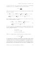


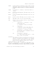

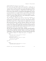


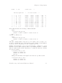


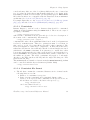


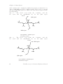
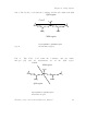
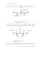


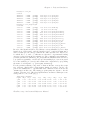
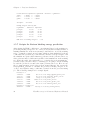


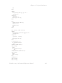


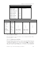


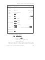


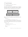


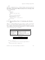


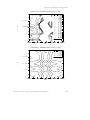
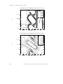

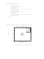
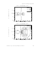
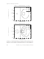


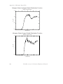
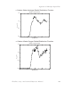
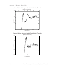

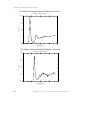
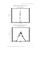
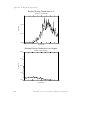
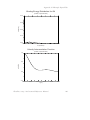


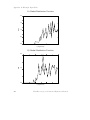
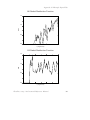


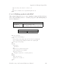

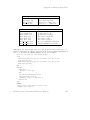

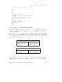


![RUMD User Manual [Version 3.0]](http://vs1.manualzilla.com/store/data/005734566_1-539a984f38202face31c4a646ef91457-150x150.png)