Download Interactive Network Exploration with Orange

JSS
Journal of Statistical Software
April 2013, Volume 53, Issue 6.
http://www.jstatsoft.org/
Interactive Network Exploration with Orange
Miha Štajdohar
Janez Demšar
University of Ljubljana
University of Ljubljana
Abstract
Network analysis is one of the most widely used techniques in many areas of modern science. Most existing tools for that purpose are limited to drawing networks and
computing their basic general characteristics. The user is not able to interactively and
graphically manipulate the networks, select and explore subgraphs using other statistical
and data mining techniques, add and plot various other data within the graph, and so on.
In this paper we present a tool that addresses these challenges, an add-on for exploration
of networks within the general component-based environment Orange.
Keywords: networks, visualization, data mining, Python.
1. Introduction
Network analysis is one of the most omnipresent approaches in modern science, with its
use ranging from social sciences to computer technology to biology and medicine. Tools
for graph drawing and computing their characteristics are readily available, either for free
(Gephi, Bastian, Heymann, and Jacomy 2009, Graphviz, Ellson, Gansner, Koutsofios, North,
and Woodhull 2001, Network Workbench, NWB Team 2006, NetworkX, Hagberg, Schult,
and Swart 2006, Pajek, Batagelj and Mrvar 1998) or in commercial packages (e.g., NetMiner,
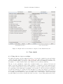
Cyram 2003). An overview of such tools and their capabilities is provided in Table 1.
Most graph visualization and analysis tools provide a picture about the system behind the
graph as whole (e.g., Pajek, igraph, Csardi and Nepusz 2006, and statnet, Handcock, Hunter,
Butts, Goodreau, and Morris 2008). Pajek is a package for the analysis of large networks,
while statnet’s specific focus is simulation of exponential random graph models and statistical
analysis. Much less effort has been put into making the graph analysis software interactive,
by allowing local exploration of the graph, testing how the graph structure depends upon its
construction parameters, letting the user extract data from subgraphs and use it for further
analysis, and so on.
2
Interactive Network Exploration with Orange
Open source
Pajek
NetMiner
NetworkX
Graphviz
igraph
statnet
Gephi
Network Workbench
Net Explorer
Interactive UI
Scripting interface (in Python)
×
×
×
×
×
×
×
×
× (×)
× (×)
× (×)
×
×
×
×
× (×)
Table 1: An overview of the software for network analysis.
For example, edges in most graphs are abstractions of numerical relations. In genetic networks,
two genes are connected, for instance, if they are sufficiently co-expressed. Two journal papers
are related if they share a sufficient number of keywords, and people in a social network can
be connected for having enough shared interests or friends. We would wish for a tool in which
changes in the graph construction parameters (e.g., connection thresholds) can be immediately
observed in the graph itself since sometimes precise tuning is required to get the graph which
reveals interesting relations.
A similar problem is filtering of graph’s nodes. A geneticist might wish to filter out certain
genes, or a computer network expert might want to plot the graph with only the major nodes
or, for another purpose, with every single client. It would be helpful if they were able to
perform such operations interactively, in a script, or both.
Interactive tools are also required to explore the local graph structure itself. Questions like
“Which computers are at most two connections away from those infected?” are asked more
often than “How well do the degrees of the graph’s nodes match the power law?”.
Finally, exploration of the graph often leaves us with a subgraph, or a subset of nodes that we
want to explore further. After identifying a strongly connected component of a social network,
we might want to learn about how this group differs from the general population. If we find a
set of drugs with similar effects on the organism, we might want to discover what is typical of
their active parts. Such questions can be answered with less effort if the network visualization
tool is integrated into a larger statistical, machine learning, or data mining framework.
This paper presents our approach to those problems, a collection of widgets and Python
modules for interactive network visualization and analysis for the data mining toolbox Orange (Demsar, Zupan, and Leban 2004). There are some excellent Python packages for network
analysis (e.g., PyGraphviz, a Python package that interacts with the Graphviz program to
create network plots from the NetworkX graph objects). However, Orange Network add-on
is – to our knowledge – the only Python software for interactive network visualization and
exploration.
The following section briefly introduces the Orange framework as much as necessary for understanding the context of the new add-on, which is presented in more detail in the third
section. The largest section of the paper is dedicated to several use case demonstrations.
Journal of Statistical Software
3
2. Orange and Orange Canvas
Orange is an open source Python library for machine learning and data mining. The library
includes a selection of popular machine learning methods as well as many various preprocessing methods (filtering, imputation, categorization. . . ), sampling techniques (bootstrap,
cross-validation. . . ), and related methods.
Python is a popular modern scripting language, featuring clean syntax, powerful but nonobtrusive object oriented model, built-in high level data structures, complete run-time introspection, and elements of functional programming. It ships with a comprehensive library of
routines for string processing, system utilities, internet-related protocols, data compression,
and many others. These can be complemented by freely available libraries like SciPy (Jones,
Oliphant, and Peterson 2001), which includes a library for matrix manipulation and linear
algebra Numpy (Ascher, Dubois, Hinsen, Hugunin, and Oliphant 2001), the statistical library
stats, and many other scientific libraries.
Similar to R (R Core Team 2013) where some libraries are written in low level languages
(Fortran, C) and others in R itself, the fast core of Orange is written in C++ and other
modules are written in Python.
The code below shows how to use the Orange library from Python. In this paper we will
mostly use the machine learning terminology related to modeling. In classification problems,
we are given labelled data; each data instance belongs to a certain class. It loads Fisher’s Iris
data set, and selects data instances from classes versicolor and virginica. Then it randomly
splits the data into two subsets for fitting the model and for testing it, train and test.
Next we run a learning algorithm. Machine learning makes a distinction between a learning
algorithm (or learner) and classification algorithm (classifier). The latter is a predictive model
for discrete outcomes and the former is an algorithm for fitting the model to the (training)
data. In the code below, the learning algorithm for logistic regression (LogRegLearner) gets
the data as input and returns a classifier (variable logreg). Classifier is an algorithm that
gets a data instance and predicts its class. In the loop at the end of the code, we count the
number of class predictions for the test data (test) that match the actual classes. Finally,
the script reports the proportion of correctly classified test instances.
import Orange
data = Orange.data.Table("iris")
data = data.filter(iris=["Iris-versicolor", "Iris-virginica"])
data = data.translate(Orange.data.Domain(data.domain.features, \
Orange.data.preprocess.RemoveUnusedValues(data.domain.class_var, data)))
folds = Orange.data.sample.SubsetIndices2(data, 0.7)
train = data.select(folds, 0)
test = data.select(folds, 1)
lr = Orange.classification.logreg.LogRegLearner(train)
corr = 0.0
for inst in test:
if lr(inst) == inst.get_class():
corr += 1
4
Interactive Network Exploration with Orange
print "Accuracy:", corr / len(test)
To continue the example, we compared the classification accuracy (implemented in module
Orange.evaluation.scoring) of several algorithms (logistic regression with a stepwise variable
selection, pruned classification trees, and k-nearest neighbor model) using cross-validation
sampling technique from module Orange.evaluation.testing.
from Orange.classification import logreg, tree, knn
from Orange.evaluation import scoring, testing
models = [logreg.LogRegLearner(stepwiseLR = True),
tree.TreeLearner(min_instances = 2, m_pruning = 2),
knn.kNNLearner(k = 3)]
res =
cas =
print
print
print
testing.cross_validation(models, data)
scoring.CA(res)
"Logistic regression:", cas[0]
"Classification tree:", cas[1]
"K-nearest neighbor:", cas[2]
Using such scripts is only suitable for experts with enough programming skills and does not
allow for visual exploration and manipulation of the data.
Orange Canvas provides a graphical interface for these functions. Its basic ingredients are
widgets. Each widget performs a basic task, such as reading the data from a file in one of the
supported formats or from a data base, showing the data in tabular form, plotting histograms
and scatter plots, constructing various models and testing them, clustering the data, and so
on.
Widgets can require data for performing their function and can output data as result. The
most common data type are sets of data instances; other types include models, model constructors, and many others. Types are organized into a hierarchy, so a widget may require,
for instance, a general prediction model or a specific one, such as logistic regression.
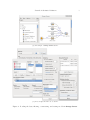
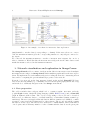
We set the data flow between the widgets by connecting them into a scheme: we put the
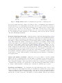
widgets onto the canvas and connect their inputs and outputs. Figure 1(a) shows a scheme
that performs the same procedure as the last code snippet. The File widget reads the data,
Select Data selects instances of versicolor and virginica, and gives them to the Test Learners. The latter also gets learning algorithms from Logistic Regression, Classification
Tree, and k Nearest neighbors, performs the cross validation, and shows the results.
Double clicking the widget brings up a dialog with the widget’s settings and, depending upon
the widget type, its results. Some widgets from the scheme are shown in Figure 1(b).
The power of Orange Canvas is its interactivity. Any change in a single widget – loading
another data set, changing the filter, modifying the logistic regression parameters – instantly
propagates down the scheme (unless the propagation is explicitly disabled, or the change
needs a confirmation by the user).
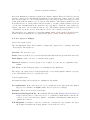
We can add a Scatter Plot widget to the above scheme and give it the filtered Iris data
from Select Data (Figure 2). Then we connect the Test Learners widget to a Confusion
Matrix that shows how many data instances from each class (corresponding to rows) were
Journal of Statistical Software
(a) An example of Orange Canvas scheme.
(b) A few widgets from the above scheme.
Figure 1: Loading the data, filtering, constructing, and testing models in Orange Canvas.
5
6
Interactive Network Exploration with Orange
Figure 2: An example of a scheme for interactive data exploration.
(mis)classified to another class (corresponding to columns). If the user selects one or more
cells, the Confusion Matrix gives the corresponding instances to any widgets connected to
its output.
We connected the Confusion Matrix to another of Scatter Plot’s inputs, the one for a
subset of instances. Wired like this, the Scatter Plot widget shows the entire data set and
marks the instances selected in the Confusion Matrix.
3. Network visualization and exploration in Orange Canvas
The Orange Network add-on consists of widgets and modules for interactive network analysis.
Net Explorer is a widget for Orange Canvas which visualizes graphs and lets the user explore
them. We implemented several auxiliary widgets for reading the network, constructing it from
data, and for computing the general statistical properties of the network.
Network object is stored in the data structure defined in the module NetworkX. We have
added some new algorithms (e.g., community detection and frequent graph pattern discovery)
and methods to seamlessly integrate it into the Orange environment.
3.1. Data preparation
The add-on includes three widgets which load or construct graphs. Net File reads the
popular Pajek format, Graph Modeling Language (GML, Himsolt 1996), and a NetworkX
graph in Python’s pickle format. The objects corresponding to the nodes can be described
with vectors of continuous, discrete, or textual variables (or, in machine learning terminology,
attributes). The user can supply additional data in different formats: tab-delimited, commaseparated, or in several other formats used by other software. The second optional file contains
the data about the edges. The data needs to include two columns marked u and v with indices
of node pairs, and an arbitrary number of other columns with the data about the given pair.
Journal of Statistical Software
7
Net from Distances constructs a graph from a distance matrix. Edges are defined by several
criteria: connect nodes with distances within the specified interval, connect each node with
its k nearest neighbors, or nodes with distances up to the i-th percentile. The widget provides
a histogram with the number of node pairs at each distance. The distance matrix can come
from various sources: a widget that reads it from a file or one that computes distances between
objects. Net from Distances also includes some basic filters: output the entire graph, the
largest component, or nodes with at least one edge. The distance matrix can include vectors
of attributes, about the objects. Such data is copied to the constructed network.
The last widget for construction of networks is SNAP, which downloads the network from the
Stanford Network Analysis Project graph library (http://snap.stanford.edu/data).
3.2. Net Explorer widget
Input and output signals
The Net Explorer widget has a number of input and output slots to exchange data with
other widgets. The inputs are:
Network: The network to plot.
Items: Data about the nodes (overrides any such data that is already present in the network).
Item Subset: A list of nodes to be marked in the graph.
Distances: Distances between graph nodes, required by some layout optimization algorithms.
Net View: A custom plug-in widget for extending the Net Explorer.
The widget can output a selected subgraph and the corresponding distance matrix or descriptions of the marked, selected, or unselected nodes.
Layout optimization
Net Explorer supports several layout optimization algorithms:
No optimization: If the given network object contains the nodes placement data (this is
supported, for instance, in Pajek format), they are placed accordingly.
Random: The nodes are scattered randomly.
Fruchterman-Reingold (F-R): The standard F-R algorithm (Fruchterman and Reingold
1991) positions pairs of connected nodes to a certain fixed small distance and the unconnected ones to the fixed large distance. A simulated annealing algorithm is used to
optimize the solution.
F-R Weighted: A variation of the above that also considers the edge weights: the larger
the weight, the smaller the desired distance between the two nodes.
8
Interactive Network Exploration with Orange
F-R Radial: An F-R-type algorithm which places a node selected by the user at the center
and optimizes the layout around it. The optimization procedure ensures that nodes
with shorter paths to the central node are closer to it than those with longer paths.1
Circular Crossing Reduction: A local optimization algorithm which puts the nodes around
the circle and tries to minimize the number of edge crossings (Baur and Brandes 2004).
Circular Original: Nodes are placed around the circle in the order they are given in the
data.
Circular Random: The nodes are placed around the circle in random order.
FragViz: The FragViz (Stajdohar, Mramor, Zupan, and Demšar 2010) algorithm for visualization of networks that consist of multiple unconnected components. The algorithm
combines the standard Fruchterman-Reingold algorithm for laying out individual components with an MDS-style algorithm for placement and rotation of components.
MDS: The SMACOF (De Leeuw and Mair 2009) multidimensional scaling algorithm using
stress-majorization. The stress model simulates a set of balls corresponding to graph
nodes that are connected by springs. The lengths of the springs correspond to the
desired distances between the graph nodes.
Pivot MDS: An approximation of the classical MDS algorithm, where k pivots (columns)
are randomly selected to reduce the distance matrix size (Brandes 2007).
The latter three algorithms require information on preferred distances between the nodes
provided on a separate input slot. The last two algorithms place nodes according to the
provided distances only, disregarding the network edges.
The user can specify the number of iterations of the optimization procedure where applicable.
The default is set such that the optimization is expected to take approximately five seconds.
With a higher number of iterations, the optimization takes longer but the results are often
considerably better.
In practice, if the number of nodes is large, the most applicable algorithms are FruchtermanReingold algorithms, with the Random placement used to reinitialize the optimization if it
gets stuck in a local minimum. The user can also move individual nodes or groups of selected
nodes after or even during the layout optimization.
Setting visual parameters
The widget allows the user to set a number of parameters (see, for instance, Figure 6(b)). The
widget can print a label with the meta-data beside each node. When the number of nodes
is excessive, the user can reduce the clutter by reducing the number of shown variables, or
by printing out only the data about the node below the mouse pointer. Another option is
to annotate only the marked nodes. It is also possible to print some data at each node, and
display more on the mouse hover over the node.
Nodes can be colored or sized according to values of the corresponding objects’ attributes.
The widths of edges can correspond to their weights, and can be colored according to the
value of the selected attribute from the edge descriptions.
1
The algorithm will be published elsewhere.
Journal of Statistical Software
9
Marking and selecting
The widget uses a two-stage procedure for node selection that allows for a very flexible manipulation of subsets of nodes (see, for instance, Figure 6(a)). Nodes can be marked or selected
or both. Marking is often a pre-stage to selecting or deselecting. Selected nodes are shown by
filled circles (as opposed to the rest which are hollow), whereas marked nodes have a black
border.
Nodes can be selected manually by clicking or by drawing selection rectangles. Another way
to select nodes is to add or remove the marked nodes to or from the selection, or to replace
the current selection with the marked nodes. The selected nodes can be moved to manually
enhance the layout. The user can also hide the selected or the unselected nodes, and then
rerun the optimization. The selected subgraph, the data or distance sub-matrix about the
corresponding objects can also be fed on to other widgets.
The nodes can be marked upon values of attributes of the corresponding objects or upon
network properties. To select local portions of the graph, the user can mark the neighbors of
a node pointed to by the mouse, or the neighbors of the selected nodes up to a certain distance
(e.g., up to three edges away). Hubs, poorly connected nodes, and similar local phenomena
can be observed by marking the given number of the most connected nodes, the nodes with
more or less edges than given number, or with more connections than their average neighbor
or than any of its neighbors. Finally, the set of marked nodes can be specified by the data
sent from another widget using the input slot Item Subset.
Plug-ins
A network plug-in is a widget that controls which part (subgraph) of the original network
is visualized in the Net Explorer. It is particularly useful for visualizing large networks. A
plug-in widget connects to the Net Explorer’s “Net View” signal.
Net Inside View widget is an example of a basic plug-in. It provides a local view on the
network. On selection, it smoothly moves selected node to the center, and hides distant
nodes (nodes that are more than k edges away). An expert can then interactively explore the
network by clicking on neighboring nodes.
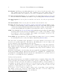
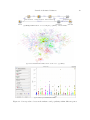
Pubmed Network View is a plug-in that provides a view on the large Pubmed article network. The user can first filter the articles and then select a set to display. In addition to
selected articles, neighboring articles are also included if they satisfy selection criteria (edge
distance from selected, maximum number of neighbors, and edge threshold). Right-clicking
the article in the Net Explorer pops-up a menu of options: to remove, expand, or score the
corresponding article. In the example in Figure 3 the article “Detecting protein function and
protein-protein interactions from genome sequences” was selected and displayed together with
the most similar articles (at most 2 edges away and with edge weight higher than 0.5).
3.3. Network analysis
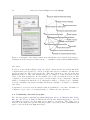
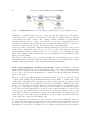
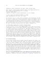
The Net Analysis widget computes graph- and node-level statistics for the given network.
Graph-level indices are computed and displayed in the widget (Figure 4(a)). These include
the number of nodes and edges, average node degree, graph diameter, average shortest path
length, density, degree assortativity coefficient, graph clique number, graph transitivity, average clustering coefficient, number of connected components, number of attracting components,
10
Interactive Network Exploration with Orange
Figure 3: A subgraph of the Pubmed article network with the selected article “Detecting protein function and protein-protein interactions. . . ,” visualized together with 14 similar articles.
and others.
For the node-level indices (Figure 4(b)), the widget outputs another network in which the
computed indices are appended to each node in the same way as, for instance, the Net File
widget appends the data read from the file. This data can then be explored in the Net
Explorer widget or other data analysis widgets, for example to build a prediction model
based on the network structure. For an example, refer to the case study in Section 4.3. The
computed node level indices are node degree, average neighbor degree, clustering coefficient,
number of triangles in which the node participates, number of cliques, degree centrality,
closeness centrality, betweenness centrality, information centrality, core number, eccentricity,
and others.
Computation of selected network analytic tasks is parallelized to save time. In multi-core
computers, one processor core is always left free to enhance the user experience.
3.4. Community detection in graphs
Two label propagation clustering algorithms (Raghavan, Albert, and Kumara 2007; Leung,
Hui, Liò, and Crowcroft 2009) are implemented in the Net Clustering widget. As both
algorithms are iterative, the user must set the number of iterations. The widget gets a
network on the input, and appends clustering results to the network data. Communities can
then be explored in the Net Explorer widget.
Journal of Statistical Software
(a) graph-level indices
11
(b) node-level indices
Figure 4: Graph- and node-level indices computed on the Last.fm network.
4. Case study
4.1. Using the Net Explorer widget
We shall demonstrate the Net Explorer widget on a network of musical groups and artists
obtained from the Last.fm web radio http://last.fm/. The website provides a list of the
five most similar artists or groups for each given artist, where the similarity is measured by
the number of common listeners (the exact definition is not publicly available).
The site does not publish the complete list of available artists, so we constructed the network
using a search algorithm that started with a small set of artists from diverse musical styles
(U2, Johann Sebastian Bach, Norah Jones, Erik Satie, and Spice Girls), and then expanding
it by querying for the artists who are similar to those in the set. We stopped the search after
several days, when the set contained around 320, 000 nodes. After removing those for which we
did not query for similar artists, we got a set with around 26, 000 artists. We further reduced
it by taking only the 2000 most connected artists. We took the largest connected subgraph
(popular music), and retrieved additional data about the corresponding artists and groups:
12
Interactive Network Exploration with Orange
Figure 5: Orange Canvas scheme for showing the graph and the corresponding meta data.
the number of albums released, the year of their first and last album release, the number
of times they have been played on Last.fm and the number of distinct listeners, and lists
of user-assigned tags (like “country,” “60s,” “female vocalists,” “Russian rock,” and similar).
Last.fm weights the tags according to how well they correspond to a particular artist. For
each artist, we identified the tag with the greatest weight and assumed that it corresponds to
the genre to which the artist belongs. The data was retrieved in March 2007.
Since some of these data (album count, first and last album release year) were retrieved from
another service, AOL music http://music.aol.com/, we removed the artists for which the
queries returned ambiguous results, mostly due to more than one group having the same
name. The resulting graph contains 1262 nodes representing the most established popular
music groups and artists.
The purpose of this study is not to provide new insights into the Last.fm data but to merely
demonstrate the use of the Net Explorer widget. An interested reader will find the detailed
analysis of this network in the works of Celma (2010) and Nepssz (2009).
Basic graph manipulation, marking and selecting. Scheme from Figure 5 loads the
graph and additional data about nodes (Net File widget). The data is shown in the Data
Table, and the graph is plotted in the Net Explorer widget. To observe the subgraphs that
we are going to select in the Net Explorer, we attached another Net Explorer and Data
Table to its output.
When we open the Net Explorer and select variable “artist” for the node labels, the graph
– despite being optimized by the Fruchterman-Reingold’s algorithm – looks like a huge cloud
of unreadable overlapping labels. Say that we are interested in exploring the vicinity of Paul
Simon. In the Mark tab we select Find nodes and type “Paul Simon.” This finds and marks
the node corresponding to Paul Simon (the node is drawn as a filled circle with black border,
as opposed to others that are empty). We can then click the button for selecting the marked
nodes. This selects the Paul Simon’s node (the node is now filled but has no border). We can
proceed by choosing “Mark neighbors of selected nodes”, and set the distance to, say, 2. This
marks all nodes that are at most three connections from Paul Simon. To further reduce the
visual clutter, we check “Show labels on marked nodes only”, and zoom in the marked part
of the graph. The result is shown in Figure 6(a).
We can again select the marked nodes, and output the corresponding subgraph. Since the
second Net Explorer shows only the subgraph, the resulting layout is much nicer as it is
not affected by other artists in which we are not interested at the moment. We added the
information about genres by coloring the nodes according to the tag that best describes them,
Journal of Statistical Software
(a) Vicinity of Paul Simon in the entire graph.
(b) Subgraph with additional data visualization; the number of plays as size and genre as color.
Figure 6: Exploration of artists similar to Paul Simon.
13
14
Interactive Network Exploration with Orange
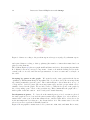
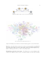
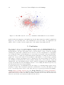
Figure 7: Genres according to the prevalent tag in each region, as judged by a human expert.
and resized them according to their popularity (the number of times their music has been
played) on the Last.fm.
The result in Figure 6(b) shows a graph with Paul Simon and a few other artists (in particular
Bob Dylan) between two stronger components – classic rock with the Rolling Stones as the
central point on one side, and various representatives of a more acoustic and vocal style on
the other.
Grouping by genres in the graph. We again drew the entire graph with the layout
optimized by Fruchterman-Reingold algorithm, and colored all nodes by the most important
tag, which presumably gives the genre. The result in Figure 7 shows that there is a good
correspondence between genres (the most important tags), and the groups which can be
visually observed in the graph. We are indeed able to easily label regions of the graph by
the corresponding “genre” based on the prevalent tag. This confirms that the graph can be –
with a grain of salt and caution – used for subjective visual clustering.
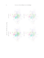
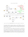
Development of genres. To observe how the musical genres evolved over time we plotted
the same graph as before, but used the Select Data widget (Figure 8) to select subsets of
artists based on the year of their first album release, and used this data to select the nodes
in the Net Explorer by feeding it to the “Items Subset” slot. The artists active before the
selected year were represented with filled symbols.
Figure 9 shows graphs for artists active before years 1985, 1990, 1995, and 2000. Before 1985,
Journal of Statistical Software
15
Figure 8: Orange Canvas scheme for analysing the appearance of musical genres.
most active artists performed “classic rock” (this probably covers multiple genres which most
Last.fm’s listeners do not distinguish between). We can notice some soul, hard rock and pop
groups, and of course, the 80’s tag. In the next image (before 1990) even more groups in these
genres are active. We also see the emergence of funk music. By 1995 most of the popular
groups from these genres are present, and there are a lot of new genres, such as metal, hip
hop, rap, R&B, indie, punk, and hardcore. The last image adds electronic and emo, and the
only style still missing is minimal.
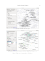
K-means clustering in the graph. Using the widget for k-means clustering (Figure 10(a)),
we split the musicians into 22 clusters. The distance was defined as the Manhattan distance
between the weights of tags (tags not appearing at a certain artist were assigned a weight of 0).
The number of clusters was determined by the Bayesian information criterion (BIC) (Schwarz
1978). BIC estimates the quality of clustering as a combination of log-likelihood and a penalty
term for the number of free parameters, which includes the number of clusters. We colored
the nodes corresponding to their respective clusters (Figure 10(b)), and found a good correspondence between the apparent “graph clusters” and k-means clustering. This can be the
result of using the tags (the basis for the clustering) in the definition of similarities (the basis
for the graph) as reported by the Last.fm. However, since the available documentation on
the Last.fm states that the definition is mostly based on the number of common listeners, the
most plausible explanation is that a typical listener sticks to a certain kind of music denoted
by the same set of tags. This can thus be an informal practical verification of reliability of
the tagging system.
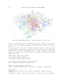
Genres and number of albums. Sizing the nodes by the number of released albums
(Figure 11) gives a rough impression about the number of albums per genre and its variation.
The picture suggests that artists from some genres generally release much more albums than
their colleagues belonging to other genres. However, there is a correlation between the number
of albums released and the year of publication of the first album (Spearman rank correlation
is −0.70), so different number of albums can be attributed to different ages of genres.
Popularity and influence. To demonstrate how the graph widget can be used to select
data, we first plotted the artists in a scatter plot in which we separated the groups by their
clusters by using the cluster ID (genre) for the x axis, and the y axis represents the number
of times the artist was played on Last.Fm (Figure 12). The colors represent different clusters,
and the size of points correspond to the number of released albums. Then we used the Net
Interactive Network Exploration with Orange
16
(c) before 1995
(a) before 1985
(d) before 2000
(b) before 1990
Figure 9: Genre appearance by periods.
Journal of Statistical Software
17
(a) The Net Explorer widget connected to the k-means clustering.
(b) Nodes in the same cluster share the same color.
Figure 10: Finding network clusters by k-means clustering applied on network meta-data.
Explorer to select the 50 most connected nodes; these nodes represent the most influential
artists. We fed these hubs to the Scatter Plot widget, which marked them by filling the corresponding symbols. With only 50 out of 1262 artists selected, we see that a disproportionate
number of them appears at the top of their corresponding clusters.
Manipulating graph data from scripts. We will show how to use the Python module
behind the Net Explorer widget directly, by scripting in Python. We will verify the finding
18
Interactive Network Exploration with Orange
Figure 11: Graph with the number of albums represented by the node size.
from the previous example, namely, that influential groups (those with more connections) are
also among the most popular groups (that is, the most listened to) within their respective
genres.
To exclude the effect of the genre, we divided the number of plays for each artist by the
maximum number of plays in the corresponding genre (genres were defined by the k-means
clustering). We then used the Mann-Whitney test to compare the number of plays for the
group of the 50 most connected artists with the other artists. The difference was highly
significant (p < 0.01).
import numpy, scipy.stats, Orange
from operator import itemgetter
from Orange.clustering import kmeans
net = Orange.network.readwrite.read("lastfm.net")
data = Orange.data.Table("lastfm_tags.tab")
manhattan = Orange.distance.Manhattan
kmeans = kmeans.Clustering(data, centroids = 22, distance
=manhattan)
plays_clust = \
[(row["plays"], clust) for (row, clust) in zip(data, kmeans.clusters)]
maxs = \
[max(plys for (plys, clust) in plays_clust if clust==c) for c in range(22)]
Journal of Statistical Software
(a) Orange Canvas scheme for observing the popularity of network hubs.
(b) Network with marked hubs and node size set to popularity.
(c) A scatter plot with marked hubs.
Figure 12: Correspondence between the influence and popularity within different genres.
19
20
Interactive Network Exploration with Orange
normalized = [plys / maxs[clust] for (plys, clust) in plays_clust]
hubs, degrees = zip(*sorted(net.degree().items(), key=itemgetter(1))[-50:])
hubp = numpy.array([normalized[i] for i in hubs])
not_hubp = numpy.array(
[plys for (i, plys) in enumerate(normalized) if i not in hubs])
u, prob = scipy.stats.mannwhitneyu(hubp, not_hubp)
print "Mann-Whitney U: %d, p=%e" % (u, prob)
Note that this is only a toy example. The experimental procedure is invalid since the same
data is used to formulate and to validate the hypothesis. Besides, if the similarity between
two artists depends upon the number of mutual fans not normalized by the number of fans of
each individual artists, the artists which are more popular get more connections simply due to
their popularity, and the discovered relation follows directly from the definition of similarity.
We cannot verify this since Last.fm keeps the exact definition of similarity secret.
4.2. Extending existing data analysis in Orange Canvas
Net Explorer widget can extend existing Orange Canvas schemes, which often yields additional insights about the problem domain. Consider the example in Figure 1, where the aim
is to build a prediction model on the Iris data set. Although the classification accuracy of
the k-nearest neighbor classifier is high (0.94), we wish to further explore the instances where
the model fails. We connect the Select Data with the Example Distance widget, add the
Net from Distances and Net Explorer widgets as in Figure 13(a), and select misclassified
instances of the k-nearest neighbors model in the Confusion Matrix widget. In the Net
from Distances widget we connect each node with the 3 most similar nodes, to simulate the
behavior of the k Nearest Neighbors widget’s model exactly. After observing the outliers
in Net Explorer (Figure 13(b)), and toying with different distance measures, we notice that
it is not possible to further increase the classification accuracy without overfitting the data.
4.3. Network mining
Network widgets seamlessly integrate machine learning algorithms into the analysis of network data. The air traffic network in this example was constructed by parsing timetables
of three major airlines: Lufthansa, United, and American Airlines. Graph nodes represent
airports; a pair of nodes is connected if any of the listed airlines provides a direct flight between them. Airport data was extracted from the World Airport Traffic Report issued by
the Airport Council International in 2006. The network data set includes: number of aircraft
movements (landing or take-off of an aircraft), number of passengers arriving or departing
via commercial aircraft, cargo handled in tonnes, airport category as specified by the Federal
Aviation Administration (Large Hub, Medium Hub, Small Hub, Nonhub Primary, and Nonprimary Commercial Service), and a class variable “FAA Hub” specifying whether the airport
is considered a hub by the FAA or not.
Figure 14 shows the Orange Canvas scheme of the analysis. On the first glance, there are
two major communities of airports. We confirmed this with the Net Clustering widget:
applying the community detection method by Raghavan et al. (2007) and coloring the nodes
Journal of Statistical Software
(a) Orange Canvas scheme (extended from Figure 1).
21
(b) The 3-nearest neighbor network;
misclassified instances are marked.
Figure 13: Analysis of misclassified examples on Iris data using the Net Explorer widget.
Figure 14: The complete Orange Canvas scheme used in the analysis of air traffic data.
by the clustering result indeed revealed two clusters. See results in Figure 15 where colors
represent the two discovered communities. We then set the node tooltips to show the attribute
“city”, and hovered over some airports from each cluster. We discovered that the airports are
clustered according to the continents, and the two large communities represent airports in
the North America and Europe.
Our next objective was to explore the correlation between the network topology and the airport type, more specifically, to predict weather the airport is a hub or not from the network
topology. First, 14 node-level indices were computed with the Net Analysis widget (Figure 4(b)). They were scored and compared in the Rank widget. The top half of the ranked
attributes (according to the ReliefF measure of Kononenko (1994)) were used to test different learning algorithms (logistic regression, naive Bayes, random forest, and support vector
machines). Examples that were misclassified by the logistic regression learner (the model
with the best classification accuracy, 0.73) were selected in the Confusion Matrix widget,
22
Interactive Network Exploration with Orange
Figure 15: Air traffic network colored by communities. Misclassified nodes are marked.
marked in the Net Explorer, and finally, listed in the Data Table (see marked examples in
Figure 15). It seems that most of the classification errors were made on peripheral nodes
which could be a result of the incompleteness of the analysed air traffic network.
5. Conclusion
We presented a new tool for visual analysis of network data – the Orange Network add-on.
Many similar tools exist, though ours differs in offering a very interactive and flexible, yet user
friendly interface. We have demonstrated how to use the widget for basic operations on graphs
(drawing the graph with optimized layout, selection of nodes, magnification of subgraphs,
etc.). Using the widget for data filtering, we observed the development of the network in time.
We showed how to combine the graph with k-means clustering to identify the clusters in the
graph. We observed the relation between influence (the number of connections), popularity
(the number of plays), and musical genre by filtering the data and plotting it in the scatter
plot. Finally we demonstrated how a more advanced study can be done by the use of network
analysis and other data mining widgets. Beside visual programming in the Orange Canvas,
we have shown that the network analysis can also be done calling the functions provided by
the library directly from a script in Python.
Powerful exploratory tools naturally increase the danger of conducting inappropriate experimental procedures. The researcher’s awareness of what such tools can do and what not, and
how to test the hypotheses based on the data, is however a general problem in data mining.
Orange (http://orange.biolab.si/), the Orange Network add-on (http://bitbucket.
org/biolab/orange-network/), and all required third party libraries are available under the
GNU GPL license for Microsoft Windows, Linux, and Mac OS X. Networks and data sets
that were used in the case study are included in the add-on.
Journal of Statistical Software
23
Acknowledgments
We would like to thank the members of Bioinformatics Laboratory at the Faculty of Computer
and Information Science, Ljubljana, Slovenia, for their suggestions during development of the
add-on, and in particular, to Lan Umek for his help in finding a suitable testing procedure
for the first case study.
References
Ascher D, Dubois PF, Hinsen K, Hugunin J, Oliphant T (2001). Numerical Python. URL
http://www.numpy.org/.
Bastian M, Heymann S, Jacomy M (2009). “Gephi: An Open Source Software for Exploring
and Manipulating Networks.” In International AAAI Conference on Weblogs and Social
Media. URL http://gephi.org/.
Batagelj A, Mrvar V (1998). “Pajek – Program for Large Network Analysis.” Connections,
21, 47–57. URL http://pajek.imfm.si/.
Baur M, Brandes U (2004). “Crossing Reduction in Circular Layouts.” In Proceedings of the
Workshop on Graph-Theoretic Concepts in Computer Science, WG 2004, pp. 332–343.
Brandes U (2007). “Eigensolver Methods for Progressive Multidimensional Scaling of Large
Data.” In M Kaufmann, D Wagner (eds.), Graph Drawing, volume 4372 of Lecture Notes
in Computer Science, pp. 42–53. Springer-Verlag, Berlin.
Celma O (2010). Music Recommendation and Discovery. Springer-Verlag.
Csardi G, Nepusz T (2006). “The igraph Software Package for Complex Network Research.”
InterJournal, Complex Systems, 1695.
Cyram (2003). NetMiner User Manual. Seoul. URL http://www.NetMiner.com/.
De Leeuw J, Mair P (2009). “Multidimensional Scaling Using Majorization: SMACOF in R.”
Journal of Statistical Software, 31(3), 1–30. URL http://www.jstatsoft.org/v31/i03/.
Demsar J, Zupan B, Leban G (2004). “Orange: From Experimental Machine Learning to
Interactive Data Mining.” Faculty of Computer and Information Science, University of
Ljubljana. URL http://orange.biolab.si/.
Ellson J, Gansner ER, Koutsofios E, North SC, Woodhull G (2001). “Graphviz – Open Source
Graph Drawing Tools.” Graph Drawing, pp. 483–484. URL http://www.Graphviz.org/.
Fruchterman TMJ, Reingold EM (1991). “Graph Drawing by Force-Directed Placement.”
Software – Practice and Experience, 21(11), 1129–1164.
Hagberg A, Schult D, Swart P (2006). “NetworkX – High Productivity Software for Complex
Networks.” URL http://networkx.lanl.gov/.
24
Interactive Network Exploration with Orange
Handcock MS, Hunter DR, Butts CT, Goodreau SM, Morris M (2008). “statnet: Software
Tools for the Representation, Visualization, Analysis and Simulation of Network Data.”
Journal of Statistical Software, 24(1), 1–11. URL http://www.jstatsoft.org/v24/i01/.
Himsolt M (1996). “GML: A Portable Graph File Format.”
Jones E, Oliphant T, Peterson P (2001). “SciPy: Open Source Scientific Tools for Python.”
URL http://www.scipy.org/.
Kononenko I (1994). “Estimating Attributes: Analysis and Extensions of Relief.” In
F Bergadano, LD Raedt (eds.), Proceedings of the European Conference on Machine Learning (ECML-94), pp. 171–182. Springer-Verlag.
Leung I, Hui P, Liò P, Crowcroft J (2009). “Towards Real-Time Community Detection in
Large Networks.” Physical Review E, 79(6), 1–10.
Nepssz T (2009). “Reconstructing the Structure of the World-Wide Music Scene with Last.fm.”
URL http://sixdegrees.hu/last.fm.
NWB Team (2006). Network Workbench Tool. Indiana University, Northeastern University,
and University of Michigan. URL http://nwb.slis.indiana.edu/.
Raghavan U, Albert R, Kumara S (2007). “Near Linear Time Algorithm to Detect Community
Structures in Large-Scale Networks.” Physical Review E, 76(3).
R Core Team (2013). R: A Language and Environment for Statistical Computing. R Foundation for Statistical Computing, Vienna, Austria. URL http://www.R-project.org/.
Schwarz G (1978). “Estimating the Dimension of a Model.” The Annals of Statistics, 6(2),
461–464.
Stajdohar M, Mramor M, Zupan B, Demšar J (2010). “FragViz: Visualization of Fragmented
Networks.” BMC Bioinformatics, 11, 475.
Affiliation:
Miha Štajdohar
Bioinformatics Laboratory
Faculty of Computer and Information Science
University of Ljubljana
Tržaška 25, Slovenia
E-mail: [email protected]
URL: http://www.fri.uni-lj.si/mihas/
Journal of Statistical Software
published by the American Statistical Association
Volume 53, Issue 6
April 2013
http://www.jstatsoft.org/
http://www.amstat.org/
Submitted: 2009-01-06
Accepted: 2012-11-16