Download PDF

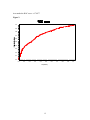
corresponding threshold c varies from ∞ to − ∞ . [13] It has been shown that the area
under a ROC curve equals the unconditional probability of correct ordering, [14] that is
∫ ROC (t)dt = P( y D > y D ) .
Regression models can evaluate the impact of covariates on the accuracy of a
diagnosis test or a bio-marker. When a test or bio-marker is continuous with normal
error, it can be modeled through the standard linear regression model:
y = µ + ε = Xβ + ε
where µ = E( y) is the mean of y and β are the regression coefficients is X . Very
often, these continuous outcomes can be dichotomized by choosing some meaningful
critical value c and defining the test result or bio-marker as positive if it is greater than
the critical value of c. After this conversion, the problem is translated to model the
impact of covariates on binary outcome measures, such as diseased(positive) versus
non-diseased(negative). To model binary outcome measures, one can model functions
of µ rather than µ itself; that is to use generalized linear model (GLM) framework. The
basic form of GLM can be written as η = g ( µ) = Xβ , where η is a link function that
links E ( y) with the linear predictor Xβ . To evaluate the impact of covariates on ROC
curves, one can either model the impact of covariates on a diagnosis test or a biomarker, directly on ROC curve or even on the summary statistics of ROC curve, such
as the area under a ROC curve.
3. Estimating ROC Curve under Repeated Measures Design
Under repeated measures design, each patient will have multiple data points over
time or under different conditions. The observations within a given patient will no
longer be independent and the intra-patient correlation and variation are introduced in
the analyses. Due to intra-patient variation, the impact of covariates on the accuracy of
a diagnostic test or a bio-marker will consist of both fixed global effect (e.g., patient’s
gender) as well as individual patient random effect (e.g., change over time). For both
continuous and non-continuous repeated measure outcome variables, the random
effects from individual subjects can be incorporated in a model through the extension of
GLM to generalized linear mixed model (GLMM),[15] in which the linear predictor
consists of two parts of fixed and random effects.
Let µi = E ( yi | γ i ) be the conditional mean of an outcome variable yi , and let
ηi = g ( µi ) be the link function that connects µi with a linear predictor. Then GLMM
can be written as:
ηi = X i β + Z i γ i
for i=1,…,n.
and the conditional variance is:
Var ( y i | γ i ) = R ,
where yi is a ni x1 vector of test results for the ith patient, ni is the number of outcome
measures for the ith patient, X is n x p containing known covariates that are associated
with the fixed effects. β , the fixed effect parameter vector is px1, and Z i is n i x k
representing known covariates that are associated with the random part of the model.
γ i , the random effect parameter vector is kx1 , is distributed as N (0, G i ) . The
i
i
3