Download The Basics

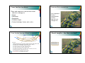
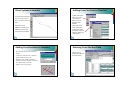
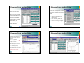
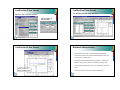
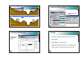
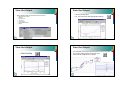
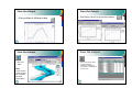
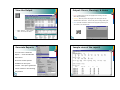
The Basics
HECRAS Basis Input
Geometry Data.
Flow Data.
Perform Hydraulic Computations
by G. Parodi
WRS – ITC – The Netherlands
Viewing the Output
ITC Faculty of Geo-Information Science and Earth Observation of the University of Twente
Before you start…
Layout the model
Extent of study area
Area of interest
Boundary conditions
Section locations and
orientation
Geometry Data - the basics
Cross-section information
Roughness coefficients
Distance between sections
Bridge/culvert data
1
Cross Section Locations
Cross section orientation
Place and measure cross sections when
there is a change in:
Slope
Discharge
Roughness
Channel shape
Control (bridge, levee, weir, etc)
Very important
Survey
perpendicular
to flow
May not be a
straight line
⊥ to flow
Cross Section Spacing: Where to measure?
X1
In
Reach Lengths - Are they constant?
X2
general:
Widely spaced for flat, very large rivers and closer for steep small streams
Very large rivers (Mississippi) on the order of a mile (1600 m)
For large rivers on the order of 1000 feet (300 m)
For slower streams on the order of 200 feet (60 m)
For small creeks on the order of 25 feet (8 m)
For supercritical reaches, on the order of 10 to 50 feet (3 to 15 m)
For drop structures, as low as 5 feet (1 m)
Can interpolate if reasonable (check results)
Not too close (1’, may drop friction loses)
High flow
Low flows
⊥ to flow
2
Survey
Bridge Surveys
Survey shots must describe the channel and overbank flow
•Profile road and bridge deck
centerline
area
•Pier width, location
Section should extend across the entire floodplain
•Low Chord Elevation
Plot cross-section data, especially electronic surveys
•Skew Angle (bridge - stream)
Take photographs
•Bridge opening
Assume modeler has never seen the stream
Note vegetation changes in cross-section e.g. field, trees,
grass buffer, etc.
No 3-point cross-sections
HEC-RAS 3.0 Hydraulic User Manual, Figure 5.1
Starting HEC-RAS
Basic Input - the model
Double Click on HECRAS icon.
ITC Faculty of Geo-Information Science and Earth Observation of the University of Twente
3
Starting a Project
Starting a Project
Select a working directory
Then enter project title and file name
Establish the Unit first
Click on File - New Project
from the main menu to start
a project
Starting a Project
Stream Geometry Data
To add data, click on Edit and
Geometric Data
Check the unit system before accepting.
Units can be change before or after the model is
created.
Or, you can click on
the Geometry Editor
button:
4
Stream Geometry Data
Suggested order of data entry:
River System Schematic
Must be added before any other features.
Draw and connect the reaches of the stream system.
Add River Reach(es) along with any Junctions
(actually, this must be first).
Add Cross-Section names, elevation-station data, ‘n’
values, bank stations, reach lengths, loss coefficients,
etc.
Add Road/Bridge/Culvert and/or Weir/Spillway data.
Draw from upstream to downstream, which will coincide with a flow
direction arrow - generally from top of screen to bottom. Double
click on last point to end.
Connection of 3 reaches is a junction.
Can model from single reach to complicated networks. The river can
even split apart and then come back together.
Can accentuate by adding background bitmap.
River System Schematic
River System Schematic
To add a River Reach, select
the River Reach button from
the Cross-Section Editor
Window.
Then add line(s) representing
the schematic of the river(s)
you are modeling. Single click
between each segment of the
line. After your last line
segment, double click to end.
A window then
pops up to allow
you to enter the:
River name
Reach name
5
River System Schematic
Adding Cross Sections to Reaches
To add cross-section
data, click on the
“Cross-Section”
button from the
Geometry Data
Window.
The program then displays
the river and its name in
blue. The reach name is in
black.
Tributaries and/or
This brings up the
Cross Section Data
window from where
you choose “Options”
and then “Add a new
Cross-Section…”
additional reaches can be
added to the main reach
using the same procedure.
Adding Cross Sections to Reaches
Entering Cross Section Data
Enter the cross-section name (it must be a
You can enter a
lengthy description of
the cross-section.
number
It must be in numerical order - upstream =
highest number) and select OK.
Numbering is not related to progressive.
To add a cross section between two existing
ones, add a number in between.
Number can be real or integers.
3
2
1
6
Entering Cross Section Data
Entering Cross Section Data
There are several options available
This is the main Cross-
to further refine the cross section
Section Data window.
data.
Here you enter the basic
File editing tools
cross-section data such as
Geometric transformations and
rescaling tools
elevation-station data,
Editor of blocking, no flow and
reach lengths, ‘n’ values,
disturbances
bank stations, and
Editors and rescaling of roughness
contraction and expansion
loss coefficients.
Note help note
Note: Orientation is looking downstream
Entering Cross Section Data
A quick visual check of the data is
available through the “Plot Cross
Section (in separate window)“
option.
In ‘x’ the progressive
In ‘y’ the absolute elevation with
respect to a datum
Dots show stations
Red dots separate channel from
banks (left and right)
‘n’ values display on top
Coordinates display as the mouse
is moved around.
ORIENTATION IS LOOKING
DOWNSTREAM!!
Entering Cross Section Data
XSections can be plotted from the editor.
7
Entering Cross Section Data
Notes on Cross-Section Data
Other but present sections can be shown in the same plot.
Ideal to check relative shape and elevation differences.
X-sections should extend across the entire floodplain and be perpendicular to
anticipated flow lines (approximately perpendicular to ground contour lines).
X-sections should accurately represent stream and floodplain geometry. Put in
where changes occur in discharge, slope, shape, roughness, and bridges.
Enter X-Section elevation-station data from left to right as seen when looking
downstream.
Cross-Sections should start far enough downstream to “zero out” any errors in
boundary conditions assumptions (for sub-critical profile). Far from upstream for
super-critical flow. The section of analysis should be farm from boundary errors.
Study Area
Actual Profile
Uncertain WS
Notes on Cross-Section Data (cont)
Location of X-sections within a reach varies with the intensity of the study and
the conditions of the reach
Higher number X-section river stations are assumed to be upstream of lower
number river stations. Slope areas require more X-sections.
The left and right channel banks, must be given at a station located in the Xsection elevation-station data set. (Figure shows only right bank)
The choice of friction loss equations will also affect X-section spacing and
predicted flood elevations
Notes on Cross-Section Data (cont.)
The left side of the X-section, looking downstream, is assumed to have the lower
X values and progress right as the X values increase, (can not narrow the section)
Boundaries are fixed, can not reflect changes during a storm (scour deposition).
X-section endpoints that are below the computed water surface profile will be
extended vertically to contain the routed flows with area/wetted perimeter
reflecting this boundary condition. To avoid this, be certain that the cross section
extends till a place where flood does not occur.
X original right bank endpoint
Vertical extension of the section
endpoint if the water floods it
Better right bank endpoint
8
Notes on Cross-Section Data (cont.)
Notes on Cross-Section Data (cont.)
Consider what is being modeled. The program can
only reflect what is being entered.
HEC-RAS has an option to create interpolated cross
sections. It can be used to create more “in between”
sections as long as there are not section singularities.
By reach
For example: unless this hole is blocked, the
model will assume that this area conveys flow
Notes on Cross-Section Data (cont.)
HEC-RAS has an option to create interpolated cross
sections in a reach or between two sections
Original
sections
Reach Lengths
Measured distances between X-Sections, reported as
distance to D.S. X-Sections.
X1
Interpol.
sections
X2
3 distances!!: Left overbank, right overbank, and channel
They can be very different for channels with large meander or in a bend of
a river.
A discharge weighted total reach length is determined by HECRAS based on
the discharges in the main channel and left and right overbank segments.
L=
Llob Qlob + L ch Q ch + L rob Qrob
Qlob + Qch + Qrob
9
Expansion & Contraction Coefficients
Contraction
Expansion
No Transition
0.0
0.0
Gradual Transition (default)
0.1
0.3
Typical Bridge Transition
0.3
0.5
Ineffective Flow Areas
Ineffective flow areas are used to model portions of the cross-section
in which water will pond, but the velocity of that water in the
downstream direction is equal to zero.
This water is included in the storage and wetted cross section
parameters, but not in the active flow area.
Typical values for gradual transitions in supercritical
flow are 0.05 for contraction and 0.10 for expansions.
Constructed prismatic channels should have expansion
and contraction coefficients of 0.0
No additional wetted parameter is added to the active flow area
(unlike encroachments).
Once ineffective flow area is overtopped, then that specific area is no
longer considered ineffective.
Commonly used in culverts, near road crossings.
Ineffective Flow Areas
Two types of Ineffective Flow Areas :
1. Normal where you supply left and right stations
Once water surface goes above the established elevations,
then that specific area is no longer considered ineffective.
Normal
Ineffective
Flows
with elevations which block flow to the left of the
left station and to the right of the right station
Once water surface goes above the established elevations of the
block, then that specific area is no longer considered ineffective.
2. Blocked where you can have multiple (up to 10)
blocked flow areas within the X-section
Blocked
Ineffective
Flows
10
Ineffective Flow Areas
Ineffective Flow Areas
The plotted x-section looks like this:
Option is from x-section window...
which brings up
this window:
Ineffective Flow Areas
Blocked Obstructions
Used to define areas that will be permanently blocked out.
Decreases flow area and increases wetted perimeter when the
water comes in contact with it.
Two types of blocked obstructions are available - Normal and
Multiple. They are very similar to the Ineffective Flow areas,
except that the blocked areas are never available as water flow
Think of them as
dead storage zones
areas.
Water can get to the off-sides of these obstructions.
11
the blocked areas are never available as water flow areas.
Normal
Blocked
Obstruction
Blocked Obstructions
Option is from x-section window...
which brings up this
window:
the blocked areas are never available as water flow areas.
Multiple
Blocked
Obstructions
Blocked Obstructions
The plotted xsection looks
like this:
Levees
No water can get outside of a levee until it is
overtopped.
Simulated by a vertical wall.
Additional wetted perimeter is included when
water comes in contact with the levee wall.
12
Levees
Levees
Option is from x-section window...
which brings up this
window:
Levees
Levees vs. Ineffective Flow Areas
Are conceptually similar but very different hydraulically
The plotted
x-section
looks like
this:
Ineffective flow areas is used where water is present to the left/right
of the ineffective station but the velocity is zero. Volume included in
storage and wetted perimeter calculations but not in conveyance.
(think: ponded area)
A levee acts as a vertical wall. No water occupied the space to the
left/right of the levee unless the levee elevation is exceeded. The
distance that the levee is in contact with the water is included in the
wetted perimeter calculations. (think: wall)
ITC Faculty of Geo-Information Science and Earth Observation of the University of Twente
52
13
Entering Cross Section Data
After entering geometry
data, it is wise to save it.
Recommend doing this
often as you enter data.
Flow Data
Enter Flow Data
Enter Flow Data
Enter the Steady Flow Data Editor from the main menu
This brings up the Steady Flow Data Window.
You can have up to 100 profiles.
One profile corresponds to one possible flow input configuration for
the system. River geometry does not change for different profiles.
I.e it brought up 3 boxes when 3 profiles are specified.
Or, you can select the Steady
Flow Data button:
14
Enter Flow Data
Enter the input discharges for each profile in appropriate box.
Each river and branch require one the same number of profiles.
In the example, you enter 3 profiles, then 3 boxes appear. For the river
“Test” in the Reach “Main” the 3 input discharges are entered in the
profiles.
Enter Flow Data: Boundary Conditions
Set the boundary conditions by selecting “Reach Boundary Conditions”
This brings up Steady Flow Boundary Conditions window. You can set
the boundary for all profiles at once, or separately.
Enter Flow Data
User can add flow changes at a certain station along one certain reach.
Select River Station
Click “Add a Flow Change Location”, and select the station and enter the added flow
to the reach.
NOTE: Normally the flow input will be required at least in the most upstream section
of each river branch (program default).
Enter Flow Data
There are 4 different methods for specifying the starting water surface
at the boundaries in steady flow:
known elevation: When the elevation of the water is fixed (big lakes or sea)
critical depth: up and downstream of a critical section, the river branch is
hydraulically separated and independent,
normal depth: The slope of the water surface is known.
rating curve: The rating curve at the boundary is known,
15
Enter Flow Data
Enter Flow Data
After selecting either the upstream or downstream data box and then
selecting method for providing starting conditions, a window appears
for entering your data.
Boundary conditions are entered:
There are several options available in the “Options” window of the
Steady Flow Data window such as changing profile names, applying a
ratio to all flows, etc.
Make a consultation of the manual for details.
downstream end for sub-critical flow
upstream end for super-critical
both for mixed (when in the reach there are both sub- and super-critical sections)
Enter Flow Data - Observed Water Surfaces
Under “Options”, select “Observed WS”
A menu appears. Select River Station
Select “Add an Obs WS Location”
Enter observed elevation.
The observation of the water elevation
must be in accordance with the profile
Enter Flow Data - Observed Water Surfaces
Where do you get observed data?
Use calibration data - survey
debris lines, mud marks, gage
data, etc
16
Enter Flow Data
After entering your flow data, it is suggested you save
it to a file.
Save Project
After entering and saving the
geometry and flow data, it is
suggested that you save your
project from the main HECRAS File Menu.
Saving is not automatic in
HECRAS.
RED NUMBERS while entering
data mean that the data is not
saved yet!!
Perform the Hydraulic Computations
Perform the Hydraulic
Computations
Enter the Steady Flow Analysis window from the main
menu
or select the Steady
Flow Analysis button:
17
Perform the Hydraulic Computations
In the window: you can set flow regime, select geometry and/or flow files, and start the
computations.
The user must select the adequate subcritical, supercritical or mixed options depending on
the river regime.
A mistake in the river regime selection can be corrected after understanding the warnings
& graphical output
ALWAYS SAVE: Under “File”, select “Save Plan As…”
Create a project title.
Perform the Hydraulic Computations
There are several options available for the
hydraulic computations
User must refer to the manual for details
it brings up a window allowing you to enter a short plan identifier, used in printouts and reports.
Perform the Hydraulic Computations
After selecting the compute button, HECRAS does it’s magic.
Simulation creates files of considerable size.
Viewing the Output
18
View the Output
Many output formats to view within the view menu:
plotted cross-sections,
profiles,
rating curves
3-D views
cross-section
profile tabular data
Others
View the Output
Plot Profiles
View the Output
View Cross-Sections
Or, you can select the appropriate button:
View the Output
See observed water surface profiles when you plot the profile
You can plot many profiles at the same time.
Zoom and Pan possibilities for details.
19
View the Output
Plot profiles of different data
View the Output
- Plot 3-D
View
Note:
View the Output
Plot Rating Curves for a specified station
View the Output
View Cross-Section Table
Several geometric,
energetic and hydraulic
information is available per
cross section.
Cross-section
widths should
be consistent
for better
presentation.
20
View the Output
Output: Errors, Warnings, & Notes
Errors: problems that prevents the program from running. The user
Warnings: does not prevent the program from running but the user
must change something.
should examine and review. The user may want to change some input.
Notes: provides information about how the program is performing the
calculations, user should review.
Under “Options”, select “Define
Table” to see more variables
Generate Reports
Sample view of the report:
You can select “Generate
Report …” from the HEC-RAS
main menu.
There are several options
available for the report
content. The report generated
can be viewed or the resulting
file printed.
21
Hydraulic Model Accuracy
Absolute accuracy: how good is your
data? +/- 0.5 foot
Relative accuracy: very good
(compare one condition to another)
22