Download Basics of HEC-RAS Manual

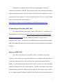
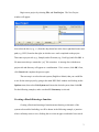
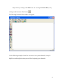
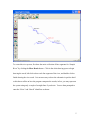
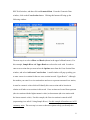
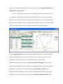
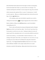
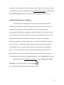
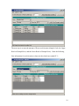
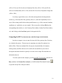
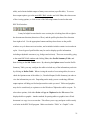
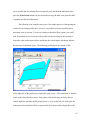
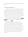
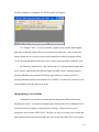
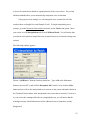
Some Basics of
HEC-RAS
River Analysis System
August 2006
Table of Contents
Downloading and Installing HEC-RAS .........................................................1
Purpose of HEC-RAS ......................................................................................1
Beginning a New Project .................................................................................2
Creating a Reach/Entering a Junction ................................................3
Adding Cross Section/Junction Data...................................................7
Adding Flow/Boundary Conditions .....................................................15
Saving the Data ......................................................................................18
Computing the RUN (steady/unsteady, subcritical/supercrictical/mixed) ...19
Viewing the Results ...............................................................................20
Error Messages, Warnings, and Notes ..........................................................23
Interpolating Cross Sections ...........................................................................24
ii
This manual is intended to aid the reader in performing many of the most
commonly used features of the HEC-RAS program quickly and with no prior knowledge
of how the program operates. All of the features of the HEC-RAS program are covered
in more detail in the program User’s Manual and the Hydraulic Reference Manual which
may be downloaded from the following site:
http://www.hec.usace.army.mil/software/hec-ras/hecras-document.html
Downloading and Installing HEC-RAS
As of August 2006 the most current version of HEC-RAS is 3.1.3, which may be
downloaded from the following site: http://www.hec.usace.army.mil/software/hecras/hecras-download.html (you may find this site quickly by typing “hec-ras
download” into Google.) The file size is 39.4MB and may be downloaded using either
high or low bandwidth; follow the directions at this site for downloading and running the
program.
Purpose of HEC-RAS
One of the major purposes for using HEC-RAS is to compute water surface
elevations. This is where Hydrology and Hydraulics come together; hydrology allows us
to calculate information such as 100-year flood flow, probable maximum flood flow
(PMF), etc., then using this information in HEC-RAS we can figure out what the possible
hydraulic conditions will be for a given study area. Therefore, knowing the water surface
elevation under various flow conditions can be helpful for many reasons, some of which
are: to evaluate possible flooding; for bridge/culvert design work; for riprap placement; to
1
determine construction risk; for obtaining permits from natural resource agencies; when
building structures such as bridges, culverts, homes, erosion control measures, etc., to
evaluate the differences in water surface elevation before and after construction in order
to comply with local, county, and FEMA regulations. HEC-RAS may also be used to
generate flow velocities for use in studying erosion and scour or for obtaining permits.
It is good to keep in mind that although a model will never be 100% correct, it
may still be useful. Greater confidence in a model may be gained through calibration,
comparing information collected on a particular project with corresponding data
computed by the model.
Beginning a New Project
To start the HEC-RAS program, double-click on the HEC-RAS 3.1.3 icon
located on your desktop, or go to the Start menu and click on all programs, HEC,
HEC-RAS, HEC-RAS 3.1.3. When the program opens, the main HEC-RAS window
will pop up on your desktop:
Many of the program features may be selected using the File, Edit, Run, or View menus,
or by using the list of buttons underneath these menus.
2
Begin a new project by selecting File, and New Project. The New Project
window will appear:
Next select the drive (e.g., c:\) from the drop down box in the lower right hand corner and
path (e.g., HEC) found on the right, in which to save work completed on the project.
Then enter a project title (e.g., Sample) and a file name (e.g., Prob1.prj) and click OK. A
file name must always contain the “.prj” file extension. A message box with the new
project title and directory will appear as a confirmation. If it is correct, click OK, if not,
click Cancel and complete the process again.
The next step is to select the unit system (English or Metric) that you would like
to use for the entire project by going to the main HEC-RAS window and clicking on the
Options menu, then select Unit System and choose the desired system, then click OK.
For the following examples, make sure that US Customary is selected.
Creating a Reach/Entering a Junction
Creating a Reach and entering a Junction means drawing a schematic of the
system to be modeled including, as will be shown in the following example, a junction
where a tributary meets a river, dividing the river into an upper reach and a lower reach.
3
Begin either by clicking on the Edit menu and selecting Geometric Data, or by
clicking on the Geometric Data button:
The following Geometric Data window will appear:
Use the following example to learn how to create a river system schematic; it may be
helpful to read through the entire process before beginning your schematic:
4
To create this river system, first draw the entire collection of line segments for “Sample
River” by clicking the River Reach button. Click in the white drawing space to begin
drawing the reach, left-click to draw each line segment of the river, and double-click to
finish drawing the river reach. It is not necessary to draw the schematic in perfect detail
as this has no affect on how the program computes the results, in fact, you may represent
the system using only a couple of straight lines if you desire. You are then prompted to
enter the “River” and “Reach” identifiers as shown:
5
In this case “Sample River” and “Upper Reach” are entered knowing that you will
include a tributary and a junction later.
The next step is to draw the tributary by using the same method for drawing the first river
reach; end the tributary by double-clicking where it connects with “Sample River.” The
following box will appear:
For the river name enter “Sample Creek,” and for the reach name enter “Tributary,”
then click OK.
Another message appears that asks if you want to split “Sample River” river on reach
“Upper Reach.” Click Yes and a new box appears to prompt you to enter a new reach
name below the split in the river as shown:
6
Enter “Lower Reach” and click OK. You are then prompted to enter a name for the
junction where the two reaches meet. Enter “Sample Junct” and click OK.
You may continue adding reaches (tributaries) and junctions using the process
above. You may also modify the existing river system by selecting from a list of choices
under the Edit menu of the Geometric Data window. If you make a mistake, you may
choose the Edit menu and select the option that allows you to delete a reach; then delete
any or all of the reaches that you may need to. It is a very good idea to continually save
your data. To save the geometric data, click the File menu on the Geometric Data
window, then click Save Geometry Data and enter a geometry data title such as “Base
Geometry Data.”
Adding Cross Section/Junction Data
After drawing the schematic of the system, you must enter the geometric data
(i.e., cross section and junction data) which the program will use to complete the
computations for water surface elevations, etc.
To enter the cross section data, go to the Geometric Data window as was done to
complete the river schematic. You do this by clicking on the Edit menu from the main
7
HEC-RAS window, and then click on Geometric Data. From the Geometric Data
window, click on the Cross Section button. Clicking this button will bring up the
following window:
The next step is to select a River and Reach (shown in the upper left hand corner). For
this example, Sample River and Upper Reach are selected to work with. In order to
enter cross section data you must select the Options menu from the Cross Section Data
window, and select Add a new Cross Section. A small window will pop up asking you
to enter a new river station for the new cross section in reach “Upper Reach.” Although
the number you enter for a river station does not have to represent an actual river station,
it must be a numeric value which will identify this cross section and its location in
relation to all other cross sections in this reach. Cross sections are located from upstream
(the river station with the highest numeric value) to downstream (the river station with
the lowest numeric value). For this example, the first river station is entered as 8.5
(representing river mile 8.5 along Sample River). For this example all numbers are in US
customary units. The next step is to enter a short description to help you identify this
8
cross section from among the other cross sections later. Type in upstream boundary of
Sample River, Upper Reach.
Now we can begin to enter the cross section data (station and elevation data, or XY coordinates). This data is entered from the left bank of the cross section to the right
bank of the cross section (the left side of the cross section will have lower numbers than
the right side) as though you were looking in the downstream direction, or in the direction
of flow. For this example, enter the numbers as shown in the following figure:
Click the Apply Data button (top center) when finished to generate a cross section plot.
If this plot matches your cross section data, then you are ready to enter the rest of the
information in the boxes shown just to the right of where you entered the
Station/Elevation data. Next, enter the Downstream Reach Lengths (left over bank,
main channel, and right over bank), which is the length from this cross section to the next
downstream cross section. Enter the corresponding Mannings’s n Values (for a
description of these roughness values, click the small question mark to the right of the
Manning’s n Values title block). Next, enter the Main Channel Bank Stations. The
9
Main Channel Bank Stations delineate the left and right over bank areas (flood plains)
from the main channel and will show up as red dots on the cross section plot. The
Contraction and Expansion coefficients are used to compute the energy losses associated
with the contraction and expansion of flow in a system. For most projects, 0.1 and 0.3
are used, respectively. When you are finished entering the data as shown in the previous
figure, click the Apply Data button.
A file containing a picture may also be linked to a particular cross section by
clicking on the camera button:
choosing the appropriate River, Reach, and River
Station, and then by clicking on the Add Picture button to search for and add the
corresponding picture file.
There are other useful options for entering and editing data found by clicking the
Options menu of the Cross Section Data window. We will use the Copy Current Cross
Section option to create the next cross section. Copying an existing cross section will
simply copy all of the existing data exactly as it is, you must then modify the copied cross
section data as needed (e.g., river station number, station/elevation data, etc.). The
advantage of this option is that it allows you to interpolate a new cross section, or to copy
an existing cross section which can be modified quickly using choices listed in the
Options menu. Select Copy Current Cross Section and enter the next river station
which is 8.25, then click OK. For this example, modify all of the cross section
information to match the following figure, adding station/elevation data as necessary:
10
The Downstream Reach Lengths are left blank in this case because the length between
the upstream and downstream reach includes the junction where the tributary (Sample
Creek) flows into “Sample River,” and this length will be entered later as Junction Data.
Click the Apply Data button when finished to generate the cross section plot.
We must now enter upstream and downstream boundary cross section information
for the “Lower Reach” of Sample River and for “Sample Creek.” First, select Sample
River from the River drop down box (upper left hand corner) on the Cross Section Data
window and Lower Reach from the Reach drop down box. Next click on the Options
menu and choose the Add a new Cross Section option. For this example, enter 7.5 as
the new river station and click OK. Type in upstream boundary of Sample River,
Lower Reach as the description. Next, enter the following cross section information as
shown:
11
Click the Apply Data button when finished.
Repeat the previous procedure to add a cross section (you may use the Copy
Current Cross Section option) at the end of the Lower Reach of Sample River and use
the following river station, description, and cross section information as shown:
12
Since this is the downstream boundary of Sample River, the Downstream Reach Lengths
are entered as zero or they may be left blank. If you choose the Copy Current Cross
Section option, you may more easily duplicate the next cross section for this example by
modifying the existing elevations. This is done by clicking Options, Adjust Elevations,
type -0.2, and click OK.
Next, enter the following information for the upstream cross section of the
“Tributary” of “Sample Creek”:
Click the Apply Data button when finished, and then enter the following information for
the downstream cross section of “Sample Creek”:
13
Click the Apply Data button when finished.
The final step in this example is to enter the junction data. This is done by first
going to the Geometric Data window and clicking on the Junction button:
The Junction Data window will appear; enter the following information to indicate the
lengths across each section of the junction:
The Energy computation mode is already selected which means that the energy equation
will be used to model the junction. If the Momentum computation mode (momentum
14
equation) is used, the angle at which the tributary enters will have to be entered. Finally,
save the geometric data by clicking File on the Geometric Data window, and then choose
Save Geometry Data to update the geometric data saved previously (see page 7).
Adding Flow/Boundary Conditions
The amount of flow through the system must be entered along with certain
boundary conditions before running the program to compute the desired results. The
amount of flow through a system will depend on the type of study conducted.
Determining which boundary conditions are required depends on the conditions of the
system and the type of model being run. The options for running the model are steady
and unsteady flow analysis, and within each of these are options for modeling a
subcritical, supercritical, or mixed flow regime. As stated in the HEC-RAS Hydraulic
Reference Manual, “subcritical profiles computed by the program are constrained to
critical depth or above, and supercritical profiles are constrained to critical depth or
below. In cases where the flow regime will pass from subcritical to supercritical, or
supercritical to subcritical, the program should be run in a mixed flow regime mode.”
For this example we will perform a steady flow analysis using a subcritical flow regime.
Begin by going to the main HEC-RAS window, click on Edit and then Steady
Flow Data, or click on the steady flow data button:
This will bring up the following steady flow data window:
15
The next step is to enter the amount of flow at each location (Sample Creek, the Upper
Reach of Sample River, and the Lower Reach of Sample River). Enter the following
flow information for each location as shown in the white boxes under PF 1:
16
Click the Apply Data button (upper right hand corner) when finished. The heading PF 1
may be changed to represent the event that this amount of flow represents (e.g., 100yr, or
PMF, etc.). Also, more flow profiles may be added by increasing the number of profiles
to allow you to model more than one event at a time.
Next, we need to enter the necessary reach boundary conditions in order to
establish the starting water surface at the upstream and downstream ends of the system
and enable the program to begin calculations. For a subcritical flow regime, boundary
conditions are only necessary at the downstream end; for a supercritical flow regime,
boundary conditions are only necessary at the upstream end; and for the mixed flow
regime, boundary conditions are necessary for both the upstream and downstream ends of
the system. Boundary conditions at junctions are considered internal and will already be
listed in the steady flow boundary conditions table. Click on the Reach Boundary
Conditions button on the steady flow data window to view the Steady Flow Boundary
Conditions table:
17
The five options for entering boundary conditions are: know water surface elevations;
critical depth (when selected, the program will calculate critical depth for each of the
profiles and use that as the boundary condition); normal depth (an energy slope must be
entered which is used to calculate the normal depth at that location using Manning’s
equation); rating curve (an “elevation versus flow” rating curve must be entered from
which the program interpolates the water surface elevation for each profile given the
flow).
For this example, click on the Downstream box for the “Lower Reach” of
“Sample River,” shown highlighted in the previous figure. Click the Normal Depth
button (top center) and enter 0.02 as the energy slope, then click OK. Click the OK
button of the Steady Flow Boundary Conditions window, and you will be brought back to
the Steady Flow Data window. Click the Apply Data button (top right hand corner) to
allow the program to accept all the input data. The final step is to save the flow/boundary
conditions data. From the Steady Flow Data window, click File, then click Save Flow
Data and enter a title such as “Base Flow Data,” and click OK. This completes the
process for entering the flow/boundary conditions data.
Saving the Data
At this point, we have indicated how to save the different files of a HEC-RAS
project as we have covered each section. The complete list of files that can make up a
HEC-RAS project are: one project file (.prj); one file for each plan (.P01 to .P99); one
run file for each plan (.R01 to .R99); one output file for each plan (.O01 to .O99); one file
for each set of geometry data (.G01 to .G99); one file for each set of steady flow data
18
(.F01 to .F99); one file for each set of unsteady flow data (.U01 to .U99); one file for
each set of sediment data (.S01 to .S99); and one file for each set of hydraulic design data
(.H01 to .H99).
It is always a good idea to save a file after entering the data for that particular
section (e.g., the steady flow data, geometry data, etc.), and more importantly to save a
copy of the existing model before making modifications (e.g., to flow amounts, boundary
conditions, etc.) and before you run a model. Files are saved by clicking File from the
corresponding data window (i.e., the Geometry Data window, Steady Flow Data window,
etc.) and clicking on the Save Data option for that particular file.
Computing the RUN (steady/unsteady, subcritical/supercrictical/mixed)
In order to compute a run you must first enter all of the geometry data, flow data,
etc. related to the project. The next step in computing our steady flow analysis is to
define a Plan. If there are multiple files for a project, the plan defines, for instance,
which geometry and flow data are to be used for the run and allows you to enter a
description and short identifier to quickly access the correct output files and other run
information later on.
To create a plan for this example, go to the main HEC-RAS window and click on
Run, and then click Steady Flow Analysis, or click the steady flow analysis button:
to open the Steady Flow Analysis window:
19
Since we only have one geometry and steady flow file, we may leave these files as they
appear in the Steady Flow Analysis window. To create a new plan, click File, and then
click New Plan, and enter a name for the plan such as “Sample Plan,” and click OK.
You are then asked to enter a short identifier for this particular run, enter “Sample Run,”
and click OK. When you are conducting multiple runs, it is important to enter a short
identifier that will help you to quickly locate a particular plan when viewing multiple
plan output from the graphics and tables. You may also type in a description of the plan
in the space provided. Since the Subcritical Flow Regime is already selected, click File
and then Save Plan. Finally, to perform the steady flow calculations, click the
COMPUTE button and allow the program to compute the results of the run, and then
click the Close button on the pop-up window.
Viewing the Results
After computations have finished successfully, you have several options for
viewing output, they are: cross section plot; profile plot; general profile plot; rating curve;
X-Y-Z perspective plot; detailed tabular output at a specific cross section (a cross section
20
table); and a limited tabular output of many cross sections (a profile table). To access
these output options, go to the main HEC-RAS window and click View, then choose one
of the viewing options, or click on one of the following buttons located on the main
HEC-RAS window:
It may be helpful to note that the cross section plot is looking from left to right in
the downstream direction (direction of flow), and the profile plot shows flow direction
from right to left. Use the appropriate buttons and drop down boxes on the profile
windows to cycle between rivers/reaches, and to include/exclude certain rivers/reaches in
a plot. Several types of profile tables may be used to display specific information,
including at hydraulic structures (e.g., bridges and culverts). These are accessed by going
to the main HEC-RAS window and clicking View, then Profile Summary Table, and
then clicking on the Std. Tables menu. By choosing the Options menu from the Profile
Summary Table, you may configure the table to include any of the information you desire
by clicking on Define Table. When viewing the results of a run using tables, be sure to
check the Options menu of the tables (i.e., Detailed Output, Profile Summary) in order to
view the information you seek. Depending on the study you are conducting, different
output options will help you find and present the results you need. Tables and graphics
may also be sent directly to a printer or to the Windows Clipboard to add in a report. To
select these options, click either Print or Copy to Clipboard on the File menu of the
displayed table or graphic. Another method for pasting tables or graphics into a Word
document is to copy it as a screen shot. This allows you to copy and paste a table exactly
as it looks in the HEC-RAS program. Make sure that the “Table” or “Graphic” is the
21
active window (the last window that you opened), press and hold the Alt button, then
press the Print Screen button (on your keyboard) to copy the table, next paste the table
or graphic into the Word document.
The following is an example (not a part of our sample project) of interpreting the
results of a run using a profile plot. It may be very helpful to look at a profile plot to
determine areas of concern. If you were running a subcritical flow regime, you could
look for potential areas of concern on the profile plot by searching for the location(s)
where the water surface passes above and below the critical depth, which may indicate
the location of a hydraulic jump. The following profile plot is an example of this:
At the right side of the profile plot, a hydraulic jump occurs. This is indicated by the blue
water surface line (flow direction is from right to left) which starts out below the red
critical depth line and then quickly jumps above it. Over on the left side of the plot, the
water passes from subcritical flow to supercritical flow (water surface begins above the
22
red critical depth line and then passes underneath it). The green line indicates the energy
grade line.
Error Messages, Warnings, and Notes
After computing a run, you should always check if the program has generated any
error messages or warnings. These messages may help you to figure out how to get the
program to complete a run or suggest ways by which you can help the program to
generate more accurate results. Whenever a warning message is generated, you should
review the hydraulic results at that location to make sure they are reasonable, and if they
are then the message may be ignored. If the results are not reasonable, you will probably
need to take action to make the warning message disappear from future runs.
To view the complete table of error messages and warnings, go to the main HECRAS window and click the View menu, and then click on Summary Err, Warn, Notes,
or click on the appropriate button:
Many warning messages are caused by bad or inadequate data. Common
problems that cause warning messages to occur are: cross sections are spaced too far
apart; the starting and ending stations of cross sections are not high enough (the
computed water surface is higher than either end point of a cross section); a bad starting
water surface elevation (a boundary condition is specified that is not possible for the
specified flow regime); bad cross section data can cause many problems (most often the
program cannot balance the energy equation and will default to critical depth); notes
(these messages provide information about how the program is performing the
computations).
23
From the example we completed, the following table will appear:
For “Sample Creek,” we can see that the computed water surface started higher
than either of the end points of the cross section at river station 8.0. Also, because the
energy change due to velocity (velocity head) changed more than the program default
(0.5ft), the program indicates that more cross sections may be needed for Sample Creek.
By choosing “Sample River” and “(All Reaches),” to include both the upper and
lower reaches, from the drop down boxes (upper left hand corner), warnings indicate a
need for additional cross sections for both the upper and lower reaches as well as a
message indicating that the normal depth at river station 7.0 on the lower reach was set to
critical depth because the slope is too steep.
Interpolating Cross Sections
Additional cross sections are often needed to adequately model friction losses
throughout a system. A common warning message indicates the need of additional cross
sections because the change in velocity head is too large. There are three ways to
interpolate cross sections in HEC-RAS. The first is to copy an existing cross section and
then adjust the station and elevation data, the cross section data editor allows you to raise
24
or lower elevations and to shrink or expand portions of any cross section. The second
and third methods allow you to automatically interpolate cross section data.
Using our previous example, we will interpolate cross sections for all of the
reaches (those on Sample River and Sample Creek). To begin interpolating cross
sections, go to the Geometric Data window and click on the Tools menu option. Move
your cursor over XS Interpolation and click on Within a Reach. You will notice that
you also have the option to interpolate cross sections between two selected existing cross
sections.
The following window appears:
Choose “(All Rivers)” from the first drop down box. Type in 20 as the Maximum
Distance between XS’s, and click the Interpolate XS’s button. Next click the Close
button and you will see the interpolated cross sections on the system schematic shown on
the Geometric Data window; each interpolated cross section has an asterisk (*) next to it.
As you review the warnings table after re-computing the run, you will notice that the
warning messages which indicated a need for additional cross sections have mostly
disappeared.
25