1
Page 1
Users Guide for the Meshparts
Software
1 System Requirements
The MESHPARTS Software in the current version runs only on Windows operating systems.
The software was tested on Windows XP and Windows 7 (64 Bit and 32 Bit). There is no
special requirement regarding the memory amount and processor speed but with bigger
finite element models more memory will be needed.
2 Download
The software can be downloaded from www.meshparts.de/software
3 Quick start guide
1. Go to www.meshparts.de/software and download the latest release of the MESHPARTS
Software.
2. Save the executable on your hard drive (preferable on C:\, D:\ or other short paths) and run
it as an administrator (Windows context menu for executable files). On a Windows 7
operating system the graphical user interface (GUI) looks like this:
Page 1
Page 2
3. Click on “Register as a new user” and create a new account by registering with your e-mail
address and a password (additional information required). After submitting your data, you
will receive a confirmation e-mail. Click on the link in the e-mail.
4. Login with your e-mail address and password (same as used for registering on step 3):
5. Check the server response in the message window. You should see a similar message and a
question to setup the offline library:
6. If you log in for the first time and the offline library is not set yet, you should click on “Yes”
in order to set the offline path for www.meshpart.de, as this step is very important for the
proper functioning of the software.
4 Your first Finite Element Assembly
The MESHPARTS Online Library of parametrical finite element models is directly accessible
from the MESHPARTS Software. This allows users to create directly finite element assemblies
without having a local geometry meshing software installed.
1. In the explorer tree right click on a folder of your choice and choose from the context
menu New assembly. The new assembly opens automatically.
If you already set up the path to the offline library as described in Chapter 3, you can skip the
steps 2 and 3.
2. Select from the explorer tree the path https://www.meshparts.de
Page 2
Page 3
3. In the Offline Library frame, set the path to your offline library (browse to the path and
click on "OK"). All models downloaded from the online library will be mirrored to this path.
4. Browse in the explorer tree to
https://www.meshparts.de/StandardComponents/FreeExamples/BallScrewSpindle/BallScrewS
pindle_3D_500_30_50_50_50_50_20_20_15_15_40_40_1.0.cdb (you can also copy and paste the
path into the path field above the explorer tree)
5. Right click the model and select "Download"
Page 3
Page 4
6. Drag and drop the downloaded model to the model tree of the new assembly.
Drag & Drop
7. Repeat steps 4, 5 and 6 for the model
https://www.meshparts.de/StandardComponents/FreeExamples/Bearing/Bearing_SS_20_50_1
5_0_200_300_0_0_0_0_1.0.cdb.
Your new assembly looks like this:
Page 4
Page 5
8. Scroll to the right in the model tree and change the number of part instances of the
bearing from 1 to 2 by choosing "Rename" from the context menu.
9. From the model tree select the nodal sets BALLSCREWSPINDLE_BEARINGSEATL_1,
BALLSCREWSPINDLE_BEARINGSEATR_1 and BEARING_INNERRING_1. Alternatively, you can
also select surfaces directly on the 3D model but selecting nodal sets is more robust with
respect to model changes. Hold down the control key in order to make a multiple selection.
Page 5
Page 6
10. With one click on the second button in the "Define new relation" frame, define a new
contact relation between the selected nodal sets.
11. From the model tree select the nodal sets BALLSCREWSPINDLE_BEARINGSEATL_0,
BALLSCREWSPINDLE_BEARINGSEATR_0 and click on the right arrow in the "1st multiple
selection" box:
12. From the model tree select the nodal set BEARING_ORIG and click on the right arrow in
the "2nd multiple selection" box:
Page 6
Page 7
13. With one click on the first button in the "Define new relation" frame, define a new
positioning relation between the selected nodal sets.
Your assembly is now fully defined and looks like this:
Page 7
Page 8
5 Exporting Finite Element Assemblies
MESHPARTS finite element assemblies are exported (converted) into a file format that can be
read by third-party finite element software. Currently the Ansys® specific CDB file format is
supported. Ansys® CDB models can also be imported into Abaqus®.
In most cases, you will want to open the MESHPARTS assemblies with a third-party finite
element software in order to post-process the finite element results. The pre-processing and
the solution setup you can perform directly in the MESHPARTS software.
1. In order to export MESHPARTS assemblies to Ansys® CDB format select an assembly item
in a model tree and click on the button
:
The new exported model will appear as a child item of the assembly file in the explorer tree
(click on the plus sign if necessary).
2. Right click on the exported model and choose "Open with native FE program". The model
opens in Ansys® Workbench or Mechanical APDL (depending on the program settings).
Page 8
Page 9
6 Meaning of icons
In order to work with the MESHPARTS Software it important to know the meaning of the
icons used.
This is an operating system folder on your local or network drive.
This is a folder from the online library.
This is a macro file (e.g. Ansys® APDL macro library with MESHPARTS specific
structure). From macro files, model files are generated and grouped as child items under the
macro item.
An orphan model file (part); the origin of the model file is unknown.
A model file generated from a MESHPARTS macro file.
A model file generated from a MESHPARTS assembly file.
A MESHPARTS assembly file. An assembly file contains definitions of assemblies that
can consist of model files or other assembly files.
Page 9
Page 10
A macro generated model file that you should re-generate or download, because it is
older than the macro file or online version respectively.
An assembly generated model file that you should re-generate or download, because
it is older than the assembly file or online version respectively.
An assembly file that you should re-download, because it is older than the online
version.
An orphan model file from the online library that is also available in your offline library.
A macro generated model file from the online library that is also available in your
offline library.
An assembly generated model file from the online library that is also available in your
offline library.
An assembly file from the online library that is also available in your offline library.
A macro generated model file whose macro file is not available anymore.
This is an assembly generated model file whose assembly file is not available anymore.
An orphan model file that is not available anymore.
A macro generated model file that is not available anymore.
An assembly generated model file that is not available anymore.
Page 10
Page 11
7 Changing the viewing angle, zooming, and panning
In order to change the viewing angle, zooming, and panning of your models you will need a
mouse with three buttons (left, right and middle button) and a scroll wheel. For panning the
model view, you will need a keyboard.
Change the viewing angle of your model: Hold down the middle button on your
mouse while moving the mouse horizontally and vertically.
Zoom in and out: Turn the mouse wheel up and down.
Pan your model horizontally and vertically: Hold down the control key on your
keyboard and the middle button on your mouse while moving the mouse horizontally
and vertically.
The actions described above base on the current mouse position relative to the model. Also,
consider following two point, when rotating the model:
If the drag operation begins with the mouse positioned over the model, the rotation
point is the intersection point of the viewing direction with the model.
If the drag operation begins with the mouse positioned beside the model, the
rotation point is the center of the model.
7.1 Predefined views
On the upper-right corner of the model viewing area, you can find eight buttons for setting
predefined viewing directions and zooming.
From the left to the right following predefined settings are available:
1. Isometric view
2. Front view (negative x axis direction)
3. Back view (negative x axis direction)
4. Right view (negative y axis direction)
5. Left view (negative y axis direction)
6. Top view (negative z axis direction)
7. Bottom view (negative z axis direction)
8. Fit model into the viewing area
9. Restore last exploded view
7.2 Exploded views
When different models in an assembly overlap or share common surfaces, it is more difficult
to make selections. A recommended way to overcome this difficulty is to create an exploded
view of your assembly.
Page 11
Page 12
You can create exploded views very fast by simply dragging away different models or
assemblies with the left mouse button (hold down the left mouse button and move the
mouse).
Additionally, single parts or assemblies can be rotated by dragging the mouse while holding
the right mouse button pressed. Per default, the rotation takes place around the origin of the
part or assembly. If you hold down the CTRL key while dragging the mouse, rotation will take
place around the selected point on the model.
If you hold down the shift key while dragging the mouse (either left or right button), then the
part deepest available in the assembly hierarchy will be translated or rotated. Of you do not
use the shift key, then the part or assembly, which is a direct child of the main assembly, will
be translated or rotated.
7.3 Wireframe, smooth and section views
Directly over the 3D viewing area, you can find four further buttons that will change the way
your model or assembly looks like:
Wireframe: Only curves and other selected geometry elements are visible.
Smooth surface: The mesh edges are invisible.
Translucent surface: The mesh faces are 25% opaque.
Transparent surface: The mesh faces are 0% opaque.
Section view: The model or assembly is cut with the selected geometry element of
type “PLANE”.
Section view reversed: Same as above, but the planes normal direction is reversed.
8 Selection of geometric entities
There are five types of geometric entities available for selection:
1. Models (e.g. Ansys CDB models)
2. References (model origin, Cartesian axes, Cartesian planes)
3. Nodal Sets (groups of finite element nodes)
4. Surfaces (planes, cylinders, spheres)
5. Curves (lines, circles)
6. Points
The model origin, Cartesian axes and planes are threated a points, lines and planes
respectively.
Page 12
Page 13
You can select geometric entities by one single left mouse click. Holding down the control
key on your keyboard enables you to select multiple geometric entities at the same time.
Selected entities change their color to green.
There are two possibilities for selecting geometric entities:
1. Selection from the model tree
2. Direct selection on the model
The selection from the model tree is a very convenient way to select entities if you know their
names (e.g. nodal sets).
The direct selection on the model is the best way to select geometric entities if you do not
know their names.
In some cases, when the bounding boxes of two or more geometry entities overlap, more
than one entity is found by a select operation. In those cases, there are three possibilities in
order to choose the right entity:
1. Repeated clicks on the same position will cycle through all selectable entities
2. Right click on the model and choosing a geometric entity from the context menu.
3. Drag with the left mouse button some models away from their original position in
order to get better access to the geometry entities you want to select.
8.1 Selection filter
On the upper-left corner of the model viewing area, you can find six buttons for filtering the
selection of specific geometric entities.
From the left to the right following filters are available:
1. Model filter (select only models)
2. References filter (select only references)
3. Nodal set filter (select only nodal sets)
4. Surface filter (select only surfaces)
5. Curve filter (select only curves)
6. Point filter (select only points)
The behavior of the selection filter in the toolbar is additive. This means, that you have to
explicitly activate and deactivate each filter option manually.
Another way of changing the selection filter is to show a context menu by a right click on the
3D area. The context menu also shows the corresponding key shortcuts.
Page 13
Page 14
The behavior of the selection filter in the context menu is exclusive. This means, that
activating a filter option, will automatically deactivate all other filter options. Nevertheless, if
you hold down the CTRL key while choosing a filter option, the filter will behave additive.
8.2 The find function
In some cases, you want to select some geometry items that have a specific name. Instead of
selecting the items one by one, you can use the Find function from the context menu or by
pressing CTRL+F in the model tree:
In the example above, we have the FE assembly of a ball screw drive and we want to select
the nodal sets beginning with KGM_KUGEL and ending with _1. We can input the search
criteria KGM_KUGEL*_1 (the asterisk is a placeholder for any characters) into the search field
that opens when you activate the Find function:
The search starts by pressing Return or by clicking in the "Find" button. The found items are
then automatically selected in the model tree.
Page 14
Page 15
You can also use the Find function in order to find files or folders in the explorer tree. In that
case, make sure that the explorer tree is the active tree by clicking inside it and selecting the
folder where you want to start searching.
The Find function always refers to the selected folder. If nothing is selected the search is
performed over all available folders. Searching over a computer volume or even all available
volumes can require up to several minutes of time.
If you press the CTRL key while the Find function is started, the found items are added to the
previous selection.
9 Measuring distances and angles
It a common task to measure the distance or angle between two surfaces or other geometric
entities.
In the MESHPARTS software you can select two geometry entities from the model tree or
directly on the 3D viewing area in order to measure (if applicable) the distance and angle
between them.
Page 15
Page 16
Distances are valid for following combinations:
Point-Point
Point-Line
Point-Plane
Point-Sphere (center)
Point-Cylinder (middle axis)
Point-Circle (normal axis through the center)
Line-Line
Line-Sphere (center)
Line-Cylinder (middle axis)
Line-Circle (normal axis through the center)
Plane-Plane (if parallel)
Angles valid for following combinations:
Line-Line
Line-Cylinder (middle axis)
Line-Circle (normal axis through the center)
Plane-Plane
10 Defining relations between models
A relation between two models can be of two types:
1. Positioning
2. Connection
Page 16
Page 17
In order to define a positioning and/or a constraint you must select at least two geometry
entities and then click on one of the three buttons in the “Define new relation” frame:
You can also define multiple relations at the same time. For that select multiple geometry
items and place the selection into the multiple selection fields.
Choose how to create relations pairs using the two multiple selections:
The "Combine pairs" option combines the first item in the first multiple selection with
the first item in the second multiple selection. The same will apply to the second items
and so on. If one multiple selection contains less items than the other one, the
creation of pairs stops the last possible pair.
The "Combine all" option generates all possible combinations of two geometry items.
Use this option with caution as it can create a huge amount of new relations.
10.1 Positioning constraints
Positioning constraints are geometric constraints between pairs of models in order to define
their relative position. You can select any combination of
Lines
Circles
Planes
Cylinders
Spheres
in order to define a positioning constraint.
A positioning constraint can be of three types:
Distance (in model length units)
Angle (in degrees)
Tangent
A distance constraint implies that the angle between the direction vectors of the geometric
entities is zero.
Page 17
Page 18
The type of a positioning constraint can be set up in the “Positioning properties” frame by
selecting one of the positioning items in the model tree:
In addition to the type of a constraint, the direction of a constraint can be reverted with the
help of the "Reverse" option.
The "System" option is only valid for positioning constraints between two points. This will
also constrain the coordinate systems of each point to have the same orientation of their
axes.
10.2 Connections
Connections define a physical interaction between two geometry entities (e.g. contact). You
can define one of the following connection types:
surface-surface
curve-surface
point-surface
curve-curve
point-curve
point-point
Most of the connections are modeled per default by bounded penalty contact (similar to
gluing). Point-point and point-curve connections modeled per default by constraint
equations. Other contact options are available when you select a specific connection item in
the model tree:
Page 18
Page 19
You can read more about each contact option in the Ansys® User’s Manual under // Contact
Technology Guide // 3. Surface-to-Surface Contact // 3.9. Set the Real Constants and Element
KEYOPTS.
10.3 Changing the geometry items in a relation
If you want to change one or both geometry items in a relation (positioning or connection),
select the corresponding relation item in the model tree and click on “Choose other
geometry” in the relation properties frame on the right side of the window.
11 Applying loads and boundary conditions
You can apply loads and boundary conditions (LBCs) to all type of geometry items available
with the exception of reference planes (XY, YZ and ZX items) and reference axes (X, Y, Z
items).
On surfaces or equivalent nodal sets, LBCs are applied through external points (pilot nodes)
that connect to the surfaces through Multi Point Constraints (MPC).
Page 19
Page 20
On curves and points or equivalent nodal sets, LBCs act on every single node of the mesh
associated with the geometry. Please take into account, that nodal loads and nodal BCs are
defined in the node coordinate system. In MESHPARTS if a model is rotated then also the
node coordinate system are rotated and so the LBCs.
On Origin items you can apply loads of following types in the global coordinate system:
Linear acceleration
Rotational acceleration
Linear velocity (as initial condition)
Rotational velocity
If you are applying a linear velocity to an Origin item, the velocity is considered as an initial
condition, meaning it should only be applied in the first load step.
You can apply an acceleration or velocity to subparts of an assembly by selecting the related
Origin items. If you select the origin item of the main assembly, then accelerations and
velocities are acting on all subparts of the assembly.
In order to apply LBCs, select the geometry first and then click on one of the buttons “New
load” or “New BC”:
In the “Loads and Boundary Conditions properties” frame you can then specify the amount
of load or displacement for each individual degree of freedom. These values have only
effect in the first time step of a simulation.
Page 20
Page 21
When applying only loads to a surface, the surface behavior can be flexible or rigid. You can
change this behavior from the “Loads and Boundary Conditions properties” frame:
For surface loads and boundary conditions, a pilot node is automatically created at the center
of the surface bounding box. For more control over the location of the pilot node, you can
input your own coordinates relative to the global coordinate system:
Page 21
Page 22
In some cases (harmonic analysis), you need to define a phase angle for a LBC. In
MESHPARTS you simply input both amplitude and phase (in degrees) as numbers separated
by one white space into the fields of each degree of freedom:
You can specify LBCs for more than one time step and the number of sub-steps for each
time step using the “Load step editor” and “Time stepping” frames:
Page 22
Page 23
In the “Load step editor” frame, you can select a load or boundary condition curve and add a
new point by double-clicking on a straight segment of the curve. You can delete a point by
a right click on that point.
Furthermore, you can shape the curves by dragging points or straight segments horizontally
or vertically. By holding down the shift key when dragging, the drag resolution increases. You
can double-click in the top-left corner of the editor and enter the exact x/y coordinates of
the point.
You can change the limits of the axes (time/frequency/amplitude) by a double click on
them. By changing the upper time or frequency limit, all time points will scale accordingly so
that the LBC curves will fit the new time interval.
Lastly, you can import tabular data from an Excel-Table, text file or similar format. For
example, in Excel you select the table area of interest and press CTRL+C to copy it. Then
select one or more LBC items and click on the “Paste” button in the Load step editor frame.
Click on the “Save” button in the Load step editor frame. The pasted tabular data should have
one column for the time and six columns (in general six DOF) for each selected LBC item. So
for example if you have two LBC items you will need a table with 1+2x6=13 columns.
Page 23
Page 24
12 Adding discrete joints to an assembly
Typically, discrete joints are formed by two nodes that span a discrete stiffness and/or
damping element. Many model components from the Meshparts library already contain
discrete joints. These are needed to efficiently model the behavior of linear guides, bearings,
ball screw nuts etc.
You can also add discrete joints to FE assemblies rather than to model components. This
method is recommended for special FE assemblies that cannot be easily or do not need to be
standardized.
Discrete joints are available in the properties frame of defined connections or LBCs. For
connections, discrete joints can only be defined if the connection contains surfaces or points.
For LBCs, joints can be added to any type of geometry (surfaces, curves and points).
In the following example joint stiffness is added to the outer ring surface of a bearing by
selecting the corresponding LBC item in the model tree.
0.0 0.0 10e-6 100e6 20e-6
250e6
Joint stiffness and damping can be linear or nonlinear. You can define a joint with linear
stiffness or damping by a single value (the stiffness or damping coefficient). Nonlinear joint
behavior you can define by inputting displacement-force (stiffness) and velocity-force
(damping) pairs, as in the above example for the joint stiffness in the Y degree of freedom.
Make sure that the value pairs always contain the origin point (0 0).
In order to add a discrete joint to a LBC, Meshparts internally defines a second node on the
same location as the LBC node and attach the discrete stiffness, damping and mass elements.
The load or boundary condition is then actually applied to the second node, not to the LBC
node (as in the case without added discrete joint).
In the case of a LBC applied to a surface, the added discrete joint is inserted between the LBC
node and the pilot node of the contact surface:
Page 24
Page 25
Contact surface
Pilot node
LBC node
Discrete joint
In the case of a LBC applied to a curve, multiple discrete joints are inserted between each LBC
node and each curve node. The defined stiffness, damping, mass are equally distributed to
each joint:
Curve nodes
LBC nodes
Discrete joints
If you add a discrete joint through a connection item, you can not only define mass, stiffness
and damping, but also a transmission factor for up to six degrees of freedom combinations
(translations and rotations).
Pay attention to the fact, that the degrees of freedom of the joint are defined in the
coordinate system of the assembly that directly contains the joint. If the assembly containing
the joint is inserted in another assembly with different orientation, then the joint properties
will also adapt to the new orientation.
In the following example, a screw like behavior is defined between the surfaces of two parts
along with a linear discrete stiffness and mass equally distributed to the two surfaces:
Page 25
Page 26
The screw like behavior is defined in the first degrees of freedom pair as “RX to UX”, meaning
that the relative translation in X is related to the relative rotation about X by a factor that is
input as a parametric expression
ℎ
,
2𝜋
where ℎ is the thread slope of the screw.
For joints with added transmission, the order of the joint interfaces as it appears in the
relation name is very important: first interface, transmission, Spring/Damper, second interface
(see below an exploded view of an assembly with added joint).
Spring
Damper
Transmission
Point mass
First interface
Second interface
12.1 Nonlinear stiffness
If the nonlinear stiffness of a joint contains only the tensile curve (positive values), the
compressive curve (negative values) will be automatically computed by reflecting the tensile
curve.
Page 26
Page 27
If the nonlinear stiffness of a joint should offer no resistance to compressive loading, then the
compressive of the curve should be formed by just one displacement-force pair (typically -1.0
0.0). Thus, a nonlinear spring that offers no resistance to compressive loading could be input
in this way: -1.0 0.0 0.0 0.0 10e-6 100e6 20e-6 250e6 30e-6 400e6
13 Solving a FE assembly
After you define positioning and connection relations and apply loads and/or boundary
conditions to an FE assembly, you can obtain a solution of the current FE assembly by
selecting the assembly item in the model tree. Select a type of analysis (static, modal
harmonic or transient) and click on the solve button:
If you want to setup more options select one of the supported solvers (currently Ansys) from
the “Solution settings” in the main menu:
In the new window select the type of analysis you want to set-up (static, modal, harmonic or
transient) and adapt the available parameters:
A more advanced feature is the specification of (pre-/post-) solution macros. This way you
can perform special operations on your model using the integrated scripting language of the
Page 27
Page 28
third party solver (e.g. APDL – Ansys Parametric Design Language). You can setup four
different macro paths in the “Assembly macros” frame:
A macro that will be executed before the assembly is solved.
A macro that will be executed before each time step of the assembly solution.
A macro that will be executed after each time step of the assembly solution.
A macro that will be executed after the assembly is solved.
Important! For Ansys models (assembled cdb models), all assembly macros are executed
during the solution phase. If you are performing pre-processing operations in one of the
solution macros, you have to explicitly enter the pre-processor at the beginning of the macro
(/prep7 command) and explicitly enter the solution at the end of the macro (/solu command).
You can solve one or more assembled models also directly from the explorer tree. Select
one or more assembled model files and choose “Solve” from the context menu. This second
method of solving assembled models does not require the corresponding assembly to be
open. It also have the advantage over the first method that you can schedule multiple
simulations with just one click. The models will then be solved sequentially, one after one:
14 Post-processing the results
At the current software current release, MESHPARTS does not provide integrated postprocessing (evaluating displacements, stresses etc.) of the FE results. Instead, you can right
click an exported model file in the explorer tree and choose “Open with Ansys Workbench”,
“Open with Ansys MAPDL” or “Open with Abaqus CAE”. You can then perform the postprocessing using the native FE program.
Page 28
Page 29
15 Working with assembly equations
In many situations, there exists a relation between the parameters of different models or
distances of some positioning constraints. In such cases, you can simplify your workflow and
accelerate model changes by defining equations that describe the relations between different
model parameters of an assembly.
To do so, select an assembly item in the model tree and write new equations or edit available
ones in the “Assembly equations” frame:
2. Write, edit
equations
1. Select an
assembly in
the model tree
3. Save and
apply changes
The syntax of an equation is:
ParameterName = Expression
The parameter names are case sensitive. Do not use empty spaces or special characters in
parameter names.
The expression on the right side of the equal sign of an equation can describe:
a mathematical expression
a string
By clicking on the “Save and apply equations” button, the assembly equations are evaluated
and entities linked to these parameters are updated accordingly.
15.1 Using mathematical expressions
In mathematical expressions you can use:
Page 29
Page 30
numbers
other predefined parameters
operators (+, -, *, /, **, %)
parentheses
functions (abs, sin, cos, tan, asin, etc.)
Numbers can be integers or real numbers. For real numbers use “,” for decimal points.
A detailed description of the allowed operators and functions in mathematical expressions is
given in the following tables.
Operator name
Addition
Subtraction
Multiplication
Division
Symbol
+
*
/
Example
5+3
5–3
5*3
5.0 / 3.0
Exponentiation
Modulo
**
%
1.5**2
5%3
Remark
If the denominator is an integer, the result will
be rounded.
Use only integers with the operator modulo.
Function
abs
acos
What it computes
The absolute value
The arc cosine
asin
The arc sine
atan
atan2
The arc tangent
The arc tangent
ceil
cos
The smallest integer
value not less than the
argument
The cosine
cosh
The hyperbolic cosine
cosh(10)
double
Converts integer to
floating point number
The integer part of any
number
The exponential
double(1)
The largest integer not
greater that the
argument
floor(5.3)
entier
exp
floor
Example
abs(-1)
acos(1)
Remark
cos(3.14)
The argument of cos must be an
angle in radians.
The argument of acos must be in
the range [-1, 1]. It returns an
angle in radians.
asin(1)
The argument of acos must be in
the range [-1, 1]. It returns an
angle in radians.
atan(10)
It returns an angle in radians.
atan2(1,10) The arguments of atan2 must be
different from 0.
ceil(5.3)
entier(5.3)
exp(1)
Page 30
The basis is the Euler number e.
Page 31
fmod
The floating-point
remainder
fmod(5,3)
hypot
The length of the
hypotenuse of a rightangled triangle
The integer part of a
number
The integer part of the
square root
The natural logarithm
hypot(5,3)
log10(10)
max(5,3,1)
sin
The base 10 logarithm
The maximum of one or
more numbers
The minimum of one or
more numbers
The first argument raised
to the power of the
second argument
Converts a number to
nearest integer
The sine
sinh
sqrt
The hyperbolic sine
The square root
sinh(10)
sqrt(10)
tan
The tangent
tan(3.14)
tanh
wide
The hyperbolic tangent
The integer part of a
number
tanh(10)
wide(5.3)
int
isqrt
log
log10
max
min
pow
round
Similar to the % operator. The
result is not an integer but a
floating point number.
The arguments are the lengths of
the two catheti.
int(5.3)
isqrt(10)
log(10)
min(5,3,1)
The argument of isqrt must be
positive.
The basis is the Euler number e.
The number of arguments is
unlimited.
The number of arguments is
unlimited.
pow(5,3)
round(5.3)
sin(3.14)
The argument of sin must be an
angle in radians.
The argument of sqrt must be
positive.
The argument of tan must be an
angle in radians.
15.2 Using strings in equations
Strings in assembly equations must be input between double quotes:
ParameterName = “SomeString”
If the equation defines an APDL parameter (which must be input between single quotes) then
the parameter is written as follows:
ParameterName = “’SomeString’”
15.3 Linking model parameters
After you define assembly parameters through assembly equations, you can link model
parameters to assembly parameters. To do so, you select a model file of an assembly in the
Page 31
Page 32
model tree. If you have generated the model file from a macro file, then you can review and
change the model parameters in the model parameters frame:
2. Overwrite a
parameter value with
1. Select a
an assembly value
Button to remove
model in the
a parameter link
model tree
In order to link a model parameter to a predefined assembly parameter, you simply replace
the value of the model parameter with the parameter name of the assembly.
In order to remove a model parameter link, click on the button to the right of the parameter
value in the model parameters frame.
15.4 Linking positioning constraint values
Similar to linking model parameters you can link values of positioning constraints (e.g.
distances or angles) to a predefined assembly parameter:
2. Input an assembly
1. Select a
parameter as a
positioning item
distance or angle
in the model tree
constraint value
You can remove a parameter link in a positioning constraint by replacing the assembly
parameter with a number in the “Positioning properties” frame.
Page 32
Page 33
15.5 Linking loads and boundary conditions
1. Select a LBC
item in the model
tree
2. Input an assembly
parameter as a force
or displacement value
15.6 Linking part offsets
1. Select a part
2. Input an assembly
parameter as a
distance or angle
offset
15.7 Updating an assembly
Changes to the assembly equations are saved and applied to the assembly by clicking on the
“Save and apply equations” button of the “Assembly equations” frame. The assembly
equations are evaluated and entities linked to these parameters are updated accordingly.
15.8 Import parameters from other assemblies
If you have a main assembly (assembly_A.mpasm) containing other assemblies
(assembly_B.mpasm and assembly_C.mpasm) you can make the main assembly parameters
visible to the subassemblies simply by adding a line with the path of the main assembly to
the “Assembly equations” frame of the subassemblies.
The path to the main assembly can be
absolute (e.g. D:/MyMeshpartsModels/assembly_A.mpasm) or
Page 33
Page 34
relative to the path where the subassembly resides (assembly_A.mpasm if both
assemblies are in the same folder, ../assembly_A.mpasm if the main assembly is in the
parent folder etc.)
Please note the used path separator, which should be a slash, not a backslash.
15.9 Import parameters from an Excel® file
If you have an Excel® file containing different parameter configurations, you can import one
of the parameter configurations from Excel® into an assembly simply by adding a line with
the path of the Excel® file to the “Assembly equations” frame. After the file path, specify the
name of the configuration:
The path to the Excel® file can be
absolute (e.g. D:/MyMeshpartsModels/mytable.xlsx) or
relative to the path where the assembly resides (mytable.xlsx if the assembly is in the
same folder, ../mytable.xlsx if the assembly is in the parent folder etc.)
Please note the path separator, which should be a slash, not a backslash.
The Excel® configuration name can be a string (use double quotes), a parameter name or an
expression.
Page 34
Page 35
15.10 Writing parameters to an Excel® file
Writing parameters to an Excel® configuration file is needed, when some of the assembly
models are parameterized through Excel® tables and you want to control those tables from
the assembly.
The method to write parameters to an Excel® configuration file is similar to the method of
reading/importing parameters from an Excel® configuration file, see chapter 15.10. The only
difference is that you have to add the names of the parameters and their values separated by
equal signs, see figure bellow.
16 Replacing a model in an assembly
MESHPARTS comes with two ways of replacing a model or assembly in an assembly:
1. Select one or more models or assemblies in the model tree that you want to replace.
While holding down the Shift key on your keyboard, drag and drop another model
or assembly from the explorer tree over the selected items in the model tree.
2. Select a parametrical model in the model tree, change the parameters of the model
and click “Generate new model”.
If the new model is similar to the old model, already defined relations (positioning constraints
and connections) are maintained.
Page 35
Page 36
17 Undoing and redoing changes to an assembly
You can undo or redo changes made to an FE assembly in MESHPARTS by using the three
buttons on the top-left corner of the assembly window:
If the last action implied repeated saving of the assembly (e.g. when assembly equations are
applied, see Chapter 15), then you would have to press the undo button multiple times, until
the needed assembly state is completely restored. In order simplify this process, there is a
third button with an arrow pointing downwards, that you can use in order to jump over
multiple undo/redo steps:
18 Generating new model files (parts)
Finite element assemblies consist of one or more model files (parts) or other assembly files.
There are three ways to create (generate) new model files:
Using the MESHPARTS online library
Using a finite element software such as Ansys® Mechanical APDL or Ansys®
Workbench
Using macro files
18.1 Using the Meshparts online library
Many standard and manufacturers specific model files you can already find in the
MESHPARTS online library. You can access the MESHPARTS online library directly from the
explorer tree in the graphical user interface of the MESHPARTS software:
Page 36
Page 37
In the MESHPARTS online library, downloading new models is free for all registered users.
Generating new models in the cloud is free but requires a valid software license.
You can browse in the explorer tree to a macro or model file of your wish, adapt the model
parameters such that they fit to your needs and click on the button “Generate a new model”:
3. Generate a
new model
1. Browse the
online library
2. Adapt model
parameters
After model generation, the new model will appear as a new child element of the macro file
in the explorer tree. In the context menu for this model, you can choose “Download” in order
to download the model to your local library path.
18.2 Using a finite element software
If you cannot find a specific model in the MESHPARTS online library, you can create other
model files using a third party finite element software. Currently Ansys® CDB file format is
supported by MESHPARTS and many other finite element programs can convert their native
file format into Ansys® CDB format.
If you are using Ansys® Workbench to generate your finite element models, MESHPARTS
provides a small add-on that simplifies the export of Ansys® Workbench models into the
native CDB file format.
Page 37
Page 38
You can quickly install the MESHPARTS add-on for Ansys® Workbench when you start the
MESHPARTS software. If the add-on is not already available, you will see a message asking
you if you wish to install the add-on:
After installation, a new menu item will be visible in the Ansys® Design Space menu bar.
Choose Main Menu, MESHPARTS, Export cdb model. The Ansys® Workbench project must
contain a system with a solution container as marked in the picture below.
If you are using Ansys® Mechanical APDL choose Main Menu, Preprocessor, Archive Model,
Write. In the new dialog window, choose “DB All finite element information” and a model file
name.
You can assign names to special interfaces in models created with both Ansys® MAPDL or
Ansys® Workbench. The method in Ansys® MAPDL can be found under “nodal sets” in the
Ansys® Manual.
Page 38
Page 39
In Ansys® Workbench the method is different whether the interface is a geometry item
(surface, curve or point) or a free point (Meshparts pilot nodes). In the first case you simply
define a named selection. In the second case you define an external point and then attach a
command object to it an insert the name of a special Meshparts APDL macro (ad_wbpilotfree)
along with then name of the interface of that pilot node:
ad_wbpilotfree,’<name_of_the_interface>’
18.3 Using macro files
This is the most powerful method for creating new model files as it is completely automated
and model parameters can be changed very fast. The same method is used for the
MESHPARTS online library.
Currently only Ansys macro files are supported.
Right click a folder in the explorer tree. From the context menu, choose “New Ansys Macro
File” and one of the macro types depicted in the picture below.
Page 39
Page 40
The meaning of the different macro types is:
General: A collection of useful, general purpose commands. This macro type requires
programming knowledge as it must be adapted to different tasks.
Parasolid volume: Out-of-the-box parametric macro, which imports a Parasolid
volume and generates a high quality mesh with assigned material.
Parasolid surface: Out-of-the-box parametric macro, which imports a Parasolid
surface and generates a high quality mesh with assigned material and thickness.
Parasolid section 3D: Out-of-the-box parametric macro, which imports a Parasolid
plane surface and generates a high quality mesh by extruding the plane surface to a
prismatic volume. The area must lie in the XY plane.
Parasolid section 2D: Out-of-the-box parametric macro, which imports a Parasolid
plane surface and generates a high quality mesh by extruding the contour of the
plane surface to a prismatic surface. The area must lie in the XY plane.
The macro will be defined as a new file in the selected folder. By selecting a macro file, the
macro parameters are listed on the right hand side of the GUI. Here is the description of the
macro parameters for the macro types:
Parasolid volume
Parasolid file name without file extension.
Mesh scaling factor.
Option for elements with mid-side nodes.
Material name.
Parasolid surface
Parasolid file name without file extension.
Wall thickness.
Mesh scaling factor.
Option for elements with mid-side nodes.
Material name.
Parasolid section 3D
Page 40
Page 41
Parasolid file name without file extension.
Length of the extruded volume.
Off-plane rotation angle of first ending area.
Off-plane rotation angle of second ending area.
Rotation angle of second ending area about the
middle axis of the extruded volume.
Mesh scaling factor.
Option for elements with mid-side nodes.
Material name.
Parasolid section 2D
Parasolid file name without file extension.
Length of the extruded volume.
Off-plane rotation angle of first ending area.
Off-plane rotation angle of second ending area.
Rotation angle of second ending area about the
middle axis of the extruded volume.
Mesh scaling factor.
Option for elements with mid-side nodes.
Material name.
Wall thickness.
You can also edit the content of the macro file using a text editor of your wish. If you choose
“Open with standard program” from the context menu, the macro file will be opened with the
program that is set to open files with the .ans extension on your system. You can read more
about how to use Ansys® macro files under MEHSPARTS in chapter 19.
18.4 Uploading macro files to the online library
Meshparts macro files are typically executed by a corresponding third-party FE program (e.g.
Ansys). If the meshparts macro file cannot be executed due missing installation of the
requered third-party program, you can alternativelly upload and run the macro files in the
MESHPARTS online library.
Place all the macro files and aditional files (CAD import files) that you want to run in the
cloud in your Users directory of the offline library. Your Users directory is actually named
after your e-mail adress, so it is crucial that you use the same user directory as your e-mail
adress:
Page 41
Page 42
Your Users directory
Data for the cloud
You can then upload the files and/or directories to the Meshparts online library using the
context menu:
After uploading the content to the Meshparts online library you can run the macro files as
usual but without having the need for the third party FE program to be installed on your own
system.
18.5 Model units
You can define new models using any combination of units. However, the MESHPARTS online
library contains models defined according to the International System of Units (SI). If you plan
to assemble models from the MESHPARTS online library with self-generated models then you
should create your models using the same units:
Quantity name
Length
Mass
Unit name
meter
kilogram
Page 42
Unit symbol
m
kg
Page 43
Time
Force
second
Newton
s
N
19 Working with Ansys® macro files
A very good starting point with Ansys® macro files are the templates that MESHPARTS
provides (see chapter 17)
The inner structure of the macro file is based on the ANSYS® user library structure, which is
actually a collection of APDL macros and sub macros:
MAIN
o
o
o
o
o
o
DEFINEGEOMETRY
DEFINEPROPERTIES
ASSIGNPROPERTIES
GENERATEMESH
DEFINECOMPONENTS
INTNODES
The MAIN macro expects up to 18 arguments (arg1, arg2 …, arg9, ar10, ar11 …, ar18). The
declaration of arguments in the MAIN macro should be:
parametername=argumentname ! comment [units] {type range}
As an example, if you would like to specify the value of the parameter length then place
length=arg1/1000 ! length of block [mm] {integer >0}
in the MAIN macro of your macro file. If you use more than 9 arguments, then take into
account that you have to use ar10, ar11 …, ar18 and not arg10, arg11 …, arg18.
The six sub macros listed above provide regularity during the creation of macro files and
maintain a high level of flexibility. The DEFINEGEOMETRY macro should define ANSYS
geometry entities such as keypoints, lines, areas or volumes. Universal CAD files can also be
imported here. The DEFINEPROPERTIES macro should define element types, material
properties, real constants, section properties. The ASSIGNPROPERTIES macro is meant for
assigning material and mesh size properties to the geometry entities and could contain for
example KATT, LATT, AATT or VATT, LESIZE commands. The GENERATEMESH macro should
define the finite element entities such as nodes and elements and all other related
information. The DEFINECOMPONENTS macro is intended to define node and element sets
(see APDL command CM), which are of special interest during the solution or post processing
phase. Finally the INTNODES macro defines the nodal sets, which represent the interface
nodes to other components.
Page 43
Page 44
19.1 Validity of parameters
If you would like to your parameters input to be checked for validity place at the end of your
parameter comment a validity expression enclosed by curly braces defining the type and
range of the parameter. Typical validity expressions are listed below.
Parameter Type
integer
positive integer
negative integer
integer between 0 and 2
one of the integers
integer range with steps of 1
integer range with steps of 10
Real
positive real
negative real
one of the reals
real range
real range with discrete steps
alphanumeric string (up to 32 characters enclosed in single quotes)
one of the strings
component name
parameter relation
parameter relation with equation
Validity expression
{integer}
{integer >0}
{integer <0}
{integer >=0 <=2}
{integer 5,9,20}
{integer 1:100}
{integer 1:10:100}
{real}
{real >0}
{real <0}
{real 5,9,10.5}
{real 0.1:2.0}
{real 0.1:0.1:2.0}
{string}
{string ‘flexible’,’rigid’}
{component}
{integer >Di <=Da}
{integer >0 <=(Da-Di)/2}
19.2 Parameters configurations
In some cases, the number of parameters needed for creating a model file is higher than the
maximum number of APDL macro parameters, which is 18. At the same time, more
parameters can be grouped together to parameters configurations, thus simplifying the input
of model configurations.
Parameters configurations can be defined in Excel-Tables or CSV tables with special format,
so called “feature files” (German: Merkmaldateien, file extension *.TAB).
MESHPARTS can read Excel or TAB files automatically, when a model file is generated. In
order to accomplish this, a line of code must be inserted in the MAIN part of the macro file:
~eui, meshparts::ReadExcelConfig Coupling.xlsx %config%
The Excel-File Coupling.xlsx should be formatted similar to the example in picture below. The
first row of the Excel table contains the names and units of parameters. The first column
contains the configurations names. One of the configuration names is included in the import
command shown above. The configuration name must be enclosed by two percent
characters.
Page 44
Page 45
Optionally the parameters configurations can be defined in the Excel file in different sheets.
In that case the sheet number (integer) or name (string) can be provided to the import
command:
~eui, meshparts::ReadExcelConfig Coupling.xlsx %config% %sheet%
Finally the configurations name and optionally the sheet number or name must be declared
as an APDL macro parameter before the import command. In our example:
config=arg1 ! configuration name [] {string}
sheet=arg2 ! sheet name [] {string}
~eui, meshparts::ReadExcelConfig Coupling.xlsx %config% %sheet%
19.3 Units in Excel configurations
As described in the previous section, the first row of an Excel configuration file contains the
parameters names. If you specify the units of the parameters, Meshparts will convert the
parameters values to SI units upon reading the configuration file an generating new models
based on it.
You can specify parameters units by writing the units enclosed in rectangular brackets into
the cell containing the parameter name.
When specifying units, you can use one of the listed symbols in the next table. You can also
use the operators *, / or ^ to combine units (e.g. N/mm^2).
Symbol
Conversion factor to SI units
Full name
s
1
Seconds
ms
1.00E-03
Milliseconds
µs
1.00E-06
Microseconds
us
1.00E-06
Microseconds
ns
1.00E-09
Nanoseconds
min
60
Minutes
h
360
Hours
m
1
Meters
Page 45
Page 46
cm
1.00E-02
Centimeters
mm
1.00E-03
Millimeters
µm
1.00E-06
Micrometers
um
1.00E-06
Micrometers
nm
1.00E-09
Nanometers
km
1.00E+03
Kilometers
kg
1
Kilogram
g
1.00E-03
Gram
mg
1.00E-06
Millligram
µg
1.00E-09
Microgram
ug
1.00E-09
Microgram
ng
1.00E-12
Nanogram
t
1.00E+03
Tons
kt
1.00E+06
Kilotons
Mt
1.00E+09
Megatons
Gt
1.00E+12
Gigatons
grad
0.015707963
Grads
Grad
0.017453293
Degrees
°
0.017453293
Degrees
arcmin
0.000290888
Arcminute
arcsec
4.85E-06
Arcsecond
rad
1
Radian
mrad
1.00E-03
Milliradian
µrad
1.00E-06
Microradian
urad
1.00E-06
Nanoradian
nrad
1.00E-09
Nanoradian
N
1
Kilonewton
kN
1.00E+03
Kilonewton
MN
1.00E+06
Meganewton
GN
1.00E+09
Giganewton
cN
1.00E-02
Centinewton
mN
1.00E-03
Millinewton
µN
1.00E-06
Micronewton
uN
1.00E-06
Micronewton
nN
1.00E-09
Nanonewton
Nm
1
Newtonmeter
kNm
1.00E+03
Kilonewtonmeter
MNm
1.00E+06
Meganewtonmeter
GNm
1.00E+09
Giganewtonmeter
Pa
1
Pascal
kPa
1.00E+03
Kilopascal
MPa
1.00E+06
Megapascal
GPa
1.00E+09
Gigapascal
A
1
Ampere
mA
1.00E-03
Milliampere
Page 46
Page 47
V
1
Volt
mV
1.00E-03
Millivolt
Ohm
1
Ohm
mOhm
1.00E-03
Milliohm
H
1
Henry
mH
1.00E-03
Millihenry
19.4 CAD import
The MESHPARTS software provides automatic CAD model update. This feature is very useful
when complex geometric entities are first generated with the help of specialized CAD
software (such as SolidWorks®), then exported to an universal file format (such as Parasolid)
and finally imported into ANSYS Mechanical APDL. These three steps can be performed
automatically by the MESHPARTS software. For this purpose following rules must be taken
into account:
The supported CAD files are currently of type SLDPRT (SolidWorks® Parts).
The supported CAD universal format is Parasolid and ACIS (ending X_T and SAT).
The CAD files must lie in the same folder as the universal format files.
The name of the CAD universal format file must begin with the name of the CAD file
and end with an optional configuration name, in which case an underscore must be
used for separation.
These file naming rules are exemplified in the following.
Suppose you have a macro file Guide_v1.ans, which imports the Parasolid Guide_v1_long.x_t
exported from Guide_v1.sldprt. In this case “v1” is the version name and “long” is the
configuration name. The CAD file Guide_v1.sldprt should provide at least one configuration
with the name “long”. In order to import the Parasolid file Guide_v1_long.x_t place the
following command line into the sub macro GENERATEGEOMETRY of the macro file
Guide_v1.ans:
~parain,Guide_v1_long,x_t,,all
If more than one macro file share the same CAD file then do not use any version name in the
name of the CAD file. For example if Guide_v1.ans and Guide_v2.ans use the same CAD file,
then the CAD file name should be Guide.sldprt. Furthermore the CAD file could provide more
than one configuration, e.g. “long” and “short”. In this case you should specify in the macro
file which configuration should be imported, e.g.:
~parain,Guide_long,x_t,,all
or
~parain,Guide_short,x_t,,all
The configuration name could also be specified by a parameter name of type string:
Page 47
Page 48
config=’short’
~parain,Guide_%config%,x_t,,all
The recommended method is to specify the configuration name through a macro argument
with validity checking:
config=arg1 ! configuration name [] {string ‘long’,’short’}
~parain,Guide_%config%,x_t,,all
If you do not specify the configuration name, then the last active configuration will be
imported:
~parain,Guide,x_t,,all
If the Parasolid file is not available, it will be automatically generated, if the corresponding
CAD file is available. If the Parasolid file is available but older than the corresponding CAD
file, it will also be automatically updated. This task can only be performed, if the required
CAD software (currently only SolidWorks®) is installed on your system. If you are using other
CAD software than SolidWorks® please contact us.
The coordinate system used for exporting Parasolid and ACIS files defaults to the origin of
the CAD model. If a user defined coordinate system named “Export” is available in the CAD
model, then this system will be used instead.
19.5 Sharing parameters configurations between CAD and macro file
When a macro file is using a parametric CAD model it can be advantageous to share
parameter configurations. CAD systems such as SolidWorks® or Creo Elements/Pro® (former
ProEngeneer®) are capable of reading parameters configurations defined in Excel tables. In
SolidWorks® the format of the Excel file is similar to the format described in chapter
Parameters configurations. The parameters names must match the parameters used in the
SolidWorks® model and always contain the @ character.
Page 48
Page 49
Furthermore user defined parameters which are not necessary related to geometric
properties of the CAD model (e.g. Poisson ratio) can also be included in the Excel file. In this
case and according to the SolidWorks® user manual, the parameter name must begin with
$PRP, as shown in the cell D1 of the Excel table above.
Provided these rules, the same Excel table with parameters configurations can be used in
both SolidWorks® and macro files.
In the macro file, parameters cannot contain special characters and therefore all special
characters of the SolidWorks® parameters (e.g. @ and $) are automatically replaced by
underscore characters by the MESHPARTS software. This must be taken into account when
these parameters are used in the macro file (e.g. _PRP_B3 must be used instead of $PRP@B3).
19.6 Interface import from CAD
When assembling model components with MESHPARTS the definition of model interfaces
can be very helpful. When CAD models (currently SolidWorks® parts) are imported from
within a macro file, the CAD model is checked for “named elements” and user defined
coordinate systems.
Named elements can be curves or surfaces (see SolidWorks® user’s documentation). In the
figures below you can see an example of a named element “LAGERSITZ_1” and an example of
a user defined coordinate system.
Page 49
Page 50
If any of these entities (named elements or user defined coordinate systems) are found, the
MESHPARTS software will write related information to a *.int file. Importing this information
into Ansys® MAPDL has to be explicitly requested in the macro file by the following
command:
~eui, meshparts::DefineInterfaces
You should place this command in the DEFINECOMPONENTS sub-macro.
The MESHPARTS software will then automatically define corresponding line and area sets
(CM command) after the geometry import and meshing. Furthermore, a finite element node
for all user-defined coordinate systems (excepting “Export”) available in the CAD model will
be defined. The new node will match the location and orientation (nodal system) of the
coordinate system from the CAD model. Additionally the name of the coordinate system
from the CAD model is translated into a nodal set (CM command) with the same name.
When calling the DefineInterfaces function you can specify two numerical tolerances that can
be used when identifying defined interfaces based on their location and size respectively. You
do that by appending the absolute tolerances to the DefineInterfaces function:
~eui, meshparts::DefineInterfaces 1e-3 1e-4
In the example above the absolute location tolerance is 1e-3 and the
size tolerance is 1e-4 in model units.
20 Design of experiments
In many case you want to analyze a large number of similar FE assemblies, by varying some
assembly parameters in a specified range. This type of analysis is called “Design Of
Experiments” or DOE.
Page 50
Page 51
20.1 Generating multiple designs
In Meshparts select the main assembly in the model tree and unfold the “Design of
experiments” frame:
In a first step, you must add one row for each design factor. Design factors must be defined
as parameters in the assembly equations frame, see Chapter 15. Specify the minimal and
maximal value as real numbers. Enter the number of steps for each design factor as positive
integer. The more steps you specify, the more design variants will be generated.
In the second step, click in “Generate table”. The full factorial table (all possible combinations
of factor values) is automatically generated. Alternatively, you can paste your own factorial
table from Excel® or a text file. Pay attention to have one column for each design factor.
If one of the factors is a string, then you must define the factorial table in Excel® or some
text editor and use the “Paste” button.
Finally, click on “Generate models” in order to generate a new assembled model for each row
in the factorial table.
The new generated models are now available in the explorer tree as child elements of the
assembly file. In order to differentiate between different designs, each file name ends with
DOE and an index for each design:
Page 51
Page 52
20.2 Solving multiple designs
Now you can start the simulation of each design be selecting the assembled model files in
the explorer tree and selecting from the context menu “Solve”:
Please notice, that the type of analysis and the solution settings are the same as defined
before generating the models.
Each model will be sequentially solved.
20.3 Retrieving solution parameters from designs
After all selected designs are solved, you will want to evaluate the designs based on some
solution parameters that are computed using the solution macros (see Chapter 13). All these
parameters and their values can be quickly retrieved from the solution output files of all
designs as a table. To do this, select all exported model files and select “Retrieve parameters”
from the context menu. The parameters are put into a table in a new window:
Page 52
Page 53
The button “Copy” will place the table content into the clipboard so that you can easily paste
it into an Excel table or a text file for further processing.
Important! Only parameters that are computed using the “After solution” solution macro are
taken into account:
Important! At the current stage of development, only Ansys® macros are taken into account.
Automatic extraction of solution parameters is only possible for assemblies solved with
Ansys®.
Page 53
Page 54
21 Keyboard shortcuts
Context
All
All
All text fields
All context menus
All tables of text entries
Explorer tree
Explorer tree
Explorer tree
Explorer and model tree
Explorer and model tree
Explorer and model tree
Explorer and model tree
Explorer and model tree
Explorer and model tree
Explorer and model tree
Explorer and model tree
Explorer and model tree
Explorer and model tree
Explorer and model tree
Model tree and 3D area
Model tree and 3D area
Model tree and 3D area
Model tree and 3D area
Model tree and 3D area
Model tree and 3D area
Model tree and 3D area
Model tree and 3D area
Model tree and 3D area
Model tree and 3D area
Model tree and 3D area
Model tree, 3D area and 3D Context menu
Model tree, 3D area and 3D Context menu
Model tree, 3D area and 3D Context menu
Model tree, 3D area and 3D Context menu
3D area
Find frame
Find frame
Load step editor
Load step editor
Load step editor
Multiple selection frame
Login frame text entries
Keys combination
F1
F11
CTRL+A
Escape
Up or Down arrow
F5
CTRL+N
CTRL+SHIFT+N
CTRL+O
CTRL+SHIFT+O
F2
Escape
Arrows
Return
Delete
CTRL+C
CTRL+V
CTRL+X
CTRL+F
CTRL+D
CTRL+E
CTRL+Z
CTRL+Y
F5
1
2
3
4
5
6
7
8
9
0
Backspace
Return
Escape
x
y
Escape
Delete
Enter
Effect
Open user documentation
Switch full screen mode on/off
Select all text
Close context menu
Jump to upper or lower entry
Refresh all opened explorer folders
Create new assembly in selected folder
Create new folder in selected folder
Open selected item with standard program
Open selected model with FEA program
Edit text in tree item
Cancel current edit operation
Traverse tree
Open selected tree element
Delete selected tree elements
Copy selected tree elements
Paste selected tree elements
Cut selected tree elements
Open find frame
Duplicate selected models or assemblies
Restore last exploded view
Undo last model change
Redo last model change
Refresh actual model or assembly
Selection filter parts
Selection filter references
Selection filter nodal sets
Selection filter surfaces
Selection filter curves
Selection filter points
Wireframe representation
Smooth surface representation
Translucent surface representation
Transparent surface representation
Show selected items in model tree
Start search
Close find frame
Constrain to horizontal motion
Constrain to vertical motion
Cancel motion constraints
Delete selected items in multiple selection list
Submit login form
Page 54
Page 55
22 Batch process execution
Some functions of the MESHPARTS software can also be executed as a batch process,
meaning that no GUI will be available. Simply type the path and name of the MESHPARTS
executable (e.g. C:\MESHPARTS2_20140120_x86.exe) followed by the option –b (batch).
Further options and parameters can be added to the command line in order to execute a
specific function. Below you can see a table of currently available command line options.
Command line
option
-b
Parameter following the
option
No parameter for this option.
-l
Login (e-mail address)
-p
Password
-e
No parameter for this option.
-asmpath
MESHPARTS assembly file path
-exportpath
Path of a model file
-g
No parameter for this option.
-path
Path of a macro file
-puser
List of parameter values
-vrml
VRML export option
-iges
IGES export option
-gflag
Model regenerate option
Explanation
Signalize that the execution is
done as a batch process
(without GUI).
Your login (e-mail) is needed
to obtain the software license.
Your password is needed to
validate your e-mail.
Signalize that an MESHPARTS
assembly should be exported
to a model file.
The path of a MESHPARTS
assembly to be exported to a
model file.
The path of a model file to be
exported from an MESHPARTS
assembly.
Signalize that a macro file
should be executed in order to
generate a new model.
The path of a macro file to be
executed.
A list containing all macro
parameter values. Input format
is: “1,valu 150 2,valu 90 3,valu
8”
If this option is 1 then a VRML
model is also exported.
If this option is 1 then an IGES
model is also exported.
If this option is 1 then available
models will be regenerated
(old models are overwritten).
Parameter grouping
Obtaining a license
Exporting a new model from
assembly
Generating new model from
macro
22.1 Example
The following command line runs the MESHPARTS software as a batch process and exports
the assembly file myassembly.mpasm to the Ansys® model mymodel.cdb.
C:\MESHPARTS2_20140120_x86.exe -b -l [email protected] -p MyPassword asmpath C:\myassembly.mpasm –exportpath C:\mymodel.cdb
The following command line runs the MESHPARTS software as a batch process and generates
a new Ansys® model mymacro_150_90_90_8_8_4_1.0_1_steel.cdb from the macro file
mymacro.ans.
Page 55
Page 56
C:\MESHPARTS2_20140120_x86.exe -b -l [email protected] -p MyPassword path C:\mymacro.mac -puser "1,valu 150 2,valu 90 3,valu 90 4,valu 8
5,valu 8 6,valu 4 7,valu 1.0 8,valu 1 9,valu 'steel'" -vrml 0 -iges
0 -gflag 1
23 Licensing
From the first time you run the software and login with your account a trial period of one
month is started. After that, the software still starts but you will not be able to open any finite
element models and assemblies or generate new models.
You can also buy a commercial or academic license. Commercial and academic licenses
include software updates, service and maintenance for one year and free access to most of
the FE model in the online library. After that, the commercial or academic licenses expire and
no new models can be generated or downloaded from the online library. You will still be able
to use the software without any limitations with your local FE models. Software updates can
be downloaded only with a valid license.
For more information and prices, please go to www.meshparts.de/order_license
Page 56