Download - UCL Discovery

New Developments in Space Syntax Software
Edited by Alasdair Turner
ITU Faculty of Architecture
Istanbul 2007
Contents
Preface
v
Spatial Positioning Tool (SPOT)
H. Markhede, P. Miranda Carranza
1
WebmapAtHome
N. S. Dalton
7
Confeego: Tool Set for Spatial Configuration Studies
J. Gil, C. Stutz, A. Chiaradia
15
Syntax2D: An Open Source Software Platform for Space Syntax Analysis
J. Wineman, J. Turner, S. Psarra, S. K. Jung, N. Senske
23
Segmen: A Programmable Application Environment for Processing Axial Maps 27
S. Iida
Place Syntax Tool — GIS Software for Analysing Geographic Accessibility with
Axial Lines
35
A. Ståhle, L. Marcus, A. Karlström
UCL Depthmap 7: From Isovist Analysis to Generic Spatial Network Analysis
A. Turner
43
iv
Contents
Preface
These proceedings cover the Workshop on New Developments in Space Syntax Software held on
12th June 2007 at the 6th International Space Syntax Symposium, Istanbul Technical University.
This is the first time that the New Developments workshop has its own proceedings. In the past
the workshop has tended to focus on just one or two pieces of software, usually from the historic
heart of space syntax research, the Bartlett at UCL. This has led to undue prominence of the
Bartlett in a field where there is an increasing number of contributions from the world over. These
proceedings have managed to catch a few of the latest programs written to perform space syntax
analysis, or at least, programs to measure relationships between occupiable space, whatever form
that may take.
The first paper, Markhede and Miranda’s SPOT tool, focuses on just that phrase ‘occupiable
space’. They argue that space syntax tools have largely ignored the special status of occupied
space by giving precedence to ‘all-to-all’ measures of space, such as integration, and so they
have implemented a tool to examine the relationships between occupied spaces. Markhede and
Miranda’s paper offers a new insight into how we approach space syntax. They are followed
by a stalwart of space syntax tool creators, Dalton. Dalton presents a standard syntax tool,
WebmapAtHome, and his argument here is not focused on new ways to approach space syntax,
although WebmapAtHome has new measures backed up by recent research by Dalton, but rather
what the tool itself should be. Dalton’s conviction is that a tool should be self-contained, allowing
the user to perform all the necessary operations, from drawing a system of axial lines through
analysing them to statistical analysis of them within a single package. Furthermore, Dalton’s
program is cross-platform (that is, it works on Macs as well as PCs). Thus, the user is not tied
to any specific drawing or statistics package, nor, indeed, any particular computer. Gil et al
present the opposite approach: an industry solution to the space syntax tool. Confeego’s very
advantages are in the fact that it is locked into a specific program, MapInfo. MapInfo provides
powerful mapping and visualisation of results, so Gil et al’s program merely needs to do the
analytic work. In addition, Confeego offers interoperability with other systems, such as JMP
for statistics support, meaning that a user who is familiar with the basic tools can easily access
additional space syntax features.
Wineman et al address another shibboleth in their paper, the fact that until now almost all
space syntax software has not been ‘open source’. Their tool, Syntax2D aims to remedy this situation. Indeed, they argue, it is imperative that programs are open source so that the algorithms
they use are open to inspection. If space syntax is to be thought of as scientific, then making an
experiment repeatable entails making the algorithm itself readable and repeatable. Moreover,
public institutions such as universities should not be in the business of hiding information behind compiled code (where the ‘source code’, which is readable by an expert, has been optimised
to run on a computer and can no longer be understood), but instead making that information
available to the public. It is an argument easily made from a rich university in the USA, but it is
something that UK universities, and perhaps others in the rest of the world, need to relearn: how
to survive financially yet exist as a public institution. Wineman et al also remind us of the need
to cite software. This gives credit to those who do not necessarily report their work in papers,
rather within the code they write; but in addition, it serves another important purpose relating
the issue of repeatability. A program may develop over time and the algorithms it employs may
change as it does so; therefore, if an experiment is to be repeatable, a scientist must be able to
vi
Preface
find the program that ran the experiment in the first place. Consequently, I would like to add
to Wineman et al’s demand to reference the original authors of software, and demand that the
version of the software used is also explicitly referenced.
While Wineman et al argue for academic accountability, Iida takes on its counterpart, academic rigour, with his Segmen tool. Segmen is an old-style ‘command line’ program (meaning
that the user must type in instructions for it to work), but it has been put together with such
painstaking care that its measures can be considered a benchmark for other programs. Iida marries this careful approach with extensibility: the experienced user can themselves rewrite many
parts within his program in order to investigate new measures or different algorithmic approaches.
Segmen, as its name suggests, primarily exists to analyse segmented systems, where axial lines
are chopped at their intersections, leading to new measures from the axial basis. Ståhle et al’s
Place Syntax tool also extends axial analysis, but in another direction: that of including axial
steps as part of the wider investigation of accessibility. The Place Syntax tool, like Markhede
and Miranda’s SPOT tool, turns around how we conceive space syntax to the accessibility of the
occupied space, and its relationship to other spaces, and other social factors contained within
those spaces. It is my belief that these reinventions of space syntax are imperative to its survival
as a discipline, and thus my own paper on Depthmap highlights the fact that we should continually revitalise our software through research, whilst retaining the ability to perform the original
space syntax measures in an easy and approachable manner for new and future researchers.
This workshop could not have taken place without the dedication of the Space Syntax Symposium organisers. I would like to thank in particular the Symposium chair, Prof Ayşe Sema Kubat
for her support, the workshop assistants, H. Serdar Kaya and Mehmet Topçu, and Yasemin İnce
Güney who organised printing these proceedings.
A.T. London, May 2007
Spatial Positioning Tool (SPOT)
Henrik Markhede and Pablo Miranda Carranza
School of Architecture, KTH, Stockholm, Sweden
Abstract. The Spatial Positioning tool (SPOT) is an isovist-based spatial analysis software, and is
written in Java working as a stand-alone program. SPOT differs from regular Space syntax software as it
can produce integration graphs and intervisibility graphs from a selection of positions. The concept of the
software originates from a series of field studies on building interiors highly influenced by organizations
and social groups. We have developed SPOT as a prototype. Basic SPOT operations use selections of
positions and creations of isovist sets. The sets are color-coded and layered; the layers can be activated
and visible by being turned on or off. At this point, there are two graphs produced in SPOT, the isovist
overlap graph that shows intervisibility between overlapping isovist fields and the network integration
analysis built on visibility relations. The program aims to be used as a fast and interactive sketch tool as
well as a precise analysis tool. Data, images, and diagrams can be exported for use in conjunction with
other CAD or illustration programs. The first stage of development is to have a functioning prototype
with the implementation of all the basic algorithms and a minimal basic functionality in respect to user
interaction.
1
Introduction
Regular space syntax tools (such as Depthmap) create graphs of the occupiable space (Turner,
2004); however, the Spatial Positioning Tool (SPOT) creates graphs of the occupied. Therefore,
SPOT is not strictly a tool for spatial analysis; it analyzes how organizational entities occupy
space in relation to each other. The main difference from the regular space syntax graph is
that SPOT produces graphs of the distribution in space where the former is an analysis of the
distribution of space (Turner and Penn, 1999). This shift is relevant when analyzing spaces
occupied by a specific organization.
There are several basic specifications for building the software: the possibility to create an
uneven distribution of isovists; layer systems with color-coding; and calculation of integration
measures. During the process, new functions have been developed and other concepts of measures were added. Building the software has in itself been an investigation of how to create
representations of social and spatial relations. In addition, we will use SPOT as a platform
for further investigations of socio-spatial representations. The software was produced during a
one-month period and work as a prototype, for academic use only.
To produce graphs with SPOT, we use isovists to represent space because the phenomena
studied here are related to visibility. An isovist, having its origins in analysis of sightlines, is an
attempt to represent what can be seen from one position or area in space (360 degree orientation)
as represented by a two-dimensional slice of visibility (Benedikt, 1979). In the SPOT graph is
both the origin of the isovist as well as the field part of the analysis both together and on their
own. The isovist on its own can also be interpreted in different ways: position, internalized to a
seeing subject, what is seen from one position, and externalized and interpreted as a field seen
from the origin of the isovist. This double relationship within the isovist is about who or what is
exposed and what who or what is exposed to. It tells us something about the spatial strategies
2
SPOT
used to form and inhibit social relations through space.
This paper provides a technical description of SPOT and example of how a graph is produced.
As the software is not complete, we will also discuss further development.
2
Platform and technical specification
SPOT is written in Java, and thus it is platform independent; it runs in Windows, Mac and Unix
machines. Because it is written in Java, and therefore it is strictly Object Oriented, it is intended
to be modular and easy to re-use, allowing the specific modules for calculating isovists, their
graphs and topological relations, to be used in different contexts and in combination with other
Java packages. The intention of SPOT is to build a platform that will allow future expansions
and research, not merely to provide a solution to a specific problem.
SPOT also implements a simple user interface, and it is the intention keeping it simple and
easy to use, if necessary to divide functionality in to different programs (which its modularity
allows) instead of adding features to the existing basic program.
The calculation process in SPOT starts by reading a file of dxf format which contains a description of the two dimensional geometry we want to analyse (sections or plans, for example),
and then it breaks that geometry in two ‘wall’ components, made of simple lines. This geometrical description is stored into an ‘Environment’ class which all isovist objects share and can
interrogate.
The most important component of the program is the Isovist class, which uses the operations
available through the java.geom. Area class, part of the standard Java libraries, to manipulate 2D
polygons. The calculation of an isovist is done quite simply, by generating an initial rectangular
polygon that covers the total area of the specified drawing, and by subtracting the polygons
of the ‘shadow’ areas produced by the position of the isovist. Because of the speed of these
calculations isovists can be added, deleted, moved in real time or organised in layers which can
be turned on or off.
Below is shown a part of the code regarding the process of calculation:
Isovist(Environment enviro, float cx, float cy)
{
this.enviro = enviro;
vpt = new Point2D.Float(cx, cy);
isopol = new Area(enviro.perimeter);
rangex = enviro.perimeter.width;
rangey = enviro.perimeter.height;
maxrange = rangex > rangey ? rangex : rangey;
int nw = enviro.walls.size();
for (int i = 0; i < nw; i++)
{
Area shadow = calcShadow(enviro.walls.elementAt(i));
isopol.subtract(shadow);
}
}
The code snippet defines the constructor method of the Isovist class, showing the process of
calculation. The constructor takes 3 arguments: an object of type Environment, which is the
class that stores the description of the 2d geometry from which to calculate the isovists, and the
x and y of the centre of the isovist. The Environment class has a field consisting of a rectangular
polygon called ‘perimeter’, which is taken as the initial polygonal area of the isovist (an Area
H. Markhede, P. Miranda Carranza
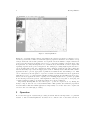
3
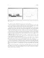
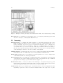
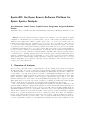
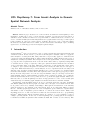
Figure 1: Screenshot showing Spot windows with imported dxf line representation, and two
examples of positioning isovists.
object called isopol). Then the constructor iterates through all the ‘walls’ of the Environment
object (enviro) and subtracts their shadow areas from its polygonal area. The resulting Area
object is the polygonal boundary of the isovist.
A number of calculations can also be performed in these isovists; a particularly interesting
one is the difference between the point from which it is calculated and the centroid of its area.
This shows a certain directionality of the space from where it is being perceived, which seems to
intuitively relate to a certain directionality feeling of that space. More in depth studies on how
this measure may relate to actual empirical data needs to be done, but at this stage it suggests
a possible interesting measure, combined with other geometrical properties of isovists.
The interface is based on windows with four menus: file, edit, view, and help. Under file
is the open and store functions. Under edit is the operative commands, add and delete isovist,
delete all, and the layer manager. In the layer manager it is possible to create and delete a layer
and assign colours to the set of isovists within the layer. Layers can also be turned on and off.
Under the view menu it is possible to choose which information to view in the work area. Graph
features can be turned on and off. Under the help menu is this paper to be found. When creating
the graphs in SPOT, one can move around, delete, or add positions and see the graphs change
in real-time.
The main function of the program is to import line drawings and position isovists within the
line drawing. The isovists are positioned by using the pointer and clicking within the drawing
area. When doing this is an isovist field expanded, limited by the imported line drawing and the
drawing area box which gives an outer limit for the isovists.
The application of several isovists with different positions but with overlapping fields gives rise
to a differentiation in colour among the overlaps due to the gamma transparency. There are two
kinds of graphs produced in this version of SPOT. Intervisibility which is an overlapping isovist
fields graph, and network graph showing relative asymmetry (RA) integration. The graph of
overlapping isovist fields is very crude and is not yet possible to calculate with any space syntax
integration measure. The gamma structure of the isovist field creates a visual effect giving the
range of the graph. The range depends on the amount of layered isovists, where there are many
overlapping isovist the graph becomes darker and where its fever it becomes lighter. The graph
4
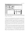
SPOT
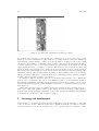
Figure 2: An example of intervisibility graph and network integration graph, generated from the
same positions.
can be said to show the visual situation created by the selected positions.
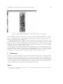
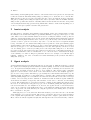
When choosing the show centroid command (figure 3) is an arrow within the isovist lit. The
arrow goes from the isovist’s starting point to the centre of the isovist. This feature is added
only for further evaluation and is not backed up with any systematic studies.
All graphs are related to layers that can be turned on and off. Each isovist position carries
information about its relation with other isovist positions. When using the show graph command,
a visibility network between the isovist positions is secleted. Each node of the network shows an
RA (relative asymmetry) value and a circle; the size of the circle depends on the RA value.
There is also a line shown between those positions seeing each other (figure 3). The thickness
of the line indicates the distance between the positions, following a ten grade scale depending
upon the size of the line drawing. The RA describes the integration of a node by a value between
or equal to 0 and 1, where all low values describe high interactions. RA is calculated by the
formula RA = 2(M D − 1)/(k − 2).
When using the move isovist command, it is possible to click and drag the isovist to any
position in the drawing area. The isovist, centroid, and network graph changes in real-time and
along the transportation between the positions.
The isovists can be divided into different sets that can be put in different layers. All layers
have an assigned color that is also seen on the isovists. Each layer can be turned on and off.
When a layer is turned on its set of isovists automatically becomes a part of the graph.
Drawing interchange format (DXF) is the only drawing format importable. The DXF format
is a tagged data representation of all the information contained in an AutoCAD drawing file.
Tagged data means that each data element in the file is preceded by an integer number that is
called a group code. A group code’s value indicates what type of data element follows. Virtually
all user-specified information in a drawing file can be represented in DXF format (Autodesk,
2006).
The program was built during a one-month period and finished during the production of this
paper. There are some minor bugs regarding importing and exporting data and sometimes in
the order of appearance of the layers and graphs; however, it works for academic use and will be
available when this paper is published.
H. Markhede, P. Miranda Carranza
5
Figure 3: Examples of integration graph and intervisibility graph, using different positions. The
arrows in the left picture are centroids.
3
Use and future development
SPOT creates a possibility to examine the dynamics between the occupied space and the occupiable space as well as dynamics between organizational relations and spatial relations. The graphs
made in SPOT can be correlated to data sets and show user patterns related to these dynamics.
Future research at SAD (Spatial Analysis and Design) aims to evaluate SPOT through using
data sets from earlier studies of office buildings made within our research group. So far, we
only looked into open plan offices and department stores. The testing of different kinds of office
layouts is crucial to prove the usefulness of the software.
Because this version of SPOT is an evaluation prototype, it has many bugs and lacks graphs
and features that could make it even more useful. The development of SPOT will primarily
handle these bugs as well as develop new graphs and measures. There are mainly three features
to focus on: to implement integration measures to the isovist field graph; to implement fixed
metric distance to the visibility integration network graph; and to make the line drawing editable
in a real-time sketching process.
To implement integration measure to the isovist field graph would make it possible to create
simplified VGA graphs. This would make it possible to compare different sub-sets of distribution
in space with the super set of the total distributed space. This would open up a process of matching the occupiabel to the occupied, and use the layer manager for testing different combinations
and solutions. A similar but different operation is local in global measure, a measure that is
common in both researchers and practitioner’s analysis. By multiplying the local measure into
the global measure, one can create graphs handling spatial phenomena originating from different
scales. This way of measuring has been successfully used when analyzing pedestrian movement
in offices (Grajewski, 1993) and movement in cities (Spacescape, 2007). In this cases were axial
line maps used for correlations. Such measure could be automatically generated in SPOT.
In addition, it would be useful to develop a visibility network node graph to calculate both
integration measures and use fixed metric measures, which have succecfully been used in other
programs (Ståhle et al., 2005). We could then investigate small differences in for example offices.
When analyzing face-to-face interactions, one could consider behavior related to the range of
6
SPOT
human performance, for example such as Hall’s (1966) social distances.
The possibility to move isovists already exists in SPOT. This feature gives a possibility to
experiment in real-time to test different solutions. We aim to develop the possibility to edit
the line drawing in real-time. This feature would have a pedagogic value and be useful for the
practitioner when evaluating small changes in their design. The tool would be able to design
both the occupied and the occupiable at the same time, or ‘designing fields directly’ as Benedikt
puts it in his classic paper (1979).
References
Autodesk, 2006. DXF Reference.
Available online http://images.autodesk.com/adsk/files/acad_dxf.pdf
Benedikt, M. L., 1979. To take hold of space: Isovists and isovist fields. Environment and Planning B:
Planning and Design 6 (1), 47–65.
Grajewski, T., 1993. The SAS head office — spatial configuration and interaction patterns. Nordisk
Arkitekturforskning 2, 63–74.
Hall, E. T., 1966. The Hidden Dimension. Anchor, New York.
Spacescape, 2007. Slussensbetydelse för stadslivet. Appendix to plan changes, Markkontoret Stockholm
stad.
Ståhle, A., Marcus, L., Karlström, A., 2005. ‘Place syntax: Geographic accessibility with axial lines
in GIS’. In: van Nes, A. (Ed.), Proceedings of the 5th International Symposium on Space Syntax.
TU Delft, Delft, Netherlands, pp. 131–143.
Turner, A., 2004. Visibility Graph Analysis. UCL, London.
Available online http://www.vr.ucl.ac.uk/research/vga/
Turner, A., Penn, A., 1999. ‘Making isovists syntatic: Isovist integration analysis’. In: de Holanda,
F. (Ed.), Proceedings of the 2nd International Symposium on Space Syntax. Vol. 3. Universidade de
Brasilia, Brasilia, Brazil.
WebmapAtHome
Nick Sheep Dalton
Department of Computing, Open University, Milton Keynes, UK
Abstract. This note describes WebmapAthome, a second-generation axial only space syntax analysis
tool, that is freely available to the wider research urban and building, design and analysis community.
This note covers some of the functionality provide with the package and discusses the rationale behind
the choice of stand alone pure axial editor over integration with other applications.
1
Introduction
WebmapAthome began as a variation of the popular Webmap application. Webmap (Dalton,
2002) was designed to be a one line axial mapping service like Hotmail or Gmail except for
the creation and processing of axial maps. While popular with students and interested parties problems arose for those who wished to use Webmap while not connected to the Internet.
WebmapAtHome takes the proven computational engine and interface then builds a standalone
application around it. This application has been the basis for some computational research and
as such has capabilities in excess of those found on the online version.
Versions of WebmapAthome including documentation can be downloaded from
http://www.thepurehands.org/webmapathome/ (User ID UAS, Password syntax05)
or
http://www.skate.bartlett.ucl.ac.uk/ (free account needed)
2
Aims and objectives
In many ways Webmap and WebmapAtHome were intended to be third generation axial mapping
software moving beyond, while being compatible with, second generation axial mapping tools
— principally Axman (Dalton, 1988). WebmapAthome aimed at those who are novices both to
space syntax and to urban and building computing in general. As such the program extends
the paradigms and functionality of programs like Axman. The principle aim was to expand on
the standalone nature of Axman by incorporating some of the peripheral supporting programs
such as JamesChoice (Dalton, 1994). At its core WebmapAthome differentiates itself from other
axial and segmental analysis programs by being largely self-contained. This emerged from the
pedagogical aim of having an application usable by those with some basic familiarity with basic
vector drawing programmes and could be used with minimal support and training in a more
academic context.
To promote the sharing of information, to aide general verification of space syntax and be a
resource new to space syntax and space syntax techniques it was felt that the software should
not depend upon other software. For example it would require less initial programmatic effort to
produce a filter or a plugin to CAD or GIS software but it was felt that many schools of architecture would not have GIS software and this would require explorative users to invest heavily in
the purchase and training to use a ‘powerful’ CAD or GIS package like Microstation or ArcInfo.
8
WebmapAtHome
Figure 1: WebmapAtHome
While use of external editing software can facilitate the rapid development of software for a researcher’s personal use, it has been found through long experience that there are a number of long
term problems associated with ‘parasitic’ development. From the human computer interaction
point of view the users are frequently expected to be competent or highly competent users of the
host platform. Secondly the integration of tool with the host environment becomes complex and
requiring expertise at the point of integration. For example processing might require the user to
export and then import into the computation engine. If this does happen it is quite possible the
user inadvertently reprocesses an inappropriate version. Thirdly most CAD and GIS software
applications fail to provide appropriate sophisticated statistical and data mining tools. This
can be remedied by the integration of yet more software but this makes the whole application
unwieldy for novice or occasional users. Finally parasitic applications can suffer from host creep,
that is, the host applications tend to rapidly evolve making plugins and cooperative programs
from following versions inoperable. WebmapAthome takes the proven path of developing self
contained software leading to an application than can be freely exchanged.
Importantly WebmapAthome does take steps to operate in ‘expert mode’ by offering the
ability to import data via vector based DXF transfer. This permits data axial line preparation
in such as GIS, CAD and CAAD applications. Importantly once in the data can be repaired as
errors are uncovered through processing.
3
Operation
To broaden the appeal of syntactical processing it was felt that it was important to be platform
neutral, to this end WebmapAthome is written in a common form of Java that can run on
N. S. Dalton
9
many platforms capable of running the JavaRunime. For many target users the Java runtime is
preinstalled and, if not, it can be easily down loaded from the Java website. This means that
the whole interface and operational design had to be interoperable on both Mac / Unix and
Windows / PC. This has a secondary benefit of insulating the user from problems caused by
operating system upgrades.
4
Information exchange
It has already been mentioned above that WebmapAthome can import DXF, but this is not
the only form of information exchange. WebmapAthome can also import binary Axman Maps
so permitting access to a large database of historic axial maps. This has the secondary benefit
that the values of the standard syntactical calculations have been checked on a like for like
basis. To provide maximum functionality axial lines can also be imported as end coordinate
pairs suitable for export from generative applications or GIS systems. Once imported the maps
can be automatically rotated (to allow for coordinate system changes) centred and scaled to fit
the publishing coordinates used.
WebmapAthome can also export in a number of formats including graph (network) formats.DOT (Koutsofios and North, 1993) and Pajek (de Nooy et al., 2005) and can also produce
vector images for both print and the internet in .SVG and .EPS formats. Exchange with programs like Depthmap (Turner, 2001) and GIS is encouraged via the ablity to export unlinks in a
number of formats. WebmapAthome’s new .AXIL (Dalton, 2003) format is both well documented
and text based permitting a number of translators to be written to new applications.
5
Editing
Combined with the ability to import both .JPEG and .GIF image formats WebmapAthome
operates in a familiar way to Axman users. Lines can be drawn / moved / edited and deleted.
For design based project this creates an unmatched fluidity of process. WebmapAthome replaces
the use of the traditional ‘bridge’ typically used to link separate floors with a new mechanism
known as a ‘super-link’: a super link is a form of inverse unlink. This selection of two separate
and non connecting axial lines enables the superlink menu which allows the user to glue the lines
together via a guide line. Superlinks automatically update when moving entire floors. For very
large axial maps an overview or navigational panel is permanently visible permitting the user to
assess their location in the larger area when zoomed in.
6
Visibility links and visibility depth, accessibility and signage
in buildings
One common problem with most axial mapping is the situation where there is an ambiguity
between visible accessibility and physical accessibility. For example a busy traffic junction where
pedestrian movement is blocked by safety fencing, or more commonly in a building with an
atrium where one can see a room on an upper floor but not directly walk there. WebmapAthome
introduces the concept of a visibility link, a link like a super link (described above) where two
spaces (axial lines) are connected by mutual visibility. By using the make visibility link it is
possible to create a second network of connections. The compute visibility depth requires an
empirical ’blend’ factor and from this creates a new type of integration that incorporates visibility
and accessibility into the syntactical representation. By introducing one way visibility links it is
10
WebmapAtHome
also possible to represent signage and so provides a method to investigate the world of signage
and way finding in a rigours syntactical setting.
7
Observations
WebmapAthome supports several ‘layers’ familiar to CAD, GIS and CAAD users. In this case
multiple layers can be used to hold gate observation data. The inclusion of observation data has
two primary aims. Firstly axial maps can be exchanged and filed inclusive of their observations.
Secondly WebmapAthome provides a number of ways of automatically attributing observations
to lines. With Axman or a traditional CAD systems lines can be associated with data, if the
axial model is adjusted in light of on the ground information it becomes tedious to re-attribute
observation data to all axial line. WebmapAthome provides mechanisms useful when dealing
with both gate or moving gate observations and point observation such as break-ins or building
type.
8
Data mining
In line with Axman, WebmapAthome has a number of interactive visualisations that can be used
to help investigate data. These include an enhanced table view that permits the creation of
unlimited numbers of new data columns including the creation of random data columns for hypothesis testing. A new column calculator similar to the graphic user interface based calculators
(first seen in Statview) is also present to permit the merging of multiple columns.
The scattergram interface is now presented simultaneously with the overall axial map. Selecting an item on the scattergram will selected the item in the main editor view. This ability
to interactively select and examine data has been enhanced in a number of ways. Firstly all
views understand the concept of a measure modifier. For example if a measure colours from
blue (maximum) to red (minimum) then selecting a negative modifier (−m) will case the colour
spectrum to become inverted: red (maximum) to blue (minimum). Equally values can be the
logarithm of the value (to extenuate the low end value differences) or the square of the value (to
extenuate the high end differences). Overall fifteen measure modifiers are present that can alter
the colour maps in many sophisticated ways. This use of measure modifiers is hypothesised to
be more valuable than alternative simple two point ’S’ curve for a number of reasons. Firstly
the modifier is comparative, if two maps have the same modifier applied then the colours are
comparative. ‘S’-curve based systems must have exactly the same point values used. Secondly
and more importantly the modifiers can be used in all the data mining components such as
the scattergram, histogram. Hence it is possible to see both the axial colour scheme and the
scattergram modified to precisely the same degree enchaning visual comprehension.
Also available in the data mining panel are a new histogram (showing the distribution of
values), legend, a new intelligibly surface and a ’finger print’ of the connectivity. This is a plot of
the table of connectivities (degrees) between differing axial lines. For example if two lines have a
connectivity of three connect to lines of connectivity five then a value of two will appear between
row three and column five.
Another significant addition is the generalised use of ‘enable/disable’ inspired by Statview
(SAS Institute, 1992). This permits an area to be investigated by the temporary removal of axial
lines from the values being investigated. For example a large axial area may be mapped but the
surrounding buffer area might be ’disabled’ to permit in the differences within the core site to be
stronger. Alternatively it is possible to exclude all singly connected axial lines within a complete
map.
N. S. Dalton
9
11
Measures
As mentioned WebmapAthome computes all the standard measures (Hillier and Hanson, 1984)
(integration, integration-3, connectivity, control) in a way (for good or evil) that is directly
compatible with Axman. The constituent values (total depth, RRA, RRA3), are computed to
aide those keen to understand the process of normalisation. A number of component measures
are also present such as k = 2 and k = 3 (that is, the number of axial lines at precisely this
distance from the appropriate starting line).
10
Angular Measures
WebmapAthome also includes the ability to compute the axial angular integration (Dalton et al.,
2003). To clarify this is a separate measure from segmental angular depth (Hillier and Iida, 2005;
Turner, 2005). WebmapAthome is purely an axial (and not segmental) computational package,
so it is possible to compute a fractional angular depth based on the angle of intersection of axial
lines as mentioned in Dalton (2001). This method also seems to have an improvement in fit with
reality, but does not abandon the gains with axial methodology (such as connectivity and hence
intelligibility). To help illuminate the issue, a single line (or group of lines) can be selected and
then coloured by the depth from the origin by both angle and step depth.
11
Multiple measures
A number of new experimental measures are presented in the application. This includes multiradii, this computes all the values of integration for a range (3-10 for example) of radius values.
The multiple measures are expanded by two new radius like features Vicinity (Dalton, 2005)
and Decay. Vicinity tries to eliminate the problems of angular relativisation by using only the
closest V number of axial lines. Decay also attempts to eliminate the mathematical process of
relativisation by including all lines but reducing the importance of a lines contribution dependant
upon the geodetic distance. In practice both Decay and Vicinity are almost (but not completely)
identical to Radius based integration. The differences are likely to be a rich source of further
research.
12
Choice
Choice (Bafna, 2003) was of long-standing theoretical interest and with the growth in computing power has again emerged as an area of research (Hillier and Iida, 2005; Turner, 2005).
WebmapAtHome now repackages the old external program called JamesChoice Dalton (1994)
that computes the syntactical definition of axial choice rather than the similar sociological algorithms.
13
Parallel (hyper-speed) processing
Many modern computers including some laptops have multiple cores. WebmapAthome takes
advantage of this by providing a new multithreaded version of the standard algorithms. By
carefully crafting a new set of algorithms, WebmapAthome can halve the computation time by
taking full advantage of both processors.
12
14
WebmapAtHome
Neighbourhood (point synergy, point intelligibility)
One of the most important new algorithms embodied in WebmapAthome is the introduction of
axial point intelligibility and axial point synergy (Dalton, 2007). This research work appears to
create a measure were similar patches of space (indicated by islands of continuous colour) appear
to indicate areas of natural neighbourhood. These research algorithms are presented to permit
other researchers to access and confirm or refute the findings and expand this fascinating area.
To facilitate checking of the neighbourhood mapping WebmapAthome also provides a general
‘point’ mapping mechanism that might be explored to find some unexpected structures.
15
Axial randomisation
One problem when looking at the findings of many investigations into the structure of axial
maps is the question to what extent the findings are the product of design intent rather than
the reasonable results of the presence of axial lines at a certain density. Axial randomisation
permits a range of ‘null’ hypothesises to be tested. The axial randomisation feature produces an
axial map that has exactly the same number of axial lines with precisely the same length and
angle distribution. The resulting random axial map has the same overall axial density (the lines
lie within the same overall extent) and is guaranteed to be continuous (there is a route from
every axial line to every other axial line). By comparing the source axial map with a number of
randomised axial maps it is possible to extract out to what degree a configuration or structure
is inherent in the use of axial lines and what part is due to what might be loosely called design
intent.
16
Summary
Webmpathome is a general purpose urban and building spatial editing and analysis tool with
a number of sophisticated features for the creation, computation, analysis and investigation
of axial maps. While this software has no segmental capabilities, its self-contained nature is
ideal for new, intermediate or infrequent use as part of research or as an architectural design
tool. WebmapAthome also bridges the cap between legacy software such as Axman and fourth
generation space syntax methods.
References
Bafna, S., 2003. Space syntax: A brief introduction to its logic and analytical techniques. Environment
and Behavior 35 (1), 17–29.
Dalton, N., 1988. Axman. UCL, London.
Dalton, N., 1994. JamesChoice. UCL, London.
Dalton, N., 2001. ‘Fractional configurational analysis and a solution to the Manhattan problem’. In:
Peponis et al. (2001), pp. 26.1–26.13.
Dalton, N., 2007. ‘Configuration and neighborhood: Is place measurable?’. In: Hölscher, C., Conroy Dalton, R., Turner, A. (Eds.), Space Syntax and Spatial Cognition. Universität Bremen, Bremen, Germany.
Dalton, N., Peponis, J., Conroy Dalton, R., 2003. ‘To tame a TIGER one has to know its nature:
Extending weighted angular integration analysis to the description of GIS road-center line data for
N. S. Dalton
13
large scale urban analysis’. In: Hanson, J. (Ed.), Proceedings of the 4th International Symposium on
Space Syntax. UCL, London, UK, pp. 65.1–65.10.
Dalton, N. S., 2002. Webmap. Ovinity Ltd, London.
Dalton, N. S., 2005. ‘New measures for local fractional angular integration: Or towards general relativisation in space syntax’. In: van Nes (2005), pp. 103–115.
Dalton, N. S. C., 2003. The WebmapAtHome AXIL Format.
Available online http://www.thepurehands.org/AXILFormat.html
de Nooy, W., A., M., V., B., 2005. Exploratory Social Network Analysis with Pajek. Cambridge University
Press, Cambridge.
Hillier, B., Hanson, J., 1984. The Social Logic of Space. Cambridge University Press, Cambridge, UK.
Hillier, B., Iida, S., 2005. ‘Network effects and psychological effects: A theory of urban movement’. In:
van Nes (2005), pp. 553–564.
Koutsofios, E., North, S. C., 1993. Drawing graphs with dot. AT&T Bell Laboratories, Murray Hill, NJ.
Peponis, J., Wineman, J., Bafna, S. (Eds.), 2001. Proceedings of the 3rd International Symposium on
Space Syntax. Georgia Institute of Technology, Atlanta, Georgia.
SAS Institute, 1992. StatView. Cary, NC.
Turner, A., 2001. ‘Depthmap: a program to perform visibility graph analysis’. In: Peponis et al. (2001),
pp. 31.1–31.9.
Turner, A., 2005. ‘Could a road-centre line be an axial line in disguise?’. In: van Nes (2005), pp. 145–159.
van Nes, A. (Ed.), 2005. Proceedings of the 5th International Symposium on Space Syntax. TU Delft,
Delft, Netherlands.
14
WebmapAtHome
Confeego: Tool Set for Spatial Configuration Studies
Jorge Gil, Chris Stutz and Alain Chiaradia
Space Syntax Limited, London, UK
Abstract. Confeego is a suite of tools to understand and harness the effects of spatial configuration in
urban systems or complex buildings developed by Space Syntax Limited and is available free for academic
use. Confeego has been developed to support the various phases of a consultancy or research project and
in that sense consists of several tools that are grouped according to the type of tasks involved. These
tasks fall generally under the categories of data translation, data collection, map processing (axial, convex
and isovists), data analysis and data visualisation. Confeego is a plug-in for the MapInfo Professional
GIS running on Windows and this has several implications in the use of the software. It might not be
ideal for space syntax beginners with no GIS experience but it offers the classic space syntax tools plus
it can import results from different space syntax software and the user benefits from functionality for
querying, displaying and analysing multiple layers of information. For those who require the analysis
of large, complex systems combining a multitude of data sources and several types of analysis Confeego
provides an adequate work platform.
1
Introduction
Confeego is a suite of tools to understand and harness the effects of spatial configuration in
urban systems or complex buildings developed by Space Syntax Limited1 and is available free
for academic use2 . It covers a range of tools that are useful to projects involving the classic
space syntax analysis related to topological depth (Hillier and Hanson, 1984; Hillier, 1996) and
other tasks related to data collection, statistical analysis and visualisation. It also allows the
integration of the results from other space syntax software tools (Turner et al., 2001; Turner,
2004; Ståhle et al., 2005).
Confeego is developed as an extension to MapInfo Professional GIS (Geographic Information
System) for Microsoft Windows and requires an installed version of MapInfo 7.8 or above to run
it. It is currently used by Space Syntax Limited and its affiliate offices on consultancy Space
Syntax Limited (2007) and research projects and is also used at UCL Space Lab and by other
researchers around the world for academic research work3 . In this paper we firstly explain the
requirements and advantages of using a GIS platform. We then introduce the task groups that
Confeego provides support to and briefly describe the different tools that compose the suite. We
proceed to discuss how Confeego positions itself as a spatial configuration analysis work platform.
Finally we conclude highlighting the key benefits of Confeego and who will make the most of its
use.
2
The GIS Platform
Confeego is a plug-in for the MapInfo Professional GIS and this has several implications in the
use of the software. On one hand it assumes that the user has access to MapInfo and is versed in
such tasks as managing data tables, executing queries or creating thematic maps. On the other
16
Confeego
hand it offers the users the ability to apply the spatial analysis and display features of a GIS to
their projects. There are several benefits in using a GIS as it integrates quantitative information
with the geometric and geographic information. By using a GIS the users can:
– Import and export drawings and data in a wide variety of vector and raster file formats
– Combine information from multiple sources as it has a common geo-referenced basis
– Draw and process complex geometries and topologies
– Analyse multiple layers of information both statistically and visually
– Perform spatial queries for exploration of topological relationships
– Use very large data sets for analysis of urban areas
– Convert geo-referenced information for use in other platforms
– Define a flexible workflow combining creatively the different of tools
If users are familiar with another GIS package or do not have the need to get started in GIS
they might not feel attracted to use Confeego, as there is a financial and time cost involved
in learning MapInfo. For those users who need a GIS in their space syntax research project
Confeego is an appropriate option because it enhances a traditional GIS that does not work with
the type of data or analysis required for space syntax research.
3
The Confeego tools suite
Confeego has been developed to support the various phases of a consultancy or research project
and in that sense consists of several tools that are grouped according to the type of tasks involved.
These tasks fall generally under the categories of data translation, data collection, map processing, data analysis and data visualisation. The first group deals with the transfer of general data
from and to other applications; the second with the entry of data collected during pedestrian
observations or built environment surveys; the third with the processing of axial or convex maps
in various ways; the fourth with the statistical analysis of the results and analysis across multiple
information layers; the final group with the graphic display of the results.
Once Confeego is installed a ‘Space Syntax’ menu becomes available in MapInfo’s menu bar
from which the users can access the individual tools. The menu is organised according to the
above groups. Below is a brief description of each of the tools included in the current release of
Confeego.
3.1
Data translation
Import map data Creates the geometry from a text file containing pairs of x,y coordinates
defining points or lines, importing as well any attributes associated with these objects, for
further spatial analysis. This tool is useful as a generic importer of processed results from
other space syntax analysis software.
Import UCL Depthmap line data Imports the results of axial or segment maps processed
in UCL Depthmap (Turner, 2004).
Export UCL Depthmap unlinks Exports Confeego unlinks for use in Depthmap or any
other software that defines them as point coordinates.
J. Gil, C. Stutz, A. Chiaradia
(a)
17
(b)
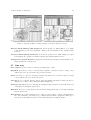
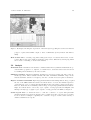
Figure 1: Typical workspace with pedestrian observation and survey maps
Import UCL Depthmap VGA Graph Imports the graph of a VGA (Turner et al., 2001)
point analysis processed in Depthmap. This is used for further isovist analysis within
Confeego.
Convert UCL Depthmap VGA Grid Converts the points from a VGA analysis processed
in Depthmap into grid tiles for further display and analysis within Confeego.
Compile Place Syntax Results Compiles the results from several Place Syntax (Ståhle et al.,
2005) analysis into a single table.
3.2
Data entry
Gate counts Prepares a table for entering pedestrian gate counts.
Snapshots Provides a toolbar for entering static snapshot observation data according to user
defined time periods, pedestrian categories and activity.
Traces Provides a toolbar for entering pedestrian following traces observation data according
to user defined time periods and categories.
Land use Tool for entering land use survey data and building information, which can then be
displayed according to three different standards (figure 1).
Frontages and fences Tool for drawing the building frontages and fences and define their level
of transparency facing the public space.
Entrances Tool for recoding entrance surveys characterising the interface between the buildings
and the public space.
Infrastructure Tool that facilitates the recording of a large variety of public realm infrastructure, street furniture, pavement types, crossings and surveillance equipment. This type of
surveys are particularly relevant for environmental impact assessment studies.
18
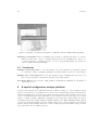
Confeego
Figure 2: Workspace showing the maps and attributes from axial, convex and isovist processing
Site photos Tool for manual geo-referencing site photos on a base map, indicating position and
direction of the photo, address plus additional notes.
3.3
Processing
Integration This tool calculates the classic measures of connectivity, integration and control
(Hillier and Hanson, 1984). It can process maps of any type of intersecting spatial object,
such as axial lines and convex polygons. In addition, integration can be calculated for
the junctions where such objects intersect. There are no built-in limits to the number of
objects that can be processed in each map, although performance will vary according to
map size and computer system specification. This tool is often used to verify the integrity
of the axial map in relation to unconnected lines or sub-systems.
Unlinks manager Tool that supports the process of creating and verifying the map unlinks these indicate that two intersecting objects cross physically at different levels.
Point depth Calculates the topological (step) or metric depth from one or more origins, based
on an axial network or a convex spaces system.
Street metrics Based on an axial map it calculates line direction, length and connectivity and
a user interface allows previewing the direction profile of the system and explore different
grid patterns according to a predominant direction (figure 3).
Block metrics This tool derives blocks from an axial map to study urban morphology and
urban grain. It calculates block size plus a series of other block shape metrics and generates
maps that display the different block patterns in the system (figure 3).
VGA isovists Given a pre-calculated grid of VGA tiles and the connections graph from UCL
Depthmap it generates a series of isovists for analysis. The isovist origin can be a point,
J. Gil, C. Stutz, A. Chiaradia
19
Figure 3: Workspace showing the exploration of urban morphology using street and block metrics
polygon or path, with similar output to that of Omnivista (Conroy Dalton and Dalton,
2001).
Real isovists This tool draws polygonal isovists given a layer of obstacles and a series of viewpoints. The isovist can be limited in distance range and a different ray tracing algorithm
can be used for building or urban environments.
3.4
Analysis
Transform data Calculates new attribute columns transformed by different mathematical operations like log, square root, squared, a constant factor, scales the values between 0 and 1
for ranking and normalises by the data set size.
Summary statistics Calculates summary statistics for the selected data sets and for the attributes specified. These statistics include like sum, maximum, minimum, range, mean,
median, standard deviation or frequency, but also correlation between pairs of attributes.
Explore statistics with JMP Exploring spatial-statistical relationships with Confeego requires
the use of the JMP statistical software but allows users to recreate the Axman experience
of selecting an object on a map and then finding its associated data point in a scatterplot.
However, users have more flexibility with Confeego in exploring spatial-statistical relationships, as it allows users to select any object capable of being represented in MapInfo and
finding it in any type of graph or plot capable of being generated in JMP; see Figure 4.
Count objects This tool allows the user to count the occurrence of objects with particular
attributes within polygonal regions that can be regular grid cells, convex spaces or isovists.
It can be used for example to quantify the occurrence of types of crime, static activity or
entrances within those regions.
20
Confeego
Figure 4: Workspace showing the integration of MapInfo with the JMP statistical package
Building to axial linker Given a buildings and an axial or segment map this tool creates a
links table that can be used to transfer attributes from the buildings layer - like socioeconomic, land use or construction data - onto the corresponding spatial objects and vice
versa for further statistical analysis.
3.5
Visualisation
Multiple ranges maps This tool produces maps of processed spatial objects (axial, segment
or convex) according to multiple quantitative measures using a selection of colour ranges.
Multiple gate count maps This tool produces maps of gates of multiple time periods according to their pedestrian count values following a user defined range.
Percentile charts Creates a series of histograms for analysing the distribution of attributes of
any spatial object.
4
A spatial configuration analysis platform
Confeego runs integrated in a GIS platform and consists of a range of tools for tasks at various
stages of a research project. As such it can be used for more than traditional space syntax related
research. It might not be ideal for space syntax beginners with no GIS experience who need to
focus on understanding the basic principles of space syntax. But it gives support at various
levels to complete spatial configuration analysis projects using space syntax methodologies in
combination with other spatial analysis techniques (Jiang et al., 2000). Running within a GIS it
becomes a work platform with no fixed workflow, many of its tools being useful beyond what is
described in the user’s manual. The more common tasks get automated with Confeego and the
rest comes with each one’s GIS experience.
J. Gil, C. Stutz, A. Chiaradia
21
Furthermore Confeego should not be seen as a competitor to other space syntax software.
It can import results from other software and the user benefits from functionality for querying,
displaying and analysing multiple layers of information.
Finally Confeego is a reflection of the way Space Syntax Limited works in consultancy projects
using MapInfo and other software programs (Space Syntax Limited, 2007), and is a principal
means of achieving efficiency and freeing up time for more exploratory endeavours. It is continuously under development to fix bugs4 and add new features or tools5 , and is tested in an
environment where the feedback loop between the users and the development team is very short.
5
Conclusion
Confeego is a suite of tools for spatial configuration analysis and that supports tasks at various
stages of a research project. These include data translation, data collection, map processing,
data analysis and data visualisation. It has been designed to run integrated within the MapInfo
GIS platform for Microsoft Windows.
It might not be the ideal tool for space syntax beginners with no GIS experience who might
prefer a simpler standalone and cross platform application6 . Nor for those who from the nature
of their research do not require any of the benefits of a GIS platform. For those who require
the analysis of large, complex systems combining a multitude of data sources and analysis types
Confeego provides an adequate work platform and offers the classic space syntax tools plus
supports tasks that go beyond traditional space syntax related research. Each user can be
creative in how the Confeego tools are applied within the GIS to address the research problems
in hand.
If users are already using MapInfo for parts of their research and other space syntax software then Confeego can be integrated into the workflow as it complements existing software by
importing the results for further spatial-statistical analysis.
Confeego was developed for consultancy and research projects at Space Syntax Limited and is
used daily and reviewed to ensure efficiency in routine tasks moving the focus onto understanding
and exploring the effects of spatial configuration in urban systems and complex buildings.
Notes
1 Confeego
was created by Chris Stutz, Jorge Gil, Eva Friedrich and Corey Klaasmeyer
register for a copy of Confeego you should visit the following URL: http://www.spacesyntax.org/register.
aspx Please note that the software is free for academic use only and we will have to verify your academic status
before we can authorise your account.
3 If you use Confeego for your research project please remember to credit it as follows: Space Syntax Limited
(2007) Confeego v2.0, London, UK
4 The software is continuously tested but is not 100% free of bugs, especially when run in new environments
and using different data sets. If you encounter any bugs in Confeego, please record the exact conditions in which
it occurred in an email message and send it to [email protected]
5 If you want to suggest new features for future versions of Confeego, please send them out in an email to the
support email address. Please note that it may not be possible to implement all suggestions.
6 Because the software is made available for free only limited technical support is available. Please refer to
the documentation provided with Confeego or email [email protected]. Space Syntax Limited
cannot offer any telephone support nor offers technical support for MapInfo Professional, JMP, or the Microsoft
Windows operating system.
2 To
22
Confeego
References
Conroy Dalton, R., Dalton, N., 2001. ‘Omnivista: An application for isovist field and path analysis’. In:
Peponis, J., Wineman, J., Bafna, S. (Eds.), Proceedings of the 3rd International Symposium on Space
Syntax. Georgia Institute of Technology, Atlanta, Georgia, pp. 25.1–25.10.
Hillier, B., 1996. Space is the Machine. Cambridge University Press, Cambridge, UK.
Hillier, B., Hanson, J., 1984. The Social Logic of Space. Cambridge University Press, Cambridge, UK.
Jiang, B., Claramunt, C., Klarqvist, B., 2000. An integration of space syntax into GIS for modelling
urban spaces. International Journal of Applied Earth Observation and Geoinformation 2, 161–171.
Space Syntax Limited, 2007. Croydon town centre: Baseline analysis of urban structure, layout and
public spaces. Croydon council local development framework (LDF), croydon metropolitan centre
area action plan (AAP), Croydon Council.
Available
online
http://www.croydon.gov.uk/planningandregeneration/planningpolicy/
localdevelopmentframeworkldf/croydonmetropolitancentreare
Ståhle, A., Marcus, L., Karlström, A., 2005. ‘Place syntax: Geographic accessibility with axial lines
in GIS’. In: van Nes, A. (Ed.), Proceedings of the 5th International Symposium on Space Syntax.
TU Delft, Delft, Netherlands, pp. 131–143.
Turner, A., 2004. Depthmap 4: A researcher’s handbook. Tech. rep., Bartlett School of Graduate Studies,
UCL, London.
Available online http://www.vr.ucl.ac.uk/depthmap/depthmap4.pdf
Turner, A., Doxa, M., O’Sullivan, D., Penn, A., 2001. From isovists to visibility graphs: a methodology
for the analysis of architectural space. Environment and Planning B: Planning and Design 28 (1),
103–121.
Syntax2D: An Open Source Software Platform for
Space Syntax Analysis
Jean Wineman, James Turner, Sophia Psarra, Sung Kwon Jung and Nicholas
Senske
Taubman College of Architecture and Urban Planning, University of Michigan, Ann Arbor, USA
Abstract. For space syntax researchers, software is an essential tool for the analysis of spatial
configuration. Unfortunately, the proprietary nature of most of this software can inhibit innovation
within the field. Without the ability to examine others’ source code, we lose a potential resource for
learning and an additional point of verification for peer review. Moreover, without a common base of
code, researchers must constantly duplicate existing efforts when developing new software. As a result
of proprietary policies, many spatial analysis programs end up limited in scope and become difficult
to maintain as their authors move on to other research. The development of space syntax is hindered
as long as software remains closed and fragmented. Towards this end, the University of Michigan has
developed an open source platform for spatial analysis: Syntax2D. This software currently features
a robust interface, combining existing measures such as isovist, graph, and axial analysis with newer
features for path analysis. Our goal is for Synax2D to become a collection point for researchers, unifying
different methods of analysis within a single application. With the software and source code freely
available, Syntax2D is an opportunity for the space syntax community to share and build upon their
work across a common framework.
1
Overview of features
Our objective of the first version of Syntax2D is to lay the framework for future development.
At this early stage, we are more interested in incorporating existing measures and establishing
a workable interface between them than in pushing the limits with new features. Therefore,
on the surface, it would seem there is not much to distinguish Syntax2D from other recent
spatial analysis programs. It meets the basic needs of space syntax research with isovists, axial
maps1 , and grid / VGA analysis. Users can import .dxf files and export data to .csv. The
interface features mouse, pan, and zoom, and visualization layers that can be toggled on and off.
Although it may not yet have the depth of features of existing programs, this version is fully
capable. Students at the University are currently using Syntax2D for their research.
One of our original contributions is the inclusion of new path-based measures. While the computer modeling techniques of spatial characteristics are being continuously refined and improved,
the representation and analysis of how people move are still carried out using manual methods.
Syntax2D quantifies traces of people paths so that these can be tested against spatial values as
well as data obtained from observation studies. Users can load a path from within a drawing
and use it to generate isovists from a series of observation points. From here, the cumulative
isovist of the path is shown and the data from each of these points is analyzed according to
several measures. Another option for this tool is to generate isovists with a user-specified cone
of vision. Syntax2D is capable of representing data visually from the point measures, as well.
24
Syntax2D
Figure 1: A path isovist visualisation showing area values
For example, the area value of each isovist can be displayed as a colored circle along a path
(figure 1). A greater radius and a red hue might denote a larger relative isovist area. Finally, we
have included a path-counting tool that can count the number of times a path crosses a VGA
cell, and a point-counting tool that will count how many points appear in each VGA cell. These
tools have already proven to be great time savers in our own research. In the future we will add
output measures related to a number of behavior characteristics, such as direction seeking and
direction change in a navigable space. Each cell is given an attribute based on such measures.
The results can be statistically processed and interfaced with data from visibility analysis. The
usefulness of this tool and its applicability in studies looking at human behavior is widely significant providing a platform for a detailed study of the relationship between syntactic variables
and the complex aggregate patterns of movement.
In addition to this set of features, there are several minor improvements of note. Within the
point isovist tool, users have the option of subdividing isovists to obtain additional measures.
Our visibility analysis automatically detects enclosed spaces and offers complete control of both
grid spacing and starting point. VGA visualizations have full color depth and display a reference
scale (figure 2).
While this is an early version, we think it shows great promise. In the long term, we hope to
improve the depth of the software with a greater variety of measures and its breadth with more
analysis types such as J-Graphs. Ultimately, we hope that researchers will find Syntax2D useful
enough that they would like to help us improve upon it.
2
Licensing and development
Syntax2D is free to download from the University of Michigan so long as users agree to the terms
of the open source license. This allows the user to install and run the program for academic
research as well as to view and modify the source code2 . Users are under no obligation to share
J. Wineman, J. Turner, S. Psarra, S. K. Jung, N. Senske
25
Figure 2: VGA analysis with full color depth and a reference scale display
any modifications they make, but cannot re-release programs containing Syntax2D code in the
form of commercial software. Papers published using software derived from any Syntax2D code
must cite the authors of the original code.
With the introduction of the software, the University will be launching a website where users
can discuss their needs and coordinate their own development efforts. This site will host the full
archive of all future revisions of Syntax2D, as well as supplemental documentation and tutorials.
In time, we hope that users will contribute to the website, both as members of an active learning
community and as co-developers of the software.
Development of the software will follow a model similar to that of Linux, whereby usersubmitted suggestions and code are vetted by a committee and then incorporated into the ”official” version of the software at regular intervals. In this manner, we hope to control the quality
and usability of the software while retaining community involvement in its evolution.
3
Conclusion
If software is a vital component of space syntax research, then its politics are as important as
its features. Proprietary academic software is a contradiction; transparency is essential if we are
to engage in peer review and build upon each other’s work. We believe that open source, which
both protects and encourages contributions, is the best policy. Therefore, we offer Syntax2D, an
open source platform for space syntax analysis, as the first step in this direction. We hope that
other programs and researchers will join us in supporting this effort.
Notes
1 Axial maps are somewhat limited in this version. Once we have them optimized, we will have the full suite
of axial tools in the next version.
26
Syntax2D
2 Currently, modifications to the source code require Microsoft Visual Studio, which is not freely available. The
decision to use Microsoft libraries was made to speed development time of the first version. We hope to eliminate
this dependency in the future.
References
Benedikt, M. L., 1979. To take hold of space: Isovists and isovist fields. Environment and Planning B:
Planning and Design 6 (1), 47–65.
Conroy Dalton, R., Dalton, N., 2001. ‘Omnivista: An application for isovist field and path analysis’. In:
Peponis et al. (2001), pp. 25.1–25.10.
Peponis, J., Wineman, J., Bafna, S. (Eds.), 2001. Proceedings of the 3rd International Symposium on
Space Syntax. Georgia Institute of Technology, Atlanta, Georgia.
Turner, A., 2001. ‘Depthmap: a program to perform visibility graph analysis’. In: Peponis et al. (2001),
pp. 31.1–31.9.
Turner, A., Doxa, M., O’Sullivan, D., Penn, A., 2001. From isovists to visibility graphs: a methodology
for the analysis of architectural space. Environment and Planning B: Planning and Design 28 (1),
103–121.
Segmen: A Programmable Application Environment
for Processing Axial Maps
Shinichi Iida
Bartlett School of Graduate Studies, UCL, London, UK
Abstract. Here I introduce Segmen, an experimental application I have developed for computing
various space syntax measures. Notable about its features are that it has an extended set of axial and
segment unlinks and vlinks, and that it can be completely programmable.
1
Introduction
Segmen is an experimental application environment which essentially does graph computation
for axial/segment maps in order to obtain various configurational measures. It has been written
entirely in Common Lisp and can be compiled and run on any platform that has a Common Lisp
implementation. For the convenience of the user, the author currently provides the compiled
images of the program on both Mac OS X and Microsoft Windows. On Mac OS X, Gary Byers’
OpenMCL (version 1.1 Alpha) (Byers, 2001) has been used to compile and generate the image,
and the user needs to set up OpenMCL environment in order to run Segmen. On Windows,
Segmen is a stand-alone application and has been compiled using Xanalys LispWorks (version
4.2) (Xanalys Corporation, 2001).
Both platforms provide only a basic user interface (figures 1 and 2). In fact, when you launch
Segmen, it simply opens a command-line interface window of the Common Lisp programming
environment similar to the Unix shell (on Mac OS X) or Command Prompt window (on Windows)
and is then ready to take Common Lisp ‘functions’ from the user. In addition to the generic
Common Lisp functions, Segmen defines its own set of functions to open the map data, build
topology among the axial lines in the map and compute configurational properties.
2
A typical session in Segmen
The user interacts with Segmen by typing Common Lisp functions in the window. The following
sequence of functions is the operation the user takes in a typical analysis of an axial/segment
map:
Listing 1: The basic series of functions typical in Segmen
(open-table :mif t :file Barnsbury.MIF :depthmap t)
(read-unlink-data :file Barnsbury_unlink.txt)
(build-topology :remove-ends t :leave-if-longer-than-percent 25)
(calc-sys2 :weight ’traditional :radius 3)
(calc-choice2 :weight ’traditional :radius ’(3 t))
(calc-sys2 :weight ’simple :radius 4 :rad-mode ’route-length)
(calc-choice2 :weight ’simple :radius ’(4 8 12 16 24 32 t)
:rad-mode ’route-length)
28
Segmen
Figure 1: Segmen in operation on Mac OS X upon launching
Figure 2: Segmen in operation on Windows upon launching
S. Iida
29
(write-data :mif t :axial Barnsbury_ax.MIF
:segment Barnsbury_seg.MIF)
Each function in the above sequence does a clearly-defined task which corresponds to the
respective verbal description shown below:
1. Open the axial map from Barnsbury.MIF (in MapInfo MIF). Emulate Depthmap in assigning ID to the axial lines and segments.
2. Read the text file Barnsbury unlink.txt to register unlinks.
3. Build topology of the axial map and create a segment map. Ignore any segment stubs that
are shorter than 25 per cent of the original axial lines.
4. Calculate configurational values of the axial map. Use Radius 3 as the local measure.
5. Calculate choice-related measures of the axial map. Calculate Radius n and 3.
6. Calculate configurational values of the segment map using the angular analysis. Use Radius
400 metric distance units as the local measure.
7. Calculate choice-related measures of the segment map using the angular analysis. Calculate
Radius 400, 800, 1200, 1600, 2400, 3200 and n metric distance units.
8. Save the results in MapInfo MIF. Save the axial data as Barnsbury ax.MIF and the segment
data as Barnsbury seg.MIF.
There are many more functions and options available. The Segmen Reference Manual 1 explains what they do and how to use them.
3
Unlinks, vlinks and exclusions
One of the features of Segmen is that it takes a more comprehensive approach in defining unlinks
and links which may not be derived geometrically. To this end it distinguishes three different
properties for both axial and segment analyses: unlinks, vlinks and exclusions.
Unlinks are intersections between lines which are adjacent to each other on the plan but
are not considered as neighbours. Essentially this means to instruct Segmen to prohibit from
considering the movement from line A to line B and/or the movement from B to A despite the
fact that the two look connected. Axial and segment unlinks are maintained separately, but the
effect of axial unlinks naturally spills into the generation of the segment maps (which means the
axial unlinks must be applied before building topology), whereas segment unlinks only affect the
topology of segment map.
Virtual links (‘vlinks’) are those which connect two axial lines/segments that do not have a
natural direct connection. Once connected, they provide a one-way/two-way connection between
those elements, but they are represented internally quite differently from normal links. Segment
vlinks are set up so that they can be accessed regardless of the direction which the route is being
made in the linking segments; conceptually, the vlink is located in the middle of the segment,
and it can be used from both directions of the originating segment and it can go to any one of
two directions that are available in the destination segment. Segment vlinks are also reflected
in the axial vlinks, but if axial vlinks are added manually, they will not be reflected in segment
vlinks. In general, axial vlinks can be considered as truly virtual existence, and their locations
are absolutely undefined. It is also true that vlinks are not naturally associated with any of
30
Segmen
the ‘weighting’ modes that have certain implications on the physical arrangement of origins and
destinations, so the user needs to provide one(s) when defining a vlink. Unlike other structural
elements, each vlink can hold unspecified number of different weights, and you can even give
the weight a name which is not one of the pre-defined 2 weight names. A non-pre-defined weight
name, such as experiment1, would work as a group name and it can be specified when depthand/or choice-related measures are calculated.
Exclusions mark the axial lines/segments which are not to be involved in the process of
calculating any configurational measures. The excluded axial lines/segments will not be an
origin or destination, nor will they be part of any shortest path found in the system. When an
axial exclusion is registered, all the segments that originally belong to that axial line are also
excluded. However the axial exclusion does not invoke rebuilding the topology of the segment
map. The exclusions have been designed not to alter the topology of the entire maps, so the
segments which have been divided by the excluded line remain divided.
An example of using both exclusions and unlinks might be to implement road traffic management on a segment map. Setting one-way roads or banned sections can be done by excluding
segments in one/both direction(s), and making segment unlinks between neighbouring segments
can be regarded as imposing turn restrictions.
4
Programmability in Segmen
Another feature of Segmen is that it is entirely programmable by the user so that the behaviour
of the application can be controlled and modified, or even a new measure can be introduced.
Since the application includes the full Common Lisp environment, the user can define her own
functions in Segmen and compile and run them immediately. Unlike other scripting languages,
the compiled user functions in Segmen are native to the operating system and therefore run at
the same speed as other Common Lisp functions.
For example, you could define a new function called my-batch-process which executes the
sequence of functions shown earlier in this paper automatically. A generic Common Lisp special
form defun can be used and the definition might look like:
Listing 2: Definition of my-batch-process
(defun my-batch-process ()
(open-table :mif t :file Barnsbury.MIF :depthmap t)
(read-unlink-data :file Barnsbury_unlink.txt)
(build-topology :remove-ends t :leave-if-longer-than-percent 25)
(calc-sys2 :weight ’traditional :radius 3)
(calc-choice2 :weight ’traditional :radius ’(3 t))
(calc-sys2 :weight ’simple :radius 4 :rad-mode ’route-length)
(calc-choice2 :weight ’simple :radius ’(4 8 12 16 24 32 t)
:rad-mode ’route-length)
(write-data :mif t :axial Barnsbury_ax.MIF
:segment Barnsbury_seg.MIF))
Once the function has been defined, simply typing:
(my-batch-process)
will do the sequence of operations from start to end.
The function can be made more generic by letting values of keywords used above be passed
as arguments:
S. Iida
31
Listing 3: Definition of my-batch-process2
(defun my-batch-process2 (input-filename ax-output-filename seg-output-filename
unlink-filename
ax-radius-depth ax-radius-choice
seg-weight seg-radius-depth
seg-radius-choice seg-rad-mode)
(open-table :mif t :file input-filename :depthmap t)
(read-unlink-data :file unlink-filename)
(build-topology :remove-ends t :leave-if-longer-than-percent 25)
(calc-sys2 :weight ’traditional :radius ax-radius-depth)
(calc-choice2 :weight ’traditional :radius ax-radius-choice)
(calc-sys2 :weight seg-weight :radius seg-radius-depth
:rad-mode seg-rad-mode)
(calc-choice2 :weight seg-weight :radius seg-radius-choice
:rad-mode seg-rad-mode)
(write-data :mif t :axial ax-output-filename
:segment seg-output-filename))
Then typing:
(my-batch-process2 Barnsbury.MIF Barnsbury_ax.MIF Barnsbury_seg.MIF
Barnsbury_unlink.txt
3 ’(3 t) ’simple 4 ’(4 8 12 16 24 32 t) ’route-length)
produces the same result as my-batch-process, but with more flexibility.
Even the existing functions can be overriden by re-defining them this way. For example,
d-value can be re-defined to calculate relative asymmetry of the corner vertex of a regular grid
with n vertices (see Krüger, 1989, for more information on this value), which is given as:
√
2(n n − 2n + 1)
Gn =
(n − 1)(n − 2)
Normally, the d-value of n = 3 and n = 22 will be as follows:
? (d-value 3)
0.21089661
? (d-value 22)
0.21428572
Typing the following function definition in Segmen will override the existing definition and let
d-value to compute Gn instead:
Listing 4: Overriding the definition of built-in d-value
(defun d-value (n)
(/ (* 2 (+ (- (* n (sqrt n))
(* 2 n))
1))
(* (- n 1)
(- n 2))))
Now if you issue d-value:
? (d-value 3)
0.19615221
? (d-value 22)
0.28661498
32
Segmen
and write-data will produce integration values using a new definition of d-value.
Following is a further example of the Common Lisp code which implements the user’s own
version of functions that calculate total depth of the axial lines.
Listing 5: Alternative definition for calculating total depth
\footnotesize
\begin{verbatim}
;;; this is an example shown in the Segmen Reference Manual
;;;
;;; my-bfs-sub is called from within my-bfs and it has 4 arguments:
;;; - id-list
A list of axial ID which are (current-depth);;;
steps away from the root space.
;;; - done-id-list
A list of axial ID which have already been inspected.
;;; - current-depth
The axial lines in id-list have this depth.
;;; - total-depth-acc An accumulator for counting total depth.
;;;
(defun my-bfs-sub (id-list done-id-list current-depth total-depth-acc)
(if (null id-list)
total-depth-acc
(my-bfs-sub (remove-if #’(lambda (x)
(or (member x id-list)
(member x done-id-list)))
(remove-duplicates
(reduce #’append
id-list
:key #’(lambda (v)
(axline-neighbors
(find-axline-id v))))))
(append id-list done-id-list)
(+ current-depth 1)
(+ total-depth-acc
(* (length id-list)
current-depth)))))
;;; my-bfs scans all axial lines from the line ID: id and returns
;;; its total depth.
(defun my-bfs (id)
(my-bfs-sub (axline-neighbors
(find-axline-id id))
(list id)
1
0))
;;;
;;;
;;;
;;;
my-calc-sys computes total depth and registers the value in
the data structure for the axial lines whose ID are between
start and end. Note that the total depth is stored in the slot
of the structure in the form of an array.
(defun my-calc-sys (start end)
(let ((start-id (get-id-by-userid-ax start))
(end-id (get-id-by-userid-ax end))
S. Iida
33
(counter 0))
(do* ((id start-id (+ id 1))
(axline (find-axline-id id)
(find-axline-id id)))
((or (null axline)
(> id end-id))
counter)
(incf counter)
(setf (axline-totaldepth axline)
(vector (my-bfs id)))
(when (zerop (mod counter 10))
(print counter)))))
\end{verbatim}
Typing:
(my-calc-sys 1 100)
is roughly equivalent to running:
(calc-sys2 :weight ’traditional :radius ’(t) :start 1 :end 100)
although it runs slower and calculates only total depth.
5
Acknowledgements
The author would like to thank the following people: Professor Bill Hillier and Professor Alan
Penn (UCL) for their kind and continuous support and advice for the author’s project; Nick
Dalton (UCL) for his products Axman (Dalton, 1988) and Ovation (Dalton, 2001) which inspired
the author to develop the software; Alasdair Turner (UCL) for his amazing programming effort
for Depthmap (Turner, 2000, 2001), which kindly incorporates many of the measures and models
that have been gradually developed through this program; Professor Yasushi Asami (University of
Tokyo) and Professor Ayşe Sema Kubat (ITU) for having given to the author the first opportunity
to apply segment computation to the real project; my colleagues at UCL and Space Syntax
Limited and Kerstin Sailer (TU Dresden/UCL) for kindly trying and testing the software.
Notes
1 Available
2 Curently,
from the author or online.
pre-defined weight names are: traditional, simple, vector, constant, constant2 and metric
References
Byers, G., 2001. OpenMCL, Version 1.1-Alpha. Clozure Associates, Somerville, MA.
Available online http://openmcl.clozure.com/
Dalton, N., 1988. Axman, Version 3. UCL, London, electronically available through Space Syntax Limited.
Dalton, N., 2001. Ovation, Version 1.6.3. Ovinity Ltd, London, electronically available through Space
Syntax Limited.
34
Segmen
Krüger, M. J. T., 1989. On node and axial maps, distance measures and related topics, paper for the
European Conference on the Representation and Management of Urban Change, Cambridge, 28–29
September 1989.
Turner, A., 2000. Depthmap, Version 7. UCL, London, available electronically through Space Syntax
Limited.
Turner, A., 2001. ‘Depthmap: a program to perform visibility graph analysis’. In: Proceedings of the
Third International Space Syntax Symposium. Georgia Institute of Technology, Atlanta, GA, pp. 31.1–
31.9.
Xanalys Corporation, 2001. LispWorks, Version 4.2. LispWorks Ltd, Cambridge, UK.
Place Syntax Tool — GIS Software for Analysing
Geographic Accessibility with Axial Lines
Alexander Ståhle† , Lars Marcus† and Anders Karlström‡
†
‡
School of Architecture, KTH, Stockholm, Sweden
Department of Infrastructure, KTH, Stockholm, Sweden
Abstract. The Place Syntax Tool (PST) is a plugin application for the desktop software MapInfo
written in MapBasic and C/C++. The plugin was developed since conventional accessibility research
and space syntax research face an almost symmetrical problem when it comes to analysing and predicting urban pedestrian movement. In this paper we explore the possibilities to combine the space
syntax description of the cognitive environment, i.e. topological axial line distance, with conventional
descriptions of attraction into a combined accessibility analysis model that we call ‘place syntax’. The
model is tested with a new GIS-tool for MapInfo called the Place Syntax Tool.
Pedestrian movement was observed in two urban areas in Stockholm; the ‘premodernist grid morphology’ Södermalm and the ‘modernist tree-like morphology’ Högdalen. We can conclude that the place
syntax model, when calculating accessibility to population or floor area measured within axial lines,
post-dicts pedestrian movement at the same high level as conventional axial line integration analysis in
the case of Södermalm, but considerably better in the case of Högdalen. Compared to ordinary metric
accessibility analysis by straight line or walking distance to population density place syntax is better in
both cases. Based on these initial findings and theoretical investigations we believe that the place syntax
approach have great potential for detailed spatial analysis and accessibility research at large, but also
for practical urban planning and design.
1
Introduction: integrating space syntax and accessibility research
For a long time accessibility research of human behaviour was limited by the kind of data and
analytical tools available. For example ‘there was no effective means for representing or dealing
with the spatial complexity of a realistic urban environment’, neither did past studies ‘incorporate
data about a person’s cognitive environment into the analytical framework’ (Kwan, 2000). In
the past decade many steps have been taken to overcome these limitations, for example, ‘instead
of using the straight-line distance between two locations, the actual travel distance over the
transportation network can be used’ (Kwan, 2000). Kwan et al. (2003) state that still much
remains and especially the understanding of our cognitive environment is pointed out to be a
crucial issue.
Accessibility is a widely used spatial analytic measure defined as the relative ‘proximity’ of
one place i to other places j. In generalised terms, the measure can be defined as:
Ai
=
X
f (Wj , dij )
(1)
where Wj is some index of the attraction of j and dij is a measure of impedance, typically
the distance of travel time of moving from i to j (Jiang and Claramunt, 2000). From this
36
Place Syntax Tool
definition it is easy to see how space syntax does not deal with the full concept of accessibility,
in that one rarely deal with Wj or any indexes of place attraction. Another way of putting
it is that accessibility research deals with ‘places’, where ‘place’ simply means a geographically
specific space, a location, or a space with a specific content, while space syntax only deals with
‘spaces’, i.e., spaces or locations with no specified content and thereby no measurable attractivity.
This straightforward distinction, between space and place, can be said to be the basis of what
Jiang and Claramunt (2000) distinguish as ‘geographic’ and ‘geometric’ accessibility1 . Hence, if
geographic accessibility is the proximity of places, then geometric accessibility is the proximity
of spaces, i.e. setting Wj = 1. Geometric accessibility can be defined as:
Ai =
X
Aij =
X
f (dij )
(2)
From this Jiang and Claramunt (2000) have shown why space syntax from the point of view
of accessibility research is a special case of geometric accessibility.
Defining how to measure dij , the ‘distance’, ‘transport cost’ or ‘energy effort to move’ from i
to j, is then obviously a critical part of a accessibility measure, and in a geometric accessibility
measure the critical part. The most common distance units used within accessibility research are:
topological steps in a network, Euclidian metric distance, travel time, travel cost and monetary
charges. But it is exactly concerning such descriptions and measurements of distance one have
encountered problems within accessibility research when moving from the comprehensive level
of geography to the detailed level of urban settings: ‘what is dramatically absent are tools
for developing accessibility measures at fine spatial scales which involve the geometry of urban
structure in terms of streets and buildings in contrast to the measurement of accessibility at the
geographic or thematic level’ (Jiang and Claramunt, 2000).
We then also see that it is here the morphological descriptions developed within space syntax
can prove useful and can contribute to accessibility research.
2
Place syntax: geographic accessibility with axial lines
We now seem able to set up an almost symmetric problem. On the one hand we have accessibility
research and urban morphology in general where one lack of experiential descriptions of urban
form. On the other hand we have space syntax where one has problems integrating place data
in certain urban areas for, e.g. predicting movement2 . Thus it seems very natural to try axial
descriptions as a measurement of distance within geographic accessibility. On the one hand
this would mean a possibility to ’load’ geographical data for improved predictions of pedestrian
movement within space syntax. On the other hand, and more interestingly, this would mean an
improved tool for accessibility analysis in general; the linear, rather than for example the metric,
accessibility to any asset or service we find in a city. It is exactly such a tool we have developed
as an extension to the GIS software Mapinfo and given the name the Place Syntax Tool3 .
From the perspective of space syntax, in place syntax we mean to put back attraction of Wj
into the geometric accessibility formula (equation 2). And from geographic accessibility formula
(equation 1) we want to put the axial line into dij :
dij
m m m
z
= h(Γ(xm
ij , yij , tij , eij , . . .), Θ )
(3)
where, Γ(·) is a representation of space, and Θz is a vector characterizing the preferences
of individuals. The representation of physical space may utilize many different variables. For
m
m
instance, xm
ij is walk distance and yij is bird’s flight distance both by mode in meters, tij is travel
A. Ståhle, L. Marcus, A. Karlström
37
Figure 1: Software structure of the Place Syntax Tool.
time by mode, and em
ij is the number of axial steps by mode m. The full place syntax formula,
a ‘geographic accessibility measure with axial lines’ then looks like this.
Ai
=
X
z
f (g(Wj , Θa ), h(Γ(em
ij ), Θ ))
(4)
This formula is the major task for the Place Syntax Tool. The tool however also manages to
m
m
m
calculate xm
ij and yij , respectively, and also a combination of eij and xij .
3
The Place Syntax Tool
Together with a group of students at the Department of Numerical Analysis and Computer Science at KTH4 , we have developed the Place Syntax Tool (PST), an application for the desktop
software MapInfo5 . The PST consists of two main components, MapBasic (MB) and Dynamic
Link Library (DLL). The MB component is written in MapBasic and implements reading and
writing in MapInfo’s own databases. The DLL component is written in C/C++ and is compilated as a DLL. It takes care of the graphical user interface (GUI) and does the accessibility
calculations. The two communicate through a communication interface integrated within the
DLL.
The GUI has two main windows. In the first window all tables are selected: input place data
(plots or address points) and output place data (where the results will be distributed: plots or
address points), axial lines and ‘unlinks’ (points where crossing axial lines do not connect), links
(e.g. address points which link plots to closest axial line).
The second window is for selecting type of analysis and consists of five pages. In the ‘Calculation type setting’ page you can choose to calculate from all places or just from a single place. In
the ’Criteria settings’ page the column for desirable place data is selected. Here you can choose
multiple columns. Data can also be normalized and given a relative weight. In the ‘Result settings’ page you choose how results are displayed, in a table or on a coloured map in MapInfo.
Here there is also a critical section where you on the one hand decide how data on input place
data are distributed to the address points, divided with the amount of address points or the full
38
Place Syntax Tool
Figure 2: Window 1 (left) and window 2 (right) in the Place Syntax Tool.
value to all. Similar to that, the output place data has to be determined, whether they are to
collect the mean, max or min of the result values at the address points (that is if you do not
choose to display them on the address points). In the ‘Table Column Keys’ page you select the
key columns that connect, e.g. address points and plots.
4
Empirical test: set-up
The first thing we wanted to examine was if accessibility to population or built floor area,
measured metrically or with axial lines, would correlate with observed pedestrian movement and
if so how it would compare with the integration analysis. The two urban areas already presented,
Södermalm and Högdalen, were once again used6 . They are delimited for maximum convexity
and so that their size is 100 hectares each. Axial maps with buffer zones were constructed for
the two areas where the deformed grid of Sdermalm turned out to have a mean axial line length
of 221 meters and consist of 131 axial lines, while the interrupted grid of Högdalen had a mean
axial line length of 100 meters and consisted of 435 axial lines. Observations of pedestrian flows
were conducted at 28 gates in Södermalm and 41 gates in Högdalen during two days (one rainy
and one sunny), at five different times during both days, each lasting five minutes. In this way
each gate was observed 50 minutes in total7 .
Four types of accessibility analyses with ten different radii (dij ) were executed with PST:
accessibility to population8 measured with axial lines, floor area with axial lines, population
with walk distance, population with bird’s flight distance9 . The analyses where also tested with
two different radii of the buffer area: 700 meter and 2500 meter (both birds’ flight distance). The
latter was based on the general rule of approximately 30 minutes walk distance10 around a study
area, often used within space syntax. Correlations between the observed flow (logarithmic) and
the accessibility analyses using PST, as well as integration analyses using Webmap, were then
compared.
5
Empirical test: findings
The main findings in our empirical test are basically of three types.
A. Ståhle, L. Marcus, A. Karlström
39
Figure 3: Map of accessibility to population r-3 Södermalm-area (0 − 60 000 persons) and r-6 for
the Högdalen-area (0 − 11 000 persons). Maps are not comparable in terms of colour (darker is
higher ‘configurative’ population).
5.1
Pedestrian movement prediction
We can conclude that PST, when calculating accessibility to population or floor area measured
with axial lines, predicts pedestrian movement at the same level as an integration analysis in
the ‘deformed grid’ of Sdermalm, but, more interestingly, considerably better than integration
analysis in the ‘interrupted grid’ of Hgdalen. The apparent reason is that PST captures the
heterogeneous distribution of population densities in and around Hgdalen. Even though the
correlations are lower in Hgdalen all over the line than in Sdermalm, the R2-value 0.4417 for
PST (axial, pop, radius-6) must be considered fair. The variations in correlation using the
different measurements are however interesting in themselves, and probably tell us something
fundamental about the planning paradigms used in the two areas.
Furthermore, since calculations with PST are based on absolute numbers of population a coefficient can be derived by dividing the observed movement-values with the place syntax value. This
‘movement production coefficient’ can then be used to predict movement in places not observed,
in absolute numbers, not only relatively as in the integration analysis. Taking the measures with
the best correlations, the axial population configuration r3-coefficient for Sdermalm is 0.013 and
the axial population configuration r6-coefficient for Hgdalen is 0.026.
5.2
Distance measures
We can conclude and confirm that the axial line is superior to any metric distance measure,
walk or bird’s distance, especially in the ‘deformed grid’ of Södermalm, where most trips are
likely 3 axial line steps. When comparing the two areas in terms of different radii it is very clear
that they have different correlation peaks, and hence great differences in pedestrian movements.
At Högdalen it seems that most trips are 6 axial lines or 600 meters. That is, most trips are
probably generally shorter in Sdermalm.
40
Place Syntax Tool
Figure 4: Closest food store within axial lines. Maps are comparable in terms of colour (darker
is shorter distance).
5.3
Density configurations
Comparisons of space syntax and place syntax make it possible to analyse the connections between spatial configuration and spatial distribution of densities. For example the low mean depth
in Sdermalm makes the correlations good for all radii greater than two using integration analysis.
The same is true for the place syntax analysis, both when calculated for population and floor
area, though with small peaks at r-3 and r-8. The latter can of course lead to speculations.
People (housing) live and move locally and businesses move and attract globally. This does seem
likely to be the case but it has to be further investigated.
6
Conclusion
As with all analyses of accessibility and configuration there are complex of qualitative factors
that are difficult to take into account as put forth by Kwan et al. (2003) among others. There
is also what Batty (2003) defines as ”the primal and dual problem of graphs”, that conventional
spatial analysis gives precedence to points or areas, and space and place syntax emphasizes lines.
From this one can also draw the conclusion that the experiential or the cognitive point of view
has not won much acclaim within spatial analysis, that is that one deal with system descriptions
rather than life-world descriptions and that it is the former that dominates the foundations of
urban design and planning practice. A switch in geographic accessibility analysis from points to
lines might then imply more than it at first seems, namely design resting on knowledge derived
from the point of view of the people designed for rather than from the bureaucracies of planning
and design.
Notes
1 What is called ‘geometric’ here seems to come close to what is also known as ‘pre-geographic’ elsewhere (e.g.,
Miller, 2000)
2 We shall keep in mind that the ‘lack’ of description of spatial content is deliberate within space syntax, since
one wants to ‘control the architectural variable’.
A. Ståhle, L. Marcus, A. Karlström
41
3 The name Place Syntax was first suggested by our colleague Daniel Koch, who furthermore has been a great
support for our work with the Place Syntax Tool.
4 Gustav Algotsson, Martin Fitger, John Jansson, Ranin Jouda, Björn Lalin, Göran Lindmark, Linus Löfström,
Max Thoursie, and Hanna Wijkström.
5 http://www.mapinfo.com/
6 See also statistics on Stockholm, see http://www.stockholm.se/usk. Go to ‘In English’ ¿ ‘Data Guide’.
7 The observations in Södermalm roughly corresponded with earlier studies by Marcus (2000).
8 Population is here calculated as the sum of population in housing and work places.
9 GIS statistics on floor area, night and day population are from 2003 and come from the Stockholm Office of
Research and Statistics http://www.stockholm.se/usk. Geodata of address points and plot regions comes from
the Stockholm City Planning Office.
10 i.e. a walking speed of 5km/h
References
Batty, M., 2003. A new theory of space syntax. Working Paper 75, Centre for Advanced Spatial Analysis,
UCL, London.
Jiang, B., Claramunt, C., 2000. An integration of space syntax into GIS: New perspectives for urban
morphology. Transactions in GIS 6, 295–307.
Kwan, M.-P., 2000. Analysis of human spatial behavior in a GIS environment: Recent developments and
future prospects. Journal of Geographical Systems 2, 85–90.
Kwan, M.-P., Murray, A. T., O’Kelly, M. E., Tiefelsdorf, M., 2003. Recent advances in accessibility
research: Representation, methodology and applications. Journal of Geographical Systems 5, 129–138.
Marcus, L., 2000. Architectural knowledge and urban form: The functional performance of architectural
urbanity. Ph.D. thesis, KTH School of Architecture, Stockholm, Sweden.
Miller, H. J., 2000. Geographic representation in spatial analysis. Journal of Geographical Systems 2,
55–60.
42
Place Syntax Tool
UCL Depthmap 7: From Isovist Analysis to Generic
Spatial Network Analysis
Alasdair Turner
Bartlett School of Graduate Studies, UCL, London, UK
Abstract. This short paper discusses some of the new functions available in UCL Depthmap 7. UCL
Depthmap’s original purpose was to perform integration analysis of isovists just as the integration of
axial lines could be calculated. It has now developed in a number of different directions, so it has become
closer to a traditional GIS system with analysis functions for graphs built in. In doing so, it has acquired
features available in other space syntax software, including data layers for gate counts and building
information, scattergrams and derived columns, as well as new measures and analysis of space, including
agent-based tools, axial map generation and angular segment analysis.
1
Introduction
UCL Depthmap1 2 was conceived in the course of doing research and was designed with the aim
of further research. It was created to perform ‘isovist integration analysis’, that is, to apply the
same analysis to isovists (Benedikt, 1979) that had been previously applied to axial lines and
convex spaces through Axman (Dalton, 1988a) and Pesh (Dalton, 1990). All these three types of
analysis are actually very similar: first a map is created of the spatial units, be they isovists, lines
or polygons; then a spatial network is created from the units either by explicitly stating links
or calculated from overlap or adjacency. The space syntax measures themselves are measures
of the graph rather than of the map. Thus the connectivity of each spatial unit, mean depth,
or, unique to space syntax, integration is calculated in exactly the same way for each type of
component. This means that any tool that analyses one sort of spatial network can easily work
with any other, and hence UCL Depthmap has filled out to a more general tool to analyse spatial
networks, with analysis of isovists, lines, and segments, with convex spaces (polygons) to follow
shortly. It is also important to note the two stage mechanism of the process: map creation, then
graph analysis. Indeed, UCL Depthmap began life as two separate programs: one to build the
network automatically from a set of points, and one to perform the graph analysis. Thus, more
than any other tool, UCL Depthmap is focused on map generation: both to create isovists (and
visual networks) for visibility graph analysis as well axial networks for axial line analysis.
As discussed, UCL Depthmap started out as a tool measure networks of isovists. O’Sullivan
and Turner (2001) showed that a graph of isovists can be thought of as a visual network, that
is, as points connected by visibility relationships. Although the measurement of the visibility
graph is identical to the analysis of the axial graph, there is one important diffence between
the two: visibility graphs typical have an order of magnitude greater numbers of spatial units,
and further orders of magnitude greater numbers of connections between them. Thus, UCL
Depthmap needed to be fast. Very fast. For that reason it is written in the C++ programming
language3 . This language has the advantage that it is ‘compiled’, i.e., it is optimised to work on
a single operating system. In the case of UCL Depthmap, the operating system it is designed
for is Microsoft Windows (whether that is Windows 2000, XP or Vista does not matter). The
44
UCL Depthmap
Figure 1: Spatial units analysed by UCL Depthmap: points forming visibility graphs, isovists,
axial lines and segment. Visibility graphs, isovists and axial lines may be generated automatically
through the software, while segment maps may be derived from axial maps or imported directly
from GIS as road-centre line maps.
result is that not only can visibility graph analysis be performed within a reasonable amount of
time, but also that axial or segment analysis of huge systems is feasible. Thus, an axial map
of the whole of London within the M25 can be analysed within an hour on a current desktop
PC, with the angular segment analysis of the same map taking of the order of a day. However,
the disadvantage of this optimisation is that it is impossible to run UCL Depthmap on other
operating systems such as MacOS or UNIX. This does not mean UCL Depthmap cannot be
run on a Mac, however. On a new Intel Mac, you can install Microsoft Windows in addition to
MacOS, and if you obtain a copy of Parallels Desktop or similar software, you can run MacOS
and Microsoft Windows at the same time. On an older Mac, you can run ‘emulator’ software,
allowing the Mac to operate as if it were running Windows. Long term, it is intended that at
least the core UCL Depthmap functionality will be ported to MacOS and UNIX, allowing the
speed of UCL Depthmap — if not all the operations available on the Windows version — to be
run ‘natively’.
This paper will run through new developments in UCL Depthmap, starting with the analysis
before going onto some of the new features that make it usable for the space syntax practitioner:
the addition of data layers, derived columns and scattergrams. In addition to those discussed,
version 7 has incorporated a feature long requested by users: the ability to draw sketch maps
for yourself. This ability has been excluded until now as most UCL Depthmap usage has been
to look at architectural plans, and these are typically already available in DXF format. Hence
DXF import was the first feature to be added into UCL Depthmap. The importer, written by
the author, is freeware, and is now used by WebmapAtHome (Dalton, 2004) as well as UCL
Depthmap. However, as users begin to look to UCL Depthmap for exploratory research (or
simply to edit an axial map quickly) it has become clear that creating and editing trial plans
(in addition to maps) is an essential feature for the space syntax community. As with other
A. Turner
45
functionality, UCL Depthmap will continue to follow what I feel is best practice in other systems,
so lines are drawn as with many CAD package by clicking once to start and once to end the line.
While the line is edited (or at any other time) the user can zoom with the mouse scroll wheel,
and pan by clicking and holding the right mouse button (a feature taken from Rhino McNeel,
2007). It is hoped that the addition of usability functions such as this as well as the development
of new analysis and new map generation algorithms will continue to make UCL Depthmap a tool
of choice for the space syntax researcher and practitioner.
2
Isovist analysis
It is important to remember that visibility graph analysis, despite the technical name, is really
the analysis of the visual relationships of (potentially humanly occupied) points in space to each
other. There is a lot that remains unsaid about the set of analyses available of these points: in
addition to traditional measures, there are also metric and angular measures (answering questions
such as how much physical distance there between one point and any other and how much do
you have to turn to get from one isovist to any other — see also the section on segment analysis
below). In addition to the visual relationships between points in a dense grid visibility graph,
UCL Depthmap 7 also has the facility to produce point isovists themselves. These are generated
with an ‘eye-dropper’ tool to allow full flexibility for the user, although they can also be locked
onto an existing grid or vertices by holding down control keys while using the tool. Geometric
properties of the isovist such as area and perimeter as well as some of Benedikt’s measures are
calculated. Furthermore there is a half-isovist tool, to allow the user to understand the shape
of the visibility cone when looking in a particular direction, for example, on a walk through a
building – similar to the sorts of measures for which Omnivista (Conroy Dalton and Dalton,
2001) was developed.
3
Agent analysis
UCL Depthmap has an agent analysis module incorporated into it. This allows users to perform
the ‘agent-based’ analysis presented in Turner and Penn (2002), as well as several enhancements
of it. In agent-based analysis virtual ‘people’ (called agents or animats) are released into the
environment, and make decisions on where to move within it. The agents require a visibility
graph in order for them to have vision of the environment, however, the analysis appears to
give a better correspondence with where people actually move than traditional measures of point
visibility graphs, in addition to being much faster to calculate. The original agents from Turner
and Penn (2002) simply select a destination at random from their field of view, take a few steps
towards, before selecting another destination. Parameters such as numbers agents within the
environment, the number of steps they take and field of view can be controlled, as can starting
location. The analysis may be performed accurately, counting agents passing through gates (see
the section on data layers below) just as people can be measured passing through gates in the
real world. In addition to the analysis mode, however, the agents can also be run in interactive
‘demo’ mode; a 3D view of any VGA graph can be opened using the ‘Windows’ menu, and agents
can be dropped into the environment by choosing the agent mode and clicking where you would
like to add them to the plan.
Although pretty to look at, this view offers little analytic power, and it is best to use the full
agent analysis tool for serious research. The agent tool includes other sorts of agent in addition
to the original, with agents that use occlusions or length of line of sight to guide their movement.
Most of these are untested against real systems, although there theoretical reasons why occlusion-
46
UCL Depthmap
Figure 2: Agent-based analysis of an environment. The screens depicted show the analysis engine
output, parameter setting dialog, and the on-screen ‘demo’ mode.
based agents in particular are of interest, as discussed in the section on ‘Interrelationships’ below.
4
Axial retrieval and analysis
The axial analysis in UCL Depthmap is actually a by-product of a system already designed to
perform graph analysis, and the desire to create axial lines from scratch. UCL Depthmap’s ability
to generate axial lines was intended to settle the debate on whether or not there is a simple (and
‘correct’) algorithm underlying the process by which axial maps have traditionally been drawn
by hand. There are various approaches, starting either with an all-line map (joining up all the
vertices) or the diagonals through the centres of isovists, that is, in either case starting from a
superset of the lines drawn by hand, and then reducing down in some way. The algorithm in
UCL Depthmap begins by generating the all-line axial map, a feature which is not novel but has
been available since SpaceBox was written (Dalton, 1988b). The novel feature is the algorithm
UCL Depthmap uses to reduce this set to the traditional ‘fewest-line axial map’ by using a
subset reduction algorithm (Turner et al., 2005). However, despite an easy interface to create
these maps (as with isovist generation, using an ‘eye-dropper’ tool to drop the lines into open
space), it should be borne in mind that the algorithm actually only represents a minor advance
on the Spatialist program (Peponis et al., 1998), which takes a more rigourous approach to the
definition of possible lines, and performs a similar reduction. UCL Depthmap’s advantage is an
algorithm which is more general, and implemented to run faster.
5
Interrelationships
All these three analyses may seem fairly arbitrary to include in a single program, so in a couple of
recent papers I have tried to delve into the relationships between agent, axial and point visibility
A. Turner
47
analyses. This has produced new sorts of agents (which move according to occluded edges), and
new sorts of isovist analysis (‘through vision’). In Turner (2007a), I examine the relationship of
agents to axial lines. If agents are programmed to move towards occluding edges rather than
open space, then their movement patterns tend to be drawn between the lines joining those
occluding edges. Since the occluding edges in an environment are simply the concave corners
within it, the agents start to embody the axial system with their movement. The mathematical
basis of this embodiment is an eigenvector produced for the system, which is essentially a graph
measure that assigns values to all the points in the visibility graph. The fact that it is possible
to create an analytic measure such as this to explain the movement of agents is explored in more
detail in Turner (2007b). Whereas the eigenvector for occlusion agents represents the all-line
axial map, the eigenvector for the original UCL Depthmap agents is a related to the supra-allline map (all possible lines between pairs of intervisible points in a set of covering isovists), which
I have called ‘through vision’ (see Turner, 2007b). This realisation, that analytic measures of
axial and visibility graphs can be tied to agent-based analysis, brings together axial, point and
agent analysis into a single body of research, with further relationships to be discovered and
formalised.
6
Segment analysis
Segment analysis is also related to the other measures to an extent, in that it runs through from
angular measures of all forms of graphs. From UCL Depthmap’s perspective this was driven by
angular analysis of visibility systems, and the relationship to an agent that guides itself through
a minimum angular turn through a system (Turner, 2000). This mirrors work by Conroy (2001)
and Penn and Dalton (1994) on minimum angular routes through systems, either of isovists or
axial lines. The ultimate analytic measure tends to an ‘angular choice’ whether for visibility or
axial systems. However, ‘angular’ choice in axial systems is a difficult concept as where lines
cross there are always two complementary angles: one for the body of the line and one for its
continuation. Thus, segmenting the lines was suggested (Turner, 2001). It was not until Segmen
(Iida, 2001) that the segmentation algorithm was implemented, with UCL Depthmap 4 (2004)
following suit later. The motivation for the UCL Depthmap implementation was to build a
system faster than Segmen so that axial and road-centre lines could be made commensurate,
following Dalton et al. (2003). The system has now been tested for all of London, as well as on
Tiger line data for whole states in the USA, with encouraging results.
7
Data layers
Originally UCL Depthmap only permitted calculation of measures for points, lines or any other
objects used for constructing a map. However, when agents that moved through the system were
introduced, it became obvious that counting agents crossing through space syntax style ‘gates’
was imperative in order to compare values with real world observations. Thus, gate ‘layers’
were introduced to UCL Depthmap, which would record where agents moved. At first these
were collections of points grouped into a single gate, but as UCL Depthmap has progressed, this
has transferred into first allowing lines, and now arbitrary geometry (and data) to be loaded
into a number of data layers. Data layers act like any point, line or polygon map, but without
any graph information. Thus, geometric and numerical data can be imported into them from
programs such as MapInfo or simply as text files, while data from graph layers can be ‘pushed’
to the data layer (producing a summary of attribute values for any overlapping geometry from
the graph layer in the data layer). However, there remains the perennial problem of tying data
48
UCL Depthmap
Figure 3: Data support in UCL Depthmap: a table view, scattergram, and the SalaScript entry
dialog box to create a derived column
to geometry. MapInfo handles this inelegantly with two files per table (one for the geometry,
one for the data), while UCL Depthmap combines both into a single graph file. Text files do
allow simple geometry such as points or lines to be imported, but polygons must be imported
seperately. In addition to import, UCL Depthmap now supports familiar interfaces such as table
views to enter numeric data such as observed gate counts more easily.
8
Scattergrams
Scattergrams are a familiar tool for space syntax practitioners, and were an early innovation
in Axman (Dalton, 1988a). The ability to produce a scattergram quickly can give insights
into measures without having to export the data to a stats package. Furthermore, since UCL
Depthmap allows you to push values to gates, and to import observation data to gates (see the
section on Data layers above), the scattergram feature can also be used to test hypotheses on
observed usage of spaces with any spatial feature (isovist, axial line or segment). In addition to
choosing the x and y attributes to be displayed, the scattergrams in UCL Depthmap allow an
independent choice of the colour scale, thus meaning that three-dimensions of data are displayed.
This has already proved useful in discussion of how depth, count and integration of lines co-vary
at different radii.
9
Derived columns and selection by formulae
Derived columns will be familiar to users of Statview, MapInfo and also other space syntax
software. They are equivalent to the ‘Espresso’ feature of later versions of Axman (Dalton,
1988a). Essentially, you can write your own measures based on those you already have. For
example, ‘mean depth divided by integration’. UCL Depthmap has its own ‘mini language’
A. Turner
49
called SalaScript in which to write your own measures. In SalaScript, ‘mean depth divided
by integration’ is written getValue("Mean Depth")/getValue("Integration"). The ‘Tools’
menu has a section called ‘Attributes’, with options to allow you to overwrite the current column
with your formula, or to create a new column.
In addition you can also select using a formula (on the ‘Edit’ menu). For example you might
want to select all axial lines with connectivity between 3 and 5. You could do this with the Sala
script line getValue("Connectivity") <= 3 && getValue("Connectivity") <= 5 (literally,
select all axial lines where connectivity is greater or equal to 3 and connectivity is less than or
equal to 5). You might then use the selection to perform further operations such as step depth
from this set. At the moment, there is no way to save your selection for future use, although
this is in the pipeline.
10
Plugins
Derived columns allow an intermediate level user a good amount of freedom to play with the
measures created by UCL Depthmap, but they do not allow the user to create their own graph
measures from scratch. Thus, to allow more sophisticated users to add much more, and also
allow UCL Depthmap developers such as myself to add measures without having to create an
entire new version of UCL Depthmap, there is a ‘DLL’ interface to UCL Depthmap. This
interface allows users who program with Visual Basic, C++ or Java to create compatible plugin
applications for UCL Depthmap. Plugins have already proved useful to quickly add metric and
topological analysis of segment maps (in addition to the standard angular measures within UCL
Depthmap), and it is hoped that other users will be able to add and share more plugins in the
future.
11
The future
The main missing element from the UCL Depthmap 7 is convex space analysis. UCL Depthmap
has recently undergone a revamp of the underlying representation that it uses, so that all types
of map (point, axial, polygon) have the same stucture. This means that the facility to analyse
graphs of polygons is already present, although the ability to join those polygons together is still
required. As polygons can be loaded from either DXF or from MapInfo, or, indeed drawn by
the user themselves, and since all geometry is graphable, it just remains to add a simple user
interface to allow space syntax practitioners to relate one convex space to another. Further off
are more features to allow the user to get right at the heart of the algorithms used, and adapt
and modify them for future use. For example, the ability to write your own reduction algorithm
to obtain a set of axial lines. This requires an update to the plugin interface so that it allows
modification of the geometry and graph structures present, not just analysis of graphs that have
already either been generated by UCL Depthmap or loaded in from elsewhere.
12
Summary
UCL Depthmap is a multi-functioned, speed-optimised stand-alone program for Windows 2000,
XP or Vista. Sometimes the level of functionality can make the software complicated to use, but
my aim as a programmer is to keep the interface as simple as possible, and incorporate bestpractice examples from other programs. Recently added features include the use of the scroll
wheel to zoom in and out, or to right-click to pan as in Rhino (McNeel, 2007) and other CAD
50
UCL Depthmap
packages, as well as the left-hand sidebar to choose attributes. All these features are intended
to make the user interface quicker and easier to use. However, I do not believe that usability
should compromise the functionality, and as many features as possible are accessible to all users
of UCL Depthmap to allow everyone the ability to perform novel research as well to conduct
powerful analyses of large and complex systems, be those point visibility, isovist, agent, axial or
segment-based.
Notes
1 UCL Depthmap is offered free to academic users via Space Syntax Limited. Please see: http://www.vr.ucl.
ac.uk/depthmap/ for more details.
2 The name ‘Depthmap’ is a registered trade mark of another organisation. UCL Depthmap has no connection
to it. Depthmap was originally named after the key function it performs — to map depths of spatial units —
before the mark was registered.
3 C or C++ is the core language used to write most professional software for computers, such as Word, Excel
and even the operating system itself.
References
Benedikt, M. L., 1979. To take hold of space: Isovists and isovist fields. Environment and Planning B:
Planning and Design 6 (1), 47–65.
Conroy, R. A., 2001. Spatial navigation in immersive virtual environments. Ph.D. thesis, Bartlett School
of Graduate Studies, UCL, London.
Conroy Dalton, R., Dalton, N., 2001. ‘Omnivista: An application for isovist field and path analysis’. In:
Peponis et al. (2001), pp. 25.1–25.10.
Dalton, N., 1988a. Axman. UCL, London.
Dalton, N., 1988b. SpaceBox. UCL, London.
Dalton, N., 1990. Pesh. UCL, London.
Dalton, N., Peponis, J., Conroy Dalton, R., 2003. ‘To tame a TIGER one has to know its nature:
Extending weighted angular integration analysis to the description of GIS road-center line data for
large scale urban analysis’. In: Hanson, J. (Ed.), Proceedings of the 4th International Symposium on
Space Syntax. UCL, London, UK, pp. 65.1–65.10.
Dalton, N. S., 2004. WebmapAtHome. Ovinity Ltd, London.
Iida, S., 2001. Segmen. UCL, London.
McNeel, 2007. Rhinoceros. Barcelona.
O’Sullivan, D., Turner, A., 2001. Visibility graphs and landscape visibility analysis. International Journal
of Geographical Information Systems 15 (3), 221–237.
Penn, A., Dalton, N., 1994. ‘The architecture of society: Stochastic simulation of urban movement’. In:
Gilbert, N., Doran, J. (Eds.), Simulating Societies: The Computer Simulation of Social Phenomena.
UCL Press, London, pp. 85–125.
Peponis, J., Wineman, J., Bafna, S. (Eds.), 2001. Proceedings of the 3rd International Symposium on
Space Syntax. Georgia Institute of Technology, Atlanta, Georgia.
Peponis, J., Wineman, J., Rashid, M., Kim, S., Bafna, S., 1998. Spatialist. Georgia Tech, Atlanta.
A. Turner
51
Turner, A., 2000. Angular analysis: a method for the quantification of space. Working Paper 23, Centre
for Advanced Spatial Analysis, UCL, London.
Turner, A., 2001. ‘Angular analysis’. In: Peponis et al. (2001), pp. 30.1–30.11.
Turner, A., 2007a. ‘The ingredients of an exosomatic cognitive map: Isovists, agents and axial lines?’. In:
Hölscher, C., Conroy Dalton, R., Turner, A. (Eds.), Space Syntax and Spatial Cognition. Universität
Bremen, Bremen, Germany.
Turner, A., 2007b. ‘To move through space: Lines of vision and movement’. In: Kubat, A. S. (Ed.), Proceedings of the 6th International Symposium on Space Syntax. Istanbul Teknik Üniversitesi, Istanbul.
Turner, A., Penn, A., 2002. Encoding natural movement as an agent-based system: an investigation into
human pedestrian behaviour in the built environment. Environment and Planning B: Planning and
Design 29 (4), 473–490.
Turner, A., Penn, A., Hillier, B., 2005. An algorithmic definition of the axial map. Environment and
Planning B: Planning and Design 32 (3), 425–444.