1
USER GUIDE
GIS-BASED STREET ENVIRONMENT INDEX TOOL
London, June 2009
Claire Ellul (UCL) and Ben Calnan (London Met)
Title Page
Main Contacts:
Claire Ellul (UCL) on [email protected]
Ben Calnan (London Met) on [email protected]
Development Stage:
Prototype
Availability:
On Request
Copyright:
AUNT-SUE research consortium –
Funded under the EPSRC SUE Programme
Short Description:
The research addresses the issue of fear in the context of
access to public transport, investigating the provision of a
means to identify potential barriers to the permeability of
public space for planners and local authorities. It is argued
that the removal of negatively impacting features and the
resulting increase in perception of safety (as opposed to
actual safety) will increase the use of public transportation.
We report a first attempt to use a Geographical Information
System and the concept of Isovists to model fear as
indicated by disorder / signal crime.
Future work:
Initial results do not confirm a direct link between
disorder/signal crime and fear, but indicate that fear is in fact
more complex, and incorporates environmental, social,
psychological and economic factors. Further investigation
would therefore examine the possibility of incorporating
some of these concepts into the Street Environment Index for example, is it possible to identify and model the location
of gang activity or drug dealing as part of the model of fear?
1
Part 1 – Data Capture
1.1 Overall Methodology
This report is part of a set of documents covering various aspects of the Aunt-SUE Street Environment
Index Tool. This document provides an outline of the data capture procedures and practices for use
with the tool. For more information about the project, how this tool was used and the results that were
generated, please view the “SEI Project Report”. For a more technical overview of the tool and the
underlying architecture, please consult the “Technical Guide”.
The data capture process records the location and type of various urban features within a target area.
The tool uses these recorded features along with data from secondary sources to build up of model of
perceived street safety in that area.
The general technique for this data collection is for the recorder to visit the target area, and walk along
public roads and paths. Whilst doing this they note and record the various urban features they can see,
and any attributes of these features that are required; this method is discussed is more detail below.
1.2 Prerequisite Skills
This guides assumes a general level of IT competence and a good set of general GIS skills. The user
should have some knowledge of using ArcGIS 9.2 or 9.3 and be capable of performing tasks such as
creating and populating tables and shapefiles, filtering and creating selections of features, and carrying
out functions using the Arc Toolbox set of spatial query tools. The guide also assumes the user has
some experience dealing with and manipulating OS MasterMap Data.
1.3 Inventory
Before visiting the area, the data collector should check they have the following:
•
•
•
•
•
•
A printed map of the area, preferably derived from OS Mastermap (larger the better)
Clipboard
Pen
Data capture sheets.
Coat/Umbrella if bad weather
Camera (Optional)
1.4 Urban Features
The SEI can incorporate several data types with different numbers of attributes in various combinations
and complexity:
Point data represents features that have a specific (point) location. They can have one attribute
describing the type of feature (e.g. graffiti) or multiple attributes describing the type of feature and a
specific classification (e.g. the feature is a building upkeep issue with poor upkeep).
Line data represents features that have length, such as a wall. Again they can either just have a single
attribute e.g. the feature is a wall, or multiple attributes i.e. the feature is a wall with a certain height.
Polygon data represents features where the area is important, and can have one attribute attached to
describe their type e.g. an area of tables and chairs.
The Windows data category is specifically for natural surveillance data, and takes into account the
window type and percentage of the building they cover.
2
Providing the data can be stored as one of these spatial types, there are no restrictions on the data itself;
it can be anything the user feels is relevant to the creation of the SEI, i.e. impacting on street design or
fear (see Part 3 for method for adding new features).
For the current implementation, there are several urban features that have been chosen as relevant and
these need to be recorded in the field, namely:
•
•
•
•
•
•
Windows
Boundaries such as walls (these are known as hard boundaries)
Space in front of buildings, such as tables, chairs or disused (These are known as soft
boundaries)
Graffiti, vandalism, flytipping, entry phones
Empty/derelict/run down buildings and gardens.
Well kept buildings and gardens
Many of these data sets may have already been collected by local authority GIS departments, and these
can be imported into the model to save time.
1.5 Collecting Data
The user should walk along the roads in the area of interest with a clipboard noting down features on
the map as they go. There are two techniques for capturing the different kinds required data, depending
on the type of feature being recorded. They are either
•
•
Assigning each building a number on the map and recording data on a data capture sheets.
This is for used for capturing windows and soft boundaries (and any other building specific
data that may be required.)
Drawing the features directly onto the map (and annotating any other attributes). This is used
for capturing features such as Boundaries and graffiti.
Features should be captured around the area of interest as well as the test bed itself to avoid edge
effects later in the process.
These features will now be described in more detail:
1.5.1 Windows
Windows act as a proxy for natural surveillance. Only those that are directly facing onto roads or paths
within the target area are considered. They should be measured by how much of the frontage they cover
as a percentage. So for instance, if a building with two small windows can be seen and it may be judged
that these windows cover roughly 10% of the buildings frontage for that floor. Justification for the use
of this method can be found in the main SEI report.
Window capture should be done for both ground floor, and non-ground floor levels separately with the
later considering the 1st up to and including the 4th Floor (if applicable). A usage type also should be
assigned for all windows in that building for ground and non-ground floor levels. The user should
assign a number on the map for the building, and a corresponding number on the data capture sheet,
and then fill in the columns as appropriate.
The user should assign a number on the map for the building, and a corresponding number on the data
capture sheet, and then fill in the columns as appropriate.
The available usage categories are:
•
•
•
•
Residential
Office
Shop/Retail
Public Amenities (such as schools, hospitals, youth centres, police stations)
3
•
•
Mixed
Blind (when the window is boarded up or it is unlikely people will see out of them)
If the windows cover more than one usage category (e.g. residential/blind) the user should note this
down, as this can be incorporated into the tool.
If there are no windows, but the building should still be assigned a number to avoid later confusion.
1.5.2 Boundaries
These act as proxies for blocked prospect and blocked escape routes. They are any stand-alone
boundaries such as walls that directly face onto the roads and paths.
The different types of boundaries that should be recorded are:
•
•
•
•
•
•
Permeable. These are boundaries which can be seen through, such as some fences, or railings.
Impermeable. These are boundaries which cannot be seen through, such as brick walls.
Vegetation, such as a hedge or row of trees that forms a boundary.
Vegetation /Permeable (e.g. railings with vegetation on)
Vegetation /Impermeable (e.g. wall with vegetation)
Permeable/ Impermeable. These are boundaries that contain a combination of materials; some
that can be seen through, some that cannot. For example a low wall with a barbed wire top.
This does not include individual trees or bushes, or buildings with no windows.
If a boundary covers more than one category e.g. part fence, part hedge, please note this down.
Only those that directly face onto the road or pavement should be recorded.
The data collector should draw these boundaries directly onto the map, noting their type and their
height. Height does not have to be particularly accurate, just to the nearest metre or half metre if
possible.
1.5.3 Managed Seating
Managed seating areas are where tables and chairs have been laid out in front of a café, bar or
restaurant.
Please record both the depth of this boundary (from the building to the road) and the usage type
(tables/chairs) on the recorded data print out for each relevant building.
NB Most buildings probably won’t have any managed seating, if this is the case just leave these values
blank.
1.5.4 Graffiti/Vandalism/ Flytipping
Incidents of Graffiti should be marked directly on the map with the letter G
Incidents of Vandalism should be marked directly on the map with the letter V
Incidents of Flytipping (dumping of rubbish on the street) should be marked directly on the map with
the letter F.
1.5.5 Empty, derelict and badly kept buildings and vegetation
4
Any building that appears to be empty and derelict should be marked directly on the map with the
letter D.
Any building that is run down or particularly poorly kept should be marked directly on the map with
the letter B.
Any area of vegetation, either garden or bushes etc that have been very poorly tendered and let to grow
out of control, should be marked directly on the map with the letter G.
Figure 1Annotated data collection map
5
Figure 2 Example of data capture sheet
6
Part 2 – Digitisation of the Captured Data
2.1 Digitising Windows Data
It is first necessary to make a copy of the OS building polylines layer. This saves time, as values can be
directly assigned to existing line geometry, they do not need to be digitised. Open ArcCatalog, select
the OS buildings polylines layer, click the right mouse button and click Copy. Click the left mouse
button somewhere else in the same directory, click the right mouse button, and then click Paste.
Add this copy of the OS building polylines layer to the map, (make sure it is a copy not the original).
4 fields need to be added onto the existing attribute table with column titles such as:
•
•
•
•
WindowG : This must be a field of type Double. This is where the percentage of window
cover of the ground floor frontage is stored.
WinGUsage: This must be a field of type Text. This is where the type of ground floor
window for that building is stored
WindowA: This must be a field of type Double. This is where percentage of window
cover of the non-ground floor frontage is stored (from the 1st to the 4th Floor).
WinAUsage: This must be a field of type Text. This is where the type of non-ground
floor window for each building is stored (from the 1st to the 4th Floor).
The other fields may be deleted (except the columns FID and Shape.)
Start edit mode and open the attribute table. Select on the map the relevant fronts of buildings where
windows are located, click on the selection button at the bottom of the attribute table window. For the
selected feature, add in the relevant window type data, namely Residential, Shop/Retail, Office etc in
the WinGUsage and WinAUsage columns and approximate percentage of windows of the building
into the WindowG and WindowA columns. Repeat this for all collected window data.
If the OS data does not match the recorded data, say for example a front of a house has been selected,
but the OS polyline includes the front and the sides of the of the house, it may be necessary to split the
line (or combine it) so it can match using the various editing functions in ArcGIS.
Once this has been done save the edits and exit edit mode.
Whilst it was quicker to add the data for both ground floor and non-ground floor levels, it is necessary
for the tool to now split these up into two separate layers. To do this, click on the selection button in the
main tool bar, then click select by attributes. Select the relevant layer where the windows data has been
recorded, with method Create new layer.
Figure 3 Attribute Selection & Creating a layer from selection
7
Double Click on the column in the menu called WindowG, then click the button <>, then put a space,
then 0. Now press OK and all features from the ground floor will be stored in a new layer. Right click
on the layer and then click Data, and then Export Data. Make sure Export is set to all features and
it’s using the same coordinate system as layers source data. Give the file a relevant name such as
WindowsDown.
Repeat the process for non-ground floor data, then remove the original OS layer. There should now be
two separate windows files sourced from two separate shapefiles. It’s a good at this point to check
through the data to make sure that all fields are spelt correctly and use the correct Upper and lower
cases, this is important, as this could cause errors in the SEI calculation if not done correctly.
2.2 Digitising Boundary Data
Boundary data can be recorded by drawing on polylines into ArcGIS into a new polyline Layer. The
layer can be created in ArcCatalog, and added into ArcGIS. Call this layer HardBoundaries.
Start edit mode, and draw on the polyline boundaries (make sure the correct layer is selected). Once
this has been done, save the edits then stop editing.
Open the attribute table of this polyline layer and add two columns, one of type Text for storing the
type of hard boundary, and one of type Double for storing the height. Call the type column
BoundaryType and the height column BoundHeight. Restart editing mode, fill in the relevant attributes
then click save and stop editing.
NB Make sure to exit editing mode before trying to add a column to the attribute table
(otherwise ArcGIS will not allow this), then restart editing mode to add data to the
column.
2.3 Digitising Managed Seating Data
Managed Seating data can be recorded by drawing on polygons into ArcGIS into a new polygon Layer.
The layer can be created in ArcCatalog, and added into ArcGIS. Call this layer ManagedSeating.
Start edit mode, and draw on the polygons (make sure the correct layer is selected). Once this has been
done, save the edits then exit editing mode.
Open the attribute table of this polygon layer and add a column (of type Text column), where the type
of soft boundary type can be stored, i.e. tables/chairs. Call this column SeatingType. Restart editing
mode, fill in the relevant attributes then click save and stop editing.
NB Make sure to exit editing mode before trying to add a column to the attribute table
(otherwise ArcGIS will not allow this), then restart editing mode to add data to the
column.
2.4 Digitising Graffiti, Vandalism & Flytipping Data
Graffiti, Vandalism, and Flytipping features can all be recorded the same way. For each, create a new
Point layer in ArcCatalog and add to the Map. Call these layers after the feature type, e.g. Graffiti. For
each layer start edit mode and add the location of these features, then click save, and stop editing.
2.5 Digitising Building Upkeep Data
Empty/derelict buildings, badly kept buildings, badly kept vegetation and building sites can be added
into the same layer. Create a new point layer called BuildingUpkeep in ArcCatalog add this to the map.
Add a new column to the layer called Upkeep.
8
Start edit mode and add the points onto the map. For each point open the attribute table and add the
relevant upkeep attribute to the column, these could be one of the following: Empty/Derelict, Badly
Kept Building, Badly Kept Vegetation, Building Sites.
Please make sure these are spelt these correctly with the same uppercase or lowercase letters, otherwise
this could cause errors in the SEI calculation if not done correctly. Once this has been done, save the
edits then exit editing mode.
Digitisation of recorded data: Flow Diagram.
Windows
Boundaries
Copy OS building
polylines shapefile
(in ArcCatalog) and
add to map
Create a polyline
shapefile (in ArcCatalog), with new
attribute columns
for height and type.
Create a polygon
shapefile (in ArcCatalog), with a
new attribute
column for type.
Start an edit session
and draw on boundary lines
Start an edit session
and draw on seating
areas
Fill in data for each
boundary in relevant columns in
attribute table
Fill in data for each
boundary in relevant columns in
attribute table
Add 4 attribute columns to your copied
shapefile for ground
and non ground window percentage and
types
Start an edit session
Locate relevant
building frontages
and fill in data into
columns in attribute
table
Finish Edit session
and save
Finish Edit session
and save
Managed Seating
Finish Edit session
and save
Point Data
Create a point
shapefile (in ArcCatalog). For Building Upkeep shapefile, add in attribute
column for building
upkeep type.
Graffiti, Vandalism
and Flytipping do
not require this.
Start an edit session
For Building Upkeep shapefile add
in boundary upkeep
type data to relevant column n in
attribute table for
each point.
Finish Edit session
and save
Create a spatial
query to filter for all
polylines that contain data about
ground floor windows.
Export this selection
into a new shapefile
and then repeat
query for non ground
floor data.
9
Part 3 – Adding New Feature types
Before adding any new features, the user should check the LayerstoProcess table. At this stage the table
should be empty, if it is not, remove any values before proceeding.
If the user adds a feature layer using the standard ArcGIS method, the SEI will not recognise the layer
and will ignore it. In order for the SEI to be able to recognise the feature layers correctly, a feature
wizard has been included.
The first stage is to bring up the menu form, either the grid or the line version, (see section entitled
“Part 4 - Creating an SEI/Route” later in this guide for more information about these different
methods).
Either :
or
On the menu screen click on the Add Feature Wizard button in the top left hand corner:
This first brings up a box with a file path, this is the path to where the feature layers to be added are
stored, change as appropriate:
This brings up a menu form such as the one in Figure 4 below.
10
Figure 4 - Shapefile selection form in Add Feature wizard
These data types are explained in more detail section 1.4.
The available shapefiles in that directory are displayed in the drop down box. Click on the required
shapefile so that it is highlighted:
Depending on the type of data the feature layer contains the user should click on the relevant check
box:
•
•
•
•
•
For Vandalism, Graffiti and Flytipping, click on the “Point Data Single Attribute” checkbox
For Building Upkeep, click on the “Point Data Multi Attributes” checkbox
For Boundaries, click on the “Line Data Multiple Attributes” checkbox
For Managed seating, click on the “Polygon Data Single Attribute” checkbox
For Windows, click on the “Windows Data” checkbox
Then click Next.
11
3.1 Point data Single Attribute
If the user selects Point Data Single Attribute, they will see a summary form:
Figure 5- Point Data: Summary form
Clicking on the Next button brings up the form below:
Figure 6 - Point Data: Assign Weightings form
Clicking on the Assign Weightings button brings up an input form where the user can add the
weighting value they would like for that feature. This is finalised by clicking Finish.
12
3.2 Point Data Multiple Attribute
If the point data has multiple possible attributes the form (Figure 7) below is shown, where the user is
asked to select which column in the layer contains the feature attributes. The user clicks on a column
name, then clicks Next.
Figure 7 - Point Data (Multiple Attribute): Choose Column form
The form below will then be shown.
Figure 8 -Point Data (Multiple Attribute): Assign Weightings form
13
Clicking on the Assign Weightings button allows the user to give each attribute a weighting. The
Finish button finalises this procedure.
3.3 Line Data Single Attribute
The procedure for adding this data is similar to the Point Data –multiple attribute. Internally the SEI
handles this data slightly differently as it takes account of line length (see the SEI technical guide for
more information).
3.4 Line Data: Multiple Attribute
Adding this data will bring up the form below, where the user must specify the column which stores the
attribute type and the column which stores the height data (for example).
Figure 9 - Line Data (Multiple Attribute): Choose Columns form
14
Clicking on Next brings up the form below (Figure 10):
Figure 10 - Line Data (Multiple Attribute): Assign Weightings Form
As this is specifically designed for boundary data, as well as the ability to assign weightings to
different attributes there is the opportunity to set the length and height categories. The user can set the
boundaries between length categories, so that they can designate what is classified as short, medium
and long as well as the boundary for height categories, namely what is categorised as high and low.
When the user clicks on the Assign weightings button, they will be asked for weightings for short and
low, medium and low, long and low, short and high, medium and high, and long and high for each
attribute.
3.5 Polygon Data
Clicking on the polygon data produces a menu screen similar to the point data multiple attributes. The
user selects from the drop down box, the column where the polygon attribute e.g. Table & Chairs is
stored, then clicks Next, where then standard weightings menu is shown. From here, clicking on
Assign Weightings allows weightings to be assigned to each attribute.
15
3.6 Windows Data
Selecting windows data brings the form up as shown below in Figure 11, where again the user needs to
select which columns in the feature layer to use. The top selection should be the attribute type e.g.
residential, whilst the bottom should be where the windows percentage cover is stored. The user then
proceeds to the standard weightings assignation menu, where each type of window can be given a
specific weighting.
Figure 11 -Windows Data: Choose Columns Form
16
The assign weightings form will then be shown (Figure 12). Clicking on the Assign Weightings button
allows the user to give each attribute a weighting. The Finish button finalises this procedure.
Figure 12 - Windows Data: Assign Weightings Form
17
Part 4 – Creating an SEI Surface
4.1 Starting the tool
Two options are available for SEI creation - surface or route. The grid function is useful for gaining a
broad overview of the whole area, as SEI values are calculated for points at regular intervals across a
neighbourhood. However, this method ignores direction of travel as SEI’s for each point are calculated
using the same angle of vision (a preset number of degrees from north). The route function allows the
user to draw a specific route they are interested in, and SEI’s are calculated at predetermined intervals.
SEI’s calculated along the route consider the direction of travel, potentially allowing the modelling of
the field of vision of a pedestrian.
At this stage, the layers that should have been added and visible in the document contents are:
• superpolygon (part of program)
• drawingLayer (part of program)
• isovist_polygons (part of program)
• perspective_points (part of program)
• OSBuildingPolylines (MasterMap layer, available from OS)
• WindowsUp (If data has been collected)
• WindowsDown (If data has been collected)
• ManagedSeating (If data has been collected)
• Boundaries (If data has been collected)
• Graffiti (If data has been collected)
• Vandalism (If data has been collected)
• BuildingUpkeep (If data has been collected)
• Any other data sets the user feels is relevant that has been correctly imported.
The tool is accessed via a custom tool bar which is added to these map files shown below:
The first button launches a version of the tool for creating a surface. The third button launches a
version of the tool for creating a route. The button in the middle allows the user to draw that route, and
must be clicked before the route tool is launched.
4.2 Grid based method (Surface)
The user should first click, then click on the map at the centre of the test bed or area of interest. This
will bring up the menu form below:
18
Figure 13 - SEI Grid Method: Menu form
This is the main Tool menu screen; from here access is presented to most of the feature of the surface
version of the Street Environment Index.
The Button on the top right: entitled, ‘Isovist Creation –GRID’ is the first step in the process for
making a SEI surface.
Clicking this button brings up the form below (Figure 14):
19
Figure 14 – SEI Grid Method: Isovist Settings form
Four editable text boxes are shown:
The first of these is the point distance. This specifies in metres how far apart perspective points are and
their lines of sight to be placed. The lower the value, the more points and thus the more accurate and
smoother the data creation processes becomes (although reducing this number will increase the
processing time). The default is 10m, which provides a balance between processing time and accuracy
The second text box contains the field of vision (from 12 O’clock) in degrees that a person can see
from each point. This cannot be changed in grid mode and is disabled.
The third text box concerns the distance that can be seen from each point. The default is 250m but the
user can increase or decrease this depending on their preference. For example they may wish to
decrease this to simulate evenings or low light conditions. Longer distances may increase processing
time, as it will involve the selection and analysis of more features.
The fourth text box contains the size (in metres) of the radius of the circle representing the area of
interest for which the SEI is to be created. It is important that this circle is large enough to cover the
area of interest and the neighbouring area (to avoid edge effects). It is invisible to the user, but is
centred where they click on the map when first starting the tool. If the user wishes to re-centre the
circle, the tool should be closed and started again. The default value is a 1500m radius. The user may
wish to increase this to cover a larger area or decrease it to improve computing performance.
This form also shows the coordinates of the centre of the area of interest.
Once the values are selected, the user may press Generate Isovists –GRID button. The processing
time, (depending on the variables chosen, area of focus size and computer processing power) will vary,
but may take several hours.
20
Once the isovist generation has been completed a message box informs the user of the isovist run ID,
and return to the main menu form. The run ID is an identifier for a set of isovists that have been
created. Run ID’s allow multiple sets of isovists to be created in the same database, providing the user
with the opportunity to compare different methods of analysis or the effects of different features.
The next stage in the process is the calculation of the index scores. To do this an Isovist set (identified
by a run number is selected from the drop down menu is chosen and then the button marked ‘Calculate
index scores’ is clicked. Users can decide which features they would like to include in the calculation
by editing the LayerstoProcess table (see section 4.2.1 below).
The process will calculate indices for each of the perspective points, using the weighting variables
defined by the user when the data was first added. The results for each point are stored within the
perspective_points layer. The program will inform the user when the process has completed.
4.2.1 System configuration
The user can also see which layers of features the process is querying by inspecting the
LayersToProcess table located within the SEI database. Layers in this database with the value TRUE
in the Process column will be incorporated in the SEI calculation. Any of these values can be changed
to FALSE by the user, omitting them from the process and allowing different combinations of features
to be experimented with.
4.3 Visualising the results
Before the data can be visualised, it is necessary to filter the resulting SEI values into a new layer to
ensure that only the run of interest is selected and visible.
To do this click Tools, then Select by Attributes. This will bring up the selection screen below:
21
Figure 15 - Select by attributes tool
Select the layer as the perspective points table, and find the column entitled “IsovistRun”, and click on
it. Click “ = ”, then click Get unique values. Locate the Isovist run of interest and click on it, then
click OK. This will create a new layer with only the values from the run of interest in it.
Once this has been completed, the user has two options to visualise the data. There is a preprogrammed button in the main menu form that offers an easy if simplistic method for generating a
Inverse Distance Weighting (IDW) Map. Alternatively the user can use the IDW function in the spatial
analyst toolbox. In both cases, an ESRI Spatial Analyst license is required to use this function.
IDW is recommended as it is the only system of interpolation available in ArcGIS that can incorporate
the boundaries of the buildings into it’s algorithm. Other methods are less flexible, generating a surface
for the whole area and ignoring boundaries altogether.
4.3.1 Adding a Building Polyline Layer.
To get the buildings boundaries for the IDW interpolation an OS Topographic Line layer needs to be
added from which buildings can be extracted to a new layer.
This can be done by clicking Select by Attributes under the Tools menu, then finding the OS Polyline
Layer, and filtering the value of the “Theme” to ‘Buildings’ as shown below, then creating a new
layer from the selection.
22
Figure 16 - Select by Attributes tool & Create layer from selection tool
4.3.2 Pre-programmed IDW Generation
To use the pre-programmed IDW generation, the perspective points table should be removed and the
new perspective points layer renamed as “perspective_points” (to allow the tool to automatically find
the correct layer). The building boundaries layer needs to be renamed “BuildingPolylines”. They
should then click the Visualise (IDW) button shown below:
The tool will generate an interpolated surface of the perspective points and their corresponding total
(i.e. completed) street environment indices as a new layer. The tool currently uses, a 1-metre raster cell
output size, an exponential value of 2 and uses a fixed search radius of 10 surrounding points during
it’s processing.
4.3.3 Manual IDW Generation
The pre-programmed IDW generation provides a good medium between performance and detail, but if
the user wishes they can generate the surfaces using their own parameters by using the IDW Tool in the
Spatial Tools section of ArcToolbox.
To do this the user should first click on the toolbox icon in the Standard Toolbar:
The user should then click on the Spatial Analyst Tools, then Interpolation, then IDW.
NB If the Spatial Analyst Tools icon is not there the user may not have the correct
licence for this software and should contact the relevant IT support staff.
23
Clicking on this will bring up the IDW generation screen below. There are a variety of options the user
can change:
•
Input Point Features: This is the layer from which to generate the IDW. This
should be the layer containing the SEI values, namely the newly created
perspective_points selection.
•
Z value: this is the column within that layer that is used to generate the IDW. The
column entitled Total SEI in the perspective_points selection contains the final
values but the user may wish to choose other columns if they wish to see the impact
of individual features.
•
Output Raster: This is the raster layer to be created in which to store the IDW
•
Output Cell Size: the resolution of the IDW, the smaller the more accurate but the
more processor intensive
•
Power: The effect of the IDW within it’s algorithm, in this case it’s recommended
to leave this as 2.
•
Search Radius: The search radius is size of the area around each cell which the
IDW looks to come up with the value for that cell. ArcGIS allows the IDW to use
a Variable or Fixed search radius to do this. In this case it’s recommended to use a
Fixed search, as the Variable search (although perhaps more desirable) is too
resource intensive to be practical.
•
Distance: the radius in which the IDW looks around each cell to generate a value.
•
Minimum number of points: The number of values the IDW must find to
complete it’s calculation for each cell (or it will enlarge the search radius until it
does), note this is not required for the SEI.
•
Input Barrier Polyline: The layer which contains a spatial barrier to the IDW.
This is important in the case of the SEI as it allows buildings to be included which
block the effects of certain values if buildings are in the way (see section 4.3.1)
24
Figure 17 - IDW creation menu form
Once the user has decided on the settings they wish to use, they should click OK.
Both of these methods will create a map which after some changes to the symbology will look similar
to one shown below:
25
Figure 18 - Example of SEI (Grid Method) surface
4.4 Interpreting the results
The resulting map will be a raster surface that covers the area of interest. The data can range from
negative to positive values. Areas where the SEI values are negative are areas where the model has
calculated that perceptions of the urban environment are likely to be poor. Conversely areas which
have more positive values are areas where the model considers the environment to be relatively good.
Values close to zero are where the model has determined that perceptions of the urban environment are
not strongly positive or negative either as there are no important urban features in the area, or because
positive and negative features are cancelling each other out.
It should be noted, that areas around the edge of the testbed are likely to be distorted as the model only
considers data within the test bed, when in reality the testbed is not a discrete area but part of a larger
urban landscape. See section 1.5 for how to counteract this problem.
26
4.5 Deleting points, isovists and symbology
Warning: On the main form, the button Delete Points and Isovists/Symbology, (shown below) will
remove all generated Perspective Points, Isovists and any IDW layers created using the automatic
method
Part 5 – Creating a route SEI
The method for creating a route based SEI is similar to that for a surface-based SEI. However before
generating isovists, the user is required to draw the route of the map that they are interested in. This is
done by clicking the middle button in the toolbar:
and then clicking on the map the route that they are interested in from start to finish (shown below).
Figure 19 - Drawing routes onto a map
27
Once this is done (double click to finish), the user clicks on the third button (shown below)
which presents them with the menu form (shown below)
Figure 20 - SEI Line Method: Menu Form
This form is similar to the surface version, but there are the options to delete both the isovists and the
lines/points and symbology. The Delete Isovists button will delete only the isovists, but not the points
or layers. The Delete Lines and Points and Symbology button (shown below), deletes points,
symbology and any routes that the user has drawn on the map, and is useful if the user wishes to
change the route and start again.
Clicking on this will remove points and lines and remove the relevant layer.
If the user clicks on the button in the top right marked ‘Isovist Creation – LINE’ they are presented
with the form below.
28
Figure 21 - SEI Line Method: Isovist settings form
In this version the angle the person can see (from 12 o’clock) is more important because the tool is
modelling a route and direction, and a person cannot see in all directions at all times.
There are also check boxes offering the choice of either processing all lines that have been created, or
only the selected ones.
Once the settings have been decided, the ‘Generate Isovists – Line’ button can be pressed.
This will generate a map such as the one shown on the next page (Figure 22):
29
Figure 22 - Example of Isovist & points generated using the SEI Line method
The other difference to the grid method is how the data is visualised. As this data does not generate a
coverage of points, it cannot be used to create a surface. Instead, the scores are represented by using
points with different coloured symbology along the line.
To do this the user can either manually specify the symbology by editing the layer symbology
properties, or use the pre-programmed general method that’s included. To use this the user clicks on
the button marked Visualise (Symbology) as shown below:
This assigns a symbol to each perspective point, with the symbols colour representing the SEI Value.
The symbology is broken into 10 possible classes, using a colour ramp where Red is most negative,
Yellow is neutral and Green is most positive. Users can apply their own symbology if they wish using
the standard ArcGIS symbology methods.
An example of a map with this symbology applied is shown below in Figure 23.
30
Figure 23 - Example of SEI (line method) visualisation
5.1 Deleting points, lines, isovists and symbology
Warning: On the main menu, the button Delete Isovists (shown below) will remove all generated
isovists but not the perspective points or lines.
Warning: The button Delete Lines and points & Symbology, (shown below) will remove the user
created lines (routes), the generated perspective points and any symbology associated with them.
5.2 Interpreting the results
Results should be considered in a similar way to those for the SEI surface (see section 4.4). Points
which have negative values are where the model has determined that the urban environment would be
perceived badly. Points which have positive values are where the model has predicted that urban
environment would be perceived well, and points with values close to zero are where the model
31
suggests that there would be no strong perception in this area (either due to lack of features of positive
and negative features cancelling each other out). However, it should be noted that in contrast the
surface generated in the previous method, the values shown here are absolute values rather than
interpolated values.
These values have been created considering the direction of the route (following the direction the user
inputted the line), so do not represent the area immediately surrounding each point, but instead relate to
what can be seen from that point in a particular direction (direction of the line) and with a width of
vision set by the user.
Like the surface method, it should be noted that the results for routes that are located near the edge of
the test bed are likely to be distorted as the model only considers data within the test bed, when in
reality the testbed is not a discrete area but part of a larger urban landscape. See section 1.5 for how to
counteract this problem.
Part 6 - Glossary
Term
Inverse Distance Weighting
(IDW)
Isovists
LayersToProcess Table
Perspective Points
Point
Polygon
Polyline
Shapefile
Explanation
A method of interpolation, which creates a surface from surrounding
values.
Polygons created representing a field of vision from a particular
Perspective Point
Table where information about layers which are to be used in the SEI
calculation are stored
Points from which the isovists are generated and SEI values are
ultimately assigned
A shape in GIS representing a point
A shape in GIS representing an area
A shape in GIS representing a line
A ESRI GIS file type
Part 7 - Further Reading
SEI Report, available at www.aunt-sue.info.
SEI technical guide, available at www.aunt-sue.info.
ESRI ArcGIS Desktop Resource Centre,
http://resources.esri.com/arcgisdesktop/index.cfm?fa=home
ESRI Developer Network: http://edn.esri.com/index.cfm?fa=home.welcome
Customising ArcGIS desktop using VBA
http://resources.esri.com/help/9.3/arcgisdesktop/com/vba_start.htm
32